Embed Size (px)
Citation preview

10/10/2017
Spreadsheets 1
Spreadsheets
You will learn about some important features of spreadsheets, as well as a few principles for designing and representing information.
Online MS-Office information source: https://support.office.com/
Background
• Electronic spreadsheets evolved out of paper worksheets.
– Calculations were manually calculated and entered in columns and rows on paper often drawn with grids.
• Making changes could be awkward:– Correcting errors
– Attempting variations :
• e.g., for a personal budget what would be the effect of living in a 1 bedroom vs. 2 bedroom apartment
• e.g., going on a vacation to Vulcan, Alberta vs. going to Dubai, U.A.E.
• e.g., how would my term grade change if I received a “B” vs. “B+” on the final exam

10/10/2017
Spreadsheets 2
Getting Started: Creating A New Blank SpreadSheet (Excel: “Workbook”)
• Starting from Windows 7 (Similar to starting other programs):– Start button->All programs->Microsoft Office->Microsoft Excel
• Once Excel started, creating a new sheet:
Templates
• Pre-created spreadsheets for many types of problems

10/10/2017
Spreadsheets 3
Example Template
Spreadsheets 101
Row numbers
Column headingsCoordinates of
current cell
Contents of current cell
Current cell

10/10/2017
Spreadsheets 4
The Excel Ribbon
• Tabs are used to group related functions
High Level View Of Each Tab
• File **:– Functions associated with documents (creating, opening, saving, printing
etc.)
• Home (default) **:– Many of the most commonly used functions (such as formatting fonts,
cells and numerical data)
• Insert:– Tables, illustrations, apps, charts, graphs, text, and symbols
• Page layout:– Page setup (many similar to print options)
• Formulas *:– Location and groupings of the pre-created built-in mathematical formulas

10/10/2017
Spreadsheets 5
High Level View Of Each Tab (2)
• Data:– Arranging, organizing existing data (e.g., sort)
• Review:– Spell checking, thesaurus, translation, adding comments, and change
tracking
• View (different views of the same data):– Workbook Views, Show, Zoom, Window, and Macros
“Freezing” Panes: How/Why
• Often used to lock the view so that crucial labels always stay onscreen regardless of which part of the sheet you are viewing

10/10/2017
Spreadsheets 6
Freezing Panes: Effect On Example Spreadsheet
Saving Work
• This feature is implemented in a similar fashion among the different MS-Office products
• “Save”: save document under current name
• “Save as”: allows the document to be saved under a different name– Using MS-Office additional information such as: ‘tags’ and ‘titles’ may be
entered
W

10/10/2017
Spreadsheets 7
Example Using Tags
• Separate from the file name but may still be used as search criteria
Entering Data
• Click on cell to enter the data
• Type in cell contents

10/10/2017
Spreadsheets 8
Contents Of A Cell: Types
• Raw data: also referred to as ‘constants’
• Labels: describe the contents of another cell
• Formula: values derived from the raw data (e.g., calculations, lookup values)
Distinguishing Formulas From Data
• In Excel all formulas must be preceded by the ‘=‘ symbol (assignment) to distinguish it from a label
• Example spreadsheet: 1_formulas– Label
2 + 2
– Formula
= 2 + 2
For the sake of brevity, you can assume that all formulas in this
section will be preceded by the assignment operator ‘=‘

10/10/2017
Spreadsheets 9
A Formula That Refers To Another Cell Or Cells
• Approach 1: type it all in all – Click on a cell where you want to enter the formula
– Type in the formula manually (including the cell reference)
• Approach 2: type and click– Click on a cell where you want to enter the formula
– When you get to the part of the formula that refers to another cell then just click on the cell rather than typing in the information.
2) Reference to Cell A2 appears here
1) Click here
Basic Mathematical Operators
• Example spreadsheet: 2_operators
Mathematical operation
Excel operator Example
Assignment = = 888
Addition + = 2 + 2
Subtraction - = 7 – 2
Multiplication * = 3 * 3
Division / = 3 / 4
Exponent ^ = 3 ^ 2

10/10/2017
Spreadsheets 10
• When a series of operators from same level are encountered in a cell the expression is evaluated from in order in which they appear (left to right).2 + 3 * 3 Equals 11
8 / 2 ^ 2 Equals 2
Order Of Operation
Level Operation Symbol
1 Brackets (inner before outer)
()
2 Exponent ^
3 Multiplication, Division
* /
4 Addition, Subtraction
+ -
Label Formulas
• Similar to data unless the formula is very obvious to the reader of the spreadsheet (and not the author) label all parts.– Most of the time it won’t be obvious so label most everything.

10/10/2017
Spreadsheets 11
Previous Example: Explicitly Labeled Formulas
• Whenever possible label the different parts of a calculation to make easier for the reader to interpret and understand your calculations.
Designing Spreadsheets: Rules Of Thumb
1. Do not directly enter values as data that can be derived from other values (calculation example)
– Example
• Assignment grade (assume one assignment) = 4.2 (data in cell A2)
• Exam grade (assume only one exam) = 3.3 (data in cell B2)
• Term grade point =(A2*0.4)+(B2*0.6) OR enter 3.66?
4.2 3.3 =(A2*0.4)+(B2*0.6)
A2 B2

10/10/2017
Spreadsheets 12
Designing Spreadsheets: Rules Of Thumb (2)
1. Do not directly enter values as data that can be derived from other values (example used to illustrate style, formula explained later)
•10_extracting_connecting_text – details of string functions will be described later (just know now that text can also be derived)
=CONCATENATE(A2,C2)
=CONCATENATE(A2,B2)
Designing Spreadsheets: Rules Of Thumb (3)
2. Label information so it can be clearly understood

10/10/2017
Spreadsheets 13
Designing Spreadsheets: Rules Of Thumb (4)
3. Never enter the same information more than once
Example spreadsheet: 3_grades_formulas– Advantages: reduces size and complexity of the sheet, making changes
can be easier.
– Seems obvious? Not always
– Example: What if the previous spreadsheet were used to calculate the grades for a class full of students?
– Some would create the sheet this way: =(B2*0.4)+(C2*0.6)
=(B3*0.4)+(C3*0.6)
Etc.
Designing Spreadsheets: Rules Of Thumb (5)
– Issues:
• Clarity: What does the 0.4 & 0.6 refer to (sometimes not so obvious)?
• Making changes: What if the value of each component (40% assignments, 60% exams) changed?
=(B2*0.4)+(C2*0.6)
=(B3*0.4)+(C3*0.6)
Etc.

10/10/2017
Spreadsheets 14
Lookup Tables
• As the name implies it contains information that needs to be referred to (“looked up”) in a part of the spreadsheet.
• Can be used to address some of the issues related to the previous example:– Clarity
– Entering the same data multiple times=(B2*G2)+(C2*G3)
Quick Hint
• If a formula always refers to the same location in the spreadsheet:
• Always precede the cells being looked up with a dollar sign– Above example:
– Previous formula: (B2*G2)*(C2*G3)
– Modified formula (G2 and G3 needed in calculations for all students):
(B2*$G$2)*(C2*$G$3)
• (More on this later: absolute vs. relative cell references)

10/10/2017
Spreadsheets 15
Mathematical Formulas And Functions
• Example spreadsheet: 4_grades_lookup
• As mentioned calculations must be preceded with an equals sign (actually an assignment operator) e.g., = 2 * 2
• The formula can either be directly entered (custom formula) or you can use one of the pre-created ones (functions) that come built into the spreadsheet.
=(D2+D3+D4+D5)/4
=AVERAGE(D2:D5)
Autofill
• Allows for a series (constant or addition by a constant amount) to be extended– E.g., The series “1, 2, 3” (can be extended to include “…4, 5, 6”)
• Steps:1. Highlight the cells containing the series to extend (selecting one cell just
repeats the contents of that one cell).
2. Move the mouse pointer to the ‘handle’ at the bottom right

10/10/2017
Spreadsheets 16
Autofill (2)
3. Drag the mouse as far down as you wish the series to be extended to.
Extra practice: what would be
the autofill result of:
1 2
Worksheets
• Each spreadsheet can consist of multiple worksheets.
Worksheet
Spreadsheet
Create new
worksheet

10/10/2017
Spreadsheets 17
When To Use Multiple Worksheets
• Rules of thumb:– When there are multiple sheets of related information, each group of
information can be stored in it’s own worksheet (self contained)
Grades for lecture 01
(worksheet)
Grades for lecture 02
(worksheet)
Grades for lecture 03
(worksheet)
Grades for all sections(spreadsheet)
Budget for dad
(worksheet)Budget for mom
(worksheet)
Budget for sunny-boy
(worksheet)
Family budget (spreadsheet)
When Not To Use Multiple Worksheets
• If the information consists of groups of unrelated information then the information about each group should be stored in a separate spreadsheet/workbook rather than implementing it a spreadsheet with multiple worksheets.
Grades for
mom
(spreadsheet)
Expenses for
the family
business
(spreadsheet)
Daily calorie
intake for dad
(spreadsheet)

10/10/2017
Spreadsheets 18
Referring To Other Worksheets
• One worksheet can refer to information stored in another worksheet.
• Example spreadsheet:– 5_multiple_worksheet_example
JT’s tip:• For examples like this you might want to
take extra “in-class” notes• (It could be hard to understand the
concepts at a level sufficient for the exam if you just look at the slides)
References Between Spreadsheets
• In a fashion similar to using multiple worksheets, one spreadsheet can refer to information stored in another spreadsheet.
• Example spreadsheets:– 6A_multiple_spreadsheet_example
– 6B_multiple_spreadsheet_example

10/10/2017
Spreadsheets 19
6A_multiple_spreadsheet_example 6B_multiple_spreadsheet_example
=A2*'[6B_multiple_spreadsheet_example.xlsx]AB rates'!$A$2
Why Use Cross References?
• A typical reason why one worksheet may refer to another or one spreadsheet may refer to another is that the second worksheet or spreadsheet contains data that needs to be “looked up” (e.g., a lookup table)
• Some examples where cross reference lookups may be needed:– Grade cutoffs
– Tax brackets
– Product numbers (lookup a product number to get more information about the product)

10/10/2017
Spreadsheets 20
Pre-Created Excel Formulas
What Function Is Right For Your Situation?
• Excel provides reminders.
• Recall the location of built in functions.
• Also Excel provides “name completion” and “tool tips”

10/10/2017
Spreadsheets 21
Input Format For Excel Functions
• Required input is typically a range of cells– Format:=function(<start cell> : <end cell>)
– Example:
=average(A1:A3)
• Alternatively input may be fixed inputs (type data directly into the brackets)=average(20,30,10)
=lower("Jim *the JeT* TAM")
• Optional function inputs (“arguments”)Distinguished by the use of square brackets [optional argument]
– find(<find text>, <within text>, [<start position>])
Basic Statistics
• Example spreadsheet:– 7_basic_statistics
• Example formulas: sum(), average(), min(), max()
• General usage:– Each formula requires as input a series of numbers
– E.g., formula(1,2,3):
• Sum = 6 , =sum(1,2,3)
• Average = 2 , =average(1,2,3)
• Min = 1 , =min(1,2,3)
• Max = 3 , =max(1,2,3)
10/10/2017
Spreadsheets 22
Basic Statistics (2)
• Referring to a range of cells
=SUM(C3:C7)=AVERAGE(C3:C7)=MAX(C3:C7)=MIN(C3:C7)
Basic Statistics (3)
• Ranges can span multiple rows and columns
=SUM(C3:E7)

10/10/2017
Spreadsheets 23
Counting Functions
• All of these functions tally up the number of cells that do or do not contain a certain type of data e.g., numbers
• General usage (all these formulas will require this information although one function requires additional data).function(<start cell range> : <end cell range>)
– An array (list) of numbers can be the function argument but this is rare except for illustration purposes e.g., =COUNT(1,"A",2)
Counting Functions: Count()
• Counts the number of cells within the specified range that contain numbers
• https://support.office.com/en-US/article/COUNT-function-A59CD7FC-B623-4D93-87A4-D23BF411294C
=COUNT(C13:C16)

10/10/2017
Spreadsheets 24
Counting Functions: Counta()
• Counta()– Counts the number of cells within the specified range that aren’t empty– https://support.office.com/en-US/article/COUNTA-function-7DC98875-D5C1-46F1-9A82-53F3219E2509
=COUNTA(C13:C16)
Counting Functions: Countblank()
• Countblank()– Counts the number of empty cells within the specified range– https://support.office.com/en-US/article/COUNTBLANK-function-6A92D772-675C-4BEE-B346-24AF6BD3AC22
=COUNTBLANK(C13:C16)

10/10/2017
Spreadsheets 25
Counting Functions: Spreadsheet Example
• Example spreadsheet: 8_counting_functions
=COUNT(C3:E7)
=COUNTBLANK(C3:E7)
=COUNTIF(C2:F2,"New location")
String
• A series of characters which include alphabetic characters, numeric digits and special characters such as space, punctuation or other symbols (#,$...).
• String is another name for text
10/10/2017
Spreadsheets 26
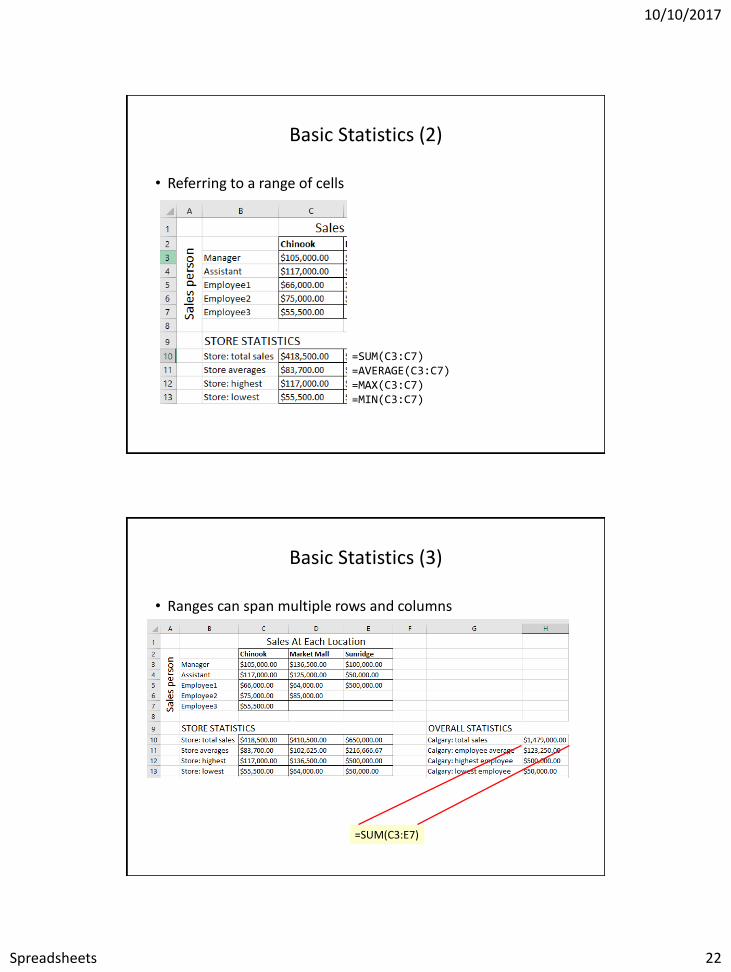
Excel String Functions
• Functions that act on strings
• Converting or changing alphabetic text– Change text from one form to another
– lower(), upper(), proper()
• Processing text– Remove spaces
– Trim()
• Connecting text: – connecting a string or a part of that string with another string e.g. title
with surname or first name
– concatenate()
Excel String Functions (2)
• Extract selected portions of text: – A specific number of characters from some position are to be extracted
from a string e.g., area code or country code from a phone number
– left(), right(), mid()
• Searching text (useful support function when extracting text) – Finds the starting position of one string within another string
– find()

10/10/2017
Spreadsheets 27
Functions That Convert Text
lower()
• Converts non-lower case alphabetic characters to lower case• https://support.office.com/en-US/article/LOWER-function-3F21DF02-A80C-44B2-AFAF-81358F9FDEB4
upper()
• Converts non-upper case alphabetic characters to upper case• https://support.office.com/en-US/article/UPPER-function-C11F29B3-D1A3-4537-8DF6-04D0049963D6
proper()
• For alphabetic text it converts the letters to ‘proper’ format:
– All letters are lower case except for the first letter of each word (which is capitalized)
– Example word separators: space, dash, underscore• https://support.office.com/en-US/article/PROPER-function-52A5A283-E8B2-49BE-8506-B2887B889F94
Functions That Convert Text (2)
• Example spreadsheet: “9_converting_text”

10/10/2017
Spreadsheets 28
Functions For Extracting And Connecting Text
trim():
– Removes leading or trailing spaces (multiple spaces within text are trimmed to a single space)
– Format: trim(<string>)
– Examples:
• = Trim(" james ")
• = Trim(" a b ")– https://support.office.com/en-US/article/TRIM-function-410388FA-C5DF-49C6-B16C-9E5630B479F9
concatenate():
– Connects two or more strings
– Format: concatenate(string1, string2…)
• A string can be fixed e.g., concatenate(“wa”,”sup”) or the address of a cell e.g., concatenate(A1,”!”)
– https://support.office.com/en-US/article/CONCATENATE-function-8F8AE884-2CA8-4F7A-B093-75D702BEA31D
Functions For Extracting And Connecting Text (2)
left():– Extracts the specified number of characters from the left side of the
specified string.
– Format: left(<string>, <length>)• String: the source string to extra characters from
• Length: the number of characters to extract– https://support.office.com/en-US/article/Left-Function-D5897BF6-91F5-4BF8-853A-B63D7DE09681
– Examples:
=left("Foo bar",2)
=left("Foo bar",0)
=LEFT("Foo",10)

10/10/2017
Spreadsheets 29
Functions For Extracting And Connecting Text (3)
right():– Extracts the specified number of characters from the right side of the
string
– Format: right(<string>, <length>)– https://support.office.com/en-US/article/Right-Function-C02A18A8-B224-437E-AABA-1B785C6C61BF
– Examples:
=RIGHT("Foo!bar",2)
=RIGHT("Foo",10)
Functions For Extracting And Connecting Text (4)
mid():
– Starting at the specified position, the function extracts the specified number of characters from the string
– Format: mid(<string>, <start>, <length>)
• String: the source string to extra characters from
• Start: the position in the string in which extraction should begin
• Length: the length of the sub-string to extract (sub-string begins at the position specified with the ‘start’ argument)
– https://support.office.com/en-US/article/Mid-Function-427E6895-822C-44EE-B34A-564A28F2532C
– Examples:
=MID("not too hot",2,4)
=MID("not too hot",8,55)
=MID("not too hot",0,5)
=MID("not too hot",7,0)
10/10/2017
Spreadsheets 30
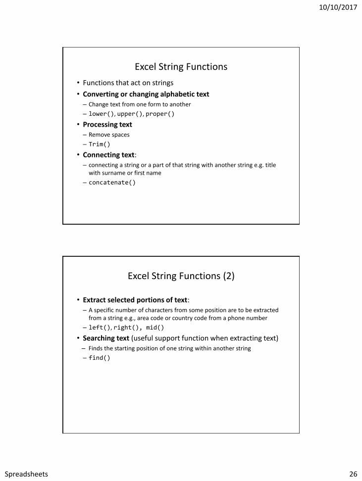
Using One Function’s Return Value As Input For Another Function (Nesting Functions)
• Breaking down the process into parts1. Call a function and that function returns a
value
2. Use the return value of that function as part of the input of another function
sum(2,4)
Returns 6
=average( ,6,12)
Actual formulation of the function=average(sum(2,4),6,12)
Functions For Extracting And Connecting Text (5)
find():– Finds the starting position of one string within another string
– Format:
• find(<find text>, <within text>, [<start position>])
– Find text: search for the first occurrence of the find text within the within text
– Within text: the string on which the search is performed
– Start number (optional): the position of the ‘within text’ that you want the search to being
– https://support.office.com/en-US/article/FIND-function-06213F91-B5BE-4544-8B0B-2FD5A775436F
– Examples:
• =FIND("me", "james")
• =FIND("la","fa-la-la-la-la")
• =FIND("la","fa-la-la-la-la",6)
• =FIND("x","XYZ")

10/10/2017
Spreadsheets 31
Extracting And Connection Text: More Examples
• Example spreadsheet: “10_extracting_connecting_text”
Combinations: Find(), Mid()
• The return value of one function can be used as the argument of another function.
• Consider this example– Cell A10 contains the string “Apt #709, 944 Dallas Dr. NW”
– You wish to extract the apartment number as well the preceding number sign #ddd into a substring
– Assume that apartment numbers are always preceded by the number sign #
– Also you assume that apartment numbers are three digits in length
– You cannot make assumptions about the information that precedes the number sign (zero to ‘infinity’)
– Find() can be use to determine the start location of the apartment in the string
• FIND("#",A10)
– The start position of the apartment information can be used as one of the arguments for an extraction function

10/10/2017
Spreadsheets 32
Combinations: Find(), Mid(): 2
– =MID(A10, ,4)
– But you can’t always assume that the apartment information begins at position five.
• “Apt #709, 944 Dallas Dr. NW”
• “#123, 4944 Dalton Dr NW”
• So the return value from find() must be used to first determine the location of the apartment information.
• Next this information is used as one of the arguments for the mid(), string extraction function.
• All together: “=MID(A10,FIND("#",A10),4)”
5
=MID(A10, ,4)
FIND("#",A10)
5
Why Bother?
• When would you ever use Excel functions this way?
• Sometimes the data has already been entered into the sheet – Data may combine fields or include extraneous information:
– 403-123-4567 (postal code and phone number combined, dash)
– (403)111-2222 (as above but adds additional brackets)
1. Labor saving– Retyping a large dataset (after removing extraneous information) may be
time consuming
– Solve the problem once and then reuse (copy and paste) the trimming formula wherever else it is needed

10/10/2017
Spreadsheets 33
Why Bother? (2)
2. Different views of the same data may be needed (from an earlier example sheet): 10_extracting_connecting_text
– In Canada the proper greeting will be “Prof. Tam” (Title, Last name)
=CONCATENATE(A2,C2)
– In other countries the proper greeting will be “Prof. James” (Title, First name)
=CONCATENATE(A2,B2)
Why Bother? (3)
3. It may useful to be familiar with these functions for the future!
• Job interviews, the exams, the bonus feature of the assignment ;)

10/10/2017
Spreadsheets 34
Lecture Exercise #1: String Functions
Lecture Exercise #1: String Functions

10/10/2017
Spreadsheets 35
Lecture Exercise #2: Tracing String Functions
Lecture Exercise #3: String Functions (You Do)

10/10/2017
Spreadsheets 36
Date And Time Functions
• Example spreadsheet:“11_date_time”
• today()– Displays the current date (month/day/year) e.g., 07/15/2015
• now()– Displays the current date (as above) and time (hour/minute with a 24
hour clock) e.g., 18:42
• Both: determine the time/date based on the settings of the computer on which the worksheet is run.– Updates occur when the files is opened or when the spreadsheet
recalculates new values.
‘If-Else’ (Branching)
• Function returns one value if a condition has been met. (True)– “If condition met do an action”
• Function can return another value if the condition hasn’t been met. (False)– “Else if the condition not met do another action”
• Boolean (logic): either true or false that the condition was met
Grade point >= 1.0
“Passed”
True
“Failed”
False

10/10/2017
Spreadsheets 37
Applying Branches: Grade Example
• In column ‘E’ the sheet will display “GO!” if net income is 100 (millions of $) or greater “Don’t waster your $” otherwise.– Example spreadsheet: 12_if_invest_or_not
=IF (B2>=100, "GO!", "Don’t’ waste your $")
Condition Action: condition true
Action: condition false - “else case”
Format: IF-Else
• Format:=if (<condition to check>,
<return value: condition true>,
[<return value: condition false>])
• Example:=IF (B2>=100,"GO!","Don’t’ waste your $")
• Note: the return value is not limited only to text– Some example return values IF-Else: text, numeric, a cell reference e.g. =IF(A1>1,A1,A2)
• https://support.office.com/en-US/article/IF-function-69aed7c9-4e8a-4755-a9bc-aa8bbff73be2?CorrelationId=6aeb3056-a94b-47ac-af6e-90dff250a029

10/10/2017
Spreadsheets 38
Comparators
Math Excel Meaning
< < Less than
> > Greater than
= = Equal to
≤ <= Less than, equal to
≥ >= Greater than, equal to
≠ <> Not equal to
If: Specifying Only The True Case (Poor Approach)
• If only a return value for the true case has been specified:– When the condition has not been met (false that the condition has been
met) i.e., “Has the student passed the course?”…literally the text “FALSE” will be displayed.
– No spreadsheet example has been provided because this implementation is incorrect
• To see the result you can edit the previous sheet and just delete the false case “Don’t waste your…” message (False return case in ‘Column C’ data).
=IF(B4>=100,"GO!")

10/10/2017
Spreadsheets 39
• Consequently: – Even if a specific return value is desired only for the ‘if condition case’
(true that the condition has been met)
– Something, even an empty message, should be specified for the ‘else return case’ (false that the condition has been met).
• Previous example: amended– Example spreadsheet: 13_if_invest_only
If: Specifying Only The True Case (Better Approach)
=IF(B4>=100,"GO!","")
Nested Conditions
• Conditions that are dependent upon or are affected by previous conditions.
• ‘Nest conditions’ refers to conditions that are ‘inside of other conditions’
• Example (assume that the respondent previously indicated that his or her birthplace was an Alberta city)
• Select the AB city in which you were born
1. Airdrie
2. Calgary
3. Edmonton
…
– Selecting Airdrie excludes the possibility of selecting Calgary
– Cities listed later are ‘nested’ in earlier selections because they won’t be checked if an earlier selection is true)

10/10/2017
Spreadsheets 40
Nested Conditions (2)
• Applies when different conditions must be checked but at most only one applies (exactly 0 or 1 conditions can be true)
• Example:– Display “Terrific” if net income 100 or greater
– Display “Excellent” if net income is 50 or greater but less than 100
– Display “Adequate” if net income is 25 or greater but less than 50
– Display “Poor” if net income is 10 or greater but less than 25
– Display “Terrible” if net income is 0 or greater but less than 10
– Otherwise “Error” will be displayed
• Example spreadsheet: 14_nested_if_investments
Previous Example: Specifying Conditions
income>=100? “Terrific”True
“Error”
False
income>=50? “Excellent”True
False
income>=25? “Adequate”True
False
income>=10? “Poor”True
False
Nesting• Later conditions are
described as being ‘nested’ within earlier conditions
• The Net income cases for 50+, 25+, 10+, 0+ are described as being ‘nested’ within the 100+ case (only checked if the previous case proves to be false)
income>=0?
False
“Terrible”True

10/10/2017
Spreadsheets 41
Nested “If’s”
• Format:=IF(<condition to check>,<return: true>,[<return: condition false>])
• Example:=IF(B2>=100,"Terrific", )
if (<condition to check>, <return: true>, <return: false>)Another if-check
IF(B2>=50,"Excellent","")
Previous Example: Initial Cases
• If income>=100 “Terrific”, if 50<=income<100, “Excellent”
TRUE>=100
FALSE>=100
100<TRUE>=50
This 2nd expression is implied by the IF(don’t literally type it in expressions after
the 1st for nested IFs)

10/10/2017
Spreadsheets 42
Previous Example: Nested Solution=IF(B2>=100, "Terrific",
IF(B2>=50,"Excellent",IF(B2>=25,"Adequate",
IF(B2>=10, "Poor",IF(B2>=0, "Terrible", "Error")))))
=IF(B2>=100,"Terrific",IF(B2>=50,"Excellent",IF(B2>=25,"Adequate",IF(B2>=10,"Poor",IF(B2>=0,"Terrible","Error")))))
F
F
FF
F
Nesting Ifs: Order Is Important
• (Checking numeric ranges): Specify the largest range first– Correct
• IF (A1 >= 100, "Terrific", IF(A1 >=50,"Excellent", ""))
• A1 contains 175 and “Excellent” appears (right)
– Incorrect
• IF (A1 >= 50, "Excellent", IF(A1 >= 100,"Terrific", ""))
• A1 contains 175 and “Excellent” appears (wrong)

10/10/2017
Spreadsheets 43
Lookup Functions
• Can (should/must) be employed instead of many nested IF’s.– Easier to enter, update, understand.
• Requirements of previous example:0 <= Income < 10 : Terrible
10 <= Income < 25 : Poor
25 <= Income < 50 : Adequate
50 <= Income < 100 : Excellent
Income >= 100 : Terrific
• Previous solution:=IF(B2>=100,"Terrific",IF(B2>=50,"Excellent",IF(B2>=25,"Adequate",IF(B2>=10,"Poor",IF(B2>=0,"Terrible","Error")))))
Lookup Functions
• The lookup functions that will be covered this semester will be used in conjunction with a lookup table or tables.– Nested IFs can and should also use a lookup table
• Two lookup functions covered include:– LOOKUP() (If there is time)
– VLOOKUP()
– (Not that the ‘IF’ is not classified as a lookup function!)
• For a complete list of lookup functions in Excel:– https://support.office.com/en-US/article/Lookup-and-reference-functions-reference-8aa21a3a-b56a-4055-8257-3ec89df2b23e

10/10/2017
Spreadsheets 44
LOOKUP: If There’s Time
• https://support.office.com/en-US/article/LOOKUP-function-446D94AF-663B-451D-8251-369D5E3864CB
• Typical use:– Looking up a value from one column (“a vector”)
– Return a value from another column (“a vector”)
– (According to Microsoft): if you want to look up values from multiple columns (“an array”) then the VLOOKUP function should be used instead of LOOKUP.
=CONCATENATE(F1, LOOKUP(B2,E4:E5,F4:F5))LOOKUP(B2,E4:E5,F4:F5)
LOOKUP (2) : If There’s Time
• Format:LOOKUP(<Lookup value>,
<Lookup column (vector) Start : End>,
<result column (vector) Start : End>)

10/10/2017
Spreadsheets 45
LOOKUP (3) : If There’s Time
• Example spreadsheet: 15_lookup
• Row 2 data
=LOOKUP(B2, D11:D15, E11:E15)
Cell: Contains value to find in table e.g., net income
Lookup column:Start : End cell coordinates
Result column:Start : EndCell coordinates
LOOKUP (4) : If There’s Time
=LOOKUP(B3,D11:D15,E11:E15)
Min income Comment
0 Terrible
10 Poor
25 Adequate
50 Excellent
100 Terrific
D E
11
12
13
14
15
>50?
>50?
>50?
>50?
>50?..Yes! Backup and use this value Return “Excellent”
A lookup table used in conjunction with LOOKUP must be sorted in ascending order

10/10/2017
Spreadsheets 46
LOOKUP: Multi-Column Lookup Table (If There’s Time)
• Name of example spreadsheet: 16_lookup_multiple_columns
Lookup table
LOOKUP function
VLOOKUP
• A more complicated (but more powerful) version of a lookup function.
• https://support.office.com/en-US/article/VLOOKUP-function-0BBC8083-26FE-4963-8AB8-93A18AD188A1
• Format:VLOOKUP(<Lookup value>,
<Lookup table Start : End>,
<Lookup table Column specifying the return value>,
[<Exact match required?>])
• Example:=VLOOKUP(B2, D11:E15, 2)
Cell: Contains value to find in table e.g., a grade point
Lookup table:Start : End cell coordinates
Lookup table:Column value to return (1 = first col. ‘D’, 2 = second col. ‘E’)

10/10/2017
Spreadsheets 47
VLOOKUP: Previous Example
Min income Comment
0 Terrible
10 Poor
25 Adequate
50 Excellent
100 Terrific
=VLOOKUP(B2,D11:E15,2)
Example spreadsheet: 17_vlookup
D E
11
12
13
14
15
Col 1 Col 2
VLOOKUP: Multi-Column Lookup Table
• Name of example spreadsheet: 18_vlookup_multiple_columns
Lookup
function
Lookup tableCol 1 Col 2 Col 3

10/10/2017
Spreadsheets 48
VLOOKUP: Optional Value = TRUE (True = Approximate matches allowed)
• VLOOKUP example:=VLOOKUP(B3,C11:E15,3,TRUE))
• TRUE (works like LOOKUP so the lookup table values must be sorted)– Look for an approximate match.
– If an exact match is not found, the next largest value that is less than lookup value is returned.
– If T/F value is omitted then the function assumes a ‘TRUE’ value.Min income Comment
0 Terrible
10 Poor
25 Adequate
50 Excellent
100 Terrific
Income = 50
>50?
>50?
>50?
>50?
>50?..No!
Backup and use this value Return “Excellent”
VLOOKUP: Optional Value = FALSE (False = Approximate matches Not allowed, exact matches
required)
• VLOOKUP example:=VLOOKUP(B2,C11:E15,3,FALSE))
• FALSE:– Looks only for an exact match
– If a match is found then the value at the specified location is returned.
– Else if no match is found the an error message is displayed.
– Table values do not have to be sorted when the False optional argument is passed to the VLOOKUP function.

10/10/2017
Spreadsheets 49
VLOOKUP: Optional Value = TRUE/FALSE
• TRUE– Use when looking a value in a range of values (must be in ascending
order) E.g. grades, tax brackets
• FALSE:– Use when there is an exact value to lookup (order is not important) e.g.,
SIN numbers, product ID number
Income range Min for range Tax rate
0 - $20,000 0 0%
> $20,000 20,000 10%
Product number Name Price
B00KAI3KW2 Xbox One $449
B00BGA9WK2 Playstation 4 $449
Example: Sensible Use Of False/VLOOKUP
• Name of example spreadsheet: 19_vlookup_false
• Reminder:– Use when exact matches are required
– Lookup table does not have to be sorted
Lookup table
Lookup function

10/10/2017
Spreadsheets 50
Looking Values: If Function Vs. Lookup Functions
• Multiple IFs: – Can be used if there are only a handful of conditions to check (rule of
thumb: 2 – 3 max e.g., 2 conditions)
– Complex and error prone for anything else (e.g. 5 conditions)
• Lookup functions– Steeper learning curve (but a “one-time investment”)
– Once learned the formulas are simpler (no nesting) and less error prone
=IF(B2>=100,"Terrific",IF(B2>=50,"Excellent",IF(B2>=25,"Adequate",IF(B2>=10,"Poor",IF(B2>=0,"Terrible","Error")))))
=IF(D2>=3, "Honors",IF(D2>=0, "Pass","Fail"))
=VLOOKUP(B2,D11:E15,2) Min income Comment
0 Terrible
10 Poor
… …
When To Use The IF-Function
• When multiple conditions must be checked– Combined with the logical operators (typically AND, OR - although NOT
may also be used)

10/10/2017
Spreadsheets 51
Logical Operations In Excel
• The basic logical operations: AND, OR, NOT can be invoked as functions in Excel– All function inputs can only be a True or False value.
– Function inputs can be:
• Boolean constant e.g. NOT(True), AND(True,False)
• Boolean expression e.g. NOT(C2>0), OR(A1>0,A2>0)
• A cell that contains a Boolean value e.g. NOT(C2), AND (A1,A2)
• Format:AND(<True or False>,<True or False>...)
OR(<True or False>,<True or False>...)
NOT (<True or False>)
• Examples (spreadsheet name: 20_logicAND(C1>=45,D1="John Smith") # Requires all
OR(C1>=0,D2>=0) # Requires at least one
NOT(AA12) # Reverses the logic
Logic And IF’s: Example
• The honor roll for each semester requires that grade point is 3.7 or greater and a full load of at least 5 courses must be taken.
• AND Example: Dean’s list– Signify when a student has made the Dean’s list requirements with an
“H”, blank cell otherwise.
• Example spreadsheet: 21_if_logic
=IF(AND(B4>=3.7,C4>=5),"H","")

10/10/2017
Spreadsheets 52
Logic And IF’s: Example (2)
• OR Example: Hiring if at least one requirement met (work experience of 5+ years, grade requirement of 3.7 or higher)– (Same spreadsheet as previous example)
=IF(OR(E12>=5,G16>=3.7),"1+ requirement met","")
E12
G16
Lecture Exercise #4: Branching (And Other) Functions

10/10/2017
Spreadsheets 53
Conditional Counting Functions
• Increases a tally count if one or conditions have been met
• COUNTIF(): count if a particular condition has been met
• COUNTIFS(): count if all conditions have been met
Counting Functions Based On Conditions: Countif()
• Counts the number of cells that meets a particular requirement– https://support.office.com/en-US/article/COUNTIF-function-E0DE10C6-F885-4E71-ABB4-1F464816DF34
=COUNTIF(C13:C16,">0")

10/10/2017
Spreadsheets 54
Counting Functions Based On Conditions: Countif(), 2
=COUNTIF(C13:C16,"B")
Counting Functions Based On Conditions: Countifs(), 3
• Can be used when multiple requirements must be met:– Counts the number of cells that meets all in a series of multiple
requirements– https://support.office.com/en-US/article/COUNTIFS-function-DDA3DC6E-F74E-4AEE-88BC-
AA8C2A866842
• Format:=countifs(
<range 1>, <criteria 1>,
… <optional additional range>, [<optional additional
criteria>])
• Example spreadsheet: 22_conditional_counting_formulas– =countifs(A1:A10,"A", B2:B7, ">=100")

10/10/2017
Spreadsheets 55
Counting Functions: Countifs(), 4
Specify: count number of employees that met the quota for both months
Col C Col D
14
151617
18
19
Conditional Formatting
• A very practical example of how conditional branching “if’s” can be applied.
• Use of conditional formatting will be covered in tutorial.

10/10/2017
Spreadsheets 56
Methods Of Referring To Cells
• Absolute: – The formula won't change if you copy/cut and paste the formula or if the
spreadsheet changes in size
• Relative– The formula changes depending how far that the formula is moved or
how much the spreadsheet is changed in size.
Absolute Reference
• When a reference to an cell or range of cells doesn’t change when the contents of a cell or cells is copied or the sheet changes in size.
Original formula (B12)
=$B$1-B10
Copied (C12)
=$B$1-C10
Assumption
Row 10 sums row 4 – 9.

10/10/2017
Spreadsheets 57
Absolute Reference (2)
Original formula (B12)
=$B$1-B10
Copied (C12)
=$B$1-C10
Absolute
referenceAbsolute
reference
Absolute reference because the same (absolute) reference to cell B1 is
made when the formula is copied.
Absolute Reference (3)
• Typically it’s used in conjunction with constants (data that won’t change).
Original formula (B12)
=$B$1-B10
Copied (C12)
=$B$1-C10
References to B1 are
absolute because
income doesn’t
change

10/10/2017
Spreadsheets 58
Relative Reference
• A reference to a cell or group of cells that may change if the cell/cells are copied or the sheet changes in size.
Original formula (B12)
=$B$1-B10
Copied (C12)
=$B$1-C10
Relative Reference (2)
Original formula (B12)
=$B$1-B10
Copied (C12)
=$B$1-C10
Reminder:
• Total expenses (row 10) is
a calculated value. It sums
rows 4 – 9.
Relative
reference
Relative
reference
Relative reference because the copied formula will change relative to
how far it’s copied.

10/10/2017
Spreadsheets 59
Relative Reference (3)
• Typically it’s used with variable data (that may change over time or in different parts of the sheet).
Original formula (B12)
=$B$1-B10
Copied (C12)
=$B$1-C10
Total expenses may
change from month-
to-month so
references will likely
be relative.
Cell References: Important Details
• Format: specify absolute cell references with a dollar sign ‘$’ immediately in front of the row or column value.[<dollar sign for column>]<column> [<dollar sign for row>]<row>
• Examples:– Relative column, relative row: A1
– Relative column absolute row: A$1
– Absolute column, relative row: $A1
– Absolute column, absolute row: $A$1

10/10/2017
Spreadsheets 60
Absolute, Relative And Mixed References: Examples1
Example Reference type Copied result
$A$1 •Absolute column
•Absolute row
$A$1
A$1 •Relative column
•Absolute row
C$1
$A1 •Absolute column
•Relative row
$A3
A1 •Relative column
•Relative row
C3
1 Examples from the Excel 2003 Help System
• Example spreadsheet: 23_absolute_relative
Absolute, Relative References: Example
Original formulas (result)
=$C$4 (4)=B$3 (1)=$A2 (2)=A2 (2)
COLUMN F
ROWS
11
12
13
14
To E7
To G8
To D14
To G16

10/10/2017
Spreadsheets 61
Absolute/Relative Applied To A Previous Example
• Which part of the formula should be:– Absolute?
– Relative?
– Why?
= (B3*G2)+(C3*G3)
= (B4*G3)+(C4*G4)
Lecture Exercise #5: Absolute, Relative Addressing (If There Is Time)
10/10/2017
Spreadsheets 62
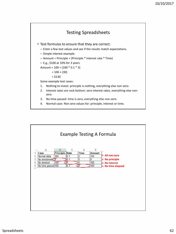
Testing Spreadsheets
• Test formulas to ensure that they are correct.– Enter a few test values and see if the results match expectations.
– Simple interest example:
– Amount = Principle + (Principle * Interest rate * Time)
– E.g., $100 at 10% for 3 years
Amount = 100 + (100 * 0.1 * 3)
= 100 + (30)
= $130
Some example test cases:
1. Nothing to invest: principle is nothing, everything else non-zero.
2. Interest rates are rock bottom: zero interest rates, everything else non-zero
3. No time passed: time is zero, everything else non-zero.
4. Normal case: Non zero values for: principle, interest or time.
Example Testing A Formula
<- All non-zero
<- No principle
<- No interest<- No time elapsed

10/10/2017
Spreadsheets 63
Testing Ranges
• The following are the minimum test cases
• Provide test values for each range– In this example try grade points of 0, 1, 2, 3, 4
• Also for at least one of the ranges test the boundaries (just above and below)– Example: testing the boundary for 1 / “Pass”
• Slightly below a boundary value e.g., 0.9 should return “Fail”
• Slightly above a boundary value e.g., 1.1 should return “Pass”
• Total test cases for this example: 7 tests
Min. GPA Comment
0 Fail
1 Pass
2 Adequate
3 Excellent
4 Perfect
Example: Good Design And Testing
• Previous grading example: the following will likely be data (cannot be calculated from other values in the sheet)
• Values that will be determined by the data– “Term grade point” (calculated), “Comments” (lookup)
10/10/2017
Spreadsheets 64
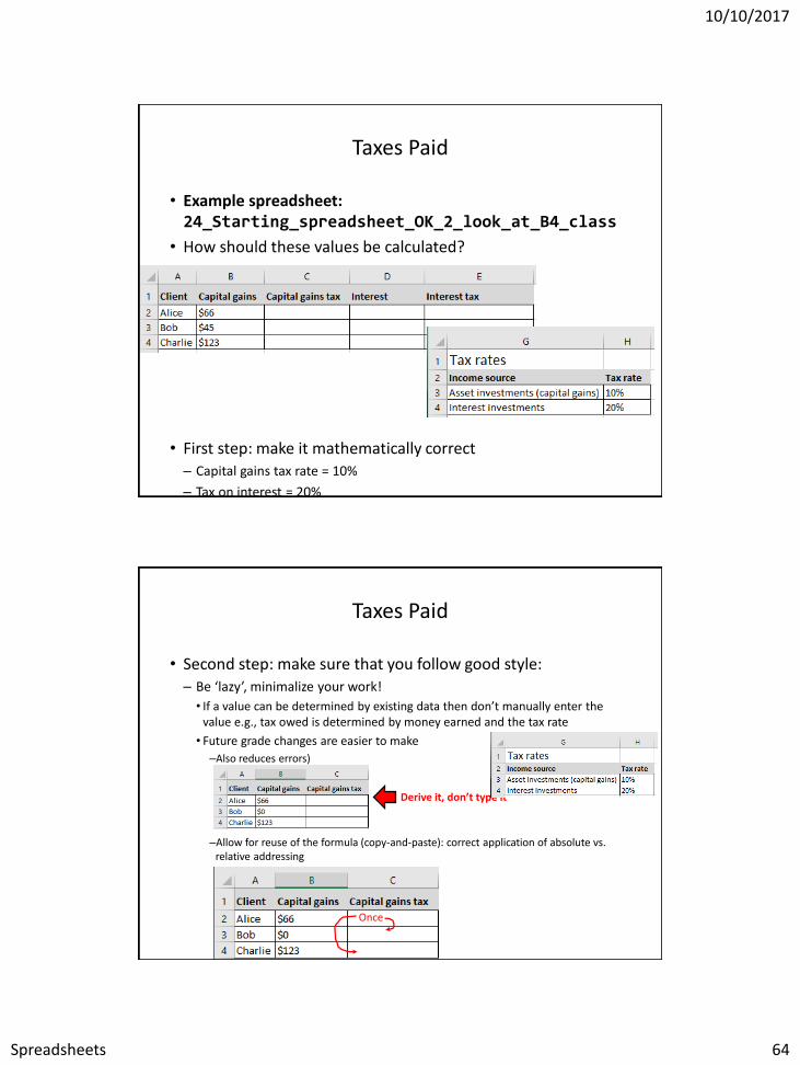
Taxes Paid
• Example spreadsheet: 24_Starting_spreadsheet_OK_2_look_at_B4_class
• How should these values be calculated?
• First step: make it mathematically correct– Capital gains tax rate = 10%
– Tax on interest = 20%
Taxes Paid
• Second step: make sure that you follow good style:– Be ‘lazy’, minimalize your work!
• If a value can be determined by existing data then don’t manually enter the value e.g., tax owed is determined by money earned and the tax rate
• Future grade changes are easier to make
–Also reduces errors)
–Allow for reuse of the formula (copy-and-paste): correct application of absolute vs. relative addressing
Once
Derive it, don’t type it

10/10/2017
Spreadsheets 65
Tax Owed
• Example spreadsheet: 25_Starting_spreadsheet_OK_2_look_at_B4_CLASS
• How should this value be derived?– Use the cutoff values in the table below.
– Remember it must be correct AND it should follow good style conventions.
Absolute, Relative: Completed Examples
• Names of the spreadsheets with solutions (don’t look at contents before we go over the concepts in lecture) – 24_DON'T_look_at_B4_class
– 25_DONT_LOOK_B4_CLASS

10/10/2017
Spreadsheets 66
Graphical Design Principles
• Using color
• Fonts and font effects
• C.R.A.P.
Color: Properly Used
• When used sparingly color can draw attention to important information.
• This is an especially valuable tool when there is a large amount of information.– The information may be “all there” but don’t make it any harder than it
has to be for the viewer to find it.

10/10/2017
Spreadsheets 67
Color Misused
• The overuse of color: – Reduces it’s ability to make information stand out.
– Makes it harder to understand what information is mapped to a particular color e.g. using different colors to represent faculty and grades
Rule Of Thumb For Color: Make It Subtle
• We have all seen the use of ‘loud’ and clashing colors that can make text very hard to read.
IngredientsSugar, lactose, fructose, corn syrup, glucose…lots of carbohydrates
JT: I’ve actually seen green-red color combinations on listings of food ingredients

10/10/2017
Spreadsheets 68
Rule Of Thumb For Color: Subtle But Not Near-Invisible
• The “flip side”, lack of contrast between foreground can also be problematic.
IngredientsSugar, lactose, fructose, corn syrup, glucose…lots of carbohydrates
Rule Of Thumb For Color
• Balance the use of color between noticeability and subtlety– Make it as subtle as possible while still conveying the necessary
information using color

10/10/2017
Spreadsheets 69
Additional Issues Associated With Color
• Color blindness affects a portion of the population:– The majority of people who are color blind are red-green color blind so
using only these colors to represent information should be avoided e.g. traffic lights
• Field size– The larger the area to be color coded, the more easily that colors can be
distinguished.
Larger areas: colors can be more subtle
Smaller areas: colors may have to employ greater contrast
Additional Issues Associated With Color (2)
– When objects are small (text or small graphics) and color is used to distinguish information use highly saturated colors.
This is
important
information!
This is
important
information!

10/10/2017
Spreadsheets 70
Fonts And Font Effects
• Example fonts:– Ariel
– Calibri
– Helvetica
– Times New Roman
• Font effects:– Italics
– Bold
– Underline
– Normal
• Font sizes
Fonts And Font Effects (2)
• As a rule of thumb use no more than 3 sizes and font effects / font sizes in a particular document.– Similar to color, their overuse reduces their effectiveness and makes it
harder to interpret meaning.
• Also if you don’t know much about fonts just stick to the common or default ones provided (Arial, Calibri, Helvetica, Times New Roman)
– If you’re not sure if a font is a good one for a particular situation then it probably isn’t:
• Extreme example “Wing dings”: wing dings
• But the use of “extreme fonts” are the only pitfall: printing problems, web browser issues, operating system font-issues.
• Example (from http://docs.oracle.com...
/cd/E19728-01/820-2550/printing_pdffonts.html)

10/10/2017
Spreadsheets 71
C.R.A.P.1
• Simple design principles that can be applied in a variety of situations
• Contrast
• Repetition
• Alignment
• Proximity
1 From “The non-designers type book” by Robin Williams (Peach Pit express)
Contrast & Repetition
• Contrast:– Make different things look significantly different
• Repetition (Consistency): – Repeat conventions (e.g. fonts, font effects, alignment, colors used)
throughout the interface to tie elements together e.g. headings are all formatted consistently

10/10/2017
Spreadsheets 72
Example: No Contrast
Example: Weak Contrast

10/10/2017
Spreadsheets 73
Example: Headings Stand Out
• Good contrast:– If contrast is not (or weakly) employed for a small set of data it may not
be a large issue.
– But for larger data sets (“real data”) it may make it more work than is necessary.
• Repetition:– Same fonts, font sizes and font effects used in the headings vs. the data.
– Makes it easier to see and understand the structure
Repetition (Previous Example)
• Headings vs. data/body, consistency with:
– Font effect (bold)
– Font size
– Font type
– Alignment

10/10/2017
Spreadsheets 74
Alignment
• It can be used to structure a document (represents hierarchical relationships).
Alignment And Repetition
• Consistent alignment (left or right and not center) can be used to represent relationships.– All the data in a column are consistently aligned to signify they belong a
group
• Example: movie credits
The Kung Fu master
Arch villain
Kung Fu student #1
Kung Fu student #2
Thug #1
Thug #2
Damsel in distress
James “The Bullet” Tam
James (Evil dude) Tam
Eager Tam1
Eager Tam2
Cannon-fodder Tam #1
Cannon-fodder Tam #2
Jamie Tametta

10/10/2017
Spreadsheets 75
Center Alignment
Centre Alignment (2)
• Don’t use it for hierarchical documents because it removes or hides the organization.– In a document that contains structure center alignment can look
unorganized (the center alignment appears as no alignment, disorganized)
• At most: sparing use can be used to provide contrast e.g., slide titles vs. content.
• Because it removes a common method for structuring a document it can make reading text more difficult.
• At most use it as an exceptional case to make an item stand out.

10/10/2017
Spreadsheets 76
Center Alignment
• Again: while sparing use of center alignment can be used to provide contrast it should NEVER be used as the default in documents such as spreadsheets.
Example: When Center Alignment Is Probably Okay

10/10/2017
Spreadsheets 77
Proximity
• Related items are in close proximity
• Unrelated items are separated
After This Section You Should Now Know
• The benefit of electronic over paper spreadsheets
• Spreadsheets 101: The basic layout and components of a spreadsheet
• What is a worksheet– When to use multiple spreadsheets vs. multiple worksheets
– How to reference data in other spreadsheets or worksheets (cross references)
• How Excel groups functions according to tabs on the ribbon– What are the most commonly used tabs and what some of the functions
available on those tabs
• Entering data: manually and via autofill
• How to freeze data

10/10/2017
Spreadsheets 78
After This Section You Should Now Know (2)
• Tags– How to do tag a spreadsheet
– What is the benefit of using tags
• Common mathematical operators and the order of operation
• What is the difference between constants (data) and calculations (formulas)– How is a formula differentiated from data
• The three rules of thumb for designing spreadsheets1. Don’t make something data if it can be derived
2. Label everything
3. Don’t duplicate data
After This Section You Should Now Know (3)
• Lookup tables– How to create a use a lookup table
• Formulas:– Directly entering custom formulas
– Using built-in pre-created formulas
– What is the order of operation for common operators
• How to format cells using the “format cell” option– What is the effect of different numeric formatting options
• How to use basic statistical formulas: sum(), average(), min(), max()
• How to use counting functions: count(), counta(), countblank, countif(), countifs()

10/10/2017
Spreadsheets 79
After This Section You Should Now Know (4)
• How to use string functions: lower(), upper, proper(), trim(), concatenate(), find(), left(), right(), mid()
• How to use the today(), now() functions
• How to use ‘if-else’ for branches that return different values– The different ways of expressing logical comparators
– How to write or evaluate nested ‘if’s’
• Logical operations in Excel: AND, OR, NOT– How to write or evaluate logical operations
– How to apply the logical operations in conjunction with the ‘if-else’
• How to use the LOOKUP(), VLOOKUP function
After This Section You Should Now Know (5)
• How to come up with set of reasonable test cases for a spreadsheet– Formulas and ranges
• What is the difference between an absolute vs. relative cell reference and when to use each one

10/10/2017
Spreadsheets 80
After This Section You Should Now Know, Design (6)
• Rules for using and not misusing color as well issues associated with color: color blindness and field size
• Rules of thumb for using fonts and font effects
• C.R.A.P.– What does each part mean
– How it can be used for effective graphic design
Copyright Notification
• “Unless otherwise indicated, all images in this presentation are used with permission from Microsoft.”
• Images of spreadsheets (save VisiCalc) are curtesy of James Tam