CERN-TH-2017-186

NORDITA-2017-093

TAUP-3023/17

Spontaneous CP breaking in QCD and the axionpotential: an effective Lagrangian approach

Paolo Di Vecchiaa,b, Giancarlo Rossic,d, Gabriele Venezianoe,f ,Shimon Yankielowiczg

a The Niels Bohr Institute, Blegdamsvej 17, DK-2100 Copenhagen Ø, Denmarkb Nordita, KTH Royal Institute of Technology and Stockholm University,

Roslagstullsbacken 23, SE-10691 Stockholm, Swedenc Dipartimento di Fisica, Universita di Roma “Tor Vergata” and INFN Sezione Roma 2,

Via della Ricerca Scientifica - 00133 Roma, Italyd Centro Fermi - Museo Storico della Fisica e Centro Studi e Ricerche “E. Fermi”

Piazza del Viminale 1 - 00184 Roma, Italye College de France, 11 place M. Berthelot, 75005 Paris, FrancefTheory Division, CERN, CH-1211 Geneva 23, Switzerland

g School of Physics and Astronomy, Tel-Aviv University, Ramat-Aviv 69978 Israel

Abstract

Using the well-known low-energy effective Lagrangian of QCD –valid for small (non-

vanishing) quark masses and a large number of colors– we study in detail the regions of

parameter space where CP is spontaneously broken/unbroken for a vacuum angle θ =π. In the CP broken region there are first order phase transitions as one crosses θ =π, while on the (hyper)surface separating the two regions, there are second order phase

transitions signalled by the vanishing of the mass of a pseudo Nambu-Goldstone boson

and by a divergent QCD topological susceptibility. The second order point sits at the

end of a first order line associated with the CP spontaneous breaking, in the appropriate

complex parameter plane. When the effective Lagrangian is extended by the inclusion of an

axion these features of QCD imply that standard calculations of the axion potential have

to be revised if the QCD parameters fall in the above mentioned CP broken region, in

spite of the fact that the axion solves the strong-CP problem. These last results could

be of interest for axionic dark matter calculations if the topological susceptibility of pure

Yang-Mills theory falls off sufficiently fast when temperature is increased towards the QCD

deconfining transition.

arX

iv:1

709.

0073

1v3

[he

p-th

] 2

2 D

ec 2

017

1 Introduction

Already in the early seventies Dashen recognized [1] that phases in the quark mass matrixcould spontaneously break CP and the possibility that such a phenomenon could explainthe observed CP violation in kaon physics was explored [2]. It turned out that theseviolations were too large to explain the experiments with K mesons and would give amuch too high value for the electric dipole moment of the neutron and for the η → 2πdecay amplitude [3]. At about the same time Weinberg pointed out [4] that possible CPviolating phases can be eliminated through chiral rotations of the quark fields. Theserotations included an anomalous UA(1) transformation and therefore generated a CPviolating term proportional to FF . However, at the time such a term was consideredinnocuous since it amounts to adding to the Lagrangian a total derivative (and, indeed,it is irrelevant at all orders in perturbation theory). It looked therefore as if QCD didautomatically conserve CP .

The phenomenological problem with that naive conclusion is that the same trivial-ity of FF implies the famous U(1) problem, expressed for instance by the anomalouslylarge η′ mass. After the discovery of the instanton solutions and the presence of differenttopological sectors in pure Yang-Mills (YM) theory, it was soon realized [5] that the U(1)problem might be solved although this remained somewhat controversial for a while [6].The observation [7, 8] that, in the framework of large-N QCD, the mass matrix of themesons contains, besides the terms related to the masses of the quark, an extra param-eter connected to the topological susceptibility of pure YM theory, opened the way to aquantitative resolution of the U(1) problem [9, 10, 11, 12] 1.

Unfortunately, the resolution of the U(1) problem brought back the question of CPconservation in strong interactions. Indeed, CP violating phases of the quark mass matrixcould no longer be rotated away so that QCD would not automatically preserve CP . TheYM Lagrangian could be supplemented with an extra term, given by the topological chargedensity and containing a parameter, the so-called vacuum angle θ, that also breaks CP .By performing an anomalous UA(1) transformation of the quark fields, it turns out that therelevant observable quantity is a combination of the θ parameter and the phases present inthe quark mass matrix M , given by θ ≡ θ+arg detm. The CP violation induced by a non-vanishing θ was first used to estimate the resulting electric dipole moment of the neutronin [14]. It was later refined in [15] by identifying a leading logarithmic contribution thusestablishing a limit on θ of order 10−9−10−10 for the smallness of which QCD, on its own,has no explanation. In Sect. 4 we will come back to this problem and to its resolutionwith the help of an axion.

The next step was the construction and study of an extension [16, 17, 18, 19] ofthe effective Lagrangian of the light pseudo Nambu-Goldstone bosons (the non-linear σ-model) to include a term linear in the topological charge density and reproducing boththe UA(1) anomaly and the θ term of the microscopic theory, as well as a quadratic term

1A big role in the solution of the U(1) problem was played by the analogy of QCD with the CPn−1

model in two dimensions [13].

1

whose coefficient is associated with the topological susceptibility of pure YM theory 2.The θ dependence of physical quantities, in the framework of the effective Lagrangian

for mesons, was studied in detail in Refs. [17, 19] where it was found that for a genericnon-zero value of θ CP is broken but, for θ = π (where CP is a symmetry of the theory)could be either spontaneously broken or independent of the values of the quark massesand the topological susceptibility.

The possibility of spontaneously breaking of CP from the introduction of phases inthe quark mass matrix was taken up again in [24, 25, 26] in the framework of low-energyeffective Lagrangian for the pseudoscalar mesons, where it was shown that at θ = π thereare indeed two regions in parameter space, one where CP is conserved and the otherwhere CP is broken, separated by a surface whose shape depends on the quark massratios. An important result of the analysis of Ref. [25] is that, on the separating surface,one of the mesons becomes massless.

Recently, the discussion of the case θ = π has been taken up again in a very interestingpaper [27] where it was proven, under a few very plausible assumptions, that, even forfinite N , CP must be spontaneously broken at θ = π in SU(N) YM theory. The mainingredient in the derivation of this result is the use of ’t Hooft’s anomaly constraint forthe mixed anomaly of the discrete CP and center symmetries. This first order transitionnicely fits with the spontaneous CP breaking in QCD at θ = π in the decoupling (heavyquark mass) limit.

In the first part of this paper we discuss again the θ dependence of chiral, large- NQCD in its low-energy approximation, using the above mentioned effective Lagrangianand concentrating our attention on what happens in the neighborhood of θ = π. Besidesthe quark masses, parametrized in terms of the Nf parameters −2mi〈ψψ〉 ≡ µ2

iF2π , there

is an additional parameter, the topological susceptibility of YM theory, χYM , which, asalready mentioned, plays a crucial role in the large-N resolution of the U(1) problem. Inthis enlarged parameter space (w.r.t. the one considered in [25]) there is an hypersurfaceseparating the region where CP is conserved from the one where CP is spontaneouslybroken. On the hypersurface itself the theory exhibits a second order phase transitionwhere one of the pseudo Nambu-Goldstone bosons (PNGBs) becomes exactly masslessand the topological susceptibility of QCD diverges. Inside the CP broken region theground state makes a sudden, finite jump as θ goes from π − ε to π + ε correspondingto a first order phase transition. In an appropriate complex parameter space (discussedin Sect. 3) the second order point resides at the endpoint of a first order line associatedwith CP breaking and starting at −∞ where the decoupling to YM occurs. The positionof the second order end-point resides depends on all the other parameters (mass ratios,topological susceptibility).

These results can be seen as a rather straightforward generalization of those of [25, 26]to the case of a generic value of χYM and of [28, 29] to the case of a generic quark massmatrix (the equal mass case is indeed quite special since it is always in the CP brokenphase except in the case of a single light flavor). In [29] the issue of CP breaking in QCD

2Together with Refs. [16, 17, 18, 19] see also Refs. [20, 21] and Refs. [22, 23] for an old and a morerecent review.

2

was also addressed for finite N , and the theories residing on the resulting domain wallswere studied.

In the second part of this paper we turn our attention to the case in which QCDhas been augmented by the addition of an axion field, the best known way to solve, ina natural way, the strong-CP problem. The axion can be easily incorporated in the ef-fective Lagrangian (see e.g. [23]). We then find that the QCD results of the previousSections have an interesting bearing on the properties of the axion potential near theboundary of its periodicity interval. Depending again on where one is in the QCD pa-rameter space the axion potential can differ significantly from the one commonly usedin the literature (see e.g. [30]). Furthermore, in the immediate vicinity of the criticalhypersurface the very concept of an axion potential ceases to be physically meaningfulsince the dynamics is described by two very light pseudoscalars whose mass is of the orderof the geometric mean between the PNGB mass and the conventional axion mass. Quitenaturally, in that region the mass eigenstates are strongly mixed combinations of the two.Although at zero temperature real QCD is quite deeply inside the CP conserving region,one cannot exclude a-priori the possibility that, as one moves towards the deconfining,chiral-symmetry-restoring temperature, QCD may move (in parameter space) towardsthe critical hypersurface or even inside the CP breaking region. If true, this could haveinteresting physical effects, e.g. on the standard computation of axionic dark matter abun-dance. As we will discuss, some precise lattice calculations in quenched QCD at finitetemperature would be highly desirable in order to settle this point.

The paper is organized as follows. In Sect. 2 we review the main properties andconsequences of the low-energy effective Lagrangian at generic values of the θ angle andquark masses. In Sect. 3.1 we study in detail the behavior at θ = π in the case of a singleflavor, while in Sects. 3.2 and 3.3 we discuss the case of two or more flavors respectively.Non-trivial checks that the results derived from the effective Lagrangian exactly satisfygeneral Ward-Takahshi identities (WTIs) are presented in Appendix A. In Sect. 4 weconsider QCD with a very generic additional axionic degree of freedom and discuss theaxion potential in the different situations described above. In particular we examinethe ”realistic” case of two or three unequal mass light flavors. Some final remarks arepresented in Sect. 5.

2 Chiral, large-N QCD at arbitrary θ: a reminder

For the sake of being self-contained we summarize in this section some already knownfacts. We will refer, where appropriate, to the original literature for further details.

Assuming confinement and spontaneous chiral symmetry breaking by a quark-antiquarkcondensate at a generic value of θ, QCD, for three light quarks (mi � ΛQCD) and a largenumber of colors (N � 1) 3, is described at low-energy by the following effective La-

3We also assume to be below the so-called conformal window whose beginning is expected to occurat a value of Nf proportional to N . Using the two-loop beta function it is found to occur at Nf =34N3/(13N2 − 3) ∼ 34

13N .

3

grangian [16, 17, 18, 19]

L =1

2Tr(∂µU∂

µU †)

+Fπ

2√

2Tr[µ2(U + U †)

]

+Q2

2χYM+i

2QTr

[logU − logU †

]− θQ . (2.1)

Here Fπ is the pion decay constant (Fπ ∼ 95MeV in the real world with N = 3) 4 andthe 3× 3 matrix U describes, non-linearly, the spontaneous breaking of the approximateU(3)L ⊗ U(3)R chiral symmetry in terms of nine light PNGBs so that

U =Fπ√

2ei√

2Φ/Fπ ; Φ = ΠaT aij , (2.2)

where T aij are the matrices satisfying the algebra of U(3) normalized as Tr(T aT b) =δab. Furthermore, µ2 is proportional to the quark mass matrix 5 which, without lossof generality, can be taken to be real, diagonal and non negative (provided a θ-term isadded). More precisely, in terms of the quark masses mi and condensate at θ = 0, 〈ψψ〉,µ2 is defined by

µ2ij = µ2

i δij = −2mi〈ψψ〉F−2π δij . (2.3)

Although the physically relevant case is the one with two or three light flavors, forthe sake of generality, we will consider hereafter the case of Nf light flavors (hence nowi, j = 1, . . . , Nf ). Q is the QCD topological charge density that appears in the divergenceof the UA(1) current

∂µJµ5 = 2NfQ+ 2

Nf∑

i=1

miPi ; Q =g2

32π2F aµν(F

a)µν ; (F µν)a =1

2εµνρσF a

ρσ

Jµ5 =

Nf∑

i=1

ψiγµγ5ψi ; Pi = iψiγ5ψi . (2.4)

Modulo the mass term, the Lagrangian (2.1) is invariant under SU(Nf )L⊗SU(Nf )R⊗U(1)V transformations while, under the UA(1) transformation U → Ue−2iα, one has

i

2Tr(logU − logU †

)→ i

2Tr(logU − logU †

)+ 2αNfQ , (2.5)

as needed. The quadratic term in Q contains a coefficient, χYM , which turns out to benothing but the topological susceptibility of pure YM theory in the large-N limit. Finally,the last term takes into account of the presence of a non-zero θ parameter.

4Remember that Fπ grows like√N for large N .

5In the literature µ2 is often denoted by M . In this paper we prefer this different notation in order toavoid confusion with a different use of the symbol M .

4

The 2π periodicity in θ (which in the underlying QCD theory is related to the quan-tization of ν ≡

∫d4xQ(x)) can be easily checked at the level of (2.1). Indeed, a shift in θ

by 2π can be reabsorbed, thanks to the anomaly term in (2.1), by a chiral rotation by 2πof a component (say U11) of U under which even the mass term in (2.1) is invariant. Wealso note that, under CP , Q→ −Q and U → U †. Thus naively, in our convention of realpositive quark masses, only the last term in (2.1) breaks CP unless θ = 0 6. However,even if θ = ±π, CP is not explicitly broken since 2π periodicity implies that θ = +π andθ = −π are equivalent. Nonetheless, as discussed below, CP can be spontaneously brokenat θ = ±π.

In the infinite-N limit the anomaly effectively turns off and the physical PNGB spec-trum consists of N2

f unmixed states of mass

M2ij =

1

2(µ2

i + µ2j) , i, j = 1, 2, . . . , Nf . (2.6)

In general, one could add to the previous Lagrangian a U(Nf )L ⊗ U(Nf )R invariantfunction of Q, U and U †. However, it can be shown [16, 17, 18, 19] that the only survivingterms at large N are those appearing in (2.1).

Before we proceed further let us notice that the Lagrangian (2.1) for a single flavor isexactly the Lagrangian one gets by using the two-dimensional bosonization rules in themassive Schwinger model, where the kinetic term of the gauge field corresponds to thefirst term in the second line of (2.1) with a ≡ e2

π, Fπ = 1√

2π, while the term coupling the

fermions to the gauge field corresponds to the anomaly term with the logarithm. Theother terms are also reproduced as also noticed in Ref. [26]. A similar structure appearsalso in other two-dimensional models as the one discussed in Ref. [31]. In those models,as also in the massive Schwinger model, the bosonized Lagrangian is equivalent to theoriginal microscopic Lagrangian, while, in our case, the effective Lagrangian (2.1) is onlyvalid at low energy, for small quark masses, and for large N . However, the fact that in allthese cases one gets the same Lagrangian indicates that our results may not necessarilybe valid only at large N .

Since the equation of motion of Q(x) is algebraic, we could integrate out Q(x) fromthe start. However, as later on we will want to compute the 〈QQ〉 correlator, we preferto rewrite Eq. (2.1) as follows:

L =1

2Tr(∂µU∂

µU †)

+Fπ

2√

2Tr(µ2(U + U †)

)− χYM

2

[θ − i

2Tr(logU − logU †

)]2

+1

2χYM

[Q− χYM

(θ − i

2Tr(logU − logU †

))]2

. (2.7)

The presence of the θ term implies that, for unequal masses, the vacuum does notcorrespond anymore to 〈U〉 being proportional to the unit matrix 7. We are obliged to

6It is believed, and supported by lattice calculations and the chiral Lagrangian approach, that at θ = 0the vacuum is non-degenerate and the theory is gapped with no spontaneous CP breaking.

7In spite of appearance, this does not correspond to a spontaneous breaking of SU(Nf )V since phasescan always be rotated away into the quark mass matrix.

5

introduce a separate VEV for each flavor by writing

〈Φij〉 = − Fπ√2φiδij . (2.8)

Inserting Eq. (2.8) in the previous Lagrangian the vacua of the theory correspond to theminima of the following potential

V (φi) = −F2π

2

Nf∑

i=1

µ2i cosφi +

χYM2

θ −

Nf∑

i=1

φi

2

, (2.9)

and are therefore obtained by looking for the stable solutions of the equations

µ2i sinφi − a

θ −

Nf∑

j=1

φj

= 0 ; i = 1, . . . , Nf , (2.10)

where we have defined

a =2χYMF 2π

. (2.11)

The Eqs. (2.10) determine φi and all physical quantities in terms of µ2i , a and θ. Denoting

this solution by φi = φi(µ2i , a, θ), and computing 〈Q〉 from the quadratic part of the

Lagrangian in (2.14), we finally identify 〈Q〉 with χYM

(θ −∑ φi

).

Defining a new U matrix in terms of the shifted fields

U ≡ Fπ√2

ei√2

FπΦ ; Φ = Φ− 〈Φ〉 , (2.12)

as well a shifted Q field

Q = Q− χYM(θ −Nf∑

i=1

φi) , (2.13)

we get a Lagrangian that depends on U and Q as follows

L = −V (φi) +1

2Tr(∂µU∂

µU †)

+F 2π

2Tr

[µ2(θ)

(cos

(√2

FπΦ

)− 1

)]− a

2

[Tr(

Φ)]2

+χYM(θ −Nf∑

i=1

φi)Tr

[sin

(√2

FπΦ

)−√

2

FπΦ

]

+1

2χYM

[Q− χYM

√2

FπTr Φ

]2

, (2.14)

6

where we have defined

µ2ij(θ) ≡ µ2

i cos φiδij . (2.15)

The first line of Eq. (2.14) (apart from the first term which is a constant) describes thespectrum and the interaction of the PNGBs, the second, being odd under Φ→ −Φ, gives

the CP violating contributions (controlled by its coefficient χYM(θ −∑Nfj=1 φi)), and the

third line will be useful to determine the topological susceptibility in QCD. As we shallsee below, while for θ = 0 the CP violating coefficient is zero, for θ = ±π it can benon-zero. The latter case has to be attributed to the spontaneous breaking of CP bysome non-CP -invariant VEVs.

The spectrum of the PNGBs is obtained by restricting our attention to the termsquadratic in Φ, coming from the first line of (2.14), for which we get

L2 =1

2Tr(∂µΦ∂µΦ

)− 1

2Tr(µ2(θ)Φ2

)− a

2

[Tr(

Φ)]2

. (2.16)

Separating in Φ the generators in the Cartan sub-algebra from the others

Φ = Tαβij Παβ + viδij , (2.17)

we have from L2 the following two-point correlation functions in momentum space

〈Παβ(x)Πγδ(y)〉F.T. =iδαγδβδ

p2 −M2αβ

; M2αβ =

1

2(µ2

α(θ) + µ2β(θ)) (2.18)

and

〈vi(x)vj(y)〉F.T. = iA−1ij (p2) , (2.19)

where

Aij(p2) = (p2 − µ2

i )δij − aHij ≡ p2δij −M2ij (2.20)

and Hij is a matrix with 1 in all entries. The masses Mi of the physical states in theCartan sub-algebra are obtained by diagonalizing the matrix M2

ij and satisfy the equation

detM2 =

Nf∏

i=1

M2i (θ) =

Nf∏

i=1

µ2i (θ)

1 + a

Nf∑

i=1

1

µ2i (θ)

. (2.21)

For p2 6= 0 one gets

detA =

Nf∏

i=1

(p2 −M2i (θ)) =

Nf∏

i=1

(p2 − µ2i (θ))

1− a

Nf∑

i=1

1

p2 − µ2i (θ)

. (2.22)

7

In the last part of this section we use the Lagrangian (2.14) to compute the two-pointcorrelator of Q (note that, by definition 〈Q〉 = 〈vi〉 = 0) and relate the topologicalsusceptibilities of YM and QCD. Since there is no quadratic term involving vi with thecombination of Q and vj appearing in the last line of Eq. (2.14), we get immediately thefollowing two-point correlation function

〈

Q(x)− χYM

√2

Fπ

Nf∑

k=1

vk(x)

vj(y)〉 = 0 , (2.23)

which implies

〈Q(x)vj(y)〉F.T. =χYM√

2

Fπ

Nf∑

k=1

〈vk(x)vj(y)〉F.T. = iχYM√

2

Fπ

Nf∑

k=1

A−1kj (p2) , (2.24)

where in the last step we have used Eq. (2.19). From the relation

Nf∑

k=1

A−1kj (p2) =

1

p2 − µ2j(θ)

∏Nfi=1(p2 − µ2

i (θ))∏Nfi=1(p2 −M2

i (θ))(2.25)

the correlator (2.24) becomes

〈Q(x)vj(y)〉F.T. = iχYM√

2

Fπ

1

p2 − µ2j(θ)

∏Nfi=1(p2 − µ2

i (θ))∏Nfi=1(p2 −M2

i (θ)). (2.26)

Finally, from the last line of Eq. (2.14) we get

〈

Q− χYM

√2

Fπ

Nf∑

j=1

vj

(x)×

Q− χYM

√2

Fπ

Nf∑

j=1

vj

(y)〉 = iχYMδ

(4)(x− y) . (2.27)

Using Eq. (2.26) and

Nf∑

h,k=1

A−1hk (p2) =

∑Nfk=1

1p2−µ2k(θ)

1− a∑Nfk=1

1p2−µ2k(θ)

=

Nf∑

k=1

1

p2 − µ2k(θ)

∏Nfi=1(p2 − µ2

i (θ))∏Nfi=1(p2 −M2

i (θ)), (2.28)

we get

〈Q(x)Q(y)〉F.T.conn. = 〈Q(x)Q(y)〉F.T. = iχYM

1− a∑Nfk=1

1p2−µ2k(θ)

. (2.29)

In particular, for p2 = 0 one gets the topological susceptibility in QCD with Nf flavors

χQCD =χYM

1 + a∑Nf

i=11

µ2i (θ)

= χYM

(1− χYM∑Nf

k=1(mi〈ψψ〉)

)−1

. (2.30)

8

Since our effective Lagrangian is, strictly speaking, valid for N → ∞ (where the η′ is aPNGB), the quark condensate in the previous equation should be evaluated in the leadingplanar order proportional to N . The next to the leading terms should not be included.In particular, it means that the next to the leading contributions which are affected bylogarithmic divergencies [32, 33, 34] and make the quenched quark condensate ill-defined,are avoided 8.

Finally as a last remark we wish to stress an important property of both Eqs. (2.21)and (2.30), namely that they both reduce to the case of a theory with Nf −1 flavors whenone of the quark masses becomes very large. If all quarks become much heavier than a(which can still be the case in the chiral regime since a scales like 1/N at large N) thenχQCD → χYM . Finally, when any quark flavor becomes massless the QCD topologicalsusceptibility goes to zero as it should on general grounds.

In Appendix A we provide the form of various two-point functions at small (but notnecessarily vanishing) momenta and show that they satisfy exactly (i.e. without O(1/N)corrections) all the expected anomalous and non-anomalous Ward–Takahashi identities(WTIs).

3 QCD phase diagrams

In this section we discuss the phase diagrams of QCD at zero temperature and chemicalpotential for different numbers of quark flavors Nf . The parameter space in which weconsider possible phase transitions is spanned by the (Nf + 1) parameters µ2

i ≥ 0 and θ(with 0 ≤ θ < 2π) while considering χYM and Fπ (and thus a) as given. In Sect. 4 wewill see how those phase diagrams acquire a different meaning in the presence of a QCDaxion and also briefly mention possible non-zero temperature effects.

Just to make our terminology clear. We will be talking about CP conservation orviolation referring, respectively, to the vanishing or non-vanishing of the quantity χYM(θ−∑Nf

j=1 φj) in Eq. (2.14). Sometimes the breaking of CP is explicit (e.g. for generic valuesof θ) while in some other cases it is spontaneous (like for θ = π). We will try to make thedistinction when needed in order to avoid confusion.

3.1 Nf = 1

In the case of a single flavor the potential in Eq. (2.9) becomes, up to an irrelevant factor

V (φ)

a= −ε cosφ+

1

2(θ − φ)2 ; ε ≡ µ2

a, (3.1)

8Even though our analysis is valid for large N , in the spirit of the large N expansion, we will use it forthe physical N = 3 with the hope that even for this value the leading term (in the large N expansion),dominates.

9

1 2 3 4 5 6

-1.0

-0.5

0.5

1.0

θ=πθ=0

φ

θ=1.58

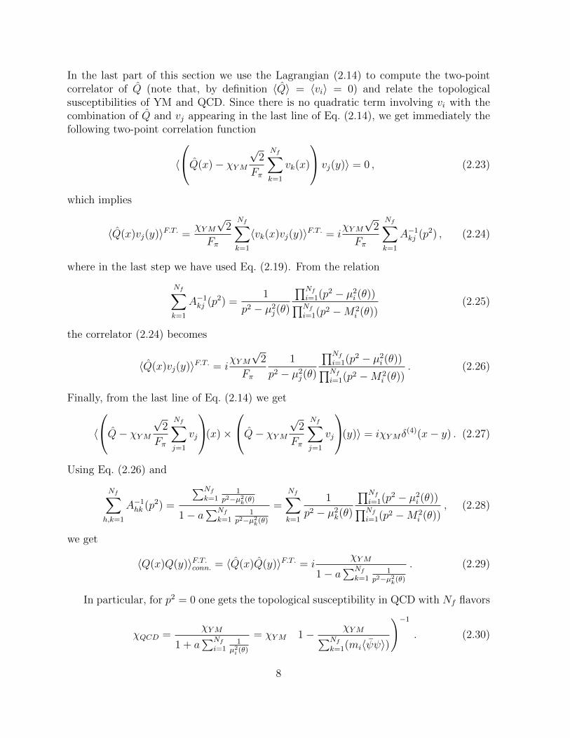
Figure 1: Solutions of V ′(φ) = 0 are given by the intersections of the curve sinφ (black) with the

straight lines (θ − φ)/ε for θ = 0, θ = π and a generic value taken to be θ = 1.58. Code color is as

follows: ε < 1 green lines, ε = 1 red lines, ε > 1 blue lines.

from which we can compute its derivatives with respect to φ

V ′

a= ε sinφ+ φ− θ ;

V ′′

a= ε cosφ+ 1

V ′′′

a= −ε sinφ ;

V ′′′′

a= −ε cosφ . (3.2)

Let us distinguish two cases:

• ε < 1

In this case V ′′ > 0 so that there can only be a single stable minimum with positivemass. This is confirmed by solving graphically the equation V ′ = 0, as illustratedin Fig. 1. At θ = 0 the minimum is at φ = 0 while at θ = π it is at φ = π. Inboth cases CP is unbroken. At 0 < θ < π (π < θ < 2π) the minimum is at some0 < φ < θ (θ < φ < 2π) and CP is explicitly broken.

• ε ≥ 1

This case is much richer. Since now V ′′ can be negative, some stationary points cancorrespond to maxima rather than minima of V . For a zero mass ground state weshould require V ′ = V ′′ = 0. But for it to be the absolute minimum we should alsohave V ′′′ = 0 and V ′′′′ > 0. However, from (3.2) we see that V ′′′ = 0 is only possibleif φ = π mod(π) and therefore (from the first and last of Eqs. (3.2)) if θ = π. Letus then consider this case in more detail.

10

Out[7]=

1 2 3 4 5 6

2

3

4

5

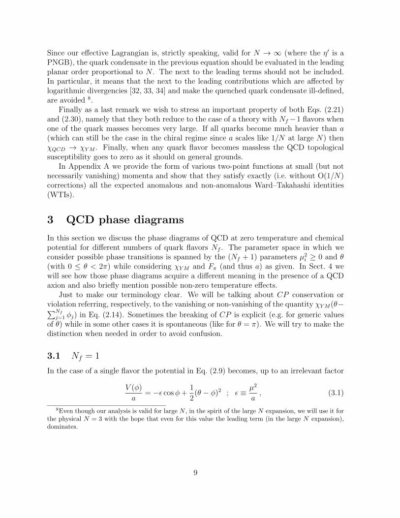
Figure 2: V (φ) of Eq. (3.1) at θ = π, and ε = 0.5 (green curve), ε = 1.0 (red) and ε = 2.0 (blue).

For θ = π there is always a stationary point at φ = π which, however, for the caseε > 1, corresponds to a maximum (V ′′ < 0). Since V is bounded from below thereshould be minima elsewhere. Indeed, for ε = 1 + δ, δ � 1, one easily finds two(degenerate) minima. For ε = 1 the three stationary points degenerate at φ = πand the stable minimum corresponds to a massless CP conserving ground state.

To make the discussion more quantitative let us assume that θ = π and that φ = π−δwhere δ is a small quantity. We can determine δ by plugging it into the first equationin (3.2) getting

δ

(δ2ε

6+ 1− ε

)= 0 . (3.3)

In this way we find again the solution δ = 0, which corresponds to a maximum,together with two stable minima related by CP (see below) at

δ± = ±√

6(ε− 1)

ε. (3.4)

This can be seen by plugging (3.4) in the second of the equations (3.2) obtainingrespectively

V ′′

a

∣∣∣δ=0

= 1− ε ;V ′′

a

∣∣∣δ±

= 2(ε− 1) . (3.5)

11

Out[25]=

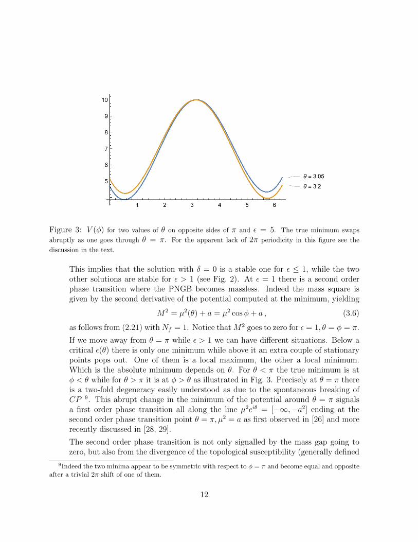
Figure 3: V (φ) for two values of θ on opposite sides of π and ε = 5. The true minimum swaps

abruptly as one goes through θ = π. For the apparent lack of 2π periodicity in this figure see the

discussion in the text.

This implies that the solution with δ = 0 is a stable one for ε ≤ 1, while the twoother solutions are stable for ε > 1 (see Fig. 2). At ε = 1 there is a second orderphase transition where the PNGB becomes massless. Indeed the mass square isgiven by the second derivative of the potential computed at the minimum, yielding

M2 = µ2(θ) + a = µ2 cosφ+ a , (3.6)

as follows from (2.21) with Nf = 1. Notice that M2 goes to zero for ε = 1, θ = φ = π.

If we move away from θ = π while ε > 1 we can have different situations. Below acritical ε(θ) there is only one minimum while above it an extra couple of stationarypoints pops out. One of them is a local maximum, the other a local minimum.Which is the absolute minimum depends on θ. For θ < π the true minimum is atφ < θ while for θ > π it is at φ > θ as illustrated in Fig. 3. Precisely at θ = π thereis a two-fold degeneracy easily understood as due to the spontaneous breaking ofCP 9. This abrupt change in the minimum of the potential around θ = π signalsa first order phase transition all along the line µ2eiθ = [−∞,−a2] ending at thesecond order phase transition point θ = π, µ2 = a as first observed in [26] and morerecently discussed in [28, 29].

The second order phase transition is not only signalled by the mass gap going tozero, but also from the divergence of the topological susceptibility (generally defined

9Indeed the two minima appear to be symmetric with respect to φ = π and become equal and oppositeafter a trivial 2π shift of one of them.

12

as the 〈Q Q〉 correlator at zero momentum) at ε = 1, θ = π. This follows fromEq. (2.30) for Nf = 1

χQCD =χYM

1 + aµ2(θ)

=χYMε cosφ

1 + ε cosφ, (3.7)

which diverges for ε = 1 at θ = φ = π.

Figs. 2 and 3 illustrate the shape of the potential for different values of ε and forθ = π or θ 6= π, respectively. Note that the potentials shown in Figs. 2 and 3 do notlook periodic in φ while they should. Indeed the potential is multi valued becauseof the log term in the effective Lagrangian (2.7) and the correct branch has to bechosen as we vary φ. Periodicity is thus restored at the expense of non-analyticitypoints (cusps) in V at particular values of φ. For instance, for θ = π (Fig. 2) thecusp are at φ = 0 mod(2π), while for a generic θ they are at θ + π mod(2π).

3.2 Nf = 2

In the case Nf = 2 with unequal masses (say, µ21 < µ2

2) the equations to be solved are

ε1 sinφ1 = ε2 sinφ2 = θ − φ1 − φ2 ; εi ≡µ2i

a. (3.8)

For θ = π the solutions are simply

φ1 = π ; φ2 = 0 or φ1 = 0 ; φ2 = π . (3.9)

The masses of the two pseudoscalar mesons can be read from Eq. (2.22) and are given by

M21,2 = a+

µ21(θ) + µ2

2(θ)

2±√a2 +

(µ2

1(θ)− µ22(θ)

2

)2

, (3.10)

valid for arbitrary θ. It is easy to check that the mass squared with the minus sign ismassless if the following condition is satisfied

a(µ22(θ) + µ2

1(θ)) =

(µ2

1(θ)− µ22(θ)

2

)2

−(µ2

1(θ) + µ22(θ)

2

)2

. (3.11)

Notice that, if both µ21,2(θ) are positive, the previous condition cannot be satisfied because

the r.h.s. is always negative, while the l.h.s. is always positive. In particular, it cannot besatisfied at θ = 0. But at θ = φ1 = π, the previous condition becomes

a(µ22 − µ2

1) = µ21µ

22 =⇒ 1

a+

1

µ22

=1

µ21

. (3.12)

This means that, if the condition

1

µ21

− 1

µ22

≥ 1

a(3.13)

13

is fulfilled, CP is unbroken because θ−φ1−φ2 = 0. Although the second solution in (3.9)conserves CP , it does not correspond to the absolute minimum and does not satisfy (3.11).

On the other hand, if µ−21 < µ−2

2 + a−1 not even the first solution in Eq. (3.9) cor-responds to a minimum and other solutions takes over. As in the case Nf = 1, let usconsider the following example. Defining

εi = µ2i /a ; ρ = ε1/ε2 ; σ = ε1 + ρ− 1 , (3.14)

one finds, to leading order in σ � 1, the two further solutions

φ1 = π − δ1 ; φ2 = δ2 ; δ1 = ±√

6σ

1− ρ3; δ2 = ρδ1 . (3.15)

In the general case the solutions can be found numerically. Fig. 4 illustrates again thethree distinct cases for θ = π, while Fig. 5 does the same for θ 6= π. We see clearly that,as in the Nf = 1 case, the critical surface µ−2

1 = µ−22 + a−1 separates the situation with a

single solution from the one with several solutions. In the latter case CP is spontaneouslybroken and the ground state jumps as we go from θ < π to θ > π. On the critical surfacethere is a massless excitation and the QCD topological susceptibility blows up.

In this generic case the phase structure resembles the Nf = 1 case. In the complexµ2

1eiθ plane (µ2

1 is the smallest mass parameter) we find a line of first order transitionsalong the negative axis ending on a second order transition point where one mass goesto zero. The position of the second order point depends on the other parameters (massratios, a). We can also see this structure in the complex detµ2 plane, as discussed in thenext subsection.

Let us close with a short discussion of the peculiarities of the equal mass case, µ21 =

µ22 = µ2. In this case the condition (3.13) cannot be satisfied except, asymptotically, if we

send µ2/a to zero. In other words, as discussed in [29], the first order phase transition linenow extends over the whole negative real axis terminating at the origin. However, beforejumping too quickly to this conclusion we should observe that the potential becomes veryflat for small µ2/a, so much that it develops a flat direction at O(µ2/a). This continuousvacuum degeneracy is lifted at O((µ2/a)2) so that the CP violating minimum is foundto lie O((µ2/a)2) below the CP conserving one. The existence of this quasi-flat directionand its lifting to O(m2) was first pointed out in [24] and further discussed in [29]. Ingeneral, O(m2) corrections are not included in effective Lagrangians like (2.1) but, in thecontext of our double limit m/Λ → 0, N → ∞ with mN/Λ fixed (recall a ∼ Λ2/N),the split in the potential between the two vacua is of order Λ4(mN/Λ)2 while the O(m2)corrections we are ignoring are at least a factor 1/N lower. We can thus conclude that,above a sufficiently large N , CP is broken for two equal mass flavors 10.

10We thank Z. Komargodski for having raised with us the issue of flat directions and for useful corre-spondence about it.

14

In[1]:= ContourPlot[{Sin[x] ⩵ 2 * Sin[y], (Pi - x - y) == Sin[x]}, {x, 0, 2 * Pi}, {y, -2, 2}]

Out[1]=

0 1 2 3 4 5 6-2

-1

0

1

2

In[2]:= ContourPlot[{0.5 * Sin[x] ⩵ 2 * Sin[y], (Pi - x - y) == 0.5 * Sin[x]},{x, 0, 2 * Pi}, {y, -2, 2}]

Out[2]=

0 1 2 3 4 5 6-2

-1

0

1

2

In[1]:= ContourPlot[{Sin[x] ⩵ 2 * Sin[y], (Pi - x - y) == Sin[x]}, {x, 0, 2 * Pi}, {y, -2, 2}]

Out[1]=

0 1 2 3 4 5 6-2

-1

0

1

2

In[2]:= ContourPlot[{0.5 * Sin[x] ⩵ 2 * Sin[y], (Pi - x - y) == 0.5 * Sin[x]},{x, 0, 2 * Pi}, {y, -2, 2}]

Out[2]=

0 1 2 3 4 5 6-2

-1

0

1

2

In[3]:= ContourPlot[{2 * Sin[x] / 3 ⩵ 2 * Sin[y], (Pi - x - y) == 2 * Sin[x] / 3},{x, 0, 2 * Pi}, {y, -2, 2}]

Out[3]=

0 1 2 3 4 5 6-2

-1

0

1

2

2 N_F=2_slns.new.nb

φ2 φ2

φ2

φ1

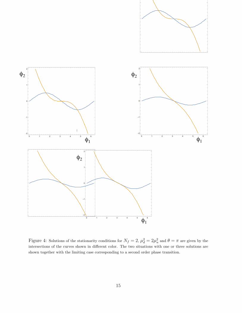
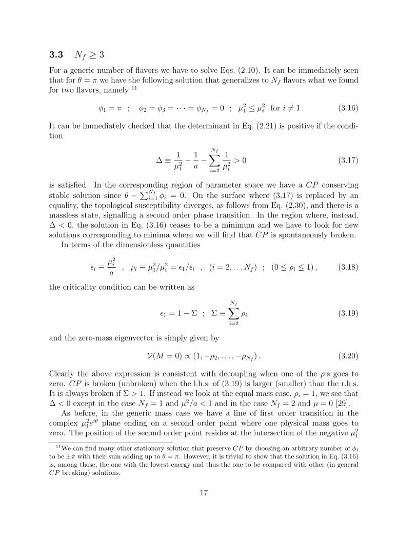
φ1φ1

Figure 4: Solutions of the stationarity conditions for Nf = 2, µ2d = 2µ2

u and θ = π are given by the

intersections of the curves shown in different color. The two situations with one or three solutions are

shown together with the limiting case corresponding to a second order phase transition.

15

In[1]:= ContourPlot[{Sin[x] ⩵ 2 * Sin[y], (Pi - 0.1 - x - y) == Sin[x]},{x, 0, 2 * Pi}, {y, -2, 2}]

Out[1]=

0 1 2 3 4 5 6-2

-1

0

1

2

In[2]:= ContourPlot[{Sin[x] ⩵ 2 * Sin[y], (Pi + 0.1 - x - y) == Sin[x]},{x, 0, 2 * Pi}, {y, -2, 2}]

Out[2]=

0 1 2 3 4 5 6-2

-1

0

1

2

In[1]:= ContourPlot[{Sin[x] ⩵ 2 * Sin[y], (Pi - 0.1 - x - y) == Sin[x]},{x, 0, 2 * Pi}, {y, -2, 2}]

Out[1]=

0 1 2 3 4 5 6-2

-1

0

1

2

In[2]:= ContourPlot[{Sin[x] ⩵ 2 * Sin[y], (Pi + 0.1 - x - y) == Sin[x]},{x, 0, 2 * Pi}, {y, -2, 2}]

Out[2]=

0 1 2 3 4 5 6-2

-1

0

1

2

φ2 φ2

φ1 φ1

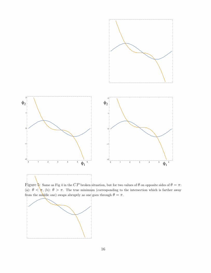
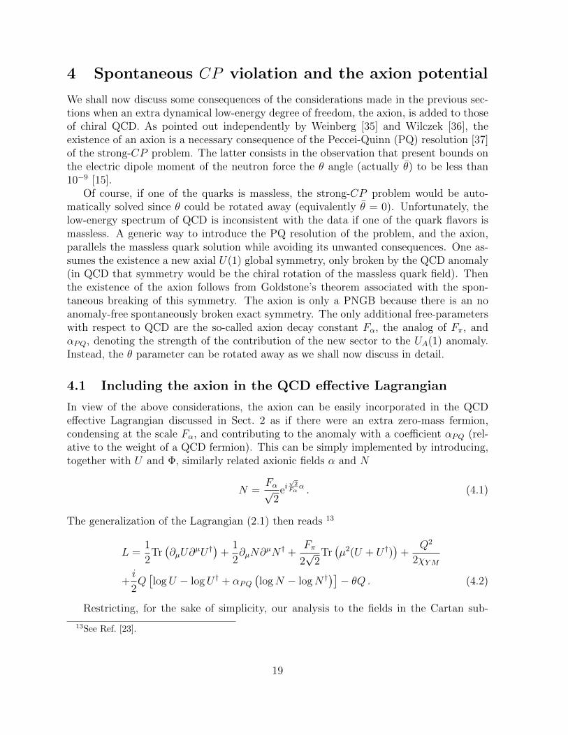
Figure 5: Same as Fig 4 in the CP broken situation, but for two values of θ on opposite sides of θ = π:

(a): θ < π, (b): θ > π. The true minimum (corresponding to the intersection which is farther away

from the middle one) swaps abruptly as one goes through θ = π.

16

3.3 Nf ≥ 3

For a generic number of flavors we have to solve Eqs. (2.10). It can be immediately seenthat for θ = π we have the following solution that generalizes to Nf flavors what we foundfor two flavors, namely 11

φ1 = π ; φ2 = φ3 = · · · = φNf = 0 ; µ21 ≤ µ2

i for i 6= 1 . (3.16)

It can be immediately checked that the determinant in Eq. (2.21) is positive if the condi-tion

∆ ≡ 1

µ21

− 1

a−

Nf∑

i=2

1

µ2i

> 0 (3.17)

is satisfied. In the corresponding region of parameter space we have a CP conserving

stable solution since θ −∑Nfi=1 φi = 0. On the surface where (3.17) is replaced by an

equality, the topological susceptibility diverges, as follows from Eq. (2.30), and there is amassless state, signalling a second order phase transition. In the region where, instead,∆ < 0, the solution in Eq. (3.16) ceases to be a minimum and we have to look for newsolutions corresponding to minima where we will find that CP is spontaneously broken.

In terms of the dimensionless quantities

εi ≡µ2i

a, ρi ≡ µ2

1/µ2i = ε1/εi , (i = 2, . . . Nf ) ; (0 ≤ ρi ≤ 1) , (3.18)

the criticality condition can be written as

ε1 = 1− Σ ; Σ ≡Nf∑

i=2

ρi (3.19)

and the zero-mass eigenvector is simply given by

V(M = 0) ∝ (1,−ρ2, . . . ,−ρNf ) . (3.20)

Clearly the above expression is consistent with decoupling when one of the ρ’s goes tozero. CP is broken (unbroken) when the l.h.s. of (3.19) is larger (smaller) than the r.h.s.It is always broken if Σ > 1. If instead we look at the equal mass case, ρi = 1, we see that∆ < 0 except in the case Nf = 1 and µ2/a < 1 and in the case Nf = 2 and µ = 0 [29].

As before, in the generic mass case we have a line of first order transition in thecomplex µ2

1eiθ plane ending on a second order point where one physical mass goes to

zero. The position of the second order point resides at the intersection of the negative µ21

11We can find many other stationary solution that preserve CP by choosing an arbitrary number of φito be ±π with their sum adding up to θ = π. However, it is trivial to show that the solution in Eq. (3.16)is, among those, the one with the lowest energy and thus the one to be compared with other (in generalCP breaking) solutions.

17

line with the critical hyper surface and therefore depends on the other parameters (massratios, a).

We end this section giving a definition of the critical hypersurface in terms of thequantity D ≡ det(µ2/a2) = det(ε), where, however, µ2 is now the matrix introducedin (2.1) after having absorbed the θ angle by a chiral rotation 12. The critical value ofD, Dc, is negative (corresponding to θ = − argD = ±π) and its absolute value dependsonly on the ratios ρi introduced earlier. Indeed the condition for CP violation can beexpressed as follows

|D| > |Dc| ; |D1/Nfc | = (1− Σ)Π−1/Nf ; Π =

Nf∏

i=2

ρi . (3.21)

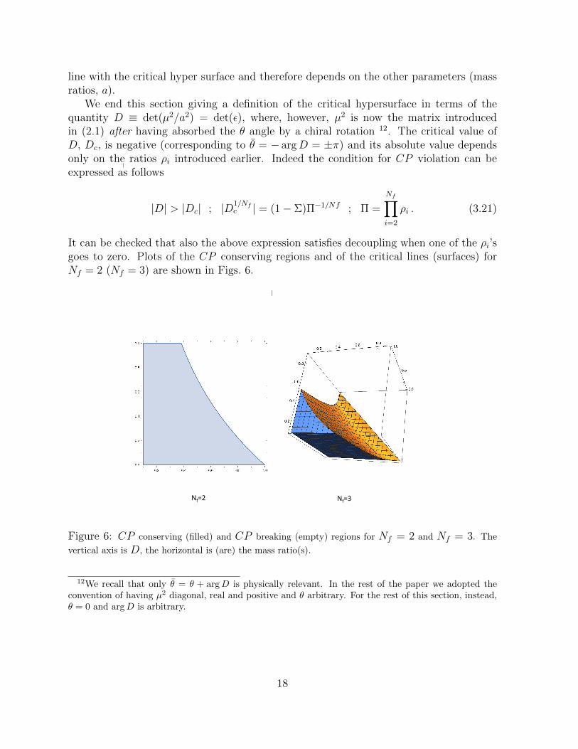
It can be checked that also the above expression satisfies decoupling when one of the ρi’sgoes to zero. Plots of the CP conserving regions and of the critical lines (surfaces) forNf = 2 (Nf = 3) are shown in Figs. 6.

RegionPlot3D[z^(1 / 3) - (1 - y - x) * (y * x)^(-1 / 3) < 0,{z, 0, 1}, {y, 0.1, 1}, {x, 0.1, 1}, PlotPoints → 35, PlotRange → All]

RegionPlot[y - (1 - x) * (x)^(-1 / 2) < 0, {x, 0.1, 1}, {y, 0, 1}]

(* Nf = 2. The vertical coordinate is det^{1/2}*)

2 RegionPlots.Nf=2,3.nb

RegionPlot3D[z^(1 / 3) - (1 - y - x) * (y * x)^(-1 / 3) < 0,{z, 0, 1}, {y, 0.1, 1}, {x, 0.1, 1}, PlotPoints → 35, PlotRange → All]

RegionPlot[y - (1 - x) * (x)^(-1 / 2) < 0, {x, 0.1, 1}, {y, 0, 1}]

(* Nf = 2. The vertical coordinate is det^{1/2}*)

2 RegionPlots.Nf=2,3.nb

Nf=2 Nf=3

Figure 6: CP conserving (filled) and CP breaking (empty) regions for Nf = 2 and Nf = 3. The

vertical axis is D, the horizontal is (are) the mass ratio(s).

12We recall that only θ = θ + argD is physically relevant. In the rest of the paper we adopted theconvention of having µ2 diagonal, real and positive and θ arbitrary. For the rest of this section, instead,θ = 0 and argD is arbitrary.

18

4 Spontaneous CP violation and the axion potential

We shall now discuss some consequences of the considerations made in the previous sec-tions when an extra dynamical low-energy degree of freedom, the axion, is added to thoseof chiral QCD. As pointed out independently by Weinberg [35] and Wilczek [36], theexistence of an axion is a necessary consequence of the Peccei-Quinn (PQ) resolution [37]of the strong-CP problem. The latter consists in the observation that present bounds onthe electric dipole moment of the neutron force the θ angle (actually θ) to be less than10−9 [15].

Of course, if one of the quarks is massless, the strong-CP problem would be auto-matically solved since θ could be rotated away (equivalently θ = 0). Unfortunately, thelow-energy spectrum of QCD is inconsistent with the data if one of the quark flavors ismassless. A generic way to introduce the PQ resolution of the problem, and the axion,parallels the massless quark solution while avoiding its unwanted consequences. One as-sumes the existence a new axial U(1) global symmetry, only broken by the QCD anomaly(in QCD that symmetry would be the chiral rotation of the massless quark field). Thenthe existence of the axion follows from Goldstone’s theorem associated with the spon-taneous breaking of this symmetry. The axion is only a PNGB because there is an noanomaly-free spontaneously broken exact symmetry. The only additional free-parameterswith respect to QCD are the so-called axion decay constant Fα, the analog of Fπ, andαPQ, denoting the strength of the contribution of the new sector to the UA(1) anomaly.Instead, the θ parameter can be rotated away as we shall now discuss in detail.

4.1 Including the axion in the QCD effective Lagrangian

In view of the above considerations, the axion can be easily incorporated in the QCDeffective Lagrangian discussed in Sect. 2 as if there were an extra zero-mass fermion,condensing at the scale Fα, and contributing to the anomaly with a coefficient αPQ (rel-ative to the weight of a QCD fermion). This can be simply implemented by introducing,together with U and Φ, similarly related axionic fields α and N

N =Fα√

2ei√2

Fαα . (4.1)

The generalization of the Lagrangian (2.1) then reads 13

L =1

2Tr(∂µU∂

µU †)

+1

2∂µN∂

µN † +Fπ

2√

2Tr(µ2(U + U †)

)+

Q2

2χYM

+i

2Q[logU − logU † + αPQ

(logN − logN †

)]− θQ . (4.2)

Restricting, for the sake of simplicity, our analysis to the fields in the Cartan sub-

13See Ref. [23].

19

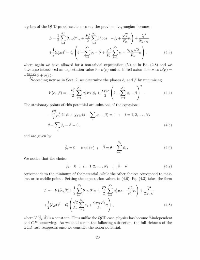
algebra of the QCD pseudoscalar mesons, the previous Lagrangian becomes

L =1

2

Nf∑

i=1

∂µvi∂µvi +

F 2π

2

Nf∑

i=1

µ2i cos

(−φi +

√2

Fπvi

)+

Q2

2χYM

+1

2(∂µα)2 −Q

θ −

Nf∑

i=1

φi − β +

√2

Fπ

Nf∑

i=1

vi +αPQ√

2

Fασ

, (4.3)

where again we have allowed for a non-trivial expectation 〈U〉 as in Eq. (2.8) and wehave also introduced an expectation value for α(x) and a shifted axion field σ as α(x) =

−αPQ√

2

Fαβ + σ(x).

Proceeding now as in Sect. 2, we determine the phases φi and β by minimizing

V (φi, β) = −F2π

2

Nf∑

i=1

µ2i cosφi +

χYM2

θ −

Nf∑

i=1

φi − β

2

. (4.4)

The stationary points of this potential are solutions of the equations

−F2π

2µ2i sinφi + χYM(θ −

∑

i

φi − β) = 0 ; i = 1, 2, . . . , Nf

θ −∑

i

φi − β = 0 , (4.5)

and are given by

φi = 0 mod (π) ; β = θ −Nf∑

i=1

φi . (4.6)

We notice that the choice

φi = 0 ; i = 1, 2, . . . , Nf ; β = θ (4.7)

corresponds to the minimum of the potential, while the other choices correspond to max-ima or to saddle points. Setting the expectation values to (4.6), Eq. (4.3) takes the form

L = −V (φi, β) +1

2

Nf∑

i=1

∂µvi∂µvi +

F 2π

2

Nf∑

i=1

µ2i cos

(√2

Fπvi

)+

Q2

2χYM

+1

2(∂µσ)2 −Q

√

2

Fπ

Nf∑

i=1

vi +αPQ√

2

Fασ

, (4.8)

where V (φi, β) is a constant. Thus unlike the QCD case, physics has become θ-independentand CP conserving. As we shall see in the following subsection, the full richness of theQCD case reappears once we consider the axion potential.

20

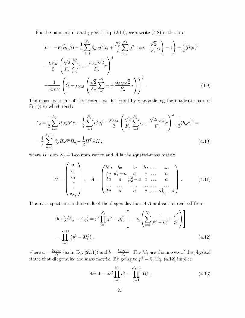
For the moment, in analogy with Eq. (2.14), we rewrite (4.8) in the form

L = −V (φi, β) +1

2

Nf∑

i=1

∂µvi∂µvi +

F 2π

2

Nf∑

i=1

µ2i

(cos

(√2

Fπvi

)− 1

)+

1

2(∂µσ)2

−χYM2

√

2

Fπ

Nf∑

i=1

vi +αPQ√

2

Fασ

2

+1

2χYM

Q− χYM

√

2

Fπ

Nf∑

i=1

vi +αPQ√

2

Fασ

2

. (4.9)

The mass spectrum of the system can be found by diagonalizing the quadratic part ofEq. (4.9) which reads

L2 =1

2

Nf∑

i=1

∂µvi∂µvi −

1

2

Nf∑

i=1

µ2i v

2i −

χYM2

√

2

Fπ

Nf∑

i=1

vi +

√2αPQFα

σ

2

+1

2(∂µσ)2 =

=1

2

Nf+1∑

a=1

∂µHa∂µHa −

1

2HTAH , (4.10)

where H is an Nf + 1-column vector and A is the squared-mass matrix

H =

σv1

v2

··vNf

; A =

b2a ba ba ba . . . baba µ2

1 + a a a . . . aba a µ2

2 + a a . . . a. . . . . . . . . . . . . . . . . .ba a a a . . . µ2

Nf+ a

. (4.11)

The mass spectrum is the result of the diagonalization of A and can be read off from

det(p2δij − Aij

)= p2

Nf∏

i=1

(p2 − µ2i )

1− a

Nf∑

i=1

1

p2 − µ2i

+b2

p2

=

Nf+1∏

i=1

(p2 −M2

i

), (4.12)

where a = 2χYMF 2π

(as in Eq. (2.11)) and b =FπαPQFα

. The Mi are the masses of the physical

states that diagonalize the mass matrix. By going to p2 = 0, Eq. (4.12) implies

detA = ab2

Nf∏

i=1

µ2i =

Nf+1∏

j=1

M2j , (4.13)

21

where the product on the r.h.s. includes the axion as well as the Cartan PNGB masses.Note that, unlike the non-axionic case, for non-vanishing mi, a and b, this determinant isalways positive implying no massless state (and indeed a non-tachyonic spectrum). Thiswould have also been the case had we considered QCD with one massless flavor (in thatcase b = 1). In particular, for small b, the mass of the axion is given by looking for a zeroat small p2 of the term in square brackets in Eq. (4.12). Neglecting p2 with respect to µ2

i

one obtains

M2axion =

b2

1a

+∑Nf

i=11µ2i

. (4.14)

This reduces to the usual expression for the axion mass [35, 38] in the limit a, µ2s � µ2

u,d.Alternatively, using Eq. (2.30) and the definition of b, we can write

M2axion =

2α2PQ

F 2α

χQCD , (4.15)

another formula often used in the literature (see e.g. Ref. [39]).Finally, from the term in the last line of Eq. (4.9) and the matrix definition in Eq. (4.10)

we get (having 〈Q〉 = 0) the following two-point correlation function

〈Q(x)Q(y)〉F.T. = iχYMp2∏Nf

i=1(p2 − µ2i )∏Nf+1

i=1 (p2 −M2i )

=iχYM[

1− a(∑Nf

i=11

p2−µ2i+ b2

p2

)] , (4.16)

that vanishes at p2 = 0 signalling that the topological susceptibility in a theory whereQCD is “augmented” by another sector that includes the axion, is zero consistently withthe fact that the dependence on the θ parameter disappears.

For the physically interesting case we have to take b� 1 so that the spectrum shouldcontain a very light pseudo-scalar, the physical axion, which is the original field σ up to anO(b) admixture of PNGBs. This is all well known. We will now discuss how things takean interesting turn when we go from properties of the spectrum (i.e. of small fluctuationsaround the minimum of V ) to those of the full potential at a finite distance from itsminimum.

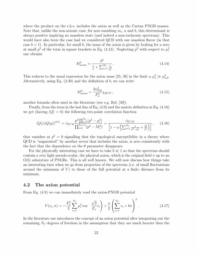
4.2 The axion potential

From Eq. (4.9) we can immediately read the axion-PNGB potential

V (vi, σ) = −F2π

2

Nf∑

i=1

µ2i cos

(√2

Fπvi

)+a

2

Nf∑

i=1

vi + bσ

2

. (4.17)

In the literature one introduces the concept of an axion potential after integrating out theremaining Nf degrees of freedom in the assumption that they are much heavier then the

22

axion. In principle this requires diagonalizing the mass matrix so as to be in position ofidentifying the lowest lying state, the physical axion that will be a mixture of σ and thevi. In the limit of very small b, which is where physics lies, one can neglect these mixingsand identify σ with the axion modulo some exceptional cases to be discussed below.

For the physically interesting case of two light flavors the axion potential was firstderived in [17] under the assumption µ2

1, µ22 � a with the result [30]

Vaxion(σ) = −F2π

2

√(µ2

1 + µ22)2 − 4µ2

1µ22 sin2

(αPQσ√

2Fα

)+ O(µ2

i /a) , (4.18)

which for Nf = 1 simply becomes

Vaxion(σ) = −F2π

2µ2 cos

(√2αPQσ

Fα

)+ O(µ2/a) . (4.19)

We see, however, that by having considered the axion potential at a generic value ofσ we have effectively recovered, mutatis mutandis, the situation discussed in QCD atfixed θ. This is why the discussion of Sect. 3 becomes very relevant here. Indeed, theprevious analysis shows that, precisely around σ = πFα√

2αPQ, some PNGB mass can become

arbitrarily small. In this case integrating out the PNGB fields is no longer justified anda more careful analysis is needed. In other cases the naive solution for the vi correspondsto a maximum and it has to be replaced with the right solution. The rest of this sectionis devoted to such an analysis for different numbers of quark flavors.

In the following, for simplicity of notation, we shall denote by ϕi and ζ the dimen-

sionless quantities −√

2Fπvi and

√2αPQFα

σ, respectively. In this notation the potential (4.17)simply reads

2F−2π V (ζ, ϕi) = −

Nf∑

i=1

µ2i cosϕi +

a

2

Nf∑

i=1

ϕi − ζ

2

. (4.20)

4.2.1 Nf = 1

The potential V (ζ, ϕ) has two distinct stationary points, one at ζ = ϕ = 0 and one atζ = ϕ = π. The first is a true minimum, the second a saddle point. Let us now considerthe stationary points in ϕ at fixed ζ in order to compute Vaxion(ζ), distinguishing threecases (looking at Fig. 1 can help following the discussion).

• µ2/a < 1. In this case there is a single stationary point at ϕ(ζ) ≤ ζ which growsmonotonically with ζ interpolating between the two stationary points of V . In thiscase the potential (4.19) is easily recovered. At ζ = π the potential is smooth andreaches a maximum lying µ2F 2

π above the absolute minimum. One can easily checkthat, for µ2/a not too close to 1, the mass of the PNGB is always much larger thanthe scale of variation of the axion potential so that integrating out that degree offreedom is justified. We shall discuss separately the case |1− µ2/a| � 1.

23

• µ2/a > 1. In this case, as one varies ζ from 0 to π, ϕ(ζ) remains always smallerthan ζ. Actually, above a value of ζ that depends on µ2/a, new stationary pointsin ϕ (lying above ϕ = π) appear but they have higher energy. This is nothing butthe situation we have described and discussed around Fig. 3. In particular, as weapproach ζ = π, ϕ approaches a finite value smaller than π and behaving as πa/µ2

for µ2/a � 1. Precisely at ζ = π this minimum becomes degenerate with one atϕ > π which, upon a shift by 2π is just its CP transformed. Again, for µ2/a not tooclose to 1, integrating out the PNGB appears fully justified but, instead of (4.19),we get

Vaxion(σ) =1

2χYM

(√2αPQσ

Fα

)2

+ O(a/µ2) , (4.21)

where for a moment we have reintroduced the canonical σ field. In particular,the axion mass is now controlled by a rather than by µ2. At the boundary of itsperiodicity interval Vaxion now reaches its maximal value 1

2χYMπ

2 � µ2F 2π (in the

small-a limit). Furthermore, at that point its first derivative is non-vanishing (andpositive) and, since the potential is periodic, its first derivative will be discontinuous,giving a spike at ζ = π. This, of course, is related to the fact that the solution forϕ jumps abruptly as we go through θ = π (see again Fig. 3).

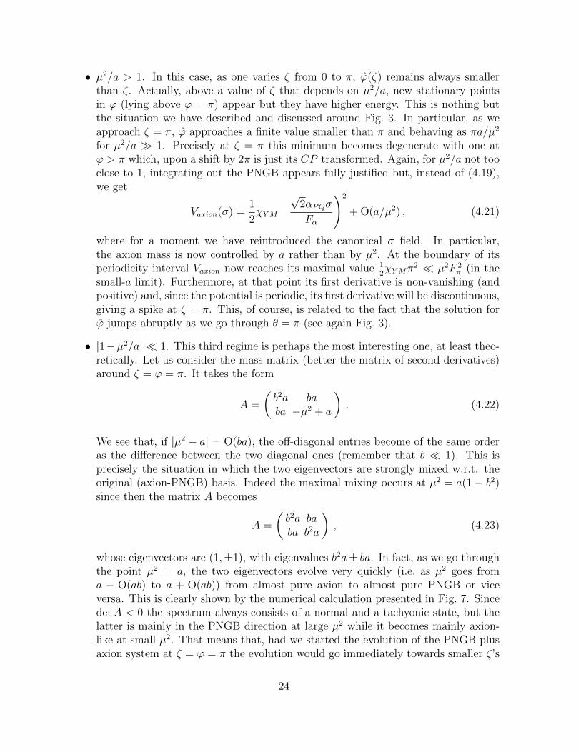
• |1−µ2/a| � 1. This third regime is perhaps the most interesting one, at least theo-retically. Let us consider the mass matrix (better the matrix of second derivatives)around ζ = ϕ = π. It takes the form

A =

(b2a baba −µ2 + a

). (4.22)

We see that, if |µ2 − a| = O(ba), the off-diagonal entries become of the same orderas the difference between the two diagonal ones (remember that b � 1). This isprecisely the situation in which the two eigenvectors are strongly mixed w.r.t. theoriginal (axion-PNGB) basis. Indeed the maximal mixing occurs at µ2 = a(1− b2)since then the matrix A becomes

A =

(b2a baba b2a

), (4.23)

whose eigenvectors are (1,±1), with eigenvalues b2a± ba. In fact, as we go throughthe point µ2 = a, the two eigenvectors evolve very quickly (i.e. as µ2 goes froma − O(ab) to a + O(ab)) from almost pure axion to almost pure PNGB or viceversa. This is clearly shown by the numerical calculation presented in Fig. 7. SincedetA < 0 the spectrum always consists of a normal and a tachyonic state, but thelatter is mainly in the PNGB direction at large µ2 while it becomes mainly axion-like at small µ2. That means that, had we started the evolution of the PNGB plusaxion system at ζ = ϕ = π the evolution would go immediately towards smaller ζ’s

24

if µ2 < a while, for µ2 > a, it would first roll down to the true minimum in ϕ andonly then will roll down towards ζ = 0, ϕ = 0.

It is also quite clear that in this particular range of µ2/a and ζ it is not possible todescribe the system only in terms of a Vaxion(ζ) since the other degree of freedom isas light as the axion itself. Only a description in terms of a V (ζ, ϕ) is fully adequate.

4.2.2 Nf ≥ 2 and discussion

The real world has two very light quarks, u and d, a light one, s, and three heavy quarks.The latter play no role in our discussion. Thus the case of physical interest is Nf = 2 or3. Also, at zero temperature, the quantitative solution of the U(1) problem requires [7],[8] µ2

u < µ2d << µ2

s < a. The ratios µ2u : µ2

d : µ2s : a are about 1 : 2 : 40 : 18. In what

follows we shall use these numbers together with the results we obtained from the large-N effective action approach, even though in the real world N = 3. The success of thelarge-N solution to the U(1) problem suggests that, at least in this sector, the large-Nexpansion converges quite fast.

We should keep in mind, however, that, while quark mass ratios are expected to beconstant below the QCD deconfining temperature (they depend on phenomena occurringat the electroweak-breaking scale), the temperature dependence of χYM could possiblydiffer from that of the quark condensate meaning a possible (strong?) T -dependence ofµ2/a. An increase of that ratio by an order of magnitude would bring us inside the CPbroken region. The available lattice measurements [40, 41, 42] do not seem to favor thispossibility. We defer further comments on this issue to the conclusion section.

In the following we will consider therefore the case of two or three quark flavors of dif-ferent masses and allow for arbitrary ratios µ2

i /a. The situation is now more involved thanin the Nf = 1 case, but qualitatively similar. The stationary points of the potential (4.20)are

ζ = 0, π mod (2π) ; ϕi = 0, π mod (2π) ;∑

ϕi = ζ . (4.24)

The absolute minimum is as usual the trivial one ζ = ϕi = 0. In general it is legitimateto integrate out the PNGB degrees of freedom by minimizing their potential at fixed ζand then insert the solution ϕi(ζ) in V (ζ, ϕi). If µ2

i � a this can be easily done. In thetwo-flavor case this gives the result (4.18). In the three-flavor case recalling that

sinφs = µ2u/µ

2s sinφu � sinφu , (4.25)

we see that the result (4.18) still holds up to corrections O(µ2u,d/µ

2s). This is indeed the

result used in the literature.What happens if, for some physical reason, χYM drops so fast with T that a becomes of

order µ2u,d or even smaller? We can understand the situation by considering what happens

at the saddle point corresponding to

ζ = ϕu = π , ϕd = ϕs = 0 . (4.26)

25

-0.5 0.5 1.0 1.5 2.0 2.5

-1.5

-1.0

-0.5

0.5

1.0

1.5

-0.5 0.5 1.0 1.5 2.0 2.5

0.2

0.4

0.6

0.8

1.0

(a)

(b)

Figure 7: Nf = 1. (a) Evolution of the two eigenvalues of (4.22) for b = 0.1 as one varies µ2/a. The

lower eigenvalue is tachyonic. (b) Projections of the two corresponding eigenvectors along the PNGB

direction. Maximal mixing occurs in the vicinity of the critical point µ2/a = 1.

We have seen in Sects. 3.2 and 3.3 that the condition for having a massless boson (inthe absence of the axion) is

1

µ2u

=1

a+

1

µ2d

+1

µ2s

∼ 1

a+

1

µ2d

⇒ a(µ2d − µ2

u) = µ2uµ

2d . (4.27)

Precisely around this point we expect a large mixing to occur between the would-be mass-less PNGB and the axion and, as one goes through that region, we expect the tachyonicboson to change its dominant component from axionic to mesonic.

This is indeed fully supported by the numerical results shown in Figs. 7 and 8 forNf = 1 and Nf = 2, respectively. We have solved, using Mathematica, the minimizationconditions at fixed ζ and reconstructed this way the axion potential (see Fig. 9). We thenclearly see that, while at small µ2

u,d/a the potential has a regular maximum around ζ = π

26

-0.5 0.5 1.0 1.5

-1

1

2

3

0.4 0.5 0.6 0.7

-0.2

-0.1

0.1

0.2

(a)

(b)

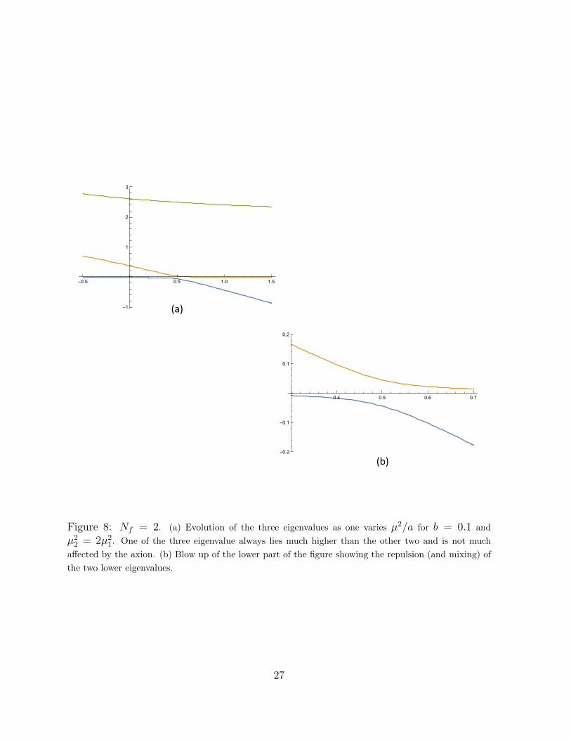
Figure 8: Nf = 2. (a) Evolution of the three eigenvalues as one varies µ2/a for b = 0.1 and

µ22 = 2µ2

1. One of the three eigenvalue always lies much higher than the other two and is not much

affected by the axion. (b) Blow up of the lower part of the figure showing the repulsion (and mixing) of

the two lower eigenvalues.

27

-3 -2 -1 1 2 3

0.1

0.2

0.3

0.4

0.5

0.6

0.7

-3 -2 -1 1 2 3

0.1

0.2

0.3

0.4

0.5

0.6

0.7

-3 -2 -1 1 2 3

0.1

0.2

0.3

0.4

0.5

0.6

0.7

-3 -2 -1 1 2 3

0.1

0.2

0.3

0.4

0.5

0.6

0.7

-3 -2 -1 1 2 3

0.1

0.2

0.3

0.4

0.5

0.6

0.7

-3 -2 -1 1 2 3

0.1

0.2

0.3

0.4

0.5

0.6

0.7

-3 -2 -1 1 2 3

0.1

0.2

0.3

0.4

0.5

0.6

0.7

-3 -2 -1 1 2 3

0.1

0.2

0.3

0.4

0.5

0.6

0.7

-3 -2 -1 1 2 3

0.1

0.2

0.3

0.4

0.5

0.6

0.7

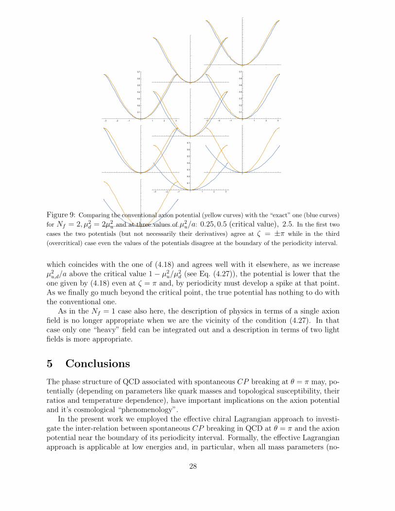
Figure 9: Comparing the conventional axion potential (yellow curves) with the “exact” one (blue curves)

for Nf = 2, µ2d = 2µ2

u and at three values of µ2u/a: 0.25, 0.5 (critical value), 2.5. In the first two

cases the two potentials (but not necessarily their derivatives) agree at ζ = ±π while in the third

(overcritical) case even the values of the potentials disagree at the boundary of the periodicity interval.

which coincides with the one of (4.18) and agrees well with it elsewhere, as we increaseµ2u,d/a above the critical value 1− µ2

u/µ2d (see Eq. (4.27)), the potential is lower that the

one given by (4.18) even at ζ = π and, by periodicity must develop a spike at that point.As we finally go much beyond the critical point, the true potential has nothing to do withthe conventional one.

As in the Nf = 1 case also here, the description of physics in terms of a single axionfield is no longer appropriate when we are the vicinity of the condition (4.27). In thatcase only one “heavy” field can be integrated out and a description in terms of two lightfields is more appropriate.

5 Conclusions

The phase structure of QCD associated with spontaneous CP breaking at θ = π may, po-tentially (depending on parameters like quark masses and topological susceptibility, theirratios and temperature dependence), have important implications on the axion potentialand it’s cosmological “phenomenology”.

In the present work we employed the effective chiral Lagrangian approach to investi-gate the inter-relation between spontaneous CP breaking in QCD at θ = π and the axionpotential near the boundary of its periodicity interval. Formally, the effective Lagrangianapproach is applicable at low energies and, in particular, when all mass parameters (no-

28

tably quark masses) are small with respect to the QCD scale, Λ. We also look at thelarge-N limit in which we can have ratios of quark masses to Λ small but still much largerthen 1/N . This allows us to identify and reliably investigate the existence, at θ = π, of asecond order phase transition point on the hypersurface dividing the region in parametersspace where CP is spontaneously broken from the one where it is not. The second orderpoint is characterized by one of the PNGB mass going to zero and by the topologicalsusceptibility (which can be seen as the order parameter) to diverge.

For generic masses the phase structure of QCD reveals a line of first order transitions,associated with spontaneous CP breaking at θ = π, along the negative real axis in thecomplex µ2

1eiθ mass plane (µ1 being the lowest quark mass). The first order line extends

all the way from −∞ to the second order point without reaching the chiral point at theorigin. The position of the second order transition depends on all other parameters (massratios and the susceptibility related parameter we called a). A similar phase structure isobtained by working in the complex quark-mass-determinant plane.

It is the existence of this second order point which has the most dramatic effect on theaxion potential. Clearly, upon introducing the axionic field into the effective Lagrangianthere is no more a θ dependence and no strong-CP breaking. However, precisely aroundthe point in parameter space (quark masses and topological susceptibility) where, in theabsence of the axion, the condition for having a zero mass boson is met, we find largemixing between the would be massless particle and the axion. In this region one cannotintegrate out all the PNGB since one of them becomes very light with a mass of the orderof the axion mass. Hence, in this region, the notion of an axionic potential which dependson just the axion field (obtained upon integration out all the PNGB) is not viable andshould be replaced by a potential which depends on the two above mentioned light degreesof freedom as discussed in Sect. 4. This potential is obtained upon integrating out all theother much heavier PNGBs.

Given the actual physical numerical values of the parameters (for Nf = 2 and Nf = 3)we see that, at zero temperature, we are not in the region of the parameter space wherethe concept of an axion potential and the derived result for the axion mass should bemodified. However, if, as we raise the temperature while staying below the deconfinementtransition (which for QCD is not a sharp transition), the corresponding YM topologicalsusceptibility (and hence the parameter a) drops faster with the temperature than thequark condensate so as to allow µ2/a to increase by about an order of magnitude, we willenter into this intriguing region (see Fig. 10).

It seems, however, that lattice calculations (see e.g. [40, 41, 42] as well as [43, 44])show a rather mild T -dependence of both χYM and the quenched chiral condensate witha sharp drop (but not necessarily vanishing) of both above a similar value of T . Theredoes not seem to be a clean window in which µ2/a increases by the above-mentioned orderof magnitude. It would be desirable to have detailed lattice data on both χYM and theplanar chiral condensate by a single group using the same Montecarlo configurations. Itwould be particularly interesting to study the pure number χYM/〈mψψ〉 in the vicinityof the above-mentioned drop and also check its N -dependence (expected to be 1/N).

An obviously related issue is whether there is a critical temperature Ttop above which

29

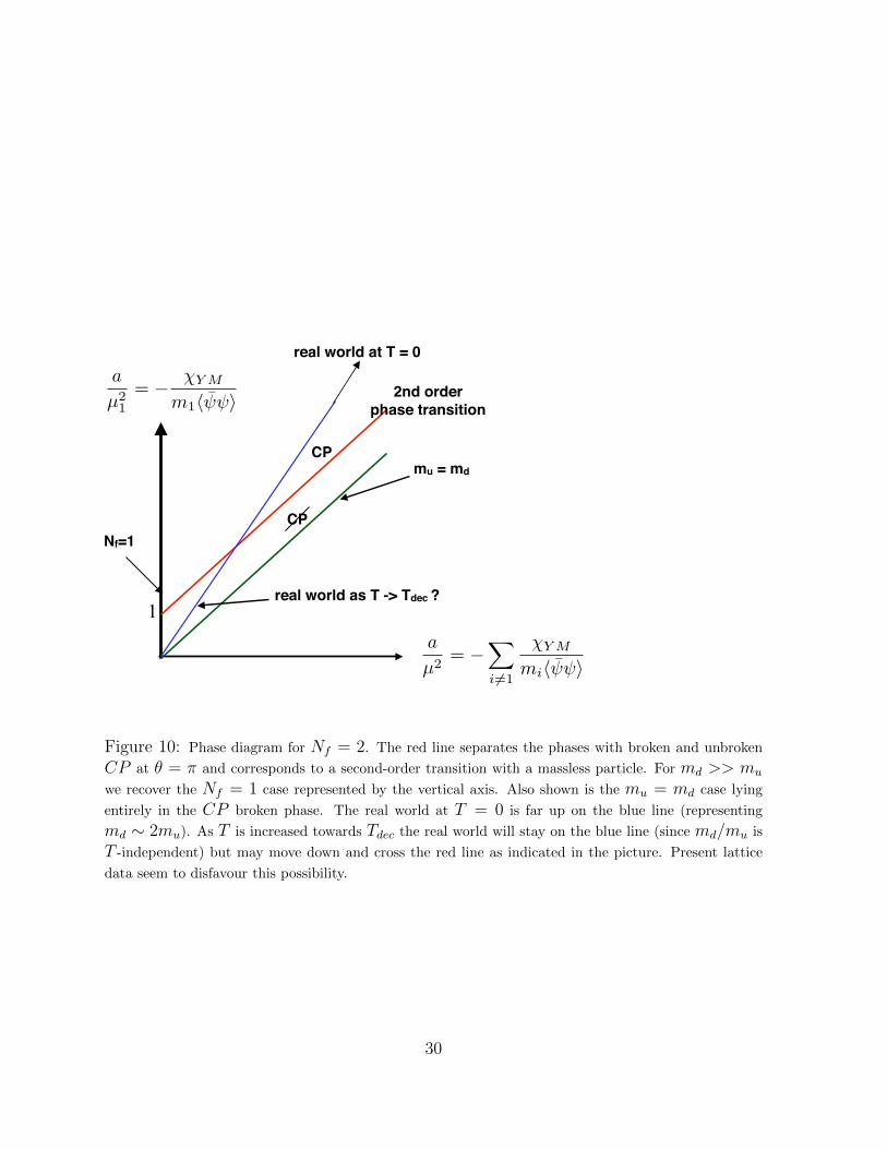
a

µ21

= � �Y M

m1h i

a

µ2= �

X

i 6=1

�Y M

mih i

1real world as T -> Tdec ?

Nf=1

mu = md

2nd order !phase transition

CP

CP

real world at T = 0

Figure 10: Phase diagram for Nf = 2. The red line separates the phases with broken and unbroken

CP at θ = π and corresponds to a second-order transition with a massless particle. For md >> mu

we recover the Nf = 1 case represented by the vertical axis. Also shown is the mu = md case lying

entirely in the CP broken phase. The real world at T = 0 is far up on the blue line (representing

md ∼ 2mu). As T is increased towards Tdec the real world will stay on the blue line (since md/mu is

T -independent) but may move down and cross the red line as indicated in the picture. Present lattice

data seem to disfavour this possibility.

30

χYM vanishes, at least in the large-N limit (dilute instantons [45, 46, 47], for instance,predict χYM ∼ e−cN) and, in that case, whether Ttop can be higher than Tch, the tempera-ture above which chiral symmetry is restored. Under reasonable assumptions, claims thatχYM should vanish above Tch were made in the past [48, 49] leaving open the possibilitythat χYM goes to zero either together or before 〈ψψ〉 does it.

Although some old lattice calculations [50] appear to point in the opposite direction(and such a possibility has its own effective Lagrangian formulation [51]), more recent sim-ulations of the pure gauge theory [52, 53] suggest the existence of a similar (or even identi-cal) value for the temperatures of deconfinement, chiral restoration and UA(1) restoration.Above the transition temperature the dilute instanton gas approximation seems to set in.Actually there is lattice evidence [54] that χYM drops rather fast above Tc for large N(and even at N = 3 a substantial decrease of χYM is visible [55, 56, 57]) and may actuallygo to zero above it for N → ∞. However, it is not clear what the ratio 〈ψψ〉planar/χYMdoes around Tc. It would thus be very interesting to plan new lattice projects dedicatedto the calculation of χYM and 〈ψψ〉 in the planar limit across the phase transition.

Recently, using the mixed CP/Center discrete anomaly matching (together with someother plausible assumptions), it was shown [27] that in YM theory the CP symmetry isspontaneously broken at θ = π and zero temperature and that the temperature Tres atwhich CP is restored is higher than the deconfinement temperature, i.e. Tres ≥ Tdec. Thisresult seems to be going in favor of the scenario advocated in [48, 49]. Breaking of CPin YM connects smoothly with CP -breaking in, say, Nf = 1 QCD at µ2/a > 1. As weincrease the temperature, if CP were restored before reaching Tdec, it would suggest that,in its QCD analog, µ2/a would go down till, at Tres, it reaches 1, which is precisely theopposite of what we were advocating, i.e. a ratio µ2/a increasing with temperature. Hencethe statement Tres ≥ Tdec is an (admittedly very mild) indication in favor of the scenarioin which the finite temperature axion potential has to be revised in a certain range oftemperature. Even if such a revision would be necessary, it remains to be seen whether itwould make any substantial difference with respect to the standard calculations [39] (seealso [58], [59]) of axionic dark matter abundance.

Acknowledgements

We thank D. Gaiotto, Z. Komargodski and N. Seiberg for informing us of theirwork [29] prior to posting it. We also thank Z. Komargodski for useful comments ona preliminary version of this manuscript as well as M. D’Elia, L. Giusti and E. Vicari fordiscussions about lattice results on Yang-Mills and quenched QCD at finite temperature.S.Y. would like to thank O. Aharony and M. Peskin for discussions. G.V. wishes to ac-knowledge an illuminating discussion with M. Shifman. The work of S.Y. is supportedin part by the I-CORE program of the Planing and Budgeting Committee (grant num-ber 1937/12), the US-Israel Binational Science Foundation (BSF), the Israel-GermanyFoundation (GIF) and the ISF Center of Excellence.

31

A Ward–Takahashi identities

In this Appendix we derive the WTIs for the anomalous UA(1) currents in QCD and checkthat the two-point amplitudes derived from the effective Lagrangian in Sect. 2 exactlysatisfy them. We start from the anomaly equation in (2.4), but written for a single flavor

∂µJµ5i = 2Q+ 2miPi ; Jµ5i = ψiγ

µγ5ψi ; Pi = iψiγ5ψi . (A.1)

Inserting the previous anomaly equation in a two-point amplitudes with another operatorO(y) we get

∂µ〈Jµ5iO(y)〉 = 〈2Q(x)O(y)〉+ δ(x0 − y0)〈[J05i, O(y)]〉+ 〈2miPi(x)O(y)〉 , (A.2)

that in Fourier space, after a partial integration, becomes

∫d4x eipx〈2Q(x)O(y)〉+ 〈[Q5i, O(y)] +

∫d4x eipx〈2miPi(x)O(y)〉

= −i∫d4x eipx〈pµJµ5i(x)O(y)〉 ; i = 1, . . . , Nf , (A.3)

where Q5i =∫d3x J0

5i(x). For O(y) = Q(y) the second term does not contribute and weget

∫d4x eipx〈2Q(x)Q(y)〉+

∫d4x eipx〈2miPi(x)Q(y)〉 = −i

∫d4x eipx〈pµJµ5i(x)Q(y)〉 , (A.4)

while, for O(y) = 2mjPj(y), the commutator gives [Q5i, Pj] = −2iψiψiδij and we get

∫d4x eipx〈2Q(x)2mjPj(y)〉+ 2iµ2

iF2π +

∫d4x eipx〈2miPi(x)2mjPj(y)〉

= −i∫d4x eipx〈pµJµ5i(x)2mjPj(y)〉 , (A.5)

having made use of the Gell-Mann–Oakes–Renner relation −2δijmi〈ψiψi〉 = δijµ2iF

2π .

One checks that the following two-point amplitudes satisfy the previous anomalousWTIs and we get

∫d4xeipx〈Q(x)Q(y)〉 = i

aF 2π

2

Nf∏

i=1

p2 − µ2i

p2 −M2i

= iaF 2

π

2

1− a

Nf∑

i=1

1

p2 − µ2i

−1

, (A.6)

∫d4xeipx〈Q(x)2miPi〉 = i

2µ2i

p2 − µ2i

aF 2π

2

Nf∏

j=1

p2 − µ2j

p2 −M2j

, (A.7)

32

∫d4xeipx〈J (i)

5µ (x)Q(y)〉 = − 2pµp2 − µ2

i

aF 2π

2

Nf∏

j=1

p2 − µ2j

p2 −M2j

, (A.8)

∫d4xeipx〈2miPi(x)2mjPj〉 =

= i2F 2

πµ4i

p2 − µ2i

δij + i4µ2

iµ2j

(p2 − µ2i )(p

2 − µ2j)

aF 2π

2

Nf∏

k=1

p2 − µ2k

p2 −M2k

, (A.9)

∫d4xeipx〈J (i)

5µ (x)2mjPj〉 =

= −2F 2πµ

2i pµ

p2 − µ2i

δij −4pµµ

2j

(p2 − µ2i )(p

2 − µ2j)

aF 2π

2

Nf∏

k=1

p2 − µ2k

p2 −M2k

. (A.10)

Furthermore, the poles at p2 = µ2i apparently present in (A.9) and (A.10) can be shown

to be absent. The only poles present are at p2 = M2i and correspond to the masses of the

physical mesons. The previous two-point amplitudes reproduce those in Sect. 2 with theidentification

miPi =⇒ Fπ√2µ2i vi . (A.11)

References

[1] R. F. Dashen, Phys. Rev. D3 (1971) 1879.

[2] J. Nuyts, Phys. Rev. Lett. 26 (1971) 1604; 27 (1971) 361.

[3] M. A. B. Beg, Phys. Rev. D4 (1971) 3810.

[4] S. Weinberg, Phys. Rev. Lett. 31 (1973) 494 and Phys. Rev. D8 (1973) 4482.

[5] G. ’t Hooft, Phys. Rev. Lett. 37 (1976) 8 and Phys. Rev. D14 (1976) 3432.

[6] R. Crewther, NATO Ad. Study Inst. Ser. B Phys. 55 (1980) 529.

[7] E. Witten, Nucl. Phys. B156 (1979) 269.

[8] G. Veneziano, Nucl. Phys. B159 (1979) 213.

[9] P. Di Vecchia, K. Fabricius, G. C. Rossi and G. Veneziano, Nucl. Phys. B192 (1981)392.

[10] L. Giusti, G. C. Rossi, M. Testa and G. Veneziano, Nucl. Phys. B628 (2002) 234.

33

[11] L. Del Debbio, L. Giusti and C. Pica, Phys. Rev. Lett. 94 (2005) 032003.

[12] M. Ce, C. Consonni, G. P. Engel and L. Giusti, Phys. Rev. D92 (2015) 074502.

[13] P. Di Vecchia, Phys. Lett. 85B (1979) 357.

[14] V. Baluni, Phys. Rev. D19 (1979) 2227.

[15] R. J. Crewther, P. Di Vecchia, G. Veneziano and E. Witten, Phys. Lett. 88B (1979)123. Erratum: [Phys. Lett. 91B (1980) 487].

[16] C. Rosenzweig, J. Schechter and C. Trahern, Phys. Rev. D21 (1980) 3388.

[17] P. Di Vecchia and G. Veneziano, Nucl. Phys. B171 (1980) 253.

[18] P. Nath and R. Arnowitt, Phys. Rev. D23 (1981) 473.

[19] E. Witten, Annals of Physics 128 (1980) 363.

[20] K. Kawarabayashi and N. Ohta, Nucl. Phys. B175 (1980) 477 and Prog. Theor. 66(1981) 1789.

[21] N. Ohta, Prog. Theor. Phys. 66 (1981) 1408.

[22] P. Di Vecchia, Acta Physica Austriaca, Suppl. XXII (1980) 341-381.

[23] P. Di Vecchia and F. Sannino, Eur. Phys. J. Plus, 129 (2014) 262.

[24] A. V. Smilga, Phys. Rev. D59 (1999) 114021.

[25] M. Creutz, Phys. Rev. Lett. 92 (2004) 201601.

[26] M. Creutz, Ann. Phys. 322 (2007) 1518, arXiv:hep-th/0609187; hep-th/0303018.

[27] D. Gaiotto, A. Kapustin, Z. Komargodski and N. Seiberg, JHEP 1705 (2017) 091.

[28] N. Seiberg, talk given at STRINGS 2017.

[29] D. Gaiotto, Z. Komargodski and N. Seiberg, arXiv:hep-th/1708.06806.

[30] G. Grilli di Cortona, E. Hardy, J. Pardo Vega and G. Villadoro, JHEP 1601 (2016)034.

[31] Z. Komargodski, A. Sharon, R. Thomgren and X. Zhou, arXiv:1705.0478 [hep-th].

[32] S.R. Sharpe, Phys. Rev. D46 (1992) 3146, hep-lat/9505020.

[33] C.W. Bernard and M.F. Golterman, Phys. Rev.D46 (1992) 853, hep-lat/9204007.

[34] L. Giusti, Nucl. Phys. Proc. Suppl. 119 (2003) 149, hep-lat/0211009.

34

[35] S. Weinberg, Phys. Rev. Lett. 40 (1978) 223.

[36] F. Wilczek, Phys. Rev. Lett 40 (1978) 279.

[37] R. Peccei and H. Quinn, Phys. Rev. Lett. 38 (1977) 1440 and Phys. Rev. D16(1977)1791.

[38] W. A. Bardeen and H. H. Tye, Phys. Lett. 74B (1978) 229.

[39] J. Preskill, M. B. Wise and F. Wilczek, Phys. Lett. 120B (1983) 127.

[40] E. Berkowitz, M. I. Buchoff and E. Rinaldi, Phys. Rev. D92 (2015) 034507.

[41] S. Borsanyi et al., Phys. Lett. 752B (2016) 175.

[42] C. Bonati, M. D’Elia, H. Panagopoulos and E. Vicari, Phys. Rev. Lett. 110, no. 25,252003 (2013).

[43] P. Chen et al., In *Vancouver 1998, High energy physics, vol. 2* 1802-1808 [hep-lat/9812011].

[44] R. G. Edwards, U. M. Heller, J. E. Kiskis and R. Narayanan, Phys. Rev. D 61,074504 (2000).

[45] D. J. Gross, R. D. Pisarski and L. G. Yaffe, Rev. Mod. Phys. 53 (1981) 43.

[46] T. Schafer and E. V. Shuryak, Rev. Mod. Phys. 70 (1998) 323.

[47] A. Ringwald and F. Schrempp, Phys. Lett. B 459 (1999) 249:

[48] G. Veneziano, Phys. Lett. 95B (1980) 90.

[49] T. D. Cohen, Phys. Rev. D 54 (1996) R1867.

[50] A. Di Giacomo, E. Meggiolaro and H. Panagopoulos, Phys. Lett. B 277 (1992) 491.

[51] E. Meggiolaro, Z. Phys. C 62 (1994) 669 and Z. Phys. C 62 (1994) 679.

[52] B. Alles, M. D’Elia and A. Di Giacomo, Nucl. Phys. B 494 (1997) 281, Erratum:[Nucl. Phys. B 679 (2004) 397].

[53] L. Del Debbio, H. Panagopoulos and E. Vicari, JHEP 0409 (2004) 028.

[54] B. Lucini, M. Teper and U. Wenger, Nucl. Phys. B 715 (2005) 461.

[55] C. Gattringer, R. Hoffmann and S. Schaefer, Phys. Lett. B 535 (2002) 358.

[56] V. G. Bornyakov, E.-M. Ilgenfritz, B. V. Martemyanov, V. K. Mitrjushkin andM. Mller-Preussker, Phys. Rev. D 87 (2013) no.11, 114508.

35

[57] G. Y. Xiong, J. B. Zhang, Y. Chen, C. Liu, Y. B. Liu and J. P. Ma, Phys. Lett. B752 (2016) 34.

[58] L. F. Abbott and P. Sikivie, Phys. Lett. 120B (1983) 133.

[59] M. Dine and W. Fischler, Phys. Lett. 120B (1983) 137.

36