SPM-BP: Sped-up PatchMatch Belief Propagation for Continuous MRFs

Yu Li, Dongbo Min, Michael S. Brown, Minh N. Do, Jiangbo Lu

2/37

Discrete Pixel-Labeling Optimization on MRF

• Many computer vision tasks can be formulated as a pixel-labeling problem on Markov Random Field (MRF)

𝑝: pixel, 𝑁𝑝: 4 neighbors

Simple: data term + smoothness term

Effective: labeling coherence, discontinuity handling

Optimization: Graph Cut, Belief Propagation, etc

Optical flow l = (u,v)

Segmentation l={B,G}

Denoising l = intensity

Stereo l = d

3/37

Belief Propagation (BP)

Iterative process in which neighbouring nodes “talk” to each other: • Update message between

neighboring pixels

• Stop after T iterations, decide the final label by picking the smallest dis-belief

1 𝑚2,1

(𝑡)

2

5

4

3

𝑚4,2(𝑡−1)

𝑚5,2(𝑡−1)

𝑚3,2(𝑡−1)

𝐸2

2

5

4 1

3

𝑚1,2𝑇

𝑚4,2𝑇

𝑚5,2𝑇

𝑚3,2𝑇

𝐸2

Challenge:

When the label set L is huge or densely sampled, BP faces prohibitively high computational challenges.

4/37

Particle Belief Propagation (PBP)

[Ihler and McAllester, “Particle Belief Propagation,” AISTATS’09]

• Solution:

(1) only store messages for K labels (particles)

l (discrete label)

l

(2) generate new label particles with the MCMC sampling using a Gaussian proposal distribution

Challenge: MCMC sampling is still inefficient and slow for continuous label spaces (e.g. stereo with slanted surfaces).

5/37

Patch Match Belief Propagation (PMBP)

2

5

4 1

3

[Besse et al, “PMBP: PatchMatch Belief Propagation for Correspondence Field Estimation,” IJCV 2014]

• Solution:

Use Patch Match[Barnes et al. Siggraph’09]’s sampling algorithm – augment PBP with label samples from the neighbours as proposals

• Orders of magnitude faster than PBP

6/37

• Effectively handles large label spaces in message passing

• Successfully applied to stereo with slanted surface modeling [Bleyer et al., BMVC’11]

Label: 3D plane normal 𝑙 = (𝑎𝑝, 𝑏𝑝, 𝑐𝑝)

Patch Match Belief Propagation (PMBP)

Left image Disparity map 3D reconstruction

• Also successfully applied to optical flow [Hornáček et al., ECCV’14]

Disparity map 3D reconstruction

𝑙 = 𝑑 (𝑖𝑛𝑡𝑒𝑔𝑒𝑟) 𝑙 = (𝑎𝑝, 𝑏𝑝, 𝑐𝑝)

Image courtesy of [Bleyer et al., BMVC’11]

7/37

Problem of PMBP

• However, it suffers from a heavy computational load on the data cost computation

• Many works strongly suggest to gather stronger

evidence from a local window for the data term

Left view Right view Weight Raw matching cost

lp

8/37

Optical Flow

Erro

r

w

Stereo

Erro

r

w

Data term is important!

• Better results with larger window sizes (2w+1)^2, but more computational cost!

w = 0

w = 4

w = 20

w = 0

w = 4

w = 20

9/37

Aggregated data cost computation

• Cross/joint/bilateral filtering principles

• Local discrete labeling approaches have often used efficient O(1)-time edge-aware filtering (EAF) methods [Rhemann et al., CVPR’11].

• O(1)-time: No dependency on window size used in EAF

Guided Filter [He et al. ECCV 2010]

Cross-based Local Multipoint Filtering (CLMF) [Lu et al. CVPR 2012]

10/37

Why does PMBP NOT use O(1) time EAF?

• Particle sampling and data cost computation are performed independently for each pixel

Incompatible with EAF, essentially exploiting redundancy

• Observation Labeling is often spatially smooth away from edges. This allows for shared label proposal and data cost computation for spatially neighboring pixels.

• Our solution A superpixel based particle sampling belief propagation method, leveraging efficient filter-based cost aggregation

Sped-up Patch Match Belief Propagation (SPM-BP)

11/37

Sped-up Patch Match Belief Propagation

• Two-Layer Graph Structures in SPM-BP

• Scan Superpixels and Perform : oNeighbourhood Propagation

oRandom Search

1. Shared particle generation 2. Shared data cost computation

1. Message passing 2. Particle selection

12/37

Related works

Pixel based MRF

Local methods [Rhemann et al., CVPR’11] [Lu et al., CVPR’13]

Only rely on data term

Superpixel based MRF [Kappes et al., IJCV’15] [Güney & Geiger, CVPR’15]

Superpixel-based MRF: each superpixel is a node in the graph and all pixels of the superpixel are constrained to have the same label.

Our two-layer graph: superpixel are employed only for particle generation and data cost computation, the labeling is performed for each pixel independently.

Superpixels as graph nodes Image courtesy of [Kappes et al., IJCV’15]

13/37

Comparison of existing labeling optimizers

Local labeling approaches Data cost computation

w/o EAF: O(|W|) w/ EAF: O(1)

Label space

handling

w/o PatchMatch: O(|L|)

Adaptive Weighting [PAMI’06]

Cost Filtering [CVPR’11]

w/ PatchMatch: O(log|L|)

PM Stereo [BMVC’11]

PMF [CVPR’13]

Global labeling approaches Data cost computation

w/o EAF: O(|W|) w/ EAF: O(1)

Label space

handling

w/o PatchMatch: O(|L|)

BP [PAMI’06]

Fully-connected CRFs [NIPS’11]

w/ PatchMatch: O(log|L|)

PMBP [IJCV’14]

SPM-BP [This paper] ?

14/37

Comparison of existing labeling optimizers

Local labeling approaches Data cost computation

w/o EAF: O(|W|) w/ EAF: O(1)

Label space

handling

w/o PatchMatch: O(|L|)

Adaptive Weighting [PAMI’06]

Cost Filtering [CVPR’11]

w/ PatchMatch: O(log|L|)

PM Stereo [BMVC’11]

PMF [CVPR’13]

Global labeling approaches Data cost computation

w/o EAF: O(|W|) w/ EAF: O(1)

Label space

handling

w/o PatchMatch: O(|L|)

BP [PAMI’06]

Fully-connected CRFs [NIPS’11]

w/ PatchMatch: O(log|L|)

PMBP [IJCV’14]

SPM-BP [This paper]

15/37

SPM-BP: Neighbourhood Propagation

Step 1. Particle propagation

Step 2. Data cost computation

Step 3. Message update

l

K=3

1-1) Randomly select one pixel from each neighbouring superpixel 1-2) Add the particles at these pixels into the proposal set

Label space

16/37

SPM-BP: Neighbourhood Propagation

Step 1. Particle propagation

Step 2. Data cost computation

Step 3. Message update

l

K=3

1-1) Randomly select one pixel from each neighbouring superpixel 1-2) Add the particles at these pixels into the proposal set

17/37

SPM-BP: Neighbourhood Propagation

Step 1. Particle propagation

Step 2. Data cost computation

Step 3. Message update

p Ep(l)

l

l = l1 l1

2-1) Compute the raw matching data cost of these labels in a slightly enlarged region 2-2) Compute the aggregated data cost for each label by performing EAF on the raw matching cost

18/37

SPM-BP: Neighbourhood Propagation

Step 1. Particle propagation

Step 2. Data cost computation

Step 3. Message update

p Ep(l)

l

l = l1

l = l2

l = l15

l1

2-1) Compute the raw matching data cost of these labels in a slightly enlarged region 2-2) Compute the aggregated data cost for each label by performing EAF on the raw matching cost

19/37

SPM-BP: Neighbourhood Propagation

Step 1. Particle propagation

Step 2. Data cost computation

Step 3. Message update

l

3-1) Perform message passing for pixels within the superpixel.

20/37

SPM-BP: Neighbourhood Propagation

Step 1. Particle propagation

Step 2. Data cost computation

Step 3. Message update

3-1) Perform message passing for pixels within the superpixel. 3-2) Keep K particles with the smallest disbeliefs at each pixel.

l

keep K particles

top K particles

21/37

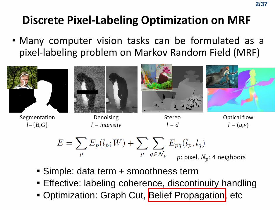
SPM-BP: Random Search

Step 1. Particle propagation

Step 2. Data cost computation

Step 3. Message update

l

1-1) Randomly select one pixel in the visiting superpixel

22/37

SPM-BP: Random Search

Step 1. Particle propagation

Step 2. Data cost computation

Step 3. Message update

l

1-1) Randomly select one pixel in the visiting superpixel 1-2) Generate new proposals around the sampled particles

23/37

SPM-BP: Random Search

Step 1. Particle propagation

Step 2. Data cost computation

Step 3. Message update

p Ep(l)

l = l1

l = l2

l = l15

l

2-1) Compute the raw matching data cost of these labels in a slightly enlarged region 2-2) Compute the aggregated data cost for each label by performing EAF on the raw matching cost

24/37

SPM-BP: Random Search

Step 1. Particle propagation

Step 2. Data cost computation

Step 3. Message update

3-1) Perform message passing for pixels within the superpixel. 3-2) Keep K particles with the smallest disbeliefs at each pixel.

l

keep K particles

25/37

SPM-BP: Recap

Data cost computation

using EAF

Message passing at pixel

level

Iterate

Superpixel based

particle generation

Random Initialization

Final labels

26/37

Complexity Comparison

|W| – local window size (e.g. 31x31 for stereo) K – number of particles used (small constant) N – number of pixels L – label space size (e.g. over 10 million for flow)

*PMF stores only one best particle (K = 1) per pixel node, thus requiring more iterations than the other two methods.

27/37

Example Applications

• Stereo with slanted surface supports

• label: 3D plane normal 𝑙𝑝 = (𝑎𝑝, 𝑏𝑝, 𝑐𝑝)

• Matching features: color + gradient

• Smoothness term: deviation between two local planes

• Cross checking + post processing for occlusion

• Large-displacement optical flow

• label: 2D displacement vector 𝑙𝑝 = (𝑢, 𝑣)

• Matching features: color + Census transform

• Smoothness term: truncated L2 distance

• Cross checking + post processing for occlusion

28/37

#iteration = 5, K = 3

K = 3

Convergence

29/37

Convergence

K = 3

30/37

Stereo results

SPM-BP (ours)

30 sec. PMBP

3100 sec.

Stereo input

PMF

20 sec.

Much faster than PMBP, and much better than PMF for textureless regions

31/37

Stereo results

SPM-BP (ours) PMBP

Stereo input

PMF SPM-BP (ours)

30 sec. PMBP

3100 sec.

PMF

20 sec.

32/37

Optical flow results

Optical flow input PMBP

2103 sec.

SPM-BP (ours)

42 sec.

PMF

27 sec.

Much faster than PMBP, and much better than PMF for textureless regions

33/37

Optical flow results

34/37

Performance Evaluation

Remarks • A simple formulation, without

needing complex energy terms

nor a separate initialization

• Achieved top-tier performance,

even when compared to task-

specific techniques

• Applied on the full pixel grid,

avoiding coarse-to-fine steps

Middlebury Stereo Performance (Tsukuba/Venus/Teddy/Cones )

Optical Flow Performance on MPI Sintel Benchmark (captured on 16/04/2015)

Middlebury Stereo 2006 Performance

35/37

Conclusion

• SPM-BP is simple, effective and efficient

• Takes the best computational advantages of efficient edge-aware cost filtering

and superpixel-based particle-sampling for message passing

• Offers itself as a general and efficient global optimizer for

continuous MRFs

• Future work

Robust dense correspondences for cross-scene matching

Dealing with high-order terms in MRF

Code available online: http://publish.illinois.edu/visual-modeling-and-

analytics/efficient-inference-for-continuous-mrfs/