Embed Size (px)
Citation preview
JSS Journal of Statistical SoftwareApril 2012, Volume 47, Issue 1. http://www.jstatsoft.org/
splm: Spatial Panel Data Models in R
Giovanni MilloGenerali SpA
Gianfranco PirasWest Virginia University
Abstract
splm is an R package for the estimation and testing of various spatial panel data spec-ifications. We consider the implementation of both maximum likelihood and generalizedmoments estimators in the context of fixed as well as random effects spatial panel datamodels. This paper is a general description of splm and all functionalities are illustratedusing a well-known example taken from Munnell (1990) with productivity data on 48 USstates observed over 17 years. We perform comparisons with other available software;and, when this is not possible, Monte Carlo results support our original implementation.
Keywords: spatial panel, maximum likelihood, GM, LM tests, spatial Hausman test, R.
1. Introduction
The analysis of spatial panel data is a field of econometrics that is experiencing increasedmethodological progress. Recent contributions include, among others: Anselin, Le Gallo, andJayet (2008), Kapoor, Kelejian, and Prucha (2007), Baltagi, Song, Jung, and Koh (2007b),Baltagi, Song, and Koh (2003), Baltagi and Liu (2008), Baltagi, Egger, and Pfaffermayr(2007a), Baltagi, Egger, and Pfaffermayr (2009), Debarsy and Ertur (2010), Elhorst (2003),Elhorst and Freret (2009), Elhorst (2008), Elhorst (2009), Elhorst (2010), Elhorst, Piras, andArbia (2010), Lee and Yu (2010a), Lee and Yu (2010c), Lee and Yu (2010d), Lee and Yu(2010b), Mutl (2006), Mutl and Pfaffermayr (2011), Pesaran and Tosetti (2011), Yu and Lee(2010), Yu, de Jong, and Lee (2008). Empirical applications are hindered by the lack of readilyavailable software. Although there are packages to estimate cross-sectional spatial models inR (R Development Core Team 2012, see e.g., Bivand 2001, 2002, 2006; Bivand and Gebhardt2000; Bivand and Portnov 2004; Piras 2010), MATLAB (The MathWorks, Inc. 2010, see e.g.,LeSage 1999; LeSage and Pace 2009) and Stata (StataCorp. 2007, see e.g., Drukker, Peng,Prucha, and Raciborski 2012, 2011a; Drukker, Prucha, and Raciborski 2011c,b), proceduresfor estimating spatial panel data models are sparse. Notable exceptions include the MATLABfunctions available from Elhorst (2011) and the Stata code supplementing Kapoor et al. (2007).
2 splm: Spatial Panel Data Models in R
The R package splm – available from the Comprehensive R Archive Network at http://CRAN.R-project.org/package=splm – fills this gap by providing a comprehensive and consistenttool for the estimation of various spatial panel data models. The R environment is ideal forits development because of the vast infrastructure already in place for analyzing spatial data.
The panel literature has recently considered panel regression models with spatially auto-correlated disturbances, both in the context of fixed (FE) as well as random effects (RE)specifications. In an error components setting, Baltagi et al. (2003) introduce a model (alsoconsidered in Anselin 1988) where the idiosyncratic errors are spatially autocorrelated, whilethe individual effects are not. The variance matrix of such a model is complicated and theinverse computationally demanding. Kapoor et al. (2007) consider a model where spatial cor-relation in both the individual and error components share the same spatial parameter; and,therefore, the expression of the variance matrix is simpler and its inverse computationally eas-ier. splm takes into consideration both specifications and several methods for the estimationof the regression coefficients.
The present paper describes the maximum likelihood implementation of both models (i.e.,with individual effects that are/are not spatially autocorrelated). We consider fixed as well asrandom effects models in the context of a general spatial Cliff-Ord type model that includesa spatially lagged dependent variable and a spatially autocorrelated error term.
Additionally, splm features generalized moments estimators of a Cliff-Ord type model whereindividual effects are spatially autocorrelated. Again, random as well as fixed effects modelsare implemented. When other implementations were available, the estimates obtained by ourimplementation were tested against results available from other software. As an example, themaximum likelihood estimation of the fixed effects and random effects models were testedagainst the MATLAB routines made available by Elhorst (2011). For all other estimationprocedures we performed Monte Carlo simulations to verify the properties of our estimator.Results are presented in Section 8.
Among other testing procedures, we also implement the joint, marginal and conditional specifi-cation (zero-restriction) Lagrange multiplier tests for individual effects and spatial correlationintroduced by Baltagi et al. (2003).
Section 2 describes the data structure. In Section 3 we discuss the definition of classes andmethods. The description of a general spatial panel regression model follows in Section 4along with the treatment of two different specifications for the innovations of the model.Section 5 is devoted to the maximum likelihood (ML) implementation. In particular, Sec-tion 5.1 discusses and illustrates spatial random effects (RE) models, while Section 5.2 dealswith the estimation of fixed effects (FE) models. Section 6 describes the implementationof the generalized moments estimators. As before, spatial RE models are discussed first inSection 6.1. Section 6.2 present the estimation theory and the generalized moments (GM)implementation of fixed effects models. Section 7 describes the implementation of varioustesting procedures and Section 8 discusses the numerical checks. Conclusions and indicationsfor future developments conclude the paper.
2. Data structures
Panel data refer to a cross section of observations (individuals, groups, countries, regions)repeated over several time periods. When the number of cross sectional observations is con-

Journal of Statistical Software 3
stant across time periods the panel is said to be balanced. The present paper only focuseson such balanced panels. In a spatial panel setting, the observations are associated with aparticular position in space. Data can be observed either at point locations (e.g., housingdata) or aggregated over regular or irregular areas (e.g., countries, regions, states, counties).The structure of the interactions between each pair of spatial units is represented by meansof a spatial weights matrix.
The spatial weights matrix W is a N ×N positive matrix.1 Observations appear both in rowsand columns. Hence, the non-zero elements of the matrix indicate whether two locationsare neighbors. As a consequence, the element wij indicates the intensity of the relationshipbetween cross sectional units i and j. By convention, the diagonal elements wii are all setto zero to exclude self-neighbors. The weights matrix is generally used in row standardizedform.
A possible source of confusion when developing ad-hoc routines stems from the differentnotation that characterizes spatial panel data models compared to traditional panel datamodels. On one hand, panel data are generally ordered first by cross-section and then bytime period (i.e., with time being the “fast” index). On the other hand, spatial panel data arestacked first by time period and then by cross-section. In splm, this is treated transparentlyfor the user. The internal ordering of the estimation functions is usually (but not always)the spatial panel data one. Nonetheless, data can be supplied according to the conventionsimplemented in the plm package for panel data econometrics (Croissant and Millo 2008).Three possibilities are available:
a data.frame whose first two variables are the individual and time indexes. The index
argument should be left to the default value (i.e., NULL)
a data.frame and a character vector indicating the indexes variables
an object of the class pdata.frame
pdata.frames are special objects created to deal with panel data. They are part of a generalinfrastructure made available in plm and meant to handle (serial) lag and difference opera-tions. The methods available in splm are geared towards static panels; nonetheless, definingdata as a pdata.frame might simplify the calculation of (time) lags of the regressors.2
The spatial weights matrix W can be a matrix object (with the estimators performing aminimal check for dimension compatibility) or a listw object from the class defined in spdep(Bivand 2011).3 The class is an efficient format and has the advantage of being well establishedin the R environment. Functionalities for switching between the two formats are available asfunctions listw2mat and mat2listw from the spdep package.
1The spatial weights matrix may or may not be symmetric. When it is standardized, it is generally notsymmetric. splm can deal with all types of matrices. However, some of the methods for the calculation of theJacobian are only used with symmetric weights. We will elaborate more on this later.
2It should be made clear that the inclusion of time lags would potentially lead to incorrect results for adynamic model estimated with the procedures currently available. However, future improvements may includedynamic panel data models in which case pdata.frame objects would be extremely useful.
3Some of the functions internally transform the object of class listw into a sparse Matrix making use ofcode from the Matrix package (Bates and Machler 2012).
4 splm: Spatial Panel Data Models in R
3. Classes and methods for spatial panel models
The two main goals of splm are estimation and testing of spatial panel data models. On theone hand, the information provided in the output of the test procedures is similar to an objectof class htest; and, hence, produces a similar output report. On the other hand, spatial panelmodels require different structures and methods from the classes available in plm. By andlarge, this is because spatial panel models involve the estimation of extra coefficients (e.g., thecoefficient for the spatial lag term in the fixed effects spatial lag model or the error correlationcoefficient and the variance components in the random effects specifications).
The new class splm inherits the general structure of lm objects. The splm object is a list
of various elements including: the estimated coefficients, the vector of residuals andfitted.values, the most recent call and a model element containing the data employed inthe estimation. As it is common for most models that are estimated by maximum likelihood,splm also comprises a logLik component with the value of the log-likelihood at the parameteroptimum. This can be easily extracted and reused for testing or model selection purposes.
Some elements from lm objects have been excluded though. These omissions are partly due tothe nature of the estimation process (which does not use, for instance, the“qr”decomposition).Specific elements have been added to accommodate for spatial and covariance parameters.In addition to the usual vcov element giving the coefficients’ variance covariance matrix,the element vcov.errcomp contains the covariance matrix of the estimated error covariancecoefficients.
A new class is defined for the summaries of splm objects. Consistent with lm and plm objects,the method provides diagnostic tables for the elements of splm objects. print methods arealso available with a minimal description of the model object (including call, coefficients andcovariance parameters). Additionally, extractor methods have been defined for a few relevantelements of model objects. Along with the standard coef, residuals, and vcov, extractormethods are provided for the covariance matrices of the estimated spatial autoregressivecoefficient and covariance components.
The availability of these extractors is consistent with the general modeling framework of theR project and favors the interoperability of splm objects with generic diagnostics based onWald tests. In particular we refer to the functions waldtest (for joint zero-restrictions) inlmtest (Zeileis and Hothorn 2002) and linearHypothesis (for generic linear restrictions) incar (Fox and Weisberg 2010).
Finally, an extractor method for fixed effects and a summary method for displaying them arealso available.
Throughout the paper, all functionalities are illustrated using the well-known Munnell (1990)data set on public capital productivity in 48 US states observed over 17 years (available in Rin the Ecdat package, Croissant 2011). A binary contiguity spatial weights matrix for the USstates is included in the package.
R> data("Produc", package = "Ecdat")
R> data("usaww")
Munnell (1990) specifies a Cobb-Douglas production function that relates the gross socialproduct (gsp) of a given state to the input of public capital (pcap), private capital (pc), labor(emp) and state unemployment rate (unemp) added to capture business cycle effects. Themodel formula is defined once and includes a constant term:

Journal of Statistical Software 5
R> fm <- log(gsp) ~ log(pcap) + log(pc) + log(emp) + unemp
We also transform the weights matrix into a listw object using infrastructure from the spdeppackage:
R> library("spdep")
R> usalw <- mat2listw(usaww)
4. Spatial panel data models
Spatial panel data models capture spatial interactions across spatial units and over time.There is an extensive literature on both static as well as dynamic models.4 We start from ageneral static panel model that includes a spatial lag of the dependent variable and spatialautoregressive disturbances:
y = λ(IT ⊗WN )y +Xβ + u (1)
where y is an NT ×1 vector of observations on the dependent variable, X is a NT ×k matrixof observations on the non-stochastic exogenous regressors, IT an identity matrix of dimensionT , WN is the N ×N spatial weights matrix of known constants whose diagonal elements areset to zero, and λ the corresponding spatial parameter. The disturbance vector is the sum oftwo terms
u = (ιT ⊗ IN )µ+ ε (2)
where ιT is a T × 1 vector of ones, IN an N × N identity matrix, µ is a vector of time-invariant individual specific effects (not spatially autocorrelated), and ε a vector of spatiallyautocorrelated innovations that follow a spatial autoregressive process of the form
ε = ρ(IT ⊗WN )ε+ ν (3)
with ρ (|ρ| < 1) as the spatial autoregressive parameter, WN the spatial weights matrix,νit ∼ IID(0, σ2ν) and εit ∼ IID(0, σ2ε).
5
As in the classical panel data literature, the individual effects can be treated as fixed orrandom. In a random effects model, one is implicitly assuming that the unobserved individualeffects are uncorrelated with the other explanatory variables in the model. In this case,µi ∼ IID(0, σ2µ), and the error term can be rewritten as:
ε = (IT ⊗B−1N )ν (4)
where BN = (IN − ρWN ). As a consequence, the error term becomes
u = (ιT ⊗ IN )µ+ (IT ⊗B−1N )ν (5)
4In our discussion, as well as in our implementation, we concentrate on static models only and leave thedynamic case as a possible extension for future research.
5Note that the spatial weights matrices in the regression equation and the error term can differ in many ofour implementations. However, in our discussion of the models they are assumed to be the same for simplicity.It is also assumed that IN − ρWN is non-singular where IN is an identity matrix of dimension N .
6 splm: Spatial Panel Data Models in R
and the variance-covariance matrix for ε is
Ωu = σ2µ(ιT ι>T ⊗ IN ) + σ2ν [IT ⊗ (B>NBN )−1] (6)
In deriving several Lagrange multiplier (LM) tests, Baltagi et al. (2003) consider a paneldata regression model that is a special case of the model presented above in that it does notinclude a spatial lag of the dependent variable. Elhorst (2003, 2009) defines a taxonomy forspatial panel data models both under the fixed and the random effects assumptions. Followingthe typical distinction made in cross-sectional models, Elhorst (2003, 2009) defines the fixedas well as the random effects panel data versions of the spatial error and spatial lag models.However, he does not consider a model including both the spatial lag of the dependent variableand a spatially autocorrelated error term. Therefore, the models reviewed in Elhorst (2003,2009) can also be seen as a special case of this more general specification.
A second specification for the disturbances is considered in Kapoor et al. (2007). They as-sume that spatial correlation applies to both the individual effects and the remainder errorcomponents. Although the two data generating processes look similar, they do imply differentspatial spillover mechanisms governed by a different structure of the implied variance covari-ance matrix. In this case, the disturbance term follows a first order spatial autoregressiveprocess of the form:
u = ρ(IT ⊗WN )u+ ε (7)
where WN is the spatial weights matrix and ρ the corresponding spatial autoregressive param-eter. To further allow for the innovations to be correlated over time, the innovations vectorin Equation 7 follows an error component structure
ε = (ιT ⊗ IN )µ+ ν (8)
where µ is the vector of cross-sectional specific effects, ν a vector of innovations that varyboth over cross-sectional units and time periods, ιT is a vector of ones and IN an N × Nidentity matrix. In deriving a Hausman test for a Cliff and Ord spatial panel data model,Mutl and Pfaffermayr (2011) consider the model presented above and discuss instrumentalvariables estimation under both the fixed and the random effects specifications. They extendthe work of Kapoor et al. (2007) who did not include a spatially lagged dependent variablein the regression equation. Under the random effects assumption that the individual effectsare independent of the model regressors, one can rewrite Equation 7 as
u = [IT ⊗ (IN − ρWN )−1]ε (9)
It follows that the variance-covariance matrix of u is
Ωu = [IT ⊗ (IN − ρWN )−1]Ωε[IT ⊗ (IN − ρW>N )−1] (10)
where Ωε = σ2νQ0 + σ21Q1, with σ21 = σ2ν + Tσ2µ, Q0 =(IT − JT
T
)⊗ IN , Q1 = JT
T ⊗ IN and
JT = ιT ι>T , is the typical variance-covariance matrix of a one-way error component model
adapted to the different ordering of the data.
As it should be clear from the above discussion, these two panel models differ in terms oftheir variance matrices. The variance matrix in Equation 6 is more complicated than the onein Equation 10, and, therefore, its inverse is more difficult to calculate. In the present paper,
Journal of Statistical Software 7
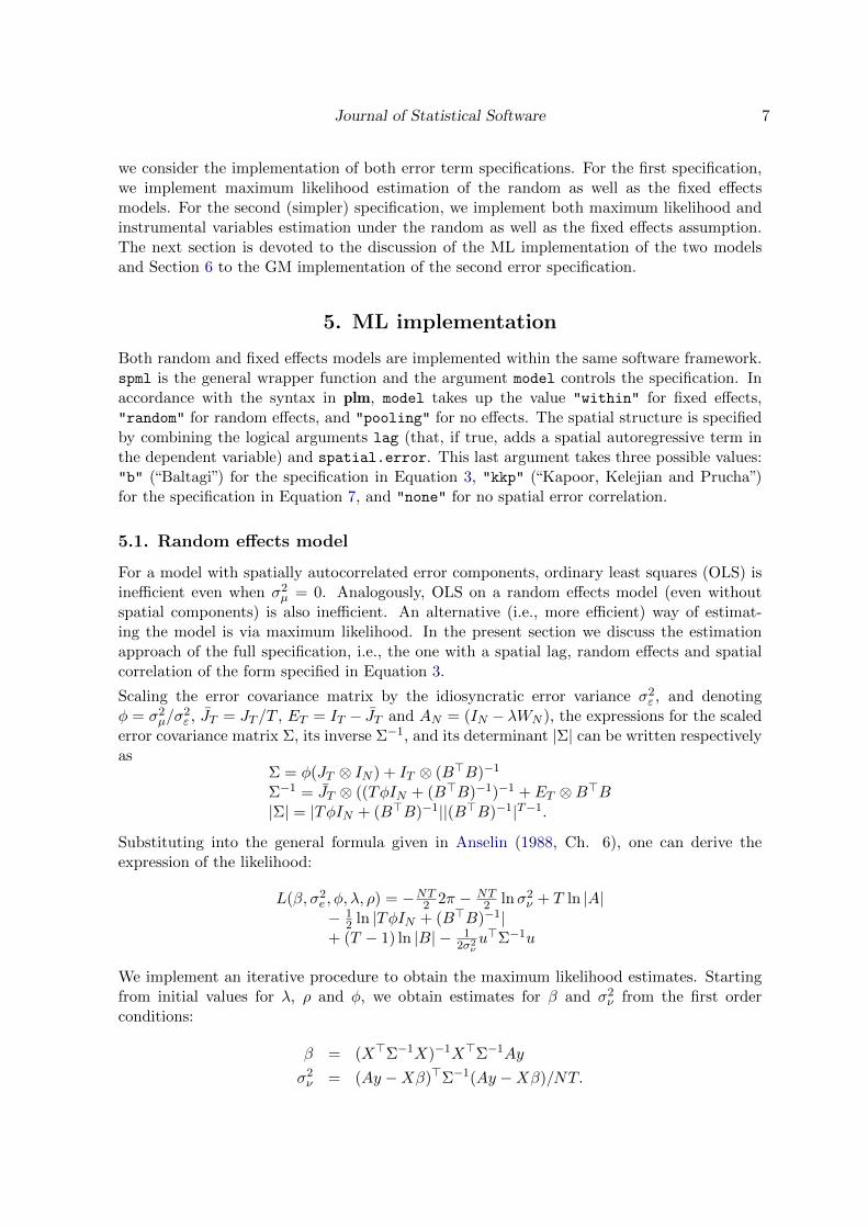
we consider the implementation of both error term specifications. For the first specification,we implement maximum likelihood estimation of the random as well as the fixed effectsmodels. For the second (simpler) specification, we implement both maximum likelihood andinstrumental variables estimation under the random as well as the fixed effects assumption.The next section is devoted to the discussion of the ML implementation of the two modelsand Section 6 to the GM implementation of the second error specification.
5. ML implementation
Both random and fixed effects models are implemented within the same software framework.spml is the general wrapper function and the argument model controls the specification. Inaccordance with the syntax in plm, model takes up the value "within" for fixed effects,"random" for random effects, and "pooling" for no effects. The spatial structure is specifiedby combining the logical arguments lag (that, if true, adds a spatial autoregressive term inthe dependent variable) and spatial.error. This last argument takes three possible values:"b" (“Baltagi”) for the specification in Equation 3, "kkp" (“Kapoor, Kelejian and Prucha”)for the specification in Equation 7, and "none" for no spatial error correlation.
5.1. Random effects model
For a model with spatially autocorrelated error components, ordinary least squares (OLS) isinefficient even when σ2µ = 0. Analogously, OLS on a random effects model (even withoutspatial components) is also inefficient. An alternative (i.e., more efficient) way of estimat-ing the model is via maximum likelihood. In the present section we discuss the estimationapproach of the full specification, i.e., the one with a spatial lag, random effects and spatialcorrelation of the form specified in Equation 3.
Scaling the error covariance matrix by the idiosyncratic error variance σ2ε , and denotingφ = σ2µ/σ
2ε , JT = JT /T , ET = IT − JT and AN = (IN − λWN ), the expressions for the scaled
error covariance matrix Σ, its inverse Σ−1, and its determinant |Σ| can be written respectivelyas
Σ = φ(JT ⊗ IN ) + IT ⊗ (B>B)−1
Σ−1 = JT ⊗ ((TφIN + (B>B)−1)−1 + ET ⊗B>B|Σ| = |TφIN + (B>B)−1||(B>B)−1|T−1.
Substituting into the general formula given in Anselin (1988, Ch. 6), one can derive theexpression of the likelihood:
L(β, σ2e , φ, λ, ρ) = −NT2 2π − NT
2 lnσ2ν + T ln |A|− 1
2 ln |TφIN + (B>B)−1|+ (T − 1) ln |B| − 1
2σ2νu>Σ−1u
We implement an iterative procedure to obtain the maximum likelihood estimates. Startingfrom initial values for λ, ρ and φ, we obtain estimates for β and σ2ν from the first orderconditions:
β = (X>Σ−1X)−1X>Σ−1Ay
σ2ν = (Ay −Xβ)>Σ−1(Ay −Xβ)/NT.
8 splm: Spatial Panel Data Models in R
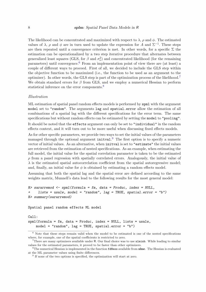
The likelihood can be concentrated and maximized with respect to λ, ρ and φ. The estimatedvalues of λ, ρ and φ are in turn used to update the expression for A and Σ−1. These stepsare then repeated until a convergence criterion is met. In other words, for a specific Σ theestimation can be operationalized by a two step iterative procedure that alternates betweengeneralized least squares (GLS, for β and σ2ν) and concentrated likelihood (for the remainingparameters) until convergence.6 From an implementation point of view there are (at least) acouple of different ways to proceed. First of all, we decided to include the GLS step withinthe objective function to be maximized (i.e., the function to be used as an argument to theoptimizer). In other words, the GLS step is part of the optimization process of the likelihood.7
We obtain standard errors for β from GLS, and we employ a numerical Hessian to performstatistical inference on the error components.8
Illustration
ML estimation of spatial panel random effects models is performed by spml with the argumentmodel set to "random". The arguments lag and spatial.error allow the estimation of allcombinations of a spatial lag with the different specifications for the error term. The samespecifications but without random effects can be estimated by setting the model to "pooling".
It should be noted that the effects argument can only be set to "individual" in the randomeffects context, and it will turn out to be more useful when discussing fixed effects models.
As for other specific parameters, we provide two ways to set the initial values of the parametersmanaged through the optional argument initval.9 The first option is to specify a numericvector of initial values. As an alternative, when initval is set to "estimate" the initial valuesare retrieved from the estimation of nested specifications. As an example, when estimating thefull model, the initial value for the spatial correlation parameter is taken to be the estimatedρ from a panel regression with spatially correlated errors. Analogously, the initial value ofλ is the estimated spatial autocorrelation coefficient from the spatial autoregressive model;and, finally, an initial value for φ is obtained by estimating a random effects model.
Assuming that both the spatial lag and the spatial error are defined according to the sameweights matrix, Munnell’s data lead to the following results for the most general model:
R> sararremod <- spml(formula = fm, data = Produc, index = NULL,
+ listw = usalw, model = "random", lag = TRUE, spatial.error = "b")
R> summary(sararremod)
Spatial panel random effects ML model
Call:
spml(formula = fm, data = Produc, index = NULL, listw = usalw,
model = "random", lag = TRUE, spatial.error = "b")
6 Note that these steps remain valid when the model to be estimated is one of the nested specificationswhere, for example, one of the spatial coefficients is restricted to zero.
7There are many optimizers available under R. Our final choice was to use nlminb. While leading to similarvalues for the estimated parameters, it proved to be faster than other optimizers.
8The numerical Hessian is implemented in the function fdHess available from nlme. The Hessian is evaluatedat the ML parameter values using finite differences.
9 If none of the two options is specified, the optimization will start at zero.
Journal of Statistical Software 9
Residuals:
Min. 1st Qu. Median Mean 3rd Qu. Max.
-0.2480 -0.0411 0.0123 0.0191 0.0726 0.4840
Error variance parameters:
Estimate Std. Error t-value Pr(>|t|)
phi 7.530808 1.743935 4.3183 1.572e-05 ***
rho 0.536835 0.034481 15.5690 < 2.2e-16 ***
Spatial autoregressive coefficient:
Estimate Std. Error t-value Pr(>|t|)
lambda 0.0018174 0.0058998 0.3081 0.758
Coefficients:
Estimate Std. Error t-value Pr(>|t|)
(Intercept) 2.3736012 0.1394745 17.0182 < 2.2e-16 ***
log(pcap) 0.0425013 0.0222146 1.9132 0.055721 .
log(pc) 0.2415077 0.0202971 11.8987 < 2.2e-16 ***
log(emp) 0.7419074 0.0244212 30.3797 < 2.2e-16 ***
unemp -0.0034560 0.0010605 -3.2589 0.001119 **
---
Signif. codes: 0 '***' 0.001 '**' 0.01 '*' 0.05 '.' 0.1 ' ' 1
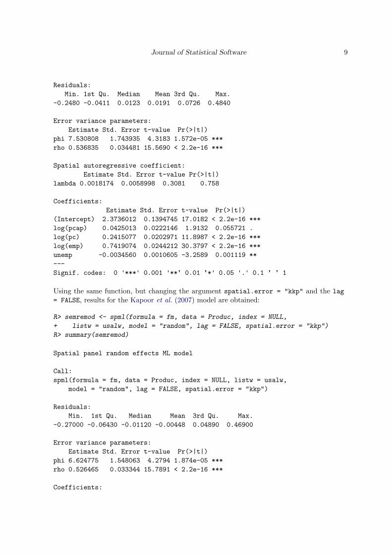
Using the same function, but changing the argument spatial.error = "kkp" and the lag
= FALSE, results for the Kapoor et al. (2007) model are obtained:
R> semremod <- spml(formula = fm, data = Produc, index = NULL,
+ listw = usalw, model = "random", lag = FALSE, spatial.error = "kkp")
R> summary(semremod)
Spatial panel random effects ML model
Call:
spml(formula = fm, data = Produc, index = NULL, listw = usalw,
model = "random", lag = FALSE, spatial.error = "kkp")
Residuals:
Min. 1st Qu. Median Mean 3rd Qu. Max.
-0.27000 -0.06430 -0.01120 -0.00448 0.04890 0.46900
Error variance parameters:
Estimate Std. Error t-value Pr(>|t|)
phi 6.624775 1.548063 4.2794 1.874e-05 ***
rho 0.526465 0.033344 15.7891 < 2.2e-16 ***
Coefficients:
10 splm: Spatial Panel Data Models in R
Estimate Std. Error t-value Pr(>|t|)
(Intercept) 2.3246707 0.1415894 16.4184 < 2.2e-16 ***
log(pcap) 0.0445475 0.0220377 2.0214 0.0432362 *
log(pc) 0.2461124 0.0211341 11.6453 < 2.2e-16 ***
log(emp) 0.7426319 0.0254663 29.1614 < 2.2e-16 ***
unemp -0.0036045 0.0010637 -3.3887 0.0007022 ***
---
Signif. codes: 0 '***' 0.001 '**' 0.01 '*' 0.05 '.' 0.1 ' ' 1
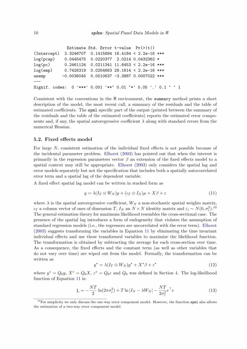
Consistent with the conventions in the R environment, the summary method prints a shortdescription of the model, the most recent call, a summary of the residuals and the table ofestimated coefficients. The spml specific part of the output (printed between the summary ofthe residuals and the table of the estimated coefficients) reports the estimated error compo-nents and, if any, the spatial autoregressive coefficient λ along with standard errors from thenumerical Hessian.
5.2. Fixed effects model
For large N, consistent estimation of the individual fixed effects is not possible because ofthe incidental parameter problem. Elhorst (2003) has pointed out that when the interest isprimarily in the regression parameters vector β an extension of the fixed effects model to aspatial context may still be appropriate. Elhorst (2003) only considers the spatial lag anderror models separately but not the specification that includes both a spatially autocorrelatederror term and a spatial lag of the dependent variable.
A fixed effect spatial lag model can be written in stacked form as
y = λ(IT ⊗WN )y + (ιT ⊗ IN )µ+Xβ + ε (11)
where λ is the spatial autoregressive coefficient, WN a non-stochastic spatial weights matrix,ιT a column vector of ones of dimension T , IN an N ×N identity matrix and εi ∼ N(0, σ2ε).
10
The general estimation theory for maximum likelihood resembles the cross-sectional case. Thepresence of the spatial lag introduces a form of endogeneity that violates the assumption ofstandard regression models (i.e., the regressors are uncorrelated with the error term). Elhorst(2003) suggests transforming the variables in Equation 11 by eliminating the time invariantindividual effects and use these transformed variables to maximize the likelihood function.The transformation is obtained by subtracting the average for each cross-section over time.As a consequence, the fixed effects and the constant term (as well as other variables thatdo not vary over time) are wiped out from the model. Formally, the transformation can bewritten as
y∗ = λ(IT ⊗WN )y∗ +X∗β + ε∗ (12)
where y∗ = Q0y, X∗ = Q0X, ε∗ = Q0ε and Q0 was defined in Section 4. The log-likelihoodfunction of Equation 11 is:
L = −NT2
ln(2πσ2ε) + T ln |IN − λWN | −NT
2σ2εe>e (13)
10For simplicity we only discuss the one-way error component model. However, the function spml also allowsthe estimation of a two-way error component model.

Journal of Statistical Software 11
where e = y− λ(IT ⊗WN )y−Xβ and ln |IN − λWN | is the Jacobian determinant.11 Elhorst(2009) suggests a concentrated likelihood approach for maximizing Equation 13. The esti-mation procedure is substantially analogous to the one employed in the cross-sectional case.After the transformation, two auxiliary regressions of y∗ and (IN ⊗WN )y∗ on X∗ are per-formed. The corresponding residuals (say e∗0 and e∗1) are combined to obtain the concentratedlikelihood:
L = C + T ln |IN − λWN | −NT
2ln[(e∗0 − λe∗1)>(e∗0 − λe∗1)] (14)
with C a constant not depending on λ. A numerical optimization procedure is needed toobtain the value of λ that maximizes Equation 14. Finally, estimates for β and σ2ε areobtained from the first order conditions of the likelihood function by replacing λ with itsestimated value from the ML. Analogous to the cross sectional model, the estimator for βcan also be seen as the generalized least square estimator of a linear regression model withdisturbance variance matrix σ2εQ0.
12 Statistical inference on the parameters of the model canbe based on the expression for the asymptotic variance covariance matrix derived in Elhorst(2009) and Elhorst and Freret (2009): AsyVar(β, λ, σ2ε) =
1σ2εX∗>X∗ 1
σ2εX∗>(IT ⊗ W )X∗β
1σ2εβ>X∗>(IT ⊗ W>W )X∗β + T tr(WW + W ′W )
Tσ2ε
tr(W ) NT2σ4ε
−1
(15)
where W = W (IN − λW )−1 and the missing elements that cannot be filled in by symmetryare zeros. The computational burden involved in the calculation of the asymptotic standarderror of the spatial parameter can be very costly for large problem dimensions (mainly becauseof the inverse of the N × N matrix involved in the computation). The block of the coeffi-cient covariance matrix relative to the parameter vector β does not present any particularcomputational difficulties. Fixed effects can be recovered by
µi =1
T
T∑t=1
(yit − λN∑j=1
wijyjt − xitβ) (16)
Averaging across all observations one can also recover the intercept under the restriction thatthe individual effects sum to zero (see also Baltagi 2008, p. 13).
A fixed effects spatial error model can be written as
y = (ιT ⊗ IN )µ+Xβ + u
u = ρ(IT ⊗WN )u+ ε (17)
11 Sometimes the likelihood is expressed in terms of the log Jacobian∑i ln(1 − λωi) where ωi are the
eigenvalues of the spatial weights matrix. The default method to compute the Jacobian is based on theeigenvalues decomposition using the functions eigenw. In line with the changes and improvements recentlymade in spdep (Bivand 2010), other methods are available, including the use of sparse matrices, and theChebyshev and Monte Carlo approximations (LeSage and Pace 2009).
12 Anselin et al. (2008) point out that various aspects of the fixed effects spatial lag model deserve furtherinvestigation. The main issue relates to the properties of Q0. By definition Q0 is singular and therefore |Q0|does not exist. While this is not a problem in the non-spatial case, the log-likelihood for the spatial modelshould be based on multivariate normality of the error term. Hence because of the the properties of Q0, thejoint unconditional likelihood becomes degenerate. Although theoretically relevant, these considerations shouldnot be an issue in practice. To cope with this, Lee and Yu (2010d) suggest using a different transformationbased on the orthonormal matrix of Q0.
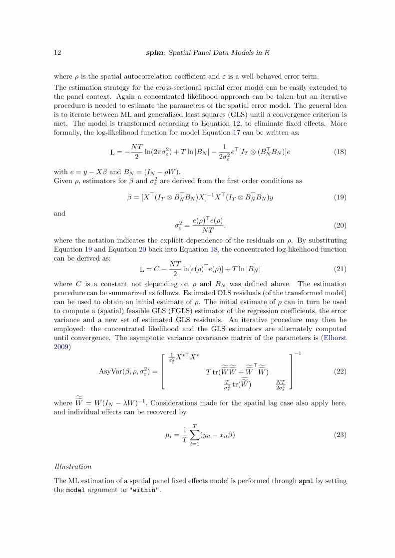
12 splm: Spatial Panel Data Models in R
where ρ is the spatial autocorrelation coefficient and ε is a well-behaved error term.
The estimation strategy for the cross-sectional spatial error model can be easily extended tothe panel context. Again a concentrated likelihood approach can be taken but an iterativeprocedure is needed to estimate the parameters of the spatial error model. The general ideais to iterate between ML and generalized least squares (GLS) until a convergence criterion ismet. The model is transformed according to Equation 12, to eliminate fixed effects. Moreformally, the log-likelihood function for model Equation 17 can be written as:
L = −NT2
ln(2πσ2ε) + T ln |BN | −1
2σ2εe>[IT ⊗ (B>NBN )]e (18)
with e = y −Xβ and BN = (IN − ρW ).Given ρ, estimators for β and σ2ε are derived from the first order conditions as
β = [X>(IT ⊗B>NBN )X]−1X>(IT ⊗B>NBN )y (19)
and
σ2ε =e(ρ)>e(ρ)
NT. (20)
where the notation indicates the explicit dependence of the residuals on ρ. By substitutingEquation 19 and Equation 20 back into Equation 18, the concentrated log-likelihood functioncan be derived as:
L = C − NT
2ln[e(ρ)>e(ρ)] + T ln |BN | (21)
where C is a constant not depending on ρ and BN was defined above. The estimationprocedure can be summarized as follows. Estimated OLS residuals (of the transformed model)can be used to obtain an initial estimate of ρ. The initial estimate of ρ can in turn be usedto compute a (spatial) feasible GLS (FGLS) estimator of the regression coefficients, the errorvariance and a new set of estimated GLS residuals. An iterative procedure may then beemployed: the concentrated likelihood and the GLS estimators are alternately computeduntil convergence. The asymptotic variance covariance matrix of the parameters is (Elhorst2009)
AsyVar(β, ρ, σ2ε) =
1σ2εX∗>X∗
T tr(˜W˜W +
˜W>˜W )
Tσ2ε
tr(˜W ) NT
2σ4ε
−1
(22)
where˜W = W (IN − λW )−1. Considerations made for the spatial lag case also apply here,
and individual effects can be recovered by
µi =1
T
T∑t=1
(yit − xitβ) (23)
Illustration
The ML estimation of a spatial panel fixed effects model is performed through spml by settingthe model argument to "within".

Journal of Statistical Software 13
The spml function allows the estimation of a model specified in terms of both spatial effects.This can be done by combining the arguments lag and spatial.error as in the followingexample:
R> sararfemod <- spml(formula = fm, data = Produc, index = NULL,
+ listw = usalw, lag = TRUE, spatial.error = "b", model = "within",
+ effect = "individual", method = "eigen", na.action = na.fail,
+ quiet = TRUE, zero.policy = NULL, interval = NULL,
+ tol.solve = 1e-10, control = list(), legacy = FALSE)
R> summary(sararfemod)
Spatial panel fixed effects sarar model
Call:
spml(formula = fm, data = Produc, index = NULL, listw = usalw,
model = "within", effect = "individual", lag = TRUE, spatial.error = "b",
method = "eigen", na.action = na.fail, quiet = TRUE, zero.policy = NULL,
interval = NULL, tol.solve = 1e-10, control = list(), legacy = FALSE)
Residuals:
Min. 1st Qu. Median 3rd Qu. Max.
-0.1340 -0.0221 -0.0032 0.0172 0.1750
Coefficients:
Estimate Std. Error t-value Pr(>|t|)
rho 0.4553116 0.0504043 9.0332 < 2.2e-16 ***
lambda 0.0885760 0.0300044 2.9521 0.003156 **
log(pcap) -0.0103497 0.0252725 -0.4095 0.682156
log(pc) 0.1905781 0.0230505 8.2678 < 2.2e-16 ***
log(emp) 0.7552372 0.0277505 27.2152 < 2.2e-16 ***
unemp -0.0030613 0.0010293 -2.9741 0.002939 **
---
Signif. codes: 0 '***' 0.001 '**' 0.01 '*' 0.05 '.' 0.1 ' ' 1
As is well known, the within transformation eliminates the individual effects. Thus, froman empirical point of view, it also makes the two specifications (individuals effects are/arenot spatially autocorrelated) indistinguishable. Therefore, the argument spatial.error canequivalently take the values b or kkp, thus leading to the estimation of the same specification.
There are specific arguments to spml for spatial within models that can be passed on throughthe special ‘...’ argument. The argument method sets the technique for the calculation of thedeterminant. The default ("eigen") is to express the Jacobian in terms of the eigenvalues ofthe spatial weights matrix. Other available options include methods based on sparse matrices("spam", "Matrix" or "LU"), and the Chebyshev ("Chebyshev") and Monte Carlo ("MC")approximations.
As an example, to estimate a model with only individual fixed effects:
R> sarfemod <- spml(formula = fm, data = Produc, index = NULL, listw = usalw,
+ model = "within", effect = "individual", method = "eigen",
14 splm: Spatial Panel Data Models in R
+ na.action = na.fail, quiet = TRUE, zero.policy = NULL, interval = NULL,
+ tol.solve = 1e-10, control = list(), legacy = FALSE)
R> summary(sarfemod)
Spatial panel fixed effects error model
Call:
spml(formula = fm, data = Produc, index = NULL, listw = usalw,
model = "within", effect = "individual", method = "eigen",
na.action = na.fail, quiet = TRUE, zero.policy = NULL, interval = NULL,
tol.solve = 1e-10, control = list(), legacy = FALSE)
Residuals:
Min. 1st Qu. Median 3rd Qu. Max.
-0.1250 -0.0238 -0.0035 0.0171 0.1880
Coefficients:
Estimate Std. Error t-value Pr(>|t|)
rho 0.5574013 0.0330749 16.8527 < 2e-16 ***
log(pcap) 0.0051438 0.0250109 0.2057 0.83705
log(pc) 0.2053026 0.0231427 8.8712 < 2e-16 ***
log(emp) 0.7822540 0.0278057 28.1328 < 2e-16 ***
unemp -0.0022317 0.0010709 -2.0839 0.03717 *
---
Signif. codes: 0 '***' 0.001 '**' 0.01 '*' 0.05 '.' 0.1 ' ' 1
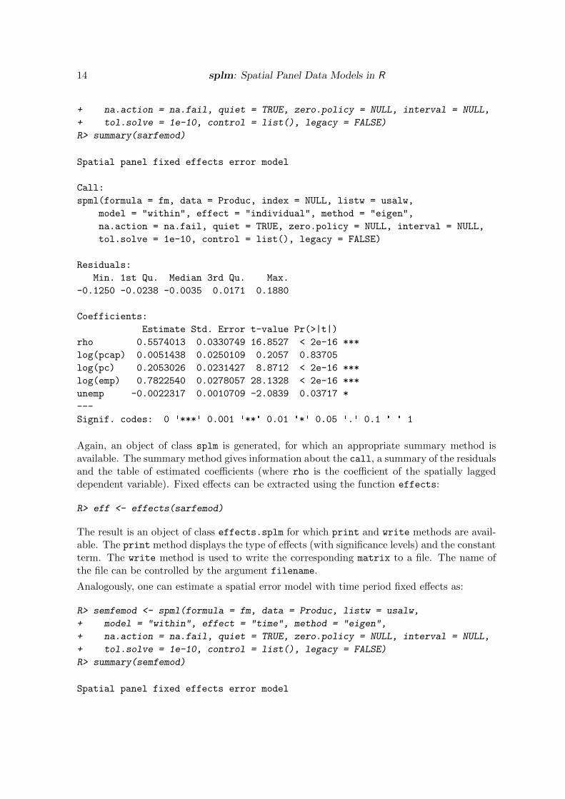
Again, an object of class splm is generated, for which an appropriate summary method isavailable. The summary method gives information about the call, a summary of the residualsand the table of estimated coefficients (where rho is the coefficient of the spatially laggeddependent variable). Fixed effects can be extracted using the function effects:
R> eff <- effects(sarfemod)
The result is an object of class effects.splm for which print and write methods are avail-able. The print method displays the type of effects (with significance levels) and the constantterm. The write method is used to write the corresponding matrix to a file. The name ofthe file can be controlled by the argument filename.
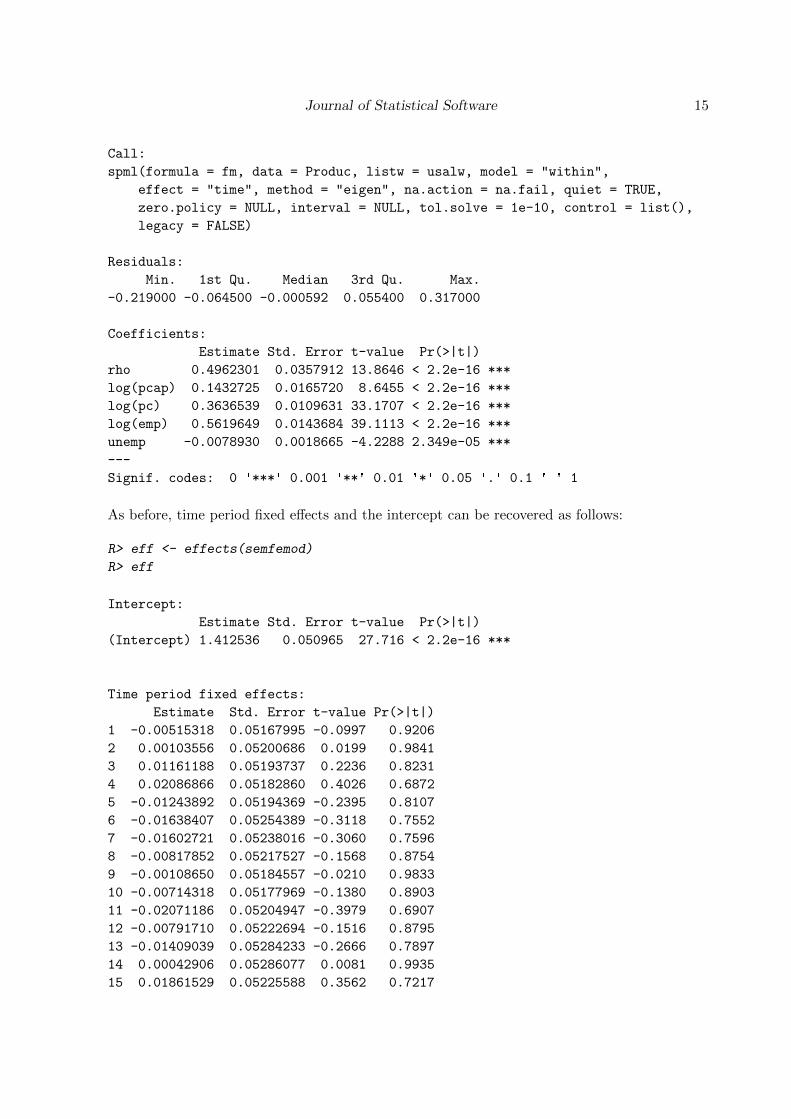
Analogously, one can estimate a spatial error model with time period fixed effects as:
R> semfemod <- spml(formula = fm, data = Produc, listw = usalw,
+ model = "within", effect = "time", method = "eigen",
+ na.action = na.fail, quiet = TRUE, zero.policy = NULL, interval = NULL,
+ tol.solve = 1e-10, control = list(), legacy = FALSE)
R> summary(semfemod)
Spatial panel fixed effects error model
Journal of Statistical Software 15
Call:
spml(formula = fm, data = Produc, listw = usalw, model = "within",
effect = "time", method = "eigen", na.action = na.fail, quiet = TRUE,
zero.policy = NULL, interval = NULL, tol.solve = 1e-10, control = list(),
legacy = FALSE)
Residuals:
Min. 1st Qu. Median 3rd Qu. Max.
-0.219000 -0.064500 -0.000592 0.055400 0.317000
Coefficients:
Estimate Std. Error t-value Pr(>|t|)
rho 0.4962301 0.0357912 13.8646 < 2.2e-16 ***
log(pcap) 0.1432725 0.0165720 8.6455 < 2.2e-16 ***
log(pc) 0.3636539 0.0109631 33.1707 < 2.2e-16 ***
log(emp) 0.5619649 0.0143684 39.1113 < 2.2e-16 ***
unemp -0.0078930 0.0018665 -4.2288 2.349e-05 ***
---
Signif. codes: 0 '***' 0.001 '**' 0.01 '*' 0.05 '.' 0.1 ' ' 1
As before, time period fixed effects and the intercept can be recovered as follows:
R> eff <- effects(semfemod)
R> eff
Intercept:
Estimate Std. Error t-value Pr(>|t|)
(Intercept) 1.412536 0.050965 27.716 < 2.2e-16 ***
Time period fixed effects:
Estimate Std. Error t-value Pr(>|t|)
1 -0.00515318 0.05167995 -0.0997 0.9206
2 0.00103556 0.05200686 0.0199 0.9841
3 0.01161188 0.05193737 0.2236 0.8231
4 0.02086866 0.05182860 0.4026 0.6872
5 -0.01243892 0.05194369 -0.2395 0.8107
6 -0.01638407 0.05254389 -0.3118 0.7552
7 -0.01602721 0.05238016 -0.3060 0.7596
8 -0.00817852 0.05217527 -0.1568 0.8754
9 -0.00108650 0.05184557 -0.0210 0.9833
10 -0.00714318 0.05177969 -0.1380 0.8903
11 -0.02071186 0.05204947 -0.3979 0.6907
12 -0.00791710 0.05222694 -0.1516 0.8795
13 -0.01409039 0.05284233 -0.2666 0.7897
14 0.00042906 0.05286077 0.0081 0.9935
15 0.01861529 0.05225588 0.3562 0.7217
16 splm: Spatial Panel Data Models in R
16 0.02531034 0.05216326 0.4852 0.6275
17 0.03126013 0.05219134 0.5990 0.5492
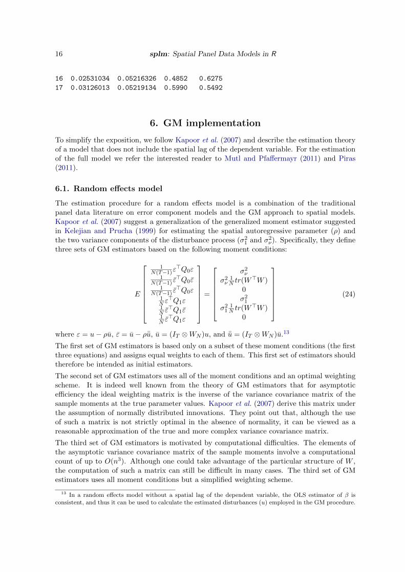
6. GM implementation
To simplify the exposition, we follow Kapoor et al. (2007) and describe the estimation theoryof a model that does not include the spatial lag of the dependent variable. For the estimationof the full model we refer the interested reader to Mutl and Pfaffermayr (2011) and Piras(2011).
6.1. Random effects model
The estimation procedure for a random effects model is a combination of the traditionalpanel data literature on error component models and the GM approach to spatial models.Kapoor et al. (2007) suggest a generalization of the generalized moment estimator suggestedin Kelejian and Prucha (1999) for estimating the spatial autoregressive parameter (ρ) andthe two variance components of the disturbance process (σ21 and σ2ν). Specifically, they definethree sets of GM estimators based on the following moment conditions:
E
1N(T−1)ε
>Q0ε1
N(T−1) ε>Q0ε
1N(T−1) ε
>Q0ε1N ε>Q1ε
1N ε>Q1ε
1N ε>Q1ε
=
σ2νσ2ν
1N tr(W
>W )0σ21
σ211N tr(W
>W )0
(24)
where ε = u− ρu, ε = u− ρ¯u, u = (IT ⊗WN )u, and ¯u = (IT ⊗WN )u.13
The first set of GM estimators is based only on a subset of these moment conditions (the firstthree equations) and assigns equal weights to each of them. This first set of estimators shouldtherefore be intended as initial estimators.
The second set of GM estimators uses all of the moment conditions and an optimal weightingscheme. It is indeed well known from the theory of GM estimators that for asymptoticefficiency the ideal weighting matrix is the inverse of the variance covariance matrix of thesample moments at the true parameter values. Kapoor et al. (2007) derive this matrix underthe assumption of normally distributed innovations. They point out that, although the useof such a matrix is not strictly optimal in the absence of normality, it can be viewed as areasonable approximation of the true and more complex variance covariance matrix.
The third set of GM estimators is motivated by computational difficulties. The elements ofthe asymptotic variance covariance matrix of the sample moments involve a computationalcount of up to O(n3). Although one could take advantage of the particular structure of W ,the computation of such a matrix can still be difficult in many cases. The third set of GMestimators uses all moment conditions but a simplified weighting scheme.
13 In a random effects model without a spatial lag of the dependent variable, the OLS estimator of β isconsistent, and thus it can be used to calculate the estimated disturbances (u) employed in the GM procedure.
Journal of Statistical Software 17
Using any of the previously defined estimators for the spatial coefficient and the variancecomponents, a feasible GLS estimator of β can be defined based on a spatial Cochrane-Orcutttype transformation of the original model. However, following the classical error componentliterature, a convenient way of calculating the GLS estimator is to further transform the(spatially transformed) model by premultiplying it by INT − θQ1, where θ = 1− σν/σ1. Thefeasible GLS estimator is then identical to an OLS calculated on the “doubly” transformedmodel. Finally, small sample inference can be based on the following expression for thecoefficient’s variance-covariance matrix
Ψ = (X∗>Ω−1ε X∗)−1 (25)
where the variables X∗ can be viewed as the result of a spatial Cochrane-Orcutt type trans-formation of the original model, and X∗ and Ω−1ε depend on the estimated values of ρ, σ2νand σ21 respectively.
Illustration
spgm is a general interface to estimate various nested specifications of the model presentedin Section 4. The function also gives the possibility of including additional (other than thespatial lag) endogenous variables. To make sure that we are estimating a random effectsspecification, the argument effects should be set to "random". Along with a mandatoryformula object to describe the model, the function consists of a series of optional arguments.Among them, there are two logical vectors that control for the basic model specification:spatial.error and lag. When both arguments are FALSE, an endogenous variable shouldbe specified (endog) along with a set of instruments. In this particular case, the functionuses an estimation engine (ivsplm) to perform instrumental variables estimation for paneldata models. The argument method can be used to select among different estimators.14
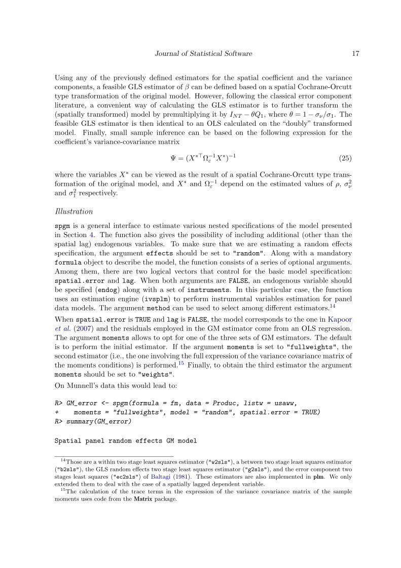
When spatial.error is TRUE and lag is FALSE, the model corresponds to the one in Kapooret al. (2007) and the residuals employed in the GM estimator come from an OLS regression.The argument moments allows to opt for one of the three sets of GM estimators. The defaultis to perform the initial estimator. If the argument moments is set to "fullweights", thesecond estimator (i.e., the one involving the full expression of the variance covariance matrix ofthe moments conditions) is performed.15 Finally, to obtain the third estimator the argumentmoments should be set to "weights".
On Munnell’s data this would lead to:
R> GM_error <- spgm(formula = fm, data = Produc, listw = usaww,
+ moments = "fullweights", model = "random", spatial.error = TRUE)
R> summary(GM_error)
Spatial panel random effects GM model
14Those are a within two stage least squares estimator ("w2sls"), a between two stage least squares estimator("b2sls"), the GLS random effects two stage least squares estimator ("g2sls"), and the error component twostages least squares ("ec2sls") of Baltagi (1981). These estimators are also implemented in plm. We onlyextended them to deal with the case of a spatially lagged dependent variable.
15The calculation of the trace terms in the expression of the variance covariance matrix of the samplemoments uses code from the Matrix package.
18 splm: Spatial Panel Data Models in R
Call:
spgm(formula = fm, data = Produc, listw = usaww, model = "random",
spatial.error = TRUE, moments = "fullweights")
Residuals:
Min. 1st Qu. Median Mean 3rd Qu. Max.
-0.26600 -0.06560 -0.00717 -0.00480 0.04850 0.45900
Estimated spatial coefficient, variance components and theta:
Estimate
rho 0.5480458
sigma^2_v 0.0011228
sigma^2_1 0.0880980
theta 0.8871080
Coefficients:
Estimate Std. Error t-value Pr(>|t|)
(Intercept) 2.2273109 0.1350925 16.4873 < 2.2e-16 ***
log(pcap) 0.0540235 0.0219720 2.4587 0.013942 *
log(pc) 0.2565950 0.0209339 12.2574 < 2.2e-16 ***
log(emp) 0.7278192 0.0252306 28.8466 < 2.2e-16 ***
unemp -0.0038108 0.0011004 -3.4631 0.000534 ***
---
Signif. codes: 0 '***' 0.001 '**' 0.01 '*' 0.05 '.' 0.1 ' ' 1
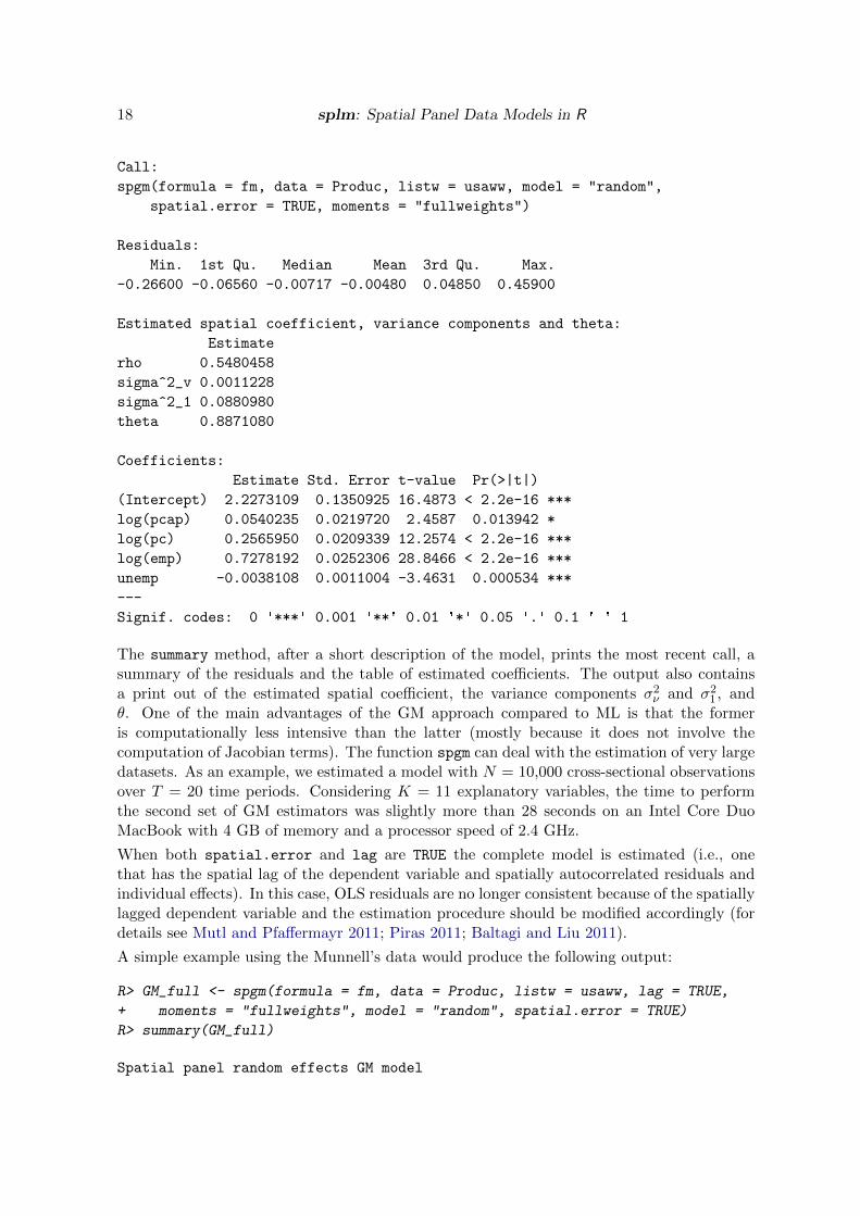
The summary method, after a short description of the model, prints the most recent call, asummary of the residuals and the table of estimated coefficients. The output also containsa print out of the estimated spatial coefficient, the variance components σ2ν and σ21, andθ. One of the main advantages of the GM approach compared to ML is that the formeris computationally less intensive than the latter (mostly because it does not involve thecomputation of Jacobian terms). The function spgm can deal with the estimation of very largedatasets. As an example, we estimated a model with N = 10,000 cross-sectional observationsover T = 20 time periods. Considering K = 11 explanatory variables, the time to performthe second set of GM estimators was slightly more than 28 seconds on an Intel Core DuoMacBook with 4 GB of memory and a processor speed of 2.4 GHz.
When both spatial.error and lag are TRUE the complete model is estimated (i.e., onethat has the spatial lag of the dependent variable and spatially autocorrelated residuals andindividual effects). In this case, OLS residuals are no longer consistent because of the spatiallylagged dependent variable and the estimation procedure should be modified accordingly (fordetails see Mutl and Pfaffermayr 2011; Piras 2011; Baltagi and Liu 2011).
A simple example using the Munnell’s data would produce the following output:
R> GM_full <- spgm(formula = fm, data = Produc, listw = usaww, lag = TRUE,
+ moments = "fullweights", model = "random", spatial.error = TRUE)
R> summary(GM_full)
Spatial panel random effects GM model
Journal of Statistical Software 19
Call:
spgm(formula = fm, data = Produc, listw = usaww, model = "random",
lag = TRUE, spatial.error = TRUE, moments = "fullweights")
Residuals:
Min. 1st Qu. Median Mean 3rd Qu. Max.
-0.27400 -0.06050 -0.00206 -0.00194 0.05260 0.47100
Estimated spatial coefficient, variance components and theta:
Estimate
rho 0.3409051
sigma^2_v 0.0011002
sigma^2_1 0.0928450
theta 0.8911412
Coefficients:
Estimate Std. Error t-value Pr(>|t|)
lambda 0.02185030 0.01350631 1.6178 0.1057
(Intercept) 2.01866772 0.16797180 12.0179 < 2.2e-16 ***
log(pcap) 0.04668406 0.02244161 2.0802 0.0375 *
log(pc) 0.26596681 0.02036336 13.0610 < 2.2e-16 ***
log(emp) 0.72160852 0.02473123 29.1780 < 2.2e-16 ***
unemp -0.00513207 0.00097481 -5.2647 1.404e-07 ***
---
Signif. codes: 0 '***' 0.001 '**' 0.01 '*' 0.05 '.' 0.1 ' ' 1
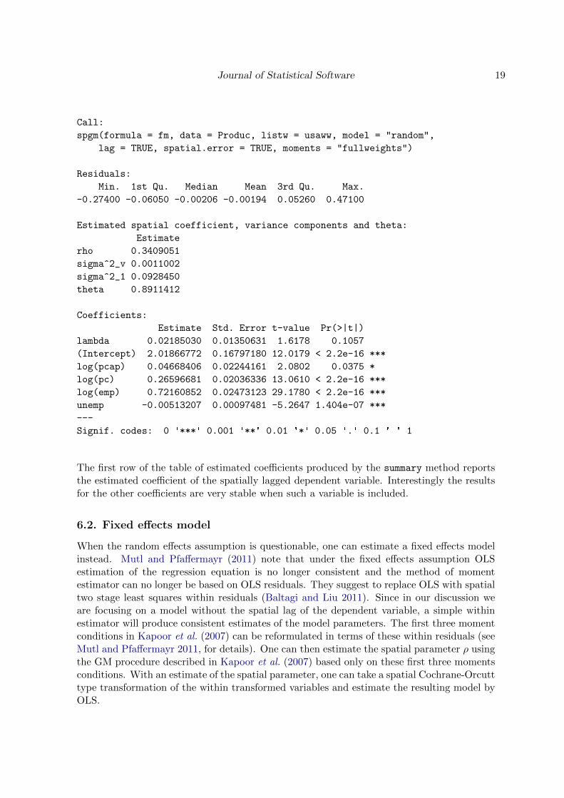
The first row of the table of estimated coefficients produced by the summary method reportsthe estimated coefficient of the spatially lagged dependent variable. Interestingly the resultsfor the other coefficients are very stable when such a variable is included.
6.2. Fixed effects model
When the random effects assumption is questionable, one can estimate a fixed effects modelinstead. Mutl and Pfaffermayr (2011) note that under the fixed effects assumption OLSestimation of the regression equation is no longer consistent and the method of momentestimator can no longer be based on OLS residuals. They suggest to replace OLS with spatialtwo stage least squares within residuals (Baltagi and Liu 2011). Since in our discussion weare focusing on a model without the spatial lag of the dependent variable, a simple withinestimator will produce consistent estimates of the model parameters. The first three momentconditions in Kapoor et al. (2007) can be reformulated in terms of these within residuals (seeMutl and Pfaffermayr 2011, for details). One can then estimate the spatial parameter ρ usingthe GM procedure described in Kapoor et al. (2007) based only on these first three momentsconditions. With an estimate of the spatial parameter, one can take a spatial Cochrane-Orcutttype transformation of the within transformed variables and estimate the resulting model byOLS.
20 splm: Spatial Panel Data Models in R
Illustration
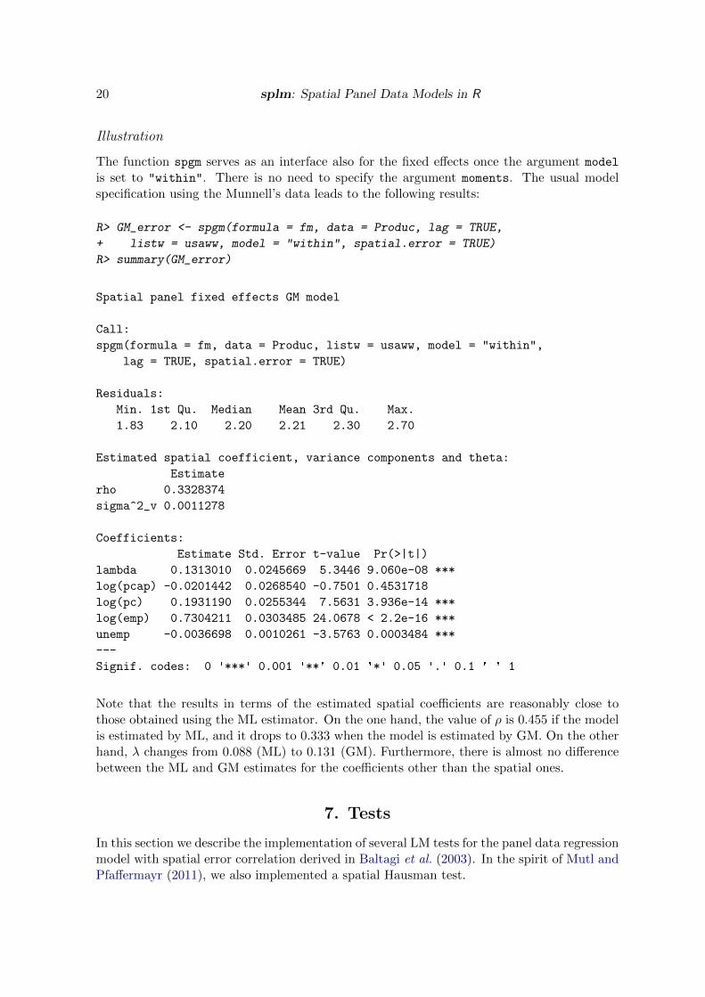
The function spgm serves as an interface also for the fixed effects once the argument model
is set to "within". There is no need to specify the argument moments. The usual modelspecification using the Munnell’s data leads to the following results:
R> GM_error <- spgm(formula = fm, data = Produc, lag = TRUE,
+ listw = usaww, model = "within", spatial.error = TRUE)
R> summary(GM_error)
Spatial panel fixed effects GM model
Call:
spgm(formula = fm, data = Produc, listw = usaww, model = "within",
lag = TRUE, spatial.error = TRUE)
Residuals:
Min. 1st Qu. Median Mean 3rd Qu. Max.
1.83 2.10 2.20 2.21 2.30 2.70
Estimated spatial coefficient, variance components and theta:
Estimate
rho 0.3328374
sigma^2_v 0.0011278
Coefficients:
Estimate Std. Error t-value Pr(>|t|)
lambda 0.1313010 0.0245669 5.3446 9.060e-08 ***
log(pcap) -0.0201442 0.0268540 -0.7501 0.4531718
log(pc) 0.1931190 0.0255344 7.5631 3.936e-14 ***
log(emp) 0.7304211 0.0303485 24.0678 < 2.2e-16 ***
unemp -0.0036698 0.0010261 -3.5763 0.0003484 ***
---
Signif. codes: 0 '***' 0.001 '**' 0.01 '*' 0.05 '.' 0.1 ' ' 1
Note that the results in terms of the estimated spatial coefficients are reasonably close tothose obtained using the ML estimator. On the one hand, the value of ρ is 0.455 if the modelis estimated by ML, and it drops to 0.333 when the model is estimated by GM. On the otherhand, λ changes from 0.088 (ML) to 0.131 (GM). Furthermore, there is almost no differencebetween the ML and GM estimates for the coefficients other than the spatial ones.
7. Tests
In this section we describe the implementation of several LM tests for the panel data regressionmodel with spatial error correlation derived in Baltagi et al. (2003). In the spirit of Mutl andPfaffermayr (2011), we also implemented a spatial Hausman test.
Journal of Statistical Software 21
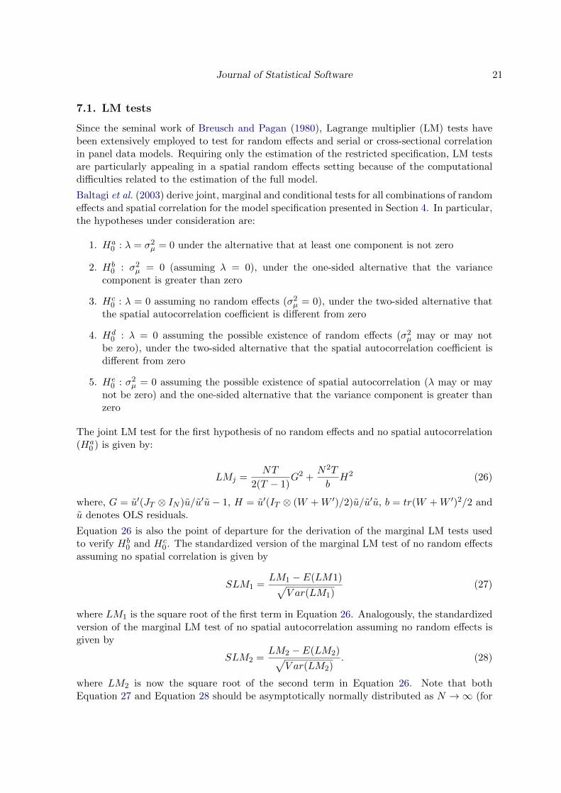
7.1. LM tests
Since the seminal work of Breusch and Pagan (1980), Lagrange multiplier (LM) tests havebeen extensively employed to test for random effects and serial or cross-sectional correlationin panel data models. Requiring only the estimation of the restricted specification, LM testsare particularly appealing in a spatial random effects setting because of the computationaldifficulties related to the estimation of the full model.
Baltagi et al. (2003) derive joint, marginal and conditional tests for all combinations of randomeffects and spatial correlation for the model specification presented in Section 4. In particular,the hypotheses under consideration are:
1. Ha0 : λ = σ2µ = 0 under the alternative that at least one component is not zero
2. Hb0 : σ2µ = 0 (assuming λ = 0), under the one-sided alternative that the variance
component is greater than zero
3. Hc0 : λ = 0 assuming no random effects (σ2µ = 0), under the two-sided alternative that
the spatial autocorrelation coefficient is different from zero
4. Hd0 : λ = 0 assuming the possible existence of random effects (σ2µ may or may not
be zero), under the two-sided alternative that the spatial autocorrelation coefficient isdifferent from zero
5. He0 : σ2µ = 0 assuming the possible existence of spatial autocorrelation (λ may or may
not be zero) and the one-sided alternative that the variance component is greater thanzero
The joint LM test for the first hypothesis of no random effects and no spatial autocorrelation(Ha
0 ) is given by:
LMj =NT
2(T − 1)G2 +
N2T
bH2 (26)
where, G = u′(JT ⊗ IN )u/u′u− 1, H = u′(IT ⊗ (W +W ′)/2)u/u′u, b = tr(W +W ′)2/2 andu denotes OLS residuals.
Equation 26 is also the point of departure for the derivation of the marginal LM tests usedto verify Hb
0 and Hc0. The standardized version of the marginal LM test of no random effects
assuming no spatial correlation is given by
SLM1 =LM1 − E(LM1)√
V ar(LM1)(27)
where LM1 is the square root of the first term in Equation 26. Analogously, the standardizedversion of the marginal LM test of no spatial autocorrelation assuming no random effects isgiven by
SLM2 =LM2 − E(LM2)√
V ar(LM2). (28)
where LM2 is now the square root of the second term in Equation 26. Note that bothEquation 27 and Equation 28 should be asymptotically normally distributed as N →∞ (for

22 splm: Spatial Panel Data Models in R
fixed T ) under Hb0 and Hc
0 respectively.16 Based on Equation 27 and Equation 28, a usefulone-sided test statistic for Ha
0 : λ = σ2µ = 0 can be derived as:
LMH = (LM1 + LM2)/√
2 (29)
which is asymptotically distributed N(0, 1). A test for the joint null hypothesis can, therefore,be based on the following decision rule:
χ2m =
LM2
1 + LM22 if LM1 > 0, LM2 > 0
LM21 if LM1 > 0, LM2 ≤ 0
LM22 if LM1 ≤ 0, LM2 > 0
0 if LM1 ≤ 0, LM2 ≤ 0
Under the null the test statistic χ2m has a mixed χ2-distribution given by:
χ2m = (1/4)χ2(0) + (1/2)χ2(1) + (1/4)χ2(2) (30)
When using LM2, one is assuming that random individual effects do not exist. However,especially when the variance component is large, this may lead to incorrect inference. Thisis why Baltagi et al. (2003) derive a conditional LM test against the spatial autocorrelationcoefficient being zero assuming that the variance component may or may not be zero. Theexpression for the test assumes the following form:
LMλ =D(λ)2
[(T − 1) + σ4ν/σ41]b
(31)
where, D(λ)2 = 12 u′[σ4ν
σ41(JT ⊗ (W ′ +W )) + 1
σ4ν(ET ⊗ (W ′ +W ))
]u. Also, σ41 = u′(JT ⊗
IN )u/N , σ4ν = u′(ET ⊗IN )u/N(T −1) and, contrary to previous tests that use OLS residuals,the residuals u are ML. The comparative disadvantage of this last test is that its implemen-tation is slightly more complicated because it is based on ML residuals. A one sided test issimply obtained by taking the square root of Equation 31. The resulting test statistic shouldbe asymptotically distributed N(0, 1). Similarly, when using LM1 one is assuming no spatialerror correlation. This assumption may lead to incorrect inferences particularly when λ isnot very close to zero. A conditional LM test assuming the possible existence of spatial errorcorrelation can be derived as:
LMµ = (Dµ)2(
2σ4νT
)(TNσ4νec−Nσ4νd2 − T σ4νg2e+ 2σ4νghd− σ4νh2c)−1 × (Nσ4νc− σ4νg2)
where, g = tr[(W ′B + B′W )(B′B)−1], h = tr[B′B], d = tr[(W ′B + B′W )], c = tr[((W ′B +B′W )(B′B)−1)2] and e = tr[(B′B)2]. A one-sided test can be defined by taking the squareroot of Equation 32 based on ML residuals. The test statistic should be asymptoticallydistributed N(0, 1).
Illustration
The bsktest function can compute the joint, marginal or conditional tests for random effectsand spatial error correlation. There are currently five options to the argument test, corre-sponding to the tests in the Baltagi et al. (2003): "LM1", "LM2", "LMJOINT", "CLMlambda", and
16 For details on the expressions for the expected values and the variances of both tests see Baltagi et al.(2003).
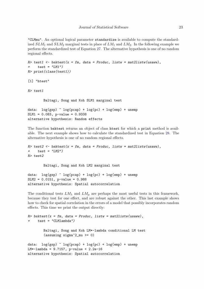
Journal of Statistical Software 23
"CLMmu". An optional logical parameter standardize is available to compute the standard-ized SLM1 and SLM2 marginal tests in place of LM1 and LM2. In the following example weperform the standardized test of Equation 27. The alternative hypothesis is one of no randomregional effects.
R> test1 <- bsktest(x = fm, data = Produc, listw = mat2listw(usaww),
+ test = "LM1")
R> print(class(test1))
[1] "htest"
R> test1
Baltagi, Song and Koh SLM1 marginal test
data: log(gsp) ~ log(pcap) + log(pc) + log(emp) + unemp
SLM1 = 0.083, p-value = 0.9338
alternative hypothesis: Random effects
The function bsktest returns an object of class htest for which a print method is avail-able. The next example shows how to calculate the standardized test in Equation 28. Thealternative hypothesis is one of no random regional effects.
R> test2 <- bsktest(x = fm, data = Produc, listw = mat2listw(usaww),
+ test = "LM2")
R> test2
Baltagi, Song and Koh LM2 marginal test
data: log(gsp) ~ log(pcap) + log(pc) + log(emp) + unemp
SLM2 = 0.0151, p-value = 0.988
alternative hypothesis: Spatial autocorrelation
The conditional tests LMλ and LMµ are perhaps the most useful tests in this framework,because they test for one effect, and are robust against the other. This last example showshow to check for spatial correlation in the errors of a model that possibly incorporates randomeffects. This time we print the output directly:
R> bsktest(x = fm, data = Produc, listw = mat2listw(usaww),
+ test = "CLMlambda")
Baltagi, Song and Koh LM*-lambda conditional LM test
(assuming sigma^2_mu >= 0)
data: log(gsp) ~ log(pcap) + log(pc) + log(emp) + unemp
LM*-lambda = 9.7157, p-value < 2.2e-16
alternative hypothesis: Spatial autocorrelation

24 splm: Spatial Panel Data Models in R
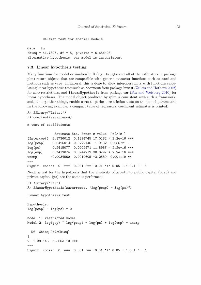
7.2. Spatial Hausman test
The Hausman test (Hausman 1978) compares random and fixed effects estimators and testswhether or not the random effects assumption is supported by the data. Mutl and Pfaffermayr(2011) show how to extend this procedure to a spatial framework. The Hausman test statistictakes the form
H = NT (θFGLS − θW )>(ΣW − ΣFGLS)−1(θFGLS − θW ) (32)
where θFGLS and θW are, respectively, the spatial GLS and within estimators, and ΣW andΣFGLS the corresponding estimates of the coefficients’ variance covariance matrices. H isasymptotically distributed χ2 with k degrees of freedom where k is the number of regressorsin the model.
Illustration
The method sphtest computes the spatial Hausman test described in the previous sec-tion. The argument can either be a formula describing the model to be estimated, oran object of class splm. If the argument is a formula, it should be specified along withthree additional arguments: an object of class listw, a description of the model to be esti-mated (spatial.model) and the estimation method (method). Furthermore, if the estimationmethod is ML, the argument errors indicates which specification of the error term has to beconsidered.
The following example illustrates the function when the argument is a formula. We estimatea model without a spatial lag but with an autocorrelated error term. Since the estimationmethod is "GM" there is no need to specify the structure of the error term.
R> test1 <- sphtest(x = fm, data = Produc, listw = mat2listw(usaww),
+ spatial.model = "error", method = "GM")
R> test1
Hausman test for spatial models
data: x
chisq = 7.4824, df = 4, p-value = 0.1125
alternative hypothesis: one model is inconsistent
The function sphtsest returns an object of class htest for which a print method is available.The next example shows that if the two models are estimated separately, the two objects ofclass splm can be given as arguments to the function.
R> mod1 <- spgm(formula = fm, data = Produc, listw = usaww, lag = TRUE,
+ moments = "fullweights", model = "random", spatial.error = TRUE)
R> mod2 <- spgm(formula = fm, data = Produc, listw = usaww, lag = TRUE,
+ model = "within", spatial.error = TRUE)
R> test2 <- sphtest(x = mod1, x2 = mod2)
R> test2
Journal of Statistical Software 25
Hausman test for spatial models
data: fm
chisq = 41.7396, df = 5, p-value = 6.65e-08
alternative hypothesis: one model is inconsistent
7.3. Linear hypothesis testing
Many functions for model estimation in R (e.g., lm, glm and all of the estimators in packageplm) return objects that are compatible with generic extractor functions such as coef andmethods such as vcov. In general, this is done to allow interoperability with functions calcu-lating linear hypothesis tests such as coeftest from package lmtest (Zeileis and Hothorn 2002)for zero-restrictions, and linearHypothesis from package car (Fox and Weisberg 2010) forlinear hypotheses. The model object produced by splm is consistent with such a framework,and, among other things, enable users to perform restriction tests on the model parameters.In the following example, a compact table of regressors’ coefficient estimates is printed:
R> library("lmtest")
R> coeftest(sararremod)
z test of coefficients:
Estimate Std. Error z value Pr(>|z|)
(Intercept) 2.3736012 0.1394745 17.0182 < 2.2e-16 ***
log(pcap) 0.0425013 0.0222146 1.9132 0.055721 .
log(pc) 0.2415077 0.0202971 11.8987 < 2.2e-16 ***
log(emp) 0.7419074 0.0244212 30.3797 < 2.2e-16 ***
unemp -0.0034560 0.0010605 -3.2589 0.001119 **
---
Signif. codes: 0 '***' 0.001 '**' 0.01 '*' 0.05 '.' 0.1 ' ' 1
Next, a test for the hypothesis that the elasticity of growth to public capital (pcap) andprivate capital (pc) are the same is performed:
R> library("car")
R> linearHypothesis(sararremod, "log(pcap) = log(pc)")
Linear hypothesis test
Hypothesis:
log(pcap) - log(pc) = 0
Model 1: restricted model
Model 2: log(gsp) ~ log(pcap) + log(pc) + log(emp) + unemp
Df Chisq Pr(>Chisq)
1
2 1 38.145 6.566e-10 ***
---
Signif. codes: 0 '***' 0.001 '**' 0.01 '*' 0.05 '.' 0.1 ' ' 1
26 splm: Spatial Panel Data Models in R
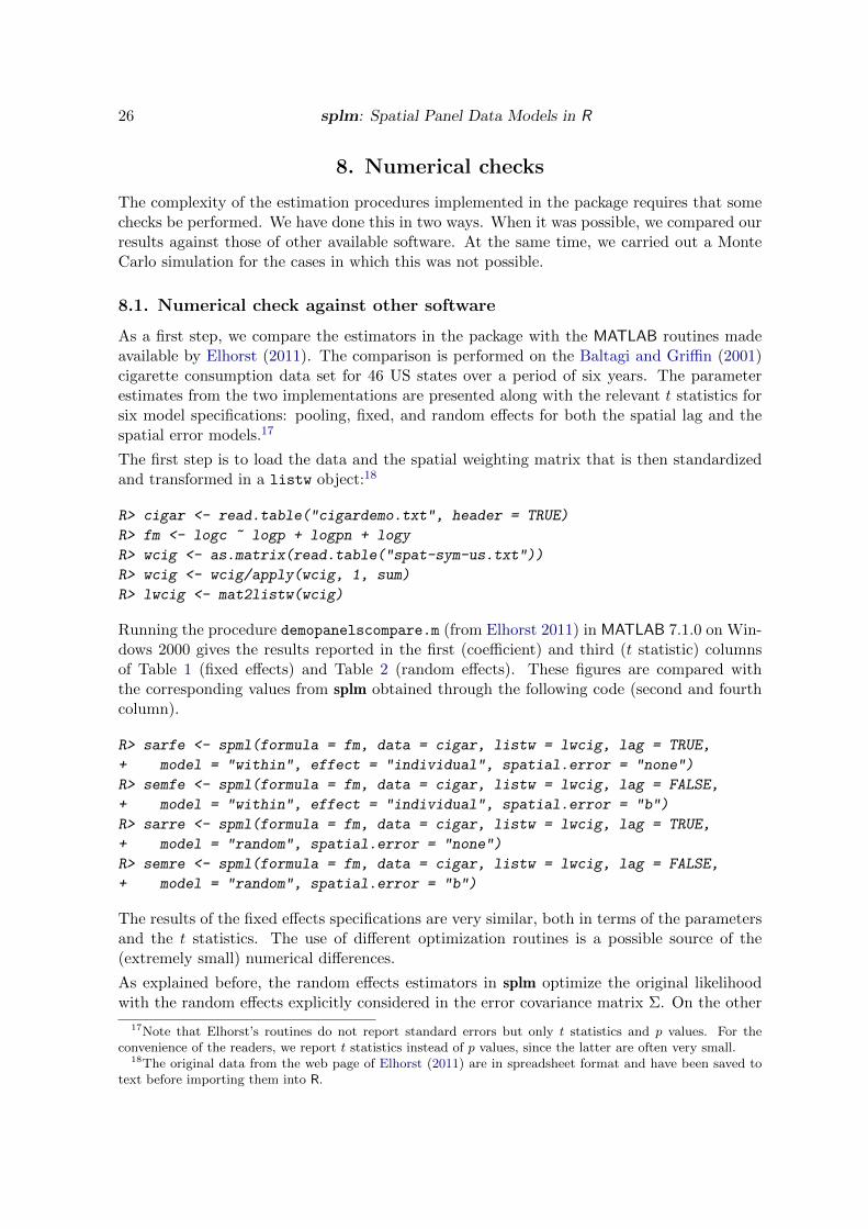
8. Numerical checks
The complexity of the estimation procedures implemented in the package requires that somechecks be performed. We have done this in two ways. When it was possible, we compared ourresults against those of other available software. At the same time, we carried out a MonteCarlo simulation for the cases in which this was not possible.
8.1. Numerical check against other software
As a first step, we compare the estimators in the package with the MATLAB routines madeavailable by Elhorst (2011). The comparison is performed on the Baltagi and Griffin (2001)cigarette consumption data set for 46 US states over a period of six years. The parameterestimates from the two implementations are presented along with the relevant t statistics forsix model specifications: pooling, fixed, and random effects for both the spatial lag and thespatial error models.17
The first step is to load the data and the spatial weighting matrix that is then standardizedand transformed in a listw object:18
R> cigar <- read.table("cigardemo.txt", header = TRUE)
R> fm <- logc ~ logp + logpn + logy
R> wcig <- as.matrix(read.table("spat-sym-us.txt"))
R> wcig <- wcig/apply(wcig, 1, sum)
R> lwcig <- mat2listw(wcig)
Running the procedure demopanelscompare.m (from Elhorst 2011) in MATLAB 7.1.0 on Win-dows 2000 gives the results reported in the first (coefficient) and third (t statistic) columnsof Table 1 (fixed effects) and Table 2 (random effects). These figures are compared withthe corresponding values from splm obtained through the following code (second and fourthcolumn).
R> sarfe <- spml(formula = fm, data = cigar, listw = lwcig, lag = TRUE,
+ model = "within", effect = "individual", spatial.error = "none")
R> semfe <- spml(formula = fm, data = cigar, listw = lwcig, lag = FALSE,
+ model = "within", effect = "individual", spatial.error = "b")
R> sarre <- spml(formula = fm, data = cigar, listw = lwcig, lag = TRUE,
+ model = "random", spatial.error = "none")
R> semre <- spml(formula = fm, data = cigar, listw = lwcig, lag = FALSE,
+ model = "random", spatial.error = "b")
The results of the fixed effects specifications are very similar, both in terms of the parametersand the t statistics. The use of different optimization routines is a possible source of the(extremely small) numerical differences.
As explained before, the random effects estimators in splm optimize the original likelihoodwith the random effects explicitly considered in the error covariance matrix Σ. On the other
17Note that Elhorst’s routines do not report standard errors but only t statistics and p values. For theconvenience of the readers, we report t statistics instead of p values, since the latter are often very small.
18The original data from the web page of Elhorst (2011) are in spreadsheet format and have been saved totext before importing them into R.

Journal of Statistical Software 27
Coefficient estimate t statisticMATLAB splm MATLAB splm
FE lag λ 0.198966 0.198648 2.952892 2.9477logp −0.608632 −0.608614 −12.653520 −12.6529logpn 0.233016 0.232903 3.559311 3.5575logy 0.294657 0.294722 7.708424 7.7099
FE error ρ 0.299957 0.302676 4.263236 4.3099logp −0.618106 −0.618338 −13.173769 −13.1806logpn 0.129409 0.128986 2.020166 2.0124logy 0.335804 0.335879 7.491027 7.4753
Table 1: Comparison of estimated coefficients and t statistics, spatial lag and spatial errormodels with individuals fixed effects. Elhorst’s MATLAB routines as in demopanelscompare.m
file and the spml function from the splm package, default settings (see code).
Coefficient estimate t statisticMATLAB splm MATLAB splm
RE lag λ 0.183991 0.18127 2.693161 2.9243Const. 2.510781 2.521162 8.101490 14.8281logp −0.619098 −0.618952 −11.871057 −11.8683logpn 0.229340 0.228368 3.287806 3.5016logy 0.313008 0.313567 7.650605 8.1882
RE error ρ 0.311347 0.310914 4.081663 4.2105Const. 3.150075 3.157798 14.779637 14.8385logp −0.627936 −0.629792 −12.385034 −12.4393logpn 0.123410 0.123491 1.793438 1.8052logy 0.364420 0.361601 7.629106 7.5787
Table 2: Comparison of estimated coefficients and t statistics, spatial lag and spa-tial error models with individuals random effects. Elhorst’s MATLAB routines as indemopanelscompare.m file and the spml function from the splm package, default settings.
hand, Elhorst’s routines applies the quasi-demeaning principle that is standard in non-spatialpanel data estimators to eliminate the random effects. The likelihood is then optimized onthe transformed data. As for the parameter variance covariance matrix, Elhorst (by default)relies on exact expressions, while the splm implementation uses the numerical Hessian ap-proximation. The software approach is therefore substantially different. Given the differencesin the environment and the optimizer, there is, in principle, room for larger differences thanthose found in the fixed effects case. However, the parameter estimates are almost identical;and only slightly larger differences are found in the t statistics. Almost none of these differ-ences is relevant, with only the exception of the t statistic on the intercept of the spatial lagmodel, where the MATLAB procedure yields 8.10, and the value in splm is 14.83.
Finally, we perform a comparison on the pooled specification, i.e., without individual effects.Table 3 compares the results of spml with those of Elhorst’s routines on a pooled specifica-tion, and with results in spdep. In fact, the pooled model can be reproduced also in spdepusing the functions lagsarlm and errorsarlm. The user only needs to construct a block

28 splm: Spatial Panel Data Models in R
Coefficient estimate p value/t statisticMATLAB splm spdep MATLAB splm spdep
Lag λ 0.081949 0.082250 0.08225 0.238648 0.1612 0.1629model Const. 1.305900 1.304801 1.304801 3.623877 4.4698 3.6211
logp −1.038360 −1.038347 −1.038347 −8.655961 −8.6811 −8.6559logpn 0.180022 0.180146 0.180146 1.429878 1.4654 1.4309logy 0.683524 0.683452 0.683452 9.722431 10.4750 9.7213
Error ρ 0.144970 0.147554 0.14755 0.058506 0.02949 0.030924model Const. 1.486675 1.484186 1.484186 4.758165 4.7444 4.7444
logp −1.060017 −1.060385 −1.060385 −8.968419 −8.9732 −8.9732logpn 0.150345 0.150483 0.150483 1.200308 1.2009 1.2009logy 0.729537 0.730092 0.730092 10.461687 10.4572 10.4572
Table 3: Comparison of estimates and diagnostics (p values for λ/ρ, t statistics for the re-maining coefficients) for the pooled spatial lag and error models. Elhorst’s MATLAB routinesas in demopanelscompare.m file, spml function from the splm package (default settings) andlagsarlm/errorsarlm functions from the spdep package (default settings).
diagonal matrix whose diagonal elements are the spatial weighting matrix W (i.e., generatingWpooled = IT ⊗W ). Since spdep only reports an asymptotically equivalent likelihood ratiotest comparing the specification at hand with a non-spatial model but no significance test forspatial parameters, p values are reported for the spatial parameters instead of t statistics.
The code for reproducing pooled panel specifications in splm and spdep is as follows:
R> sarpool <- spml(formula = fm, data = cigar, listw = lwcig,
+ model = "pooling", spatial.error = "none", lag = TRUE)
R> sempool <- spml(formula = fm, data = cigar, listw = lwcig,
+ model = "pooling", spatial.error = "b", lag = FALSE)
R> pool.lwcig <- mat2listw(kronecker(diag(1, 6), listw2mat(lwcig)))
R> sarpool.2 <- lagsarlm(formula = fm, data = cigar, listw = pool.lwcig)
R> sempool.2 <- errorsarlm(formula = fm, data = cigar, listw = pool.lwcig)
Despite some implementation differences, the parameter estimates of splm and spdep areidentical up to the sixth decimal. Those from MATLAB are also very similar. In terms of thet statistics (and p values, for the spatial parameters), spdep and MATLAB (both based onexact analytical covariances) show almost identical values for the βs. Interestingly, the valuesfor the spatial parameters presents some differences (0.24 vs. 0.16 and 0.06 vs. 0.03). Althoughthe covariance in splm is derived from a numerical Hessian, the results are very similar withthose from spdep. The only exception is the value of the t statistic for the intercept, which ishigher in splm: 4.47 against 3.62.
8.2. Monte Carlo simulation
Since there is no available software to estimate the general model, we also performed a (small)Monte Carlo simulation. The design is based on the two different specifications for the randomeffects. For the fixed effects case, the demeaning technique used in estimation removes theeffects; and, therefore, the two specifications are indistinguishable.
Journal of Statistical Software 29
Estimate of λ Estimate of ρ
λ = −0.4 λ = 0.2 λ = 0.6
ρ = −0.4 0.00016 −0.00077 −0.00078(0.026) (0.022) (0.014)
ρ = 0.2 0.00028 −0.00121 −0.00163(0.028) (0.026) (0.019)
ρ = 0.6 −0.00013 −0.00134 −0.00246(0.030) (0.033) (0.028)
λ = −0.4 λ = 0.2 λ = 0.6
−0.00579 −0.00288 −0.00865(0.091) (0.092) (0.090)
−0.00521 −0.00637 −0.00549(0.085) (0.083) (0.083)
−0.00611 −0.00719 −0.00561(0.057) (0.058) (0.060)
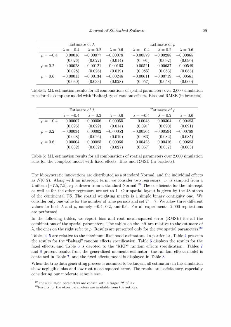
Table 4: ML estimation results for all combinations of spatial parameters over 2,000 simulationruns for the complete model with“Baltagi-type”random effects. Bias and RMSE (in brackets).
Estimate of λ Estimate of ρ
λ = −0.4 λ = 0.2 λ = 0.6
ρ = −0.4 −0.00007 −0.00056 −0.00055(0.026) (0.022) (0.014)
ρ = 0.2 −0.00034 0.00002 −0.00053(0.028) (0.026) (0.019)
ρ = 0.6 0.00004 −0.00085 −0.00066(0.032) (0.032) (0.027)
λ = −0.4 λ = 0.2 λ = 0.6
−0.0043 −0.00304 −0.00483(0.091) (0.090) (0.091)
−0.00564 −0.00594 −0.00789(0.083) (0.082) (0.085)
−0.00423 −0.00416 −0.00683(0.057) (0.057) (0.063)
Table 5: ML estimation results for all combinations of spatial parameters over 2,000 simulationruns for the complete model with fixed effects. Bias and RMSE (in brackets).
The idiosyncratic innovations are distributed as a standard Normal, and the individual effectsas N(0, 2). Along with an intercept term, we consider two regressors: x1 is sampled from aUniform [−7.5, 7.5], x2 is drawn from a standard Normal.19 The coefficients for the interceptas well as for the other regressors are set to 1. Our spatial layout is given by the 48 statesof the continental US. The spatial weighting matrix is a simple binary contiguity one. Weconsider only one value for the number of time periods and set T = 7. We allow three differentvalues for both λ and ρ, namely −0.4, 0.2, and 0.6. For all experiments, 2,000 replicationsare performed.
In the following tables, we report bias and root mean-squared error (RMSE) for all thecombinations of the spatial parameters. The tables on the left are relative to the estimate ofλ, the ones on the right refer to ρ. Results are presented only for the two spatial parameters.20
Tables 4–5 are relative to the maximum likelihood estimators. In particular, Table 4 presentsthe results for the “Baltagi” random effects specification, Table 5 displays the results for thefixed effects, and Table 6 is devoted to the “KKP” random effects specification. Tables 7and 8 present results from the generalized moments estimator: the random effects model iscontained in Table 7, and the fixed effects model is displayed in Table 8.
When the true data generating process is assumed to be known, all estimators in the simulationshow negligible bias and low root mean squared error. The results are satisfactory, especiallyconsidering our moderate sample size.
19The simulation parameters are chosen with a target R2 of 0.7.20Results for the other parameters are available from the authors.
30 splm: Spatial Panel Data Models in R
Estimate of λ Estimate of ρ
λ = −0.4 λ = 0.2 λ = 0.6
ρ = −0.4 −0.00028 −0.00053 −0.00043(0.027) (0.022) (0.014)
ρ = 0.2 0.00159 −0.00089 −0.00079(0.027) (0.026) (0.018)
ρ = 0.6 0.00143 0.00152 −0.00149(0.030) (0.034) (0.027)
λ = −0.4 λ = 0.2 λ = 0.6
−0.00516 −0.00934 −0.00857(0.083) (0.083) (0.084)
−0.01408 −0.01342 −0.01276(0.079) (0.081) (0.077)−0.0091 −0.01109 −0.01091(0.054) (0.055) (0.060)
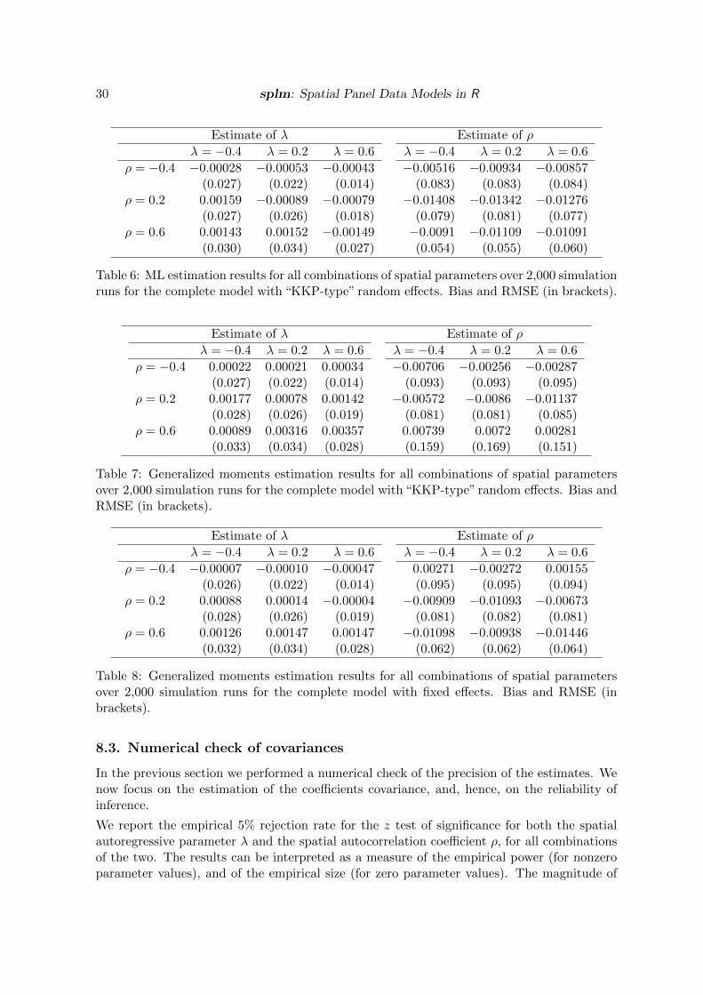
Table 6: ML estimation results for all combinations of spatial parameters over 2,000 simulationruns for the complete model with “KKP-type” random effects. Bias and RMSE (in brackets).
Estimate of λ Estimate of ρ
λ = −0.4 λ = 0.2 λ = 0.6
ρ = −0.4 0.00022 0.00021 0.00034(0.027) (0.022) (0.014)
ρ = 0.2 0.00177 0.00078 0.00142(0.028) (0.026) (0.019)
ρ = 0.6 0.00089 0.00316 0.00357(0.033) (0.034) (0.028)
λ = −0.4 λ = 0.2 λ = 0.6
−0.00706 −0.00256 −0.00287(0.093) (0.093) (0.095)
−0.00572 −0.0086 −0.01137(0.081) (0.081) (0.085)0.00739 0.0072 0.00281(0.159) (0.169) (0.151)
Table 7: Generalized moments estimation results for all combinations of spatial parametersover 2,000 simulation runs for the complete model with “KKP-type” random effects. Bias andRMSE (in brackets).
Estimate of λ Estimate of ρ
λ = −0.4 λ = 0.2 λ = 0.6
ρ = −0.4 −0.00007 −0.00010 −0.00047(0.026) (0.022) (0.014)
ρ = 0.2 0.00088 0.00014 −0.00004(0.028) (0.026) (0.019)
ρ = 0.6 0.00126 0.00147 0.00147(0.032) (0.034) (0.028)
λ = −0.4 λ = 0.2 λ = 0.6
0.00271 −0.00272 0.00155(0.095) (0.095) (0.094)
−0.00909 −0.01093 −0.00673(0.081) (0.082) (0.081)
−0.01098 −0.00938 −0.01446(0.062) (0.062) (0.064)
Table 8: Generalized moments estimation results for all combinations of spatial parametersover 2,000 simulation runs for the complete model with fixed effects. Bias and RMSE (inbrackets).
8.3. Numerical check of covariances
In the previous section we performed a numerical check of the precision of the estimates. Wenow focus on the estimation of the coefficients covariance, and, hence, on the reliability ofinference.
We report the empirical 5% rejection rate for the z test of significance for both the spatialautoregressive parameter λ and the spatial autocorrelation coefficient ρ, for all combinationsof the two. The results can be interpreted as a measure of the empirical power (for nonzeroparameter values), and of the empirical size (for zero parameter values). The magnitude of

Journal of Statistical Software 31
RE (B) ML, test λ = 0 RE (B) ML, test of ρ = 0
λ = −0.2 λ = 0 λ = 0.2
ρ = −0.2 1.000 0.056 1.000ρ = 0 1.000 0.069 1.000ρ = 0.2 1.000 0.055 1.000
λ = −0.2 λ = 0 λ = 0.2
ρ = −0.2 0.628 0.610 0.627ρ = 0 0.065 0.068 0.060ρ = 0.2 0.663 0.662 0.663
RE (KKP) ML, test λ = 0 RE (KKP) ML, test of ρ = 0
λ = −0.2 λ = 0 λ = 0.2
ρ = −0.2 1.000 0.052 1.000ρ = 0 0.999 0.065 1.000ρ = 0.2 1.000 0.059 1.000
λ = −0.2 λ = 0 λ = 0.2
ρ = −0.2 0.680 0.708 0.686ρ = 0 0.059 0.067 0.056ρ = 0.2 0.696 0.684 0.686
FE ML, test λ = 0 FE ML, test of ρ = 0
λ = −0.2 λ = 0 λ = 0.2
ρ = −0.2 1.000 0.076 1.000ρ = 0 1.000 0.099 1.000ρ = 0.2 1.000 0.067 1.000
λ = −0.2 λ = 0 λ = 0.2
ρ = −0.2 0.676 0.674 0.670ρ = 0 0.083 0.087 0.080ρ = 0.2 0.709 0.725 0.708
RE GM, test λ = 0
λ = −0.2 λ = 0 λ = 0.2
ρ = −0.2 1.000 0.056 1.000ρ = 0 1.000 0.058 1.000ρ = 0.2 1.000 0.048 1.000
FE GM, test λ = 0
λ = −0.2 λ = 0 λ = 0.2
ρ = −0.2 1.000 0.061 1.000ρ = 0 1.000 0.050 1.000ρ = 0.2 1.000 0.056 1.000
Table 9: Evaluation of covariance estimates: low correlation scenario. Empirical 5% rejectionrates of significance z tests for λ (left column) and ρ (right column) for all combinations ofspatial parameters in (−0.2, 0, 0.2). Rejection rates are a measure of empirical size where theparameter is set to zero, of empirical power elsewhere.
the deviation from the nominal size is assessed using the outcome of the test as a samplefrom a binomial variate with probability equal to the nominal size and number of draws equalto the sample size so that the standard error is
√0.05× 0.95/2000 and the 95% confidence
interval is approximately 0.04− 0.06.
Table 9 reports the empirical rejection rates for all nine combinations of λ = (−0.2, 0, 0.2)and ρ = (−0.2, 0, 0.2).21 The low levels of spatial correlation are chosen in order to checkpower against weak spatial dependence.
In Table 10 we report the same measures for a more clear-cut situation where the values of the
21 In both scenarios, in one simulation run of the combination λ = 0, ρ = 0 both the RE (B) and the FEmaximum likelihood estimators returned a singular matrix error: both these results were discarded and inthese two cases the report is based on 1999 out of 2000 runs.
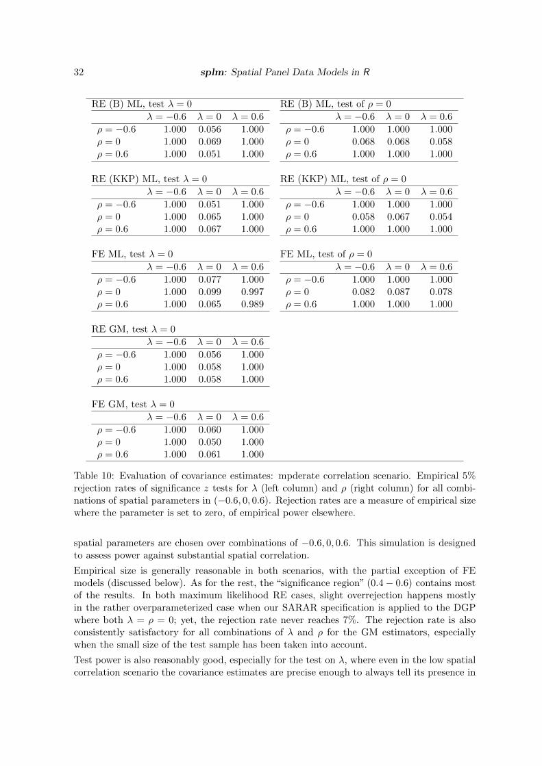
32 splm: Spatial Panel Data Models in R
RE (B) ML, test λ = 0 RE (B) ML, test of ρ = 0
λ = −0.6 λ = 0 λ = 0.6
ρ = −0.6 1.000 0.056 1.000ρ = 0 1.000 0.069 1.000ρ = 0.6 1.000 0.051 1.000
λ = −0.6 λ = 0 λ = 0.6
ρ = −0.6 1.000 1.000 1.000ρ = 0 0.068 0.068 0.058ρ = 0.6 1.000 1.000 1.000
RE (KKP) ML, test λ = 0 RE (KKP) ML, test of ρ = 0
λ = −0.6 λ = 0 λ = 0.6
ρ = −0.6 1.000 0.051 1.000ρ = 0 1.000 0.065 1.000ρ = 0.6 1.000 0.067 1.000
λ = −0.6 λ = 0 λ = 0.6
ρ = −0.6 1.000 1.000 1.000ρ = 0 0.058 0.067 0.054ρ = 0.6 1.000 1.000 1.000
FE ML, test λ = 0 FE ML, test of ρ = 0
λ = −0.6 λ = 0 λ = 0.6
ρ = −0.6 1.000 0.077 1.000ρ = 0 1.000 0.099 0.997ρ = 0.6 1.000 0.065 0.989
λ = −0.6 λ = 0 λ = 0.6
ρ = −0.6 1.000 1.000 1.000ρ = 0 0.082 0.087 0.078ρ = 0.6 1.000 1.000 1.000
RE GM, test λ = 0
λ = −0.6 λ = 0 λ = 0.6
ρ = −0.6 1.000 0.056 1.000ρ = 0 1.000 0.058 1.000ρ = 0.6 1.000 0.058 1.000
FE GM, test λ = 0
λ = −0.6 λ = 0 λ = 0.6
ρ = −0.6 1.000 0.060 1.000ρ = 0 1.000 0.050 1.000ρ = 0.6 1.000 0.061 1.000
Table 10: Evaluation of covariance estimates: mpderate correlation scenario. Empirical 5%rejection rates of significance z tests for λ (left column) and ρ (right column) for all combi-nations of spatial parameters in (−0.6, 0, 0.6). Rejection rates are a measure of empirical sizewhere the parameter is set to zero, of empirical power elsewhere.
spatial parameters are chosen over combinations of −0.6, 0, 0.6. This simulation is designedto assess power against substantial spatial correlation.
Empirical size is generally reasonable in both scenarios, with the partial exception of FEmodels (discussed below). As for the rest, the “significance region” (0.4− 0.6) contains mostof the results. In both maximum likelihood RE cases, slight overrejection happens mostlyin the rather overparameterized case when our SARAR specification is applied to the DGPwhere both λ = ρ = 0; yet, the rejection rate never reaches 7%. The rejection rate is alsoconsistently satisfactory for all combinations of λ and ρ for the GM estimators, especiallywhen the small size of the test sample has been taken into account.
Test power is also reasonably good, especially for the test on λ, where even in the low spatialcorrelation scenario the covariance estimates are precise enough to always tell its presence in
Journal of Statistical Software 33
any of the models considered. The test on ρ is not applicable to the GM models, which donot allow estimating the covariance of this parameter. As for the ML estimators, in the lowspatial correlation scenario, estimates of the power of the test are all close to 70%. When thelevel of spatial correlation is higher, the power approaches one.
The FE case deserves special attention. Some of the rejection rates (8%,) are well above theupper limit of the“significance region”. This result might at first be considered a sign of lack ofprecision of the numerical Hessian approximation used in the FE SARAR estimator. However,the same evidence is confirmed for the FE SAR and SEM estimators, which implement theanalytical expression of the parameter covariance. We believe that this result might be due tothe serial correlation induced in the residuals by the demeaning transformation. We performedsimulation experiments that seem to confirm our hypothesis. From those experiments, theresults indicate that the overrejecting behavior is more serious for small T (i.e., T = 3), withrejection rates over 12%, and disappears when T is large (i.e., T = 25). This seems thereforea methodological issue that merits further research, rather than a software implementationproblem.22 Considering that in fixed effects models the distinction between the Baltagi andKKP specifications vanishes, in light of the above result it is advisable to use the spgm functionfor estimating panels of short-to-moderate time dimension.
Covariance estimation through numerical Hessians proved reliable and precise, also whencompared with analytical expressions.23 One final issue relates to the emergence of negativeestimates for the parameters’ variance. This occurs almost exclusively when the data gen-erating process is one of the nested specifications (i.e., the value of the spatial parameter iszero), with frequencies of around 3%. Generalized moments estimators, on the other hand,are completely free from this problem.
9. Conclusions
The analysis of spatial panel data is a sub-field of econometrics that has lately been experi-encing increased methodological progress. Applied applications however are hindered by thelack of readily available software. The R environment is ideal for its development because ofthe vast infrastructure already in place for analyzing spatial data.
splm is a new package for the estimation and diagnostic testing of various spatial panel models.Supported estimation techniques include ML as well as GM. Lagrange multiplier tests alongwith a spatial version of the Hausman test are also provided.
The available techniques cover a good part of the recent developments in the spatial paneldata literature, providing easy access to estimation and tests procedures not yet available inany commercial software. Some of the functionalities in splm are also available as MATLAB orStata code, but this is the first attempt to provide a comprehensive tool within an organizedstatistical programming environment.
22The fact that time-demeaning of serially uncorrelated residuals induces serial correlation with a coefficientof −1/(T − 1) is documented in Wooldridge (2002, p. 270, Equation 10.52). The Monte Carlo simulations onwhich these considerations are based are available in the supplementary files. This problem was first recognizedby Lee and Yu (2010c). They show that the direct approach will produce inconsistent estimates of some ofthe parameters (including the variance). As already mentioned in Footnote 12, they suggest an alternativetransformation which corrects for this bias. In a future release of splm we plan to add this feature.
23Simulation results regarding the comparison between numerical and analytical Hessian-based covarianceestimation are available in the supplementary files.

34 splm: Spatial Panel Data Models in R
Whenever possible, the package is consistent with the standard conventions of the R environ-ment and in particular it borrows functionalities from spdep and plm. A new class had tobe defined for spatial panel model objects, along with methods for providing the standardsexpected by the average R user. We also achieved interoperability with generic functions, e.g.,those available in other packages such as car or lmtest.
The main developments in the foreseeable future should be directed toward the inclusionof new methodologies (e.g., Lee and Yu 2010a,c; Pesaran and Tosetti 2011, among others).Furthermore, we plan to extend the package and open it to the development of dynamicspatial panel data models. Different approaches to the implementation of the VC matrix ofthe estimators are also on our research agenda.
References
Anselin L (1988). Spatial Econometrics: Methods and Models. Kluwer Academic Publisher,Dordrecht.
Anselin L, Le Gallo J, Jayet H (2008). “Spatial Panel Econometrics.” In L Matyas, P Sevestre(eds.), The Econometrics of Panel Data – Fundamentals and Recent Developments in The-ory and Practice, pp. 624–660. Springer-Verlag.
Baltagi BH (1981). “Simultaneous Equations with Error Components.” Journal of Economet-rics, 17, 21–49.
Baltagi BH (2008). Econometric Analysis of Panel Data. 4th edition. John Wiley & Sons,New York.
Baltagi BH, Egger P, Pfaffermayr M (2007a). “Estimating Models of Complex FDI: Are thereThird-Country Effects?” Journal of Econometrics, 140, 260–281.
Baltagi BH, Egger P, Pfaffermayr M (2009). “A Generalized Spatial Panel Data Model withRandom Effects.” Working Paper 113, Center for Policy Research, Syracuse University.URL http://EconPapers.RePEc.org/RePEc:max:cprwps:113.
Baltagi BH, Griffin JM (2001). “The Econometrics of Rational Addiction.”Journal of Businessand Economic Statistics, 19(4), 449–454.
Baltagi BH, Liu L (2008). “Testing for Random Effects and Spatial Lag Dependence in PanelData Models.” Statistics and Probability Letters, 78, 3304–3306.
Baltagi BH, Liu L (2011). “Instrumental Variable Estimation of a Spatial AutoregressivePanel Model with Random Effects.” Economics Letters, 111, 135–137.
Baltagi BH, Song SH, Jung BC, Koh W (2007b). “Testing for Serial Correlation, SpatialAutocorrelation and Random Effects Using Panel Data.” Journal of Econometrics, 140(1),5–51.
Baltagi BH, Song SH, Koh W (2003). “Testing Panel Data Regression Models with SpatialError Correlation.” Journal of Econometrics, 117, 123–150.

Journal of Statistical Software 35
Bates D, Machler M (2012). Matrix: Sparse and Dense Matrix Classes and Methods. R pack-age version 1.0-4, URL http://CRAN.R-project.org/package=Matrix.
Bivand RS (2001). “More on Spatial Data Analysis.” R News, 1(3), 13–17. URL http:
//CRAN.R-project.org/doc/Rnews/.
Bivand RS (2002). “Spatial Econometrics Functions in R: Classes and Methods.” Journal ofGeographical Systems, 4, 405–421.
Bivand RS (2006). “Implementing Spatial Data Analysis Software Tools in R.” GeographicalAnalysis, 38(1), 23–40.
Bivand RS (2010). “Computing the Jacobian in Spatial Models: An Applied Survey.” Tech-nical Report 20/2010, Norwegian School of Economics and Business Administration. URLhttp://EconPapers.RePEc.org/RePEc:hhs:nhheco:2010_020.
Bivand RS (2011). spdep: Spatial Dependence: Weighting Schemes, Statistics and Models.R package version 0.5-43, URL http://CRAN.R-project.org/package=spdep.
Bivand RS, Gebhardt A (2000). “Implementing Functions for Spatial Statistical AnalysisUsing the R Language.” Journal of Geographical Systems, 2, 307–312.
Bivand RS, Portnov BA (2004). “Exploring Spatial Data Analysis Techniques Using R: TheCase of Observations with No Neighbors.” In L Anselin, RJGM Florax, SJ Rey (eds.),Advances in Spatial Econometrics: Methodology, Tools and Applications, pp. 121–142.Springer-Verlag.
Breusch TS, Pagan AR (1980). “The Lagrange Multiplier Test and Its Applications to ModelSpecification in Econometrics.” Review of Economic Studies, 47, 239–253.
Croissant Y (2011). Ecdat: Data Sets for Econometrics. R package version 0.1-6.1, URLhttp://CRAN.R-project.org/package=Ecdat.
Croissant Y, Millo G (2008). “Panel Data Econometrics in R: The plm Package.” Journal ofStatistical Software, 27(2), 1–43. URL http://www.jstatsoft.org/v27/i02/.
Debarsy N, Ertur C (2010). “Testing for Spatial Autocorrelation in a Fixed Effects PanelData Model.” Regional Science and Urban Economics, 40, 453–470.
Drukker DM, Peng H, Prucha IR, Raciborski R (2011a). “Creating and Managing Spatial-Weighting Matrices Using the spmat Command.” Technical report. URL http://econweb.
umd.edu/~prucha/Papers/WP_spmat_2011.pdf.
Drukker DM, Peng H, Prucha IR, Raciborski R (2012). sppack: Stata Module for Cross-Section Spatial-Autoregressive Models. Version 2012-01-25, URL http://EconPapers.
RePEc.org/RePEc:boc:bocode:s457245.
Drukker DM, Prucha IR, Raciborski R (2011b). “A Command for Estimating Spatial-Autoregressive Models with Spatial-Autoregressive Disturbances and Additional Endoge-nous Variables.” Technical report. URL http://econweb.umd.edu/~prucha/Papers/WP_
spivreg_2011.pdf.
36 splm: Spatial Panel Data Models in R
Drukker DM, Prucha IR, Raciborski R (2011c). “Maximum-Likelihood and Generalized Spa-tial Two-Stage Least-Squares Estimators for a Spatial-Autoregressive Model with Spatial-Autoregressive Disturbances.” Technical report. URL http://econweb.umd.edu/~prucha/
Papers/WP_spreg_2011.pdf.
Elhorst JP (2003). “Specification and Estimation of Spatial Panel Data Models.” InternationalRegional Sciences Review, 26(3), 244–268.
Elhorst JP (2008). “Serial and Spatial Error Correlation.” Economics Letters, 100, 422–424.
Elhorst JP (2009). “Spatial Panel Data Models.” In MM Fischer, A Getis (eds.), Handbookof Applied Spatial Analysis. Springer-Verlag.
Elhorst JP (2010). “Dynamic Panels with Endogenous Interactions Effects when T Is Small.”Regional Science and Urban Economics, 40, 272–282.
Elhorst JP, Freret S (2009). “Yardstick Competition among Local Governments: FrenchEvidence Using a Two-Regimes Spatial Panel Data Model.” Journal of Regional Science,49, 931–951.
Elhorst JP, Piras G, Arbia G (2010). “Growth and Convergence in a Multi-Regional Modelwith Space-Time Dynamics.” Geographical Analysis, 42, 338–355.
Elhorst P (2011). MATLAB Software to Estimate Spatial Panels. Version 2011-04-11, URLhttp://www.regroningen.nl/elhorst/software.shtml.
Fox J, Weisberg S (2010). An R Companion to Applied Regression. 2nd edition. Sage Publi-cations, Thousand Oaks.
Hausman JA (1978). “Specification Tests in Econometrics.” Econometrica, 46, 1251–71.
Kapoor M, Kelejian HH, Prucha IR (2007). “Panel Data Model with Spatially CorrelatedError Components.” Journal of Econometrics, 140(1), 97–130. TSP and Stata softwareavailable at http://econweb.umd.edu/~prucha/Research_Prog3.htm.
Kelejian HH, Prucha IR (1999). “A Generalized Moments Estimator for the AutoregressiveParameter in a Spatial Model.” International Economic Review, 40(2), 509–533.
Lee LF, Yu J (2010a). “A Spatial Dynamic Panel Data Model with both Time and IndividualFixed Effects.” Econometric Theory, 26, 564–597.
Lee LF, Yu J (2010b). “A Unified Transformation Approach to the Estimation of SpatialDynamic Panel Data Models: Stability, Spatial Cointegration and Explosive Roots.” InA Ullah, DEA Giles (eds.), Handbook of Empirical Economics and Finance, pp. 397–434.Chapman & Hall/CRC.
Lee LF, Yu J (2010c). “Estimation of Spatial Autoregressive Panel Data Models with FixedEffects.” Journal of Econometrics, 154, 165–185.
Lee LF, Yu J (2010d). “Some Recent Development in Spatial Panel Data Models.” RegionalScience and Urban Economics, 40, 255–271.

Journal of Statistical Software 37
LeSage JP (1999). Applied Econometrics Using MATLAB. URL http://www.
spatial-econometrics.com/.
LeSage JP, Pace KR (2009). Introduction to Spatial Econometrics. Chapman & Hall/CRC,Boca Raton.
Munnell AH (1990). “Why Has Productivity Growth Declined? Productivity and PublicInvestment.” New England Economic Review, 1990, 3–22.
Mutl J (2006). Dynamic Panel Data Models with Spatially Autocorrelated Disturbances. Ph.D.thesis, University of Maryland, College Park.
Mutl J, Pfaffermayr M (2011). “The Hausman Test in a Cliff and Ord Panel Model.” Econo-metrics Journal, 14, 48–76.
Pesaran HM, Tosetti E (2011). “Large Panels with Common Factors and Spatial Correlations.”Journal of Econometrics, 161(2), 182 –202.
Piras G (2010). “sphet: Spatial Models with Heteroskedastic Innovations in R.” Journal ofStatistical Software, 35(1), 1–21. URL http://www.jstatsoft.org/v35/i01/.
Piras G (2011). “Estimation of Random Effects Spatial Panel Data Models: Some AdditionalEvidence.” Unpublished Manuscript.
R Development Core Team (2012). R: A Language and Environment for Statistical Computing.R Foundation for Statistical Computing, Vienna, Austria. ISBN 3-900051-07-0, URL http:
//www.R-project.org/.
StataCorp (2007). Stata Statistical Software: Release 10. StataCorp LP, College Station, TX.URL http://www.stata.com/.
The MathWorks, Inc (2010). MATLAB – The Language of Technical Computing, Ver-sion 7.10.0. Natick, Massachusetts. URL http://www.mathworks.com/products/
matlab/.
Wooldridge JM (2002). Econometric Analysis of Cross-Section and Panel Data. MIT Press.
Yu J, de Jong R, Lee LF (2008). “Quasi Maximum Likelihood Estimators for Spatial DynamicPanel Data with Fixed Effects when both n and T Are Large.” Journal of Econometrics,146, 118–134.
Yu J, Lee LF (2010). “Estimation of Unit Root Spatial Dynamic Panel Data Models.” Econo-metric Theory, 26, 1332–1362.
Zeileis A, Hothorn T (2002). “Diagnostic Checking in Regression Relationships.” R News,2(3), 7–10. URL http://CRAN.R-project.org/doc/Rnews/.
Affiliation:
Giovanni MilloResearch & Development DepartmentGenerali SpA

38 splm: Spatial Panel Data Models in R
Via Machiavelli 334131 Trieste, ItalyTelephone: +39/040/671184Fax: +39/040/671160E-mail: [email protected]
Gianfranco PirasRegional Research InstituteWest Virginia University886 Chestnut Ridge RoadP.O. Box 6825Morgantown, WV 26506-6825, United States of AmericaE-mail: [email protected]
Journal of Statistical Software http://www.jstatsoft.org/
published by the American Statistical Association http://www.amstat.org/
Volume 47, Issue 1 Submitted: 2009-11-18April 2012 Accepted: 2012-04-05