Splittings, coalescence, bunch and snake patterns in the 3D …mezentsv/papers/PD-v151-p175.pdf · Splittings, coalescence, bunch and snake patterns in the 3D nonlinear Schrödinger

Physica D 151 (2001) 175–198

Splittings, coalescence, bunch and snake patterns in the 3Dnonlinear Schrödinger equation with anisotropic dispersion

K. Germaschewski a, R. Grauer a, L. Bergé b, V.K. Mezentsev c,d, J. Juul Rasmussen e,∗a Institute for Theoretical Physics I, Heinrich-Heine-Universität Düsseldorf, 40225 Düsseldorf, Germany

b Commissariat à l’Énergie Atomique, CEA-DAM/Ile-de-France, BP 12, 91680 Bruyères-le-Châtel, Francec Photonics Research Group, Aston University, Aston Triangle B4 7ET, Birmingham, UK

d Institute of Automation and Electrometry, 630090 Novosibirsk, Russiae Risø National Laboratory, Optics and Fluid Dynamics Department, OFD-128, P.O. Box 49,

DK-4000 Roskilde, Denmark

Received 19 July 2000; accepted 21 November 2000Communicated by A.C. Scott

Abstract

The self-focusing and splitting mechanisms of waves governed by the cubic nonlinear Schrödinger equation with anisotropicdispersion are investigated numerically by means of an adaptive mesh refinement code. Wave-packets having a power farabove the self-focusing threshold undergo a transversal compression and are shown to split into two symmetric peaks. Thesepeaks can sequentially decay into smaller-scale structures developing near the front edge of a shock, as long as their individualpower remains above threshold, until the final dispersion of the wave. Their phase and amplitude dynamics are detailed andcompared with those characterizing collapsing objects with no anisotropic dispersion. Their ability to mutually coalesceis also analyzed and modeled from the interaction of Gaussian components. Next, bunch-type and snake-type instabilities,which result from periodic modulations driven by even and odd localized modes, are studied. The influence of the initialwave amplitude, the amplitude and wavenumber of the perturbations on the interplay of snake and bunch patterns are finallydiscussed. © 2001 Elsevier Science B.V. All rights reserved.

PACS: 42.65.Jx; 42.25.Bs; 03.40.Kf

Keywords: Nonlinear Schrödinger equation; Anisotropic dispersion; Bunch- and snake-type patterns; Splitting; Coalescence

1. Introduction

The self-focusing of wave-packets in nonlinear dispersive media is generally described by the nonlinearSchrödinger (NLS) equation, which reads in normalized form

i∂tE +�⊥E + s∂2z E + |E|2E = 0, (1)

where E(x, y, z, t) represents the scalar, slowly varying envelope of a wave with isotropic (s > 0) or anisotropic(s < 0) dispersion. For localized waveforms, for which E and its derivatives all vanish at boundaries, Eq. (1) is

∗ Corresponding author. Tel.: +45-4677-4537; fax: +45-4677-4565.E-mail address: [email protected] (J. Juul Rasmussen).

0167-2789/01/$ – see front matter © 2001 Elsevier Science B.V. All rights reserved.PII: S0 1 6 7 -2 7 89 (01 )00144 -0

176 K. Germaschewski et al. / Physica D 151 (2001) 175–198

conservative and preserves the Hamiltonian

H =∫

{| �∇⊥E|2 + s|Ez|2 − 12 |E|4} d�r dz, (2)

together with the total “power” or “mass”

N ≡∫

|E|2 d�r dz. (3)

In the context of plasma physics, Eq. (1) applies to the description of nonlinear waves with an anisotropic dispersion,i.e., with a dispersion law ω(�k) such that the second-order derivatives ∂2ω/∂k2

x, ∂2ω/∂k2

y and ∂2ω/∂k2z differ in

sign. Among those, we mention lower-hybrid, ion-cyclotron waves [1] and whistlers or oblique plasma waves inmagnetized plasmas, for which the wavevector surface near the point of the central wavevector has a negativecurvature [2]. In the scope of nonlinear optics, the variable t often refers to the longitudinal length along the beampropagation axis, whereas z corresponds to a retarded time variable t ′ = t − z/ω′ (ω′ ≡ ∂ω/∂k). The term s∂2

z E

in Eq. (1) then reflects the “temporal” dispersion related to the group velocity dispersion (GVD) with coefficients ∼ ∂2k/∂ω2|ω0 [3].

The dynamics of E for isotropic dispersion s > 0 is rather well understood [4,5]. Briefly speaking, a localizedwave-packet undergoes a 3D collapse when H < 0. In contrast, for the anisotropic case, the detailed evolutionremains partly unclear. The main unresolved points are: Can the formation of a collapse-like singularity appearin the solution E for some initial conditions? How does the negative dispersion term affect the characteristicsof the self-focusing in the transverse plane and, in connection with this, what is the ultimate fate of a transver-sally self-contracting wave-packet? Various theoretical, numerical and experimental investigations suggest thatcollapse should not occur as a point-singularity when s < 0. Instead, with anisotropic dispersion, the wave-packetself-contracts in the transverse plane, but it expands in the longitudinal direction and subsequently splits into twopeaks [6–9,40]. The resulting peaks may promote further splittings if their power is sufficiently strong [10–13]. Thedynamics of this process is, however, not yet completely understood and there exist some controversial opinions[14–16]. From the numerical point of view, the main limiting factor in describing the detailed wave dynamics hasbeen the obtainable resolution in the solutions of Eq. (1), when applying conventional numerical schemes. Conse-quently, only numerical attempts dealing with limited powers, for which one splitting event and the formation oftwo cells have clearly been detected, seem to have been sufficiently resolved to yield trustworthy results (see, e.g.[17–20]). For higher power levels, even in the most recent numerical studies that were sometimes supported bysuccessively refined resolutions, different self-contradictory scenarios have been emphasized, from the total absenceof secondary splitting events [14,15] to the formation of extra cells after the first peaks moved to the boundaries ofthe numerical box [18]. Therefore, we find it necessary to detail more the nonlinear evolution of wave-packets inmedia with anisotropic dispersion by performing precise numerical simulations of the (3 + 1)-dimensional cubicnonlinear Schrödinger equation (1) with s < 0. To this aim, we have employed a numerical algorithm with very finespatial and temporal resolutions based on an adaptive mesh refinement method. This allows us to follow accuratelythe evolution of extremely narrow structures having amplitudes exceeding the initial wave amplitude by severalorders of magnitude.

First, we investigate the evolution of localized Gaussian waves. When they possess a peak power well above theself-focusing threshold, these undergo a transversal compression. However, at least for all numerically accessiblecases supporting a reliable resolution, they do not collapse to a singularity. Instead, they rather split into twosymmetric packets, each of which may sequentially produce small-scale structures as long as their individual powerremains above threshold. Such secondary structures generically emerge as lower-amplitude ripples forming in thefinal dispersion regime. These results are discussed in terms of the existing theory, which we briefly recall. Second,

K. Germaschewski et al. / Physica D 151 (2001) 175–198 177

we consider the evolution of modulational instabilities of waveguide beams along the z-axis. We study both theevolution of even perturbations, leading to the so-called bunch modes, and odd perturbations, producing the so-calledsnake modes. Generally, when perturbations include both even and odd modes, the waveguide begins being distortedby a snake dynamics, but it finally decays into bunches. These results agree with theoretical predictions emphasizedbelow. The paper is organized as follows. In Section 2, we review theoretical results. Section 3 describes theadaptive mesh algorithm constructed for solving Eq. (1). Then, in Section 4, we describe the results of the numericalsolutions for nonlinear waves with anisotropic dispersion and emphasize their ability to split into multiple small-scalestructures. Section 5 is devoted to the formation and competition of bunches and snakes issued from the modulationalinstability of Gaussian wave solutions to Eq. (1). Finally, Section 6 contains our concluding remarks.

2. Review of theoretical results

We review basic theoretical results concerning the dynamics of solutions to the 3D NLS equation with anisotropicdispersion. In what follows, we term the full solution E as “wave”, “wave-packet” or “beam”, while the first twostructures resulting from a primary splitting are conventionally called “peaks” or “pulses”. The substructures formedfrom the latter will be called “cells” or “ripples”. Also, we will indistinguishably employ the wording “power” or“mass” for denoting the L2 norm (3).

As a starting point before discussing the anisotropic dynamics, we recall the self-focusing (collapse) propertiesof solutions to the 2D Eq. (1) with s = 0.

2.1. Critical collapse

Non-stationary solutions of Eq. (1) with s = 0 are subject to collapse, which leads the amplitude |E| to blowup in finite time. For initial wave functions E(�r, t = 0) ≡ E0(�r) formulated in the Sobolev space H 1, the L2

norm of the solution is conserved with ‖E‖22 = ‖E0‖2

2 and E exists as long as it keeps a finite H 1 norm ‖E‖H 1 =(‖E‖2

2 + ‖�∇E‖22)

1/2 < +∞, where ‖f ‖p ≡ (∫ |f |p d�r)1/p. A blow-up is then defined by the existence of a finite

time t0 < +∞, such that ‖E‖H 1 → +∞ for t → t0, which implies that the gradient norm ‖ �∇E‖22 and thereby

max|E(�r, t)| diverge in the same limit [21,22]. This singular dynamics follows from the vanishing of the so-calledvirial integral

I (t) ≡ ‖�rE‖22 =

∫r2|E|2 d�r → 0 as t → t∗0 < +∞, t∗0 ≥ t0, (4)

where the instant t∗0 , at which I (t = t∗0 ) is zero, is generally larger than the time t0, at which the blow-up singularityactually occurs. Here, I (t) is a measure of the square width of the wave-packet. Its evolution is governed by∂2t I (t) = 8H , which shows that a given initial waveform with H < 0 inevitably collapses into a point-singularity.

In addition, the inequality [4]

‖E‖22 ≤ ‖�∇E‖2‖�rE‖2 (5)

displays evidence that non-trivial solutions E have their gradient norm tending to infinity as t → t∗0 , so that thesolution cannot globally survive inH 1. A necessary condition for the blow-up to take place is ‖E‖2

2 > Nc � 11.68.The critical mass, Nc, is the norm calculated on the stationary solution, E(r, t) = φ0(r) eit [23], where φ0 is thepositive (nodeless), radially symmetric ground-state solution of −φ0 + r−1∂rr∂rφ0 + φ3

0 = 0.In radial geometry, a collapsing field is self-similarly modeled as

E(r, t) = 1

R(t)φ(ξ, τ ) exp

(iτ − iβξ2

4

), (6)


where β is a time-dependent function β(t) ≡ −RR (dot means a differentiation with respect to time), ξ ≡ r/R(t)

is the spatial coordinate rescaled with the wave radius R(t), and τ(t) is the new time variable τ(t) ≡ ∫ t0 du/R2(u).

Thus, Eq. (6) describes the divergence of the wave when R(t) → 0. By inserting the solution (6) into Eq. (1) withs = 0, we obtain the transformed NLS equation

i∂τφ +�ξφ + |φ|2φ + [ε(τ )ξ2 − 1]φ = 0 (7)

with �ξ = ξ−1∂ξ ξ∂ξ and

ε(τ ) ≡ − 14R

3R = 14 (β

2 + βτ ). (8)

To determine R(t), solutions to Eq. (7) are assumed to reach a self-similar state satisfying the limit ∂τφ → 0,while the functions ε and β converge adiabatically towards stationary values ε0 and β0 by satisfying ε � 1

4β2 with

|∂τβ| � β2. It is then convenient to divide the solution φ into two distinct contributions, namely, a core φc and atail φT:

φ(ξ, τ ) = φc(ξ, τ )+ φT(ξ, τ ), (9)

where φc corresponds to the central part of φ located at ξ < ξT. In this region, φc is close to the exact self-similarstate φ0(ξ) and it can be expressed perturbatively as a Taylor expansion

φc(ξ, ε) = φ0(ξ)+ (ε − ε0)∂φ

∂ε

∣∣∣∣ε0

+ · · · . (10)

On the other hand,φT extends in the complementary domain ξ > ξT, where the cubic nonlinearity can be disregarded.φT is then a solution of a parabolic cylinder equation, reading [5,15,24–27]

φT(ξ, ε) � C(ε)ei

√εξ2/2

ξ1+i/2√ε, |C(ε)| ∝ ε−1/4 e−π/4√ε . (11)

By inserting Eqs. (9)–(11) into the mass continuity equation for φ:∫ ξ

0∂τ |φ(ξ ′, τ )|2ξ ′ dξ ′ = −2|φ(ξ, τ )|2ξ∂ξ arg {φ(ξ, τ )}, (12)

the function ε is found to obey

∂τ ε � −2K exp

(− π

2√ε

), (13)

whereK is a positive constant. This function asymptotically tends to zero together with β, and a log–log contractionscale

R(t) = R(0)

√2π(t0 − t)

ln ln [1/(t0 − t)], (14)

thus follows, after solving β(t) = −RR and employing τ(t) � ln [1/(t0 − t)].

2.2. Self-focusing in 3D anisotropic media

For anisotropic media with negative s in Eq. (1), former studies [6–9,40] showed that the wave evolution resultsfrom the interplay between a 2D compression in the transverse plane and a stretching along the z-axis. This


competition leads to the splitting of a single wave into two smaller-scale peaks, accompanied by a simultaneouscompression of the resulting structures. In these first works, numerical simulations emphasized that initially Gaussianwaves started to split up, whenever their input transverse mass

N⊥(0) =∫ +∞

−∞

∫ +∞

−∞|E(x, y, z = 0, t = 0)|2 dx dy (15)

exceeds slightly Nc as, e.g., N⊥(0) ≥ 1.3Nc [7,8] for rather weak values of |s|. More recently [12,19], it wasobserved that splitting clearly occurred as soon as N⊥(0) > (1.4 − 1.5)Nc and the resulting pulses ultimatelydisperse as their individual transverse mass becomes below critical. Thus, negative dispersion is able to stop atransverse collapse, as shown by Luther et al. [9], who described the arrest of collapse by treating self-similarlythe term s∂2

z E as a diffusive perturbation, that damps the transverse cross-sections of the wave with highest peakpower (i.e., with the shortest focal point, t0). This analysis was applied to waves with masses close to threshold. ForN⊥(0) � Nc and s = −1, Zharova et al. [10] earlier proposed that a localized waveform initially stretched along zsequentially decays into multiple cells, which disperse at large times. This scenario was supported by a numericalintegration of Eq. (1) performed in axis-symmetric geometry.

To obtain a better understanding of this problem, Fibich and Papanicolaou [14,15] elaborated on a perturbationtheory, valid when s is small (|s| � 1) and whenN⊥ is larger than, although very close to, the collapse thresholdNc.Their procedure consists in perturbing the asymptotic state, towards which the unperturbed NLS solution convergesas t → t0, namely

Es(r, z, t) = 1

R(t, z)φ0(ξ) eiS(r,z,t), S(r, z, t) = τ(t, z)+ Rt(t, z)

4R(t, z)r2 (16)

with ξ ≡ r/R(t, z) and τ(t, z) ≡ ∫ t0 dv/R2(v, z). Here, φ0 is the radially symmetric ground state introduced in

Section 2.1 andR(t, z)denotes the radial scale function, varying with both z and t , which undergoes the modificationsinduced by s∂2

z E. This perturbation theory only applies to wavefields self-focusing with R(z, t) → 0 near a focuspoint t0, under the assumptions that s∂2

z E not only remains small compared with the other terms of Eq. (1), but italso keeps the functions β and ε in Eq. (8) small compared to unity, as the shape of E becomes closer and closer toφ0. Under these conditions, the equation for ε reads

εt + ν(ε)

R2= (f1)t

2M− 2f2

M, (17)

where ν(ε) ∼ K e−π/2√ε follows from Eq. (13), M ≡ ∫ξ2φ2

0 d�ξ ,

f1(z, t) ≡ 2sR3 Re∫

{(∂2z Es) e−iS[1 + ξ∇ξ ]φ0(ξ)} d�ξ, (18)

f2(z, t) ≡ sR2 Im∫

{E∗s (∂

2z Es)} d�ξ . (19)

In the limits e−π/2√ε � |(f1)t |/|f2| ∼ β � 1 and f2 ∼ sNcτzz, the dynamical system constituted by

ε ≡ −1

4R3R, εt � −2sNcτzz

M, τt = 1

R2, (20)

provides the evolution of the wave amplitude ∼ 1/R along z at different times. By doing so, the estimate of R(t, z)obtained from Eq. (20) restores the qualitative shape of one splitting event, with two spikes emerging symmetricallyalong z. To understand the meaning of Eq. (20), we stack the wave into transverse cross-sections over the longitudinalaxis and assume that these slices self-focus individually with the contraction scale R(t, z) = R[t0(z) − t]. Here,


t0(z) is the collapse curve in the (t, z)-plane, such that at z = z0, t0(z) attains its minimum with T0 ≡ dzt0(z0) = 0and T0 ≡ dzzt0(z0) > 0. The value of t0(z) decreases all the more as the power in the transverse slices is high. Thevariation of ε then becomes after a simple integration

ε = ε0 + γ (−T0τ + T 20 τt ), (21)

where ε0 = ε(0, z)− γ T 20 /R

2(0, z) and γ = −2sNc/M . The effect of anisotropic dispersion is thus to decrease εto negative values at the slices of highest power, and, thereby, to stop their collapse. Due to the symmetry in z, thisresults in the formation of two symmetric spikes, for a wave centered around z0 = 0.

However, the basic hypotheses |β|, ε � 1 underlying the derivation of Eqs. (17) and (20) break down as the terms∂2z E becomes non-perturbative and promotes sharp longitudinal gradients near the focal point t0. Even for waves

with a relative deviation of only 10% above the threshold Nc, Eq. (20) does not predict the dispersion of the splitpeaks, but instead a collapse-like behavior with diverging amplitudes. As checked below (see Fig. 6(d)), initial dataclose to critical with N⊥ = 1.1Nc and small |s|, spread out at large times, while the discussed perturbation theoryindicates a collapse. Therefore, by construction, this perturbative procedure cannot predict the fate of the resultingspikes for t > t0. In spite of this, arguments based on this method were given for suggesting that pulses should notproduce further splittings [14,15]. It was argued that as the numerical solution may depart from the 2D focusingdynamics, this could prevent secondary splittings. We shall see below that after the focal point t0, the solution canpersistently self-focus and still decays into small-scale cells. Thus, the aforementioned discrepancies do certainlynot forbid the solution to be capable of reforming focusing spikes at later times.

To describe the splitting phenomenon, an alternative method was proposed in [11,19,28]. First, from Eq. (1),the evolutions of the integrals giving a measure for the longitudinal and transverse square-radii of the wave werecomputed as

∂2t Iz(t) ≡ ∂2

t ‖zE‖22 = 8s2‖∂zE‖2

2 − 2s‖E‖44, (22)

∂2t I⊥(t) ≡ ∂2

t ‖rE‖22 = 8‖ �∇⊥E‖2

2 − 4‖E‖44, (23)

where ‖f ‖pp ≡ ∫ |f |p d�r dz. From these expressions and setting s = −1 for simplicity, it was demonstrated thatfor any initial data, Iz(t) not only never vanishes in finite time, but it is also always bounded from below by a finitepositive quantity. Furthermore, regarding the evolution of I⊥(t), a transverse collapse defined by I⊥ → 0 was shownto never take place in the total compression regime for which the requirements Iz < 0 and I⊥ < 0 simultaneouslyhold in the vicinity of a given instant t∗0 . For any time interval [T0, t

∗0 [ where the wave fully self-contracts, this

property indeed follows from the estimate [28]

E(t) = IzI⊥ + 4H(I⊥ − 2Iz)− 4N2 ln(I⊥)− 2N2 ln(Iz) ≤ E(T0) < +∞, (24)

such that I⊥(t) cannot vanish under the above assumptions and no singular concentration of the peak intensity,leading to an NLS collapse, is possible.

Secondly, the splitting process was described by employing a quasi-self-similar analysis involving a longitudinalsize Z(t) assumed to increase, while the transverse size R(t) decreases near a focus point t0. The quasi-self-similaranalysis is based on the two-scaled solution

E(�r, z, t) =√A

R(t)√Z(t)

φ(ξ, ζ, τ (t)) exp

{iλτ(t)+ i

RtR

4ξ2 − i

ZtZ

4ζ 2}, (25)

τ(t) ≡∫ t

0

du

R2(u), ξ ≡ r

R(t), ζ ≡ z

Z(t), (26)


where A is a constant intensity factor and λ > 0 denotes the eigenvalue attached to NLS, which assures localizedeigenstates φ vanishing at infinity. Inserting Eq. (25) into (1) leads to a self-similarly transformed equation for φ,involving the time-dependent functions

εR = 14 [a2

R + ∂τ (aR)] = − 14R

3Rtt, γ εZ = − 14R

2ZZtt (27)

with aR ≡ −RRt and γ (t) ≡ R2(t)/Z2(t). As t → t0, it can be justified that both functions (27) tend to values ofcomparable magnitude, |ε|, in the self-similar limit ∂τφ → 0 reached as τ(t) → τ(t0) = +∞. By using the rapiddecrease of γ (t) → 0, the eigenfunction φ, once appropriately renormalized, is found to obey a quasi-2D equation

i∂τ φ + ∂2ξ φ + 1

ξ∂ξ φ + [ε(ξ2 + ζ 2)− λ]φ + |φ|2φ = 0, (28)

where the rescaled z-derivatives disappear with γ (t). The variable ζ plays the role of a localizing parameter, as φ,satisfying ∂τ φ → 0, can only be localized along the ζ -axis for λ ≡ λ − εζ 2 > 0. The mass continuity relationassociated with Eq. (28), which describes the mass exchanges in the transverse plane between the inner core andasymptotic tail of the solution, finally yields

∂τ ε = −2K exp

[−π(λ− εζ 2)

2√ε

](29)

withK > 0. From Eq. (29), aR ∼ 2√ε is positive in the localizing domain ζ < ζ ∗ ≡ √

λ/ε, yielding a contractionrate R(t) close to (14), but negative in the delocalizing domain ζ > ζ ∗ for which R(t) is dispersing. This scalemust thus reach a minimum value in the vicinity of the caustics ζ ∗ �= 0, where |E|2 attains a maximum. In the limitζ → ζ ∗, Eq. (29) leads to εR ∼ −2τ < 0 as τ → +∞, forcing ultimately R(t) to disperse, not to vanish, whichforbids a self-similar transverse collapse. Instead, two symmetric spikes of the field develop around z = ±Z(t0)ζ ∗,which explains the occurrence of one splitting event. For high-power (N⊥ � Nc) wave-packets, it was conjecturedthat the wave may continue to split up into smaller cells, which result from repeating the above analysis on eachpulse isolated from its neighbor. Because this process stops when their mass is under threshold, the total numberof cells produced near the point of maximal transverse compression was empirically estimated as twice the ratioN⊥(t0)/Nc, which was found to be compatible with the number of split pulses revealed in optical experiments[12,13].

As emphasized in [20], it is actually unknown whether a finite-time collapse can occur. Also, the question of thepossibility for the two pulses formed by a primary splitting to split again is still an open issue, because very fewnumerical works that clearly confirm secondary peak formation have been performed so far. Therefore, both thesepoints will be addressed in this paper. We shall see, in particular, that although each peak may undergo sequentialdivisions, these take place near the outer edge of the pulses that develop shock dynamics and produce an asymmetryin the longitudinal distribution of the wave.

2.3. Bunches and snakes driven by modulation instabilities

Modulational instabilities develop when wave-packets, close to the stationary solution E(r, t) = φ0(r; λ) eiλt

where φ0 obeys the differential equation

−λφ0 +�⊥φ0 + φ30 = 0, λ > 0 (30)

are split or bent by periodic modulations developing along the z-axis. Here, the stability of the soliton-like stateφ0(�r; λ) is analyzed with respect to perturbations in the form [a(�r)+ ib(�r)]exp(ikz+γ t), characterized by a growth


rate γ for real localized functions a(�r), b(�r). For 1D solitons ( �∇2⊥ = ∂2

x ), Zakharov and Rubenchik [29] establishedthat, in the limit of small k, the growth rate is given by γ 2 = 4sλk2 for the so-called unstable even mode leading toa bunching-type perturbation when s > 0, and by γ 2 = − 1

3 4sλk2 for the unstable odd mode leading to a bendingwhen s < 0 (see also Refs. [30,31]). For 2D solitary waves, these two kinds of instability coexist with anisotropicdispersion, as we briefly describe in the following.

In the case of axis-symmetric solutions, for which the angular dependencies are ignored in the transverse Laplacian�⊥ = ∂2

r + (1/r)∂r , the waveguide solution φ0 can be perturbed as

E(r, z, t) = {φ0(r; λ)+ εφ1(r, z, t)}exp(iλt), (31)

where ε � 1 and the perturbation φ1 decomposes into two real normal modes (a, b), such as φ1 = [a(r) +ib(r)] eikz+γ t . Inserting (31) into Eq. (1) and linearizing the resulting equation yields the non-self-adjoint eigenvalueproblem

(L1 + µ)a = −γ b, (L0 + µ)b = γ a, (32)

where L0 = λ − ∇2⊥ − φ2

0 , L1 = λ − ∇2⊥ − 3φ2

0 and µ ≡ sk2. This spectral problem is solved analytically bydetermining the perturbations acting on marginally stable states defined for γ = 0 in the long wavelength limitk → 0. In this limit, the eigenstates of Eq. (32) form an orthogonal basis of four localized eigenvectors spanned byφ0 and ∂λφ0. Direct perturbation techniques then lead to [11,29,30]

γ 4 � 16λ2µ〈φ2

0〉〈r2φ2

0〉, (33)

yielding γ 2 ∼ λ3/2√

|s|k2 with an extremum attained around |s|k2 ∼ λ, for eigenmodes scaling as a � γ ∂λφ0, b �φ0 at leading order (γ 2 → 0). Here, φ0 and ∂λφ0 are even functions that both reach a maximum at center and decayto zero as r → +∞. This implies that the equipotentials of φ are split up for ε �= 0 into periodic bunches with theperiodicity 2π/k. So, φ0 is modulationally unstable with respect to longitudinal perturbations that break it up intoperiodic bunches in the long wavelength limit k → 0 for both signs of s. For s < 0, it was moreover shown [11]that the perturbation φ1 is responsible for a mass outflow expelled out of the bunches along z.

Nonetheless, these results only concern axis-symmetric perturbations, whose angular dependence has been disre-garded. In a more complete geometry (r, θ, z), the nature of the instability can change because of the azimuthal angleθ occurring in the transverse Laplacian operator�⊥ = ∂2

r + (1/r)∂r + (1/r2)∂2θ . In this case, non-axis-symmetric

perturbations, characterized by a phase in the form eimθ with |m| = 1, consist of odd normal modes spanned byeimθ∂rφ and eimθrφ. They also contribute to the instability of the waveguide by displacing its center and promotinga spontaneous bending in media with negative dispersion, in a way similar to the bending of 1D solitons whens < 0. The growth rate is then given in the long wavelength limit by γ 2 � −2sλk2 [29,30]. Note that for s > 0, thewaveguide is stable against bending perturbations. From the above estimates, we can thus infer that a modulationalregime favoring bunch formation should dominate for small k, since γ 2

bunch > γ 2snake as k → 0. On the other hand,

the waveguide φ0 might first undergo bending for large k > 1, if we a priori extrapolate the estimates γ 2bunch ∼ k

and γ 2snake ∼ k2 to larger wavenumbers. To clear up this point, it is worthwhile investigating the development of

each instability and to study their mutual interplay numerically, which will be done in Section 5.

3. Numerical method: the adaptive mesh refinement solver

The idea of adaptive mesh refinement is near at hand. Starting with one grid of given resolution (in most of our3D configurations we currently chose 64 × 64 × 96 mesh points), the partial differential equation (1) is solved with


an appropriate scheme summarized below. After a certain number of time steps, it is checked whether the localnumerical resolution is still sufficient on the entire grid. If it is detected that locally finer grids are needed, a firstrefinement is carried out. In order to prepare for it, the points where the error of discretization exceeds a givenvalue are marked on the grid. In addition to these grid points, adjacent ones are included. These marked pointsof insufficient numerical resolution have to be covered with rectangular grids of finer resolution as efficiently aspossible. Our algorithm for this purpose is very similar to the one used by Berger and Colella [32], and it wasdescribed in detail by Friedel et al. [33]. On the grids of the newly built level, the spatial discretization length andthe time step are reduced by a factor ρ, which is called refinement factor. The new grids are filled with data obtainedby interpolation from the preceding coarser level. On both levels, the integration advances until the resolution againbecomes locally insufficient. The rebuilding of the grid hierarchy starting with the current level and proceeding onall subsequent levels begins when the above-mentioned threshold for the error is locally exceeded, e.g., if the regionsof high field strength have moved out of the region covered with finer grids, or if local gradients have developed,such that the prescribed accuracy is not guaranteed. The points of insufficient numerical resolution are collected onall grids of each level. On the basis of the resulting list of these points, new grids are generated. After assuring thatthe newly generated grids are properly embedded in their parent grids, interpolated data are filled in. If data existedon grids of the same level before the regridding, these are substituted to the interpolated data from the parents grids.

Solving the 3D NLS equation in the outlined framework requires us to select an appropriate numerical integrationscheme. It turned out that we could achieve optimal performance by using a different scheme on the refined levelsthan on the base level, when taking into account that arbitrary mesh sizes on the refined levels occurred.

On the base level, we applied an operator-splitting method which is second-order accurate in time. By justconsidering the nonlinear part of the equation, the exact solution is known and used to advance the field in directspace. Using periodic boundary conditions, the linear part is easily integrated in Fourier space and conversionbetween direct and Fourier spaces is handled by means of a fast Fourier transform. Periodic boundary conditionsdo not impose a restriction on our problem, because the localized wave-packets vanish at the boundaries during theentire evolution in time.

On the refined meshes we apply a unitary, semi-implicit scheme of Crank–Nicholson-type, which was used by,e.g., Pietsch et al. [34]. The discretization reads

[1 − 12 i�t(Lnijk + 1

2�t(∂t |ψ |2)nijk)]ψn+1ijk = [1 + 1

2 i�t(Lnijk + 12�t(∂t |ψ |2)nijk)]ψnijk (34)

with Lnijk ≡ �⊥ + s∂2z + |ψnijk|2. To invert the operator on the left-hand side, we must solve a Helmholtz-type

equation. Since this linear operator is close to identity for small time steps�t , we employ a standard Gauss–Seidelrelaxation method with red/black ordering on each grid. In order to solve the problem globally, we perform anadditive Schwarz iteration [35] on top of the per-grid solvers.

It is important to comment on the criterion for refinement. We calculate the right-hand side of Eq. (34) basedon the actual grid spacing and twice the grid spacing. When the difference exceeds a given threshold, those meshpoints are marked under-resolved and are subject to refinement. The threshold value conditioning the refinementwas determined such that a sufficient resolution was guaranteed during the temporal evolution. The length of thetime step was dynamically adapted to ensure that at all times the Courant–Friedrich–Levy condition was met andthe iterative method converged at a prescribed minimal rate.

The implementation of the adaptive mesh refinement strategy is done in C++. Handling of the data structures isseparated from the problem under consideration. Therefore, it is relatively easy to use the code for other types ofproblems, like, e.g., the 3D incompressible Euler equations [36]. Computations were performed on an SGI Origin2000 distributed shared memory (ccNUMA) machine. Since on each grid the time stepping and the Helmholtz-typeequation can be solved independently and the number of grids supersedes the number of processors available to


us, parallelization is highly efficient. We implemented the parallelization using POSIX threads, so that the code isactually portable.

4. Splittings and coalescence of Gaussian beams

This section deals with the dynamics of wave-packets described by Eq. (1), starting from the single-hump initialcondition

E(x, y, z, t = 0) = E0 exp

(−x

2 + y2

2R20

− z2

2Z20

)(35)

with a transverse mass, N⊥(0) = πR20E

20 , well above the critical power Nc. Here, different values of the initial

amplitudeE0 comprised in the range 2.3 ≤ E0 ≤ 4 and different anisotropy ratiosR0/Z0 are considered. In Section4.1, we detail the dynamics of the wavefield amplitude |E| in space and time, together with the phase dynamics. Weobserve that the dispersion of split pulses is accompanied by the formation of secondary focusing cells. In Section4.2, we discuss the influence of the dispersion coefficient s on the splitting threshold. For weak values of s, thedecay of a split pulse into several cells is again confirmed. From this, we investigate in Section 4.3 the possibilityof promoting secondary splitting events on peaks created from the first splitting, by monitoring artificially the latterwith two initially separated Gaussians and by chirping the phase of the wave appropriately. The phenomenon ofcoalescence taking place between the two main peaks along the longitudinal axis, which acts against the formationof symmetric split pulses, is thoroughly discussed.

4.1. Evolution of high-power Gaussian wave-packets

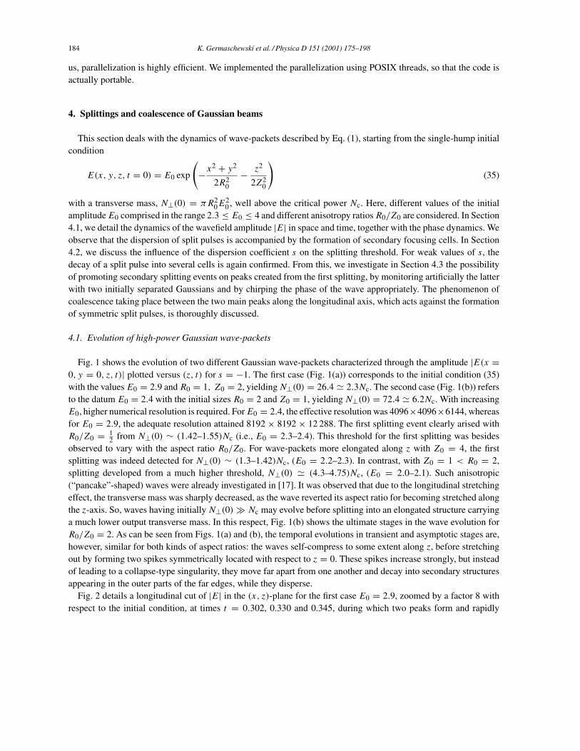
Fig. 1 shows the evolution of two different Gaussian wave-packets characterized through the amplitude |E(x =0, y = 0, z, t)| plotted versus (z, t) for s = −1. The first case (Fig. 1(a)) corresponds to the initial condition (35)with the valuesE0 = 2.9 andR0 = 1, Z0 = 2, yieldingN⊥(0) = 26.4 � 2.3Nc. The second case (Fig. 1(b)) refersto the datum E0 = 2.4 with the initial sizes R0 = 2 and Z0 = 1, yielding N⊥(0) = 72.4 � 6.2Nc. With increasingE0, higher numerical resolution is required. ForE0 = 2.4, the effective resolution was 4096×4096×6144, whereasfor E0 = 2.9, the adequate resolution attained 8192 × 8192 × 12 288. The first splitting event clearly arised withR0/Z0 = 1

2 from N⊥(0) ∼ (1.42–1.55)Nc (i.e., E0 = 2.3–2.4). This threshold for the first splitting was besidesobserved to vary with the aspect ratio R0/Z0. For wave-packets more elongated along z with Z0 = 4, the firstsplitting was indeed detected for N⊥(0) ∼ (1.3–1.42)Nc, (E0 = 2.2–2.3). In contrast, with Z0 = 1 < R0 = 2,splitting developed from a much higher threshold, N⊥(0) � (4.3–4.75)Nc, (E0 = 2.0–2.1). Such anisotropic(“pancake”-shaped) waves were already investigated in [17]. It was observed that due to the longitudinal stretchingeffect, the transverse mass was sharply decreased, as the wave reverted its aspect ratio for becoming stretched alongthe z-axis. So, waves having initially N⊥(0) � Nc may evolve before splitting into an elongated structure carryinga much lower output transverse mass. In this respect, Fig. 1(b) shows the ultimate stages in the wave evolution forR0/Z0 = 2. As can be seen from Figs. 1(a) and (b), the temporal evolutions in transient and asymptotic stages are,however, similar for both kinds of aspect ratios: the waves self-compress to some extent along z, before stretchingout by forming two spikes symmetrically located with respect to z = 0. These spikes increase strongly, but insteadof leading to a collapse-type singularity, they move far apart from one another and decay into secondary structuresappearing in the outer parts of the far edges, while they disperse.

Fig. 2 details a longitudinal cut of |E| in the (x, z)-plane for the first case E0 = 2.9, zoomed by a factor 8 withrespect to the initial condition, at times t = 0.302, 0.330 and 0.345, during which two peaks form and rapidly


Fig. 1. Wave amplitude |E| versus (z, t) for (a) E0 = 2.9 with R0 = 1 and Z0 = 2 (top) and (b) E0 = 2.4 with R0 = 2 and Z0 = 1 (bottom),in the time interval involving splitting events. Late times are displayed in front.

disperse. Here, the wave transversally shrinks and is longitudinally stretched. This results in two peaks, whichspread out by generating secondary ripples developing with smaller amplitude outside the central spikes.

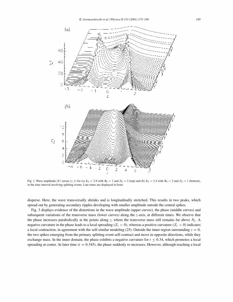
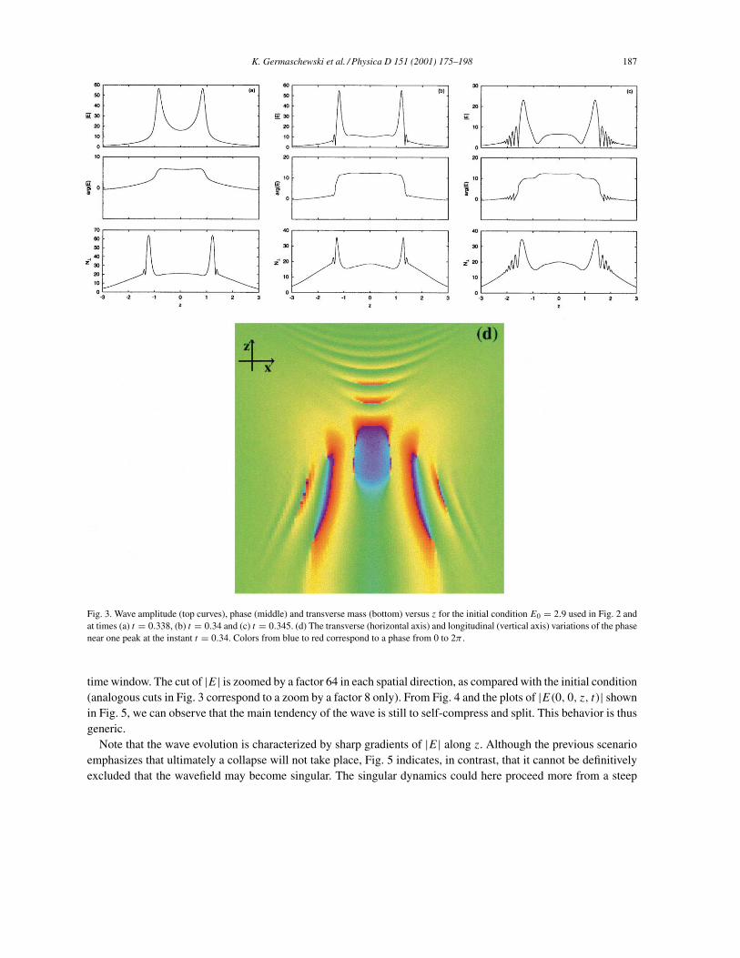
Fig. 3 displays evidence of the distortions in the wave amplitude (upper curves), the phase (middle curves) andsubsequent variations of the transverse mass (lower curves) along the z-axis, at different times. We observe thatthe phase increases parabolically at the points along z, where the transverse mass still remains far above Nc. Anegative curvature in the phase leads to a local spreading (Zt > 0), whereas a positive curvature (Zt < 0) indicatesa local contraction, in agreement with the self-similar modeling (25). Outside the inner region surrounding z = 0,the two spikes emerging from the primary splitting event self-contract and move in opposite directions, while theyexchange mass. In the inner domain, the phase exhibits a negative curvature for t ≤ 0.34, which promotes a localspreading at center. At later time (t = 0.345), the phase suddenly re-increases. However, although reaching a local


Fig. 2. Longitudinal cuts of |E| in the plane y = 0 at times t = 0.302, 0.330 and 0.345 (from left to right) for E0 = 2.9, R0 = 1 and Z0 = 2.Red- and blue-colored regions correspond to high- and low-amplitude levels of the field, respectively.

maximum around z = 0, the transverse mass in this domain has been depleted to a mean level decreased to about1.5Nc, which seems not enough for exciting further splittings. More important, close to the outer edges of the peaks,small-scale spikes form and undergo a local self-focusing, both transversally and longitudinally. Thus, even if thetwo peaks remain robust and dominant in amplitude, they do not prevent more cells from occurring sequentiallyin time, as expected in Ref. [11]. The main difference between the multi-splitting scenario emphasized in thisreference and what happens for wave-packets keeping a high transverse mass is that one peak does not decay intosymmetric substructures with smaller amplitudes. Instead, secondary cells issued from sequential splittings clearlyarise outside the front and rear edges of the pulses, while the wave begins to disperse. Their number evolves in theratio N⊥(z0, t0)/Nc around the focus point t0, at which the quantity

N⊥(z0, t0) =∫ +∞

−∞

∫ +∞

−∞|E(x, y, z0, t0)|2 dx dy

can be evaluated for one pulse located at z = z0, which follows the estimate proposed in Ref. [11]. As shown byFig. 3(c), each resulting transverse slice having a mass above critical continues to focus, while the wave dispersesas a whole. To demonstrate that these ripples really increase with a self-focusing dynamics, we have plotted inFig. 3(d) the transverse variations of the phase centered around one peak at t = 0.34. These exhibit a parabolicdecrease comparable with that of the self-similar ansatz (6), which characterizes pulses focusing in the transverseplane. In this respect, it is worthwhile underlining that these secondary cells do not simply result from radiation.First, they emerge nearby the edge of the peaks. Second, they were also detected in NLS systems mixing defocusingmulti-photon sources and normal GVD [37]. By means of a successively refined numerical scheme, they wereobserved to arise only in the presence of normal GVD and to disappear otherwise, for input peak powers around10 times critical. Note that no transverse collapse leading to a blow-up singularity takes place. Instead, the wavespreads out ultimately. This behavior, which is here detailed for E0 = 2.9 and R0 = 1

2Z0 = 1, was also observedfor the wave-packet exhibited in Fig. 1(b).

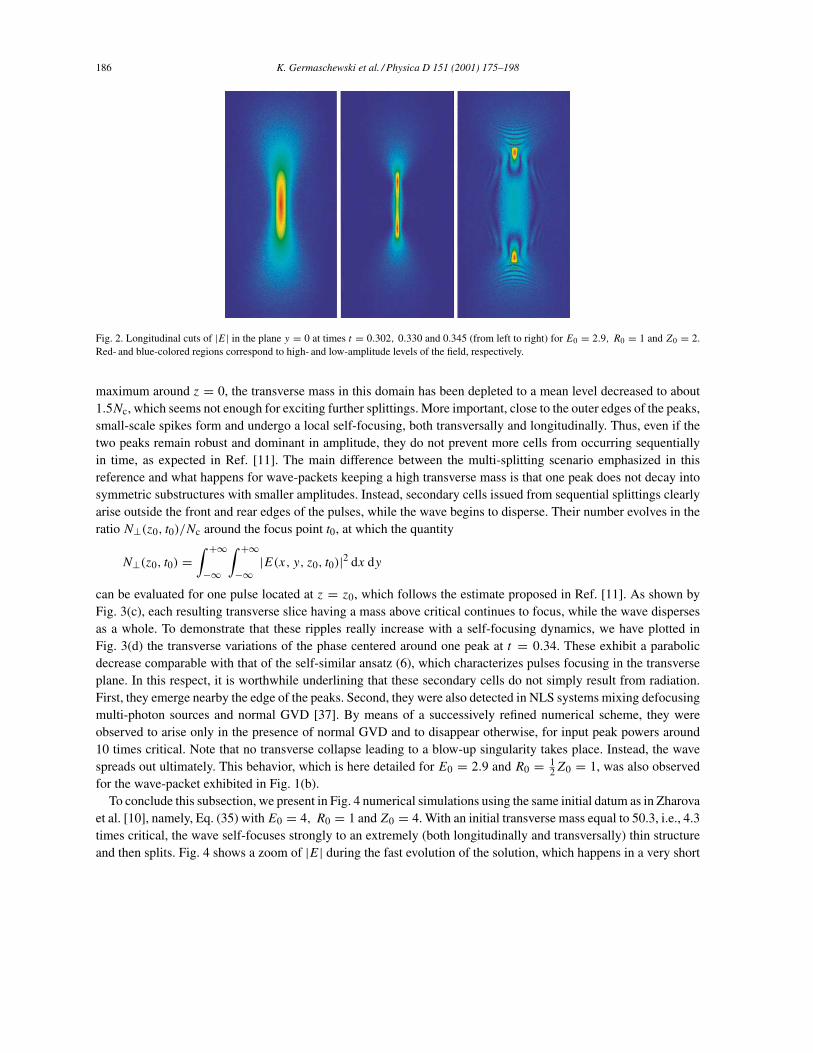
To conclude this subsection, we present in Fig. 4 numerical simulations using the same initial datum as in Zharovaet al. [10], namely, Eq. (35) withE0 = 4, R0 = 1 andZ0 = 4. With an initial transverse mass equal to 50.3, i.e., 4.3times critical, the wave self-focuses strongly to an extremely (both longitudinally and transversally) thin structureand then splits. Fig. 4 shows a zoom of |E| during the fast evolution of the solution, which happens in a very short


Fig. 3. Wave amplitude (top curves), phase (middle) and transverse mass (bottom) versus z for the initial condition E0 = 2.9 used in Fig. 2 andat times (a) t = 0.338, (b) t = 0.34 and (c) t = 0.345. (d) The transverse (horizontal axis) and longitudinal (vertical axis) variations of the phasenear one peak at the instant t = 0.34. Colors from blue to red correspond to a phase from 0 to 2π .

time window. The cut of |E| is zoomed by a factor 64 in each spatial direction, as compared with the initial condition(analogous cuts in Fig. 3 correspond to a zoom by a factor 8 only). From Fig. 4 and the plots of |E(0, 0, z, t)| shownin Fig. 5, we can observe that the main tendency of the wave is still to self-compress and split. This behavior is thusgeneric.

Note that the wave evolution is characterized by sharp gradients of |E| along z. Although the previous scenarioemphasizes that ultimately a collapse will not take place, Fig. 5 indicates, in contrast, that it cannot be definitivelyexcluded that the wavefield may become singular. The singular dynamics could here proceed more from a steep


Fig. 4. Longitudinal cuts of |E| in the plane y = 0 for E0 = 4, R0 = 1 and Z0 = 4, illustrating the wave dynamics at times t = 0.150234,0.150343 and 0.150355 (from left to right).

shock-like effect induced by the violent growth in the longitudinal gradients of the peaks, rather than from thedivergence of their amplitude. However, the numerics strongly saturates and a lack of resolution is encountered attimes t ≥ 0.150355, so that we cannot conclude about the final fate of the wave when E0 is as high as 4. Clearingthis point remains an open issue. Nevertheless, we suspect that the numerical simulations presented in Ref. [10]were under-resolved.

4.2. Thresholds for splitting versus s < 0

A question often addressed in such investigations is to determine how the threshold power, at which the splittingprocess becomes efficient, varies with the dispersion coefficient s [7,8,38]. In [7,8], it was expected that a minimalbound for |s| was necessary to arrest the collapse. For a given power ratio p ≡ N⊥(0)/Nc, this bound was estimatedby ignoring the radial confinement of the wave. It was, in particular, argued that for waves with p � 1, |s| shouldbe larger than a bound of order 0.1p3/2. Unfortunately, transverse powers higher than 1.6Nc remained numericallyunreachable in this reference. On the other hand, by means of a multi-scaled variational approach whose resultswere directly compared with the data of [8], Cerullo et al. [38] recently observed that the “collapse threshold” variedalmost linearly with |s| in a short interval of |s|-values. Here, collapse followed from the fact that for Gaussian

Fig. 5. Amplitude |E| evaluated on the z-axis at the same instants as in Fig. 4.


beams the variational approach is not able to restore the splitting along z, as the test function used in this procedureremains frozen on the initial singly humped Gaussian. In spite of this discrepancy, the procedure used in [38] makesthe variations of the collapse threshold quite predictive for anticipating the variations in the power threshold forthe first splitting event, since the wave must first self-focus before splitting. To examine the incidence of s on thissplitting threshold, we briefly employ the ansatz (25) of Section 2.2, in which we assume that φ is exactly self-similarwith ∂τ φ = 0. This function can be modeled by φ(ξ, ζ ) = φ⊥(ξ) exp(− 1

2ζ2), where φ⊥ is chosen as the ground

state φ0. It is then easy to plug Eq. (25) into the virial expressions (22) and (23) and to obtain a dynamical systemgoverning the scales R(t) and Z(t):

1

4d2t R(t) = α

R3(t)

[1 − pZ(0)√

2Z(t)

], (36)

1

4d2t Z(t) = s2

Z3(t)− spZ(0)√

2R2(t)Z2(t), (37)

where α ≡ ∫ |φ0|2 d�ξ/ ∫ ξ2|φ0|2 d�ξ � 0.845 and where the power ratio p appears from N⊥(0) ≡ [A/Z(0)]∫ |φ0|2 d�ξ . In terms of the initial data, Eq. (36) shows that at t = 0, an unchirped wave can self-focus whenever itsinitial transverse mass exceeds

√2Nc. Assuming that splitting develops once the wave self-focuses, this bound is in

rather good agreement with the values (1.3–1.5)Nc, numerically revealed for some ball-shaped waves [7,8] (R0 =Z0) and elongated-shaped waves as well [19] (Z0 > R0). However, as the splitting is a dynamical process resultingfrom the competition between collapse and spreading along z, Eq. (36) shows that a self-focusing preceding thesplitting requires in factN⊥(0) >

√2NcZ(t)/Z(0). Since from (37) Z(t) increases with a negative s, the threshold

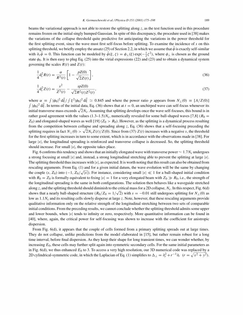
for the first splitting increases in turn to some extent, which is in accordance with the observations made in [38]. Forlarge |s|, the longitudinal spreading is reinforced and transverse collapse is decreased. So, the splitting thresholdshould increase. For small |s|, the opposite takes place.

Fig. 6 confirms this tendency and shows that an initially elongated wave with transverse power ∼ 1.7Nc undergoesa strong focusing at small |s| and, instead, a strong longitudinal stretching able to prevent the splitting at large |s|.The splitting threshold thus increases with |s|, as expected. It is worth noting that this result can also be obtained fromrescaling arguments. From Eq. (1) and for a given initial datum, the wave evolution will be the same by changingthe couple (s, Z0) into (−1, Z0/

√|s|). For instance, considering small |s| � 1 for a ball-shaped initial conditionwith R0 = Z0 is formally equivalent to fixing |s| = 1 for a very elongated beam with Z0 � R0, i.e., the strength ofthe longitudinal spreading is the same in both configurations. The solution then behaves like a waveguide stretchedalong z, and the splitting threshold should diminish to the critical mass for a 2D collapse,Nc. In this respect, Fig. 6(d)shows that a nearly ball-shaped structure (R0/Z0 = 1/

√2) with s = −0.01 still undergoes splitting for N⊥(0) as

low as 1.1Nc and its resulting cells slowly disperse at large z. Note, however, that these rescaling arguments providequalitative information only on the relative strength of the longitudinal stretching between two sets of comparableinitial conditions. From the preceding results, we cannot conclude whether the splitting threshold admits some upperand lower bounds, when |s| tends to infinity or zero, respectively. More quantitative information can be found in[40], where, again, the critical power for self-focusing was shown to increase with the coefficient for anistropicdispersion.

From Fig. 6(d), it appears that the couple of cells formed from a primary splitting spreads out at large times.They do not collapse, unlike predictions from the model elaborated in [15], but rather remain robust for a longtime interval, before final dispersion. As they keep their shape for long transient times, we can wonder whether, byincreasing E0, these cells may further split again into symmetric secondary cells. For the same initial parameters asin Fig. 6(d), we thus enhanced E0 to 3. To access a very high resolution, our 3D numerical code was replaced by a2D cylindrical-symmetric code, in which the Laplacian of Eq. (1) simplifies to�⊥ = ∂2

r + r−1∂r (r =√x2 + y2).


Fig. 6. Variations in the splitting dynamics with respect to the coefficient s when E0 = 2.5, R0 = 1 and Z0 = 2 for (a) s = −0.5, (b) s = −1and (c) s = −2, at different times (from top to bottom): t = 0.3 and 0.505 in the first column, t = 0.3 and 0.7 for the second and third columns.The fourth column (d) shows a waveform analogous to that used in Ref. [15] with E0 = 2.86, R0 = 1/

√2, Z0 = 1 and s = −0.01 at times

t = 0.3 and 1.5.


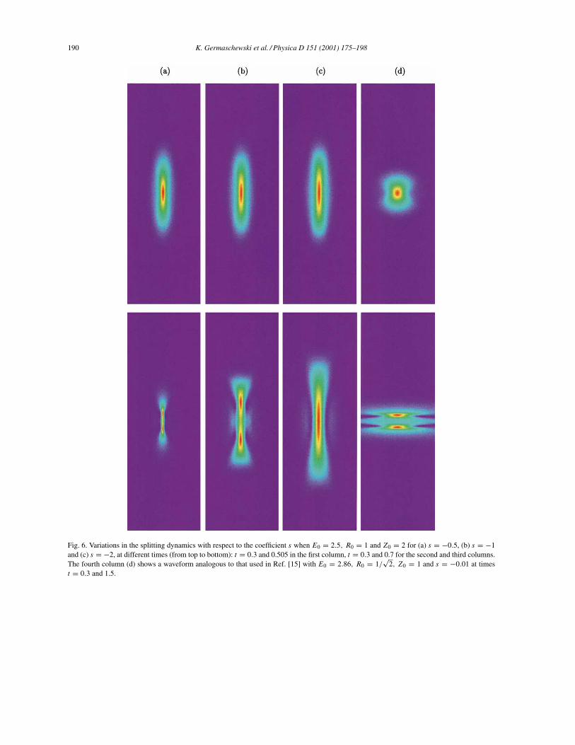
Fig. 7. 3D plots of the amplitude |E| in the (r, z)-plane, obtained from a radially symmetric adaptive mesh refined code, for the initial data usedin Fig. 6(d) with E0 = 3 at times t = 0.4557, 0.4583, 0.4624 and 0.4647 (from left to right). The maximum amplitude attains 27 times E0 atthe instant t � 0.46.

An effective resolution of 245762 could then be reached. The result is shown in Fig. 7, where only the evolutionof one peak is represented. This figure displays evidence of sequentially split structures. The peak first tends to bedivided in its middle (see the first two frames in Fig. 7). However, instead of undergoing a dichotomy yielding asymmetric splitting, it again produces cells recurrently formed near its outer edge only. Even if the peak amplitude isable to reach maxima attaining almost 30 times the initial beam valueE0, the pulse finally spreads out by generatingcells localized nearby its shock front. This property, already revealed in Section 4.1, is here clearly confirmed.

4.3. Monitoring single/multiple splittings

As can be inferred from the above simulations, the sequential division of the wave into equally symmetric splitpulses seems not generic, at least from the initial data considered here. Instead, small-scale cells develop near theouter edge of the pulse, which assures the dispersion of the wave. It is thus worthwhile identifying the mechanismsthat can stop the development of further symmetric splittings, after the primary splitting event. For this purpose,we monitor the splitting by preconditioning the amplitude and phase of the initial solution. First, we employ theGaussian-shaped initial conditionE(x, y, z, 0) = E0 ×(G++G−), whereG± are the two Gaussian input functions

G±(x, y, z) = exp

[−x

2 + y2

2R20

− (z±�z)2

2Z20

]. (38)

From this ansatz, it is possible to determine, for a given initial amplitudeE0, the mutual separation distance δ = 2�zsupporting a critical value δc, above which each of the Gaussian components freely splits up and below which splittingmay be inhibited. Fig. 8 shows the results, starting with E0 = 2.5. For δ larger than 7, it is seen right away that eachGaussian splits individually as the interaction between Gaussian tails is negligible. For δ belonging to the range5 < δ < 7, the two inner pulses created from splitting merge into one self-focusing lobe that ultimately splits inturn. At lower distances δ ≤ δc = 5, the process of individual splitting is aborted, in the sense that the two Gaussiansself-focus and reform a singly split pattern, where each pulse undergoes a focusing dynamics. Below δ = 4, theGaussian components overlap so much, that they cannot be distinguished from one another. Their mutual interactionis so strong that they only form one lobe, which tends to collapse. In that case, the collapse is reinforced by thefact that, initially, the wave amplitude exhibits a flat plateau along z, i.e., the z derivatives for such an elongatedstructure are close to zero.

In order to justify these interaction regimes, we employ qualitative arguments previously used in Ref. [39] forexplaining the fusion of 2D self-focusing filaments. First, by means of expression (38), it is readily found that thetotal mass of the wave, N = ∫ |E|2 d�r dz, is expressed as

N(δ) = 2Z0√πN⊥(0)(1 + e−δ2/4Z2

0 ). (39)


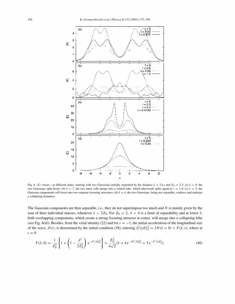
Fig. 8. |E| versus z at different times, starting with two Gaussians initially separated by the distance δ = 2�z and E0 = 2.5. (a) δ = 8, thetwo Gaussians split freely; (b) δ = 7, the two inner cells merge into a central lobe, which afterwards splits again at t = 1.4; (c) δ = 5, theGaussian components self-focus into two separate focusing structures; (d) δ = 4, the two Gaussians, being not separable, coalesce and undergoa collapsing dynamics.

The Gaussian components are then separable, i.e., they do not superimpose too much and N is mainly given by thesum of their individual masses, whenever δ > 2Z0. For Z0 = 2, δ > 4 is a limit of separability and at lower δ,both overlapping components, which create a strong focusing attractor at center, will merge into a collapsing lobe(see Fig. 8(d)). Besides, from the virial identity (22) and for s = −1, the initial acceleration of the longitudinal sizeof the wave, Z(t), is determined by the initial condition (38), entering ∂2

t ‖zE‖22 = 2N(δ = 0)× F(δ, t), where at

t = 0

F(δ, 0) = 1

Z20

{1 +

(1 − δ2

2Z20

)e−δ2/4Z2

0

}+ E2

0

4√

2{1 + 4 e−3δ2/8Z2

0 + 3 e−δ2/2Z20 }. (40)


The initial enhancement of Z(t) varies with the strength of the interaction between the Gaussians. For Z0 =2, E0 = 2.5, F (δ, 0) exponentially decreases for 4 < δ < 7. In this range, the interaction is dominant through theleading-order term (1 − δ2/2Z2

0) e−δ2/4Z20 coming from the longitudinal gradients, which contributes to slow down

the increase ofZ(t) at times t > 0. For δ < 7, the Gaussian components cannot split freely and the total length of thewave-packet is reduced. For 7 ≤ δ ≤ 8, F (δ, 0) attains its minimal value ∼1.35 and the interaction terms becomesmaller. The Gaussians thus split and weakly interact, while the total longitudinal size Z(t) does not significantlychange, at least in the early evolution. From δ > 8, F (δ, 0) forms a plateau around ∼1.37, i.e., slightly above itsformer value, and the interaction terms rapidly decrease to zero. The longitudinal scale of the whole wave-packetmay thus increase to a little extent, while each Gaussian splits freely. These qualitative behaviors agree with thenumerical results displayed in Fig. 8. From a quantitative viewpoint, they, however, do not provide the exact criticalvalues of δ separating the different interaction regimes.

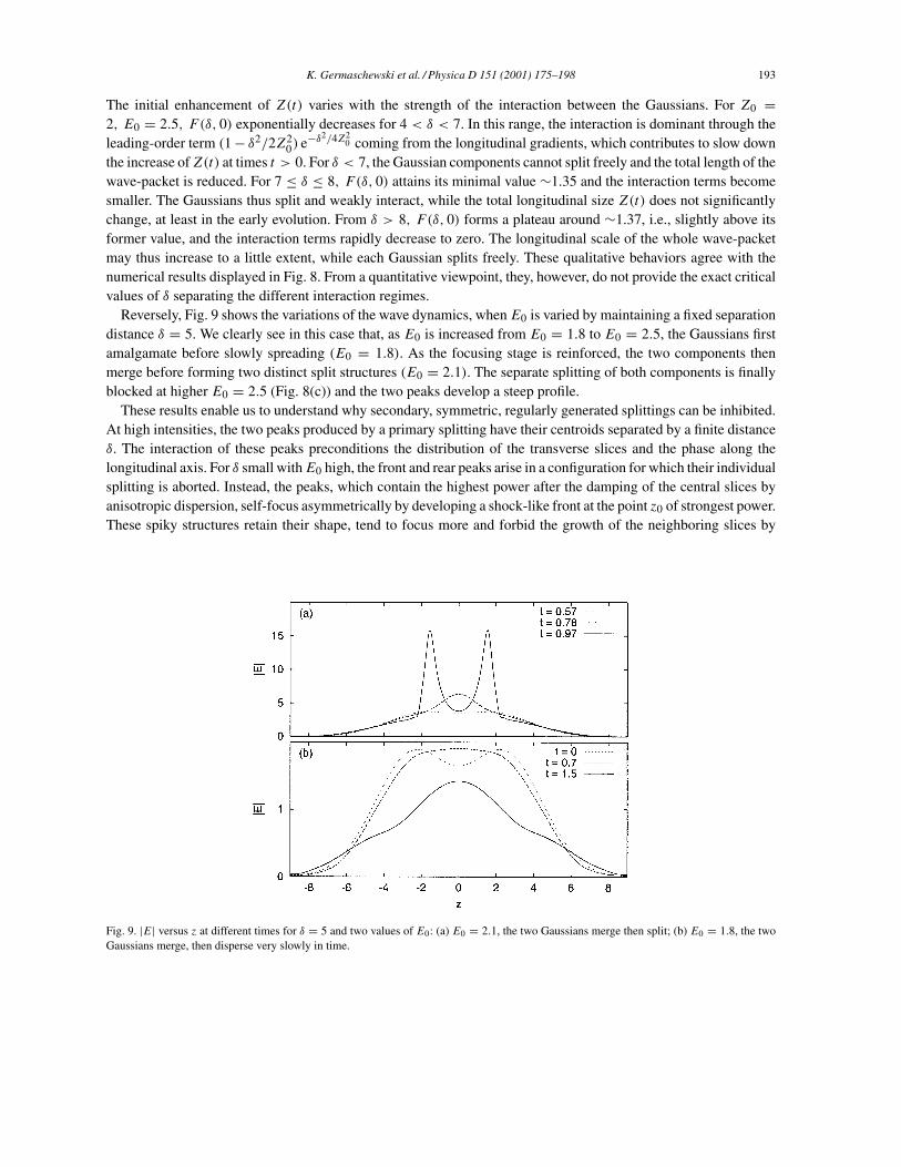
Reversely, Fig. 9 shows the variations of the wave dynamics, whenE0 is varied by maintaining a fixed separationdistance δ = 5. We clearly see in this case that, as E0 is increased from E0 = 1.8 to E0 = 2.5, the Gaussians firstamalgamate before slowly spreading (E0 = 1.8). As the focusing stage is reinforced, the two components thenmerge before forming two distinct split structures (E0 = 2.1). The separate splitting of both components is finallyblocked at higher E0 = 2.5 (Fig. 8(c)) and the two peaks develop a steep profile.

These results enable us to understand why secondary, symmetric, regularly generated splittings can be inhibited.At high intensities, the two peaks produced by a primary splitting have their centroids separated by a finite distanceδ. The interaction of these peaks preconditions the distribution of the transverse slices and the phase along thelongitudinal axis. For δ small withE0 high, the front and rear peaks arise in a configuration for which their individualsplitting is aborted. Instead, the peaks, which contain the highest power after the damping of the central slices byanisotropic dispersion, self-focus asymmetrically by developing a shock-like front at the point z0 of strongest power.These spiky structures retain their shape, tend to focus more and forbid the growth of the neighboring slices by

Fig. 9. |E| versus z at different times for δ = 5 and two values of E0: (a) E0 = 2.1, the two Gaussians merge then split; (b) E0 = 1.8, the twoGaussians merge, then disperse very slowly in time.


mutual attraction. Reversely, when they disperse (Figs. 3 and 7), this attraction is relaxed and the neighboring sliceswith mass above critical are then able to focus.

Besides, it is possible to modify artificially the phase of one peak formed through the splitting process and observethe fate of the resulting solution. For this purpose, we have deleted the sharp variations in the phase of E aroundone of the peaks originating from the splitting of a beam with E0 = 2.9, R0 = 1, Z0 = 2, and let the solutionevolve again. After doing so, we observed that the solution reorganized itself. It systematically reproduced the shapecommented in Fig. 3 and again formed small-scale ripples. Formation of such spiky structures is thus a genericproperty of high-power beams governed by Eq. (1). On the other hand, it is now well known that the introductionof a phase chirp in the form e−iCz2

with C < 0 can prefocus the wave and strongly influence its compression stagealong z [19]. Connecting this property with the expression (25), this amounts to introducing Zt(0) < 0 for favoringa longitudinal compression. To control the separation of the pulses and favor the formation of split structures, welooked at the effects of such a longitudinal chirp. In Fig. 10, we have introduced a shrinking chirp with differentvalues Zt(0) < 0 into an initial wave that does not naturally split when it is unchirped (E0 = 2.3, Fig. 10(a)).The longitudinal compression induced by the chirp clearly results in triggering the splitting for E0 = 2.3, R0 =1, Z0 = 2 (Figs. 10(b) and (c)). Fig. 10(d) shows the chirp influence on higher amplitude waves (E0 = 2.9), thatalready split without chirp. The induced variations in the phase make the wave more confined towards the centerz = 0, which results in a nearly collapsing structure that eventually splits up. The chirp-induced shrinking effectarises before the first two peaks form and it accelerates their formation. From the initial data investigated, it seemsnot to produce more than two symmetric peaks, but can still generate secondary ripples.

Fig. 10. Longitudinal cuts of an initially chirped wave with R0 = 1, Z0 = 2 favoring the development of splitting events in different situations,for which each couple of figures refers to two instants increasing from top to bottom: (a) C = 0, E0 = 2.3 for t = 0.3 and 0.7; (b)C = −0.2, E0 = 2.3 for t = 0.3 and 0.7; (c) C = −1, E0 = 2.3 for t = 0.2 and 0.251; (d) C = −0.2, E0 = 2.9 for t = 0.27 and 0.283. Thelast pictures at final times in (c) and (d) have been magnified by a factor 5.


5. Modulational instability of 2D waveguides: interplay of bunches and snakes

Eq. (1) promotes modulational instabilities giving rise to two kinds of patterns, namely (i) “bunches”, resultingfrom the periodic break-up of a soliton waveguide φ0 by even perturbations and (ii) “snakes”, resulting from thebending distortions of the same waveguide by odd modes. Following the summary in Section 2.3, φ0 is even in thetransverse variable and (�r/r)∂rφ0 is odd, so that the family of perturbations that is expected to efficiently destabilizethe soliton φ0 can be chosen as entering the following initial condition:

E(x, y, z, t = 0) = {1 + ε cos(kz)(i + ∂x)}φ0(x, y), ε � 1. (41)

For numerical convenience and since bound states φ0 are rather close to Gaussians, we decided to investigate thetemporal evolution of bunch/snake modes by means of perturbed Gaussian waveguides. Instead of Eq. (41), we thusperturb a Gaussian solution with small-scale modulations entering

E(x, y, z, t = 0) = {1 + cos(kz)(iεb + εs∂x)}Ein(x, y), (42)

Ein(x, y) ≡ E0 exp

[−x

2 + y2

2R20

]. (43)

Here, εb � 1 and εs � 1 are the small parameters that separately fix the amplitudes of bunch-type and snake-typeperturbations. In Eq. (42), k is the instability wavenumber, which, in connection with standard results [29–31], ischosen of order unity (k = 1–5) to emphasize the number of bunch/snake structures and their mutual competitioninside our numerical box.

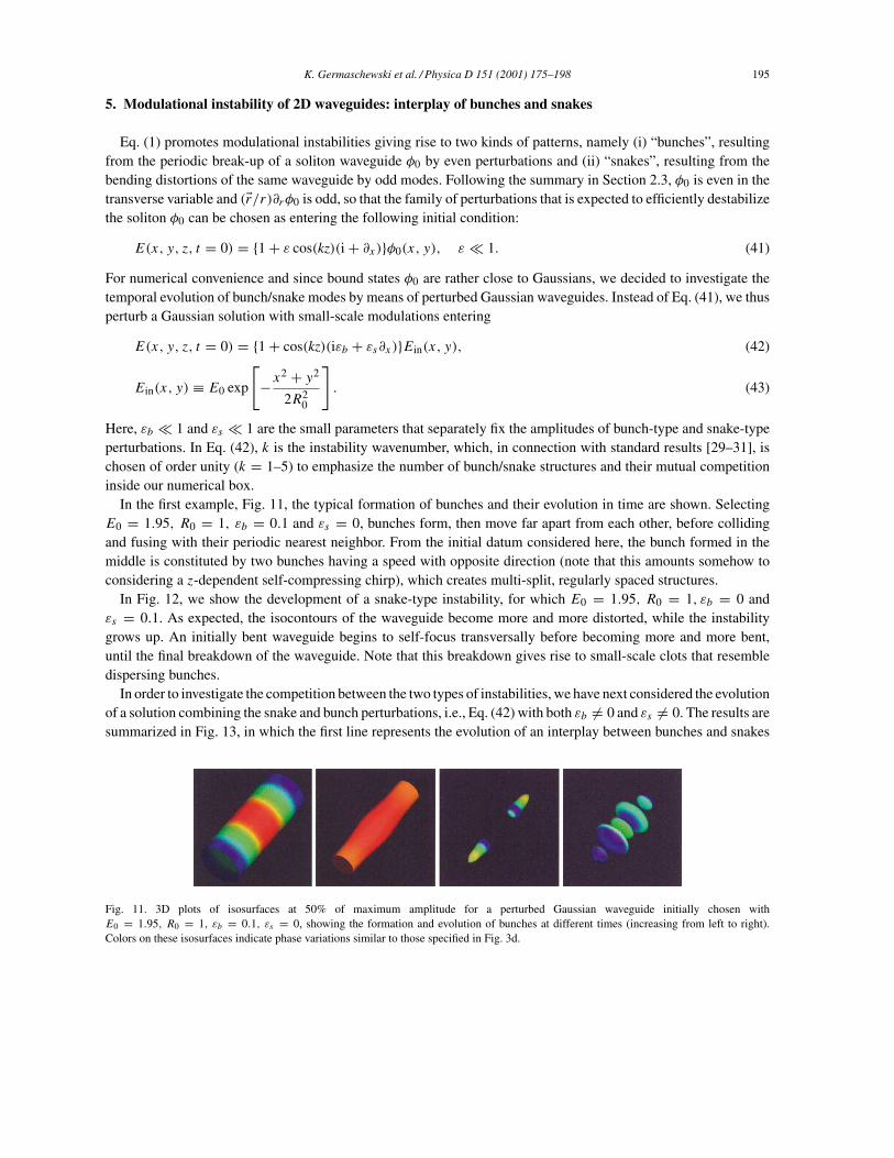
In the first example, Fig. 11, the typical formation of bunches and their evolution in time are shown. SelectingE0 = 1.95, R0 = 1, εb = 0.1 and εs = 0, bunches form, then move far apart from each other, before collidingand fusing with their periodic nearest neighbor. From the initial datum considered here, the bunch formed in themiddle is constituted by two bunches having a speed with opposite direction (note that this amounts somehow toconsidering a z-dependent self-compressing chirp), which creates multi-split, regularly spaced structures.

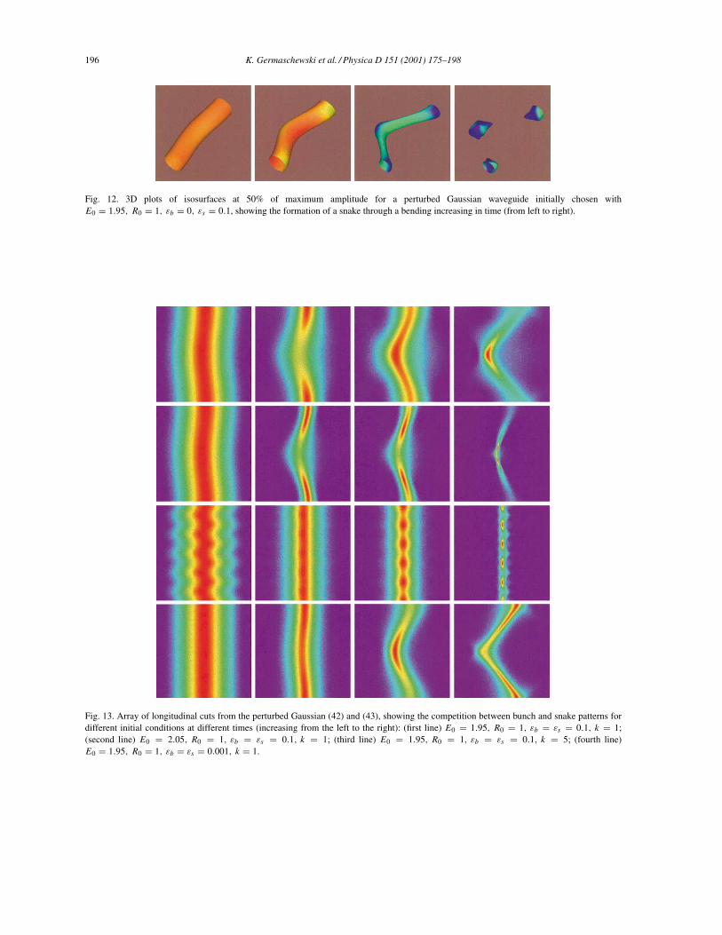
In Fig. 12, we show the development of a snake-type instability, for which E0 = 1.95, R0 = 1, εb = 0 andεs = 0.1. As expected, the isocontours of the waveguide become more and more distorted, while the instabilitygrows up. An initially bent waveguide begins to self-focus transversally before becoming more and more bent,until the final breakdown of the waveguide. Note that this breakdown gives rise to small-scale clots that resembledispersing bunches.

In order to investigate the competition between the two types of instabilities, we have next considered the evolutionof a solution combining the snake and bunch perturbations, i.e., Eq. (42) with both εb �= 0 and εs �= 0. The results aresummarized in Fig. 13, in which the first line represents the evolution of an interplay between bunches and snakes

Fig. 11. 3D plots of isosurfaces at 50% of maximum amplitude for a perturbed Gaussian waveguide initially chosen withE0 = 1.95, R0 = 1, εb = 0.1, εs = 0, showing the formation and evolution of bunches at different times (increasing from left to right).Colors on these isosurfaces indicate phase variations similar to those specified in Fig. 3d.


Fig. 12. 3D plots of isosurfaces at 50% of maximum amplitude for a perturbed Gaussian waveguide initially chosen withE0 = 1.95, R0 = 1, εb = 0, εs = 0.1, showing the formation of a snake through a bending increasing in time (from left to right).

Fig. 13. Array of longitudinal cuts from the perturbed Gaussian (42) and (43), showing the competition between bunch and snake patterns fordifferent initial conditions at different times (increasing from the left to the right): (first line) E0 = 1.95, R0 = 1, εb = εs = 0.1, k = 1;(second line) E0 = 2.05, R0 = 1, εb = εs = 0.1, k = 1; (third line) E0 = 1.95, R0 = 1, εb = εs = 0.1, k = 5; (fourth line)E0 = 1.95, R0 = 1, εb = εs = 0.001, k = 1.


forE0 = 1.95, εb = εs = 0.1 and k = 1. The second line of pictures shows the same mixing of bunches and snakesat higher initial amplitude E0 = 2.05. Third line displays formation of multiple bunches and snakes originatingfrom Eqs. (42) and (43), when a larger wavenumber k = 5 is selected forE0 = 1.95. Finally, for k = 1, E0 = 1.95,bunches and snakes interplay in the fourth line from a low-valued perturbation amplitude εb = εs = 0.001. Fromthese pictures, it appears that in most of cases the bunch-like instability wins: although the waveguide first undergoesa bending, small-scale bunches form in the bent structure and the end dynamics looks like that shown in Fig. 11.Bunches either survive or fuse into one central lobe after the initial bending (see, e.g., first and second rows inFig. 13). The centroid of the resulting structure is then more or less displaced by the snake instability. At high initialamplitude, the formation of small-scale bunches may be enhanced by the splitting dynamics. At lower powers orweaker ε, the development of “snakes” is, however, more pronounced in the early dynamics of the modulationalinstability. We attribute this property to the fact that in the low-perturbative limit (ε = 0.001), the growth rate ofsnakes, γ 2

snake ∼ k2, can exceed that of bunches, γ 2bunch ∼ k, for k close to unity.

As a result, only perturbing slightly an initial Gaussian can give rise to complicated patterns which depart fromthe standard primary splitting addressed in, e.g. [14], where, in this regard, perturbed Gaussians were employed forexplaining the occurrence of one splitting event. Definitively, our numerical simulations show that Eq. (1) containsa much richer dynamics than a single splitting: Even for very slightly perturbed initial data, it can describe waveevolutions involving multi-split structures, spatio-temporal distortions and coalescence of wave-packets, comparablewith those emphasized in, e.g. Ref. [16], where focusing optical beams were modeled by means of extended NLSsystems that included, moreover, nonlinear asymmetric effects.

6. Conclusion

We have investigated the dynamics of perturbed and unperturbed Gaussian solutions to the 3D NLS equation(1) with anisotropic dispersion. After recalling the main theoretical expectations in the field, it has been shownby means of a numerical code elaborated on an adaptive mesh refinement solver that in media with anisotropicdispersion self-focusing wave-packets created from a primary splitting can generate smaller-amplitude ripple-likecells focused with a transverse mass above critical. These cells emerge while the wave disperses as a whole. Formoderate initial intensities, this scenario departs from the “symmetric” picture of multiple splitting given in Refs.[11,19], since secondary spikes only develop in the far edge of the wave, as the two main peaks keep a steepshock-like profile while they interact. In spite of this limitation, Eq. (1) does promote the formation of secondarysplit structures, sequentially excited after the first splitting event. We believe that this decay into multiple structuresasymmetrically emitted from the edge of the pulses provides a generic way for saturating the collapse and dissipatingthe wave energy. This scenario was observed as a dynamics always regularizing the collapse for several values of thedispersion coefficient (−2 ≤ s ≤ −0.01), various anisotropy ratios R0/Z0, and initial amplitudes (2 < E0 < 4).It does not exclude, a priori, other sets of initial conditions to produce symmetric multiple splittings.

Another generic feature is that collapse promoting a blow-up singularity was never observed in high-powersolutions of Eq. (1). In particular, no transverse blow-up was detected. Also, even though the solution undergoes sharpgradient growths along the z-axis, these ultimately lead to a longitudinal stretching of the waveform, which avoidsforming a local singularity. This property seems generic for high-amplitude solutions to Eq. (1) withN⊥(0) < 6Nc,but it would need to be confirmed for higher amplitudes by using a better resolution in future works. For instance,Fig. 5 points out that very intense waves may yield a singularity that should differ from a critical collapse, becauseof the peculiar growth in the longitudinal gradients. In the present state, our numerics cannot identify the final fateof such wave-packets.

Finally, we have investigated the two different patterns developed through the modulation instability of Gaussian-type waveguide solutions, localized in the transverse plane and perturbed along the z-axis. After identifying bunches


and bending-type (snake) instabilities, it has been shown that, at least for wave-packets with high enough mass,bunch dynamics mainly drives the instability of waveguides after a first focusing stage. Although the waveguideundergoes a clear bending in the early quasi-linear evolution, small-scale bunches generally seem to be producedat later stages, to the detriment of snaked distortions.

Acknowledgements

This work was supported by INTAS Grant 96-0413 and by SFB 191. It was initiated at the First Nonlinear ScienceFestival organized by the Graduate School in Nonlinear Science and CATS at the Niels Bohr Institute, Universityof Copenhagen, December 1998.

References

[1] J.R. Myra, C.S. Liu, Phys. Fluids 23 (1980) 2258.[2] A.G. Litvak, T.A. Petrova, A.M. Sergeev, A.D. Yunakovskii, Fiz. Plazmy 9 (1983) 495 [Sov. J. Plasma Phys. 9 (1983) 287].[3] A.C. Newell, J.V. Moloney, Nonlinear Optics, Addison-Wesley, Redwood City, CA, 1991.[4] J. Juul Rasmussen, K. Rypdal, Phys. Scripta 33 (1986) 481.[5] L. Bergé, Phys. Rep. 303 (1998) 259.[6] J.E. Rothenberg, Opt. Lett. 17 (1992) 583.[7] P. Chernev, V. Petrov, Opt. Commun. 87 (1992) 28.[8] P. Chernev, V. Petrov, Opt. Lett. 17 (1992) 172.[9] G.G. Luther, A.C. Newell, J.V. Moloney, Physica D 74 (1994) 59.

[10] N.A. Zharova, A.G. Litvak, T.A. Petrova, A.M. Sergeev, A.D. Yunakovskii, Pis’ma Zh. Eksp. Teor. Fiz. 44 (1986) 12 [JETP Lett. 44 (1986)13].

[11] L. Bergé, J. Juul Rasmussen, Phys. Plasmas 3 (1996) 824.[12] J.K. Ranka, R.W. Schirmer, A.L. Gaeta, Phys. Rev. Lett. 77 (1996) 3783.[13] S.A. Diddams, H.K. Eaton, A.A. Zozulya, T.S. Clement, Opt. Lett. 23 (1998) 379.[14] G. Fibich, G.C. Papanicolaou, Phys. Rev. A 52 (1995) 4218.[15] G. Fibich, G.C. Papanicolaou, SIAM J. Appl. Math. 60 (1999) 183.[16] A.A. Zozulya, S.A. Diddams, A.G. Van Engen, T.S. Clement, Phys. Rev. Lett. 82 (1999) 1430.[17] L. Bergé, J. Juul Rasmussen, M.R. Schmidt, Phys. Scripta T75 (1998) 18.[18] M.R. Schmidt, Ph.D. Thesis, Risø Report R-1076, 1999.[19] L. Bergé, J. Juul Rasmussen, E.A. Kuznetsov, E.G. Shapiro, S.K. Turitsyn, J. Opt. Soc. Am. B 13 (1996) 1879.[20] C. Sulem, P.L. Sulem, The Nonlinear Schrödinger Equation: Self-focusing and Wave Collapse, Applied Mathematical Sciences, Vol. 139,

Springer, Berlin, 1999 (Chapter 9).[21] R.T. Glassey, J. Math. Phys. 18 (1977) 1794.[22] S.N. Vlasov, V.A. Petrishchev, V.I. Talanov, Izv. Vuz. Radiofiz. 14 (1971) 1353 [Radiophys. Quant. Electron. 14 (1974) 1062].[23] M.I. Weinstein, Commun. Math. Phys. 87 (1983) 567.[24] G.M. Fraiman, Zh. Eksp. Teor. Fiz. 88 (1985) 390 [Sov. Phys. JETP 61 (1985) 228].[25] V.M. Malkin, Phys. Lett. A 151 (1990) 285.[26] M. Landman, G.C. Papanicolaou, C. Sulem, P.L. Sulem, Phys. Rev. A 38 (1988) 3837.[27] B. LeMesurier, G.C. Papanicolaou, C. Sulem, P.L. Sulem, Physica D 32 (1988) 210.[28] L. Bergé, E.A. Kuznetsov, J. Juul Rasmussen, Phys. Rev. E 53 (1996) R1340.[29] V.E. Zakharov, A.M. Rubenchik, Zh. Eksp. Teor. Fiz. 65 (1973) 997 [Sov. Phys. JETP 38 (1974) 494].[30] E.A. Kuznetsov, A.M. Rubenchik, V.E. Zakharov, Phys. Rep. 142 (1986) 103.[31] K. Rypdal, J. Juul Rasmussen, Phys. Scripta 40 (1989) 192.[32] M.J. Berger, P. Colella, Comput. Phys. 82 (1989) 64.[33] H. Friedel, R. Grauer, C. Marliani, J. Comput. Phys. 134 (1997) 190.[34] H. Pietsch, E.W. Laedke, K.H. Spatschek, Phys. Rev. E 47 (1993) 1977.[35] W. Hackbusch, Iterative Solution of Large Sparse Systems of Equations, Springer, New York, 1994.[36] R. Grauer, C. Marliani, K. Germaschewski, Phys. Rev. Lett. 80 (1998) 4177.[37] L. Bergé, A. Couairon, Phys. Plasmas 7 (2000) 210.[38] G. Cerullo, A. Dienes, V. Magni, Opt. Lett. 21 (1996) 65.[39] L. Bergé, M.R. Schmidt, J. Juul Rasmussen, P.L. Christiansen, K.∅. Rasmussen, J. Opt. Soc. Am. B 14 (1997) 2550.[40] G.G. Luther, A.C. Newell, J.V. Moloney, E.M. Wright, Opt. Lett. 19 (1994) 862.

Documents

Splittings, coalescence, bunch and snake patterns in the 3D …mezentsv/papers/PD-v151-p175.pdf · Splittings, coalescence, bunch and snake patterns in the 3D nonlinear Schrödinger