Embed Size (px)
Citation preview

Spill Over Covid-19 and Indices around the Globe
Dwi Pramaya Bhakti and Hidajat Sofyan Widjadja
Both are lecturer of Perbanas ABFI Jakarta
Abstract
The impact of Covid-19 has had implications for all aspects of life, especially in the economic
sector. Measurement of the impact of the pandemic has been carried out by all countries in the
world without exception. The different patterns of the impact of Covid-19 on the economic cycle
in each country are different depending on the initial impact until it reaches its peak. For example,
China has experienced the peak of Covid-19 in early 2020. Italy and several European countries
in April and May 2020. The United States including Indonesia in November and December 2020.
Finally, India has only experienced the peak of Covid-19 in May 2021. This is also what has caused
economic policy makers in various countries to apply different patterns. Indonesia as a country
with a very open economy has implemented major social restrictions in various cities throughout
Indonesia, especially those related to other countries. This research will use a combination of
cross-section and time series data which will then be processed by panel data. The data used is
the number of confirmed Covid-19 countries between March 2020 and May 2021. This timing is
based on the pattern of Covid-19 influence that has spread throughout the world An important
finding from this study is that the covid-19 variable greatly influences the stock price index in the
USA, INDONESIA and KSA during the study period. But for the long term, the variables Gold and
Crude oil will again be the main determinants of the global index.
Keywords: COVID-19, Vector Autoregressive (VAR), Indonesian Stock Market and World
Indices
JEL Classification: C22, G11, G15, C32
Introduction
The impact of Covid-19 has had implications for all aspects of life, especially in the
economic sector. Measurement of the impact of the pandemic has been carried out by all countries
in the world without exception. The impact of COVID-19 on all countries has caused a slowdown
in economic growth in almost all of the world. The different patterns of the pandemic from one
country to another cause the handling to be different. if China has been free from the covid-19
pandemic, it is precisely when almost all countries in the world are struggling to fight the pandemic
in early March 2020. Europe, in this case Italy, followed by France, Germany and the UK, have
fought against the pandemic in April to July of the same year. followed by the United States, which
struggled against the pandemic in November and December 2020. Indonesia was among the worst
hit in mid-March 2020, but the peak of the pandemic was only seen in November and December
in 2020.
Research on the impact of Covid-19 on economic performance is very massive in the
scientific world, both the branch of economics itself and its derivatives as well as a wider
dimension. During 2020 and currently entering the second half of 2021, research on the impact of
covid-19 is still being carried out considering the impact and spectrum of this pandemic is very
broad in the dimensions of human life in the modern era. This pandemic has a greater impact on

the economy and other dimensions than previous pandemics such as the Spanish Flu in the early
20th century and the pandemic in the late 20th and early 21st centuries.
This study will reveal in detail the types and impacts of research from several researchers
which will be explained in the next section, namely the study of literature. Furthermore, the author
will try to do a hypothesis on this research. The next section is a brief discussion of the research
methodology. Next is to discuss the regression results and analyze them. The final part is
conclusion and discussion.
Literature Study
The COVID-19 pandemic proved to be a true black swan (Thaleb, NN, 2007); completely
unexpected, it may be remembered as one of the most significant, widespread events affecting the
global financial markets, economies, and all of humanity. Its rapid spread has also demonstrated
the dark side of globalisation and how intense may be a global spillover effect between
countries.(Zeremba, and all 2020). The outbreak itself, as well as the ensuing spiral of containment
and closure policies, led to an unprecedented economic and financial downturn not witnessed for
decades since the Great Depression, which is believed to be very different from any previous
downswings (Bernanke, 2020; Reinhart, 2020), and far worse than the Global Financial Crisis
(Fund, 2020).
Wang and Enilov (2020) use panel Granger non-causality tests to investigate the impact of
COVID-19 cases on stock market returns in the G7 countries. For Canada, France, Germany, Italy,
and the US, the causality runs from COVID-19 cases to stock market returns, while mixed results
obtain for the UK, and no relationship is documented for Japan.
Nader Alber (2020) attempts to investigate the effects of Coronavirus spread on stock
markets using panel data analysis, on daily basis over the period from March 1, 2020 until
September 30, 2020. Coronavirus spread has been measured by daily cases and daily deaths per
million of population, while stock return is measured by Δ in sectoral indices. This has been
conducted after dividing the research period into 6 months from March to September and has been
applied on 17 sectors in the Egyptian Exchange.
Beirne, Renzhi, Sugandi, and Volz (2020) empirically examines the reaction of global
financial markets across 38 economies to the COVID-19 outbreak, with a special focus on the
dynamics of capital flow across 14 emerging market economies. Using daily data over the period
4 January 2010 to 30 April 2020 and controlling for a host of domestic and global macroeconomic
and financial factors, we use a fixed effects panel approach and a structural VAR framework to
show that emerging markets have been more heavily affected than advanced economies.
What determines a country’s financial immunity to a global pandemic? To answer this
question, Zeremba and All (2020) investigated the behavior of 67 equity markets around the world
during the COVID-19 outbreak in 2020. They consider a multidimensional data set that includes
factors from finance, economic, demographics, technological development, healthcare,
governance, culture and law.
Ramelli and Wagner (2020) discuss the impact of US firms’ trade and financial policies on
US stock prices during the COVID-19 pandemic. They make the point that investors retreated
from the stocks of US firms that were highly exposed to the People’s Republic of China (PRC), in
line with the traditional response of markets to increase in times of uncertainty. As the virus spread
to Europe and the US, investors became more concerned about the financial conditions of firms
located in these areas, particularly those with high debt and/or low liquidity, with negative
repercussion for stock prices/

Baker et al. (2020) find that the impact of COVID-19 on US stock market volatility is much
greater than that of previous pandemics that occurred since the year 1900, in particular due to the
economic ramifications of containment policies.
Maroua & Slim (2020) aim to examine the effect of COVID-19 pandemic on stock market
in KSA applying an Autoregressive Distributed Lag (ARDL) cointegration approach. More
especially, it analyzes the relationship between the natural logarithm of trading volume of Tadawul
All shares index (TASI) and the natural logarithm of daily COVID-19 confirmed cases in both the
short-run and the long-run. The bounds test for cointegration is carried out for daily series over the
period from March 02, 2020 until May 20, 2020.Toda-Yamamoto causality test is implemented
between variables. The results indicate that there is a negative impact of COVID-19 on stock
market only in the long-run. Causality test reveals a unidirectional causality from COVID-19
prevalence’s measure to stock market. Robustness check seems to be conclusive.
Thakur (2020) attempts to investigate the movement of US stock market during the COVID
19 pandemic. The paper has used time series analysis using Vector Autoregression (VAR) model
using data from Jan 23, 2020 to June 19, 2020. The finding suggests that Standard and Poor Index
which has been used as reference for capital market has shown negative causality with increase in
number of new cases at global level.
Alber & Saleh (2020) attempts to investigate the effects of 2020 Covid-19 world-wide
spread on stock markets of GCC countries. Findings show that there are significant differences
among stock market indices during the research period. Besides, stock market returns seem to be
sensitive to Coronavirus new deaths. Moreover, this has been confirmed for March without any
evidence about these effects during April and May 2020. Moreover, Smales (2020) addresses the
investor attention and the response of US Stock sectors to the COVID-19 crisis from Dec., 31,
2019 to May, 31, 2020. This has been conducted using the S&P500 Composite Index and
considering returns on the 11 sectors within the Global Industry Classification Standard (GICS).
Gormsen and Koijen (2020) use data from the aggregate stock market and dividend futures
to quantify how investors’ expectations about economic growth evolve across horizons in response
to the coronavirus outbreak and subsequent policy responses in both US and EU until June 2020.
Dividend futures, which are claims to dividends on the aggregate stock market in a particular year,
can be used to directly compute a lower bound on growth expectations across maturities or to
estimate expected growth using a forecasting model.
Methodology
Methodology of VAR in Matrix
Furthermore, Granger causality test between the variables studied in the vector error
correction framework (VECM). Before carrying out this stage, the stages in the Granger causality

test are to perform a stationary test and co-integration between the observed variables. The ADF
test (The Augmented Dickey-Fuller) has been used to study stationary variables in time-series data
from studies to find the order of integration between variables. The ADF test has been carried out
by estimating the regression as follows. (Bhakti, D.P, 2018)
ΔYt= α0 + α1 Yt-1 + Σ γj ΔYt-j + εt
The ADF test is based on the Zero Hypothesis, where H0: Yt is not 1 (0). If the ASF statistic
is less than the critical value, then the null hypothesis is rejected, otherwise if the ADF value
exceeds the critical value, then H0 is accepted. If the variable to be tested is stationary at that level,
the variable is said to be integrated with zero order. I(0). If the variable is at a non-stationary level,
then an ADF test is performed and a first difference test is performed on the variables used for the
unit root test. The variable is said to be co-integrated in the 1st Order, I (1), that is, if it has a
stationary variable completeness.
The next stage is to test Johansen's co-integration test which has been applied to examine
whether long-term equilibrium occurs between variables. Johansen's approach to the co-
integration test is based on 2 statistical tests. First, looking for statistical tests, second looking for
the maximum Eigen value in statistical tests. The search for statistical tests can be specified as
follows:
τ trace = -T Σ log (1-λi),
Where λ is the largest Eigen value in the matrix Π, and T is the number of observations.
In the search test, Hypothesis Zero is the number of different co-integrating vectors (s) less than
or equal to the number of co-integrating relationships (r). The maximum Eigen value test studies
the null hypothesis whose value is equal to r or the integration relationship to the alternative
relationship r+1 with statistical tests.
λ max = -T log (1- λ r+1 ). Where λ r+1 is (r+1) of the largest root Eigen value. In the
search test, the null hypothesis, r = 0 is tested against the alternative r+1 of the co-integrating
vector. At the end, Granger Causality Test has been used to determine whether a time series is
useful in predicting other variables, so as to find directions and relationships between variables in
the study. Co-integration between two stationary variables has been tested by Johansen Trace and
maximum Eigen value test.
In the Granger causality test, the vector in the endogenous variable is divided into 2 sub-
vectors, Y1t and Y2t with dimensions K1 and K2 separately, so, K = K1 + K2. The sub vector Y1t
is said to be Granger-causal to Y2t if it contains important information to predict the next set of
variables. To test this property, the VAR ratings that follow the no-exogenous variable form of the
model can be considered.
A0Yt = At Yt-1 + ……+Ap+1 Y t-p-1 + B0Xt+……. +BqXt-q+ C* D*t + ut
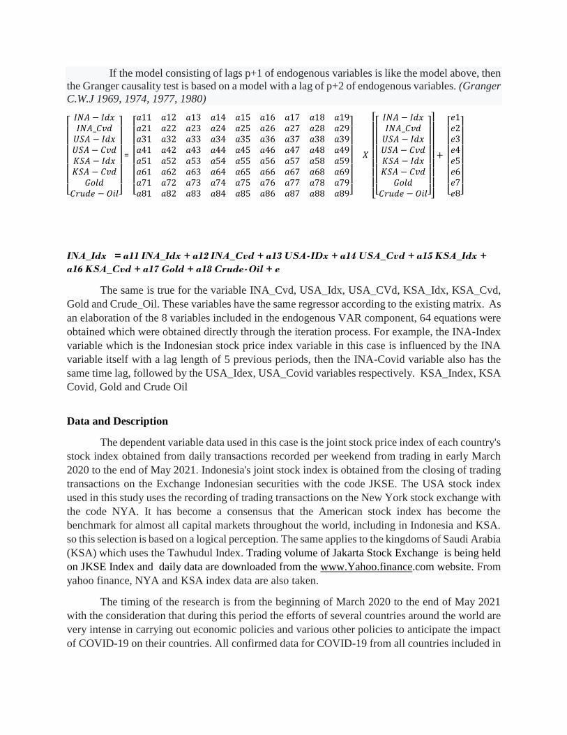
If the model consisting of lags p+1 of endogenous variables is like the model above, then
the Granger causality test is based on a model with a lag of p+2 of endogenous variables. (Granger
C.W.J 1969, 1974, 1977, 1980)
[
𝐼𝑁𝐴 − 𝐼𝑑𝑥𝐼𝑁𝐴_𝐶𝑣𝑑𝑈𝑆𝐴 − 𝐼𝑑𝑥𝑈𝑆𝐴 − 𝐶𝑣𝑑𝐾𝑆𝐴 − 𝐼𝑑𝑥𝐾𝑆𝐴 − 𝐶𝑣𝑑
𝐺𝑜𝑙𝑑𝐶𝑟𝑢𝑑𝑒 − 𝑂𝑖𝑙]
=
[ 𝑎11 𝑎12 𝑎13 𝑎14 𝑎15 𝑎16 𝑎17 𝑎18 𝑎19𝑎21 𝑎22 𝑎23 𝑎24 𝑎25 𝑎26 𝑎27 𝑎28 𝑎29𝑎31 𝑎32 𝑎33 𝑎34 𝑎35 𝑎36 𝑎37 𝑎38 𝑎39𝑎41 𝑎42 𝑎43 𝑎44 𝑎45 𝑎46 𝑎47 𝑎48 𝑎49𝑎51 𝑎52 𝑎53 𝑎54 𝑎55 𝑎56 𝑎57 𝑎58 𝑎59𝑎61 𝑎62 𝑎63 𝑎64 𝑎65 𝑎66 𝑎67 𝑎68 𝑎69𝑎71 𝑎72 𝑎73 𝑎74 𝑎75 𝑎76 𝑎77 𝑎78 𝑎79𝑎81 𝑎82 𝑎83 𝑎84 𝑎85 𝑎86 𝑎87 𝑎88 𝑎89]
𝑋
[
[
𝐼𝑁𝐴 − 𝐼𝑑𝑥𝐼𝑁𝐴_𝐶𝑣𝑑𝑈𝑆𝐴 − 𝐼𝑑𝑥𝑈𝑆𝐴 − 𝐶𝑣𝑑𝐾𝑆𝐴 − 𝐼𝑑𝑥𝐾𝑆𝐴 − 𝐶𝑣𝑑
𝐺𝑜𝑙𝑑𝐶𝑟𝑢𝑑𝑒 − 𝑂𝑖𝑙]
]
+
[ 𝑒1𝑒2𝑒3𝑒4𝑒5𝑒6𝑒7𝑒8]
INA_Idx = a11 INA_Idx + a12 INA_Cvd + a13 USA-IDx + a14 USA_Cvd + a15 KSA_Idx +
a16 KSA_Cvd + a17 Gold + a18 Crude-Oil + e
The same is true for the variable INA_Cvd, USA_Idx, USA_CVd, KSA_Idx, KSA_Cvd,
Gold and Crude_Oil. These variables have the same regressor according to the existing matrix. As
an elaboration of the 8 variables included in the endogenous VAR component, 64 equations were
obtained which were obtained directly through the iteration process. For example, the INA-Index
variable which is the Indonesian stock price index variable in this case is influenced by the INA
variable itself with a lag length of 5 previous periods, then the INA-Covid variable also has the
same time lag, followed by the USA_Idex, USA_Covid variables respectively. KSA_Index, KSA
Covid, Gold and Crude Oil
Data and Description
The dependent variable data used in this case is the joint stock price index of each country's
stock index obtained from daily transactions recorded per weekend from trading in early March
2020 to the end of May 2021. Indonesia's joint stock index is obtained from the closing of trading
transactions on the Exchange Indonesian securities with the code JKSE. The USA stock index
used in this study uses the recording of trading transactions on the New York stock exchange with
the code NYA. It has become a consensus that the American stock index has become the
benchmark for almost all capital markets throughout the world, including in Indonesia and KSA.
so this selection is based on a logical perception. The same applies to the kingdoms of Saudi Arabia
(KSA) which uses the Tawhudul Index. Trading volume of Jakarta Stock Exchange is being held
on JKSE Index and daily data are downloaded from the www.Yahoo.finance.com website. From
yahoo finance, NYA and KSA index data are also taken.
The timing of the research is from the beginning of March 2020 to the end of May 2021
with the consideration that during this period the efforts of several countries around the world are
very intense in carrying out economic policies and various other policies to anticipate the impact
of COVID-19 on their countries. All confirmed data for COVID-19 from all countries included in

this study were obtained from the Johns Hopkins University Covid-19 center which is also
affiliated with data at the World Health Organization (WHO).
EMPIRICAL RESULTS
Statistic descriptive
INA_INDEX USA_INDEX KSA_INDEX GOLD
Mean 5436.439 13509.29 29.89918 1806.864
Median 5304.500 13185.50 29.95451 1816.500
Maximum 6373.000 16708.00 39.24000 2010.000
Minimum 4195.000 9133.000 21.44511 1484.000
Std. Dev. 613.4961 1903.841 4.420635 105.3921
Skewness -0.016308 -0.056555 0.268885 -0.595139
Kurtosis 1.664482 2.082330 2.373219 3.458156
Jarque-Bera 4.907847 2.351007 1.875641 4.473335
Probability 0.085956 0.308664 0.391480 0.106814
Sum 358805.0 891613.0 1973.346 119253.0
Sum Sq. Dev. 24464538 2.36E+08 1270.231 721987.8
Observations 66 66 66 66
INA_COVID USA_COVID KSA_COVID CRUDE_OIL
Mean 27518.41 499232.8 6824.788 44.96045
Median 27069.50 367336.5 3422.000 41.28500
Maximum 90052.00 1753319. 28957.00 69.23000
Minimum 2.000000 20.00000 1.000000 16.94000
Std. Dev. 22450.18 435877.2 7242.887 13.52552
Skewness 0.789016 1.360235 1.565598 -0.035969
Kurtosis 3.161975 3.748660 4.690845 2.274784
Jarque-Bera 6.920155 21.89399 34.82420 1.460561
Probability 0.031427 0.000018 0.000000 0.481774
Sum 1816215. 32949366 450436.0 2967.390
Sum Sq. Dev. 3.28E+10 1.23E+13 3.41E+09 11891.08
Observations 66 66 66 66
Prior to examining the results from panel structural VAR, it is useful to consider the
trajectory of global financial markets and capital flows in the aftermath of the COVID-19 outbreak
It can be seen that government bond yields initially declined globally given rising uncertainty
amidst a bleak economic outlook, suggesting that investors considered sovereign bonds as safe
haven assets at the time. On Black Monday (9 March 2020), financial markets panicked over the
worsening of the COVID-19 pandemic and the concomitant oil price war between Saudi Arabia

and the Russian Federation. Stock markets tanked, while bond yields spiked. In compiling the
VAR structure, steps were made by Christopher Sim and Granger, who were pioneers in compiling
VAR in the mid-1980s. The consistency of these two economists in economics and the
methodology they work with, has led them both to get the prestigious Nobel Prize. The stages of
VAR can be seen in Appendixes 1 to 4.
Vector Autoregression Estimates
Date: 06/10/21 Time: 22:39
Sample (adjusted): 3/16/2020 5/31/2021
Included observations: 64 after adjustments
Standard errors in ( ) & t-statistics in [ ] INA_INDEX USA_INDEX KSA_INDEX GOLD INA_INDEX(-1) 0.499199 0.104049 -0.001156 0.043568
(0.21437) (0.60231) (0.00107) (0.06065)
[ 2.32863] [ 0.17275] [-1.07646] [ 0.71832]
INA_INDEX(-2) -0.234701 -0.274442 -0.000527 -0.071435
(0.20826) (0.58513) (0.00104) (0.05892)
[-1.12696] [-0.46903] [-0.50492] [-1.21237]
INA_COVID(-1) -0.003486 -0.000386 3.26E-05 7.71E-05
(0.00428) (0.01204) (2.1E-05) (0.00121)
[-0.81357] [-0.03208] [ 1.51825] [ 0.06361]
INA_COVID(-2) 0.007967 0.011293 -2.38E-05 -0.000114
(0.00386) (0.01083) (1.9E-05) (0.00109)
[ 2.06624] [ 1.04239] [-1.23209] [-0.10480]
USA_INDEX(-1) 0.003634 0.222617 0.000655 -0.063778
(0.08401) (0.23604) (0.00042) (0.02377)
[ 0.04325] [ 0.94311] [ 1.55770] [-2.68319]
USA_INDEX(-2) 0.106049 0.271562 0.000470 0.027997
(0.08472) (0.23802) (0.00042) (0.02397)
[ 1.25182] [ 1.14092] [ 1.10756] [ 1.16810]
USA_COVID(-1) 0.000559 0.000536 1.33E-06 2.56E-05
(0.00022) (0.00061) (1.1E-06) (6.1E-05)
[ 2.58084] [ 0.87980] [ 1.22527] [ 0.41719]
USA_COVID(-2) -0.000248 -0.000238 -1.79E-06 1.65E-05
(0.00024) (0.00069) (1.2E-06) (6.9E-05)
[-1.01395] [-0.34630] [-1.46277] [ 0.23832]
KSA_INDEX(-1) 70.75988 357.9212 0.893512 13.07208
(35.7918) (100.562) (0.17923) (10.1264)
[ 1.97698] [ 3.55922] [ 4.98538] [ 1.29089]
KSA_INDEX(-2) -92.46659 -178.1962 -0.363054 4.435994
(39.0206) (109.634) (0.19539) (11.0399)
[-2.36968] [-1.62538] [-1.85805] [ 0.40181]
KSA_COVID(-1) 0.004216 0.003958 1.22E-05 -0.005911
(0.00982) (0.02758) (4.9E-05) (0.00278)
[ 0.42947] [ 0.14351] [ 0.24866] [-2.12829]
KSA_COVID(-2) -0.005008 0.004896 -4.61E-05 0.007304
(0.01041) (0.02925) (5.2E-05) (0.00295)
[-0.48105] [ 0.16738] [-0.88483] [ 2.47958]
GOLD(-1) 0.692224 1.628000 0.004816 0.775988
(0.47027) (1.32130) (0.00235) (0.13305)
[ 1.47196] [ 1.23212] [ 2.04518] [ 5.83218]
GOLD(-2) -0.841024 -1.879444 -0.004773 -0.025049
(0.45646) (1.28247) (0.00229) (0.12914)
[-1.84251] [-1.46549] [-2.08812] [-0.19396]
CRUDE_OIL(-1) 0.485628 -3.758131 0.021290 -0.393287
(10.5720) (29.7035) (0.05294) (2.99110)
[ 0.04594] [-0.12652] [ 0.40216] [-0.13149]
CRUDE_OIL(-2) 12.53310 7.881672 0.036947 0.918412
(9.56798) (26.8825) (0.04791) (2.70703)
[ 1.30990] [ 0.29319] [ 0.77116] [ 0.33927]
C 2578.881 2209.152 5.705730 517.2791
(865.151) (2430.76) (4.33222) (244.773)
[ 2.98084] [ 0.90883] [ 1.31705] [ 2.11330] R-squared 0.962769 0.968692 0.980995 0.883041
Adj. R-squared 0.950094 0.958034 0.974525 0.843225
Sum sq. resids 900179.9 7106046. 22.57182 72056.49
S.E. equation 138.3935 388.8348 0.693002 39.15504
F-statistic 75.96099 90.88821 151.6240 22.17808
Log likelihood -396.4590 -462.5744 -57.46228 -315.6544
Akaike AIC 12.92059 14.98670 2.326946 10.39545
Schwarz SC 13.49405 15.56015 2.900400 10.96890
Mean dependent 5443.719 13568.89 30.09108 1813.531
S.D. dependent 619.4978 1898.085 4.341850 98.88922 Determinant resid covariance (dof adj.)
Determinant resid covariance
Log likelihood
-3299.192
Akaike information criterion 107.3
497
Schwarz criterion 111.9
374
Number of coefficients 136
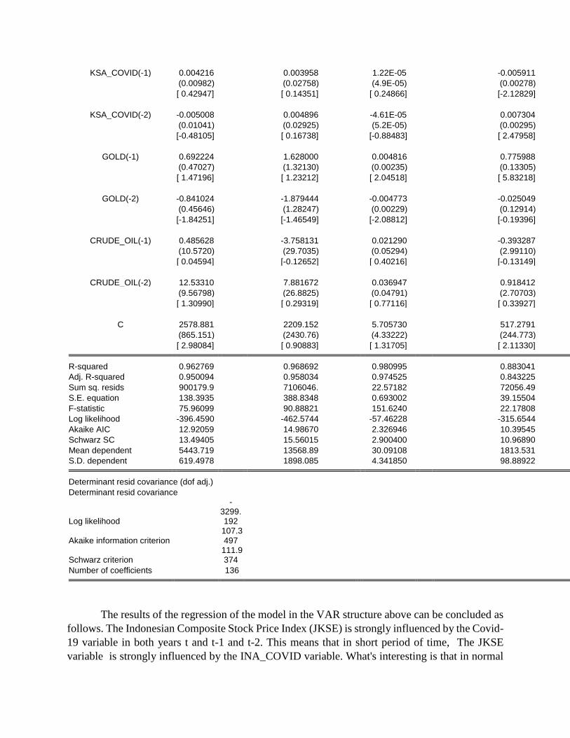
The results of the regression of the model in the VAR structure above can be concluded as
follows. The Indonesian Composite Stock Price Index (JKSE) is strongly influenced by the Covid-
19 variable in both years t and t-1 and t-2. This means that in short period of time, The JKSE
variable is strongly influenced by the INA_COVID variable. What's interesting is that in normal

situations, usually JKSE or INA_INDEX is strongly influenced by the performance of the New
York Stock Exchange, which in this case is a pooling of top US companies that are members of
the Fortune 500. In the period of this study the USA_INDEX variable can be said to be significant
if the t test enlarged to 10%. This means that the NYSE does not have a strong influence on the
JKSE with a 5% probability test. The same thing also happened to the variable Gold and Crude
Oil. Both did not significantly affect the JKSE and NYSE indexes. In normal situations, Gold and
Crude Oil indicators are usually very significant in influencing both the INA_Index and
USA_Index variables. For the KSA index, the results of the regression in the VAR structure are
still strongly influenced by the USA index more than other variables. This is understandable
considering the strong inter-relationship between US and KSA interests in terms of investment and
other matters.
4,400
4,800
5,200
5,600
6,000
6,400
I II III IV I II
2020 2021
INA_INDEX_F
20
24
28
32
36
40
I II III IV I II
2020 2021
KSA_INDEX_F
9,000
10,000
11,000
12,000
13,000
14,000
15,000
16,000
17,000
I II III IV I II
2020 2021
USA_INDEX_F
Forecast Evaluation
Date: 06/10/21 Time: 22:44
Sample: 3/02/2020 5/31/2021
Included observations: 66

Variable Inc. obs. RMSE MAE MAPE Theil CRUDE_OIL 66 4.405371 3.374577 8.014188 0.046013
GOLD 66 84.76001 70.61182 3.829458 0.023231
INA_COVID 66 14754.25 10447.45 53.14936 0.217533
INA_INDEX 66 274.1048 224.0758 4.044083 0.024977
KSA_COVID 66 5043.723 3930.315 58.68300 0.283428
KSA_INDEX 66 1.344173 1.004067 3.159258 0.021795
USA_COVID 66 405750.4 299846.3 88.54880 0.343269
USA_INDEX 66 451.0506 336.0296 2.522196 0.016297 RMSE: Root Mean Square Error
MAE: Mean Absolute Error
MAPE: Mean Absolute Percentage Error
Theil: Theil inequality coefficient
Figure 1 shows the dynamics of expected Index growth expectations in the Indonesia, US
and KSA respectively. Growth expectations did not respond much to Country lockdown such in
Italy, Germany, UK and France. For Example, the lockdown in Italy, is followed by growth
expectations start to deteriorate). The travel restrictions on visitors to the US from the EU leads to
a sharp deterioration of growth expectations. This is occurs once again following the declaration
of the national emergency and the subsequent actions by the Federal Reserve on March 15.
Following the US fiscal stimulus program, GDP growth has stabilized somewhat in the US but
continued to deteriorate in the EU. By June 8, expected dividend growth over the next year is down
by 9% for the S&P 500 index and 14% for the Euro Stoxx 50 index. The estimate of GDP growth
over the next year is down by 2.0% in the US and 3.1% in the EU. As a word of caution, we
emphasize that these estimates are based on a forecasting model estimated using historical data. In
these unprecedented times, there is a risk that the historical relation between growth and asset
prices changes, meaning these estimates come with uncertainty. Nevertheless, in discussing what
asset markets may tell about investors’ growth expectations, we argue that dividend futures should
play a central role. (Gormsen and Koijen, 2020)
The policies carried out by Indonesia in the midst of the COVID-19 pandemic were met
with pros and cons, considering that the sectors affected by the pandemic actually rose on autopilot.
The government's policies that are felt to be directly related to the lower class are not clearly
visible. Once again, Indonesia has a unique social character and can be a role model for the world.
The nature of the community that works together is the mainstay of the community to get out of
the crisis turmoil due to the pandemic. We can see that during the pandemic, people provide food
assistance to low-income people, such as online motorcycle taxis, scavengers and other poor
people. This is what makes Indonesia resistant to the COVID-19 pandemic whose impact is very
massive and is felt by almost all elements of society.

Conclusion and Discussion
Looking at the structure of the equations compiled in the VAR model, it can be concluded
that both the Indonesia Composite Stock Index (JKSE) and the NYSE are strongly influenced by
Covid-19 data, in the form of confirmed COVID-19 patients. Surprisingly, the indicators of world
oil and world gold prices which have so far greatly influenced both the NYSE and JKSE, in the
period of this research, from March 1, 2020 to May 31, 2021, do not have a significant influence
on the two indices above.
The theoretical implication that can be drawn from the regression results above is that it
is true that Covid-19 is the main determining indicator in the pandemic era, especially in the
research period (March 2020 to May 2021). Once again, the opinion of many economists who call
Covid-19 a black swan phenomenon is understandable, considering that no one can predict when
it will occur and how long it will last. But one thing that can be learned is that, when the worst
condition occurs, the prediction of the long run will get better. This is what is happening at this
time, where conditions that were not previously thought have occurred, other things that are
remarkable or beyond human reasoning can happen.
.
The managerial implication of this research is very important for monetary and financial
policy makers both in the US and Indonesia, namely the momentum of providing fiscal stimulus
to the poor. cash transfer is the best way to deal with the pandemic that affects the middle to lower
economy. on the other hand, the covid-19 pandemic for financial investors, especially the capital
market, can be used as a honeymoon event in stock trading. how not, the very deep fall of stock
exchange trading is always followed by a rebound in either the short or medium term. In the midst
of the Covid-19 pandemic, many investors actually gained very large gains when collecting stocks
that fell at the beginning of the pandemic.
Referrences
Alber, N. (2020 ). “The Effect of Coronavirus Spread on Stock Markets: The Case of the Worst 6
Countries,” Available at: http://ssrn.com/abstract=3578080
Alber, N. & Saleh, A. (2020). “The Impact of Covid-19 Spread on Stock Markets: The Case of the
GCC Countries," International Business Research 13 (11)
Beirne, J, Renzhi N, Sugandi E, and Volz Ulrich, “Financial Market and Capital Flow Dynamics
During The Covid-19 Pandemic“ ADBI Working Paper Series
Eom, T.H. and Rubenstein, R. 2006. Do state-funded property tax exemptions increase local
government inefficiency? An analysis of New York State’s STAR Program, Public Budgeting &
Finance, 26(1): 66–87
Eom, T.H , Lee S.H , and Hua Xu , “Introduction to Panel Data Analysis: Concepts and Practices”
, Hanyang University of China
Gujarati, D.N. 2003. Basic Econometrics, 4th ed., New York: McGraw Hill.
Wooldridge, J.M. 2006. Introductory Econometrics: A Modern Approach, 3rd ed., Mason, Ohio:
Thomson South-Wester
Granger, C. W. J. (1969). Investigating Causal Relations by Econometric Models and Cross-
Spectral Methods. Econometrica, 37, 424-38.
Granger, C. W. J. and Newbold, P. (1974). "Spurious regressions in econometrics". Journal of
Econometrics 2 (2): 111–120
Granger, C. W. J. and Newbold, P. (1977). Forecasting Economic Time Series. Academic Press
Granger C.W.J. (1980) “Testing for Causality - A Personal Viewpoint”, Journal of Economic
Dynamics and Control, 2, 329-52
Heckman, J.J. 2000. Casual parameters and policy analysis in economics: A twentieth century
retrospective, The Quarterly Journal of Economics, 115(1): 45–97.
Heckman, J.J. 2001. Micro data, heterogeneity and the evaluation of public policy: Nobel lecture,
Journal of Political Economy, 109(4): 673–748
Lucas, R. 1976. The Phillips curve and labor market, in Carnegie-Rochester Conference Series on
Public Policy, K. Brunner and A.H. Meltzer (Eds.), North-Holland Publishing Company.
Maddala, G.S. 2001. Introduction to Econometrics, 3rd ed., New York: John Wiley & Sons
Ramelli, Stefano and Alexander F. Wagner. 2020. Feverish Stock Price Reactions to COVID-19.
Swiss Finance Institute Research Paper Series No. 20-12. Zurich: Swiss Finance Institute
Sims, C.A (1982), “Policy Analysis with Econometric Models”, Brooking Papers on Economic
Activity, 107-64
Zaremba Adam, Kizysc R , Tzouvanasd P, Aharone David Y , and Demir E, “The Quest for
Multidimensional Financial Immunity to the COVID-19 Pandemic: Evidence from International
Stock Markets”, SSRN.com
Thakur, S. (2020). “Effect of COVID-19 on Capital Market with Reference to S&P 500,”
Available at: SSRN 3640871
Alber, N, Refaat (2020) The Effects of Covid-19 Spread on the Egyptian Exchange Sectors:
Winners and Losers across Time : http://ssrn.com/abstract=3741179

Gormsen, N.J and Koijen, R.S.J, “Coronavirus: Impact on Stock Prices and Growth Expectation”
Working Paper 27387 http://www.nber.org/papers/w27387, NBER Working Paper Series
National Bureau of Economic Research 1050 Massachusetts Avenue Cambridge, MA 02138 June
2020
Appendix 1. Computing Unit Root
Null Hypothesis: INA_INDEX has a unit root
Exogenous: Constant
Lag Length: 0 (Automatic - based on SIC, maxlag=10) t-Statistic Prob.* Augmented Dickey-Fuller test statistic -0.925908 0.7739
Test critical values: 1% level -3.534868
5% level -2.906923
10% level -2.591006 *MacKinnon (1996) one-sided p-values.
Augmented Dickey-Fuller Test Equation
Dependent Variable: D(INA_INDEX)
Method: Least Squares
Date: 06/11/21 Time: 07:20
Sample (adjusted): 3/09/2020 5/31/2021
Included observations: 65 after adjustments Variable Coefficient Std. Error t-Statistic Prob. INA_INDEX(-1) -0.033471 0.036150 -0.925908 0.3580
C 190.3485 197.4051 0.964253 0.3386 R-squared 0.013425 Mean dependent var 8.707692
Adjusted R-squared -0.002235 S.D. dependent var 177.1323
S.E. of regression 177.3301 Akaike info criterion 13.22419
Sum squared resid 1981097. Schwarz criterion 13.29109
Log likelihood -427.7862 Hannan-Quinn criter. 13.25059
F-statistic 0.857305 Durbin-Watson stat 1.529181
Prob(F-statistic) 0.358027
Appendix 2. Computing Stationary
Null Hypothesis: D(INA_INDEX) has a unit root
Exogenous: Constant
Lag Length: 0 (Automatic - based on SIC, maxlag=10) t-Statistic Prob.* Augmented Dickey-Fuller test statistic -7.636764 0.0000
Test critical values: 1% level -3.536587
5% level -2.907660
10% level -2.591396

*MacKinnon (1996) one-sided p-values.
Augmented Dickey-Fuller Test Equation
Dependent Variable: D(INA_INDEX,2)
Method: Least Squares
Date: 06/11/21 Time: 07:21
Sample (adjusted): 3/16/2020 5/31/2021
Included observations: 64 after adjustments Variable Coefficient Std. Error t-Statistic Prob. D(INA_INDEX(-1)) -0.879147 0.115120 -7.636764 0.0000
C 17.41721 20.17856 0.863154 0.3914 R-squared 0.484708 Mean dependent var 12.60938
Adjusted R-squared 0.476397 S.D. dependent var 222.9809
S.E. of regression 161.3499 Akaike info criterion 13.03578
Sum squared resid 1614096. Schwarz criterion 13.10324
Log likelihood -415.1449 Hannan-Quinn criter. 13.06236
F-statistic 58.32017 Durbin-Watson stat 2.141562
Prob(F-statistic) 0.000000
Appendix 3 Computing AR Root Graph
-1.5
-1.0
-0.5
0.0
0.5
1.0
1.5
-1.5 -1.0 -0.5 0.0 0.5 1.0 1.5
Inverse Roots of AR Characteristic Polynomial
Appendix 4. Granger Causality Test
VEC Granger Causality/Block Exogeneity Wald Tests

Date: 06/11/21 Time: 11:30
Sample: 3/02/2020 5/31/2021
Included observations: 60
Dependent variable: D(INA_INDEX,2) Excluded Chi-sq df Prob. D(INA_COVID,2) 14.05388 4 0.0071
D(USA_INDEX,2) 5.561590 4 0.2344
D(USA_COVID,2) 24.12999 4 0.0001
D(KSA_INDEX,2) 10.41048 4 0.0341
D(KSA_COVID,2) 0.806225 4 0.9376
D(GOLD) 16.06977 4 0.0029
D(CRUDE_OIL) 3.980824 4 0.4086 All 77.51796 28 0.0000
Dependent variable: D(INA_COVID,2) Excluded Chi-sq df Prob. D(INA_INDEX,2) 5.857322 4 0.2101
D(USA_INDEX,2) 3.480870 4 0.4808
D(USA_COVID,2) 8.592531 4 0.0721
D(KSA_INDEX,2) 2.529026 4 0.6394
D(KSA_COVID,2) 0.336255 4 0.9874
D(GOLD) 1.343464 4 0.8540
D(CRUDE_OIL) 2.861125 4 0.5813 All 35.24525 28 0.1628
Dependent variable: D(USA_INDEX,2) Excluded Chi-sq df Prob. D(INA_INDEX,2) 8.612173 4 0.0716
D(INA_COVID,2) 7.019992 4 0.1348
D(USA_COVID,2) 6.206789 4 0.1842
D(KSA_INDEX,2) 2.120195 4 0.7137
D(KSA_COVID,2) 1.964788 4 0.7422
D(GOLD) 5.678326 4 0.2245
D(CRUDE_OIL) 5.380007 4 0.2505 All 30.44673 28 0.3422
Dependent variable: D(USA_COVID,2) Excluded Chi-sq df Prob. D(INA_INDEX,2) 5.140453 4 0.2732
D(INA_COVID,2) 14.80365 4 0.0051
D(USA_INDEX,2) 7.101568 4 0.1306

D(KSA_INDEX,2) 1.381230 4 0.8475
D(KSA_COVID,2) 1.795747 4 0.7733
D(GOLD) 5.238392 4 0.2637
D(CRUDE_OIL) 0.759088 4 0.9438 All 37.70108 28 0.1042
Dependent variable: D(KSA_INDEX,2) Excluded Chi-sq df Prob. D(INA_INDEX,2) 6.665887 4 0.1546
D(INA_COVID,2) 10.65305 4 0.0308
D(USA_INDEX,2) 6.232408 4 0.1825
D(USA_COVID,2) 1.567931 4 0.8145
D(KSA_COVID,2) 0.919798 4 0.9217
D(GOLD) 3.953907 4 0.4123
D(CRUDE_OIL) 1.116784 4 0.8916 All 23.45882 28 0.7098
Dependent variable: D(KSA_COVID,2) Excluded Chi-sq df Prob. D(INA_INDEX,2) 11.44653 4 0.0220
D(INA_COVID,2) 4.468796 4 0.3463
D(USA_INDEX,2) 12.56446 4 0.0136
D(USA_COVID,2) 2.850433 4 0.5832
D(KSA_INDEX,2) 5.056394 4 0.2816
D(GOLD) 4.549962 4 0.3367
D(CRUDE_OIL) 4.563563 4 0.3351 All 35.32102 28 0.1607
Dependent variable: D(GOLD) Excluded Chi-sq df Prob. D(INA_INDEX,2) 1.892150 4 0.7556
D(INA_COVID,2) 4.439357 4 0.3498
D(USA_INDEX,2) 1.228818 4 0.8733
D(USA_COVID,2) 1.907682 4 0.7527
D(KSA_INDEX,2) 4.113663 4 0.3908
D(KSA_COVID,2) 3.365413 4 0.4986
D(CRUDE_OIL) 3.791164 4 0.4350 All 35.84425 28 0.1466
Dependent variable: D(CRUDE_OIL) Excluded Chi-sq df Prob.

D(INA_INDEX,2) 8.989068 4 0.0614
D(INA_COVID,2) 10.57935 4 0.0317
D(USA_INDEX,2) 12.48598 4 0.0141
D(USA_COVID,2) 14.00376 4 0.0073
D(KSA_INDEX,2) 13.66354 4 0.0085
D(KSA_COVID,2) 6.680530 4 0.1538
D(GOLD) 6.741651 4 0.1502 All 46.51023 28 0.0154
Appendix 5 Computing Vector Error Correction Estimates
Vector Error Correction Estimates
Date: 06/11/21 Time: 07:42
Sample (adjusted): 4/13/2020 5/31/2021
Included observations: 60 after adjustments
Standard errors in ( ) & t-statistics in [ ] Cointegrating Eq: CointEq1 D(INA_INDEX(-1)) 1.000000
D(INA_COVID(-1)) -0.004278
(0.00275)
[-1.55516]
D(USA_INDEX(-1)) -0.411914
(0.07452)
[-5.52773]
D(USA_COVID(-1)) -0.000570
(9.5E-05)
[-5.99133]
D(KSA_INDEX(-1)) 128.2346
(28.6396)
[ 4.47753]
D(KSA_COVID(-1)) -0.044520
(0.00602)
[-7.39269]
GOLD(-1) -0.185750
(0.10814)
[-1.71765]
CRUDE_OIL(-1) -0.330587
(0.35746)
[-0.92482]
C 358.4305
Error Correction: D(INA_INDEX,2
) D(INA_COVID,2
) D(USA_INDEX,
2) D(USA_COVID,
2) D(KSA_INDEX,
2) D(KSA_COVID,
2) D(GOLD)
CointEq1 -0.459760 -9.851813 0.026818 214.1004 0.000450 13.61081 0.035190
(0.26658) (15.5655) (1.01239) (252.908) (0.00188) (5.57646) (0.10056)
[-1.72465] [-0.63293] [ 0.02649] [ 0.84655] [ 0.23920] [ 2.44076] [ 0.34994]
D(INA_INDEX(-1),2) -0.178490 9.887500 0.889750 110.0932 -0.000289 -13.27963 0.024876
(0.29879) (17.4461) (1.13470) (283.464) (0.00211) (6.25019) (0.11271)
[-0.59738] [ 0.56675] [ 0.78413] [ 0.38839] [-0.13715] [-2.12468] [ 0.22071]
D(INA_INDEX(-2),2) -0.444075 25.08028 -0.921437 -109.3139 -0.002999 -2.855132 0.085968
(0.26904) (15.7092) (1.02173) (255.243) (0.00190) (5.62794) (0.10149)
[-1.65058] [ 1.59654] [-0.90184] [-0.42827] [-1.58001] [-0.50731] [ 0.84708]
D(INA_INDEX(-3),2) -0.300502 25.22817 -0.854984 -129.4585 -0.002479 -0.779739 0.031254
(0.24241) (14.1544) (0.92061) (229.981) (0.00171) (5.07092) (0.09144)
[-1.23962] [ 1.78236] [-0.92872] [-0.56291] [-1.44916] [-0.15377] [ 0.34179]
D(INA_INDEX(-4),2) -0.061064 7.003296 -0.791783 110.5377 -0.001568 2.760428 0.039147
(0.15882) (9.27353) (0.60316) (150.676) (0.00112) (3.32231) (0.05991)
[-0.38448] [ 0.75519] [-1.31273] [ 0.73361] [-1.39939] [ 0.83087] [ 0.65342]
D(INA_COVID(-1),2) -0.008052 -0.915699 -0.004941 -2.068600 1.21E-05 0.070245 0.000906
(0.00297) (0.17344) (0.01128) (2.81810) (2.1E-05) (0.06214) (0.00112)
[-2.71078] [-5.27955] [-0.43796] [-0.73404] [ 0.57818] [ 1.13048] [ 0.80855]
D(INA_COVID(-2),2) -0.007457 -0.441884 0.003155 -6.737800 -1.85E-05 0.070886 0.002370
(0.00370) (0.21631) (0.01407) (3.51459) (2.6E-05) (0.07749) (0.00140)
[-2.01280] [-2.04284] [ 0.22423] [-1.91709] [-0.70736] [ 0.91473] [ 1.69591]
D(INA_COVID(-3),2) -0.011793 0.042285 -0.025975 -12.21955 -7.74E-05 0.152347 0.002952
(0.00387) (0.22623) (0.01471) (3.67582) (2.7E-05) (0.08105) (0.00146)
[-3.04364] [ 0.18691] [-1.76532] [-3.32430] [-2.83072] [ 1.87969] [ 2.01956]
D(INA_COVID(-4),2) -0.005512 0.181754 -0.008787 -10.72762 -5.36E-05 0.065640 0.001237
(0.00325) (0.18999) (0.01236) (3.08690) (2.3E-05) (0.06806) (0.00123)
[-1.69405] [ 0.95667] [-0.71108] [-3.47521] [-2.33692] [ 0.96438] [ 1.00815]
D(USA_INDEX(-1),2) -0.162376 -9.405475 -0.717225 137.5702 0.000623 4.447029 -0.007633
(0.12836) (7.49459) (0.48745) (121.772) (0.00091) (2.68500) (0.04842)
[-1.26505] [-1.25497] [-1.47137] [ 1.12973] [ 0.68784] [ 1.65625] [-0.15765]
D(USA_INDEX(-2),2) -0.076438 -12.51801 -0.340764 182.2184 0.001288 3.818032 -0.027043
(0.12938) (7.55465) (0.49136) (122.748) (0.00091) (2.70651) (0.04881)
[-0.59078] [-1.65699] [-0.69351] [ 1.48449] [ 1.41123] [ 1.41068] [-0.55409]
D(USA_INDEX(-3),2) -0.114378 -11.07602 -0.353818 72.71588 0.000663 4.439482 -0.019855
(0.12003) (7.00838) (0.45583) (113.872) (0.00085) (2.51081) (0.04528)
[-0.95293] [-1.58040] [-0.77621] [ 0.63857] [ 0.78257] [ 1.76815] [-0.43852]
D(USA_INDEX(-4),2) -0.106034 -4.836037 0.046594 -9.416914 0.000148 0.544684 -0.014174
(0.07678) (4.48297) (0.29158) (72.8394) (0.00054) (1.60606) (0.02896)
[-1.38105] [-1.07876] [ 0.15980] [-0.12928] [ 0.27403] [ 0.33914] [-0.48940]
D(USA_COVID(-1),2) 7.46E-05 0.022713 0.000729 -0.411552 5.91E-07 0.003700 8.19E-05
(0.00020) (0.01173) (0.00076) (0.19052) (1.4E-06) (0.00420) (7.6E-05)
[ 0.37142] [ 1.93705] [ 0.95651] [-2.16021] [ 0.41734] [ 0.88089] [ 1.08082]

D(USA_COVID(-2),2) -0.000162 0.021072 0.000471 -0.439413 8.92E-07 0.001078 5.07E-05
(0.00022) (0.01279) (0.00083) (0.20781) (1.5E-06) (0.00458) (8.3E-05)
[-0.74142] [ 1.64757] [ 0.56581] [-2.11453] [ 0.57687] [ 0.23533] [ 0.61398]
D(USA_COVID(-3),2) 0.000182 0.017195 0.001598 0.241994 2.00E-06 -0.002558 1.00E-05
(0.00025) (0.01433) (0.00093) (0.23276) (1.7E-06) (0.00513) (9.3E-05)
[ 0.74208] [ 1.20034] [ 1.71486] [ 1.03968] [ 1.15458] [-0.49833] [ 0.10841]
D(USA_COVID(-4),2) 0.000660 0.027094 0.001489 0.381120 1.10E-06 -0.000395 -9.29E-06
(0.00020) (0.01139) (0.00074) (0.18509) (1.4E-06) (0.00408) (7.4E-05)
[ 3.38399] [ 2.37853] [ 2.00930] [ 2.05916] [ 0.80241] [-0.09687] [-0.12623]
D(KSA_INDEX(-1),2) 70.90091 6014.759 -106.3397 -63433.40 -1.049828 -2312.722 -30.32159
(69.2756) (4044.96) (263.086) (65722.5) (0.48878) (1449.14) (26.1319)
[ 1.02346] [ 1.48698] [-0.40420] [-0.96517] [-2.14787] [-1.59593] [-1.16033]
D(KSA_INDEX(-2),2) 81.84985 6122.056 -132.3758 -47703.89 -1.013504 -2750.904 -26.85711
(71.9551) (4201.41) (273.262) (68264.5) (0.50768) (1505.19) (27.1426)
[ 1.13751] [ 1.45714] [-0.48443] [-0.69881] [-1.99634] [-1.82762] [-0.98948]
D(KSA_INDEX(-3),2) 0.863698 4702.259 -215.9304 -49367.92 -0.803860 -2155.685 -34.89441
(65.9110) (3848.50) (250.309) (62530.5) (0.46504) (1378.75) (24.8627)
[ 0.01310] [ 1.22184] [-0.86266] [-0.78950] [-1.72859] [-1.56350] [-1.40348]
D(KSA_INDEX(-4),2) 40.88320 3006.763 -47.70380 -35343.86 -0.116606 -874.0523 -7.532492
(44.3510) (2589.62) (168.431) (42076.2) (0.31292) (927.753) (16.7299)
[ 0.92181] [ 1.16108] [-0.28323] [-0.84000] [-0.37264] [-0.94212] [-0.45024]
D(KSA_COVID(-1),2) -0.008108 -0.055797 -0.007146 12.30112 4.50E-05 0.010780 -0.004402
(0.01144) (0.66825) (0.04346) (10.8578) (8.1E-05) (0.23941) (0.00432)
[-0.70848] [-0.08350] [-0.16441] [ 1.13293] [ 0.55759] [ 0.04503] [-1.01964]
D(KSA_COVID(-2),2) -0.007541 -0.198028 0.006653 12.10061 5.83E-05 -0.212137 -0.005592
(0.01117) (0.65237) (0.04243) (10.5997) (7.9E-05) (0.23372) (0.00421)
[-0.67492] [-0.30355] [ 0.15680] [ 1.14160] [ 0.73911] [-0.90767] [-1.32673]
D(KSA_COVID(-3),2) -0.007737 -0.055877 -0.014282 5.863222 2.83E-05 0.176189 -0.006227
(0.00913) (0.53281) (0.03465) (8.65710) (6.4E-05) (0.19088) (0.00344)
[-0.84786] [-0.10487] [-0.41213] [ 0.67727] [ 0.43999] [ 0.92302] [-1.80912]
D(KSA_COVID(-4),2) -0.004684 0.059535 0.028093 6.360987 4.85E-05 -0.047921 -0.002927
(0.00797) (0.46533) (0.03027) (7.56077) (5.6E-05) (0.16671) (0.00301)
[-0.58773] [ 0.12794] [ 0.92821] [ 0.84131] [ 0.86175] [-0.28745] [-0.97371]
D(GOLD(-1)) 0.634102 17.61648 0.644470 388.0502 0.001387 -8.371264 -0.163895
(0.46392) (27.0882) (1.76183) (440.130) (0.00327) (9.70456) (0.17500)
[ 1.36682] [ 0.65034] [ 0.36579] [ 0.88167] [ 0.42367] [-0.86261] [-0.93655]
D(GOLD(-2)) -0.948509 21.91701 -1.267944 -556.3714 0.000368 -3.446925 0.066093
(0.39390) (22.9998) (1.49592) (373.702) (0.00278) (8.23987) (0.14859)
[-2.40796] [ 0.95292] [-0.84760] [-1.48881] [ 0.13233] [-0.41832] [ 0.44481]
D(GOLD(-3)) 1.039519 4.167195 3.730438 380.2367 0.005910 -4.226477 -0.044800
(0.48602) (28.3785) (1.84575) (461.094) (0.00343) (10.1668) (0.18334)
[ 2.13883] [ 0.14684] [ 2.02109] [ 0.82464] [ 1.72345] [-0.41571] [-0.24436]
D(GOLD(-4)) 0.760407 3.716705 -1.129962 -448.8828 -0.002304 17.43608 0.148333

(0.45752) (26.7143) (1.73752) (434.055) (0.00323) (9.57062) (0.17258)
[ 1.66202] [ 0.13913] [-0.65033] [-1.03416] [-0.71379] [ 1.82183] [ 0.85948]
D(CRUDE_OIL(-1)) -5.187147 -378.1723 -14.41469 5681.778 0.068346 348.1718 -0.262931
(11.9125) (695.562) (45.2398) (11301.5) (0.08405) (249.191) (4.49359)
[-0.43544] [-0.54369] [-0.31863] [ 0.50275] [ 0.81317] [ 1.39721] [-0.05851]
D(CRUDE_OIL(-2)) 7.827794 -645.0067 55.97923 -2764.454 0.025979 -70.73245 1.653109
(9.51398) (555.515) (36.1310) (9026.01) (0.06713) (199.017) (3.58883)
[ 0.82277] [-1.16110] [ 1.54934] [-0.30628] [ 0.38702] [-0.35541] [ 0.46063]
D(CRUDE_OIL(-3)) 9.743638 336.5220 20.71735 -874.1859 0.027793 -75.85999 3.427928
(7.45507) (435.296) (28.3119) (7072.70) (0.05260) (155.948) (2.81218)
[ 1.30698] [ 0.77309] [ 0.73175] [-0.12360] [ 0.52839] [-0.48644] [ 1.21896]
D(CRUDE_OIL(-4)) -4.953048 364.6796 -29.34248 -3938.372 -0.032274 -210.9002 -4.126178
(7.36298) (429.919) (27.9622) (6985.33) (0.05195) (154.022) (2.77744)
[-0.67270] [ 0.84825] [-1.04936] [-0.56381] [-0.62126] [-1.36929] [-1.48561]
C -4.416970 467.1706 -37.51750 -1237.626 -0.086136 -180.8658 1.910721
(19.7031) (1150.45) (74.8259) (18692.5) (0.13902) (412.158) (7.43233)
[-0.22418] [ 0.40608] [-0.50140] [-0.06621] [-0.61962] [-0.43883] [ 0.25708] R-squared 0.867120 0.735784 0.779988 0.748854 0.705761 0.707113 0.607680
Adj. R-squared 0.698464 0.400433 0.500742 0.430092 0.332303 0.335371 0.109736
Sum sq. resids 254772.8 8.69E+08 3674418. 2.29E+11 12.68271 1.11E+08 36252.21
S.E. equation 98.98967 5779.937 375.9306 93912.50 0.698424 2070.708 37.34054
F-statistic 5.141351 2.194071 2.793192 2.349254 1.889803 1.902162 1.220377
Log likelihood -335.7498 -579.7778 -415.8131 -747.0560 -38.51317 -518.1876 -277.2536
Akaike AIC 12.32499 20.45926 14.99377 26.03520 2.417106 18.40625 10.37512
Schwarz SC 13.51179 21.64605 16.18057 27.22200 3.603901 19.59305 11.56192
Mean dependent 3.166667 54.61667 -18.40000 -1446.400 0.020978 0.216667 2.566667
S.D. dependent 180.2686 7464.560 532.0409 124400.1 0.854732 2539.973 39.57502 Determinant resid covariance (dof adj.) 8.55E+34
Determinant resid covariance 1.06E+32
Log likelihood -2893.406
Akaike information criterion 105.7802
Schwarz criterion 115.5538
Number of coefficients 280
Appendix 6 Computing Variance Decomposition Response of D(INA_INDE
X):
Period D(INA_INDEX) D(INA_COVID
) D(USA_INDE
X) D(USA_COVI
D) D(KSA_INDEX
) D(KSA_COVI
D) GOLD CRUDE_OIL 1 98.98967 0.000000 0.000000 0.000000 0.000000 0.000000 0.000000 0.000000
2 49.45153 -26.30335 -7.810547 30.20432 1.532832 19.09187 26.30534 -3.501568
3 27.72653 -22.03783 35.58754 -16.77782 -0.286402 17.82375 -33.17091 11.02614
4 4.457314 -53.07925 -8.991869 -2.998671 -12.19831 11.41768 27.16427 7.516554
5 -4.359242 -7.071244 -32.80648 46.64739 -17.98768 1.486360 22.63976 0.119222
6 70.84426 -19.79412 -4.268301 -13.09778 -21.33004 11.64507 7.911950 -3.473559
7 31.48940 -4.984444 16.86227 3.831054 -16.77485 19.30294 -20.27434 -1.783494

8 16.83715 -18.31931 -17.98915 17.10362 -17.54224 9.086136 -3.466365 2.474385
9 18.51897 -7.896582 -25.87376 32.07039 -13.28068 25.59127 16.73677 2.591561
10 38.60658 6.311310 6.223579 21.49672 -4.555450 14.58229 26.14716 -2.038612 Response of
D(INA_COVID):
Period D(INA_INDEX) D(INA_COVID
) D(USA_INDE
X) D(USA_COVI
D) D(KSA_INDEX
) D(KSA_COVI
D) GOLD CRUDE_OIL 1 -1800.185 5492.450 0.000000 0.000000 0.000000 0.000000 0.000000 0.000000
2 -314.9097 1504.280 -931.4226 2729.391 1568.605 456.2125 721.3783 -260.7251
3 301.0283 2764.171 -1407.822 983.0111 -307.5509 251.5137 952.4648 52.32383
4 530.5834 1458.357 -981.2296 2050.128 206.6670 475.9949 999.1415 -122.4837
5 -543.4798 1112.584 -1026.559 3028.070 353.0645 399.7043 624.3685 198.8450
6 700.9566 -474.3921 -1776.845 -255.1029 -606.5822 -75.13076 363.8520 166.4615
7 -995.5395 1500.129 -619.5294 2074.459 334.6182 -377.5088 1031.759 -215.4095
8 -150.7427 166.9968 -1384.725 1620.233 -309.9686 72.79468 337.3816 73.93642
9 495.0050 1541.154 -886.5811 468.0150 -632.0882 179.5857 124.9503 -199.4616
10 -795.8729 1650.629 -187.4129 1148.269 252.7977 -393.9166 863.4495 -63.01491 Response of
D(USA_INDEX):
Period D(INA_INDEX) D(INA_COVID
) D(USA_INDE
X) D(USA_COVI
D) D(KSA_INDEX
) D(KSA_COVI
D) GOLD CRUDE_OIL 1 192.7350 -32.94661 321.0787 0.000000 0.000000 0.000000 0.000000 0.000000
2 107.0264 -42.42410 0.565089 66.50213 -65.20298 -25.48855 23.81349 -10.03048
3 -27.05895 -33.03215 145.3217 15.50883 13.59436 50.17921 -25.02795 32.19051
4 -24.27254 -160.1361 29.29039 42.64645 -18.59153 -23.53614 90.05184 22.61676
5 34.28563 1.897322 60.68001 67.50617 -75.09873 0.015135 -26.97027 -12.25588
6 163.9966 -90.66125 113.5400 17.75650 -7.958789 -14.52302 -21.66167 -0.666976
7 53.62550 -77.20970 113.3626 -13.21992 -65.79428 22.09275 -50.38934 5.027681
8 43.28242 -81.42569 107.4141 15.76213 -20.01635 -1.346498 -38.65736 -2.342825
9 -13.60274 -25.14228 80.49715 60.24792 -19.00572 21.89540 8.629999 20.27523
10 98.55721 -37.84344 98.07431 25.62058 -10.05321 -10.81655 13.80352 -4.694000 Response of
D(USA_COVID):
Period D(INA_INDEX) D(INA_COVID
) D(USA_INDE
X) D(USA_COVI
D) D(KSA_INDEX
) D(KSA_COVI
D) GOLD CRUDE_OIL 1 -13247.33 6493.065 -30729.66 87507.69 0.000000 0.000000 0.000000 0.000000
2 29035.92 -16723.67 -9365.844 35626.79 -7806.145 8316.195 12382.62 3902.023
3 33464.99 -46366.84 -2507.139 24188.62 -11328.53 2561.553 -10264.20 -2929.425
4 -1813.474 -61976.66 -17668.61 38099.77 -11878.68 -6039.852 -17279.18 4976.808
5 4552.917 -61649.89 -36570.74 34057.02 -21427.56 -889.5595 -16452.23 6138.958
6 21928.65 -26701.73 15141.14 13065.53 -5598.889 -10164.13 -1644.348 -6476.774
7 27817.76 -44396.26 14490.55 2362.657 -7086.285 -10357.85 -40867.07 -2347.748
8 9062.370 -35836.35 -8638.397 16209.67 -11707.99 -4617.110 -23157.44 1022.841
9 -3761.824 -24829.33 -12546.37 31197.67 -7402.053 -7132.994 937.8663 1429.655
10 25918.44 -20981.37 12832.90 16263.13 9425.271 -6697.770 -12977.35 -3333.181 Response of
D(KSA_INDEX):

Period D(INA_INDEX) D(INA_COVID
) D(USA_INDE
X) D(USA_COVI
D) D(KSA_INDEX
) D(KSA_COVI
D) GOLD CRUDE_OIL 1 0.281789 0.056669 0.490094 0.020713 0.405659 0.000000 0.000000 0.000000
2 0.077588 0.049452 0.215845 -0.014467 0.092388 0.088350 0.044277 0.047426
3 -0.034482 -0.158274 0.190025 0.079499 0.047237 0.061873 0.051132 0.007861
4 -0.015790 -0.316208 0.036310 -0.042207 0.007655 -0.059933 0.081779 0.047544
5 0.055573 -0.051818 0.154436 -0.081893 0.135331 -0.016775 -0.046564 0.008864
6 0.102191 0.105821 0.332646 -0.018542 0.173363 -0.003739 -0.047831 -0.002989
7 0.122266 -0.130702 0.242377 -0.093753 0.063010 0.034490 -0.082854 -0.007862
8 0.046812 -0.061023 0.228823 -0.073734 0.099213 0.000682 -0.012812 0.010641
9 -0.062438 -0.019006 0.169543 0.037862 0.147960 0.036776 0.077342 0.044535
10 0.092538 0.048595 0.217004 0.004205 0.155851 0.020281 -0.008169 0.005995 Response of
D(KSA_COVID):
Period D(INA_INDEX) D(INA_COVID
) D(USA_INDE
X) D(USA_COVI
D) D(KSA_INDEX
) D(KSA_COVI
D) GOLD CRUDE_OIL 1 284.0102 506.0426 -509.0173 3.403477 435.3719 1871.478 0.000000 0.000000
2 -129.6248 248.7495 -282.8506 -527.4750 403.1001 987.8968 -410.1415 238.9979
3 536.2512 216.2720 -422.2190 -617.0190 118.1008 76.02689 -227.7351 -38.77020
4 967.2674 637.8612 50.24104 -420.0015 385.6363 786.5755 -342.6636 -171.8151
5 562.3763 324.8364 -450.4118 -328.6220 562.6251 581.4962 114.5603 -57.08032
6 -94.26371 158.1385 -91.06531 -535.3461 294.0960 400.3598 244.2974 157.0076
7 201.9416 329.5722 -318.4534 -311.6277 155.8784 229.4554 577.2904 -36.02595
8 358.6103 344.3594 -717.8319 -339.9889 281.8765 190.6121 244.2707 -48.97138
9 431.4028 108.4291 -369.0477 -614.5994 597.4611 109.1571 247.0663 40.01470
10 107.0561 341.6766 -104.5241 -409.0156 265.5916 398.7213 288.7982 12.51206 Response of
GOLD:
Period D(INA_INDEX) D(INA_COVID
) D(USA_INDE
X) D(USA_COVI
D) D(KSA_INDEX
) D(KSA_COVI
D) GOLD CRUDE_OIL 1 -6.880423 -2.025249 1.570559 -3.433652 -3.569057 -1.189939 36.25553 0.000000
2 -15.17248 -0.864247 -17.68436 2.164605 -16.36305 -12.33084 30.08840 -0.190938
3 -12.50082 3.361784 -20.63454 5.522425 -14.13253 -17.34234 36.75998 -1.571686
4 -17.87360 8.479488 -22.44995 6.313248 -13.51194 -16.49757 35.42208 -0.025988
5 -11.50962 10.59700 -19.76127 13.06505 -8.868854 -16.00353 40.44525 -4.185692
6 -17.34681 4.623280 -20.04849 17.39614 -14.99784 -9.041405 39.09682 0.757155
7 -17.35592 2.015135 -26.35093 19.56757 -20.05556 -9.214221 44.72077 -0.367309
8 -17.98187 0.539104 -27.19908 17.50041 -21.32294 -9.952269 39.48172 -0.079386
9 -16.27042 0.140588 -27.78502 15.58374 -17.31977 -10.15637 36.02909 -0.746684
10 -17.18108 4.785824 -27.51197 19.37826 -19.94298 -7.738204 34.57244 -0.926749 Response of
CRUDE_OIL:
Period D(INA_INDEX) D(INA_COVID
) D(USA_INDE
X) D(USA_COVI
D) D(KSA_INDEX
) D(KSA_COVI
D) GOLD CRUDE_OIL 1 -0.003423 -0.069564 1.355635 -0.579736 1.216564 0.632315 -0.043574 0.695424
2 -0.082267 0.346242 1.109252 -0.569795 1.467462 0.791907 0.451243 0.550311
3 -0.438123 0.111353 1.488298 -0.613299 1.525466 1.149203 -0.355909 0.587892
4 -0.682408 -0.527378 1.355642 -0.803465 1.212519 1.481709 -0.211446 0.743303
5 -0.936840 -0.094421 1.021693 -0.408996 0.712121 1.783625 -0.248000 0.617014

6 -0.576236 0.594782 1.407108 -0.596963 0.851556 1.941100 -0.579708 0.531730
7 -0.508072 0.795619 1.388974 -0.739981 0.889946 2.185281 -1.060009 0.570517
8 -0.619070 1.168904 1.008854 -0.188434 0.859018 2.193433 -0.768706 0.473176
9 -0.478098 1.112726 0.750393 0.300039 0.820421 2.384724 -0.546148 0.499383
10 -0.050046 0.953757 0.936771 0.202156 0.904377 2.353287 -0.458290 0.498852 Cholesky Ordering: D(INA_INDEX) D(INA_COVID) D(USA_INDEX) D(USA_COVID) D(KSA_INDEX) D(KSA_COVID)
GOLD
CRUDE_OIL