Spectrum Sharing Between A Surveillance Radar … Sharing Between A Surveillance Radar and Secondary Wi-Fi Networks ... Abstract Co-existence between ... and 3100-3650 MHz for military

Spectrum Sharing Between A Surveillance

Radar and Secondary Wi-Fi NetworksFarzad Hessar, Student Member, IEEE, Sumit Roy, Fellow, IEEE,

Electrical Engineering Department, University of Washington

farzad, [email protected]

Abstract

Co-existence between unlicensed networks that share spectrum spatio-temporally with terrestrial (e.g. Air Traffic

Control) and shipborne radars1 in 3 GHz band is attracting significant interest. Similar to every primary-secondary

coexistence scenario, interference from unlicensed devices to a primary receiver must be within acceptable bounds. In

this work, we formulate the spectrum sharing problem between a pulsed, search radar (primary) and 802.11 WLAN

as the secondary. We compute the protection region for such a search radar for a) a single secondary user (initially) as

well as b) a random spatial distribution of multiple secondary users. Furthermore, we also analyze the interference to

the WiFi devices from the radar’s transmissions to estimate the impact on achievable WLAN throughput as a function

of distance to the primary radar.

Index Terms

Spectrum Sharing, Coexistence, Opportunistic Spectrum Access, Radar, Unlicensed Spectrum, Cognitive Networks

I. INTRODUCTION

Wireless data traffic has been increasing exponentially over the last decade, resulting from the boom in multimedia

applications running on high-end client devices such as smart phones, tablets [1]. Various solutions are suggested

for expanding capacity of wireless networks, from higher spectral efficiency to smaller cell sizes; utilizing additional

spectrum is always a major element of the solution. The scarcity of available new RF spectrum and technological

limitations for usage of higher frequency bands (above 60 GHz) has led to a renewed emphasis on more efficient

use of existing spectrum. This has motivated spectrum regulatory bodies such as FCC (US) and Ofcom (UK) to

promulgate dynamic access rules by smart secondary devices. This allows cognitive secondary users to detect locally

unused white spaces and use them for a period, subject to agreed upon rules of primary protection [2], [3].

Contact Author: [email protected]

This work was supported in part by AFRL via Task CRFR-009-02-01 and NSF AST 14439231In the US, airport radars are allocated 2700-2900 MHz, and 3100-3650 MHz for military radar operations for national defense.

arX

iv:1

602.

0080

2v1

[cs

.IT

] 2

Feb

201

6

2

In this work, we focus on spectrum sharing between primary radar systems and secondary 802.11 WLAN networks

- a topic on which little work exists beyond the studies in [4]–[13]. The re-emergence of interest in this topic is

based in part on large amount of licensed spectrum allocated to radar operations in the U.S. - over 1700 MHz in

225 MHz to 3.7 GHz band, are set aside for radar and radio-navigation [14] and the widespread deployment of

802.11 WLAN networks. Given that terrestrial radar locations are fixed and have predictable operational patterns, it

is possible to model their behavior and utilize it for a database-driven coexistence solution, akin to the architecture

espoused by the FCC for TV white spaces [15].

Database-driven spectrum sharing uses a geo-location database that determines available spectrum for a secondary

user (SU) requesting access based on their location. This coexistence mechanism is currently mandated by the FCC

for operation in UHF TV bands; its main impact was to remove the burden of spectrum sensing from secondary

devices thereby simplifying receiver design for clients and also avoiding other challenges in distributed spectrum

sensing such as the well-known hidden terminal problem. By rules of cognitive access, overlay secondary users

are prohibited from re-using a primary operating channel within an area defined as the protection region. The geo-

location database has access to relevant information of primary users such as location, transmit power, interference

tolerance, etc. that it utilizes to estimate this protection region to enable any secondary transmitter to meet the

interference protection conditions.

The actual implementation of any incumbent protection rule depends strongly on the usage scenario, i.e., features

of the primary and secondary systems and the consequent co-existence requirements. In this paper, we consider

a rotating search radar as the licensed transmitter and WiFi networks as unlicensed devices. First, we review

the known design equations that represent performance characteristics of a typical search radar for the purely

noise limited case in terms of the desired probability of detection PD and false alarm PFA. This determines the

minimum SNR requirements at the boundary of the radar operating range and sets the baseline for comparison with

any spectrum sharing regime.

In order to permit overlay transmission by secondaries, we need to define the rules for co-existence. A recent

program suggests drop of 5% in PD for fixed PFA [5] at the edge of radar operating range as being acceptable;

this defines the protection regime for the primary receiver (from secondary interference). However, the fundamental

objective of any WS type spectrum sharing scenario is to promote secondary usage subject to the primary protection

constraints; we thus also analyze the effect of (high power) radar pulse sequences on the throughput of WiFi

network. Any successful spectrum sharing system must balance the rights of the incumbent (primary protection)

with encouraging new services, and we hope that our work fundamentally highlights the inherent trade-offs in this

design space.

A. Related Works

There is growing interest in radar spectrum sharing from both regulators and researchers [4]–[13], [16]–[23].

SSPARC program from DARPA [5] is a good example that seeks to support two types of sharing: a) Mili-

tary/military sharing between military radars and military communication systems to increase capabilities of both

February 3, 2016 DRAFT

3

and b) Military/commercial sharing between military radars and commercial communication systems to preserve

radar capabilities while meeting the need for increased capacity of commercial networks.

In [6]–[8], the authors study coexistence between radar and a cellular base station. The co-existence strategy

espoused is variable secondary transmit power assuming a maximum tolerable interference at the radar. Further,

the authors consider only one sharing scenario in which SU is perfectly synchronized with radar rotation (a very

impractical assumption). The limitations of this analysis is thus apparent - it does not explore at any depth, how the

radar’s interference tolerance is determined based on the system parameters and geometry considerations. Similarly

in [4], temporal variations of radar antenna’s main lobe is exploited to support more white space users when their

location is not within the main lobe. In [9], spectrum sensing is combined with database approach to create a hybrid

spectrum sharing technique. The authors in [12] study the potential for secondary LTE usage in 2.7-2.9 GHz radar

bands for different scenarios such as home eNodeB (HeNB) at street levels or in high-rise buildings, macro LTE

transmitters and so on. A fixed Interference-to-Noise ratio (INR) of -10 dB is specified for sharing without any

discussion on radar performance. The analysis does not consider radar rotation and mostly focused on single-user

sharing with radar. While the case of multiple SU is considered, it is done so under an unrealistic assumption that

all users are at the same distance from radar. Finally, spectrum sharing between a MIMO radar and a wireless

communication system is analyzed in [13]. Their interference mitigation approach is shown to eliminate wireless

interferences from main/side lobe while maintaining target detection performance.

Some U.S. DoD studies for co-existence with radars operating in the 2700-2900 MHz and 5250-5850 MHz

bands [18], [19] have also been conducted. Protection criteria against external interference is determined through

experimental measurements by injecting three types of unwanted communications waveform emissions - continuous

wave, CDMA-QPSK, and TDMA-QPSK. In [20], the authors evaluate interference from broadband communication

transmitters such as WiMax to WSR-88D next-generation weather radar (2700-2900 MHz). A computation model

for calculating aggregate interference from radio local area networks to 5-GHz radar systems is provided in [21].

The analysis methodology is based on using point to point path loss models between radio networks and radar as

well as other link parameters such as antenna gains and frequency-dependent rejection [16], [17].

Our major contribution in this work is a complete characterization of Radar - WiFi coexistence as a function of all

relevant system parameters and design constraints/objectives. First, the maximum tolerable interference from WiFi

networks to radar is estimated for both a a) single WiFi network and b) a (random) spatial distribution of multiple

WiFi networks. Depending on how much information about radar is available to secondary (WiFi) networks, various

sharing scenarios are considered, resulting in different protection distances. Second,the (time-varying) interference

from radar to WiFi networks is modeled and achievable secondary link throughput is estimated.

The rest of this paper is organized as follows. In section II, baseline performance for a noise limited radar is

formulated. Section III considers coexistence between radar and a single SU. Multiple SU with spatial distribution

is discussed in IV. In section V, interference from radar to SU is studied as a limiting factor to available white

space capacity. Numerical results are provided in VI and finally VII concludes the paper.


4

II. SEARCH RADAR: NOISE LIMITED OPERATION [24]

We first review operational characteristics of a typical search radar in the noise limited regime with no external

source of interference. For a radar transmitting a pulse train x(t) =∑n

√PT s(t− n

fR) with instantaneous power

PT and pulse repetition frequency of fR, the power of reflected signal from the target at the radar receiver, assuming

free space propagation is given by the well-know Radar Equation, i.e.,

PR =PTG

2λ2

(4π)3d4σ (1)

where G is the radar’s antenna gain (relative to isotropic antenna) on both transmit and receive, λ is the wavelength

and d the distance from source to the target of interest, and σ represents the target’s radar cross section.

For a single received pulse, the signal-to-noise ratio (SNR) at the receiver input is calculated as

SNRp =PTG

2λ2

(4π)3d4N0fBWσ (2)

with fBW representing the pulse bandwidth and N0 being the one-sided noise spectral density.

N0 = FKTE (3)

where F is the receiver noise figure and TE is the ambient temperature. Radar detection typically operates based

on processing of multiple pulses received from the target. For a coherent radar receiver that uses M pulses, the

energy of the pulses are integrated such that the resulting SNR at the detector input is increased by a factor of M ,

i.e.,

SNReff = MPTG

2λ2

(4π)3d4N0fBWσ (4)

where M = TI fR, product of illumination time TI and pulse repetition frequency fR. The target illumination

time TI depends on radar scan rate as well as antenna pattern. Let θV and θH (in radian) denote the vertical and

horizontal antenna beam width, respectively, then the antenna gain can be approximated as

G ≈ 4π

θHθVρA (5)

where ρA is the antenna efficiency, i.e., the radar antenna is concentrating an otherwise uniformly distributed power

into an area of θV θH with efficiency of ρA where the latter is typically around 0.5. If radar is scanning over an

area of Ω (steradians), within a scan time of TS , then illumination time is determined as:

TI ≈ TSθHθV

Ω≈ TS

4πρAΩG

(6)

For a radar that searches the entire azimuth/elevation plane, Ω = 4π.

Using (4)-(6) yields

SNReff =TSΩ

PTGλ2fR

(4π)2d4N0fBWLσ (7)

Here, antenna efficiency ρA is replaced by L that represents total losses in the system, including antenna efficiency,

transmission lines mismatch, perfect coherence in pulse detector, etc.


5

A. Minimum Required SNR

Radar detection performance is defined in terms of two probabilities, detection PD and false alarm PFA, which

in turn depend on SNR at the detector input. The latter is determined by the pulse integration method that is utilized

by the receiver, namely coherent versus non-coherent.

a) Single pulse, hard detection: If the received signal at the detector input is

e0(t) = r(t) cos (ωct+ φ(t)) (8)

then the PDF of the detected envelope for a single pulse is Rician, i.e.,

p(r) =r

β2e

−(r2+A2)

2β2 I0

(rA

β2

)(9)

where A is the amplitude of the base band pulse and β =√N0fBW . Therefore, PFA is determined by setting

A = 0 and integrating over 0 to detection threshold VT as:

PFA = e−V 2

T2β2 (10)

A similar general closed-form equation for PD is complicated. However, for high-SNR cases, p(r) is well approx-

imated as Gaussian, for which case PD is given by [24]

PD =1

2

[1− erf

(VT

β√

2−√

SNRp

)](11)

The relationship between PD, PFA and SNR is fairly accurately expressed via the following empirical equation

[24]:

SNRp = ln

(0.62

PFA

)+ 0.12 ln

(0.62

PFA

)ln

(PD

1− PD

)+ 1.7 ln

(PD

1− PD

)(12)

b) Coherent Integrator: For a coherent receiver integrating M pulses, the SNR-performance relationship is

described in (12) in which SNRp should be replaced with the effective SNR at the detector input (SNReff),

determined by (7).

c) Noncoherent Integrator: If radar utilizes a linear (rather than square-law) detector for single pulse and then

combines M pulses non-coherently, the required SNR per pulse for desired PD, PFA is [25]:

SNRp,dB = −5 log10(M) +

[6.2 +

4.54√M + 0.44

]log10(A+ 0.12AB + 1.7B)

A = ln0.62

PFA, B = ln

PD1− PD

(13)

Overall, the baseline performance of a noise-limited radar can be evaluated in two ways:

• Assuming that maximum operational range of the radar is known, calculate SNR from (2) or (7) for the

maximum distance d. Then, using either (12) or (13), we can trade-off between PD and PFA.

• Assuming that target PD and PFA is specified, estimate required SNR from (12) or (13) and then determine

maximum range from (2) or (7).

For our calculations in the following sections, we consider a detector with coherent integration, using effective SNR

in (7) with (12).


6

III. INTERFERENCE LIMITED RADAR - SINGLE SECONDARY

In this section, we consider spectrum sharing with a single Wi-Fi user as the secondary device by treating

secondary signals as an external interference to radar receiver. Wi-Fi transmissions use OFDM signals, whereby

each OFDM symbol is a linear combination of many randomly modulated sub-carriers. Hence, using central limit

theorem, each sample of OFDM signal in time-domain is well-approximated as a Gaussian random variable. The

matched filter utilized at radar front-end for pulse detection applies another linear transformation on this OFDM

signal and results in a Gaussian random variable which is independent of AWGN (thermal noise) at the radar

receiver [26]. Therefore, the interference power can be directly added to AWGN noise power, effectively raising

the noise floor. Thus system performance is determined by Signal-to-Interference-plus-Noise ratio (SINR) at radar

receiver input. Using (7), this is given by

SINR =TSΩ

PTGλ2fR

(4π)2d4L (N0fBW + I)σ (14)

where I represents total interference power received from secondary user. The latter depends on various factors:

the distance and frequency dependent path loss between secondary source and radar receiver, the azimuth between

SU direction and radar’s main antenna beam, etc. as below:

ISU→Radar =PSUG(αH , αV )

L1(dRd−SU )FDR(∆f)(15)

where G(αH , αV ) defines radar’s antenna gain in the direction of SU (considering azimuth and elevation), FDR(∆f)

is frequency dependent rejection factor that depends on spectral shape of transmitted signal P (f) and receiver receive

input filter H(f), i.e.

FDR(∆f) =

∫∞0P (f)df∫∞

0P (f)H(f + ∆f)df

(16)

represents the out-of-band emission from the WiFi source into the radar RF receiver front-end as a function of

∆f = ft − fr, the difference between interferer and receiver tuned center frequency. For a special case of exact

co-channel operation ∆f = 0; for a perfectly flat filter response H(f) = 1, FDR simplifies as the ratio of WiFi to

radar bandwidth:

FDR = max

(WiFi BWfBW

, 1

)(17)

Our focus in this paper is cases where radar bandwidth is less than WiFi bandwidth, FDR ≥ 1.

The minimum required SINR for normal operation of the radar was defined in previous section. Therefore

maximum additional interference level I that can be tolerated is determined as:

SINR0 ≤TSΩ

PTGλ2fRσ

(4π)2d4L (N0fBW + I)

I ≤ TSΩ

PTGλ2fRσ

(4π)2d4LSINR0−N0fBW = Imax (18)


7

Using (15) and (18), we can calculate the minimum separation distance between radar and SU2 as:

dRd−SU ≥ L−1Rd−SU

(PSUG(αH , αV )

FDR(∆f)Imax

)(19)

Where LRd−SU (.) is the path-loss between radar and SU as a function distance. As this equation suggests, the

minimum separation distance depends on the instantaneous antenna gain, G(αH , αV ).

A. Numerical Results

For the computations in this section, we use radar parameters from ITU document, Rec. ITU-R M.1464-1, for

a typical aeronautical radio-navigation radar in 2.8 GHz band. Table VI in Appendix provides parameters for the

so-called type-B radar in [18]. We choose performance points (of ROC) shown in Table I for the radar in noise

and interference limited cases. As suggested by SSPARC, a drop of 5% in performance is permitted to provide an

TABLE I

TARGET ROC FOR NOISE/INTERFERENCE LIMITED PERFORMANCE

Mode PD PFA SNR/SINR (dB)

Noise Limited 0.90 10−6 13.14

Interference Limited 0.85 10−6 12.80

interference margin for the secondary user, which is equivalent to an SNR loss of 0.34 dB.

To calculate max allowable interference level, Imax in (18), maximum operational range d and minimum target’s

radar cross section σ are required which is not provided by Table VI. Any variation in values of these two parameters

can significantly affect resulting Imax. For example, if the SNR of the noise-limited regime in (7) is 16.14 dB (3-dB

above the required SNR in table I) then Imax can be about as high as noise level N0fBW (INR of 0 dB), which

brings SINR down to 13.14 dB. However, if we assume that SNR is already at the minimum level, then we only

have 0.34 dB room for the interference which reduces the maximum INR down to −11 dB.

The type-B radar, as outlined in [18], employs high and low-beam horns in the antenna feed array. The high-beam

horn receives returns from high-altitude targets close to the antenna, while the low-beam horn receives returns from

low-altitude targets at greater distances. Overall, it is designed for monitoring air traffic in and around airports

within a range of 60 Nm (approximately 111 km). A coverage pattern is also provided for a target with 1 m2 radar

cross section. Therefore, using d = 111 km and σ = 1, the resulting SNR (7) will be 30.6 dB that is significantly

bigger than required SNR of 13.14 dB. This is unrealistic and does not represent radar’s borderline operation.

Therefore, in order to remove the effect of d and σ in our calculation, we normalize them such that SNR in (7)

matches with required SNR in (12)3. Based on these normalized parameter values, Table II shows the maximum

2Or equivalently maximum transmission power for a known distance3By increasing the value of d or decreasing σ, effective SNR is reduced to match with (12)


8

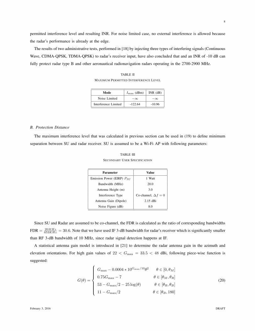
permitted interference level and resulting INR. For noise limited case, no external interference is allowed because

the radar’s performance is already at the edge.

The results of two administrative tests, performed in [18] by injecting three types of interfering signals (Continuous

Wave, CDMA-QPSK, TDMA-QPSK) to radar’s receiver input, have also concluded that and an INR of -10 dB can

fully protect radar type B and other aeronautical radionavigation radars operating in the 2700-2900 MHz.

TABLE II

MAXIMUM PERMITTED INTERFERENCE LEVEL

Mode Imax (dBm) INR (dB)

Noise Limited −∞ −∞

Interference Limited -122.64 -10.96

B. Protection Distance

The maximum interference level that was calculated in previous section can be used in (19) to define minimum

separation between SU and radar receiver. SU is assumed to be a Wi-Fi AP with following parameters:

TABLE III

SECONDARY USER SPECIFICATION

Parameter Value

Emission Power (EIRP) PSU 1 Watt

Bandwidth (MHz) 20.0

Antenna Height (m) 3.0

Interference Type Co-channel, ∆f = 0

Antenna Gain (Dipole) 2.15 dBi

Noise Figure (dB) 8.0

Since SU and Radar are assumed to be co-channel, the FDR is calculated as the ratio of corresponding bandwidths

FDR = 20MHz653KHz = 30.6. Note that we have used IF 3-dB bandwidth for radar’s receiver which is significantly smaller

than RF 3-dB bandwidth of 10 MHz, since radar signal detection happens at IF.

A statistical antenna gain model is introduced in [21] to determine the radar antenna gain in the azimuth and

elevation orientations. For high gain values of 22 < Gmax = 33.5 < 48 dBi, following piece-wise function is

suggested:

G(θ) =

Gmax − 0.0004 ∗ 10Gmax/10θ2 θ ∈ [0, θM ]

0.75Gmax − 7 θ ∈ [θM , θR]

53−Gmax/2− 25 log(θ) θ ∈ [θR, θB ]

11−Gmax/2 θ ∈ [θB , 180]

(20)


9

−150 −100 −50 0 50 100 150−10

0

10

20

30

40

RelativesAzimuths(degree)

Rad

arsA

nten

nasG

ains

(dB

i)

−150 −100 −50 0 50 100 150

10

20

30

40

50

Pro

tect

ions

Dis

tanc

es(k

m)

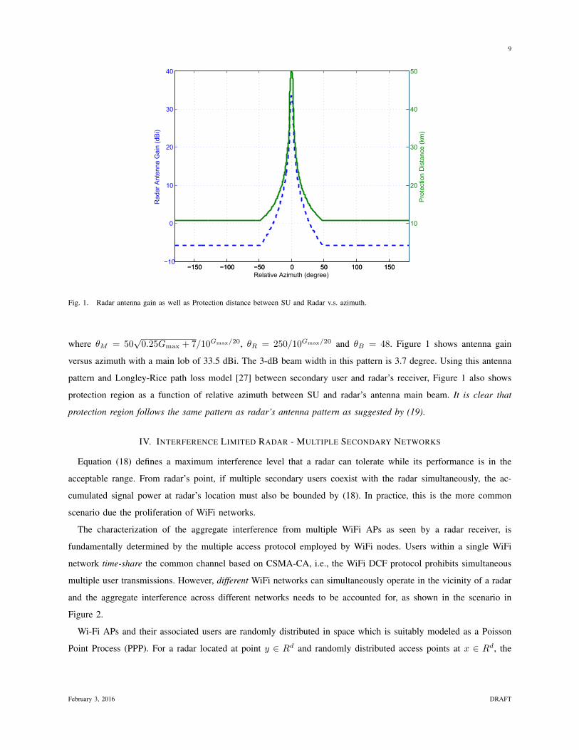
Fig. 1. Radar antenna gain as well as Protection distance between SU and Radar v.s. azimuth.

where θM = 50√

0.25Gmax + 7/10Gmax/20, θR = 250/10Gmax/20 and θB = 48. Figure 1 shows antenna gain

versus azimuth with a main lob of 33.5 dBi. The 3-dB beam width in this pattern is 3.7 degree. Using this antenna

pattern and Longley-Rice path loss model [27] between secondary user and radar’s receiver, Figure 1 also shows

protection region as a function of relative azimuth between SU and radar’s antenna main beam. It is clear that

protection region follows the same pattern as radar’s antenna pattern as suggested by (19).

IV. INTERFERENCE LIMITED RADAR - MULTIPLE SECONDARY NETWORKS

Equation (18) defines a maximum interference level that a radar can tolerate while its performance is in the

acceptable range. From radar’s point, if multiple secondary users coexist with the radar simultaneously, the ac-

cumulated signal power at radar’s location must also be bounded by (18). In practice, this is the more common

scenario due the proliferation of WiFi networks.

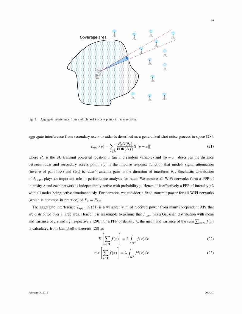
The characterization of the aggregate interference from multiple WiFi APs as seen by a radar receiver, is

fundamentally determined by the multiple access protocol employed by WiFi nodes. Users within a single WiFi

network time-share the common channel based on CSMA-CA, i.e., the WiFi DCF protocol prohibits simultaneous

multiple user transmissions. However, different WiFi networks can simultaneously operate in the vicinity of a radar

and the aggregate interference across different networks needs to be accounted for, as shown in the scenario in

Figure 2.

Wi-Fi APs and their associated users are randomly distributed in space which is suitably modeled as a Poisson

Point Process (PPP). For a radar located at point y ∈ Rd and randomly distributed access points at x ∈ Rd, the


10

Coverage area

Fig. 2. Aggregate interference from multiple WiFi access points to radar receiver.

aggregate interference from secondary users to radar is described as a generalized shot noise process in space [28]:

Iaggr(y) =∑x∈Φ

PxG(θx)

FDR(∆f)l(||y − x||) (21)

where Px is the SU transmit power at location x (an i.i.d random variable) and ||y − x|| describes the distance

between radar and secondary access point. l(.) is the impulse response function that models signal attenuation

(inverse of path loss) and G(.) is radar’s antenna gain in the direction of interferer, θx. Stochastic distribution

of Iaggr, plays an important role in performance analysis for radar. We assume all WiFi networks form a PPP of

intensity λ and each network is independently active with probability p. Hence, it is effectively a PPP of intensity pλ

with all nodes being active simultaneously. Furthermore, we consider a fixed transmit power for all WiFi networks

(which is common in practice) of Px = PSU .

The aggregate interference Iaggr in (21) is a weighted sum of received power from many independent APs that

are distributed over a large area. Hence, it is reasonable to assume that Iaggr has a Gaussian distribution with mean

and variance of µI and σ2I , respectively [29]. For a PPP of density λ, the mean and variance of the sum

∑x∈Φ f(x)

is calculated from Campbell’s theorem [28] as

E

[∑x∈Φ

f(x)

]= λ

∫Rd

f(x)dx (22)

var

[∑x∈Φ

f(x)

]= λ

∫Rd

f2(x)dx (23)


11

A. Average and Variance of Interference (µI , σ2I )

The average interference that is received at radar receiver is calculated from (22) by integrating over the R2

plane. Assuming that radar receiver is at the origin (y = 0):

µI = E[Iaggr] =pλPSU

FDR(∆f)

∫R2

G(θx)l(||x||)dx (24)

Here we assume there is a minimum separation distance between radar and SU which could potentially be a function

of θ, d(θ). Using polar coordinates for the integral and considering l(r) = K0r−α we obtain:

µI =pλPSUK0

FDR(∆f)

∫θ

∫ ∞d(θ)

G(θ)r1−αdrdθ = CµI

∫θ

G(θ)d2−α(θ)dθ

CµI =pλPSUK0

FDR(∆f)(α− 2)(25)

whenever α > 2 is necessary to guarantee convergence of inner integral. This excludes the ideal ‘free space’ (α = 2)

but holds for all practical scenarios of interest.

This equation allows variation in protection distance according to current direction of the radar’s main antenna

beam. The total interference highly depends on the choice of function d(θ) as a systematic parameter that trade-offs

protection distances between main beam interferer versus side lobe ones. This is clearly chosen based on G(θ) and

optimized subject to some constraints, as shown in the following sections.

The variance of aggregated interference is calculated from (23). Similar to the approach taken for µI , the variance

σ2I is calculated by the following double integral over r and θ:

σ2I =

pλP 2SUK

20

FDR2(∆f)

∫θ

∫ ∞d(θ)

G2(θ)r−αrdrdθ = Cσ2I

∫θ

G2(θ)d2−2α(θ)dθ

Cσ2I

=pλP 2

SUK20

FDR2(∆f)(2α− 2)(26)

with the assumption that α > 1 to ensure convergence of the integration over r.

B. Protection Region

With multiple secondary users being active simultaneously, protection region for radar can be defined in terms

of probability of outage, i.e. probability of effective radar SINR dropping below the minimum threshold. This is

also equivalent to limiting aggregate interference Iaggr < Imax. Since Iaggr has a normal distribution N(µI , σ2I ),

the outage probability can be determined as following:

Poutage = PrIaggr > Imax = Q

(Imax − µI

σI

)(27)

where Q(.) function is the tail probability of the standard normal distribution. It is desired to set an upper bound

for probability of outage, Pout,max:

Poutage ≤ Pout,max → Q

(Imax − µI

σI

)≤ Pout,max

Imax ≥ µI + σIQ−1 (Pout,max) (28)


12

This equation defines the relationship between maximum tolerable interference by the radar receiver and aver-

age/variance of aggregate interference from secondary WiFi networks. Depending on how much information about

radar rotation is available at the SU, different scenarios are plausible for determining protection distance d(θ). Here

we consider three special cases.

First: A secondary network that has full knowledge about current radar antenna beam position with respect to its

location.

Second, the case of a SU that has no knowledge about radar rotation pattern and therefore is not capable of

synchronizing its transmission instances with it. This results in a constant d(θ) = dmin and a circular protection

region.

Third, the case of secondary user that is partially aware of radar’s rotation schedule and is capable of identifying

radar’s main lobe from side lobe (representing a pragmatic, intermediate scenario between the above two).

Estimates of the protection distance is sensitive to the choice of the path loss model adopted. We use the well-

known Longley-Rice (L-R) model that is based on field measurements and is relatively more accurate. However,

previous analysis needs a closed form attenuation function of the form l(r) = K0r−α. Accordingly, we performed

exponential curve fitting on L-R with parameters in tables III and VI to estimate α and K0. L-R defines three

propagation regions, namely line of sight, diffraction and scattering. By using line-of-sight region for curve fitting,

l(r) = 259 r−3.97 is obtained.

1) Optimal Distance: Using (28), the coexistence criteria is defined by limiting average and variance of aggregate

interference µI+σIQ−1 (Pout,max) ≤ Imax. This inequality has a trivial answer that is achieved by letting d(θ)→∞

(apparent from (25) for example). In order to avoid this, we minimize the total protection area subject to net

interference limit as formulated in following optimization problem:

dopt = arg mind(θ)

∫ 2π

0

d2(θ)

2dθ (29)

subject to:

µI + σIQ−1 (Pout,max) ≤ Imax (30)

For the most general antenna pattern model of G(θ), it is proven in the appendix that optimum protection distance

dopt(θ) is proportional to G1/α(θ) with a constant that is determined by numerically solving following equation:

dopt(θ) = γG1α (θ)

Aγ2−α + Bγ1−α − Imax = 0 (31)

in which A and B are determined by:

A = CµI

∫ 2π

0

G2α (θ)dθ

B = Q−1 (Pout,max)

√Cσ2

I

∫ 2π

0

G2α (θ)dθ (32)


13

2) Radar-Blind SU: For this type of SU, protection distance d(θ) = dmin is constant and it simplifies equations

(25) and (26). By using simplified mean and variance in (30), dmin is found as the solution of following equation:

d2−αmin

[CµI

∫G(θ)dθ

]+ d1−α

min

[Q−1(Pout,max)

√Cσ2

I

∫G2(θ)dθ

]= Imax (33)

3) Main/Side Lobe Interferer: While Equation (31) determines best protection distance in its general form, SUs

have limited resolution in synchronizing with radar rotation in any practical scenario. A more pragmatic assumption

is that secondaries can estimate when radar’s main antenna beam is directed toward their location and stop their

transmission accordingly. Here, radar antenna pattern is approximated as having two regions - a constant gain main

lobe with a width of θH and constant gain side lobe that is 2π − θH wide. Protection distance is similarly two

distances - dmax and dmin for the main lobe and side lobe, respectively. Specifying one of these two distances

allows the other to be calculated from total interference constraint. This degree of freedom allows us to optimize

(minimize) total protection distance.

Let β = dmax

dminbe the radio of main beam protection distance to side beam. For any choice of β, protection

distances dmin and dmax can be determined from the constraint in (30), which results in following:

d2−αmin CµI ξ1 + d1−α

min Q−1(Pout,max)

√Cσ2

Iξ2 = Imax

ξ1 =

∫ 2π− θH2

θH2

G(θ)dθ + β2−α∫ θH

2

−θH2

G(θ)dθ

ξ2 =

∫ 2π− θH2

θH2

G2(θ)dθ + β2−2α

∫ θH2

−θH2

G2(θ)dθ

dmax = βdmin (34)

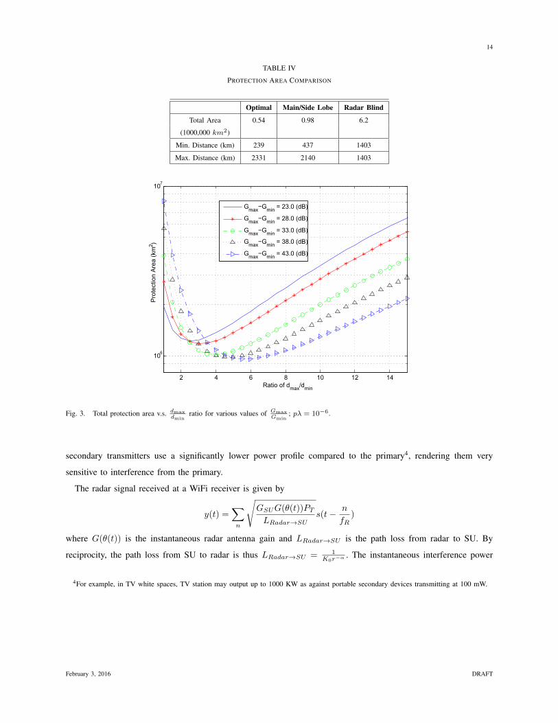
The best ratio β is selected to minimize total protection area of Area = [β2θH/2+π−θH/2]d2min. For pλ = 10−6

(time-space density product), figure 3 shows total protection area as a function of β for various values of Gmax

Gmin

(radio of maximum to minimum radar antenna gain).

Figure 4 shows protection distance as a function of relative azimuth with radar’s main beam for three cases

of Radar-Blind SU, Optimal Distance and Main/Side lobe interferer. It is evident from this figure that a radar-

blind SU will lose a significant portion of available white space spectrum as protection distance is significantly

larger than other two cases. Main/Side interferer is plotted for the optimum choice of β. It provides a much closer

distance to optimal results. A comparison between optimal distances here with that of single user in Figure 1 reveals

that distances are significantly increased (10-km for side lobes is expanded to 239-km) because of accumulated

interference from spatial distribution of users. Table IV compares total protection area for the three cases above.

While total area occupied by main/side lobe interferer is about twice the optimal area, the required area for radar-

blind user is 11.5 times larger than optimal, which again highlights the price to be paid for lack of information.

V. INTERFERENCE TO WIFI DEVICES

The main goal of spectrum sharing is to create new secondary networks, while providing protection to the

incumbents (primary). Therefore, it is essential to study primary to secondary interference. In most sharing scenarios,


14

TABLE IV

PROTECTION AREA COMPARISON

Optimal Main/Side Lobe Radar Blind

Total Area 0.54 0.98 6.2

(1000,000 km2)

Min. Distance (km) 239 437 1403

Max. Distance (km) 2331 2140 1403

2 4 6 8 10 12 14

106

107

RatioBofBdmax

/dmin

Pro

tect

ionB

Are

aB(k

m2 )

Gmax−G

min=B23.0B(dB)

Gmax−G

min=B28.0B(dB)

Gmax−G

min=B33.0B(dB)

Gmax−G

min=B38.0B(dB)

Gmax−G

min=B43.0B(dB)

Fig. 3. Total protection area v.s. dmaxdmin

ratio for various values of GmaxGmin

; pλ = 10−6.

secondary transmitters use a significantly lower power profile compared to the primary4, rendering them very

sensitive to interference from the primary.

The radar signal received at a WiFi receiver is given by

y(t) =∑n

√GSUG(θ(t))PTLRadar→SU

s(t− n

fR)

where G(θ(t)) is the instantaneous radar antenna gain and LRadar→SU is the path loss from radar to SU. By

reciprocity, the path loss from SU to radar is thus LRadar→SU = 1K0r−α

. The instantaneous interference power

4For example, in TV white spaces, TV station may output up to 1000 KW as against portable secondary devices transmitting at 100 mW.


15

−150 −100 −50 0 50 100 1500

500

1000

1500

2000

2500

RelativesAzimuthsw.r.t.sRadarsMainsBeamsbdegreeI

Pro

tect

ions

Dis

tanc

esbk

mI

OptimalsDistance

RadarsBlindsUser

Main/SidesLobesInterferer

Fig. 4. Protection region v.s. relative azimuth between SU and radar’s main antenna beam for following cases: Radar-Blind SU, Optimal

Protection Distance and Main/Side lobe interferer; pλ = 10−6, Pout,max = 0.1

t

Am

plitud

e (d

B)

Pulse Width

Pulse Repetition Interval

20

-5

One Full Rotation

Fig. 5. Radar signals received at WiFi receiver behave as a non-stationary source of interference.

from the radar and resulting SINR at the input to the WiFi receiver can be written as

PR(t) = PTGSUG(θ(t))K0d−αRadar−SU

∑n

Π(t

PW− n

fR)

SINRSU (t) =PSUGSU

LSU−SU (N0BW + PR(t))(35)

The radar interference to WiFi receivers is non-stationary for two reasons. First, due to radar rotation, the

interference power varies periodically as a characteristic for search radars. Depending on rotation speed, this period

is typically of the order of seconds. Second, the transmitted signals by radar s(t−n/fR) consists of short pulses as

shown in Figure 5. For our typical aeronautical radar, the pulse width is 1µs and pulse repetition internal is about

1ms. Therefore, even when the radar main beam is directly aligned with WiFi receiver (G(θ(t)) is maximum),

there are inter-pulse durations with zero interference.


16

Analytical evaluation of WiFi performance against a non-stationary interferer such as a pulsed radar is substantially

more complicated than stationary ones for several reasons. First, depending on WiFi packet size and radar pulse

repetition interval, the impact of radar signal on WiFi packet reception can vary greatly. For example, packet lengths

in 802.11n can be vary from few hundreds of microseconds to several tens of milliseconds. Therefore, for pulse

repetition interval of 1ms, short packets can fall in between inter-pulse intervals with significant probability, while

longer packets almost surely overlap with radar pulses. Second, WiFi packets are composed of multiple OFDM

symbols each of duration 4µs [30]. A radar pulse of 1-µs width will collide with one symbol (or few symbols

when packet is very long) out of many in the packet. Depending on the channel code (convolutional or LDPC) and

selected MCS as well as the SNR of the interference-free channel, packet might still be decodeable. In addition,

certain OFDM symbols are more crucial than the others. A collision between PLCP header and radar pulses will

leave the entire packet undecodeable while impacted data symbols may be recovered by interleaving and channel

coding. Third, all practical implementations of WiFi MAC/PHY layers include rate adaptation mechanisms to choose

the best MCS based on channel condition. These algorithms are typically designed to converge to a steady state

response in presence of stationary noise and interference. A non-stationary interferer can degrade the performance

drastically unless smarter adaptation methods are designed which are aware of coexistence scenario.

A comprehensive WiFi performance study that considers all the aforementioned concerns is beyond the scope of

this paper. Here, our focus is the achievable throughput in WiFi given the sharing scenario. Therefore, we assume

that rate adaptation mechanism in WiFi always selects the best MCS for the current SINR. We consider a pair of

802.11n-based SUs in a 20-MHz channel with one spatial stream (1x1 SISO). The standard modulation and coding

schemes in 802.11n as well as achievable rates are shown in Table V. The minimum required SNR for each MCS,

corresponding to a 10% packet loss, is also provided. The SNR values are obtained from [31] which are based on

experimental measurements on an Intel Wireless Wi-Fi Link 5300 a/g/n.

TABLE V

STANDARD MODULATION AND CODING SCHEMES AND ACHIEVABLE DATA RATES FOR 802.11N SPECIFICATIONS. MINIMUM REQUIRED

SNR FOR EACH MCS, CORRESPONDING TO 10% PACKET LOSS, IS ALSO PROVIDED.

MCS Modulation Coding Rate Data Rate(Mbps) SNR

0 BPSK 1/2 6.5 4.5

1 QPSK 1/2 13.0 6.5

2 QPSK 3/4 19.5 8.0

3 16-QAM 1/2 26.0 10.5

4 16-QAM 3/4 39.0 13.5

5 64-QAM 2/3 52.0 17.5

6 64-QAM 3/4 58.5 19.5

7 64-QAM 5/6 65.0 21.5

The achievable throughput RSU (t) is a function of two factors; the instant SINR as in (35) that determines date

rate through Table V and the fraction of time SU is allowed to transmit, ρ(d). From previous analysis for a single


17

user or multiple users, there is a minimum separate distance d(θ(t)) that depends on the direction of radar’s main

beam. ρ(d) defines the fraction of time when dRadar−SU ≥ d(θ(t)). Therefore, SU throughput is:

RSU (t) =

f(SINR(t)) dRadar−SU ≥ d(θ(t))

0 dRadar−SU < d(θ(t))(36)

Therefore, a closer SU to radar has a lower throughput not only due to reduced SINR but also diminished

transmission opportunity. The ρ(d) factor also depends on our sharing policy. For example, for a Radar-Blind

SU, ρ(d) is a binary function while for Main/Side lobe interferer, it is constant as long as d < dmax.

−150 −100 −50 0 50 100 1500

10

20

30

40

50

60

70

RadarUAzimuthU(Degree)

Thr

ough

putU(

Mbp

s)

UserU1,UDistanceU=U15Ukm



Fig. 6. Secondary user throughput for single-SU sharing with radar.

Figure 6 shows achievable throughput by SU for a single user sharing scenario with radar. Three different users are

considered at different distances from the radar and throughput variation is depicted with respect to radar rotation.

The path loss between WiFi AP and station is set to 80 dB, corresponding to free space loss for a 100-meter link

at 2.7GHz. As a first order approximation, SINR is set to instantaneous SINR as defined by (35), treating radar

pulses as a continuous waveform (CW) interfering with WiFi OFDM symbols.

In order to differentiate radar pulses from a CW signal, we need to estimate effective SINR from (35). Since

WiFi data are interleaved in time, an OFDM symbol (4-µs long) that falls within a radar pulse is later extended

to (after de-interleaving) a significantly larger time interval. This is equivalent to extending radar pulse width

while reducing its power level. Therefore, if we assume that WiFi interleaver is sufficiently long, effective radar

interference is PR(t) = PWfRPTGSUG(θ(t))K0d−αRadar−SU , which is averaged over pulse repetition interval. Here,

radar interference to WiFi receiver is scaled by a factor of pulse width/pulse repetition interval. The average SINR


18

101

102

103

0

10

20

30

40

50

60

70

DistancebtobRadarbLkmI

Thr

ough

putbL

Mbp

sI

SinglebUserbSharing

MultiplebSUbwithbOptimumbDistanceMultiplebSU,bMain/SidebLobebInterferer

MultiplebSU,bBlindbDistance

Fig. 7. Average secondary user throughput for single/multiple SU sharing with radar.

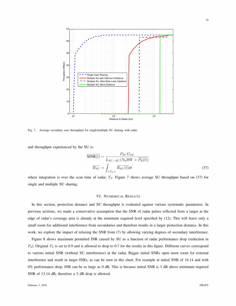
and throughput experienced by the SU is:

SINR(t) =PSUGSU

LSU−SU (N0BW + PR(t))

RSU =

∫<TS>

RSU (t)dt (37)

where integration is over the scan time of radar, TS . Figure 7 shows average SU throughput based on (37) for

single and multiple SU sharing.

VI. NUMERICAL RESULTS

In this section, protection distance and SU throughput is evaluated against various systematic parameters. In

previous sections, we made a conservative assumption that the SNR of radar pulses reflected from a target at the

edge of radar’s coverage area is already at the minimum required level specified by (12). This will leave only a

small room for additional interference from secondaries and therefore results in a larger protection distance. In this

work, we explore the impact of relaxing the SNR from (7) by allowing varying degrees of secondary interference.

Figure 8 shows maximum permitted INR caused by SU as a function of radar performance drop (reduction in

Pd). Original Pd is set to 0.9 and is allowed to drop to 0.7 for the results in this figure. Different curves correspond

to various initial SNR (without SU interference) at the radar. Bigger initial SNRs open more room for external

interference and result in larger INRs, as can be seen in this chart. For example at initial SNR of 16.14 and with

0% performance drop, INR can be as large as 0 dB. This is because initial SNR is 3 dB above minimum required

SNR of 13.14 dB, therefore a 3 dB drop is allowed.


19

0 2 4 6 8 10 12 14 16 18 20−20

−15

−10

−5

0

5

Radar.Performance.Drop.(%)

INR

.(dB

)

Interference.free.SNR.=.13.14.dB


Interference.free.SNR.=.15.14.dBInterference.free.SNR.=.16.14.dB


Fig. 8. Maximum permitted INR versus radar performance drop for various values of original SNR (interference-free SNR)

Using parameters in Table VI, the initial SNR at the radar input is estimated to be 30.57 dB which allows

maximum INR of +17.69 dB for 5% drop in Pd. We use this INR in the following to determine a less conservative

protection distance then previous sections as well as achievable SU throughput.

A. Protection Distance

Figure 9 shows protection distances for single and multiple SU sharing. Comparing this with Figs. 1 and 4 reveals

that protection distances are immensely reduced because INR is increased from -10.96 dB to +17.69 dB. To better

investigate the effect of initial radar SNR on required protection distances, Fig. 10 shows protection distance for

single/multiple radar-blind secondary users with different initial radar SNR. The minimum required SNR for target

ROC point of Pd=0.90 and Pfa = 10−6 is 13.4 dB. Therefore, for the initial SNR of 13.14 dB, the allowed radar

performance drop (because of additional interference) has significant impact on the protection distance. However,

if initial SNR is above this limit by only a few dB, the dependency of protection distance on radar performance

drop is significantly reduced. For example at SNR of 17.14 dB, increasing radar Pd drop from 90% to 70% will

reduce the distance from 315 km to 260 km (multiple SU, radar-blind).

In sharing radar spectrum with distributed SUs, the average interference is also highly affected by population

density and probability of WiFi network’s activity. Figure 11 shows this dependency by evaluating protection

distance for radar-blind users versus the product of pλ and for different initial radar SNR. A constant performance

drop of 5% is utilized for radar. It is clear from this figure that in the logarithmic scale, protection distance is a

linear function of pλ.


20

−f5I −fII −5I I 5I fII f5II

fI

2I

3I

4I

5I

6I

7I

8I

9I

RelativegAzimuthgwLrLtLgRadargMaingBeamgUdegree,

Pro

tect

iong

Dis

tanc

egUk

m,

MultigUser/gOptimal

MultigUser/gMainbSidegLobegInterfererMultigUser/gRadargBlindgUser

SinglegUser/gOptimal

Fig. 9. Protection distance versus azimuth for single and multi-user sharing

0 2 4 6 8 10 12 14 16 18 2030

35

40

45

50

55

60

Pro

tect

ionf

Dis

tanc

ef.k

mB,

fSin

glef

SU

0 2 4 6 8 10 12 14 16 18 20200

400

600

800

1000

1200

1400

RadarfPerformancefDropf.IB

Pro

tect

ionf

Dis

tanc

ef.k

mB,

fMul

tiple

fSU

InitialfSNRf=f13.14fdB


InitialfSNRf=f15.14fdBInitialfSNRf=f16.14fdB




InitialfSNRf=f15.14fdBInitialfSNRf=f16.14fdB


Fig. 10. Protection distance versus radar performance drop for single/multiple radar-blind secondary users. Initial SNR corresponds to noise-

limited SNR at radar receiver.


21

10−7

10−6

10−5

10−4

10−3

101

102

103

104

105

Time−SpatialdDensityd(pλ)

Pro

tect

iond

Dis

tanc

ed(k

m),

dRad

ar−

Blin

ddS

U

InitialdSNRd=d13.14ddB


InitialdSNRd=d15.14ddBInitialdSNRd=d16.14ddB


Fig. 11. Protection distance versus time-spatial density of WiFi networks, pλ

B. SU Throughput

By increasing initial radar SNR or allowing further drop in its performance, we observed significant reductions

in protection distances as shown in previous results. Reduced distances provide additional white space opportunities

for WiFi devices. On the other hand, closer distances to radar means additional interference from transmitted pulses.

The average interference from radar to WiFi receiver was calculated in (37) by scaling peak power with the ratio

of pulse width to pulse repetition interval. For our radar parameters, this translates to 1µs896µs ≈ 29.5 dB reduction

in effective radar interference level which significantly improves WiFi SINR at close distances to radar. Figure 12

shows achievable SU throughput for both cases of using peak radar interference (a) and average/effective radar

interference (b) to WiFi receivers (29.5 dB reduction w.r.t. peak). Initial radar SNR is set to 23.14-dB which is

10-dB above minimum required level and radar performance drop is set to 5%. For a radar-blind SU that can only

coexist with radar at large distances of >120 km, throughput is the same in both cases because radar interference is

negligible. However, at close distances of single-user sharing and multi-user with optimal distance, throughput drop

due to radar interference is very clear in (a). Particularly for the case of single-user sharing, protection distance is

reduced to about 2-km, but practical throughput is still zero up to 12 km from radar.

VII. CONCLUSION

In this paper, we considered the problem of spectrum sharing between a rotating radar and WiFi networks.

Minimum required SNR for noise-limited operation of the radar was defined as a function of basic radar parameters,

including probability of detection. Coexistence with WiFi users was made possible by permitting a certain drop in


22

0 20 40 60 80 100 120 140 160 180 2000

10

20

30

40

50

60

70

/aLMDistanceMtoMRadarM/kmL

Thr

ough

putM/

Mbp

sL

SingleMUserMSharing

MultipleMSUMwithMOptimumMDistance

MultipleMSUBMMain/SideMLobeMInterferer

MultipleMSUBMBlindMDistance

0 20 40 60 80 100 120 140 160 180 2000

10

20

30

40

50

60

70

/bLMDistanceMtoMRadarM/kmL

Thr

ough

putM/

Mbp

sL

SingleMUserMSharing

MultipleMSUMwithMOptimumMDistanceMultipleMSUBMMain/SideMLobeMInterferer

MultipleMSUBMBlindMDistance

Fig. 12. Achievable SU throughput versus distance for various sharing policies. (a) is based on peak radar interference to WiFi receiver and

(b) is based on average radar interference.

radar’s detection performance. We showed that this performance drop is very essential when radar SNR (without

interference from WiFi users) is very close to the minimum required SNR. This determined maximum tolerable

interference by the radar from WiFi devices (INR). Evaluating INR for various values of radar detection drops

revealed that INR falls abruptly at small performance detection drops, when radar SNR is already at its minimum;

otherwise INR changes are slow.

Protection distance - the minimum required distance between SU and radar receiver - was calculated for both

single-SU case as well as multiple spatially distributed SUs. The latter formed a Poisson point process in space

and an aggregate interference to radar that was approximated as Gaussian. Outage probability was utilized as the

defining metric for protection distance calculation and different sharing scenarios was introduced based on how

much radar-related data is available to the SU.

The optimal protection distance was defined in terms of minimizing total protected area. It was shown to be

proportional to G1α (θ). For a radar-blind SU, a constant protection distance was defined which was significantly

larger than optimal distance. Comparing total protected area for these two showed that radar-blind area is about 12

times (for our settings) larger than optimal area. A more pragmatic solution is an SU with sufficient side information

about radar to distinguish main lobe from side lobe. Protection distance for this type of SU was calculated and

shown to be very close to optimal distance.

The effect of interference caused by radar pulses on performance of WiFi networks was modeled and achievable

throughput (as a function of radar rotation as well as average) was estimated. For close distances to radar, throughput


23

was shown to be very low even though SU is allowed to transmit. Since radar interference is non-stationary, two

cases were considered as the upper and lower bounds of effective radar interference. First, instantaneous interference

from radar pulses was utilized for calculating effective SINR. Second, the power of radar pulses was normalized

by the ratio of pulse-width/pulse-repetition-interval. The former showed significant throughput reduction at close

distance (single SU and optimal multiple SU).

REFERENCES

[1] Global mobile data traffic forecast update, 2011-2016. From Cisco visual networking index. [Online]. Available: http:

//www.cisco.com/en/US/solutions/collateral/ns341/ns525/ns537/ns705/ns827/white paper c11520862.html

[2] In the Matter of Unlicensed Operation in the TV Broadcast Bands: Third Memorandum Opinion And Order, FCC Std. 12-36, April 2012.

[3] F. Hessar and S. Roy, “Capacity Considerations for Secondary Networks in TV White Space,” IEEE Trans. Mobile Comput., 2014 (to

appear).

[4] M. Tercero, K. Sung, and J. Zander, “Exploiting temporal secondary access opportunities in radar spectrum,” Wireless Personal

Communications, vol. 72, no. 3, pp. 1663–1674, 2013.

[5] Strategic Technology Office, “Shared spectrum access for radar and communications (ssparc),” Broad Agency Announcement, February

2013.

[6] R. Saruthirathanaworakun, J. Peha, and L. Correia, “Opportunistic sharing between rotating radar and cellular,” Selected Areas in

Communications, IEEE Journal on, vol. 30, no. 10, pp. 1900–1910, 2012.

[7] R. Saruthirathanaworakun, “Gray-space spectrum sharing with cellular systems and radars, and policy implications,” Ph.D. Thesis, Carnegie

Mellon University, 2012.

[8] R. Saruthirathanaworakun, J. Peha, and L. Correia, “Gray-space spectrum sharing between multiple rotating radars and cellular network

hotspots,” in Vehicular Technology Conference (VTC Spring), 2013 IEEE 77th, June 2013, pp. 1–5.

[9] F. Paisana, J. Miranda, N. Marchetti, and L. DaSilva, “Database-aided sensing for radar bands,” in Dynamic Spectrum Access Networks

(DYSPAN), 2014 IEEE International Symposium on, April 2014, pp. 1–6.

[10] M. Tercero, K. W. Sung, and J. Zander, “Impact of aggregate interference on meteorological radar from secondary users,” in Wireless

Communications and Networking Conference (WCNC), 2011 IEEE, March 2011, pp. 2167–2172.

[11] H. Shajaiah, A. Khawar, A. Abdel-Hadi, and T. Clancy, “Resource allocation with carrier aggregation in lte advanced cellular system

sharing spectrum with s-band radar,” in Dynamic Spectrum Access Networks (DYSPAN), 2014 IEEE International Symposium on, April

2014, pp. 34–37.

[12] M. Rahman and J. Karlsson, “Feasibility evaluations for secondary lte usage in 2.7-2.9ghz radar bands,” in Personal Indoor and Mobile

Radio Communications (PIMRC), 2011 IEEE 22nd International Symposium on, Sept 2011, pp. 525–530.

[13] H. Deng and B. Himed, “Interference mitigation processing for spectrum-sharing between radar and wireless communications systems,”

Aerospace and Electronic Systems, IEEE Transactions on, vol. 49, no. 3, pp. 1911–1919, July 2013.

[14] “Presentation: spectrum with significant federal commitments, 225 mhz - 3.7 ghz,” US National Telecommunications and Information

Administration (NTIA), 2009.

[15] 3.5 GHz Spectrum Access System Workshop and Online Discussion. [Online]. Available: http://www.fcc.gov/blog/

35-ghz-spectrum-access-system-workshop-and-online-discussion

[16] “Coexistence of S Band radar systems and adjacent future services,” Ofcom, Tech. Rep., December 2009.

[17] F. H. Sanders, J. E. Carroll, G. A. Sanders, and R. L. Sole, “Effects of Radar Interference on LTE Base Station Receiver Performance,” U.S.

Derpatment Of Commerce, National Telecommunications and Information Administration, Tech. Rep. NTIA Report 14-499, December

2013.

[18] ITU, “Characteristics of radiolocation radars, and characteristics and protection criteria for sharing studies for aeronautical radionavigation

and meteorological radars in the radiodetermination service operating in the frequency band 2700-2900 MHz,” International Telecommu-

nication Union, Tech. Rep., 2000-2003.

[19] “Characteristics of and protection criteria for sharing studies for radiolocation, aeronautical radionavigation and meteorological radars

operating in the frequency bands between 5250 and 5850 MHz,” ITU, Tech. Rep. Rec. ITU-R M.1638, 2003.


http://www.cisco.com/en/US/solutions/collateral/ns341/ns525/ns537/ ns705/ns827/white_paper_c11520862.html

http://www.cisco.com/en/US/solutions/collateral/ns341/ns525/ns537/ ns705/ns827/white_paper_c11520862.html

http://www.fcc.gov/blog/35-ghz-spectrum-access-system-workshop-and-online-discussion

http://www.fcc.gov/blog/35-ghz-spectrum-access-system-workshop-and-online-discussion

24

[20] F. H. Sanders, R. L. Sole, J. E. Carroll, G. S. Secrest, and T. L. Allmon, “Analysis and Resolution of RF Interference to Radars Operating in

the Band 2700-2900 MHz from Broadband Communication Transmitters,” U.S. Department Of Commerce, National Telecommunications

and Information Administration, Tech. Rep., October 2012.

[21] E. F. Drocella, L. Brunson, and C. T. Glass, “Description of a model to compute the aggregate interference from radio local area networks

employing dynamic frequency selection to radars operating in the 5 ghz frequency range,” National Telecommunications and Information

Administration (NTIA), Tech. Rep., May 2009.

[22] H. Griffiths, L. Cohen, S. Watts, E. Mokole, C. Baker, M. Wicks, and S. Blunt, “Radar spectrum engineering and management: Technical

and regulatory issues,” Proceedings of the IEEE, vol. 103, no. 1, pp. 85–102, Jan 2015.

[23] Frank H. Sanders, Robert L. Sole, Brent L. Bedford, David Franc, Timothy Pawlowitz, “Effects of RF Interference on Radar Receivers,” U.S.

Department of Commerce, National Telecommunications and Information Administration, Tech. Rep. NTIA Report TR-06-444, September

2006.

[24] Nadav Levanon, Radar Principles, 1st ed. United States of America: John Wiley and Sons, 1988.

[25] W. Alberhseim, “A closed-form approximation to robertson’s detection characteristics,” Proceedings of the IEEE, vol. 69, no. 7, pp.

839–839, July 1981.

[26] H. Ochiai and H. Imai, “On the distribution of the peak-to-average power ratio in ofdm signals,” Communications, IEEE Transactions on,

vol. 49, no. 2, pp. 282–289, Feb 2001.

[27] G. A. Hufford, “The ITS Irregular Terrain Model,” Institute for Telecommunication Services, Tech. Rep., September 1984, version 1.2.2,

The Algorithm Available on http://www.its.bldrdoc.gov/resources/radio-propagation-software/itm/itm.aspx.

[28] M. Haenggi and R. K. Ganti, “Interference in large wireless networks,” Found. Trends Netw., vol. 3, no. 2, pp. 127–248, Feb. 2009.

[Online]. Available: http://dx.doi.org/10.1561/1300000015

[29] K. W. Sung, M. Tercero, and J. Zander, “Aggregate interference in secondary access with interference protection,” Communications Letters,

IEEE, vol. 15, no. 6, pp. 629–631, June 2011.

[30] R. Van Nee, V. Jones, G. Awater, A. Van Zelst, J. Gardner, and G. Steele, “The 802.11n MIMO-OFDM Standard for Wireless LAN and

Beyond,” Wireless Personal Communications, vol. 37, no. 3-4, pp. 445–453, 2006.

[31] D. C. Halperin, “Simplifying the Configuration of 802.11 Wireless Networks with Effective SNR,” Ph.D. Thesis, University of Washington,

2012.

[32] D. Evans and M. D. Gallagher, “Potential Interference From Broadband Over Power Line (BPL) Systems To Federal Government

Radiocommunications At 1.7 - 80 MHz,” U.S. Department of Commerce, National Telecommunications and Information Administration,

Tech. Rep. NTIA Report 04-413, April 2004, Section 4: Characterization Of Federal Government Radio Systems And Spectrum Usage.

APPENDIX

A. Radar Parameters

Radar parameters used for simulation purposes in this paper are presented in table VI.

B. Optimum Protection Distance

Based on equations (29) and (30), optimal protection distance by limiting maximum outage probability is obtained

as:

dopt = arg mind(θ)

∫ 2π

0

d2(θ)

2dθ

µI + σIQ−1 (Pout,max) ≤ Imax

2P0N: No modulating signal and no information transmitted [32]3Options are: continuous, random, 360 deg, sector, etc.


http://dx.doi.org/10.1561/1300000015

25

TABLE VI

TECHNICAL PARAMETER FOR TYPE B AERONAUTICAL RADAR

Characteristics Radar B

Platform Type Ground, ATC

Tuning Range (MHz) 2700 - 2900

Modulation P0N5

Tx power into antenna 1.32 MW

Pulse Width (µs) 1.03

Pulse rise/fall time (µs) –

Pulse repetition rate (pps) 1059 - 1172

Duty Cycle 0.14 maximum

Chirp BW NA

Compression Ratio NA

RF emission BW (-20 dB) 5 MHz

RF emission BW (3 dB) 600 kHz

Antenna Parameters

Type Parabolic reflector

Pattern type (degrees) Cosecant-squared +30

Polarization Vertical or right hand circular

Main beam gain (dBi) 33.5

Elevation beamwidth (degree) 4.8

Azimuthal beamwidth (degree) 1.3

Horizontal scan rate (degree/s) 75

Horizontal scan type6(degrees) 360

Vertical scan rate (degree/s) N/A

Vertical scan type (degree) N/A

Side-lobe levels (1st and remote) 7.3dBi

Height (m) 8.0

Receiver Parameters

IF 3 dB bandwidth 653 kHz

Noise figure (dB) 4.0 maximum

Minimum discernible signal (dBm) -108

Receiver RF 3 dB bandwidth (MHz) 10

where µI and σI are calculated in (25) and (26):

µI = CµI

∫θ

G(θ)d2−α(θ)dθ

σI =

√Cσ2

I

∫θ

G2(θ)d2−2α(θ)dθ

Optimal d(θ) is attained by converting the inequality constraint to equality. This follows because for any d(θ) for

which the strict inequality constraint holds, we can scale down d(θ) accordingly to increase µI , σI and achieve

equality constraint (note that 2− α < 0 and 2− 2α < 0). This will clearly result in a smaller objective function.

With equality constraint, we use Lagrange multiplier method with a dummy variable ε to redefine objective


26

function as

dopt = arg mind(θ)

∫ 2π

0

d2(θ)

2dθ + ε

(µI + σIQ

−1 (Pout,max)− Imax

)Taking partial derivatives of the new objective function with respect to d(θ) results in:

∂f

∂d(θ)= 0

d(θ) + ε

[∂µI∂d(θ)

+Q−1(Pout,max)∂σI∂d(θ)

]= 0

Replacing µI and σI :

d(θ) + ε

(2− α)CµIG(θ)d1−α(θ) +Q−1(Pout,max)Cσ2

I(2− 2α)G2(θ)d1−2α(θ)

2√Cσ2

I

∫θG2(θ)d2−2α(θ)dθ

= 0

Let X = G(θ)d−α(θ), the above equation can be written as 1 + ε[ΓX + ΛX2

]= 0, where Λ and Γ are

constant. Solving for X results in G(θ)d−α(θ) = −εΓ±√ε2Γ2−4εΛ

2εΛ . Therefore, d(θ) is proportional to G1α (θ).

The proportionality constant is found from the constraint equation:

d(θ) = γG(θ)1α

CµI

∫θ

G(θ)γ2−αG2−αα (θ)dθ +Q−1 (Pout,max)

√Cσ2

I

∫θ

G2(θ)γ2−2αG2−2αα (θ)dθ = Imax

which is simplified to:

γ2−αCµI

∫θ

G2α (θ)dθ + γ1−αQ−1 (Pout,max)

√Cσ2

I

∫θ

G2α (θ)dθ = Imax


Documents

Spectrum Sharing Between A Surveillance Radar … Sharing Between A Surveillance Radar and Secondary Wi-Fi Networks ... Abstract Co-existence between ... and 3100-3650 MHz for military