Spectral resolution: Hyperspectral Imagery - Gipsa-labjocelyn.chanussot/teaching/sicom_3... · Antonio J. Plaza University of Extremadura Cáceres, Spain E-mail: [email protected] Spectral

Antonio J. PlazaAntonio J. PlazaUniversity of Extremadura University of Extremadura

CCááceres, Spainceres, Spain

EE--mail: [email protected] mail: [email protected]

http://www.umbc.edu/rssipl/people/aplazahttp://www.umbc.edu/rssipl/people/aplaza

Spectral resolution:

Hyperspectral Imagery

Spectral resolution:

Hyperspectral Imagery

8-12 September 2008GIPSA-lab Grenoble, France

ContentsContents

1. Introduction to hyperspectral imaging

2. Specific challenges of hyperspectral data processing

3. Classification techniques for hyperspectral data analysis

4. Spectral unmixing techniques for hyperspectral data analysis

5. Lossy hyperspectral data compression

6. High performance computing in hyperspectral imaging

7. Algorithm demonstrations and practice

8. Summary and remarks









Spectral resolution: hyperspectral imagery

International Summer School on Very High Resolution Remote Sensing – September 8-12, 2008, Grenoble, France 1.1

Algorithms +

Efficient implementations

Introduction to hyperspectral imaging: course outline


Spectral mixture analysis: Determines the

abundance of materials (e.g. precision agriculture).

Characterization: Determines variability of

identified material (e.g. wet/dry sand, soil particle

size effects).

Identification: Determines the unique identity of

the foregoing generic categories (e.g. land-cover or

mineral mapping).

Discrimination: Determines generic categories of

the foregoing classes.

Classification: Separates materials into spectrally

similar groups (e.g., urban data classification).

Detection: Determines the presence of materials,

objects, activities, or events.

Spectral mixture analysis: Determines the

abundance of materials (e.g. precision agriculture).

Characterization: Determines variability of

identified material (e.g. wet/dry sand, soil particle

size effects).

Identification: Determines the unique identity of

the foregoing generic categories (e.g. land-cover or

mineral mapping).

Discrimination: Determines generic categories of

the foregoing classes.

Classification: Separates materials into spectrally

similar groups (e.g., urban data classification).

Detection: Determines the presence of materials,

objects, activities, or events.PanchromaticPanchromatic

Hyperspectral

(100’s of bands)

Hyperspectral

(100’s of bands)

Multispectral

(10’s of bands)

MultispectralMultispectral

(10’s of bands)

Levels of Spectral Information in Remote Sensing

Ultraspectral

(1000’s of bands)

Ultraspectral

(1000’s of bands)

Introduction to hyperspectral imaging: increased spectral resolution


Concept of hyperspectral imaging using NASA Jet Propulsion Laboratory’s Airborne Visible Infra-Red Imaging Spectrometer



AVIRIS (NASA/JPL) Hyperspectral Cubehttp://aviris.jpl.nasa.gov/html/aviris.freedata.html



Hyperspectral data used for demonstration:



Data set provided by Robert O. Green at NASA/JPL

AVIRIS data over lower Manhattan (09/15/01)

Reference information available from U.S. Geological Survey

Spatial location of thermal hot spots in WTC area

Introduction to hyperspectral imaging: preliminary demo

Demo: concept of hyperspectral imagingDemo: concept of hyperspectral imaging

Demo will be performed using ITTVIS Envi 4.5 (http://www.ittvis.com)


Military target detection

Mine detection

Crop stress location

Rare mineral detection

Infected trees location

Search-and-rescue

operations

DEFENSE & INTELLIGENCE

PRECISION AGRICULTURE

GEOLOGY

FORESTRY

PUBLIC SAFETY

• Many military and civilian applications require detection of targets or anomalies.

• Different background models result in different detectors.

• Hyperspectral imaging allows detection of full-pixel and subpixel targets.

Applications

Introduction to hyperspectral imaging: anomaly detection

Application example: anomaly detection


Introduction to hyperspectral imaging: demo on anomaly detection

Demo: anomaly detectionDemo: anomaly detection



ContentsContents



















Challenges in hyperspectral image processing

• The special characteristics of hyperspectral data pose several processing problems:

1. The high-dimensional nature of hyperspectral data introduces new types of

pixels, such as mixed pixels and subpixel targets. Also, the limited

availability of training samples impacts supervised classifiers.

2. There is a need to integrate the spatial and spectral information to take

advantage of the complementarities that both sources of information can

provide, in particular, for unsupervised data processing.

3. There is a need to develop parallel algorithm implementations, able to

speed up algorithm performance and to satisfy the extremely high

computational requirements of time-critical remote sensing applications.

• In this course, we have taken a necessary first step towards the understanding and

assimilation of the above aspects in the design of last-generation hyperspectral image

processing algorithms.

Challenges of hyperspectral data processing: summary


Presence of mixed pixels in hyperspectral data

Pure pixel

(water)

Mixed pixel

(soil + rocks)

Mixed pixel

(vegetation + soil)

0

1000

2000

3000

4000

5000

300 600 900 1200 1500 1800 2100 2400

Reflectance

0

1000

2000

3000

4000

300 600 900 1200 1500 1800 2100 2400

Wavelength (nm)

Reflectance

0

1000

2000

3000

4000

300 600 900 1200 1500 1800 2100 2400

Wavelength (nm)

Reflectance

Wavelength (nm)

Some particularities of hyperspectral data are not to be found in other types of image data:

• Mixed pixels (due to insufficient spatial resolution and mixing effects in surfaces)

• Sub-pixel targets (very important and crucial in many hyperspectral applications)

Challenges of hyperspectral data processing: mixed pixels


Integragion of spatial and spectral information

• Much effort has been given to processing hyperspectral image data in spectral terms.

• Data analysis is carried out without incorporating information about spatial context.

• There is a need to incorporate the image representation of the data in the analysis.

• Most available approaches consider spatial and spectral information separately.

• Several approaches considered in this course to achieve the desired integration.

Pixel spatial coor-

dinates randomly

shuffled

Spectral processing Spectral processingSame output

results

Challenges of hyperspectral data processing: integration


Why high performance computing is crucial?

Wildland Fires in Spain/Portugal (August 2005)

Imaged by MERIS sensor, European Space Agency

Biomass Burning: Sub-pixel temperatures

and extent, smoke, combustion products…

Environmental Hazards: Contaminants

(direct and indirect), geological substrate…

Coastal and Inland Waters: Chemical and

biological standoff detection, oil spill

monitoring and tracking...

Ecology: Chlorophyll, leaf water, lignin,

cellulose, pigments, structure,

nonphotosynthetic constituents…

Commercial Applications: Mineral

exploration, agriculture and forest status…

Military Applications: Detection of land

mines, tracking of targets, decoys...

Others: Human infrastructure, Medical...

Biomass Burning: Sub-pixel temperatures

and extent, smoke, combustion products…

Environmental Hazards: Contaminants

(direct and indirect), geological substrate…

Coastal and Inland Waters: Chemical and

biological standoff detection, oil spill

monitoring and tracking...

Ecology: Chlorophyll, leaf water, lignin,

cellulose, pigments, structure,

nonphotosynthetic constituents…

Commercial Applications: Mineral

exploration, agriculture and forest status…

Military Applications: Detection of land

mines, tracking of targets, decoys...

Others: Human infrastructure, Medical...

Challenges of hyperspectral data processing: computing


Fire Temperatures

Debris CompositionAsbestos

AVIRIS spectra were

used to measure fire

temperature, asbestos

contamination, and

debris spread.

0

2

4

6

8

10

12

14

400 700 1000 1300 1600 1900 2200 2500

Wavelength (nm)

AVIRIS

Estimate

ResidualWTC Hot Spot Area A

Hottest Spectrum

Temperature Estimate=928K

6% of the area

September 11th World Trade Center

Challenges of hyperspectral data processing: computing


ContentsContents



















DAIS 7915 Image over Pavia, Italy

Courtesy: Prof. Paolo Gamba, University of Pavia

Water Trees Asphalt Parking lot Bitumen Brick roofs Meadows Bare soil Shadows

Classification techniques: data set used for demonstration


Ground truth classes

Hyperspectral data set used in experimentsHyperspectral data set used in experiments

0

1

2

3

4

5

0 1 2 3 4 5

k1

k2

k3

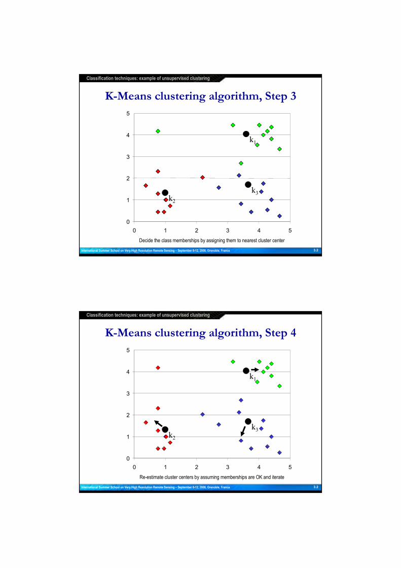
Classification techniques: example of unsupervised clustering

K-Means clustering algorithm, Step 1K-Means clustering algorithm, Step 1


Decide on a value for the initial cluster centers

0

1

2

3

4

5

0 1 2 3 4 5

k1

k2

k3



Initialize the cluster centers (randomly, if necessary)


0

1

2

3

4

5

0 1 2 3 4 5

k1

k2

k3



Decide the class memberships by assigning them to nearest cluster center


0

1

2

3

4

5

0 1 2 3 4 5

k1

k2

k3



Re-estimate cluster centers by assuming memberships are OK and iterate


Demo: unsupervised clusteringDemo: unsupervised clustering



Classification techniques: demo on unsupervised clustering

Spectral angle mapper (SAM)-based classification

x y

z

θθθθ

u = (x0, y0, z0)

v = (x1, y1, z1)

Only spetral distance able to deal with scaling introduced by illumination effects

Spectral angle distance:

Does not take into account

vector length (amount of

reflected radiation), only the

intrinsic characteristics of the

spectral signature (material

composition).

Classification techniques: spectral matching


Demo: spectral matchingDemo: spectral matching


Classification techniques: spectral matching


Demo: supervised classificationDemo: supervised classification


Classification techniques: supervised methods


• Nonlinear spatial-based technique that provides a framework to achieve the desired

integration of spatial and spectral data:

Binary erosion.-

K

Structuring

element

Classification techniques: morphological methods


• Nonlinear spatial-based technique that provides a framework to achieve the desired

integration of spatial and spectral data:

K

Structuring

element

Binary dilation.-



K

Structuring

element

Morphological opening (erosion + dilation)

• Opening and closing: shape-preserving operators.

• Excellent filtering properties:



Greyscale Mathematical Morphology

• Grayscale morphology relies on a partial ordering relation between image pixels.

Dilation

3x3 structuring element defines neighborhood around pixel P

Erosion

Max Min

P

Original image

Dilation

3x3 structuring element defines neighborhood around pixel P

Erosion

Max Min

P

Original image

• Morphological operations for hyperspectral imagery require ordering of image pixels.

• Two strategies explored in the past: PCA-based ordering and vector-based ordering.

(x,y)f

Grayscale image

Dilations

Structuring

B

element

Erosions



Morphological Profile.-

Uses opening and closing operations to create a feature vector for classification:

Extended Morphological Profile.-

Feature Extraction

PCA

PC1

PC2

PCn

Morphological

Profile

MP1

MP2

MPnExtended

MP

Provides information about the size of the structures (MP),

the local constrast (MP) and the spectrum (PCA).



Demo: morphological operations & filtersDemo: morphological operations & filters



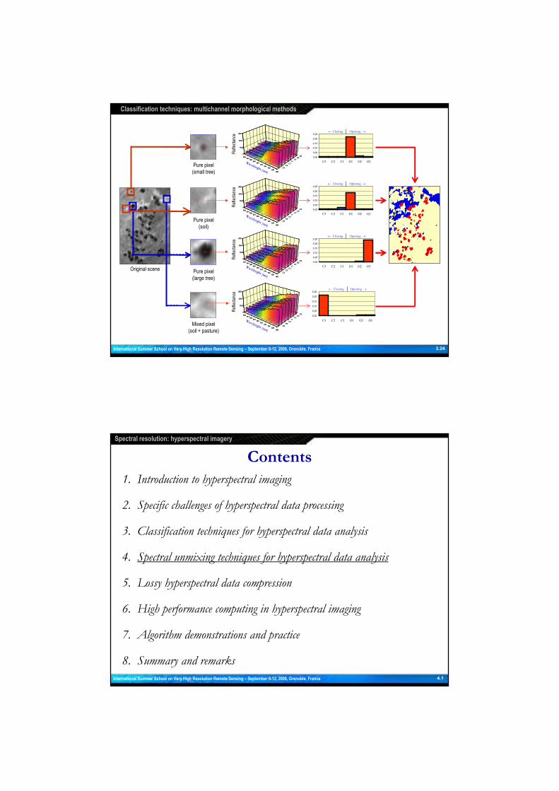
50% Vegetation + 50 % Soil

100% Vegetation pixels

100% Soil

N2ZZ: →f

Morphological profile using multichannel morphology.-

• Integration of spectral and spatial information (computation intensive)

• Selection of the most spectrally pure and the most spectrally mixed signatures.

( ) { }y)(x,(D arg_Min)y,x(K -

)K(Zt)(s, 2ff

∈

=⊗( ) { }y))(x,(D arg_Max)y,x(K

)K(Zt)(s, 2ff

+

∈

=⊕

Classification techniques: multichannel morphological methods


Original image

False color composition bands: 657, 551 and 496 nm

Multi-channel erosion

Disc SE radius=1 pixel (5 m)

Multi-channel dilation

Disc SE radius=1 pixel (5 m)



Processing examples:Processing examples:

DAIS/ROSIS data over Extremadura, Spain.-

• Obtained in of 2001 within HySens campaign of DLR at Extremadura, Spain.

• Dehesa semi-arid ecosystem formed by cork-oak trees, soil and pasture.

University of Extremadura

Guadiloba reservoir

Dehesa area



Original image

False color composition with

bands at 771, 619, and 543 nm


Disc SE radius=1 pixel (1.2 m)






Original image










Original image






Disc SE radius=1 pixel (1.2 m)Mixed pixel with soil and pasture




Original image







Mixed area surrounded by pure soil




Original image










Original image

Pure pixels have a derivative profile

unbalanced to the opening series

Multi-channel opening tends

to remove pure spatial areas




Original image

Mixed pixels have a derivative profile

unbalanced to the closing series

Multi-channel closing tends to

remove mixed spatial areas




0,00

0,05

0,10

0,15

0,20

0,25

C3 C2 C1 O1 O2 O3

Opening →← Closing

0,00

0,05

0,10

0,15

0,20

0,25

C3 C2 C1 O1 O2 O3


0,00

0,05

0,10

0,15

0,20

0,25

C3 C2 C1 O1 O2 O3



0,00

0,05

0,10

0,15

0,20

0,25

C3 C2 C1 O1 O2 O3

504544

584624

664704

744784

824

864

C3C2

C1P

O1

O2

O3

0

1000

2000

3000

504544

584624

664704

744784

824

864

C3C2

C1P

O1

O2

O3

0

1000

2000

3000

504544

584624

664704

744784

824

864

C3

C2C1

P

O1O2O3

0

1000

2000

3000

504544

584624

664704

744784

824864

C3

C2C1

P

O1O2O3

0

1000

2000

3000

Wavelenght (nm)

Reflectance

Wavelenght (nm)

Reflectance

Pure pixel (small cork-oak tree)

Wavelenght (nm)

Reflectance

Wavelenght (nm)

Reflectance

Pure pixel

(soil area)

Pure pixel

(large cork-oak tree)

Mixed pixel

(soil and pasture)

504544

584624

664704

744784

824

864

C3C2

C1P

O1

O2

O3

0

1000

2000

3000

504544

584624

664704

744784

824

864

C3C2

C1P

O1

O2

O3

0

1000

2000

3000

504544

584624

664704

744784

824

864

C3

C2C1

P

O1O2O3

0

1000

2000

3000

504544

584624

664704

744784

824864

C3

C2C1

P

O1O2O3

0

1000

2000

3000

Wavelenght (nm)

Reflectance

Wavelenght (nm)

Reflectance

Pure pixel (small cork-oak tree)

Wavelenght (nm)

Reflectance

Wavelenght (nm)

Reflectance

Pure pixel

(soil area)

Pure pixel

(large cork-oak tree)

Mixed pixel

(soil and pasture)

Original scene

Pure pixel

(small tree)

Pure pixel

(soil)

Pure pixel

(large tree)

Mixed pixel

(soil + pasture)

Reflectance

Reflectance

Reflectance

Reflectance



ContentsContents



















Soil

Tree

Grass

Macroscopic mixture:

15% soil, 25% tree, 60% grass in a 3x3 meter-pixel

12 meters1 2 meters

4 meters

4 meters

Intimate mixture:

Minerals intimately mixed in a 1-meter pixel

Increasing the spatial resolution of the sensor does not necessarily solve the problem!

• Mixed pixls can still be obtained at very high spatial resolutions (may complicate analysis)

• Intimate mixtures may take place regardless of the spatial resolution available

• Most available data compression strategies do not take into account such phenomena

• In this work, a simple spectral mixture analysis-based compression method is developed

by assuming that, in onboard data compression, spectral information may be more useful

than spatial information (which may be ultimately affected by posterior geometric corrections)

Presence of mixed pixels in hyperspectral data

Spectral unmixing techniques: presence of mixed pixels


Linear versus nonlinear mixing.-

• Linear mixture model

� Assumes that endmember substances are sitting side-by-side within the FOV.

• Nonlinear mixture model

� Assumes that endmember components are randomly distributed throughout the FOV.

� Multiple scattering effects.

Linear interaction

( ) )y,x(yx,)y,x( nMf +α= ( ) )y,x(yx,)y,x( nMf +α=

Nonlinear interaction

( )[ ] )y,x(yx, ,F)y,x( nMf +α= ( )[ ] )y,x(yx, ,F)y,x( nMf +α=

Mezcla lineal Mezcla no lineal

Spectral unmixing techniques: linear versus nonlinear unmixing


Linear interaction

( ) )y,x(yx,)y,x( nMf +α= ( ) )y,x(yx,)y,x( nMf +α=

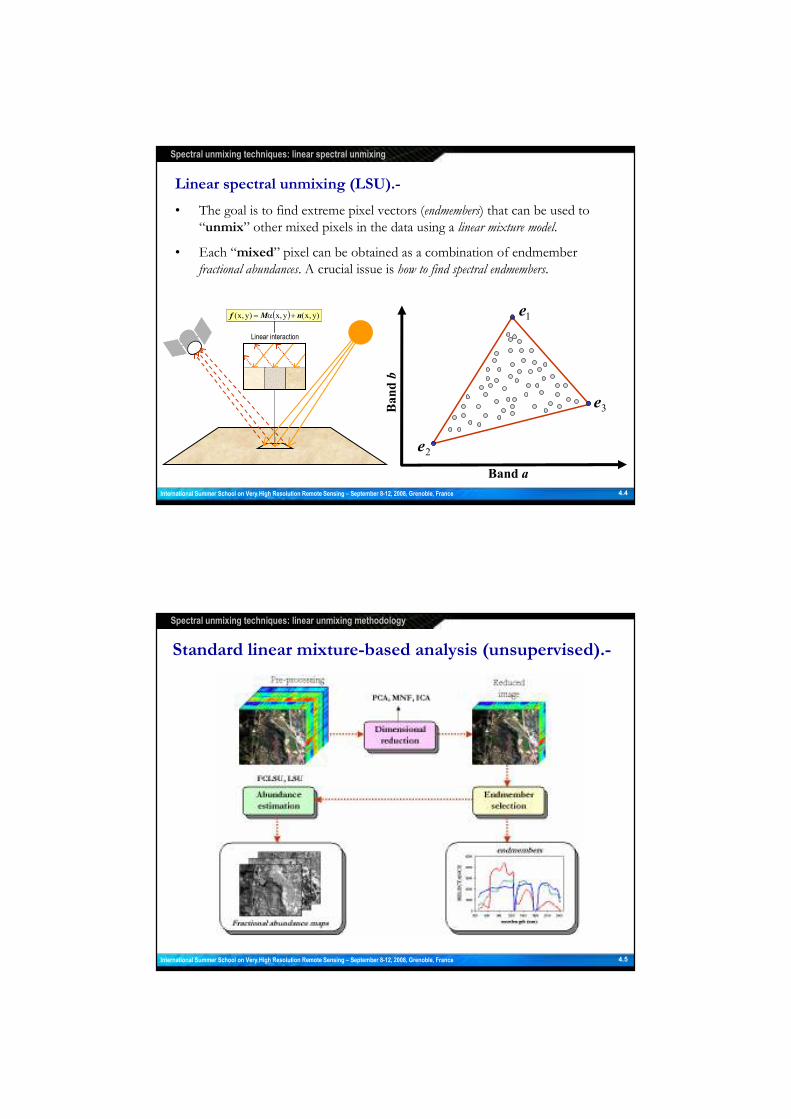
Linear spectral unmixing (LSU).-

• The goal is to find extreme pixel vectors (endmembers) that can be used to “unmix” other mixed pixels in the data using a linear mixture model.

• Each “mixed” pixel can be obtained as a combination of endmember fractional abundances. A crucial issue is how to find spectral endmembers.

Band a

Band b

1e

2e

3e

Spectral unmixing techniques: linear spectral unmixing


Standard linear mixture-based analysis (unsupervised).-

Spectral unmixing techniques: linear unmixing methodology


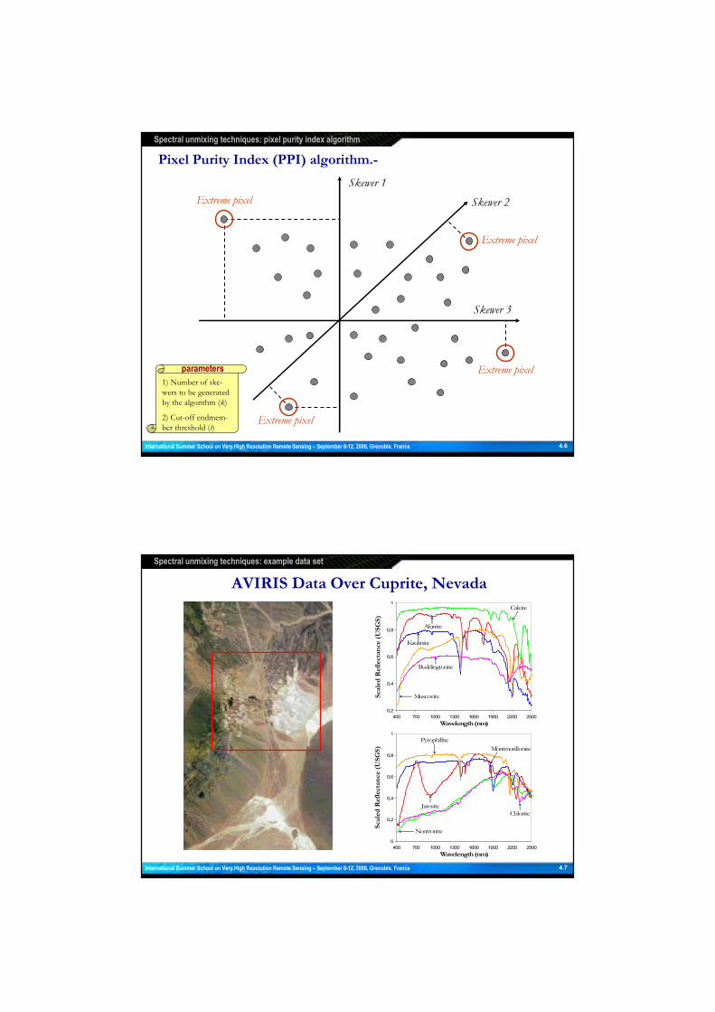
Extreme pixel

Extreme pixel

Extreme pixel

Extreme pixel

Skewer 1

Skewer 2

Skewer 3

Pixel Purity Index (PPI) algorithm.-

1) Number of ske-

wers to be generated

by the algorithm (k)

2) Cut-off endmem-

ber threshold (t)

parameters

Spectral unmixing techniques: pixel purity index algorithm


AVIRIS Data Over Cuprite, Nevada

0,2

0,4

0,6

0,8

1

400 700 1000 1300 1600 1900 2200 2500

Wavelength (nm)

Alunite

Calcite

Buddingtonite

Kaolinite

Muscovite

0

0,2

0,4

0,6

0,8

1

400 700 1000 1300 1600 1900 2200 2500

Wavelength (nm)

JarositeChlorite

Pyrophillite

Nontronite

Montmorillonite

Scaled Reflectance (USGS)

Scaled Reflectance (USGS)

Spectral unmixing techniques: example data set


Demo: endmember extractionDemo: endmember extraction




Demo: spectral unmixingDemo: spectral unmixing




Advanced Endmember Extraction (practice session).-

Skewer 1Skewer 1

Skewer 2Skewer 2

Skewer 3Skewer 3

Extreme pixel

Extreme pixel

Extreme pixel

Extreme pixel

Extreme pixelExtreme pixel


Pixel Purity Index (PPI)

Extreme pixel

Extreme pixel

Extreme pixel

Extreme pixel

Extreme pixel

Extreme pixel

Extreme pixel

Extreme pixel

N-FINDR algorithm

Spectral unmixing techniques: endmember extraction algorithms


Spatial/spectral competitive endmember extraction by morphological operations

Smin , Smax

Original

image

Automated

identification of

pure pixels

Endmember

abundance

estimation by FCLSU

MEI

image

end-members Adaptative

spatial/spectral

region growing

Redundant endmember

thinning

Automated Morphological Endmember Extraction (AMEE)

ContentsContents



















Standard hyperspectral analysis methodology

Lossy hyperspectral data compression: framework

Spectral unmixing

A simple, yet effective

strategy to compress a

hyperspectral data set

is to retain the spectral

endmembers (with high

spectral fidelity) and

the estimated (spatial)

abundance fractions


PPI/LSU hyperspectral data

compression algorithm

Instead of using the first step, we may

input the number of

endmembers as a

parameter to control

the compression ratio

remarks/comments

{ }Eii 1=

e

{ }Ei

aaa1E21 ,,,=

⋅⋅⋅=a

EE aaa ⋅+⋅⋅⋅+⋅+⋅= eeef 2211

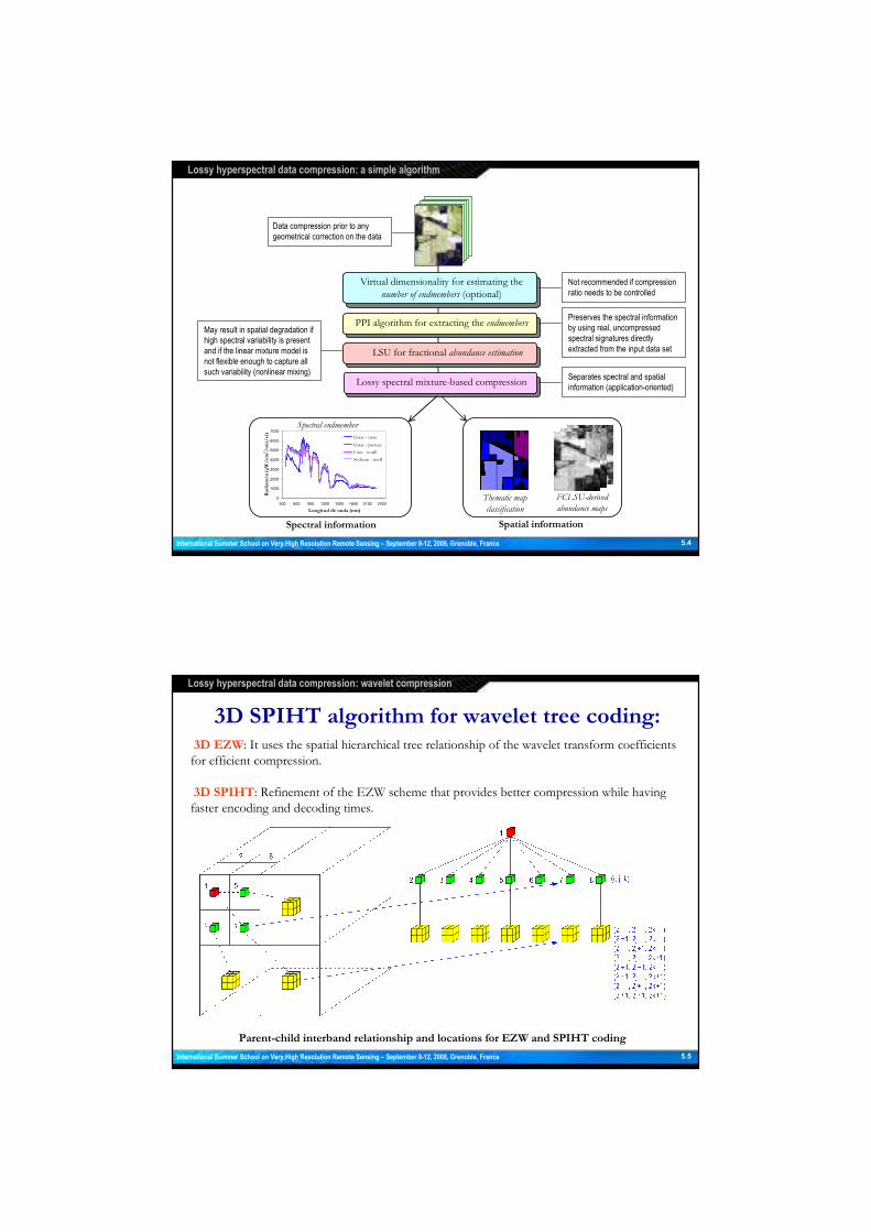
1. Estimate the number of spectral endmembers, E, in the input data

2. Use PPI algorithm to find a set of E image-derived endmembers

3. For each pixel vector f in the original image, use the LSU algorithm to estimate the corresponding endmember fractions:

4. Reconstruct each pixel vector as:

5. Construct E fractional abundance images, one for each endmember, and store them along with the spectral endmembers as a lossy representation of the original hyperspectral data cube

LSU-based hyperspectral compression algorithm

Lossy hyperspectral data compression: a simple algorithm


ImagenOriginal

Virtual dimensionality for estimating the number of endmembers (optional)

PPI algorithm for extracting the endmembers

FCLSU for fractional abundance estimation

Lossy spectral mixture-based compression

0

1000

2000

3000

4000

5000

6000

7000

300 600 900 1200 1500 1800 2100 2400

Longitud de onda (nm)

Radiancia (µW/cm

2/nm/sr)

Grass - trees

Grass - pasture

Corn - notill

Soybean - notill

Spectral information Spatial information

Spectral endmember

Thematic map

classification

FCLSU-derived

abundance maps

Not recommended if compression

ratio needs to be controlled

Preserves the spectral information

by using real, uncompressed

spectral signatures directly

extracted from the input data set

May result in spatial degradation if

high spectral variability is present

and if the linear mixture model is

not flexible enough to capture all

such variability (nonlinear mixing)Separates spectral and spatial

information (application-oriented)

Data compression prior to any

geometrical correction on the data

Lossy hyperspectral data compression: a simple algorithm


3D SPIHT algorithm for wavelet tree coding:

3D EZW: It uses the spatial hierarchical tree relationship of the wavelet transform coefficients

for efficient compression.

3D SPIHT: Refinement of the EZW scheme that provides better compression while having

faster encoding and decoding times.

Parent-child interband relationship and locations for EZW and SPIHT coding

Lossy hyperspectral data compression: wavelet compression


0

1000

2000

3000

4000

5000

6000

300 600 900 1200 1500 1800 2100 2400

Wavelength (nm)

Reflectance (%*100)

Soil Forest Chaparral ShadeGrass

Soil Forest Grass Chaparral Shade

ENVI 0.027 0.022 0.021 0.019 0.017

PPI 0.028 0.025 0.022 0.020 0.019

FPGA 0.028 0.025 0.022 0.020 0.019

N-FINDR 0.031 0.025 0.045 0.020 0.025

SMACC 0.043 0.041 0.032 0.031 0.025

AVIRIS scene over Jasper Ridge, CA (614x512x224)

PPI endmember extraction accuracy assessment:

Spectral angle scores between endmembers produced by ENVI’s PPI, a C-based PPI, and FPGA-PPI

Other standard endmember extraction algorithms (N-FINDR, IEA) are included in the comparison for validation purposes

Lossy hyperspectral data compression: effect of compression


Alunite Buddingt. Calcite Kaolinite Muscovite

ENVI 0.061 0.042 0.055 0.035 0.058

PPI 0.063 0.042 0.055 0.054 0.067

FPGA 0.063 0.042 0.055 0.054 0.067

N-FINDR 0.063 0.042 0.071 0.065 0.083

SMACC 0.063 0.042 0.055 0.054 0.078

AVIRIS scene over Cuprite, NV (614x512x224)

PPI endmember extraction accuracy assessment:

Spectral angle scores between endmembers produced by ENVI’s PPI, a C-based PPI, and FPGA-PPI

Other standard endmember extraction algorithms (N-FINDR, IEA) are included in the comparison for validation purposes

0,2

0,4

0,6

0,8

1

400 700 1000 1300 1600 1900 2200 2500

Wavelength (nm)

Alunite

Calcite

Buddingtonite

Kaolinite

Muscovite

Scaled reflectance

Lossy hyperspectral data compression: effect of compression


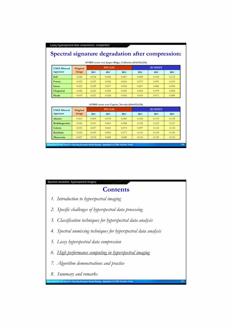
Spectral signature degradation after compression:

AVIRIS scene over Cuprite, Nevada (614x512x224)

0.1520.1390.1160.0890.0820.0740.067Muscovite

0.1460.1340.1100.0710.0620.0590.054Kaolinite

0.1340.1220.0970.0740.0630.0570.055Calcite

0.1270.1250.1020.0680.0610.0530.042Buddingtonite

0.1290.1190.1060.0850.0780.0690.063Alunite

80:140:120:180:140:120:1

3D SPIHTPPI/LSUOriginal

image

USGS Mineral

signature

0.0800.0720.0550.0420.0280.0210.019Shade

0.0840.0780.0620.0450.0290.0230.020Chaparral

0.0940.0860.0670.0540.0370.0290.022Grass

0.1030.0910.0730.0610.0420.0330.025Forest

0.1120.1020.0890.0670.0460.0340.028Soil

80:140:120:180:140:120:1

3D SPIHTPPI/LSUOriginal

image

USGS Mineral

signature

AVIRIS scene over Jasper Ridge, California (614x512x224)

Lossy hyperspectral data compression: comparison


ContentsContents



















• Parallel computer: a collection of processing elements that cooperate to solve problems faster

• Hyperspectral imaging demands parallel computers to speed-up many applications

• Speed-up (p processors) = Performance (p processors)

Performance (1 processor)

Earth Simulator (5120 processors)NASA Portable MiniCluster (16 processors)

Parallel computing using commodity clusters


High performance computing: challenges

Some problems to overcome:

– Radiation-hard design considerations

– Lack of standardized programming models

– Power consumption issues

– New technology

� Learning curve

� Integration with standard algorithms

� Fear of change by end-users

– Cost effectiveness of technology only demonstrated on selected projects

– Potential for high degree of project risk

– Need for proof of concept systems and simple algorithms

– Few techniques developed taking into account hyperspectral properties

– Most of them adapted from other problems (multimedia & video)

Many partners in hyperspectral imaging interested in onboard compression

Challenges of onboard data processing


High performance computing: challenges

Data partitioning strategies:

Spectral-domain partitioning:

A single pixel vector (spectral signature) may be

stored in different processing units and

communications would be required for individual

pixel-based calculations such as spectral angle

computations.

Spatial-domain partitioning:

Every pixel vector (spectral signature) is stored in

the same processing unit. This is beneficial for

the proposed sliding-window approach in terms

of low-level image processing and

spatial/spectral data integration.


High performance computing: hyperspectral data partitioning

1. The master divides the original image cube into a set of spatial-domain partitions:

4 processors 5 processors

Parallel implementation of PPI: “embarrasingly parallel”

max

max

max max1

max2

max3

2. The master generates a set of k random skewers and distributes the same set to all workers.

After projections, each worker sends local pixels selected more than t times to the master.

High performance computing: implementations on clusters


Thunderhead (NASA)http://thunderhead.gsfc.nasa.gov



1 4 16 36 64 100 144 196 256

P-PPI 1163 295 76 33 18 12 8 6 5

P-AMEE 916 261 60 34 18 12 9 7 6

P-FINDR 1263 366 97 39 21 14 9 7 6

P-OSP 948 218 70 35 18 13 10 8 7

Processing times (in seconds) for different numbers of processors (times of parallel application of LSU included)

P-PPI

P-AMEE

P-FINDR

P-OSP

IDEAL

http://thunderhead.gsfc.nasa.gov

Performance of parallel implementations on Thunderhead



Original imageClassification map

PSSP1 MEI1

Processing node #1

3x3 SE

MEI

PSSP2

Scatter

Processing node #2

3x3 SE

MEI

MEI2

Gather

Parallel Framework for Morphological Methods

• The master processor is in charge of distributing the work among the workers.

• Each partition (PSSP) is processed independently, and the master gathers the result.



Border-Handling Data Strategy Adopted in

Morphological Processing

Pixels which do not belong to the image domain are simply disregarded in the

calculation of the morphological eccentricity index (MEI)

PSSPj MEIj

3x3 SE

MEI



f(5,3)

Boundary

data

ifD

1i+fD

fD

Handling Communications (I)

Kernel-based computations prevent exploitation of the concept of PSSP since

communications are required for border pixels (simplified view).



Handling Communications (II)

Overlapping scatter

for 3x3 kernel

f(5,3)

ifD

1i+fD

fD

Overlapping scatter allows to process PSSPs independently through the

introduction of redundant information (several ways to do this!)



Performance of Morphological Endmember Extraction.-

• Algorithms were implemented in C++ using calls to Message Passing Interface (MPI).

• Using redundant computations versus communications was crucial:.

1 4 16 36 64 100 144 196 256

Redundant

comput.9452+13 4075+10 917+12 381+11 205+15 128+16 89+14 65+11 50+10

Interproc.

communic.3984+143 1128+151 889+160 371+194 205+225 124+243 83+261 62+268 49+292

Processing times (seconds) for different numbers of processors on Thunderhead (AVIRIS Cuprite)

0

32

64

96

128

160

192

224

256

0 32 64 96 128 160 192 224 256

Number of CPUs

Speedupp

1 iteration

3 iterations

5 iterations

Linear

0

32

64

96

128

160

192

224

256

0 32 64 96 128 160 192 224 256

Number of CPUs

Speedupp

1 iteration

3 iterations

5 iterations

Linear

Redundant computations Interprocessor communications



FPGA implementation of PPI/LSU:

• Xilinx Virtex-II FPGA with 33,792 slices, 144 Select RAM Blocks and 144 multipliers

(of 18-bit x 18-bit)

• One 3U Compact PCI card (weight below 1 lb) and power of approximately 25 Watts

• Complete system (systolic array plus PCI interface), implemented on XC2V6000-6

board, using different numbers of processors

PPI/LSU on Virtex-II FPGA with 33,792 slices, 144 RAM blocks and 144 multipliers

(moderate number of gates due to radiation-tolerance and certification considerations)


High performance computing: implementations on FPGAs

Extreme pixel

Extreme pixel

Extreme pixel

Extreme pixel





Skewer 1Skewer 1

Skewer 2Skewer 2

Skewer 3Skewer 3



Systolic array design for implementation of PPI:

�

�

dot11 dot12 dot13 dot1T



dotK1 dotK2 dotK3 dotKT

( ) ( )111 ,...,ff

� ( ) ( )∗

122 ,...,ff

� ( ) ( )∗∗

133 ,...,ff

� ( ) ( ){

1

1 ...,...,−

∗∗T

T�T ff

min1

min2

min3

minK

''∞

max1 max2 max3 maxT'0'

( ) ( )111 ,...,skewerskewer

�

( ) ( )∗

122 ,...,skewerskewer

�

( ) ( )∗∗

133 ,...,skewerskewer

�

( ) ( ){

1

1...,...,−

∗∗K

K�K skewerskewer



Implementation issues (PPI).-

• The figure depicts an ideal systolic array in

which T pixels and K skewers are processed.

• In a real systolic T has to be divided by

P, the number of available processors.

• A similar comment applies to K, the

number of skewers.

• After T/P cycles, all dot nodes are busy.

• After K/P additional cycles, the first P

pixel vectors are processed.

�

�




dotK1 dotK2 dotK3 dotKT

( ) ( )111 ,...,ff

� ( ) ( ) ∗122 ,...,ff

� ( ) ( ) ∗∗133 ,...,ff

� ( ) ( ){

1

1...,...,−

∗∗T

T�T ff( ) ( )1

11 ,...,ff� ( ) ( ) ∗1

22 ,...,ff� ( ) ( ) ∗∗1

33 ,...,ff� ( ) ( )

{1

1...,...,−

∗∗T

T�T ff

min1

min2

min3

minK

''∞

min1

min2

min3

minK

''∞

max1 max2 max3 maxT'0' max1 max2 max3 maxT'0'


�

( ) ( ) ∗122 ,...,skewerskewer

�

( ) ( ) ∗∗133 ,...,skewerskewer

�

( ) ( ){

1

1 ...,...,−

∗∗K

K�K skewerskewer


�

( ) ( ) ∗122 ,...,skewerskewer

�

( ) ( ) ∗∗133 ,...,skewerskewer

�

( ) ( ){

1

1 ...,...,−

∗∗K

K�K skewerskewer

Implementation issues (LSU).-

• To obtain the endmember abundances, we multiply each f by , where

• This can be done using the same systolic architecture used for the PPI algorithm

( ) T-1TMMM { }e

ii 1== eM



PPI algorithm rewritten:



Handel-C implementation of the PPI algorithm



Validation on real Xilinx Virtex-II platform:

Appealing perspectives from an exploitation point of view : on-the-fly selection

Number of processors

Number of gates

Number of slices

Percentage of total

Operation frequency

Processing time (secs)

100 97,443 1,185 3% 29,257 53.48

200 212,412 3,587 10% 21,782 22.65

400 526,944 12,418 36% 18,032 7.94

• An optimized C-based sequential implementation of PPI/LSU took 1163 seconds on

a desktop PC with AMD Athlon 2.6 GHz processor and 512 MB of RAM

• Our implementation was limited by the transfer rate: FPGA able to absorb a 40

Mbytes/second while PCI interface can only provide a flow of 15 Mbytes/second

• We decided to report realistic experiments by resorting to a moderate amount of

resources (gates) in the FPGA board (leaving room for implementation of additional

algorithms on the same board, allowing for on-the-fly algorithm selection)

• Results not strictly in real-time (below 5 seconds) but already very close



Doom3

nVidia Demo

Graphic processing units:

nVIDIA NV40 ATI R420

Reduced cost and decreasing:

GeForce 6800 Ultra Radeon X800 XT


Advent of commodity graphic processing units


Parallel implementation on Nvidia GPUs

PPI/LSU on Nvidia 7800 GTX

(Implementationin 8800 GTX available)


High performance computing: implementations on GPUs

• The advent of graphics processing units (GPUs) offers an unprecedented opportunity for

onboard hyperspectral data processing at low cost.

• GPUs can significantly accelerate the critical path of data parallel applications.

• GPUs now fully programmable using high-level languages such as CUDA

(http://developer.nvidia.com/object/cuda_get.html)

• More transistors devoted to data processing rather than data caching and control flow.

GPUs as the future of low-cost computing



http://www.nvidia.es/page/geforce_8800.htmlhttp://www.nvidia.es/page/geforce_8800.html




http://developer.nvidia.comhttp://developer.nvidia.com




ContentsContents



















SummarySummary• The special characteristics of hyperspectral images pose new processing problems, not

found in other types of remote sensing data.

• Kernel methods offer an interesting solution to deal with the high-dimensional nature

of the data and the limited availability of training samples (supervised classification).

• The integration of spatial and spectral information allows for the development of

enhanced supervised/unsupervised analysis techniques.

• Endmember extraction and spectral unmixing can greatly benefit from the use of

spatial information when designing techniques for estimating fractional abundances

and finding pure spectral signatures in the data.

• Most of the algorithms discussed in this course are very appealing for the design

of parallel implementations.

• Techniques presented in this course show the increasing sophistication of a field

that is rapidly maturing at the intersection of many different disciplines.

• The special characteristics of hyperspectral images pose new processing problems, not

found in other types of remote sensing data.

• Kernel methods offer an interesting solution to deal with the high-dimensional nature

of the data and the limited availability of training samples (supervised classification).

• The integration of spatial and spectral information allows for the development of

enhanced supervised/unsupervised analysis techniques.

• Endmember extraction and spectral unmixing can greatly benefit from the use of

spatial information when designing techniques for estimating fractional abundances

and finding pure spectral signatures in the data.

• Most of the algorithms discussed in this course are very appealing for the design

of parallel implementations.

• Techniques presented in this course show the increasing sophistication of a field

that is rapidly maturing at the intersection of many different disciplines.

Summary and remarks


Remarks on future directions Remarks on future directions • Soft classifiers are well suited to cope with the extremely high dimensionality of the

data, and also with the limited availability of training samples.

• We anticipate that the full adaptation of soft classifiers to mixed-pixel classification

problems (e.g., via multi-regression and robust training sample selection algorithms) may

push the frontiers of hyperspectral data classification to new application domains.

• Further developments on the joint exploitation of the spatial and the spectral

information in the input data are also needed.

• Advances in high performance computing environments including clusters of computers and

distributed grids, as well as specialized hardware modules such as field

programmable gate arrays (FPGAs) or graphics processing units (GPUs) will also be

crucial in many applications.

• We anticipate that the future potential of hyperspectral data classification methods

will be largely defined by their suitability for being efficiently implemented in parallel

(onboard implementations also highly desirable)

• Soft classifiers are well suited to cope with the extremely high dimensionality of the

data, and also with the limited availability of training samples.

• We anticipate that the full adaptation of soft classifiers to mixed-pixel classification

problems (e.g., via multi-regression and robust training sample selection algorithms) may

push the frontiers of hyperspectral data classification to new application domains.

• Further developments on the joint exploitation of the spatial and the spectral

information in the input data are also needed.

• Advances in high performance computing environments including clusters of computers and

distributed grids, as well as specialized hardware modules such as field

programmable gate arrays (FPGAs) or graphics processing units (GPUs) will also be

crucial in many applications.

• We anticipate that the future potential of hyperspectral data classification methods

will be largely defined by their suitability for being efficiently implemented in parallel

(onboard implementations also highly desirable)

Summary and remarks


A. Plaza, A. Mueller, R. Richter, T. Skauli, Z. Malenovsky, J. Bioucas, S. Hofer, J. Chanussot, C. Jutten, V. Carrere, I. Baarstad, P. Kaspersen, J. Nieke, K. Itten, T. Hyvarinen, P. Gamba, F. Dell’Acqua, J. A. Benediktsson, M. E. Schaepman,

J. Clevers and B. Zagajewski

HYPER-I-NET: European Research

Network on Hyperspectral Imaging

Consortium

Bogdan ZagajewskiWarsaw University (WURSEL), POLAND

Wageningen University (WUR), THE NETHERLANDS

Norsk Elektro-Optics (NEO), NORWAY

University of Iceland (UNIS), ICELAND

University of Pavia (UNIPV), ITALY

Spectral Imaging Oy, Ltd. (SPECIM), FINLAND

Remote Sensing Laboratories, University of Zurich (UZH), SWITZERLAND

Laboratory of Planetology and Geodynamics (CNRS), FRANCE

Technical Institute of Grenoble (INPG), FRANCE

Kayser-Threde Gmbh (KT), GERMANY

Instituto Superior Técnico (IST), PORTUGAL

Institute of Systems Biology and Ecology (ISBE), CZECH REPUBLIC

Norwegian Defence Research Establishment (FFI), NORWAY

German Remote Sensing Data Center (DLR), GERMANY

University of Extremadura (UEX), SPAIN

Participating institutions:

Michael Schaepman

Peter Kaspersen

Jon Atli Benediktsson

Paolo Gamba

Timo Hyvarinen

Klaus Itten, Jens Nieke

Veronique Carrere

Jocelyn Chanussot

Stefan Hofer

José Bioucas Dias

Zbynek Malenovsky

Torbjorn Skauli

Andreas Mueller

Antonio J. Plaza (coordinator)

Scientist in charge:

International School on Very High Resolution Remote Sensing 2008

Main goals

• Bridge the gap between sensor design, hyperspectral data processing, and

science applications in remote sensing activities in Europe

• Develop standardized and innovative techniques/products for hyperspectral image analysis

• Establish standardized data processing and validation/quality mechanisms in all the steps of the hyperspectral processing chain

• Integrate knowledge from different disciplines (e.g., sensor design, data processing, scientific applications)

• Improve the cooperation and transfer of knowledge (ToK)from research centres and university groups to SMEs

• 12 PhD positions (3 years) and 5 postdoc positions (1 year)


Topics of interest

COORDINATION

University of

Extremadura

HYPERSPECTRAL SENSOR SPECIFICATION

Investigate the sensor requirements

for various applications and develop

new sensor specifications

Coordinator: DLR

HYPERSPECTRAL PROCESSING CHAIN

Develop well-defined hyperspectral

data processing chains to be used as

standardized procedures

Coordinator: University of Pavia

CALIBRATION AND VALIDATION

Calibration/validation of

hyperspectral sensors and the result

from steps of the processing chains

Coordinator: University of Zurich

SCIENCE APPLICATIONS

Explore relevant applications using

imaging spectrometer data, and create

an application catalog

Coordinator: Wageningen University


Links and other info

• Project website: http://hyperinet.eu

• CORDIS website: http://cordis.europa.eu/mc-opportunities

HYPER-I-NET kick-off meeting (February 2007)

Left to right: J. Bioucas (IST), J. Clevers (WUR), I. Baarstad (NEO), T. Hyvarinen (SPECIM), J. Nieke (RSL), T. Skauli (FFI), P. Kaspersen (NEO),

A. Plaza (UEX), K. Itten (RSL), J. Chanussot (INPG), Z. Malenovsky (ISBE), M. Schaepman (WUR), P. Gamba (UNIPV), B. Zagajewski (WURSEL)


http://www.hyperinet.euhttp://www.hyperinet.eu

Project website


Documents

Spectral resolution: Hyperspectral Imagery - Gipsa-labjocelyn.chanussot/teaching/sicom_3... · Antonio J. Plaza University of Extremadura Cáceres, Spain E-mail: [email protected] Spectral