Methods for analysis and control of dynamical systems - GIPSA-lab

Control ofdynamical systems

O.Sename

Introduction

Methods for systemmodelling

Physical examplesHydraulic tanks

Satellite attitude controlmodel

The DVD player

The suspension system

The wind tunnel

Energy and comfortmanagement inintelligent building

State spacerepresentationPhysical examples

Linearisation

Conversion to transferfunction

Methods for analysis and control of dynamical systemsLecture 2: Modelling of dynamical systems

O. Sename1

1Gipsa-lab, CNRS-INPG, [email protected]

www.gipsa-lab.fr/∼o.sename

2nd February 2014


O.Sename

Introduction




The DVD player


The wind tunnel



Linearisation


Outline

Introduction

Methods for system modelling

Physical examplesHydraulic tanksSatellite attitude control modelThe DVD playerThe suspension systemThe wind tunnelEnergy and comfort management in intelligent building

State space representationPhysical examplesLinearisationConversion to transfer function


O.Sename

Introduction




The DVD player


The wind tunnel



Linearisation


References

Some interesting books:I G. Franklin, J. Powell, A. Emami-Naeini, Feedback Control of

Dynamic Systems, Prentice Hall, 2005I R.C. Dorf and R.H. Bishop, Modern Control Systems, Prentice

Hall, USA, 2005.I G.C. Goodwin, S.F. Graebe, and M.E. Salgado, Control System

Design, Prentice Hall, New Jersey, 2001.I K.J. Astrom and B. Wittenmark, Computer-Controlled Systems,

Information and systems sciences series. Prentice Hall, NewJersey, 3rd edition, 1997.


O.Sename

Introduction




The DVD player


The wind tunnel



Linearisation


Types of models

I Finite state models (Petri nets, Grafcet) of logical systems:discrete-event systems

I Graph models : Bond graph. Allow a physical description in aunique way whatever the physical domain is.

I Experimental models : allow to reproduce an input-output behavior.I State models: A mathematical description of the system in terms

of a minimum set of variables xi (t), i = 1, . . . ,n, together withknowledge of those variables at an initial time t0 and the systeminputs for time t ≥ t0, are sufficient to predict the future systemstate and outputs for all time t ≥ t0.


O.Sename

Introduction




The DVD player


The wind tunnel



Linearisation


Different issues for modelling (1)

Identification based method- Black box modelsI System excitations using step inputs, sinusoïdal signals, or PRBS

(Pseudo Random Binary Signal)I Determination of a transfer function reproducing the input/ouput

system behaviorI Method : direct identification (Strejc) or by optimization.I Objective: determination of the set of model parameters.


O.Sename

Introduction




The DVD player


The wind tunnel



Linearisation


Different issues for modelling (2)

Knowledge-based method - White box modelsI Represent the system behavior using differential and/or algebraic

equations, based on physical knowledge.I Formulate a nonlinear state-space model, i.e. a matrix differential

equation of order 1.I Determine the steady-state operating point about which to

linearize.I Introduce deviation variables and linearize the model.


O.Sename

Introduction




The DVD player


The wind tunnel



Linearisation


Why knowledge-based method are of interest?

I dynamical systems where physical equations can be derived :electrical engineering, mechanical engineering, aerospaceengineering, microsystems, process plants ....

I include physical parameters: easy to use when parameters arechanged for design

I State variables have physical meaning.I Allow for including non linearities (state constraints )I Easy to extend to Multi-Input Multi-Output (MIMO) systemsI Advanced control design methods are based on state space

equations (reliable numerical optimisation tools)


O.Sename

Introduction




The DVD player


The wind tunnel



Linearisation


Height control of a single Tank

Consider a water tank of area S, height H, feeded by an input flow Qe,with an output flow Qs

Figure: Bac.

Usually the flow is considered to be proportional to the square root ofthe pressure difference, then

Qs = kt√

H

andS

dHdt

= Qe−Qs = Qe−kt√

H


O.Sename

Introduction




The DVD player


The wind tunnel



Linearisation


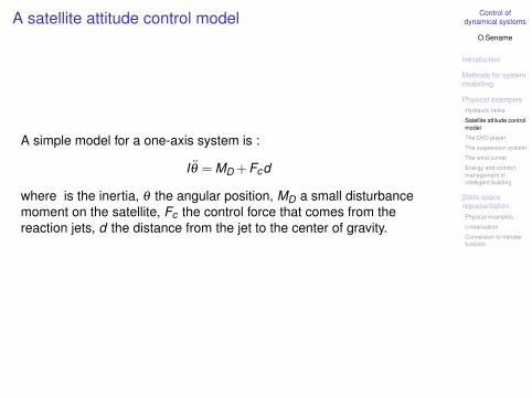
A satellite attitude control model

A simple model for a one-axis system is :

Iθ = MD + Fcd

where is the inertia, θ the angular position, MD a small disturbancemoment on the satellite, Fc the control force that comes from thereaction jets, d the distance from the jet to the center of gravity.


O.Sename

Introduction




The DVD player


The wind tunnel



Linearisation


the DVD player


O.Sename

Introduction




The DVD player


The wind tunnel



Linearisation


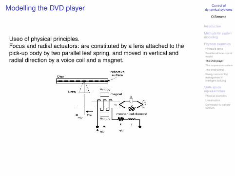
Modelling the DVD player

Useo of physical principles.Focus and radial actuators: are constituted by a lens attached to thepick-up body by two parallel leaf spring, and moved in vertical andradial direction by a voice coil and a magnet.


O.Sename

Introduction




The DVD player


The wind tunnel



Linearisation


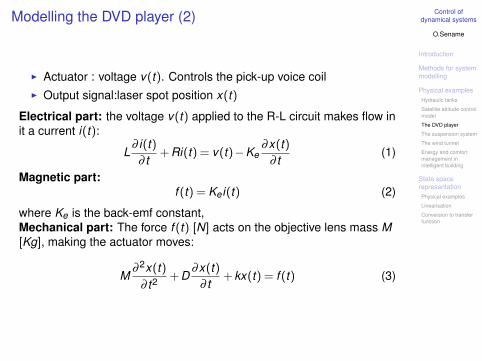
Modelling the DVD player (2)

I Actuator : voltage v(t). Controls the pick-up voice coilI Output signal:laser spot position x(t)

Electrical part: the voltage v(t) applied to the R-L circuit makes flow init a current i(t):

L∂ i(t)

∂ t+ Ri(t) = v(t)−Ke

∂x(t)∂ t

(1)

Magnetic part:f (t) = Ke i(t) (2)

where Ke is the back-emf constant,Mechanical part: The force f (t) [N] acts on the objective lens mass M[Kg], making the actuator moves:

M∂ 2x(t)

∂ t2 + D∂x(t)

∂ t+ kx(t) = f (t) (3)


O.Sename

Introduction




The DVD player


The wind tunnel



Linearisation


Data of the DVD player 1

Table: Values of the physical parameters of Pick-up 1 (for focus and trackingactuators), from Pioneer.

Name Description Value Focus Value TrackingR DC resistance of coil 5.4±1.1 Ω 5.9±1.2 ΩL Inductance of coil 15±6 µH 9±6 µHM Moving mass 0.7 g 0.7 g

SDC DC Sensitivity 2.69 mm/V 0.63 mm/Vf0 Resonance frequency 30±7 Hz 47±7 Hz

QdB Resonance peak ≤ 15 dB ≤ 15 dB


O.Sename

Introduction




The DVD player


The wind tunnel



Linearisation


Data of the DVD player 2

Table: Values of the physical parameters of Pick-up 2 (for focus and trackingactuators), from Sanyo

Name Description Value Focus Value TrackingR DC resistance of coil 6.5±1 Ω 6.5±1 ΩL Inductance of coil 25±6 µH 18±6 µHM Moving mass 0.33 g 0.33 g

SDC DC Sensitivity 0.94 mm/V 0.27 mm/Vf0 Resonance frequency 52±7 Hz 52±7 Hz

QdB Resonance peak ≤ 20 dB ≤ 20 dB


O.Sename

Introduction




The DVD player


The wind tunnel



Linearisation


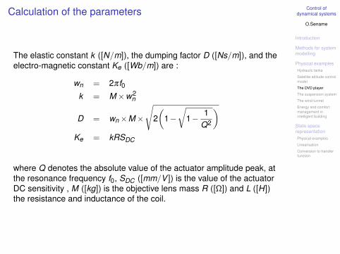
Calculation of the parameters

The elastic constant k ([N/m]), the dumping factor D ([Ns/m]), and theelectro-magnetic constant Ke ([Wb/m]) are :

wn = 2πf0k = M×w2

n

D = wn×M×

√2(

1−√

1− 1Q2

)Ke = kRSDC

where Q denotes the absolute value of the actuator amplitude peak, atthe resonance frequency f0, SDC ([mm/V ]) is the value of the actuatorDC sensitivity , M ([kg]) is the objective lens mass R ([Ω]) and L ([H])the resistance and inductance of the coil.


O.Sename

Introduction




The DVD player


The wind tunnel



Linearisation


Calculation of the transfer function

Electrical part:

I(s) =1

Ls + R[V (s)−KesX (s)] (4)

Magnetic part:F (s) = KeI(s) (5)

Mechanical part:X (s)

F (s)=

1Ms2 + Ds + k

(6)

Combining these equations , it leads

H(s) =X (s)

V (s)=

KeML

s3 +

(RL + D

M

)s2 +

(DRML + k

M + K 2e

ML

)s + kR

ML

(7)


O.Sename

Introduction




The DVD player


The wind tunnel



Linearisation


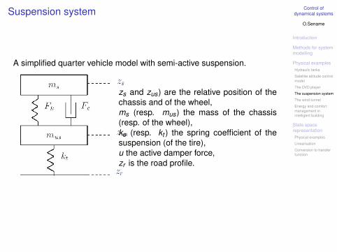
Suspension system

A simplified quarter vehicle model with semi-active suspension.

zs and zus) are the relative position of thechassis and of the wheel,ms (resp. mus) the mass of the chassis(resp. of the wheel),ks (resp. kt ) the spring coefficient of thesuspension (of the tire),u the active damper force,zr is the road profile.


O.Sename

Introduction




The DVD player


The wind tunnel



Linearisation


Suspension system (2)

The mechanical equations are:ms zs = −Fk (zdef )−Fc(zdef )

mus zus = Fk (zdef ) + Fc(zdef )−kt (zus−zr )zdef ∈

[zdef zdef

] (8)

where Fk (zdef ) and Fc(zdef ) (with zdef = zs−zus and zdef = zs− zus)are the nonlinear forces provided by the spring and damperrespectively.

−0.1 −0.05 0 0.05−4000

−3000

−2000

−1000

0

1000

2000

3000

4000Stifness coefficient

zdef

[m]

F k [N]

−1 −0.5 0 0.5 1−1000

−500

0

500

1000

1500Damping coefficient

z’def

[m/s]

F c [N]

Figure: Nonlinear forces provided by the Spring (left) and the Damper (right).


O.Sename

Introduction




The DVD player


The wind tunnel



Linearisation


Suspension system (3)

The involved model parameters have been identified on a "RenaultMégane Coupé" car and are given below.

Symbol Value Descriptionms 315kg sprung massmus 37.5kg unsprung massk 29500N/m suspension linearized stiffnessc 1500N/m/s suspension linearized dampingkp 210000N/m tire stiffness[zdef ,zdef ] [−8,6]cm suspension’s deflection limits

Table: Parameters model of a "Renault Mégane Coupé".


O.Sename

Introduction




The DVD player


The wind tunnel



Linearisation


A wind tunnel

Objective: feedback control of the Mach number in a wind tunnel(NASA)In steady-state operating conditions (some constant fan speed, liquidnitrogen injection rate, and gaseous-nitrogen vent rate), the dynamicresponse of the Mach number perturbations δM to small perturbationsin the guide vane angle actuator δθA

τδM(t) + δM(t) = kδθ(t−h)

δ θ(t) + 2ξ ωδ θ(t) + ω2δθ(t) = ω

2δθA(t)

δθ(t) is the guide vane angle.Time-delay h : transportation time between the guide vanes of the fanand the test section of the tunnelh varies as a function of the temperature and is such that0.288≤ h ≥ 0.455s.


O.Sename

Introduction




The DVD player


The wind tunnel



Linearisation


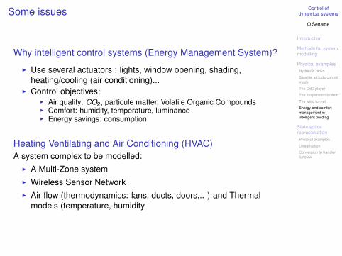
Some issues

Why intelligent control systems (Energy Management System)?

I Use several actuators : lights, window opening, shading,heating/cooling (air conditioning)...

I Control objectives:I Air quality: CO2, particule matter, Volatile Organic CompoundsI Comfort: humidity, temperature, luminanceI Energy savings: consumption

Heating Ventilating and Air Conditioning (HVAC)A system complex to be modelled:

I A Multi-Zone systemI Wireless Sensor NetworkI Air flow (thermodynamics: fans, ducts, doors,.. ) and Thermal

models (temperature, humidity


O.Sename

Introduction




The DVD player


The wind tunnel



Linearisation


Room temperature

L’équation fondamentale représentant la variation de température depart et d’autres d’un mur est la suivante:

ρ.cv .VdTdt

=λwall∆x

.A.(Tout −T ) + Qsources (9)

où

T (K ) température de la pièceTout (K ) température extérieure

cv (J/kgK ) capacité thermique de l’air à volume constant = 719cp (J/kgK ) capacité thermique de l’air à pression constante = 1010

V (m3) Volume de la pièceρ (kg/m3) densité de l’air = 1.169

∆x (m) épaisseurA (m2) Surface du mur

Qsources Sources (extérieures + contrôle)

Les coefficients de conductivité λwall dépendent des matériauxcomposant les murs, et sont donnés :


O.Sename

Introduction




The DVD player


The wind tunnel



Linearisation


General dynamical system

Many dynamical systems can be represented by Ordinary DifferentialEquations (ODE) as

x(t) = f ((x(t),u(t), t), x(0) = x0

y(t) = g((x(t),u(t), t)(10)

where f and g are non linear functions.


O.Sename

Introduction




The DVD player


The wind tunnel



Linearisation


Definition of state space representations

A continuous-time LINEAR state space system is given as :x(t) = Ax(t) + Bu(t), x(0) = x0

y(t) = Cx(t) + Du(t)(11)

I x(t) ∈ Rn is the system state (vector of state variables),I u(t) ∈ Rm the control inputI y(t) ∈ Rp the measured outputI A, B, C and D are real matrices of appropriate dimensionsI x0 is the initial condition.

n is the order of the state space representation.Matlab : ss(A,B,C,D) creates a SS object SYSrepresenting a continuous-time state-space model


O.Sename

Introduction




The DVD player


The wind tunnel



Linearisation


Height control of a single Tank

In steady state : Qe = Q0, H = H0Consider the variations qe,qs,h around the steady state as:Qe = Q0 + qe; Qs = Q0 + qs; H = H0 + h.This leads to the equation :

Sdhdt

= qe−kt (√

H0 + h−√

H0)

Using the first order approximation (1 + x)α = 1 + αx , it leads

Sdhdt

= qeh

Denoting the state variable x = h, the control input u = qe, the outputy = h, we get

x = Ax + Bu (12)

y = Cx (13)

with A =− kt2√

H0, B = 1

S and C = 1.


O.Sename

Introduction




The DVD player


The wind tunnel



Linearisation


Some exampes

Suspension systemChoose the state variables and give the state space representation ofthe system, with input zr (not controlled) and output zs−zus or zs

SatelliteChoose the state variables and give the state space representation ofthe system, with controlled input Fc , disturbance input MD and output θ .


O.Sename

Introduction




The DVD player


The wind tunnel



Linearisation


A wind tunnel

In steady-state operating conditions (fan speed, liquid nitrogen injectionrate and gaseous-nitrogen vent rate) the dynamic response of the Machnumber is given by the following system:

x(t) =

−0.5091 0 00 0 10 −36 −9.6

x(t)

+

0 −0.005956 00 0 00 0 0

x(t−h)

+

00

36

u(t) +

001

w(t)

y(t) =[

1 0 0]x(t) + w(t)

z(t) =[

1 1 1]x(t)

x(t) = φ(t); t ∈ [−h,0]

where h = 0.33sec., x1 is the Mach number, x2 is the guide vane angleand x3 = x2.


O.Sename

Introduction




The DVD player


The wind tunnel



Linearisation


Example : Wind turbine

An complete model (ADAMS) includes 193 DOFs.


O.Sename

Introduction




The DVD player


The wind tunnel



Linearisation


Some important issues

I A complete ADAMS model includes 193 DOFs to represent fullyflexible tower, drive-train, and blade components⇒ simulationmodel

I Different operating conditions according to the wind speedI Control objectives: maximize power , enhance damping in the first

drive train torsion mode, design a smooth transition differentmodes

I A Generator torque controller to enhance drive train torsiondamping in Regions 2 and 3

I The control model is obtained by linearisation of a non linearelectro-mechanical model:

x(t) = Ax(t) + Bu(t) + Ed(t)y(t) = Cx(t)

where x1 = rotor-speed x2 = drive-train torsion spring force, x3=rotational generator speedu = generator torque, d : wind speed


O.Sename

Introduction




The DVD player


The wind tunnel



Linearisation


More generally

Reformulate Nth-order differential equation into N simultaneousfirst-order differential equations

dnydtn + an−1

dn−1ydtn−1 + . . .+ a1y + a0y = f

Define the state variables :

x1 = ..., ,x2 = ...., , . . .xn = ...,

and give the according state space representation.Remark : Knowledge of state variables allows one to determine everypossible output of the system


O.Sename

Introduction




The DVD player


The wind tunnel



Linearisation


Linearisation


O.Sename

Introduction




The DVD player


The wind tunnel



Linearisation


LinearisationThe linearisation can be done around an equilibrium point or around aparticular point defined by:

xeq(t) = f ((xeq(t),ueq(t), t), givenxeq(0)

yeq(t) = g((xeq(t),ueq(t), t)(14)

Definingx = x −xeq , u = u−ueq , y = y −yeq

this leads to a linear state space representation of the system, aroundthe equilibrium point:

˙x(t) = Ax(t) + Bu(t),

y(t) = Cx(t) + Du(t)(15)

with A = ∂ f∂x |x=xeq ,u=ueq , B = ∂ f

∂u |x=xeq ,u=ueq ,

C = ∂g∂x |x=xeq ,u=ueq and D = ∂g

∂u |x=xeq ,u=ueq

Usual caseUsually an equilibrium point satisfies:

0 = f ((xeq(t),ueq(t), t) (16)

For the pendulum, we can choose y = θ = f = 0.


O.Sename

Introduction




The DVD player


The wind tunnel



Linearisation


Linear systems : transfer function


O.Sename

Introduction




The DVD player


The wind tunnel



Linearisation


Equivalence transfer function - state space representation

Consider a linear system given by:x(t) = Ax(t) + Bu(t), x(0) = x0y(t) = Cx(t) + Du(t) (17)

Using the Laplace transform (and assuming zero initial conditionx0 = 0), (17) becomes:

s.x(s) = Ax(s) + Bu(s) ⇒ (s.In−A)x(s) = Bu(s)

Then the transfer function matrix of system (17) is given by

G(s) = C(sIn−A)−1B + D =N(s)

D(s)(18)

Matlab: if SYS is an SS object, then tf(SYS) gives the associatedtransfer matrix. Equivalent to tf(N,D)

Documents

Methods for analysis and control of dynamical systems - GIPSA-lab