Spectral Calibration of the Fluorescence Telescopes of

the Pierre Auger Observatory

A. Aabbz, P. Abreubq, M. Agliettaax,aw, I. Al Samaraiaf,I.F.M. Albuquerquer, I. Allekottea, A. Almelah,k, J. Alvarez Castillobm,J. Alvarez-Munizby, G.A. Anastasiao,aq, L. Anchordoquicf, B. Andradah,S. Andringabq, C. Aramoau, F. Arquerosbw, N. Arsenebs, H. Asoreya,aa,

P. Assisbq, J. Aublinaf, G. Avilai,j, A.M. Badescubt, A. Balaceanubr,F. Barbatobe, R.J. Barreira Luzbq, J.J. Beattyck, K.H. Beckerah,

J.A. Bellidol, C. Beratag, M.E. Bertainabg,aw, P.L. Biermanncp, J. Biteauae,S.G. Blaessl, A. Blancobq, J. Blazekac, C. Bleveba,as, M. Bohacovaac,

D. Boncioliaq,cr, C. Bonifazix, N. Borodaibn, A.M. Bottih,aj, J. Brackcv,I. Brancusbr, T. Bretzal, A. Bridgemanaj, F.L. Briechleal, P. Buchholzan,

A. Buenobx, S. Buitinkbz, M. Buscemibc,ar, K.S. Caballero-Morabk,L. Caccianigabd, A. Canciok,h, F. Canforabz, L. Carametebs, R. Carusobc,ar,A. Castellinaax,aw, F. Catalanir, G. Cataldias, L. Cazonbq, A.G. Chavezbl,J.A. Chinellatos, J. Chudobaac, R.W. Clayl, A. Cobosh, R. Colalillobe,au,

A. Colemancl, L. Collicaaw, M.R. Colucciaba,as, R. Conceicaobq,G. Consolatiat,ay, F. Contrerasi,j, M.J. Cooperl, S. Coutucl, C.E. Covaultcd,

J. Cronincm, S. D’Amicoaz,as, B. Daniels, S. Dassoe,c, K. Daumilleraj,B.R. Dawsonl, R.M. de Almeidaz, S.J. de Jongbz,cb, G. De Maurobz,

J.R.T. de Mello Netox,y, I. De Mitriba,as, J. de Oliveiraz, V. de Souzaq,J. Debatinaj, O. Delignyae, M.L. Dıaz Castros, F. Diogobq, C. Dobrigkeits,

J.C. D’Olivobm, Q. Dorostian, R.C. dos Anjosw, M.T. Dovad,A. Dundovicam, J. Ebrac, R. Engelaj, M. Erdmannal, M. Erfanian,

C.O. Escobarct, J. Espadanalbq, A. Etchegoyenh,k, H. Falckebz,cc,cb,J. Farmercm, G. Farrarci, A.C. Fauths, N. Fazzinict, F. Fenubg,aw, B. Fickch,

J.M. Figueirah, A. Filipcicbu,bv, O. Fratubt, M.M. Freiref, T. Fujiicm,A. Fusterh,k, R. Gaioraf, B. Garcıag, D. Garcia-Pintobw, F. Gatecs,

H. Gemmekeak, A. Gherghel-Lascubr, U. Giaccarix, M. Giammarchiat,M. Gillerbo, D. G lasbp, C. Glaseral, G. Golupa, M. Gomez Berissoa,P.F. Gomez Vitalei,j, N. Gonzalezh,aj, B. Gookincv, A. Gorgiax,aw,

P. Gorhamcw, A.F. Grilloaq, T.D. Grubbl, F. Guarinobe,au, G.P. Guedest,R. Hallidaycd, M.R. Hampelh, P. Hansend, D. Hararia, T.A. Harrisonl,

∗Corresponding Author. E-mail address: auger spokespersons@fnal.gov

Preprint submitted to Elsevier September 7, 2017

arX

iv:1

709.

0153

7v1

[ast

ro-p

h.IM

] 5

Sep

2017

FERMILAB-PUB-17-355 ACCEPTED

This document was prepared by Pierre Auger collaboration using the resources of the Fermi National Accelerator Laboratory (Fermilab), a U.S. Department of Energy, Office of Science, HEP User Facility. Fermilab is managed by Fermi Research Alliance, LLC (FRA), acting under Contract No. DE-AC02-07CH11359.

J.L. Hartoncv, A. Haungsaj, T. Hebbekeral, D. Heckaj, P. Heimannan,A.E. Herveai, G.C. Hilll, C. Hojvatct, E. Holtaj,h, P. Homolabn,J.R. Horandelbz,cb, P. Horvathad, M. Hrabovskyad, T. Huegeaj,

J. Hulsmanh,aj, A. Insoliabc,ar, P.G. Isarbs, I. Jandtah, J.A. Johnsence,M. Josebachuilih, J. Jurysekac, A. Kaapaah, O. Kambeitzai,

K.H. Kampertah, B. Keilhaueraj, N. Kemmerichr, E. Kemps, J. Kempal,R.M. Kieckhaferch, H.O. Klagesaj, M. Kleifgesak, J. Kleinfelleri, R. Krauseal,

N. Krohmah, D. Kuempelal, G. Kukec Mezekbv, N. Kunkaak, A. KuotbAwadaj, B.L. Lagoo, D. LaHurdcd, R.G. Langq, M. Lauscheral,R. Leguminabo, M.A. Leigui de Oliveirav, A. Letessier-Selvonaf,

I. Lhenry-Yvonae, K. Linkai, D. Lo Prestibc, L. Lopesbq, R. Lopezbh,A. Lopez Casadoby, R. Lorekcd, Q. Luceae, A. Luceroh,k, M. Malacaricm,

M. Mallamacibd,at, D. Mandatac, P. Mantschct, A.G. Mariazzid, I.C. Marism,G. Marsellaba,as, D. Martelloba,as, H. Martinezbi, O. Martınez Bravobh,

J.J. Masıas Mezac, H.J. Mathesaj, S. Mathysah, J. Matthewscg,J.A.J. Matthewscx, G. Matthiaebf,av, E. Mayotteah, P.O. Mazurct,

C. Medinace, G. Medina-Tancobm, D. Meloh, A. Menshikovak,K.-D. Merendace, S. Michalad, M.I. Michelettif, L. Middendorfal,

L. Miramontibd,at, B. Mitricabr, D. Mocklerai, S. Molleracha, F. Montanetag,C. Morelloax,aw, M. Mostafacl, A.L. Mullerh,aj, G. Mulleral, M.A. Mullers,u,

S. Mulleraj,h, R. Mussaaw, I. Naranjoa, L. Nellenbm, P.H. Nguyenl,M. Niculescu-Oglinzanubr, M. Niechciolan, L. Niemietzah, T. Niggemannal,

D. Nitzch, D. Nosekab, V. Novotnyab, L. Nozkaad, L.A. Nunezaa, L. Ochiloan,F. Oikonomoucl, A. Olintocm, M. Palatkaac, J. Pallottab, P. Papenbreerah,G. Parenteby, A. Parrabh, T. Paulcf, M. Pechac, F. Pedreiraby, J. Pekalabn,

R. Pelayobj, J. Pena-Rodriguezaa, L. A. S. Pereiras, M. Perlinh,L. Perroneba,as, C. Petersal, S. Petreraao,aq, J. Phuntsokcl, R. Piegaiac,T. Pierogaj, M. Pimentabq, V. Pirronellobc,ar, M. Platinoh, M. Plumal,C. Porowskibn, R.R. Pradoq, P. Priviteracm, M. Prouzaac, E.J. Quelb,

S. Querchfeldah, S. Quinncd, R. Ramos-Pollanaa, J. Rautenbergah,D. Ravignanih, J. Ridkyac, F. Riehnbq, M. Rissean, P. Ristorib, V. Rizibb,aq,

W. Rodrigues de Carvalhor, G. Rodriguez Fernandezbf,av, J. RodriguezRojoi, D. Rogozinaj, M.J. Roncoronih, M. Rothaj, E. Rouleta, A.C. Roveroe,

P. Ruehlan, S.J. Saffil, A. Saftoiubr, F. Salamidabb,aq, H. Salazarbh,A. Salehbv, F. Salesa Greuscl, G. Salinaav, F. Sanchezh, P. Sanchez-Lucasbx,E.M. Santosr, E. Santosh, F. Sarazince, R. Sarmentobq, C. Sarmiento-Canoh,

R. Satoi, M. Schauerah, V. Scherinias, H. Schieleraj, M. Schimpah,D. Schmidtaj,h, O. Scholtenca,cq, P. Schovanekac, F.G. Schroderaj,

2

S. Schroderah, A. Schulzai, J. Schumacheral, S.J. Sciuttod, A. Segretoap,ar,A. Shadkamcg, R.C. Shellardn, G. Siglam, G. Sillih,aj, O. Simacu,

A. Smia lkowskibo, R. Smıdaaj, G.R. Snowcn, P. Sommerscl, S. Sonntagan,R. Squartinii, D. Stancabr, S. Stanicbv, J. Stasielakbn, P. Stassiag,

M. Stolpovskiyag, F. Strafellaba,as, A. Streichai, F. Suarezh,k, M. SuarezDuranaa, T. Sudholzl, T. Suomijarviae, A.D. Supanitskye, J. Supıkad,

J. Swaincj, Z. Szadkowskibp, A. Taboadaai, O.A. Tabordaa, V.M. Theodoros,C. Timmermanscb,bz, C.J. Todero Peixotop, L. Tomankovaaj, B. Tomebq,G. Torralba Elipeby, P. Travnicekac, M. Trinibv, R. Ulrichaj, M. Ungeraj,

M. Urbanal, J.F. Valdes Galiciabm, I. Valinoby, L. Valorebe,au, G. van Aarbz,P. van Bodegoml, A.M. van den Bergca, A. van Vlietbz, E. Varelabh,B. Vargas Cardenasbm, G. Varnercw, R.A. Vazquezby, D. Vebericaj,

C. Venturay, I.D. Vergara Quisped, V. Verziav, J. Vichaac, L. Villasenorbl,S. Vorobiovbv, H. Wahlbergd, O. Wainbergh,k, D. Walzal, A.A. Watsonco,

M. Weberak, A. Weindlaj, L. Wienckece, H. Wilczynskibn, M. Wirtzal,D. Wittkowskiah, B. Wundheilerh, L. Yangbv, A. Yushkovh, E. Zasby,D. Zavrtanikbv,bu, M. Zavrtanikbu,bv, A. Zepedabi, B. Zimmermannak,

M. Ziolkowskian, Z. Zongae, F. Zuccarellobc,ar, The Pierre AugerCollaboration∗

aCentro Atomico Bariloche and Instituto Balseiro (CNEA-UNCuyo-CONICET), SanCarlos de Bariloche, Argentina

bCentro de Investigaciones en Laseres y Aplicaciones, CITEDEF and CONICET, VillaMartelli, Argentina

cDepartamento de Fısica and Departamento de Ciencias de la Atmosfera y los Oceanos,FCEyN, Universidad de Buenos Aires and CONICET, Buenos Aires, ArgentinadIFLP, Universidad Nacional de La Plata and CONICET, La Plata, Argentina

eInstituto de Astronomıa y Fısica del Espacio (IAFE, CONICET-UBA), Buenos Aires,Argentina

fInstituto de Fısica de Rosario (IFIR) – CONICET/U.N.R. and Facultad de CienciasBioquımicas y Farmaceuticas U.N.R., Rosario, Argentina

gInstituto de Tecnologıas en Deteccion y Astropartıculas (CNEA, CONICET, UNSAM),and Universidad Tecnologica Nacional – Facultad Regional Mendoza

(CONICET/CNEA), Mendoza, ArgentinahInstituto de Tecnologıas en Deteccion y Astropartıculas (CNEA, CONICET, UNSAM),

Buenos Aires, ArgentinaiObservatorio Pierre Auger, Malargue, Argentina

jObservatorio Pierre Auger and Comision Nacional de Energıa Atomica, Malargue,Argentina

kUniversidad Tecnologica Nacional – Facultad Regional Buenos Aires, Buenos Aires,Argentina

lUniversity of Adelaide, Adelaide, S.A., Australia

3

mUniversite Libre de Bruxelles (ULB), Brussels, BelgiumnCentro Brasileiro de Pesquisas Fisicas, Rio de Janeiro, RJ, Brazil

oCentro Federal de Educacao Tecnologica Celso Suckow da Fonseca, Nova Friburgo,Brazil

pUniversidade de Sao Paulo, Escola de Engenharia de Lorena, Lorena, SP, BrazilqUniversidade de Sao Paulo, Instituto de Fısica de Sao Carlos, Sao Carlos, SP, Brazil

rUniversidade de Sao Paulo, Instituto de Fısica, Sao Paulo, SP, BrazilsUniversidade Estadual de Campinas, IFGW, Campinas, SP, Brazil

tUniversidade Estadual de Feira de Santana, Feira de Santana, BraziluUniversidade Federal de Pelotas, Pelotas, RS, Brazil

vUniversidade Federal do ABC, Santo Andre, SP, BrazilwUniversidade Federal do Parana, Setor Palotina, Palotina, Brazil

xUniversidade Federal do Rio de Janeiro, Instituto de Fısica, Rio de Janeiro, RJ, BrazilyUniversidade Federal do Rio de Janeiro (UFRJ), Observatorio do Valongo, Rio de

Janeiro, RJ, BrazilzUniversidade Federal Fluminense, EEIMVR, Volta Redonda, RJ, Brazil

aaUniversidad Industrial de Santander, Bucaramanga, ColombiaabCharles University, Faculty of Mathematics and Physics, Institute of Particle and

Nuclear Physics, Prague, Czech RepublicacInstitute of Physics of the Czech Academy of Sciences, Prague, Czech Republic

adPalacky University, RCPTM, Olomouc, Czech RepublicaeInstitut de Physique Nucleaire d’Orsay (IPNO), Universite Paris-Sud, Univ.

Paris/Saclay, CNRS-IN2P3, Orsay, FranceafLaboratoire de Physique Nucleaire et de Hautes Energies (LPNHE), Universites Paris

6 et Paris 7, CNRS-IN2P3, Paris, FranceagLaboratoire de Physique Subatomique et de Cosmologie (LPSC), Universite

Grenoble-Alpes, CNRS/IN2P3, Grenoble, FranceahBergische Universitat Wuppertal, Department of Physics, Wuppertal, Germany

aiKarlsruhe Institute of Technology, Institut fur Experimentelle Kernphysik (IEKP),Karlsruhe, Germany

ajKarlsruhe Institute of Technology, Institut fur Kernphysik, Karlsruhe, GermanyakKarlsruhe Institute of Technology, Institut fur Prozessdatenverarbeitung und

Elektronik, Karlsruhe, GermanyalRWTH Aachen University, III. Physikalisches Institut A, Aachen, Germany

amUniversitat Hamburg, II. Institut fur Theoretische Physik, Hamburg, GermanyanUniversitat Siegen, Fachbereich 7 Physik – Experimentelle Teilchenphysik, Siegen,

GermanyaoGran Sasso Science Institute (INFN), L’Aquila, Italy

apINAF – Istituto di Astrofisica Spaziale e Fisica Cosmica di Palermo, Palermo, ItalyaqINFN Laboratori Nazionali del Gran Sasso, Assergi (L’Aquila), Italy

arINFN, Sezione di Catania, Catania, ItalyasINFN, Sezione di Lecce, Lecce, Italy

atINFN, Sezione di Milano, Milano, ItalyauINFN, Sezione di Napoli, Napoli, Italy

avINFN, Sezione di Roma ”Tor Vergata”, Roma, Italy

4

awINFN, Sezione di Torino, Torino, ItalyaxOsservatorio Astrofisico di Torino (INAF), Torino, Italy

ayPolitecnico di Milano, Dipartimento di Scienze e Tecnologie Aerospaziali , Milano, ItalyazUniversita del Salento, Dipartimento di Ingegneria, Lecce, Italy

baUniversita del Salento, Dipartimento di Matematica e Fisica “E. De Giorgi”, Lecce,Italy

bbUniversita dell’Aquila, Dipartimento di Scienze Fisiche e Chimiche, L’Aquila, ItalybcUniversita di Catania, Dipartimento di Fisica e Astronomia, Catania, Italy

bdUniversita di Milano, Dipartimento di Fisica, Milano, ItalybeUniversita di Napoli ”Federico II”, Dipartimento di Fisica “Ettore Pancini“, Napoli,

ItalybfUniversita di Roma “Tor Vergata”, Dipartimento di Fisica, Roma, Italy

bgUniversita Torino, Dipartimento di Fisica, Torino, ItalybhBenemerita Universidad Autonoma de Puebla, Puebla, Mexico

biCentro de Investigacion y de Estudios Avanzados del IPN (CINVESTAV), Mexico,D.F., Mexico

bjUnidad Profesional Interdisciplinaria en Ingenierıa y Tecnologıas Avanzadas delInstituto Politecnico Nacional (UPIITA-IPN), Mexico, D.F., Mexico

bkUniversidad Autonoma de Chiapas, Tuxtla Gutierrez, Chiapas, MexicoblUniversidad Michoacana de San Nicolas de Hidalgo, Morelia, Michoacan, Mexico

bmUniversidad Nacional Autonoma de Mexico, Mexico, D.F., MexicobnInstitute of Nuclear Physics PAN, Krakow, Poland

boUniversity of Lodz, Faculty of Astrophysics, Lodz, PolandbpUniversity of Lodz, Faculty of High-Energy Astrophysics, Lodz, Poland

bqLaboratorio de Instrumentacao e Fısica Experimental de Partıculas – LIP and InstitutoSuperior Tecnico – IST, Universidade de Lisboa – UL, Lisboa, Portugal

br“Horia Hulubei” National Institute for Physics and Nuclear Engineering,Bucharest-Magurele, Romania

bsInstitute of Space Science, Bucharest-Magurele, RomaniabtUniversity Politehnica of Bucharest, Bucharest, Romania

buExperimental Particle Physics Department, J. Stefan Institute, Ljubljana, SloveniabvCenter for Astrophysics and Cosmology (CAC), University of Nova Gorica, Nova

Gorica, SloveniabwUniversidad Complutense de Madrid, Madrid, Spain

bxUniversidad de Granada and C.A.F.P.E., Granada, SpainbyUniversidad de Santiago de Compostela, Santiago de Compostela, Spain

bzIMAPP, Radboud University Nijmegen, Nijmegen, The NetherlandscaKVI – Center for Advanced Radiation Technology, University of Groningen,

Groningen, The NetherlandscbNationaal Instituut voor Kernfysica en Hoge Energie Fysica (NIKHEF), Science Park,

Amsterdam, The NetherlandsccStichting Astronomisch Onderzoek in Nederland (ASTRON), Dwingeloo, The

NetherlandscdCase Western Reserve University, Cleveland, OH, USA

ceColorado School of Mines, Golden, CO, USA

5

cfDepartment of Physics and Astronomy, Lehman College, City University of New York,Bronx, NY, USA

cgLouisiana State University, Baton Rouge, LA, USAchMichigan Technological University, Houghton, MI, USA

ciNew York University, New York, NY, USAcjNortheastern University, Boston, MA, USAckOhio State University, Columbus, OH, USA

clPennsylvania State University, University Park, PA, USAcmUniversity of Chicago, Enrico Fermi Institute, Chicago, IL, USA

cnUniversity of Nebraska, Lincoln, NE, USAcoSchool of Physics and Astronomy, University of Leeds, Leeds, United Kingdom

cpMax-Planck-Institut fur Radioastronomie, Bonn, Germanycqalso at Vrije Universiteit Brussels, Brussels, Belgium

crnow at Deutsches Elektronen-Synchrotron (DESY), Zeuthen, GermanycsSUBATECH, Ecole des Mines de Nantes, CNRS-IN2P3, Universite de Nantes, France

ctFermi National Accelerator Laboratory, USAcuUniversity of Bucharest, Physics Department, Bucharest, Romania

cvColorado State University, Fort Collins, COcwUniversity of Hawaii, Honolulu, HI, USA

cxUniversity of New Mexico, Albuquerque, NM, USA

Abstract

We present a novel method to measure precisely the relative spectral re-sponse of the fluorescence telescopes of the Pierre Auger Observatory. Weused a portable light source based on a xenon flasher and a monochromatorto measure the relative spectral efficiencies of eight telescopes in steps of 5nm from 280 nm to 440 nm. Each point in a scan had approximately 2 nmFWHM out of the monochromator. Different sets of telescopes in the obser-vatory have different optical components, and the eight telescopes measuredrepresent two each of the four combinations of components represented inthe observatory. We made an end-to-end measurement of the response fromdifferent combinations of optical components, and the monochromator setupallowed for more precise and complete measurements than our previous multi-wavelength calibrations. We find an overall uncertainty in the calibration ofthe spectral response of most of the telescopes of 1.5% for all wavelengths;the six oldest telescopes have larger overall uncertainties of about 2.2%. Wealso report changes in physics measureables due to the change in calibration,which are generally small.

6

Keywords: Auger Observatory, Nitrogen Fluorescence, Extensive AirShower, Calibration

1. Introduction

The Pierre Auger Observatory [1] has been designed to study the originand the nature of ultra high-energy cosmic rays, which have energies above1018 eV. The construction of the complete observatory following the originaldesign finished in 2008. The observatory is located in Malargue, Argentina,and consists of two complementary detector systems, which provide inde-pendent information on the cosmic ray events. Extensive Air Showers (EAS)initiated by cosmic rays in the Earth’s atmosphere are measured by the Sur-face Detector (SD) and the Fluorescence Detector (FD). The SD is composedof 1660 water Cherenkov detectors located mostly on a triangular array of1.5 km spacing covering an area of roughly 3000 km2. The SD measures theEAS secondary particles reaching ground level [2]. The FD is designed tomeasure the nitrogen fluorescence light produced in the atmosphere by theEAS secondary particles. The FD is composed of 27 telescopes overlookingthe SD array from four sites, Los Leones (LL), Los Morados (LM), LomaAmarilla (LA), and Coihueco (CO) [3]. The SD takes data continuously, butthe FD operates only on clear nights, and care is taken to avoid exposure totoo much moonlight.

The energy of the primary cosmic ray is a key measurable for the science ofthe observatory, and the FD measurement of the energy, with lower indepen-dent systematic uncertainties, is used to calibrate the SD energy scale usingevents observed by both detectors. The work described here explains how theFD calibration at wavelengths across the nitrogen fluorescence spectrum hasrecently been improved, resulting in smaller related systematic uncertainties.

The buildings at the four FD sites each have six independent telescopes,and each telescope has a 30°× 30° field of view, leading to a 180° coverage inazimuth and from 2° to 32° in elevation at each building. Additionally, threespecialized telescopes called HEAT [4] are located near Coihueco to overlooka portion of the SD array at higher elevations, from 32° to 62°, to registerEAS of lower energies. All these telescopes are housed in climate-controlledbuildings, isolated from dust and day light. The layout of the observatory isshown schematically in Figure 1.

Each FD telescope is composed of several optical components as shown inFigure 2: a 2.2 m aperture diaphragm, a UV filter to reduce the background

7

Figure 1: A schematic of the Pierre Auger Observatory where each black dot is a waterCherenkov detector. Locations of the fluorescence telescopes are shown along the perimeterof the surface detector array, where the blue lines indicate their individual field of view.The field of view of the HEAT telescopes are indicated with red lines.

light, a Schmidt corrector annulus, a 3.5 m × 3.5 m tessellated sphericalmirror, and a camera formed by an array of 440 hexagonal photomultipliers(PMT) each with a field of view of 1.5° full angle. Each PMT has a lightconcentrator approximating a hexagonal Winston cone to reduce dead spacesbetween PMTs [3].

The energy calibration of the data [5, 6] for the Pierre Auger Observa-tory, including events observed by the SD only, relies on the calibration ofthe FD. Events observed by both FD and SD provide the link from the FD,which is absolutely calibrated, to the SD data. To calibrate the FD threedifferent procedures are performed: the absolute [7], the relative [8], and thespectral (or multi-wavelength) calibrations [9]. We focus here on the spectralcalibration, which is a relative measurement that relates the absolute cali-bration performed at 365 nm to wavelengths across the nitrogen fluorescencespectrum, which is shown in Figure 3.

To perform this measurement the drum-shaped portable light source usedfor the absolute calibration [7] was adapted to emit UV light across thewavelength range of interest. The drum light source is designed to uniformlyilluminate all 440 PMTs in a single camera simultaneously when it is placedat the aperture of the FD telescope, enabling the end-to-end calibration.

The FD response as a function of wavelength was initially calculated as

8

Figure 2: The optical components of an individual fluorescence telescope.

a convolution of separate reflection or transmission measurements of eachoptical component used in the first Los Leones telescopes [11]. The first end-to-end spectral calibration of the FD was performed using the drum lightsource with a xenon flasher and filter wheel to provide five points across theFD wavelength response [9]. This measurement represented an improvementfor the energy estimation of all events observed by the Pierre Auger Obser-vatory as it has been shown to increase the reconstructed energy of eventsby nearly 4% for all energies [12]. However, that result has two limitations:first, the differences in FD optical components were not measured since onlyone telescope was calibrated; and second, determining the FD spectral re-sponse curve using only five points involved a complicated fitting procedure,and was particularly difficult considering the large width of the filters, whichresulted in relatively large systematic uncertainties.

The aim of the work described in this paper was to measure the FDefficiency at many points across the nitrogen fluorescence spectrum with areduced wavelength bite at each point, and to do it at enough telescopesto cover the different combinations of optical components making up all thetelescopes within the Auger Observatory. The spectral calibration describedhere proceeds in three steps. First, the relative drum emission spectrum ismeasured in the dark hall lab in Malargue with a specific calibration PMT,called the “Lab-PMT”, observing the drum at a large distance, in a simi-

9

Figure 3: The nitrogen fluorescence spectrum as measured by the AIRFLY collaboration[10] showing the 21 major transitions.

lar fashion to the absolute calibration of the drum; see [7] and explanatorydrawings therein. Knowing the intensity of the drum at each wavelength, wenext measure the response of the FD telescopes to the output of the multi-wavelength drum over the course of several nights, while recording data froma monitoring photodiode (PD) exposed to the narrow-band light at each pointto ensure knowledge of the relative drum spectrum. Finally, the FD telescoperesponse is normalized by the measured relative drum emission spectrum atevery wavelength, and we evaluate the associated systematic uncertainties inthe final calculation of the efficiency.

This following sections describe the measurements and analysis of datataken during March 2014: FD optical components in section 2; the new drumlight source in section 3; measurements of the drum light source spectrumin section 4; calibrations performed at the FD telescopes in section 5; FDefficiency as a function of wavelength in section 6; and final calibration resultsin section 7. Effects on physics measurables due to changing calibrations arediscussed in section 8.

2. Optical Components of the Fluorescence Telescopes

There are two types of mirrors used in the telescopes, and the glass usedfor the corrector rings was produced using two different glass-making proce-dures. The 12 mirrors at Los Leones and Los Morados are aluminum with a2 mm AlMgSiO5 layer glued on as the reflective surface, and the 12 mirrorsat Coihueco and Loma Amarilla are composed of a borosilicate glass witha 90 nm Al layer and then a 110 nm SiO2 layer (see [3] for more details).

10

Two different procedures were used to grow the borosilicate glass used inthe corrector rings, both by Schott Glass Manufactures1. One type is calledBorofloat 332, and the other is a crown glass labeled P-BK73, and the trans-mission of UV light differs for these two products.

Given the different wavelength dependencies of the above components,our aim was to measure the four combinations of mirrors and corrector ringspresent in the FDs. This meant calibrating at three of the four FD build-ings. Table 1 shows the eight telescopes we calibrated at the three FD sitesalong with which components make up each telescope. Calibration of theseeight telescopes gives a complete coverage of the different components and aduplicate measure of each combination.

Table 1: List of the FD telescopes we calibrated and their respective optical components.Calibration at these eight FD telescopes gives a complete coverage of the different compo-nents and a duplicate measure of each combination. The last column indicates all other(unmeasured) telescopes with the same optical components.

FD telescope Mirror Type Corrector Ring FDs with samecomponents

Coihueco 2 Glass BK7Coihueco 3 Glass BK7 CO2/3Coihueco 4 Glass Borofloat 33 CO1,4-6, LA,Coihueco 5 Glass Borofloat 33 HEATLos Morados 4 Aluminum Borofloat 33Los Morados 5 Aluminum Borofloat 33 LMLos Leones 3 Aluminum BK7Los Leones 4 Aluminum BK7 LL1-6

As seen in Table 1, the telescopes CO 4/5 are the only ones that havesame nominal components as those located at other FD buildings, which havedifferent construction dates. It is usualy the case that optical componentsdegrade their properties when exposed to light and ambient conditions (age-

1Schott Glass, http://www.us.schott.com/english/index.html2Borofloat, http://www.us.schott.com/borofloat/english/attribute/optical3P-BK7, http://www.schott.com/advanced_optics/us/abbe_datasheets/schott_

datasheet_all_us.pdf

11

ing), whose effect depends on exposure time. Even if FD telescopes are keptin climate-controlled buildings, an analysis of ageing follows. Regarding thespectral calibration, what has to be evaluated is the change in the spectralresponse of a given FD telescope, i.e. the shape of the response curve vswavelength. This kind of differential degradation is not obviously seen atthe FD telescopes. One way to evaluate whether there is any change in thespectral response is to track the absolute calibration done periodically at 375nm [1, 2]. The absolute calibration is scaled at any given date by using thenightly relative calibration, which is done at 470 nm [1, 2]. Because thesetwo calibrations are done at different wavelengths, any change in the spec-tral response would translate in a drift of the absolute calibration with time.In Table 2 we show the variations of the ratio (R) of absolute calibrationsperformed in 2010 and 2013, where R = (Abs2013 − Abs2010)/Abs2013, alongwith the date of finished construction for telescopes at a given building. Asseen in the table, the variations do not respond to any ageing pattern, e.g.for the oldest telescopes there is a positive variation for LL and a negativevariation for CO. Moreover, the overall effect that telescopes could have indata analysis do not change the final reconstructed energy significantly (seeFig. 49 in [1]). For these reasons, we consider that different time of telescopeconstruction do not play a role in the spectral calibration described in thispaper and, consequently, CO 4/5 can be taken as representative of LA andHEAT.

Table 2: List of FD buildings and dates when construction was finished and operationstarted. ∆t is the elapsed time until measurements done for this work (March 2014). R isthe ratio of absolute calibrations performed in 2010 and 2013 (see text).

FD building Built ∆t [yr] R [%]

Los Leones 5/2004 9.8 + 1.4Coihueco 5/2004 9.8 – 1.6Los Morados 3/2005 9.0 – 0.5Loma Amarilla 2/2007 7.1 – 0.8HEAT 9/2009 4.5

12

3. Monochromator Drum Setup

The work described in [9] was the first in-situ end-to-end measurementof the FD efficiency as a function of wavelength. It limited the measurementto only five points across the ∼150 nm wide acceptance of the FDs, and thefilters had a fairly wide spectral width, about ∼15 nm FWHM, as shown inthe bottom of Figure 4. The large spectral width led to a complicated pro-cedure of accounting for the width effects along the rising and falling edgesof the efficiency curve [9]. In addition, since there were only five measuredpoints, the resulting calibration curve had to be interpolated between thepoints, and the original piece-wise efficiency curve [11] was used as the start-ing point. In the five-point measurement [9] the efficiency was assumed to goto zero below 290 nm and above 425 nm since the filters did not extend tothese wavelengths, thus the values resulting from the piece-wise convolutionof the component efficiencies [11] were the only data for wavelengths below290 nm and above 425 nm.

Figure 4: A comparison showing the spectral width of the output of the monochromatorsampled every 5 nm (top, this work) and the notch filter spectral transmission (bottom,[9]). The y-axes are the intensity in arbitrary units for the monochromator and thenormalized transmission for the notch filters.

These reasons are the motivation for using a monochromator to select

13

the wavelengths out of a UV spectrum. A monochromator allows for a highresolution probe across the FD acceptance, and a far more detailed mea-surement can be performed. The top of Figure 4 shows the output of themonochromator in 5 nm steps from 275 nm to 450 nm with a xenon flasher asthe input, each step with a 2 nm FWHM. The xenon flasher is an ExcelitasPAX-10 model4 with improved EM noise reduction and variable flash inten-sity. The monochromator output width was chosen to provide a reasonablecompromise between wavelength resolution and the drum intensity requiredfor use at the FDs.

For the work described here, an enclosure housing the monochromatorand xenon flasher was mounted onto the rear of the drum. The enclosurewas insulated and contained a heater and associated controlling circuitry tomaintain a stable 20±2 ℃ temperature for monochromator reliability.

A custom 25.4 mm diameter aluminum tube was fabricated and attachedto the output of the monochromator; it protrudes into the interior of thedrum. At the end of the tube a 0.23 mm thick Teflon diffuser ensured thatthe illumination of the front face of the drum was uniform as measured withlong-exposure CCD images, similar to what had been measured previously[3, 13].

A photodiode (PD) was mounted near the output of the monochroma-tor, but upstream of the tube that protruded into the drum, allowing forpulse-by-pulse monitoring of the emission spectrum from the monochroma-tor. The monochromator and xenon flasher were controlled with the samecommon gateway interface (CGI) web page and calibration electronics thathave been used in the absolute calibration [7]. Scanning of the monochroma-tor, triggering of the flasher, and data acquisition from monitoring devicesand the FD were all fully automated using CGI code and cURL5 scripts overthe wireless LAN used for drum calibrations.

4. Lab Measurements and the Drum Spectrum

To characterize the drum emission as a function of wavelength, severalmeasurements were needed in the laboratory. For the one-week calibrationcampaign described here, four measurements were performed in the lab, two

4PAX-10 10-Watt Precision-Aligned Pulsed Xenon Light Source - http://www.

excelitas.com/downloads/dts_pax10.pdf5cURL Documentation - http://curl.haxx.se/

14

prior to any field work at the FD telescopes, one two days later and the lastone at the end of the week.

4.1. Drum Emission

With the automated scanning of the monochromator and data acquisi-tion we took measurements of the relative drum emission spectrum as viewedby the calibration Lab-PMT. The monitoring PD detector measured themonochromator output as described above. The setup for these measure-ments had the drum at the far end of the dark hall and the Lab-PMT insidethe darkbox in the calibration room, about 16 m away from the Teflon faceof the drum. See [7] for a detailed description of the dark hall calibrationsetup.

The average response of the Lab-PMT to 100 pulses of the drum wasrecorded as a function of wavelength from 250 nm to 450 nm, in steps of1 nm. The uncertainty in the average for a given wavelength was calculatedas the standard deviation of the mean, σDrum√

100. The solid grey line in Figure 5

shows an example of one of these spectra. We took averages of the fourspectra at each wavelength as the final measurement of the drum spectrum,which is shown in the same figure as blue dots. This final drum spectrumused measurements in steps of 5 nm corresponding to the step size used whencalibrating the FD telescopes. For wavelengths between 320 nm and 390 nm,the four measurements were generally statistically consistent. But for wave-lengths at the low and high ends of the spectrum there was disagreement;section 4.3 explains how we introduce a systematic uncertainty to accountfor this disagreement.

For each of these four spectra measured with the Lab-PMT there are datafrom the monitoring PD. The monitoring PD data were handled in the sameway; we made an average of the four spectra recorded by the PD and anassociated error based on the spread of the four measurements. These dataare shown in Figure 5 as black line and points.

4.2. Lab-PMT Quantum Efficiency

A measurement of the quantum efficiency (QE) of the Lab-PMT, whichis used to measure the relative drum emission spectrum, has to be performedto measure the relative response of a given FD telescope at different wave-lengths. The method used here is similar to what was done previously [9]except, instead of a DC deuterium lamp, we used the xenon flasher as theUV light source into the monochromator. For the work reported here we

15

Figure 5: Drum emission spectra. Solid grey line: one of the measured spectra taken withthe Lab-PMT; the line shows the average responses to 100 pulses of the drum as a functionof wavelength, in steps of 1 nm. Blue points: the averaged drum spectrum as measuredby the Lab-PMT throughout the calibration campaign; the spectrum is taken in steps of5 nm as this is what is used to measure the FD responses; error bars are the statisticaluncertainties, which are generally smaller than the plotted points. Black line and points:the averaged drum spectrum as measured by the monitoring photodiode (PD) throughoutthe calibration campaign, in steps of 5 nm.

only needed a relative measurement of the QE, and so several uncertaintiesassociated with an absolute QE measurement are not included in this work.

Several measurements of the Lab-PMT QE were performed prior to andafter the FD spectral calibration campaign, and these measurements typicallyyielded curves consistent with the data shown as black squares in Figure 6.The error bars are the statistical uncertainty associated with the spread inthe response of the PMT to 100 pulses at each wavelength. The variationsin the QE from point to point are typical when this kind of measurement isperformed (e.g. see [9]), although they are not expected. In an attempt tosmooth out these variations we fit the PMT QE curve with a fourth orderpolynomial shown as blue circles in the figure. The error bars in the fitare the relative statistical uncertainty for a given wavelength applied to theinterpolated values in the fit. Deviations of the fit from measured points arelargest at both the lower and upper ends of the wavelength range. However,

16

Figure 6: Shown in black squares is the measured relative Lab-PMT QE. The error barsare the statistical uncertainty associated with the distribution of the response of the PMTat each wavelength. The blue circles are a fourth order polynomial fit to the data thatserves to smooth out the measurement.

the FD response is significant only in the range 310-410 nm (see Figure 9)where the deviations are less than 2% with RMS of approximately 1%. Wetake this 1% as a conservative estimate of the systematic uncertainty in themeasurement of the Lab-PMT QE: δDrum

QESyst(λ) ≈ 1%.Changing the nature of the fitted curve or using simply the measured

black points from Figure 6 has little effect on measurements of EAS events.For example a change of order 0.1% on the reconstructed energy would resultfrom using the measured QE points instead of the smoothed curve. The smalleffect on energy occurs because in the region at high and low wavelengthswhere the fit deviates most from the measured points the FD efficiency isvery low and the nitrogen fluorescence spectrum has no large features.

4.3. Uncertainties in Lab Measurements

The estimate of the statistical uncertainties for the various response distri-butions to the xenon flasher are taken as the standard deviation of the mean.Figure 7 shows the response distribution of the Lab-PMT to 100 flashes ofthe drum at 375 nm where δDrum

PMTStat(λ = 375 nm) = σ(λ=375 nm)√N

≈ 1% of

17

the average response SDrum(λ = 375nm). The intensity at the monochroma-tor output is known to be stable (with associated statistical uncertainties)through the monitoring PD spectra taken at the same time as the Lab-PMTdata. A similar distribution was produced for each wavelength in the Lab-PMT QE measurement and gives δDrum

QEStat(λ) ≈ 1%.

Figure 7: Distribution of the response of the Lab-PMT to 100 flashes of the drum at 375nm.

Estimating the systematic uncertainties associated with the relative drumemission spectrum is done by comparing the different drum emission spec-tra measured using the Lab-PMT over the course of the one-week campaign.Prior to the comparison, the Lab-PMT data are normalized by the simultane-ous PD data at each wavelength to account for changes in the monochromatoremission spectrum. Shown in the top panel of Figure 8 are the four drumspectra measured with the Lab-PMT that are used to calculate an averagespectrum of the drum, and the middle plot shows the residuals from theaverage in percent as a function of wavelength.

Over most of the wavelength region where the FD efficiency is nonzero,300 nm to 420 nm, the residuals plotted in Figure 8 are close to agreementwith each other within the statistical uncertainties. To estimate the system-atic uncertainty of the drum emission at each wavelength we introduce anadditive parameter, εDrum

Syst (λ), such that calculating a χ2 per degree of free-dom comparison via equation (1) gives χ2

ndf . 1, and then this parameter is

18

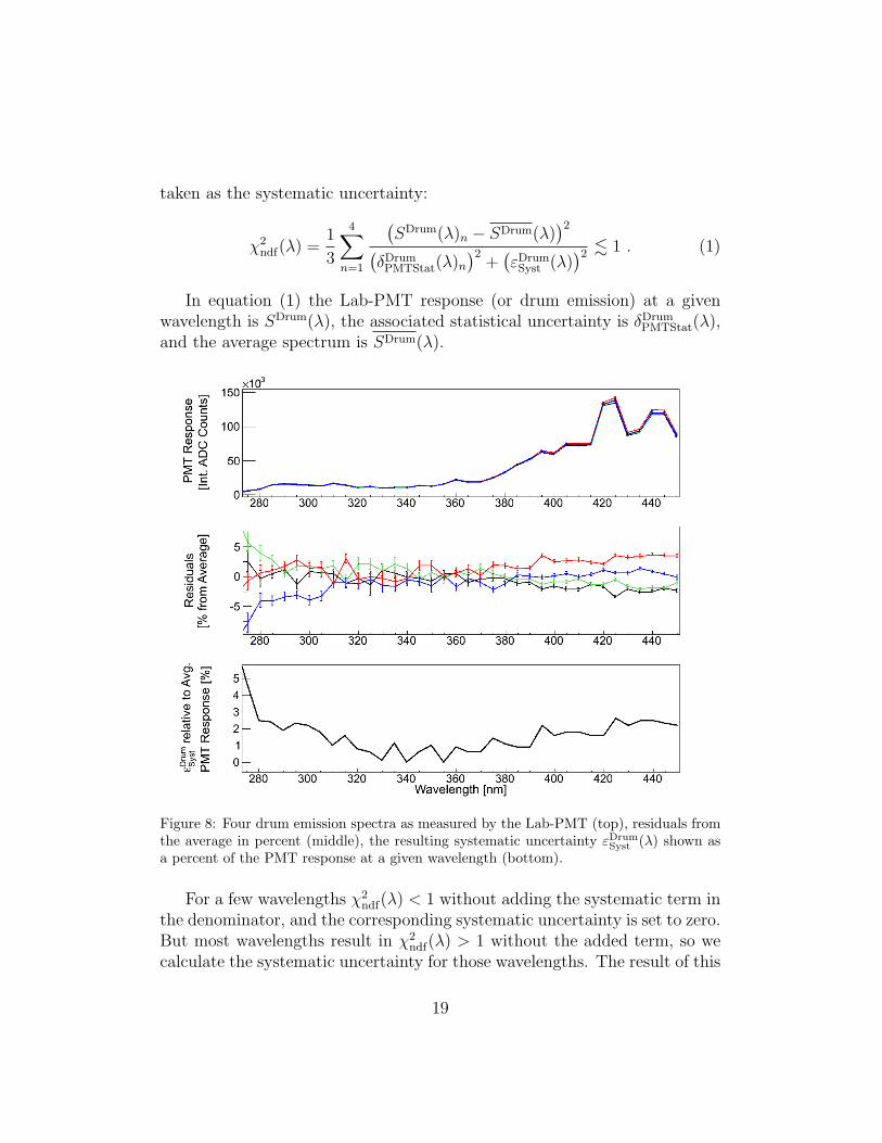
taken as the systematic uncertainty:

χ2ndf(λ) =

1

3

4∑n=1

(SDrum(λ)n − SDrum(λ)

)2(δDrum

PMTStat(λ)n)2

+(εDrum

Syst (λ))2 . 1 . (1)

In equation (1) the Lab-PMT response (or drum emission) at a givenwavelength is SDrum(λ), the associated statistical uncertainty is δDrum

PMTStat(λ),and the average spectrum is SDrum(λ).

Figure 8: Four drum emission spectra as measured by the Lab-PMT (top), residuals fromthe average in percent (middle), the resulting systematic uncertainty εDrum

Syst (λ) shown asa percent of the PMT response at a given wavelength (bottom).

For a few wavelengths χ2ndf(λ) < 1 without adding the systematic term in

the denominator, and the corresponding systematic uncertainty is set to zero.But most wavelengths result in χ2

ndf(λ) > 1 without the added term, so wecalculate the systematic uncertainty for those wavelengths. The result of this

19

procedure is that the non-zero Lab-PMT systematic uncertainties vary fromless than 1% to approximately 3%, and in the important region from 300 nmto 400 nm the average systematic uncertainty is, conservatively, about 1%,see the bottom panel of Figure 8.

As a check, the PD spectra were treated with a similar evaluation of a sys-tematic uncertainty at each wavelength as in equation (1). The correspond-ing systematic uncertainty estimates for the PD would all be approximately1% or smaller. But there is no need to assess a systematic uncertainty on thedrum intensity due to the PD since the PD data are only used to normalizethe PMT data to reduce the spread in PMT measurements, and we use thespread in (normalized) PMT data for the systematic uncertainty.

We estimate the overall systematic uncertainty on the intensity of thedrum at each wavelength based on the QE measurement of the Lab-PMT(δDrum

QESyst(λ) ≈ 1% ) and the four measurements of the drum spectrum(εDrum

Syst (λ) ≈ 1%). Each of these uncertainties is conservatively about 1%in the main region of the FD efficiency and nitrogen fluorescence spectrum,so a reasonable estimate of the overall systematic uncertainty of the drumintensity is found by adding them in quadrature: 1.4%.

5. FD Measurements

During the March 2014 calibration campaign we measured the response ofthe eight telescopes, as specified in Table 1, in steps of 5 nm, over the courseof five days. Data from the monitoring PD were also acquired during the FDmeasurements to be able to control for changes in the drum spectral emission.The procedure for measuring the telescope response to the multi-wavelengthdrum was to first scan from 255 nm to 445 nm in steps of 10 nm, and thenscan from 250 nm to 450 nm in steps of 10 nm. At each wavelength a seriesof 100 pulses from the drum was recorded by the FD data acquisition at arate of 1 Hz. A full telescope response is then an interleaving of these scans.Later in analysis, wavelengths that result in essentially zero FD efficiency -at low and high wavelengths in the scan corresponding to the edges of thenitrogen spectrum - were dropped and set to zero.

In the previous sections we evaluated the systematic uncertainty in thedrum light source intensity as a function of wavelength. The contributionsto this uncertainty are the spread in the four measurements of the drumintensity over the week of the calibration campaign and the systematic un-certainty in the quantum efficiency of the PMT used to measure the drum

20

output.In this section we evaluate the uncertainty in the responses of the tele-

scopes to the drum by comparing the responses of telescopes with the sameoptical components - see Table 1. We do this comparison because we havenot measured every telescope in the observatory, so we have to develop asingle calibration constant for each wavelength for each of the four sets ofoptical components in the table. Then we use these calibration constantsfor all telescopes with like components (again, see Table 1), including thosenot measured. Combining this uncertainty on the FD response, describedbelow, with the drum emission systematic uncertainty will give the overallsystematic uncertainties on the spectral calibration of the telescopes. As wewill see below, of the four combinations of optical components in Table 1three will result in systematics on FD response well below the systematicsfrom the drum emission, but one pair of telescopes will have significantlydifferent responses to the drum resulting in a systematic uncertainty largerthan that from the drum intensity.

5.1. FD Systematic Uncertainties Evaluated by Comparing Similar Telescopes

We assume that the FDs built with like components - the same mirrorand corrector ring types - should give similar responses, and to test thatassumption we make a comparison between them to derive a meaningfulsystematic uncertainty. To that end we perform a χ2 test and introduceparameters to minimize the χ2 such that χ2

ndf . 1 for ndf = 34, wherethere are 35 wavelengths used in the comparison. The parameters introducedare an overall scale factor β that is applied to one of the FD responses,and then εFD which is an estimate of a systematic uncertainty that wouldbe needed to account for the difference between the two telescopes. Thusthe raw response of one of the FDs as a function of wavelength is thenβ ∗

(FDResp(λ) ± δFD

Stat(λ) ± εFD

)in the comparison, where δFD

Stat(λ) is thestatistical uncertainty (small) as mentioned at the end of this section. Thescale factor β does not represent a systematic uncertainty, it just accountsfor any overall difference in response between the two telescopes. This issimilar to performing a relative calibration analysis as in [14] between thetwo telescopes.

The minimization is done in two steps according to equation (2) where

21

the sum is over the Nλ measured wavelength points:

χ2ndf =

1

34

Nλ∑n=1

(FD1(λ)n − β ∗ FD2(λ)n

)2

(δFD1

Stat (λ)n

)2

+(β ∗ δFD2

Stat (λ)n

)2

+(β ∗ εFD

)2 . (2)

First a minimum in χ2 is found by setting εFD = 0 and allowing the scalefactor β to vary. Once β has been determined, εFD is allowed to vary untilχ2

ndf . 1. Prior to the minimization the FD2(λ) response data are normalizedby the ratio of the monitoring PD response as measured at FD1 and FD2 fora given wavelength. This serves to divide out any change in intensity of thelight source as measured by the PD just downstream of the monochromator,and this normalization does, as expected, improve the agreement in responsefor some telescope pairs.

Table 3: εFD and β values obtained via equation (2) for the similarly constructed tele-scopes. The εFD for a given pair of telescopes is given in percentage relative to the averagedresponse of the pair of telescopes at 375 nm.

FDs εFD [%] β

Coihueco 2/3 0.34 0.97Coihueco 4/5 0.48 1.02Los Morados 4/5 0.14 1.01Los Leones 3/4 1.7 1.05

The values for εFD and β are listed in Table 3 for each pair of telescopesthat are constructed with nominally identical components, and the system-atic uncertainties, εFD, are reported as a percentage of the average responseof the two telescopes at 375 nm.

Aside from Los Leones telescopes 3 and 4, the εFD values derived throughthis minimization technique are all less than 0.5 % , and the β scale factorsare all within about 3 % of unity. The values obtained for Los Leones,although larger than the others, are still small. By trying to find a reasonfor this difference we note that telescope 4 was part of the Engineering Array(EA, [15]) together with telescope 5. However, both telescopes were rebuiltafter the EA operation, particularly the mirrors were all replaced by new

22

ones after re-setting the design parameters. So, the discrepancy between LL3 and 4 is highly probably not caused by any difference in used materialsand, in any case, is included in the uncertainties.

We use the εFD calculated for a given pair of FD telescopes as a system-atic uncertainty across all wavelengths for all telescopes of the correspondingconstruction; see Table 1. These systematic uncertainties are then normal-ized by the telescope response at 375 nm and are added in quadrature withthe uncertainties associated with the spread in Lab-PMT measurements ofthe drum (about 1% in important wavelength range, a function of wave-length), and the Lab-PMT QE (1%, not wavelength dependent) to calcu-late the overall systematic uncertainty on telescopes of each combination ofoptical components. An example result is plotted as the red brackets inFigure 9 for the Los Morados telescopes 4 and 5; for this pair (and liketelescopes) the overall systematic uncertainty on the FD response is approx-imately

√12 + 12 + 0.142 = 1.4%, and it is dominated by the uncertainty

in the drum intensity. For the Coihueco instruments the overall systematicuncertainty is about 1.5%. For the telescopes at Los Leones the uncertaintyfrom the difference in response between the two telescopes is larger than thedrum-related systematic uncertainties, and the overall systematic uncertaintyon all of the Los Leones telescopes is about 2.2%.

The statistics of the data taken with the drum light source at the FDtelescopes also contribute to the uncertainties on the calibration constants.The typical spread in the average response of the 440 PMTs to the 100 drumpulses at a given wavelength is 0.4% RMS, which is much smaller than thesystematic uncertainties. Adding the statistical uncertainty in quadraturewith the systematic uncertainties yields the overall uncertainties on the cal-ibration constants listed in Table 4, which are the main result of this work.

5.2. Photodiode Monitor Data

We performed a comparison between the average dark hall PD spectrumand each of the spectra measured for the data-taking nights at the FDs toensure that the light source was stable and was consistent with what hadbeen measured in the lab. An overall correction of 1.00± 0.01 night to nightwas found as the average ratio of the PD response at the FD to that atthe lab to accommodate any overall variations in intensity or response dueto temperature effects, and then we performed a χ2 comparison for all themeasured wavelengths. For all measuring nights at the FDs the PD spectraagree very well, the comparison gives a χ2

ndf ∼ 1 where ndf = 34 for each,

23

Table 4: Overall uncertainties on spectral calibration constants for the pairs of telescopesmeasured and all other (unmeasured) telescopes with the same optical components.

FDs Overall FDs with sameuncertainty [%] components

Coihueco 2/3 1.5 CO2/3Coihueco 4/5 1.5 CO1,4-6, LA, HEATLos Morados 4/5 1.5 LMLos Leones 3/4 2.2 LL1-6

implying that the spectrum as observed by the PD was the same at alllocations.

6. Calculation of the FD Efficiency

We calculate the relative FD efficiency for each telescope by dividing themeasured telescope response to the drum by the measured drum emissionspectrum. The relative drum emission spectrum is measured as described insection 4 and takes into account the Lab-PMT quantum efficiency over therange from 250 nm to 450 nm.

The relative efficiency for a given telescope at a given wavelength, FDReleff (λ),

is calculated for each wavelength from 280 nm to 440 nm in steps of 5 nm:

FDReleff (λ) =

FDResp(λ) ∗QELabPMT(λ)

SDrum(λ)∗ 1

FDeff(λ = 375 nm). (3)

The curves are taken relative to the efficiency of the telescope at 375 nmsince this is what is used in the Pierre Auger Observatory reconstructionsoftware [16] for all FD calculations. The range in wavelength from 280 nmto 440 nm used for evaluating the FD efficiency is smaller than the rangemeasured in the lab because below 280 nm and above 440 nm the light levelis near zero intensity for the nitrogen emission spectrum and the FD responseis also very near zero. As an example, Figure 9 shows the relative efficiencyfor the Los Morados telescopes 4 and 5 based on this work compared withthe previous measurement [9].

The uncertainties in the FD efficiencies have statistical and systematiccomponents associated with the measurement of the relative emission spec-

24

Figure 9: Relative efficiencies for the average of Los Morados telescopes 4 and 5. Top:the five filter curve shown as a dashed blue line [9] and the monochromator result shownas the solid line. Error bars are statistical uncertainties, and the red brackets are thesystematic uncertainties calculated as described in section 5. Bottom: difference betweenthe five filter result and this work. The error bars and brackets are the same as in the topplot, shown here for clarity.

trum of the drum, the Lab-PMT QE, and the FD response to the multi-wavelength drum. The statistical uncertainties associated with the lab workand the FD responses are propagated through the calculation of the FDefficiency via equation (3) as a function of wavelength. All systematic uncer-tainties described above associated with the lab work, the Lab-PMT and itsQE, the FD response, and εFD for a given FD telescope, are added togetherin quadrature as a function of wavelength.

For much of the wavelength range the new results agree with the olderfive-point scan. The disagreement at the shortest and longest wavelengths is

25

perhaps not surprising since the previous lowest and highest measurementswere at 320 nm and 405 nm, and the efficiency was extrapolated to zero fromthose points following the piecewise curve [11]. The efficiency was assumedto go to zero below 295 nm and above 425 nm.

7. Comparison of telescopes with differing optical components

After estimating the systematic uncertainties for each measured FD tele-scope, εFD, we made a χ2 comparison between the six combinations of unlikeFD optical components listed in Table 1 to determine whether the unlike com-ponents result in any different telescope responses. In calculating the χ2

ndf

for the differently constructed FD telescopes we use the ratio of the PD datataken at the corresponding FDs to normalize the average response of one ofthe FD types. The PD data from the two FD data-taking nights are averagedas a function of wavelength and the ratio of the PD averages from the twotypes of FDs are applied to the combined FD response along with the statis-tical and systematic uncertainties. Using this normalization serves to divideout any differences in the drum spectrum between the two measurements ofthe FD types. An example for calculating the χ2 between the average ofCoihueco 2 and Coihueco 3 (SCO23(λ)n) and the average of Coihueco 4 and5 follows. The uncertainties in equation 4 have obvious labels; for exampleεCO23

FD is the systematic uncertainty for the Coihueco telescopes 2 and 3 fromTable 3.

χ2ndf =

1

34

Nλ∑n=1

(SCO23(λ)n − PDRatio(λ)n ∗ SCO45(λ)n

)2

(δCO23

Stat (λ)n

)2+(PDRatio(λ)n ∗ δCO45

Stat (λ)n

)2+(εCO23

FD

)2+(εCO45

FD

)2 ,

PDRatio(λ) ≡ SPDCO23(λ)

SPDCO45(λ)

.

(4)

The results of the comparisons are shown in Table 5. The telescopes withdifferent components are all significantly different from each other exceptwhen comparing the average of Los Leones telescopes 3 and 4 to the averageof Los Morados telescopes 4 and 5. In principle this low χ2 could indicate thatall telescopes constructed with components like those at Los Leones 3 and

26

4 and those constructed like Los Morados telescopes 4 and 5 have the sameresponse, and therefore could share the relative calibration constants thatare the goal of this work. However, the two detectors at Los Leones have amuch greater difference in response between them than do the two telescopesfrom Los Morados: the systematic uncertainty in Table 3 for Los Leonestelescopes is more than a factor of 10 larger than that for Los Morados ones.The large systematic uncertainty for the telescopes at Los Leones could bemasking a real difference with those at Los Morados. For this reason we feelit is reasonable not to combine the Los Leones and Los Morados telescopesto calculate the final spectral calibration constants.

We conclude that all four sets of FD telescopes listed in Table 1 needdifferent spectral calibrations, and four sets of calibration constants havebeen computed.

Examining the results in Table 5 and Table 1 we note that the largest χ2ndf

values in Table 5 are associated with changing mirrors not changing correctorrings. For example, comparing Coihueco 4/5 with Los Morados 4/5 changesonly the mirror and gives a χ2

ndf of 55, but comparing Coihueco 4/5 withCoihueco 2/3, which changes only the corrector ring, yields a χ2

ndf of 5.6.Changing both components by comparing Coihueco 2/3 with Los Morados4/5 gives a χ2

ndf of 161, but we note that the telescopes at Los Morados havea very small systematic uncertainty in Table 3. These examples have so farleft out the Los Leones telescopes. The large systematic uncertainty derivedby comparing the two Los Leones telescopes reduces the χ2

ndf values whencomparing to other telescopes, but the idea that the mirrors are the maineffect is still present when comparing the Los Leones telescopes to the others.

Table 5: Comparison of spectral response for FD telescopes with different components.χ2ndf values obtained for the sets in Table 1, where ndf = 34.

Comparison χ2ndf

Coihueco 2/3 vs. Coihueco 4/5 2.4Los Morados 4/5 vs. Los Leones 3/4 0.21Coihueco 4/5 vs Los Morados 4/5 57Coihueco 2/3 vs. Los Leones 3/4 10Coihueco 2/3 vs. Los Morados 4/5 144Los Leones 3/4 vs. Coihueco 4/5 6.7

27

8. Effect on Physics Measurables

To evaluate the effect a new calibration has on physics measurables, wereconstructed a set of events using the new calibration and compare to re-sults from that same set of events using the prior calibration. When wedid this exercise upon changing from initial piecewise to the five-point cali-bration, the reconstructed energies increased about 4% at 1018 eV, and theincrease lessened slightly to 3.6% at 1019 eV [12]. The lessening of the en-ergy increase due the five-point calibration is understood because much of thechange in calibration was at low wavelengths, and the five-point calibrationmakes the FDs less efficient at short wavelengths making the reconstructedenergy higher. The higher energy events make more light, and they can bedetected at greater distances than lower energy events. But at greater dis-tances more of the short wavelength light will be Rayleigh scattered away,so the lower wavelengths - and the change in calibration there - do not affectthe higher energy events as much when we change to the new calibration.

When we change from the five-point to the calibration described here, thereconstructed energies increase on average over all FD telescopes by about1%, and that increase is relatively flat in energy. However, this increase isnot the same at all the telescopes. The increase in reconstructed energy isgreatest at Los Leones, about 2.8% at 1018 eV falling to 2.5% at 1019 eV. ForLos Morados the reconstructed event energies increase by about 1.8% withoutmuch energy dependence. For all other telescopes the energy increases, butthose increases are less than 0.35% for all energies.

All these changes in the reconstructed energy are important to knowto fully characterize the telescopes. Regarding the associated uncertainties,they are all significantly smaller than the uncertainties involved in the energyscale for the FD telescopes (see Table 3 in [1]), particularly the 3.6% fromthe Fluorescence yield and the 9.9% from the FD calibration.

9. Conclusions

Determining the spectral response of the Pierre Auger Observatory fluo-rescence telescopes is essential to the success of the experiment. A method us-ing a monochromator-based portable light source has been used for eight FDtelescopes with measurements performed every five nanometers from 280 nmto 440 nm. With the calibration of these eight telescopes, the four possiblecombinations of different optical components in the FD were covered, thusassuring the spectral calibration of all FD telescopes at the observatory.

28

The uncertainty associated with the emission spectrum of the drum lightsource used for the calibration was found to be 1.4%, which is an improvementon our previous 3.5% [9].

For the present work we compared telescopes with nominally the sameoptical components, and we find that such pairs have the same spectral re-sponse within a fraction of a percent - as expected - for three out of thefour pairs of like telescopes. But one pair with like components, the old-est telescopes in the observatory, shows a significant difference in spectralresponse.

The overall uncertainty in the FD spectral response is 1.5% for 21 ofthe 27 telescopes. The overall systematic uncertainty for the remaining sixtelescopes is 2.2%, and is somewhat larger on account of the larger differencebetween the two telescopes measured.

We also compared the differently constructed telescopes. These compar-isons show significantly different efficiencies as a function of wavelength, withdifferences mainly in the rising edge of the efficiency curve between 300 nmand 340 nm. The differences seem to come mostly from the two different mir-ror types, and they are reflected in different calibration constants for each ofthe four combinations of optical components.

The new calibration constants affect the reconstruction of EAS events,and we looked at two important quantities. The primary cosmic ray energyincreases by 1.8% to 2.8% for half of the telescopes in the observatory, andfor the other half the change in energy is negligible. The position of themaximum in shower development in the atmosphere, Xmax, is not changedsignificantly by the change in calibration.

Acknowledgments

The successful installation, commissioning, and operation of the PierreAuger Observatory would not have been possible without the strong com-mitment and effort from the technical and administrative staff in Malargue.We are very grateful to the following agencies and organizations for financialsupport:

Argentina – Comision Nacional de Energıa Atomica; Agencia Nacionalde Promocion Cientıfica y Tecnologica (ANPCyT); Consejo Nacional de In-vestigaciones Cientıficas y Tecnicas (CONICET); Gobierno de la Provin-cia de Mendoza; Municipalidad de Malargue; NDM Holdings and ValleLas Lenas; in gratitude for their continuing cooperation over land access;

29

Australia – the Australian Research Council; Brazil – Conselho Nacionalde Desenvolvimento Cientıfico e Tecnologico (CNPq); Financiadora de Es-tudos e Projetos (FINEP); Fundacao de Amparo a Pesquisa do Estadode Rio de Janeiro (FAPERJ); Sao Paulo Research Foundation (FAPESP)Grants No. 2010/07359-6 and No. 1999/05404-3; Ministerio de Ciencia eTecnologia (MCT); Czech Republic – Grant No. MSMT CR LG15014,LO1305, LM2015038 and CZ.02.1.01/0.0/0.0/16 013/0001402; France –Centre de Calcul IN2P3/CNRS; Centre National de la Recherche Sci-entifique (CNRS); Conseil Regional Ile-de-France; Departement PhysiqueNucleaire et Corpusculaire (PNC-IN2P3/CNRS); Departement Sciences del’Univers (SDU-INSU/CNRS); Institut Lagrange de Paris (ILP) Grant No.LABEX ANR-10-LABX-63 within the Investissements d’Avenir ProgrammeGrant No. ANR-11-IDEX-0004-02; Germany – Bundesministerium fur Bil-dung und Forschung (BMBF); Deutsche Forschungsgemeinschaft (DFG);Finanzministerium Baden-Wurttemberg; Helmholtz Alliance for Astropar-ticle Physics (HAP); Helmholtz-Gemeinschaft Deutscher Forschungszen-tren (HGF); Ministerium fur Innovation, Wissenschaft und Forschungdes Landes Nordrhein-Westfalen; Ministerium fur Wissenschaft, Forschungund Kunst des Landes Baden-Wurttemberg; Italy – Istituto Nazionale diFisica Nucleare (INFN); Istituto Nazionale di Astrofisica (INAF); Min-istero dell’Istruzione, dell’Universita e della Ricerca (MIUR); CETEMPSCenter of Excellence; Ministero degli Affari Esteri (MAE); Mexico – Con-sejo Nacional de Ciencia y Tecnologıa (CONACYT) No. 167733; Univer-sidad Nacional Autonoma de Mexico (UNAM); PAPIIT DGAPA-UNAM;The Netherlands – Ministerie van Onderwijs, Cultuur en Wetenschap; Ned-erlandse Organisatie voor Wetenschappelijk Onderzoek (NWO); Stichtingvoor Fundamenteel Onderzoek der Materie (FOM); Poland – National Cen-tre for Research and Development, Grants No. ERA-NET-ASPERA/01/11and No. ERA-NET-ASPERA/02/11; National Science Centre, Grants No.2013/08/M/ST9/00322, No. 2013/08/M/ST9/00728 and No. HARMONIA5–2013/10/M/ST9/00062, UMO-2016/22/M/ST9/00198; Portugal – Por-tuguese national funds and FEDER funds within Programa OperacionalFactores de Competitividade through Fundacao para a Ciencia e a Tec-nologia (COMPETE); Romania – Romanian Authority for Scientific Re-search ANCS; CNDI-UEFISCDI partnership projects Grants No. 20/2012and No.194/2012 and PN 16 42 01 02; Slovenia – Slovenian ResearchAgency; Spain – Comunidad de Madrid; Fondo Europeo de Desarrollo Re-gional (FEDER) funds; Ministerio de Economıa y Competitividad; Xunta

30

de Galicia; European Community 7th Framework Program Grant No. FP7-PEOPLE-2012-IEF-328826; USA – Department of Energy, Contracts No.DE-AC02-07CH11359, No. DE-FR02-04ER41300, No. DE-FG02-99ER41107and No. de-sc0011689; National Science Foundation, Grant No. 0450696;The Grainger Foundation; Marie Curie-IRSES/EPLANET; European Parti-cle Physics Latin American Network; European Union 7th Framework Pro-gram, Grant No. PIRSES-2009-GA-246806; European Union’s Horizon 2020research and innovation programme (Grant No. 646623); and UNESCO.

References

[1] A. Aab, et al., The Pierre Auger Cosmic Ray Observatory, NuclearInstruments and Methods in Physics Research Section A: Accelerators,Spectrometers, Detectors and Associated Equipment 798 (2015) 172–213.

[2] I. Allekotte, et al., The Surface Detector System of the Pierre Auger Ob-servatory, Nuclear Instruments and Methods in Physics Research SectionA: Accelerators, Spectrometers, Detectors and Associated Equipment586 (3) (2008) 409–420. doi:10.1016/j.nima.2007.12.016.

[3] J. Abraham, et al., The Fluorescence Detector of the Pierre Auger Ob-servatory, Nuclear Instruments and Methods in Physics Research SectionA: Accelerators, Spectrometers, Detectors and Associated Equipment620 (2-3) (2010) 227–251. doi:10.1016/j.nima.2010.04.023.

[4] T. H.-J. Mathes, et al., The HEAT Telescopes of the Pierre Auger Ob-servatory Status and First Data, Proc. of the 32nd ICRC, Beijing, China,2011, pp. 153–156.

[5] M. Roth, et al., Measurement of the UHECR energy spectrum usingdata from the Surface Detector of the Pierre Auger Observatory, Proc.of the 30th ICRC, Merida, Mexico, 2007.

31

[6] J. Abraham, et al., Observation of the Suppression of the Flux of CosmicRays above 4×1019 eV, Physical Review Letters 101 (2008) 061101. doi:10.1103/PhysRevLett.101.061101.

[7] J. Brack, et al., Absolute Calibration of a Large-diameter Light Source,JINST 8 (2013) P05014. arXiv:1305.1329, doi:10.1088/1748-0221.

[8] R. Knapik, et al., The Absolute, Relative and Multi-wavelength Cali-bration of the Pierre Auger Observatory Fluorescence Detectors, Proc.of the 30th ICRC, Merida, Mexico, 2007.

[9] A. Rovero, P. Bauleo, J. Brack, J. Harton, R. Knapik, Multi-wavelengthCalibration Procedure for the Pierre Auger Observatory FluorescenceDetectors, Astroparticle Physics 31 (4) (2009) 305–311. doi:10.1016/

j.astropartphys.2009.02.009.

[10] M. Ave, et al., Spectrally Resolved Pressure Dependence Measurementsof Air Fluorescence Emission with AIRFLY, Nuclear Instruments andMethods in Physics Research Section A: Accelerators, Spectrometers,Detectors and Associated Equipment 597 (1) (2008) 41–45.

[11] J. A. Matthews, Optical Calibration of the Auger Fluorescence Tele-scopes, in: Astronomical Telescopes and Instrumentation, InternationalSociety for Optics and Photonics, 2003, pp. 121–130.

[12] A. Aab, et al., The Pierre Auger Observatory: Contributions to the 33rd

International Cosmic Ray Conference (ICRC 2013) arXiv:1307.5059.

[13] J. Brack, R. Meyhandan, G. Hofman, J. Matthews, Absolute Photomet-ric Calibration of Large Aperture Optical Systems, Astroparticle Physics20 (6) (2004) 653–659.

[14] C. Aramo, et al., Optical Relative Calibration and Stability Monitoringfor the Auger Fluorescence Detector, Proc. of the 29th ICRC, Pune,India, 2005.

[15] J. Abraham, et al., Properties and performance of the prototype in-strument for the Pierre Auger Observatory, Nuclear Instruments andMethods in Physics Research A 523 (2004) 50–95. doi:10.1016/j.

nima.2003.12.012.

32

[16] S. Argiro, et al., The Offline Software Framework of the Pierre AugerObservatory, Nuclear Instruments and Methods in Physics Research Sec-tion A: Accelerators, Spectrometers, Detectors and Associated Equip-ment 580 (3) (2007) 1485–1496.

33