Spectral Analysis Using a Deep-MemoryOscilloscope Fast Fourier Transform (FFT)For Use with Infiniium 54830B Series Deep-Memory Oscilloscopes

Application Note 1383-1

Introduction

Many of today’s digital oscillo-scopes include a Fast FourierTransform (FFT) for frequency-domain analysis. This feature isespecially valuable for oscillo-scope users who have limited orno access to a spectrum analyzeryet occasionally need frequency-domain analysis capability. Anintegrated oscilloscope FFT pro-vides a cost effective, space sav-ing alternative to a dedicatedspectrum analyzer. Though thelatter does exhibit better dynamicrange and less distortion, the dig-ital oscilloscope offers severalcompelling benefits.1

The Agilent TechnologiesInfiniium 54800 Series digitaloscilloscopes include FFT func-tions for computing both magni-tude and phase. Several usefulfeatures assist in spectral analy-sis. Controls adjust memorydepth, sampling rate, verticalscale and horizontal scale of theFFT. Automatic measurementsand markers measure spectralpeak frequencies and magnitudesas well as deltas between peaks.The Infiniium Help system pro-vides extensive information on

FFT theory and application.Several features designed prima-rily for time-domain analysis arealso useful for the FFT. Displaytraces can be annotated andsaved to a file. The oscilloscopeconfiguration can be saved andrecalled as a setup file. Func-tions can be chained together toperform complex tasks, such ascomputing the average, maxi-mum or minimum of several FFTspectrums. Measurement statis-tics are available for computingthe mean and standard deviationof a measurement over severalacquisitions. With all this capa-bility, the oscilloscope FFT pro-vides a very convenient tool forspectral analysis.

The deep-memory Infiniium54830B family of oscilloscopesenable an increase in the recordlength of the FFT, which in turnimproves the frequency spec-trum estimate. Longer recordlengths provide finer frequencyresolution and better dynamicrange. By upgrading the proces-sor speed and improving the effi-ciency of the FFT algorithm, theInfiniium deep-memory oscillo-scopes can perform FFTs on longrecords very quickly.

Table of Contents

Introduction . . . . . . . . . . . . . . . . . . . . . . . . 1

FFT Fundamentals . . . . . . . . . . . . . . . . . . 2Discrete Fourier Transform . . . . . . . . 2Sampling Effects . . . . . . . . . . . . . . . . . 4Spectral Leakage and Windowing . . 6

Practical Considerations . . . . . . . . . . . . 8Frequency Span and Resolution . . . . 8Dynamic Range . . . . . . . . . . . . . . . . . 10Averaging . . . . . . . . . . . . . . . . . . . . . . 13Window Selection. . . . . . . . . . . . . . . 15Equivalent Time Sampling . . . . . . . . 16

Application . . . . . . . . . . . . . . . . . . . . . . . 17Characterizing an AM Signal. . . . . . 17Selecting Sampling Rate andMemory Depth. . . . . . . . . . . . . . . . . . 18Scaling Time and Frequency . . . . . . 18Resulting FFT Spectrum . . . . . . . . . . 19

Support, Services, and Assistance . . . . . . . . . . . . . . . . . . . . 20

2

This application note begins with a discussion of FFT funda-mentals and highlights thosecharacteristics that are importantfor understanding FFT-basedspectral analysis. It goes on toexplain practical considerationsfor using an oscilloscope FFT for spectral analysis and techniques that can be used toimprove dynamic range and accuracy. Finally, it concludeswith a specific application thatillustrates the benefits of a deep-memory oscilloscope FFT formaking high-frequency resolutionspectral measurements.

Discrete Fourier Transform

To better understand the limita-tions of using an oscilloscope FFTfor spectral analysis, it is impor-tant to understand some funda-mental properties of the DiscreteFourier Transform (DFT) and theeffects of sampling. A brief reviewis covered here. The reader isreferred to other sources formore detailed information.

The DFT represents discrete samples of the continuous

Fourier transform of a finitelength sequence.2 The DFT for asequence, x(nT), is given by:3

Equation 1

whereN = number of samplesF = spacing of frequency

domain samplesT = sample period in the

time domain

The FFT is simply an efficientalgorithm for computing the DFT.Actually, there are several FFTalgorithms. Infiniium uses aradix-2 FFT algorithm for com-puting the DFT. A radix-2 FFT iscomputed on a number of pointsequal to a power of 2. The effi-ciency of the FFT is oftenexpressed in terms of the numberof complex multiplications. Thenumber of complex multiplica-tions for a radix-2 FFT can beshown to be Nlog2N. This is a bigimprovement over the number ofcomputations for a DFT, which isapproximately N2. For example,for a one-million-point sequence,the FFT takes 0.002% of the DFTcomputation time.2

The spacing of the frequency-domain samples or bins in theDFT is given by the followingequation:

Equation 2

whereFs = sampling frequency

Thus, the frequency resolutioncan be improved by increasing Nor decreasing Fs.

The DFT is symmetrical aboutN/2. The magnitude of the DFT isan even symmetric function andthe phase is an odd symmetricfunction. Infiniium plots only thefirst half of the FFT points sinceno additional information is pro-vided by the remaining points.The frequency of a particular FFTpoint, k, is:

Equation 3

The maximum frequency plottedis Fs/2, where k = N/2.

FFT Fundamentals

X(kF) = ∑ x(nT)e-j2πkFntN-1

n = 0 F = = 1

NTFsN

Fk = kFsN

Discrete Fourier Transform continued

The DFT is a complex exponentialfrom which both magnitude andphase can be computed. Infiniiumhas functions for computing boththe magnitude and phase. Thephase is computed in degrees.The magnitude is computed indBm.3 The voltage form for dBm is:

Equation 4

where

The reference voltage, VREF, isdefined as the voltage that pro-duces 1 milliwatt of power into50 Ω. For example, if 1 volt dc isconnected to Infiniium, then themagnitude of the FFT result at0 Hz frequency will be approxi-mately 13 dBm:

3

FFT Fundamentals

P(dBm) = 20log(VRMS / VREF)

VREF =

√0.001 watts * 50 Ω = 0.2236 volts

20log(1.0 / 0.2236) = 13.0 dBm

The Infiniium waveform recordlength captured is generally not apower of 2. However, the radix-2FFT requires a number of pointsequal to a power of 2. Infiniiumhandles this by padding the endof the waveform with zeros to get to the next power of 2sequence length.

Although zero padding increasesthe number of points, it does notchange the shape of X(F). It sim-ply extends the number of pointsin the DFT. For example, if zeropadding extends the sequencelength by a factor of 2, then everyother point of the DFT of thezero-padded sequence has thesame value as the DFT of theunpadded sequence. Thus, zeropadding has the same effect asinterpolation: it fills in pointsbetween frequency samples, giv-ing a better visual image of thecontinuous Fourier transform.

4

FFT Fundamentals

Sampling Effects

The Fourier transform of an ana-log signal, xa(t), is defined by:2

Equation 5

To obtain a digital representa-tion, x(n), of an analog signal,xa(t), a digital oscilloscope samples the signal at uniformintervals, T:

Equation 6

Equation 6 assumes the samplingprocess is ideal such that there isno voltage quantization or otherdistortion. The Fourier transformof this ideal discrete timesequence is:2

Equation 7

Equation 7 shows the relation-ship between the Fourier trans-form, Xa(F), of the continuous signal, and the Fourier transform,X(F), of the discrete timesequence. X(F) is the sum of aninfinite number of amplitude-scaled, frequency-scaled, andtranslated versions of Xa(F).

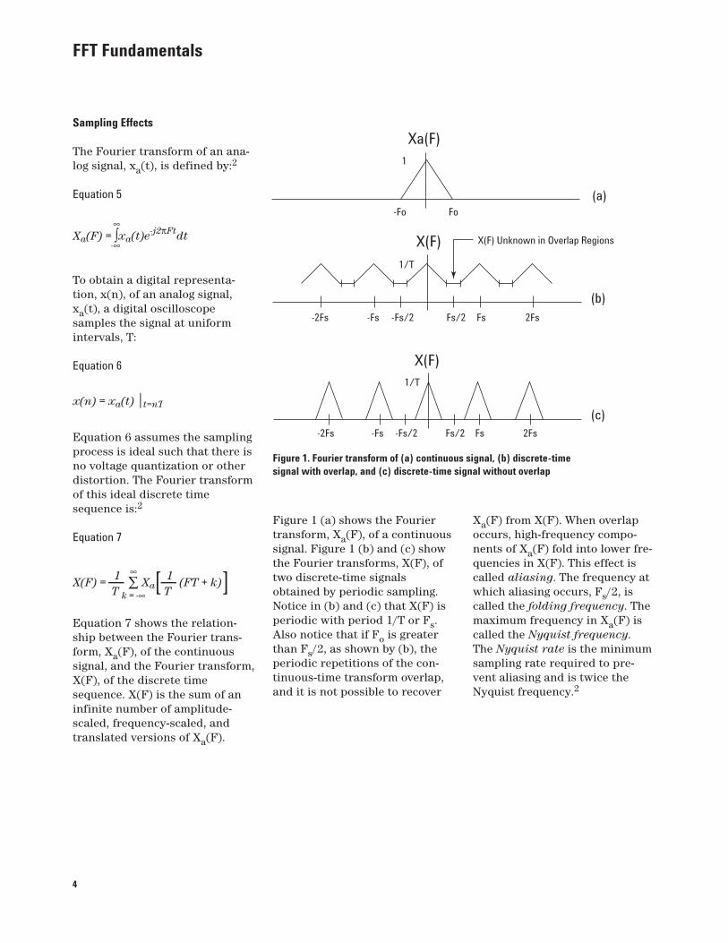
Figure 1 (a) shows the Fouriertransform, Xa(F), of a continuoussignal. Figure 1 (b) and (c) showthe Fourier transforms, X(F), oftwo discrete-time signalsobtained by periodic sampling.Notice in (b) and (c) that X(F) isperiodic with period 1/T or Fs.Also notice that if Fo is greaterthan Fs/2, as shown by (b), theperiodic repetitions of the con-tinuous-time transform overlap,and it is not possible to recover

Xa(F) from X(F). When overlapoccurs, high-frequency compo-nents of Xa(F) fold into lower fre-quencies in X(F). This effect iscalled aliasing. The frequency atwhich aliasing occurs, Fs/2, iscalled the folding frequency. Themaximum frequency in Xa(F) iscalled the Nyquist frequency. The Nyquist rate is the minimumsampling rate required to pre-vent aliasing and is twice theNyquist frequency.2

Xa(F)1

(a)

(b)

(c)

-2Fs

Fo

X(F)

X(F)

-Fs -Fs/2 2FsFsFs/2

-Fo

-2Fs -Fs -Fs/2 2FsFsFs/2

1/T

1/T

X(F) Unknown in Overlap Regions

Figure 1. Fourier transform of (a) continuous signal, (b) discrete-timesignal with overlap, and (c) discrete-time signal without overlap

Xa(F) = ∫xa(t)e-j2πFtdt∞

-∞

x(n) = xa(t) |t=nT

X(F) = ∑ Xa[ (FT + k)]∞

k = -∞

1T

1T

5

Equation 8 can be used to com-pute the alias frequency, F', fromthe original frequency, F:

Equation 8

Sampling Effects continued

It is insightful to consider aliasingfrom a time-domain perspective.Assume a sine wave signal is sam-pled uniformly. If there are lessthan two samples per period,then it is not possible to deter-mine the frequency of the contin-uous sine wave signal from thesampled version. In this case, thesampled version will appear to bea sine wave at a lower frequency.

If the sampling rate is at leasttwice the highest frequency con-tent in the analog signal, no alias-ing will occur, and the DFT of thesampled sequence will provide agood estimate of the Fouriertransform of the analog signal.

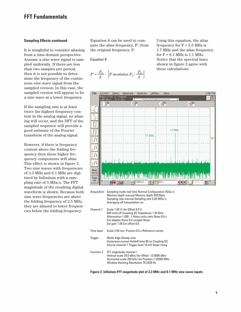
However, if there is frequencycontent above the folding fre-quency then these higher fre-quency components will alias.This effect is shown in figure 2.Two sine waves with frequenciesof 3.3 MHz and 6.1 MHz are digi-tized by Infiniium with a sam-pling rate of 5 MSa/s. The FFTmagnitude of the resulting digitalwaveform is shown. Because bothsine wave frequencies are abovethe folding frequency of 2.5 MHz,they are aliased to lower frequen-cies below the folding frequency.

Figure 2. Infiniium FFT magnitude plot of 3.3 MHz and 6.1 MHz sine wave inputs

FFT Fundamentals

Using this equation, the alias frequency for F = 3.3 MHz is1.7 MHz and the alias frequencyfor F = 6.1 MHz is 1.1 MHz. Notice that the spectral linesshown in figure 2 agree withthese calculations.

F' = - |F modulus Fs - |Fs2

Fs2

Acquisition Sampling mode real time Normal Configuration 4GSa/sMemory depth manual Memory depth 65536ptsSampling rate manual Sampling rate 5.00 MSa/sAveraging off Interpolation on

Channel 1 Scale 1.00 V/div Offset 0.0 VBW limit off Coupling DC Impedance 1 M OhmAttenuation 1.000 : 1 Atten units ratio Skew 0.0 sExt adapter None Ext coupler NoneExt gain 1.00 Ext offset 0.0

Time base Scale 2.00 ms/ Postion 0.0 s Reference center

Trigger Mode edge Sweep autoHysteresis normal Holdoff time 80 ns Coupling DCSource channel 1 Trigger level 10 mV Slope rising

Function 2 FFT magnitude channel 1Vertical scale 20.0 dBm/div Offset -13.0000 dBmHorizontal scale 250 kHz/div Position 1.25000 MHzWindow Hanning Resolution 76.2939 Hz

6

1.2

1

0.8

-0.2

0

0.2

0.4

0.6

-0.5 -0.4 -0.3 -0.2 -0.1 0 0.1 0.2 0.3 0.4 0.5

TIME (x=t/T)

w(x

)/w

(0)

Rectangular, Hanning And Flottop Window Functions

RectangularHanningFlattop

Figure 3. Infiniium FFT window functions (top) and corresponding frequencyspectrums (bottom)

Spectral Leakage and Windowing

The DFT is computed on a finitelength sequence. It attempts toapproximate the ContinuousFourier Transform (CFT), whichintegrates over all time. The DFTis a sampled version of the CFT ofan infinite sequence formed byreplicating the finite sequence aninfinite number of times.

If the end points of the finitesequence do not match, then theinfinite sequence will have a dis-continuity between adjacent peri-ods of the finite sequence. Thisdiscontinuity in the time domaincauses spectral leakage in thefrequency domain. In general,when a digital oscilloscope cap-tures a signal it does not capturean integral number of periods,which introduces a discontinuityin the periodically extended sig-nal. Thus, the FFT computed bythe digital oscilloscope almostalways shows spectral leakage.The spectral leakage causes thefine spectral lines to spread outinto wider lobes.

Another way to explain spectralleakage is to consider the finitesequence as a product of two infi-nite length sequences: the origi-nal sequence and a windowsequence. The window sequenceis nonzero for a finite number ofsamples and zero elsewhere. Bymultiplying the infinite sequenceby the window sequence, the win-dow extracts a finite chunk of theinfinite sequence. Multiplicationin the time domain correspondsto convolution in the frequencydomain. So the resulting Fouriertransform of the finite lengthsequence is just the Fourier transform of the infinite sequenceconvolved with the Fourier trans-form of the window sequence.

FFT Fundamentals

0

-20

-40

-60

-180

-160

-140

-120

-100

-80

-200-0.5 0.50.40.30.20.10-0.1-0.2-0.3-0.4

Frequency Spectrum For Rectangular, Hanning And Flattop Windows

FREQ (HZ)

MA

GN

ITU

DE

(dB

)

N = 1000 pts, fs = 20 HzRectangularHanningFlattop

7

Spectral Leakage and Windowingcontinued

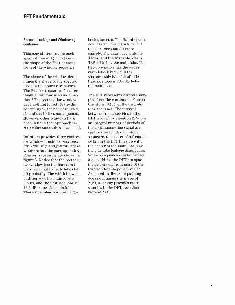
This convolution causes eachspectral line in X(F) to take onthe shape of the Fourier trans-form of the window sequence.

The shape of the window deter-mines the shape of the spectrallobes in the Fourier transform.The Fourier transform for a rec-tangular window is a sinc func-tion.2 The rectangular windowdoes nothing to reduce the dis-continuity in the periodic exten-sion of the finite time sequence.However, other windows havebeen defined that approach thezero value smoothly on each end.

Infiniium provides three choicesfor window functions, rectangu-lar, Hanning, and flattop. Thesewindows and the correspondingFourier transforms are shown infigure 3. Notice that the rectangu-lar window has the narrowestmain lobe, but the side lobes falloff gradually. The width betweenboth zeros of the main lobe is2 bins, and the first side lobe is13.3 dB below the main lobe.These side lobes obscure neigh-

boring spectra. The Hanning win-dow has a wider main lobe, butthe side lobes fall off moresharply. The main lobe width is4 bins, and the first side lobe is31.5 dB below the main lobe. Theflattop window has the widestmain lobe, 8 bins, and thesharpest side lobe fall off. Thefirst side lobe is 70.4 dB belowthe main lobe.

The DFT represents discrete sam-ples from the continuous Fouriertransform, X(F), of the discrete-time sequence. The intervalbetween frequency bins in theDFT is given by equation 2. Whenan integral number of periods ofthe continuous-time signal arecaptured in the discrete-timesequence, the center of a frequen-cy bin in the DFT lines up withthe center of the main lobe, andthe side lobe leakage disappears.When a sequence is extended byzero padding, the DFT bin spac-ing gets smaller and more of thetrue window shape is revealed.As stated earlier, zero paddingdoes not change the shape ofX(F), it simply provides moresamples in the DFT, revealingmore of X(F).

FFT Fundamentals

8

Frequency Span and Resolution

The previous sections describedseveral properties and character-istics of the FFT and samplingthat effect the accuracy of the fre-quency spectral estimate. Thissection focuses on the practicalaspects of using an Infiniiumdeep-memory oscilloscope forspectral analysis. The benefits ofdeep memory on FFT resolutionand dynamic range are describedin detail. Several characteristicsof the oscilloscope effect thedynamic range. These factors andusing averaging to improve thedynamic range are described, aswell as methods for selecting theproper window function for par-ticular types of analysis. Also,this section explains how to con-figure the oscilloscope timerange, sampling rate and memorydepth to get the desired FFT fre-quency span, resolution andupdate rate.

The maximum sampling rate currently available from theInfiniium deep-memory oscillo-scopes is 4 GSa/s, which allowsfor FFT-based spectral analysisup to 2 GHz. The maximum mem-ory depth currently available is16 MSa. When the full samplingrate and memory depth areemployed, Infiniium can providea frequency span of 2 GHz with afrequency resolution of 250 Hz.

It is important to realize thatInfiniium computes the FFT forthose time-domain samples thatfall onscreen only. Offscreen

samples are ignored. To get all thetime-domain samples onscreenfor a manual sampling rate set-ting, the user simply adjusts thehorizontal scale for a longer time range.

Both sampling rate and memorydepth can be controlled manually.In automatic mode, the memorydepth is adjusted to get the maxi-mum sampling rate possible forthe current time range. Althoughthis is a convenient feature fortime-domain analysis, it is notalways what the user wants forfrequency-domain analysis. Inmany cases, the user will pur-posely reduce the sampling rateto improve the frequency resolu-tion. The user may also reducethe memory depth to improve theFFT update rate.

The frequency resolution of theFFT depends on both the sam-pling rate and the number ofpoints, as shown by equation 2.The resolution can be improvedby either increasing the numberof points or decreasing the sam-pling rate. However, decreasingthe sampling rate reduces themaximum frequency computedand opens the door to additionalaliasing. The FFT frequency reso-lution can be easily determinedfrom the time range setting of theoscilloscope, as shown by the following equation:

Equation 9

From the information presentedearlier, it is now possible to deter-mine the frequency resolutionand span of the Infiniium FFT fora particular sampling rate andrecord length.

For example, assume the sam-pling rate is set to 4 GSa/s andthe memory depth is set to100,000 points. In this case,Infiniium will zero-pad the num-ber of points to the next power of2 or 131,072 points. The frequen-cy span displayed will cover halfthe sampling frequency or 2 GHz.The frequency resolution will be4 GSa/s divided by 131,072 or30.5176 kHz. Since the FFT iscomputed only for those pointsthat fall onscreen, to get all thepoints onscreen, the horizontalscale must be set to 2.5 µs/div orslower. The horizontal scale set-ting required to get all the dataonscreen for a particular sam-pling rate and memory depth isshown by the following equation:

Equation 10

Generally, it is not necessary toapply this equation in practice.The user simply adjusts the timerange until all the data isonscreen. The memory bar dis-played at the top of the screensimplifies this adjustment.

Practical Considerations

F = = 1

NT1

Time Range

Horizontal Scale ≥ s / divN

10Fs

9

Figure 4. Infiniium FFT spectrum showing the impact of deep memory onimproved FFT resolution

Practical Considerations

Frequency Span and Resolution continued

Figure 4 shows the impact ofdeep memory on the resolution ofthe FFT spectrum. The spectrumshown is produced from a signalcontaining two sine waves ofnearly identical frequencies, F1and F2. F1 is 75.000273 MHz andF2 is 75.001546 MHz. The fre-quency delta between F1 and F2is 1.273 kHz.

The sampling rate is set at200 MSa/s, which is more than theNyquist rate of 150.003092 MHz.The sampling rate is selected aslow as possible to improve theFFT resolution, but high enoughto prevent aliasing. The Hanningwindow function is used toreduce side lobe interference.

With 256 kPts, the FFT resolutionis 762.9 Hz, which, because ofspectral leakage, is not enough todifferentiate the two signals.However, with a memory depth of 4 MPts, the FFT resolution is47.7 Hz, and the spectra fromboth signals are clearly visible.

Deep memory doesn’t come forfree. Increasing the memorydepth slows down the FFT updaterate. As stated previously, thenumber of complex multiplica-tions required to compute an N-point FFT is Nlog2(N). Thisdominates the computation time.

Currently, the Infiniium deep-memory oscilloscope can computeand display a one-million-pointFFT in one second. A 16-million-point FFT, however, takes 20 sec-onds. In automatic memory-depthmode, Infiniium limits the num-ber of points for an FFT functionto one million so that the updaterate is no slower than one updateper second. To optimize the mem-ory depth for a particular situa-tion, the manual memory controlshould be selected.

10

470 MHz

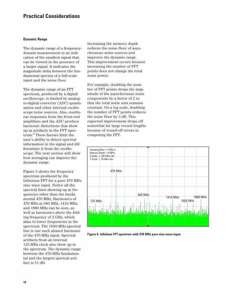
Sampling Rate = 4 GSa/sMemory Depth = 8 MPtsX Scale = 200 MHz/divY Scale = 20 dBm/div

125 MHz1410 MHz

1650 MHz1880 MHz

940 MHz

Figure 5. Infiniium FFT spectrum with 470 MHz pure sine wave input

Practical Considerations

Dynamic Range

The dynamic range of a frequency-domain measurement is an indi-cation of the smallest signal thatcan be viewed in the presence ofa larger signal. It indicates themagnitude delta between the fun-damental spectra of a full-scaleinput and the noise floor.

The dynamic range of an FFTspectrum, produced by a digitaloscilloscope, is limited by analog-to-digital converter (ADC) quanti-zation and other internal oscillo-scope noise sources. Also, nonlin-ear responses from the front-endamplifiers and the ADC produceharmonic distortions that showup as artifacts in the FFT spec-trum.3 These factors limit theuser’s ability to detect spectralinformation in the signal and dif-ferentiate it from the oscillo-scope. The next section will showhow averaging can improve thedynamic range.

Figure 5 shows the frequencyspectrum produced by theInfiniium FFT for a pure 470 MHzsine wave input. Notice all thespectral lines showing up at fre-quencies other than the funda-mental 470 MHz. Harmonics of470 MHz at 940 MHz, 1410 MHz,and 1880 MHz can be seen, aswell as harmonics above the fold-ing frequency of 2 GHz, whichalias to lower frequencies in thespectrum. The 1650-MHz spectralline is one such aliased harmonicof the 470-MHz input. Spectralartifacts from an internal125-MHz clock also show up inthe spectrum. The dynamic rangebetween the 470-MHz fundamen-tal and the largest spectral arti-fact is 51 dB.

Increasing the memory depthreduces the noise floor of asyn-chronous noise sources andimproves the dynamic range. This improvement occurs becauseincreasing the number of FFTpoints does not change the totalnoise power.

For example, doubling the num-ber of FFT points drops the mag-nitude of the asynchronous noisecomponents by a factor of 2 sothat the total noise sum remainsconstant. On a log scale, doublingthe number of FFT points reducesthe noise floor by 3 dB. Thisexpected improvement drops offsomewhat for large record lengthsbecause of round-off errors incomputing the FFT.

11

Practical Considerations

250 MHz

Sampling Rate = 4 GSa/sVertical Scale = 20 dBm/div

Memory Depth = 1024 ptsMemory Depth = 16,400,000 pts

Figure 6. Infiniium FFT spectrum showing how deep memory reduces thenoise level

Dynamic Range continued

Figure 6 shows the effect ofincreasing the FFT record lengthon dynamic range. The blue FFTtrace is acquired on an Infiniiumwith a memory depth of 1024points. The green FFT trace isacquired with a memory depth of16,400,000 points. Both areacquired at 4 GSa/s. Notice thatthe noise floor drops about 30 dBfor the deep-memory FFT, reveal-ing spectral data that are maskedwith only 1024 points. Unfor-tunately, some of the additionalspectral lines that become visiblewith deep memory are due to theoscilloscope and are not actuallypresent in the signal.

Digital oscilloscopes sometimesinclude effective bits in theirspecifications. Effective bits is ameasure of the signal-to-noiseratio (SNR). SNR is the ratio ofthe signal power to the total noisepower. It is typically computed inthe time domain using sine wavecurve fitting.4 SNR can be calcu-lated from effective bits using thefollowing equation:5

Equation 11

The effective bits measurement istypically worse with fast-slewinginputs, so it is often specified atboth high and low frequencies.Infiniium uses an 8-bit ADC.Using equation 11, an ideal 8-bitADC has an SNR of 50 dB.

SNR = Eff Bits * 6.02 + 1.8 dB

12

0

-10

-20

-30

-90

-80

-70

-60

-50

-40

-1000 0.50.450.40.350.30.250.20.150.10.05

1024 Pt. FFT Spectrum for Ideal 8-bit ADC

FREQ (HZ)

MA

GN

ITU

DE

(dB

)

Figure 7. Compare this 1024-point FFT spectrum for an ideal 8-bit ADC withthe 1024-point FFT in figure 6

Practical Considerations

Dynamic Range continued

Figure 7 shows a 1024-point FFTspectrum for an ideal 8-bit ADCwith a full-scale input. Noticewith 1024 points an SNR of 50 dB provides a dynamic rangeof about 70 dB. In contrast, asshown by the 1024-point FFT infigure 6, Infiniium has a dynamicrange of about 50 dB for a250 MHz, full-scale sine waveinput. This reduction of 20 dBfrom the ideal is caused by oscilloscope noise sources andnonlinear effects.

13

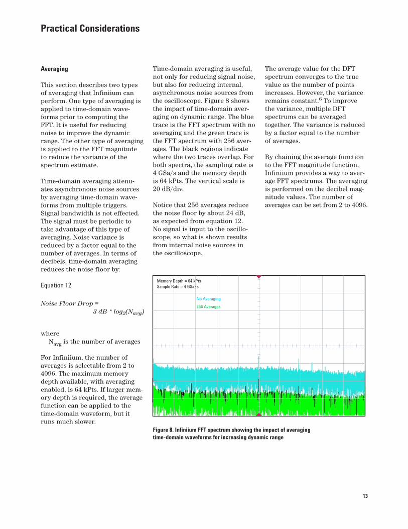
Memory Depth = 64 kPtsSample Rate = 4 GSa/s

No Averaging

256 Averages

Figure 8. Infiniium FFT spectrum showing the impact of averagingtime-domain waveforms for increasing dynamic range

Practical Considerations

Averaging

This section describes two typesof averaging that Infiniium canperform. One type of averaging isapplied to time-domain wave-forms prior to computing the FFT. It is useful for reducingnoise to improve the dynamicrange. The other type of averagingis applied to the FFT magnitudeto reduce the variance of thespectrum estimate.

Time-domain averaging attenu-ates asynchronous noise sourcesby averaging time-domain wave-forms from multiple triggers.Signal bandwidth is not effected.The signal must be periodic totake advantage of this type ofaveraging. Noise variance isreduced by a factor equal to thenumber of averages. In terms ofdecibels, time-domain averagingreduces the noise floor by:

Equation 12

whereNavg is the number of averages

For Infiniium, the number ofaverages is selectable from 2 to4096. The maximum memorydepth available, with averagingenabled, is 64 kPts. If larger mem-ory depth is required, the averagefunction can be applied to thetime-domain waveform, but itruns much slower.

Time-domain averaging is useful,not only for reducing signal noise,but also for reducing internal,asynchronous noise sources fromthe oscilloscope. Figure 8 showsthe impact of time-domain aver-aging on dynamic range. The bluetrace is the FFT spectrum with noaveraging and the green trace isthe FFT spectrum with 256 aver-ages. The black regions indicatewhere the two traces overlap. Forboth spectra, the sampling rate is4 GSa/s and the memory depth is 64 kPts. The vertical scale is20 dB/div.

Notice that 256 averages reducethe noise floor by about 24 dB, as expected from equation 12. No signal is input to the oscillo-scope, so what is shown resultsfrom internal noise sources in the oscilloscope.

Noise Floor Drop = 3 dB * log2(Navg)

The average value for the DFTspectrum converges to the truevalue as the number of pointsincreases. However, the varianceremains constant.6 To improvethe variance, multiple DFT spectrums can be averagedtogether. The variance is reducedby a factor equal to the number of averages.

By chaining the average functionto the FFT magnitude function,Infiniium provides a way to aver-age FFT spectrums. The averagingis performed on the decibel mag-nitude values. The number ofaverages can be set from 2 to 4096.

14

Practical Considerations

Memory Depth = 32 kPts

Non-averaged FFT Magnitude

Averaged FFT Magnitude, 16 Averages

Figure 9. Averaged FFT spectrums reduce variance

Averaging continued

Figure 9 shows the effect of aver-aging FFT spectrums. The greenspectrum trace, function 2, is notaveraged. The purple spectrumtrace, function 3, results fromaveraging function 2 sixteen

times. The black regions indicatewhere function 2 and function 3overlap. It is clear from figure 9that this type of averagingreduces the variance of the FFTspectrum but does not improvedynamic range.

15

Window Selection

Infiniium provides three windowfunctions to choose from, rectan-gular, Hanning, and flattop (referto figure 3). By selecting the prop-er window function, more usefulinformation can be obtained fromthe FFT spectrum.

Although the rectangular windowhas the narrowest main lobe, it isnot generally used because theside lobes fall off gradually,obscuring neighboring spectra.The Hanning window is the mostcommon window used for viewingspectral content. The main lobewidth is twice that of the rectan-gular window, but the side lobesfall off sharply.

When making magnitude meas-urements on spectral data, theflattop window is the best choice.Because of the broad flat top itexhibits in the frequency domain,the amplitude of a spectral peakis very accurate. The maximumamplitude error due to spectralleakage, using the flattop window,is 0.1 dB. This is much better

Practical Considerations

than the maximum error for theHanning window, which is1.5 dB.3 The maximum erroroccurs when the center of themain lobe falls exactly halfwaybetween two frequency bins.However, the flattop window isnot always a good choice whentrying to resolve closely-spacedspectral lines because of thebroad main lobe.

Increasing the memory depthimproves the frequency resolu-tion of the FFT without reducingthe frequency span (refer to equa-tion 2). In terms of frequencybins, the window function lobewidth is constant. But the fre-quency width of each bin isinversely proportional to thenumber of points. So increasingthe number of points decreasesthe spectral line lobe widths andimproves the ability to resolveclosely-spaced spectral lines. Forexample, by doubling the memorydepth, the flattop windowresolves as well as the Hanningwindow does with half the memory depth.

16

Practical Considerations

Equivalent Time Sampling

Aliasing is always a potentialissue for a digital oscilloscope.The oscilloscope passes all fre-quencies out to the specified analog bandwidth. The rolloff isnot necessarily sharp, so thateven frequencies beyond thebandwidth can be passed on tothe ADC.

Without a low-pass cutoff filter,frequencies above the folding fre-quency are allowed to alias intothe frequency spectrum. Theproblem is more severe when thesampling rate is reduced. Ideally,for spectral analysis, a low-passanalog filter would be injected toattenuate all frequencies abovethe folding frequency. This, however, is not practical for a digital oscilloscope.

Equivalent time sampling can beused to increase the effectivesampling rate and reduce alias-ing. Infiniium uses a form ofequivalent time sampling referredto as random repetitive sam-pling. The signal must be periodicfor this sampling technique towork properly. A random repeti-tive record is built up over severalacquisitions. The time betweenthe sample clock and the triggerevent is carefully measured andused to place the samples fromeach acquisition. The accuracy ofmeasuring this time dictates howclosely the samples can be spaced.The inverse of the sample spacingis the effective sampling rate.

For the Infiniium deep-memoryoscilloscope, the minimum sam-ple spacing in equivalent time is4 ps, providing a maximum effec-tive sampling rate of 250 GSa/s.

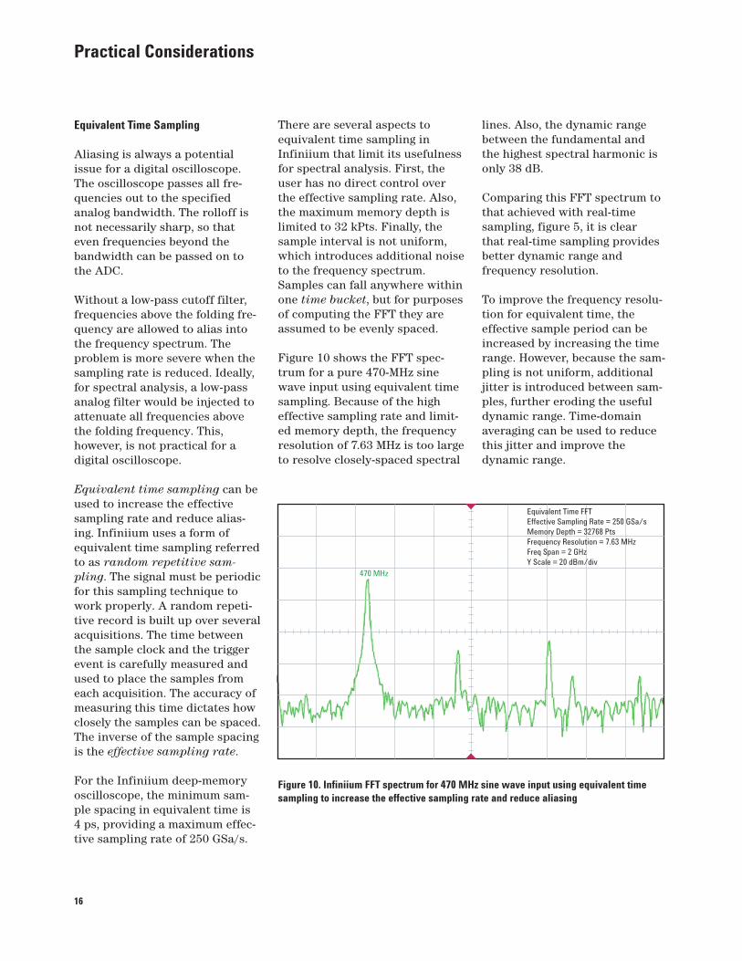
470 MHz

Equivalent Time FFTEffective Sampling Rate = 250 GSa/sMemory Depth = 32768 PtsFrequency Resolution = 7.63 MHzFreq Span = 2 GHzY Scale = 20 dBm/div

Figure 10. Infiniium FFT spectrum for 470 MHz sine wave input using equivalent timesampling to increase the effective sampling rate and reduce aliasing

There are several aspects toequivalent time sampling inInfiniium that limit its usefulnessfor spectral analysis. First, theuser has no direct control overthe effective sampling rate. Also,the maximum memory depth islimited to 32 kPts. Finally, thesample interval is not uniform,which introduces additional noiseto the frequency spectrum.Samples can fall anywhere withinone time bucket, but for purposesof computing the FFT they areassumed to be evenly spaced.

Figure 10 shows the FFT spec-trum for a pure 470-MHz sinewave input using equivalent timesampling. Because of the higheffective sampling rate and limit-ed memory depth, the frequencyresolution of 7.63 MHz is too largeto resolve closely-spaced spectral

lines. Also, the dynamic rangebetween the fundamental and the highest spectral harmonic isonly 38 dB.

Comparing this FFT spectrum tothat achieved with real-time sampling, figure 5, it is clear that real-time sampling providesbetter dynamic range and frequency resolution.

To improve the frequency resolu-tion for equivalent time, the effective sample period can beincreased by increasing the timerange. However, because the sam-pling is not uniform, additionaljitter is introduced between sam-ples, further eroding the usefuldynamic range. Time-domainaveraging can be used to reducethis jitter and improve thedynamic range.

17

Application

Characterizing an AM Signal

This section describes a real-world application for a deep-memory oscilloscope FFT. Theapplication involves measuringthe characteristics of an ampli-tude-modulated (AM) signal. Thecharacteristics of interest are thecarrier frequency, fo, modulationfrequency, fm, and modulationindex, a.3

The spectrum of an AM signalcontains all the information nec-essary to compute these parame-ters. Figure 11 shows the spec-trum of a typical AM signal withsinusoidal modulation. The cen-ter spectral line represents thecarrier and the sidebands resultfrom the modulation. The modu-lation frequency is the differencebetween the carrier frequencyand one of the sidebands. Themodulation index is a measure ofthe amplitude difference betweenthe carrier signal and the modula-tion signal. It can be computedfrom the magnitude delta, AdB,between the carrier and modula-tion sidebands, and is given bythe following equation:

Equation 13

When the modulation frequencyis a small percentage of the carri-er frequency, a high resolutionFFT spectrum is necessary to dis-tinguish the sidebands from the carrier.

For this example, an AgilentTechnologies 33250A functiongenerator is used to generate anAM signal with the followingparameters:

• Carrier frequency = 77 MHz• Modulation frequency = 1 kHz• AM depth = 2%• Shape = Sine

where the AM depth is equal tothe modulation index. Notice that the modulation frequency is 0.0013% of the carrier frequency. Differentiating themodulation from the carrier will require a high-resolution frequency spectrum.

AM Signal Spectrum

fo-fm fo fo+fmf

Figure 11. The spectrum of an AM signal with sinusoidal modulation

a = 2x10(AdB / 20)

18

Application

Selecting Sampling Rate and Memory Depth

The first task in setting up theoscilloscope to make this meas-urement is to select the samplingrate and memory depth. To pre-vent aliasing, the sampling rate,Fs, is set to a value greater thantwice the Nyquist frequency of77 MHz + 1 kHz. Also, for betterresolution, the minimum avail-able sampling rate that meets thiscriteria is selected. For Infiniium,the next available sampling rate,which is greater than twice theNyquist frequency, is 200 MSa/s.

To obtain the most accuratemeasurement of the modulationindex, a flattop window is used.The flattop window is 8 binswide, so to clearly distinguish themodulation sidebands requires afrequency resolution of 1 kHzdivided by 8. Using this fact andreferring to equation 2 for com-puting the frequency resolution,the following equation for com-puting the minimum number ofpoints is derived:

Equation 14

whereF is the frequency resolutionand W is the window main-lobe-width in bins

For this example, since the FFTupdate rate is not an issue, thememory depth is set to 8 MPts,which exceeds the minimumrequirement and provides a fre-quency resolution of 23.8 Hz.

Scaling Time and Frequency

The next task is to scale the oscil-loscope time and frequency axes.Recalling that the FFT is onlycomputed for onscreen points,the memory bar at the top of thescreen is used to set the timerange so that all the captureddata is onscreen. Using equation10, the time/div must be set to a value greater than or equal to 4 ms/div.

In this example, the time/div isset to 5 ms/div. The frequencyaxis is scaled so that the carrierfrequency is centered and thesidebands are separated from thecarrier by one division.

N ≥ = FsF

= = 1.6 MPtsFs

ƒm

W

200 MSa/s1 kHz

8

Horizontal Scale ≥

= 4ms / div8 MPts

10 x 200 MSa/s

19

Application

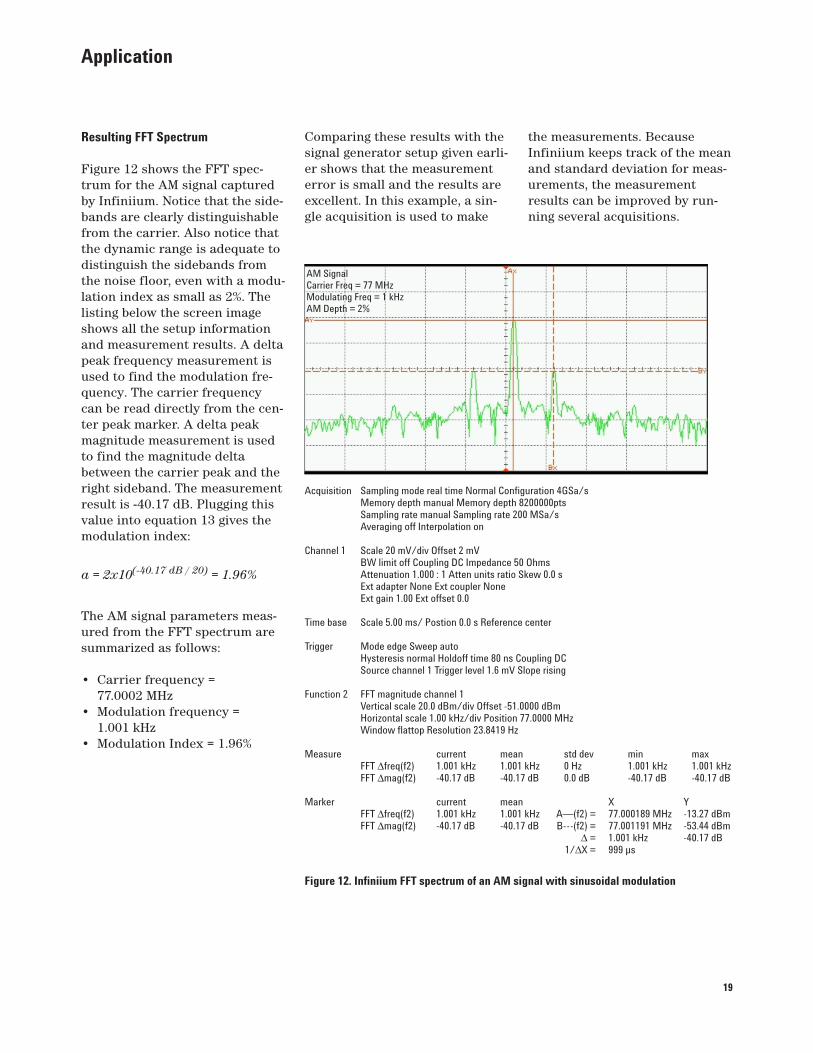
Resulting FFT Spectrum

Figure 12 shows the FFT spec-trum for the AM signal capturedby Infiniium. Notice that the side-bands are clearly distinguishablefrom the carrier. Also notice thatthe dynamic range is adequate todistinguish the sidebands fromthe noise floor, even with a modu-lation index as small as 2%. Thelisting below the screen imageshows all the setup informationand measurement results. A deltapeak frequency measurement isused to find the modulation fre-quency. The carrier frequencycan be read directly from the cen-ter peak marker. A delta peakmagnitude measurement is usedto find the magnitude deltabetween the carrier peak and theright sideband. The measurementresult is -40.17 dB. Plugging thisvalue into equation 13 gives themodulation index:

The AM signal parameters meas-ured from the FFT spectrum aresummarized as follows:

• Carrier frequency =77.0002 MHz

• Modulation frequency =1.001 kHz

• Modulation Index = 1.96%

AM SignalCarrier Freq = 77 MHzModulating Freq = 1 kHzAM Depth = 2%

a = 2x10(-40.17 dB / 20) = 1.96%

Comparing these results with thesignal generator setup given earli-er shows that the measurementerror is small and the results areexcellent. In this example, a sin-gle acquisition is used to make

the measurements. BecauseInfiniium keeps track of the meanand standard deviation for meas-urements, the measurementresults can be improved by run-ning several acquisitions.

Acquisition Sampling mode real time Normal Configuration 4GSa/sMemory depth manual Memory depth 8200000ptsSampling rate manual Sampling rate 200 MSa/sAveraging off Interpolation on

Channel 1 Scale 20 mV/div Offset 2 mVBW limit off Coupling DC Impedance 50 OhmsAttenuation 1.000 : 1 Atten units ratio Skew 0.0 sExt adapter None Ext coupler NoneExt gain 1.00 Ext offset 0.0

Time base Scale 5.00 ms/ Postion 0.0 s Reference center

Trigger Mode edge Sweep autoHysteresis normal Holdoff time 80 ns Coupling DCSource channel 1 Trigger level 1.6 mV Slope rising

Function 2 FFT magnitude channel 1Vertical scale 20.0 dBm/div Offset -51.0000 dBmHorizontal scale 1.00 kHz/div Position 77.0000 MHzWindow flattop Resolution 23.8419 Hz

Measure current mean std dev min maxFFT ∆freq(f2) 1.001 kHz 1.001 kHz 0 Hz 1.001 kHz 1.001 kHzFFT ∆mag(f2) -40.17 dB -40.17 dB 0.0 dB -40.17 dB -40.17 dB

Marker current mean X YFFT ∆freq(f2) 1.001 kHz 1.001 kHz A––(f2) = 77.000189 MHz -13.27 dBmFFT ∆mag(f2) -40.17 dB -40.17 dB B---(f2) = 77.001191 MHz -53.44 dBm

∆ = 1.001 kHz -40.17 dB1/∆X = 999 µs

Figure 12. Infiniium FFT spectrum of an AM signal with sinusoidal modulation

Agilent Technologies’ Test and Measurement Support, Services, and AssistanceAgilent Technologies aims to maximize the value you receive, while minimizing your risk andproblems. We strive to ensure that you get the test and measurement capabilities you paidfor and obtain the support you need. Our extensive support resources and services can helpyou choose the right Agilent products for your applications and apply them successfully.Every instrument and system we sell has a global warranty. Support is available for at leastfive years beyond the production life of the product. Two concepts underlie Agilent's overallsupport policy: "Our Promise" and "Your Advantage."

Our PromiseOur Promise means your Agilent test and measurement equipment will meet its advertisedperformance and functionality. When you are choosing new equipment, we will help youwith product information, including realistic performance specifications and practical rec-ommendations from experienced test engineers. When you use Agilent equipment, we canverify that it works properly, help with product operation, and provide basic measurementassistance for the use of specified capabilities, at no extra cost upon request. Many self-help tools are available.

Your AdvantageYour Advantage means that Agilent offers a wide range of additional expert test and meas-urement services, which you can purchase according to your unique technical and businessneeds. Solve problems efficiently and gain a competitive edge by contracting with us for cal-ibration, extra-cost upgrades, out-of-warranty repairs, and on-site education and training, aswell as design, system integration, project management, and other professional engineeringservices. Experienced Agilent engineers and technicians worldwide can help you maximizeyour productivity, optimize the return on investment of your Agilent instruments and sys-tems, and obtain dependable measurement accuracy for the life of those products.

For more assistance with your testand measurement needs, or to findyour local Agilent office go to:

www.agilent.com/find/assist

Product specifications and descriptions in thisdocument subject to change without notice.

©Agilent Technologies, Inc. 2001 Printed in USA November 15, 20015988-4368EN

www.agilent.com

References

1 Allen Montijo, “Weigh the Alternatives for Spectral Analysis,” Test & Measurement World, November 1999, Vol. 19, No. 14

2 Alan V. Oppenheim and Ronald W. Schafer, Digital Signal Processing, Prentice-Hall, Inc., 1975

3 Robert A. Witte, Spectrum & Network Measurements, Noble Publishing, 2001

4 “Dynamic Performance Testing of A to D Converters,” Hewlett Packard Product Note 5180A-2

5 Martin B. Grove, “Measuring Frequency Response and Effective Bits Using Digital Signal Processing Techniques,” Hewlett Packard Journal, February 1992, Vol. 43, No.1

6 Steven M. Kay, Modern Spectral Estimation, Prentice Hall, 1988