Spectral Analysis of Stationary Solutions of the

Cahn–Hilliard Equation

Peter HOWARD

March 25, 2008

Abstract

For the Cahn–Hilliard equation on R, there are precisely three types of boundednon-constant stationary solutions: periodic solutions, pulse-type reversal solutions,and monotonic transition waves. We study the spectrum of the linear operator ob-tained upon linearization about each of these waves, establishing linear stability forall transition waves, linear instability for all reversal waves, and linear instability fora representative class of periodic waves. For the case of transitions, the author hasshown in previous work that linear stability implies nonlinear stability, and so nonlin-ear (phase-asymptotic) stability is established for such waves.

1 Introduction

We consider the Cahn–Hilliard equation on R,

ut = (M(u)(F ′(u) − κuxx)x)x, (1.1)

where κ > 0 is assumed constant, and throughout the analysis we will make the followingassumptions:

(H0) M ∈ C2(R) and F ∈ C4(R).

(H1) F has a double-well form: there exist real numbers α1 < α2 < α3 < α4 < α5 sothat F is strictly decreasing on (−∞, α1) and (α3, α5) and strictly increasing on (α1, α3) and(α5,+∞), and additionally F is concave up on (−∞, α2) ∪ (α4,+∞) and concave down on(α2, α4). The interval (α2, α4) is typically referred to as the spinodal region.

We note that for each F satisfying assumptions (H0)–(H1), there exists a unique pair

of values u1 and u2 (the binodal values) so that F ′(u1) = F (u2)−F (u1)u2−u1

= F ′(u2) and the linepassing through (u1, F (u1)) and (u2, F (u2)) lies entirely on or below F .

(H2) For u ∈ [u1, u2], M(u) ≥ m0 > 0.

1

For equation (1.1) under conditions (H0)–(H1), and for M(u) ≥ m0 > 0 for all u ∈ R,there exist precisely three types of bounded non-constant stationary solutions u(x): periodicsolutions, pulse-type reversal solutions for which u(±∞) = u±, u− = u+, and monotonictransition waves for which u(±∞) = u±, u− 6= u+ (see [3] and Theorems 1.1, 1.3, and 1.4here). We study the spectrum of the linear operator obtained upon linearization about eachof these, establishing linear stability for all transition waves, linear instability for all reversalwaves, and linear instability for a representative class of periodic waves. For the case oftransitions, the author has shown in [20] that linear stability implies nonlinear stability, andso nonlinear (phase-asymptotic) stability is established for such waves.

The Cahn–Hilliard equation—often augmented by a driving or reaction term—arises inthe study of several phenomena, including phase separation [8], growth and dispersal ofbiological populations [10], chemical reaction kinetics [28], image inpainting [4], and as themodulation equation for a viscous incompressible fluid under the action of an external forceon an infinite strip [34, 44]. Our analysis is particularly motivated by the study of spinodaldecomposition, a phenomenon in which rapid cooling of a homogeneously mixed binaryalloy causes separation to occur, resolving the mixture into regions of different crystallinestructure in which one component or another is dominant, with these regions separatedby steep transition layers. (For a general reference on spinodal decomposition, the reader isreferred to J. W. Cahn’s 1967 Institute of Metals Lecture, printed as [8].) More precisely, thisphase separation is typically considered to take place in two stages: First, a relatively fastprocess occurs in which the homogeneous mixture quickly begins to separate (this is the stageof spinodal decomposition), followed by a second coarsening process (sometimes referred toas ripening) during which the regions continue to broaden on a relatively slower timescale,and the maximum difference in concentrations of the two components continues to increase(though in practice this latter increase can be extremely small). (For particularly accessibleaccounts of experimental studies of this process, the reader is referred to [25, 26, 27, 31].)

In this context, u typically denotes one component of the binary alloy (or a convenientaffine transformation of this concentration), and the Cahn–Hilliard equation arises from theconservation law

ut + ∇ · −M(u)∇δE

δu = 0,

where M(u) denotes the mobility associated with component u and is typically assumedpositive, and E denotes the total free energy associated with u. The Cahn–Hilliard equationas considered here arises from these considerations and a form of E(u) proposed in 1958by Cahn and Hilliard, who were considering particularly the interfacial energy between twocomponents of a binary compound [9]. Taking F (u) to denote the bulk free energy densityassociated with a homogeneously arranged alloy with concentration u, Cahn and Hilliardposed the energy functional

E(u) =

∫

Ω

F (u) +κ

2|∇u|2dx, (1.2)

where in the setting of [9] Ω denotes a bounded open subset of R3, and the term κ

2|∇u|2

2

arises as a first order correction that accounts for interfacial energy. (In fact, the functionalE(u) was originally proposed by van der Waals in [45] as an appropriate energy for a two-phase system.) In the case of relatively high temperatures, F generally has a quadratic form,expressing that free energy is minimized by configurations that maximize entropy, and suchconfigurations correspond with values of u for which the components of the alloy are evenlymixed to the point allowed by mass conservation. On the other hand, as temperature drops,free energy increases at a rate proportional to entropy, and F can take on the double-well formof (H1). In this way, the original (high-temperature) homogeneous configuration u = uh canbecome unstable at the lower temperature, and consequently small perturbations from uh donot dissipate, but rather propagate with quite complicated dynamics. (See, for example, thenumerical calculations [5, 7, 12, 13, 32, 33].) Our goal in the current analysis is to determinethe stability or instability of stationary solutions u(x) to (1.1), and to interpret our resultsin the context of this nonlinear evolution. We note at the outset of our investigation that aclosely related result has already been established by Alexiades and Aifantis in [1]. Namely,the authors establish that reversal and periodic solutions to (1.1) are not minimizers of theenergy functional (1.2), and that transition waves are minimizers of this functional. (In fact,the authors work in a more general setting than the one described here, taking κ = κ(u) in(1.2), which is consistent with the derivation of Cahn and Hilliard.) In the case of transitionwaves, we combine the methods of [1] with a straightforward Evans function argument toestablish our spectral result. Our instability results, however, both for the case of reversalsand for the case of periodic solutions, are based entirely on Evans function techniques.

We observe at the outset that for any linear function G(u) = Au + B, we can replaceF (u) in (1.1) with H(u) = F (u) −G(u). If we take

G(u) =F (u2) − F (u1)

u2 − u1

(u− uh) + F (uh),

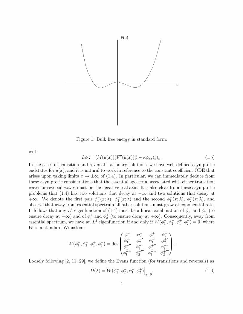
where uh is the unique value for which both F ′′(uh) < 0 and F ′(uh) = (F (u2)−F (u1))/(u2−u1), then H(u) has a local maximum H = 0 and local minima at the binodal values H(u1) =H(u2). Finally, replacing u with u+uh, we can shift H so that the local maximum is locatedat u = 0 (see Figure 1). We will refer to a double well function F (u) for which the localmaximum occurs at u = 0 and with equivalent local minima as standard form.

Upon linearization of (1.1) about the stationary solution u(x) (of any type), we obtainthe linear equation

vt = (M(u(x))(F ′′(u)v − κvxx)x)x, (1.3)

where we have used the observation that u(x) satisfies

F ′(u) − κuxx = C = constant.

The eigenvalue problem associated with (1.3) has the form

Lφ = λφ, (1.4)

3

F(u)

u

Figure 1: Bulk free energy in standard form.

withLφ := (M(u(x))(F ′′(u(x))φ− κφxx)x)x. (1.5)

In the cases of transition and reversal stationary solutions, we have well-defined asymptoticendstates for u(x), and it is natural to work in reference to the constant coefficient ODE thatarises upon taking limits x → ±∞ of (1.4). In particular, we can immediately deduce fromthese asymptotic considerations that the essential spectrum associated with either transitionwaves or reversal waves must be the negative real axis. It is also clear from these asymptoticproblems that (1.4) has two solutions that decay at −∞ and two solutions that decay at+∞. We denote the first pair φ−

1 (x;λ), φ−2 (x;λ) and the second φ+

1 (x;λ), φ+2 (x;λ), and

observe that away from essential spectrum all other solutions must grow at exponential rate.It follows that any L2 eigenfunction of (1.4) must be a linear combination of φ−

1 and φ−2 (to

ensure decay at −∞) and of φ+1 and φ+

2 (to ensure decay at +∞). Consequently, away fromessential spectrum, we have an L2 eigenfunction if and only if W (φ−

1 , φ−2 , φ

+1 , φ

+2 ) = 0, where

W is a standard Wronskian

W (φ−1 , φ

−2 , φ

+1 , φ

+2 ) = det

φ−1 φ−

2 φ+1 φ+

2

φ−1′

φ−2′

φ+1′

φ+2′

φ−1′′

φ−2′′

φ+1′′

φ+2′′

φ−1′′′

φ−2′′′

φ+1′′′

φ+2′′′

.

Loosely following [2, 11, 29], we define the Evans function (for transitions and reversals) as

D(λ) = W (φ−1 , φ

−2 , φ

+1 , φ

+2 )

∣

∣

∣

x=0. (1.6)

4

In the current setting D(λ) is not analytic in a neigborhood of the critical point λ = 0, butit can be defined analytically as a function of ρ =

√λ, and we set

D(ρ) := D(λ).

The function ux(x) is an eigenfunction of L associated with the eigenvalue λ = 0, and so weknow immediately that D(0) = 0. Our condition for spectral (and linear) stability requiresthat this be the only zero of D with non-negative real part. Following [20], we will say thata transition or reversal wave is spectrally stable if the following condition is satisfied:

(D): The Evans function D(λ) has precisely one zero in Re λ ≤ 0, necessarily at 0,and Dρρ(0) 6= 0.

We are now in a position to state the following theorems on spectral and nonlinearstability for transition waves, and on spectral instability for reversals.

Theorem 1.1 (Spectral stability for transition waves.). For equation (1.1), under conditions(H0)–(H2), there exist two transition wave solutions u(x) and u(−x), both of which arestrictly monotonic, and both of which approach the binodal values u1 < u2:

limx→−∞

u(x) = u1; limx→+∞

u(x) = u2.

Under the additional condition M(u) ≥ m0 > 0 for all u ∈ R, these are the only transitionwave solutions to (1.1). Moreover, each of these transition waves is spectrally stable in thesense that (D) is satisfied.

Combined with the nonlinear analysis of [20], we have the following theorem on stabilityfor transition wave solutions to the Cahn–Hilliard equation.

Theorem 1.2 (Nonlinear stability for transition waves). Under the conditions of Theorem1.1, the transition waves u(x) and u(−x) described there are nonlinearly stable as follows:For Holder continuous initial perturbations u(0, x) − u ∈ C0+γ(R), γ > 0, with

|u(0, x) − u(x)| ≤ E0(1 + |x|)− 3

2 ,

for some E0 sufficiently small, there exists some local tracking function δ(t) so that

|u(t, x+ δ(t)) − u(x)| ≤ CE0(1 + |x| +√t)−

3

2 ,

with

δ(t) = − 1

u+ − u−

∫ +∞

−∞(u(0, x) − u(x))dx+ O(t−

1

4 ).

Remark 1.1. For a more complete statement of Theorem 1.2, and for details regarding thelocal tracking function δ(t)—which is not a Dirac delta function—the reader is referred to[20].

5

For reversal solutions we have the following theorem on spectral (and linear) instability.

Theorem 1.3 (Spectral instability for reversal waves.). For equation (1.1), under conditions(H0)–(H2), let u3 and u4 denote real numbers fixed between the binodal values such thatu1 < u3 < u4 < u2, and suppose that one of the following holds:

F ′(u3) =F (u4) − F (u3)

u4 − u3> F ′(u4); or F ′(u3) >

F (u4) − F (u3)

u4 − u3= F ′(u4).

In the first case, there exists a reversal solution satisfying

limx→±∞

u(x) = u3; and maxx∈R

u(x) = u4,

(here, u3 must lie outside the spinodal region), while for the second

limx→±∞

u(x) = u4; and minx∈R

u(x) = u3

(here, u4 must lie outside the spinodal region). Under the additional assumption M(u) ≥m0 > 0 for all u ∈ R, this categorizes all possible reversal solutions to (1.1). Moreover, eachsuch solution is linearly unstable with a positive real eigenvalue.

In the case of periodic stationary solutions, we loosely follow the approach of Gardner[16, 17, 18], with additional aspects of the analysis taken from Oh and Zumbrun [35, 36],Schneider [41, 42, 43], and Papanicolaou [37, 39]. Letting u(x) be a periodic solution to (1.1)with period X, we proceed by searching for eigenfunctions of (1.4) with the particular formφ(x) = eiξxp(x), where ξ ∈ R and p(x) has period X. (A detailed explanation of the natureof this choice can be found, for example, on p. 171 of [38].) Upon substitution of this ansatzinto (1.4), we arrive at an eigenvalue problem for p on a bounded domain x ∈ [0, X],

Lξp = λp; p(k)(0) = p(k)(X), k = 0, 1, 2, 3, (1.7)

whereLξ := e−iξxLeiξx. (1.8)

We proceed now by constructing solutions to (1.7) in terms of a basis of solutions to (1.4)

φj4j=1 initialized by φ

(k−1)j (0;λ) = δk

j for k = 1, 3, 4, with (bφj)′(0;λ) = δj

2, where b(x) :=

F ′′(u(x)) and δkj denotes a standard Kronecker delta function. In particular, we create a

basis of solutions for (1.7) pj4j=1 through the relations pj(x;λ) = e−iξxφj(x;λ). Looking

for solutions

p(x) =

4∑

j=1

Vj(λ)pj(x;λ)

that satisfy the boundary conditions of (1.7), we conclude that there exists a solution to (1.7)if and only if there exists ξ ∈ R such that eiξX is an eigenvalue of the eigenvalue problem

M(λ;X)V = eiξXV ; V = (V1, V2, V3, V4)tr (1.9)

6

where M(λ;X) is the monodromy or Floquet matrix

M(λ;X) =

φ1(X;λ) φ2(X;λ) φ3(X;λ) φ4(X;λ)(bφ1)

′(X;λ) (bφ2)′(X;λ) (bφ3)

′(X;λ) (bφ4)′(X;λ)

φ′′1(X;λ) φ′′

2(X;λ) φ′′3(X;λ) φ′′

4(X;λ)φ′′′

1 (X;λ) φ′′′2 (X;λ) φ′′′

3 (X;λ) φ′′′4 (X;λ)

. (1.10)

Accordingly, we define the Evans function for periodic waves as

E(λ, ξ) := det(M(λ,X) − eiξXI). (1.11)

In most Evans function literature, this quantity is denoted D, and we only use E here todistinguish our Evans function for periodic waves from our Evans function for transition andreversal waves. It is clear from the discussion leading up to (1.11) that for periodic waves,L has an eigenvalue λ∗ whenever there exists ξ ∈ R so that E(λ∗, ξ) = 0.

Theorem 1.4 (Existence of periodic waves.). For equation (1.1), under conditions (H0)–(H2), let u3 and u4 denote real numbers fixed between the binodal values such that u1 < u3 <u4 < u2, and such that

F ′(u3) >F (u4) − F (u3)

u4 − u3

> F ′(u4).

Then there exists a non-constant periodic solution to (1.1) with minimum value u3 andmaximum value u4. Under the additional assumption M(u) ≥ m0 > 0 for all u ∈ R, thiscategorizes all possible non-constant periodic solutions to (1.1).

We now state an instability result for a restricted class of periodic solutions. In provingthis result, we will state a general condition for instability of all periodic waves from Theorem1.4, and the condition can readily be checked numerically on a case-by-case basis. In Theorem1.5, we address an important class of periodic waves for which the condition can be verifiedanalytically.

Theorem 1.5 (Spectral instability for periodic waves.). For equation (1.1), under conditions(H0)–(H2), suppose additionally that M(u) ≡ 1 and that F (u) in standard form is an evenfunction. Then for each u∗ ∈ (0, u2) there exists a unique periodic solution u(x) to (1.1)with minimum −u∗ and maximum +u∗. Moreover, this periodic solution is unstable with apositive real eigenvalue, provided F ′′′(u) ≥ 0 for u ∈ [0, u∗].

We note that the condition on F ′′′(u) is by no means necessary for instability, and weonly specify it because it can easily be checked, and because it is valid for the forms of Fmost frequently studied (see, for example, [1]). In particular, it is valid for polynomials ofthe form F (u) = au4 − bu2, where a and b are both positive constants.

Roughly speaking, our results can be interpreted in the context of spinodal decomposi-tion as follows. When the homogeneously mixed binary alloy is cooled, the constant solution

7

−10 −8 −6 −4 −2 0 2 4 6 8 10−1

−0.8

−0.6

−0.4

−0.2

0

0.2

0.4

0.6

0.8

1

x

Equil

ibri

um

Solu

tions

Periodic Solutions and Limiting Transition Wave

Figure 2: Stationary solutions of the Cahn–Hilliard equation.

u(t, x) = uh becomes unstable, and spinodal decomposition begins. If the natural perturba-tion to this homogeneous configuration is fairly random, then we might heuristically expect itto evolve toward small-amplitude periodic waves. (While this is only heuristic in the currentsetting, Grant has verified this picture in the case of bounded domains [14, 15].) Each ofthese periodic solutions is unstable, and so the solution moves away from them, coarseningfurther toward the stable transition wave. Though we do not make any effort to verify ithere, numerical experiments suggest that the periodic solutions become less stable as theiramplitudes near the binodal values (the endstates of the stable transition wave). In Figure2, we plot a number of different stationary solutions for the case of (1.1) with M ≡ 1, κ = 1,and F (u) = 1

8u4− 1

4u2, while in Figure 3, we plot the leading eigenvalue associated with these

waves as a function of amplitude (these eigenvalues were obtained numerically). For smallamplitudes, the eigenvalues are relatively large, and this corresponds with the relatively fastspinodal decomposition phase. As the amplitude grows, however, the leading eigenvaluesdecrease, and we enter the relatively slow coarsening phase. In this way, Figure 2 can almostbe viewed as a time evolution from the constant homogeneous state uh = 0 to the finaltransition front from −1 to +1. Along these lines, it’s interesting to compare Figure 2 withFigure 2 of [33], which depicts a numerical evolution of a perturbation of uh = 0 for (1.1)with M ≡ 1, κ = .001, and F (u) = 1

4u4 − 1

2u2.

8

0 0.1 0.2 0.3 0.4 0.5 0.6 0.7 0.8 0.9 10

0.01

0.02

0.03

0.04

0.05

0.06

0.07Leading eigenvalues as a function of amplitude

Le

ad

ing

Eig

en

valu

e

Amplitude

u=0 corresponds with constant state

u=1 corresponds with transition wave

Figure 3: Leading eigenvalues plotted as a function of magnitude.

2 Instability of Periodic waves

In this section, we develop a general condition for instability of the periodic solutions de-scribed in Theorem 1.4. Our approach will be through Taylor expansion of the Evans functionE(λ, ξ). We note at the outset that the periodic waves u(x) of Theorem 1.4 satisfy the ODE

κuxx = F ′(u) − F (u4) − F (u3)

u4 − u3, (2.1)

and that without loss of generality we will shift u(x) so that uxx(0) = 0.Our starting point will be the relation

E(λ, ξ) =

det

[φ1] − (eiξX − 1) [φ2] [φ3] [φ4][(bφ1)

′] [(bφ2)′] − (eiξX − 1) [(bφ3)

′] [(bφ4)′]

[φ′′1] [φ′′

2] [φ′′3] − (eiξX − 1) [φ′′

4][φ′′′

1 ] [φ′′′2 ] [φ′′′

3 ] [φ′′′4 ] − (eiξX − 1)

,

where [φk] := φk(X;λ) − φk(0;λ), and we recall the notation b(x) = F ′′(u(x)). As an initialsimplication, we observe that by integrating (1.4), we can obtain the general relationship

[φ′′′k ] =

1

κ[(bφk)

′] − λ

κM(u(X))

∫ X

0

φk(x;λ)dx. (2.2)

9

Upon substitution of (2.2) into E(λ, ξ), followed by the algebraic operation of dividing thesecond row in the matrix of E(λ, ξ) by κ and subtracting the result from row 4, we find thatE(λ, ξ) can be written as the determinant of

[φ1] − (eiξX − 1) [φ2] [φ3] [φ4][(bφ1)

′] [(bφ2)′] − (eiξX − 1) [(bφ3)

′] [(bφ4)′]

[φ′′1] [φ′′

2] [φ′′3] − (eiξX − 1) [φ′′

4]

− λκM0

∫

φ1 − λκM0

∫

φ2 + (eiξX−1)κ

− λκM0

∫

φ3 − λκM0

∫

φ4 − (eiξX − 1)

,

(2.3)where for notational brevity we have taken M0 = M(u(X)), and following the convention of[35, 36] we have written

∫

φk :=

∫ X

0

φk(x;λ)dx.

In our expansion, we will first consider the case ξ = 0, which corresponds with perturbationswith period X. In this case,

E(λ, 0) = − λ

κM0det

[φ1] [φ2] [φ3] [φ4][(bφ1)

′] [(bφ2)′] [(bφ3)

′] [(bφ4)′]

[φ′′1] [φ′′

2] [φ′′3] [φ′′

4]∫

φ1

∫

φ2

∫

φ3

∫

φ4

,

and we see immediately that E(0, 0) = 0, while

Eλ(0, 0) = − 1

κM0det

[φ1] [φ2] [φ3] [φ4][(bφ1)

′] [(bφ2)′] [(bφ3)

′] [(bφ4)′]

[φ′′1] [φ′′

2] [φ′′3] [φ′′

4]∫

φ1

∫

φ2

∫

φ3

∫

φ4

∣

∣

∣

λ=0. (2.4)

We turn our attention, then, to the evaluation of the φk at λ = 0. Upon setting λ = 0 in(1.4) and integrating twice, we find that for each k = 1, 2, 3, 4,

κφ′′k − b(x)φk = −M0

(

(bφk)′(0) − κφ′′′

k (0))

∫ x

0

dy

M(u(y))+ κφ′′

k(0) − b(0)φk(0).

In this way, we see that each of the φk(x; 0) can be obtained by the solution of a secondorder ODE:

κφ′′1 − b(x)φ1 = −b(0); φ1(0) = 1, (bφ1)

′(0) = 0

κφ′′2 − b(x)φ2 = −M0

∫ x

0

dy

M(u(y)); φ2(0) = 0, (bφ2)

′(0) = 1

κφ′′3 − b(x)φ3 = κ; φ3(0) = 0, (bφ3)

′(0) = 0

κφ′′4 − b(x)φ4 = κM0

∫ x

0

dy

M(u(y)); φ4(0) = 0, (bφ4)

′(0) = 0.

(2.5)

10

In our analysis, we will also make use of two important combinations, m(x) := κφ1(x; 0) +b(0)φ3(x; 0) and w(x) = κφ2(x; 0) + φ4(x; 0), which respectively satisfy

κm′′ − b(x)m = 0; m(0) = κ,m′(0) = −κb′(0)

b(0)

κw′′ − b(x)w = 0; w(0) = 0, w′(0) =κ

b(0).

(2.6)

By a standard variation of parameters representation, we can now understand each of theφk in terms of two linearly independent solutions to the homogeneous problem

κφ′′ − b(x)φ = 0. (2.7)

As is clear from (2.1), one solution to this equation is ux(x), while the second can be writtenin terms of ux(x) by reduction of order:

ψ(x) =

ux(x)∫ x

0dyu2

y0 ≤ x ≤ x1

ux(x)∫ x

2x1

dyu2

y+ 2K1

uxx(x1)ux(x) x1 ≤ x ≤ x2

−ux(x)∫ X

xdyu2

y+ 2ux(x)

(

uxx(x1)K2−uxx(x2)K1

uxx(x1)uxx(x2)

)

x2 ≤ x ≤ X

, (2.8)

where x1 < x2 denote the two places for which ux(xk) = 0, and

K1 := limx→x−

1

(

uxx(x)

∫ x

0

dy

u2y

+1

ux(x)

)

K2 := limx→x−

2

(

uxx(x)

∫ x

2x1

dy

u2y

+1

ux(x)

)

+ 2K1uxx(x2)

uxx(x1),

both of which are well defined. We note in particular, that ux(x) and ψ(x) are the solutionsof (2.7) with initial conditions ux(0) > 0, uxx(0) = 0 (the second by our choice of shift) andψ(0) = 0, ψ′(0) = 1/ux(0) > 0, and consequently W (ux(x), ψ(x)) ≡ 1, where W denotes astandard Wronskian.

We now have enough notation is place to state a result on the derivatives of E(λ, ξ).

Lemma 2.1. Under the assumptions of Theorem 1.4, and with u(x) as described there, we

11

have that E(λ, ξ) is analytic in a neighborhood of (0, 0), and that the following relations hold:

E(0, 0) = Eλ(0, 0) = Eλξ(0, 0) = 0,

Eξ(0, 0) = Eξξ(0, 0) = Eξξξ(0, 0) = 0; Eξξξξ(0, 0) = 24X4,

Eλλ(0, 0) = 2b(X)ψ′(X)

ux(0)κ3det

(∫

φ3

∫

w[φ3] [w]

)

×[(

∫ X

0

u(x) − u(0)

M(u(x))dx

)2

−∫ X

0

dx

M(u(x))

∫ X

0

(u(x) − u(0))2

M(u(x))dx

]

Eλξξ(0, 0) = 2X2

κux(X)

(

b(X)[w]h′(X) − [φ3]

∫ X

0

u(x) − u(0)

M(u(x))dx

)

+ 2X2

κ

[b(X)[φ′2]

M0

∫ X

0

w(x)dx−∫ X

0

dx

M(u(x))

∫ X

0

φ3(x; 0)dx]

Proof. First, by variation of parameters, we have

φ3(x; 0) = −ux(x)

∫ x

0

ψ(y)dy + ψ(x)(u(x) − u(0)), (2.9)

from which differentiation reveals the useful relation [φ′3] = 0. Likewise, we can show

[φ′2] =

ψ′(X)M0

κ

∫ X

0

u(x) − u(0)

M(u(x))dx. (2.10)

Additionally, we observe that w(x) = κux(0)b(0)

ψ(x), from which we find [w′] = 0.

Since m(x) and w(x) constitute a complete basis for (2.7), we have

ux(x) =ux(0)

κm(x) +

b′(0)ux(0)

κw(x)

= ux(0)φ1(x; 0) + b′(0)ux(0)φ2(x; 0) +b(0)

κux(0)φ3(x; 0) +

b′(0)ux(0)

κφ4(x; 0).

We can immediately conclude the linear dependencies

∫

φ1 + b′(0)

∫

φ2 +b(0)

κ

∫

φ3 +b′(0)

κ

∫

φ4 = 0

[φ(k)1 ] + b′(0)[φ

(k)2 ] +

b(0)

κ[φ

(k)3 ] +

b′(0)

κ[φ

(k)4 ] = 0,

(2.11)

for differentiation up to any order k = 0, 1, 2, .... Returning to (2.4), this linear dependenceclearly gives Eλ(0, 0) = 0.

We proceed next with the calculation of Eλλ(0, 0). In this case, we obtain a sum of fourdeterminants, each with a λ-derivative on a different row. We combine these determinants

12

by eliminating φ1 from each (with (2.11)), so that they are all in terms of the same threevariables. Finally, we perform an elementary row operation so that the columns are orderedin Wronskian fashion. The calculation is tedious but straightforward, and leads eventuallyto

1

2Eλλ(0, 0) =

1

κux(0)M0det

∫

h∫

φ2

∫

φ3

∫

φ4

[h] [φ2] [φ3] [φ4][(bh)′] [(bφ2)

′] [(bφ3)′] [(bφ4)

′][h′′] [φ′′

2] [φ′′3] [φ′′

4]

∣

∣

∣

λ=0,

whereh(x) := ux(0)(∂λφ1)(x; 0) + ux(0)b′(0)(∂λφ2)(x; 0)

+ ux(0)b(0)

κ(∂λφ3)(x; 0) + ux(0)

b′(0)

κ(∂λφ4)(x; 0),

(2.12)

and consequently(

M(u(x))(b(x)h− κhxx)x

)

x= ux(x); h(j)(0) = 0, j = 0, 1, 2, 3.

We note that the initial conditions on h(x) are clear from (2.12) and the fact that the initialconditions on the φk do not vary with λ. Upon integrating this last equation twice, andusing variation of parameters, we can derive the useful expression

h′(X) =ψ′(X)

κ

∫ X

0

(u(x) − u(0))2

M(u(x))dx. (2.13)

According to (2.5) and (2.12), we have

[φ′′2] =

1

κb(X)[φ2] −

M0

κ

∫ X

0

dx

M(u(x));

[φ′′3] =

1

κb(X)[φ3];

[φ′′4] =

1

κb(X)[φ4] +M0

∫ X

0

dx

M(u(x));

h′′(X) =1

κb(X)h− 1

κ

∫ X

0

u(x) − u(0)

M(u(x))dx.

(2.14)

Upon substitution of (2.14) into our determinant, we arrive at

1

2Eλλ(0, 0) =

1

κux(0)M0

× det

∫

h∫

φ2

∫

φ3

∫

φ4

h [φ2] [φ3] [φ4](bh)′ [(bφ2)

′] [(bφ3)′] [(bφ4)

′]

− 1κ

∫ X

0u(x)−u(0)M(u(x))

dx −M0

κ

∫ X

0dx

M(u(x))0 M0

∫ X

0dx

M(u(x))

∣

∣

∣

λ=0.

13

Combining this relation with the observations just following (2.9), we conclude

1

2Eλλ(0, 0) =

b(X)

ux(0)κ2

[ [φ′2]

M0

∫ X

0

u(x) − u(0)

M(u(x))dx− h′(X)

∫ X

0

dx

M(u(x))

]

det

(∫

φ3

∫

w[φ3] [w]

)

Finally, we use (2.10) and (2.13) to eliminate [φ′2] and h′(X), and we conclude

1

2Eλλ(0, 0) =

b(X)ψ′(X)

ux(0)κ3det

(∫

φ3

∫

w[φ3] [w]

)

×[(

∫ X

0

u(x) − u(0)

M(u(x))dx

)2

−∫ X

0

dx

M(u(x))

∫ X

0

(u(x) − u(0))2

M(u(x))dx

]

.

Here, the expression in square brackets is strictly negative by Cauchy–Schwartz.We proceed next with the expansion of E(λ, ξ) in ξ. We begin with (2.3), computing

E(0, ξ) and then expanding (eiξX − 1) in powers of ξ. In this expansion, which is straight-foward and omitted, the first non-zero coefficient is the coefficient of ξ4, and we find

E(0, ξ) = X4ξ4 + O(|ξ|5).

We next consider the case Eλ(0, ξ), for which we already have Eλ(0, 0) = 0. In additionto this we find that Eλξ(0, 0) = 0, and so we focus on the coefficient of ξ2. First, uponexpansion of (eiξX − 1) in (2.3), we observe two ways in which we can get terms of order ξ2:we can multiply the expression 1

2X2ξ2 by a term that does not involve ξ or we can have a

product of iξX with itself. We observe, however, that our condition Eλξ(0, 0) = 0 ensuresthat the former terms must sum to 0. (Precisely the same cancellation that leads to thisidentity annihilates those terms.) For the product terms, our approach will be to simplifyterms prior to differentiating in λ. If we write

E(λ, ξ) = A0(λ) + A1(λ)ξ + A2(λ)ξ2 + . . . , (2.15)

then

A2(λ) = −X2[

det

(

[φ1] [φ2 + 1κφ4]

b(X)[φ′1] b(X)[(φ2 + 1

κφ4)

′]

)

+ det

(

[φ1] [φ3][φ′′

1] [φ′′3]

)

+ det

(

[(b(φ2 + 1κφ4))

′] [(bφ3)′]

[(φ2 + 1κφ4)

′′] [φ′′3]

)

]

+λX2

κM0

[

det

(

[φ1] [φ4]∫

φ1

∫

φ4

)

+ det

(

[(bφ2)′] [(bφ4)

′]∫

φ2

∫

φ4

)

+ det

(

[φ′′3] [φ′′

4]∫

φ3

∫

φ4

)

]

.

14

We take a λ-derivative of this expression and set λ = 0 in the result to obtain

A′2(0) = −X2

[

det

(

∂λφ1 [φ2 + 1κφ4]

b(X)(∂λφ1)′ b(X)[(φ2 + 1

κφ4)

′]

)

+ det

(

[φ1] ∂λ(φ2 + 1κφ4)

b(X)[φ′1] b(X)(∂λ(φ2 + 1

κφ4))

′

)

+ det

(

∂λφ1 [φ3](∂λφ1)

′′ [φ′′3]

)

+ det

(

[φ1] ∂λφ3

[φ′′1] (∂λφ3)

′′

)

+ det

(

(b∂λ(φ2 + 1κφ4))

′ [(bφ3)′]

(∂λ(φ2 + 1κφ4)

′′ [φ′′3]

)

+ det

(

[(b(φ2 + 1κφ4))

′] (b∂λφ3)′

[(φ2 + 1κφ4)

′′] (∂λφ3)′′

)

]

+X2

κM0

[

det

(

[φ1] [φ4]∫

φ1

∫

φ4

)

+ det

(

[(bφ2)′] [(bφ4)

′]∫

φ2

∫

φ4

)

+ det

(

[φ′′3] [φ′′

4]∫

φ3

∫

φ4

)

]

.

In the calculation that follows, it will be convenient to focus separately on the terms thatcontain differentiation in λ (the first 6) and the terms that don’t (the last three). Upon

elimination of [φ1] by the substitution [φ1] = − b′(X)κ

[w]− b(X)κ

[φ3], we find that the summationof the first six terms is equivalent to

X2

κux(X)

(

b(X)[w]h′(X) − [φ3]

∫ X

0

u(x) − u(0)

M(u(x))dx

)

.

For the terms that do not contain differentiation in λ, we proceed by using (2.14) to eliminate[φ′′

3] and [φ′′4]. A short calculation leads to the expression

X2

κ

[b(X)[φ′2]

M0

∫ X

0

w(x)dx−∫ X

0

dx

M(u(x))

∫ X

0

φ3(x; 0)dx]

.

Combining these observations, we conclude

A′2(0) =

X2

κux(X)

(

b(X)[w]h′(X) − [φ3]

∫ X

0

u(x) − u(0)

M(u(x))dx

)

+X2

κ

[b(X)[φ′2]

M0

∫ X

0

w(x)dx−∫ X

0

dx

M(u(x))

∫ X

0

φ3(x; 0)dx]

.

This concludes the proof of Lemma 2.1.

We now have the following general condition for instability of periodic waves u(x) asdescribed in Theorem 1.4.

Lemma 2.2. Under the assumptions of Theorem 1.4, and with u(x) as described there,instability of u(x) is implied by the condition Eλξξ(0, 0) < 0.

Proof. Observing that the leading order of the eigenvalue problem (1.7) is independent of ξ,we can apply a standard perturbation argument to establish that there exists a continuous

15

curve λ∗(ξ) such that λ∗(0) = 0 and E(λ∗(ξ), ξ) = 0. (See [38], Sections 8 and 17.) In lightof this, we need only determine the leading order behavior of λ∗(ξ). We proceed, then, byTaylor expansion of E(λ, ξ):

E(λ, ξ) = E(0, 0) +∞

∑

k=1

1

k!(λ∂λ + ξ∂ξ)

kE(λ, ξ)∣

∣

∣

(λ,ξ)=(0,0)

=1

2Eλλ(0, 0)λ2 +

1

2Eλξξ(0, 0)λξ2 +

1

24Eξξξξ(0, 0)ξ4 + . . . ,

(2.16)

where we have included only those terms relevant to the calculation. Expanding λ∗(ξ) as apower series in ξ, we see immediately from the relation Eξξ(0, 0) = 0 that there is no termof order ξ. We take, then

λ∗(ξ) = a2ξ2 + O(ξ3).

Upon setting E(λ∗(ξ), ξ) = 0, and matching coefficients of powers of ξ, we find that the firstorder is ξ4, and that we have

1

2Eλλ(0, 0)a2

2 +1

2Eλξξ(0, 0)a2 +X4 = 0,

from which we find

a2 =−1

2Eλξξ(0, 0) ±

√

14Eλξξ(0, 0)2 − 2Eλλ(0, 0)X4

Eλλ(0, 0). (2.17)

We observe that in the event that Eλλ(0, 0) < 0, then regardless of the sign of Eλξξ(0, 0)we will have a branch of eigenvalues corresponding with a2 > 0, and consequently we willhave an interval of positive real eigenvalues. Indeed, this case appears to correspond withinstability with respect to perturbations of period X. In the special case that Eλλ(0, 0) = 0,we have

a2 = − 2X4

Eλξξ(0, 0),

so that instability is implied by the condition Eλξξ(0, 0) < 0. Finally, in the event thatEλλ(0, 0) > 0, there exists a solution to (2.17) with positive real part if and only if Eλξξ(0, 0) <0.

Though the sign of Eλξξ(0, 0) can be verified numerically for a given wave u(x), in thegenerality of Lemma 2.2 it is difficult to verify analytically. In the next section, we considera symmetric setting in which direct evaluation is possible.

2.1 The Symmetric Case

In this section, we consider the case in which F—following the transformation to standardform—is an even double well function. For each such F , the binodal values are u1 = −u2 and

16

u2, and for each u∗ ∈ (0, u2) there exists a unique periodic solution with minimum −u∗ andmaximum u∗. (These are by no means the only periodic solutions for such F ; see Theorem1.4). We refer to this as the symmetric case.

We can observe from (2.1) that we have considerable symmetry in this case. In particular,u(x) solves

ux(x) = ±√

2

κ(F (u(x)) − F (u∗)); u(0) = 0. (2.18)

(In the case that F has the polynomial form F (u) = au4 − bu2, this equation can be solvedexactly for the symmetric u(x) in terms of appropriate Jacobi elliptic functions.) Letting Xdenote the period of u(x), we can describe u(x) as follows: restricted to the interval [0, X/2],u(x) is even about the midpoint X/4, while on [0, X] u(x) is odd about the midpoint X/2.The following lemma, which can be proven by direct calculation from the general expressions,follows from these symmetries.

Lemma 2.3. Suppose the assumptions of Theorem 1.5 hold, and that u(x) is defined asthere, with additionally u(0) = 0. In this case, the basis functions φ1(x; 0) and φ3(x; 0) areboth periodic with period X, and the following relations hold:

uxx(0) = 0; b′(0) = F ′′′(u(0))ux(0) = 0;

∫ X

0

u(x)dx = 0;

∫ X

0

ψ(x)dx = 0,

with additionally

∫ X

0

φ3(x; 0)dx = 4

∫ X4

0

u(X/4)2 − u(x)2

u2x

dx− 4Ku(X4)2

uxx(X4)

; ψ(X) =4Kux(0)

uxx(X4),

where

K := limx→X−

4

uxx(X/4)

∫ x

0

dy

u2y

+1

ux(x)

.

Applying Lemma 2.3 to Eλλ(0, 0) and A′2(0), we find

1

2Eλλ(0, 0) = − 4KX

κ2uxx(X/4)

∫ X

0

u(x)2dx

∫ X

0

φ3(x; 0)dx, (2.19)

and additionally

1

2Eλξξ(0, 0) = A′

2(0) =4KX2

κuxx(X/4)

∫ X

0

u(x)2dx− X3

κ

∫ X

0

φ3(x; 0)dx. (2.20)

Our first consideration will be the stability index associated with perturbations whoseperiod is the same as that of the wave u(x). Recalling that Eλ(0, 0) = 0, and following [35],we define

Γ := sgn[

Eλλ(0, 0)]

× sgn[

limR∋λ→∞

E(λ; 0)]

. (2.21)

17

In the event that Γ = −1, there must exist a positive real value of λ so that E(λ, 0) = 0;that is, Γ = −1 corresponds with spectral instability with respect to perturbations that areperiodic with the same period as the wave u(x). On the other hand, if Γ = +1 we know onlythat E(λ; 0) does not cross 0 an odd number of times, and consequently we cannot generallyconclude anything about spectral stability.

Lemma 2.4. For equation (1.1), under conditions (H0)–(H2), and for M(u) ≡ 1, we have

sgn[

limR∋λ→∞

E(λ; 0)]

= +1,

where E(λ, ξ) is as defined in (1.11), we have

Proof of Lemma 2.4. The proof of this lemma is straightforward, based on standard ODEasymptotics, and so we only briefly sketch the argument. We mention at the outset thatthere is a more elegant method outlined in [35], but the method is less standard and moredetails would be required for completeness.

We proceed by the rescaling argument of [19]. More precisely, we change variables in

(1.4) to the stretched coordinate y = |λ| 14x, for which (1.4) becomes

−κϕ′′′′(y) =λ

|λ|ϕ+ |λ|−1a′(y/|λ|1/4)ϕ+ |λ|− 3

4 (−b′(y/|λ|1/4)

+ a(y/|λ|1/4))ϕ′ − |λ|− 1

2 b(y/|λ|1/4)ϕ′′(y),

where ϕ(y) := φ(y). We write this equation as a first order system

W ′ = A(λ)W + O(|λ|− 1

2 )W, (2.22)

where λ := λ/|λ|,

A(λ) :=

0 1 0 00 0 1 00 0 0 1

−λ/κ 0 0 0

,

and we remark that it is important to the argument that M is constant so that the orderterm is size |λ|−1/2. The eigenvalues of A(λ) are the four roots of µ4 = −λ/κ, and we order

them as µ1 = (−√

22− i

√2

2) 4

√

(λ/κ), µ2 = (−√

22

+ i√

22

) 4

√

(λ/κ), µ3 = (√

22− i

√2

2) 4

√

(λ/κ), and

µ4 = (√

22

+ i√

22

) 4

√

(λ/κ). Looking for solutions to (2.22) of the form W = eµ3xZ, we findthat Z satisfies the integral equation

Z(y) = e(A(λ)−µ3(λ))yZ(0) +

∫ y

0

e(A(λ)−µ3(λ))(y−z)O(|λ|−1/2)Z(z)dz. (2.23)

We observe now that we only require Z at the value y = 4

√

|λ|X (so that solutions to (1.4)can be evaluated at x = X), and we can carry out the integral over this bounded region

18

by taking a supremum of the integrand. In this way, a standard contraction mapping canbe closed for |λ| sufficiently large. In order to isolate a solution associated with µ3, we takeZ(0) to be the eigenvector of A associated with µ3, namely Z(0) = V3 = (1, µ3, µ

23, µ

33)

tr. Inthis way, we have

Z( 4

√

|λ|X) = V3 + O(|λ|− 1

4 ).

Upon returning to our original coordinates (and proceeding similarly in the additional cases),we find

φk(X;λ) = eµk(λ)X(Vk + O(|λ|− 1

4 )), (2.24)

where Vk = (1, µk, µ2k, µ

3k)

tr is the eigenvector associated with µk. If we set Φ(x;λ) to be astandard fundamental solution constructed from the φk, then we can write the monodromymatrix as M(λ) = Φ(X;λ)Φ(0;λ)−1. In particular, we now have

E(λ; 0) = det(Φ(X;λ)Φ(0;λ)−1 − Φ(0;λ)Φ(0;λ)−1) = det((Φ(X;λ) − Φ(0;λ))Φ(0;λ)−1)

=det(Φ(X;λ) − Φ(0;λ))

det Φ(0;λ)= Π4

k=1(eµk(λ)X − 1) + O(|λ|− 1

4 ).

The claimed result is an immediate consequence of this formula.

It is clear from (2.21) and Lemma 2.4 that the stability index associated with ξ = 0 issimply

Γ = sgn[

Eλλ(0, 0)]

.

According to (2.19), this can only be negative if

4KX

κ2uxx(X/4)

∫ X

0

u(x)2dx

∫ X

0

φ3(x; 0)dx > 0,

which since uxx(X/4) < 0 requires K∫ X

0φ3(x; 0)dx < 0.

Lemma 2.5. Under the assumptions of Lemma 2.3, and for the wave u(x) described there,positivity of the stability index Γ is implied by positivity of K.

Proof We need only combine (2.19) with Lemma 2.3. In particular, if K is positive, then

so is∫ X

0φ3(x; 0)dx.

In general, the sign of K is easily checked for a given function F . In addition to this, wecan prove the following result on the behavior of K for periodic waves whose maximum andminimum values are near the binodal values.

Lemma 2.6. Under the assumptions of Lemma 2.3, there exists ǫ > 0 so that for u2−u∗ < ǫ,we have K > 0.

19

Proof. We begin by observing that K can be written in the alternative form

K =1

ux(0)+

∫ X4

0

uxx(X/4) − uxx(x)

ux(x)2dx. (2.25)

According to (2.1) and (2.18) we can re-write this as

K =1

√

−(2/κ)F (u∗)+

1

2

∫ X4

0

(F ′(u∗) − F ′(u(x)))

(F (u(x)) − F (u∗))dx.

Finally, we make the change of variables y = u(x) to write

K(u∗) =

√

κ

2

[ 1√

−F (u∗)− 1

2

∫ u∗

0

F ′(y) − F ′(u∗)

(F (y) − F (u∗))3/2dy

]

.

Letting now us denote the positive spinodal value (i.e., F ′′(us) = 0), we observe that foru∗ > us, there exists some value u∗∗ < us so that F ′(u∗∗) = F ′(u∗) and for y ∈ [u∗∗, u∗],there holds F ′(y) − F ′(u∗) ≤ 0, in which case we have

∫ u∗

0

F ′(y) − F ′(u∗)

(F (y) − F (u∗))3/2dx ≤

∫ u∗∗

0

F ′(y) − F ′(u∗)

(F (y) − F (u∗))3/2dx.

For y ∈ [0, u∗∗], (F (y) − F (u∗)) is bounded below by F (u∗∗) − F (u∗). We have, then, theestimate

K(u∗) ≥√

κ

2

[ 1√

−F (u∗)− 1

2

1

(F (u∗∗) − F (u∗))3/2

∫ u∗∗

0

F ′(y) − F ′(u∗)dy]

=

√

κ

2

[ 1√

−F (u∗)− 1

2

F (u∗∗) − u∗∗F′(u∗)

(F (u∗∗) − F (u∗))3/2

]

.

In the limit as u∗ → u2, this approaches the limit

1√

−F (u2)> 0.

We conclude from this that at least for periodic waves whose maximum and minimumvalues are near the binodal values, we cannot rule out the possibility of spectral stabilitywith respect to perturbations that are periodic with the same period as the wave. Indeed,numerical calculations seem to indicate that such waves are stable with respect to suchperturbations.

We are now prepared to state a general lemma on the instability of symmetric periodicsolutions.

20

Lemma 2.7. Under the assumptions of Lemma 2.3, and for the wave u(x) described there,

instability of u(x) is implied by positivity of∫ X

0φ3(x; 0)dx.

Proof. Proceeding as in the proof of Lemma 2.2, we need only show that positivity of∫ X

0φ3(x; 0)dx implies that Eλξξ(0, 0) < 0. We begin by observing from (2.19) that with

∫ X

0φ3(x; 0)dx > 0, the only way we can have Eλλ(0, 0) > 0 is if K > 0. In this case, we can

see additionally from (2.20) that Eλξξ(0, 0) < 0. Moreover, we can compute

1

4Eλξξ(0, 0)2 − 2Eλλ(0, 0)X4 =

(X2b(X)w(X)ψ′(X)

κ2ux(0)

∫ X

0

u(x)2dx− X3

κ

∫ X

0

φ3(x; 0)dx)2

+4b(X)φ′(X)ω(X)X5

κ3ux(0)

∫ X

0

φ3(x; 0)dx

∫ X

0

u(x)2dx

=(X2b(X)w(X)ψ′(X)

κ2ux(0)

∫ X

0

u(x)2dx+X3

κ

∫ X

0

φ3(x; 0)dx)2

,

which is strictly positive for K and∫ X

0φ3(x; 0)dx both positive. The significance of this last

observation is that it verifies that we will have a real eigenvalue.

Theorem 1.5 can now be established by the following lemma on the positivity of theintegral

∫ X

0φ3(x; 0)dx.

Lemma 2.8. Let the assumptions of Lemma 2.3 hold, and suppose additionally that for u(x)as described there we have that F ′′′(u) ≥ 0 for all u ∈ (0, u∗). Then

∫ X

0

φ3(x; 0)dx > 0.

Proof. According to Lemma 2.3, we need only show positivity of the expression

∫ X4

0

u(X/4)2 − u(x)2

u2x

dx− Ku(X4)2

uxx(X4)

Upon substitution of the relation (2.25) for K, we find that this last expression is equivalentto

− 1

uxx(X/4)

[

∫ X4

0

uxx(X/4)u(x)2 − u(X/4)2uxx(x)

ux(x)2dx+

u(X/4)2

ux(0)

]

. (2.26)

Observing that −1/uxx(X/4) > 0, we need only establish positivity of the expression insquare brackets. Proceeding similarly as in the proof of Lemma 2.6, we set y = u(x), andwe find that this expression (in square brackets in (2.26)) is equivalent to

√

κ

2

[1

2

∫ u∗

0

y2F ′(u∗) − u2∗F

′(y)

(F (y) − F (u∗))3/2dy +

u2∗

√

−F (u∗)

]

. (2.27)

21

Finally, we observe that for functions F so that F ′′′(y) ≥ 0 for y ∈ [0, u∗], there holds

H(y) := y2F ′(u∗) − u2∗F

′(y) ≥ 0,

from which positivity of (2.27) follows. In order to understand this final inequality, weobserve that F ′′(0) < 0 for double-well F in standard form, and consequently H(y) is positivefor sufficiently small values of y. Moreover, for F ′′′(y) ≥ 0, H(y) is concave down for ally ∈ (0, u∗), while additionally H(u∗) = 0. This eliminates the possibility of a zero of Hbetween 0 and u∗, and thus it must be positive on the entire interval.

As discussed in the introduction, this condition on F ′′′(u) is not a necessary conditionfor instability. Indeed, it is clear from our proof that significantly less is required of F for(2.27) to be positive. Our choice of specifying Theorem 1.5 in this form is motivated bythe observation that this condition holds for the forms of F that make sense physically (see[1, 3]).

3 Transition and Reversal waves

In this section, we prove Theorems 1.1 and 1.3.

Proof of Theorem 1.1. We begin by observing that for the eigenvalue problem (1.4), withu(x) a transition wave, if we are away from essential spectrum the eigenfunctions φ(x;λ)must decay along with derivatives at exponential rate. Taking, then, λ 6= 0 away fromessential spectrum, we can integrate (1.4) to obtain the relation

∫ +∞

−∞φ(x;λ)dx = 0, (3.1)

for any L2 eigenfunction φ(x;λ). This justifies defining the exponentially decaying integratedvariable

w(x;λ) :=

∫ x

−∞φ(y;λ)dy,

which solves the eigenvalue problem

M(u(x))(F ′′(u(x))wx − κwxxx)x = λw. (3.2)

In particular, we observe that away from essential spectrum (also away from the eigenvalueλ = 0 embedded in essential spectrum), φ(x;λ) is an L2 eigenfunction of (1.4) if and only ifw(x;λ) is an L2 eigenfunction of (3.2). In this way, for λ 6= 0, the point spectrum of (1.4)corresponds precisely with the point spectrum of (3.2).

For (3.2), we divide by M(u(x)) and observe that the resulting equation,

(F ′′(u(x))wx − κwxxx)x = λ1

M(u(x))w, (3.3)

22

has a self-adjoint linear operator on the left-hand side. Consequently, the eigenvalues of both(1.4) and (3.2) are all real. Upon multiplication of (3.3) by w, integration over R, and anapplication of integration by parts, we obtain the relation

−∫ +∞

−∞wxHwxdx = λ

∫ +∞

−∞

1

M(u(x))w2, (3.4)

where H is the Schrodinger type operator

H := −κ∂2xx + F ′′(u(x)).

The operator H has an eigenvalue at λ = 0 associated with an eigenfunction ux(x) that isnever 0, and consequently λ = 0 is the lowest eigenvalue of H . It follows from the spectraltheorem that H is a positive operator, and we conclude from (3.4) λ ≤ 0. (A more detailedproof of the positivity of H is given in [1]; see also the relevant discussion on pp. 1246–1247of [40].)

For the eigenvalue at λ = 0, there remains to show that D′′(0) 6= 0. According to Lemma2.5 of [20] (restated in the current notation), we have

D′′(0) = −2(u+ − u−)

κM(u(0))det

φ−1 (x; 0) ux(x) φ+

2 (x; 0)

φ−1′(x; 0) uxx(x) φ+

2′(x; 0)

φ−1′′(x; 0) uxxx(x) φ+

2′′(x; 0)

∣

∣

∣

x=0. (3.5)

We must show that the functions φ−1 (x; 0), ux(x), and φ+

2 (x; 0) are linearly independent. Ifnot, then we can write φ−

1 (x; 0) as a linear combination of ux and φ+2 for x > 0 and conclude

from this that φ−1 (x; 0) is bounded at both ±∞. We will proceed by showing that in fact

neither φ−1 (x; 0) nor φ+

2 (x; 0) can be bounded at both ±∞.According to Lemma 2.1 of [20],

∂kxφ

−1 (x;λ) = eµ−

3(λ)x(µ−

3 (λ)k + O(e−α|x|))

∂kxφ

+2 (x;λ) = eµ−

2(λ)x(µ+

2 (λ)k + O(e−α|x|)),(3.6)

for k = 0, 1, 2, 3, and where

µ−3 (λ) =

√

b− −√

b2− − 4λc−2c−

; µ+2 (λ) = −

√

b+ −√

b2+ − 4λc+2c+

, (3.7)

and with b± := M(u±)F ′′(u±) and c± := κM(u±). In this way, we see that for each of thesolutions φ−

1 (x; 0), ux(x), and φ+2 (x; 0), we can integrate (1.4) to obtain

(F ′′(u)φ− κφxx)x = 0, (3.8)

where M(u) has been divided out. We must show, then, that any three solutions of (3.8)with the asymptotic behavior of φ−

1 (x; 0), ux(x), and φ+2 (x; 0) must necessarily be linearly

23

independent. Observing that ux is one solution of −κφ′′ + F ′′(u)φ, and that by reduction oforder a second solution is

φA(x) := ux(x)

∫ x

0

dy

uy(y)2,

we can construct a third, linearly independent, solution of (3.8) as the variation of parameterssolution of

F ′′(u)φ− κφxx = 1.

That is, we have a third solution

φB(x) = ux(x)

∫ x

0

u(y)

uy(y)2dy.

By construction, ux(x) decays at exponential rate at both ±∞, and φA(x) grows at expo-nential rate at both ±∞. Likewise, φB(x) grows at exponential rate at ∞ unless u+ = 0,in which case it grows at exponential rate at −∞. If we now look for a solution φ0(x) thatdoes not grow at either ±∞, we have

φ0(x) = α1ux(x) + α2φA(x) + α3φB(x).

In order to keep φ0(x) from growing at −∞, we require α2 + u−α3 = 0, while in order tokeep φ0(x) from growing at +∞ we require α2 +u+α3 = 0. Since u− 6= u+, we conclude thatα2 = α3 = 0, and consequently φ0(x) is a constant multiple of ux(x).

Proof of Theorem 1.3. For reversal waves, we proceed by defining and computing anappropriate stability index (see, for example, [6, 19]), though we note at the outset thatTheorem 1.3 can also be obtained by applying min-max methods to an appropriate integratedequation.

As in the case of transition fronts, the Evans function for reversals is given by

D(ρ) = W (φ−1 , φ

−2 , φ

+1 , φ

+2 )

∣

∣

∣

x=0, (3.9)

where the φ±k are the asymptotically decaying solutions of the eigenvalue problem (1.4) (as

described in the paragraph following (1.4)), and following [20], we take the convention

φ+1 (x; 0) = ux(x) = φ−

2 (x; 0). (3.10)

The remaining solutions φ−1 (x; 0) and φ+

2 (x; 0) both solve the third order equation

(F ′′(u(x)) − κφxx)x = 0, (3.11)

which has three linearly independent solutions: ux,

φA(x) = ux(x)

∫ x

−xdy

u′(y)2x < 0

∫ x

xdy

u′(y)2x > 0

,

24

where x is the unique positive value so that uxx(x) = 0, and where φA(0) can be defined tomake φA(x) continuous, and

φB(x) = ux(x)

∫ x

−xu(y)

u′(y)2dy x < 0

∫ x

xu(y)

u′(y)2dy x > 0

.

If we now expand φ−1 (x; 0) and φ+

2 (x; 0) as linear combinations of ux(x), φA(x), and φB(x),and insist on scalings such that

limx→−∞

φ−1 (x; 0) = lim

x→+∞φ+

2 (x; 0) = 1,

we find φ−1 (x; 0) = φ+

2 (x; 0) and

φ−1 (x; 0) = −F

′′(u∞)

κux(x)

∫ x

−xu(y)−u∞

u′(y)2dy x < 0

∫ x

xu(y)−u∞

u′(y)2x > 0

, (3.12)

where our notation here is

u(0) = u0; limx→±∞

u(x) = u∞;

i.e., u∞ is either u3 or u4 (q.v. the statement of Theorem 1.3) depending upon whether thereversal is up or down.

The identities φ−1 (x; 0) = φ+

2 (x; 0) and φ−2 (x; 0) = φ+

1 (x; 0) immediately give D(0) = 0and D′(0) = 0. Moreover, by combining these identities with the analyticity of φ+

1 (x; ρ) andφ−

2 (x; ρ2) in ρ2 we can conclude D′′(0) = 0, a degeneracy at ρ = 0. In this way, the directionof D(ρ) as ρ moves away from 0 is determined by the first non-zero derivative

D′′′(0) = 3W (∂ρφ−1 , ∂

2ρρ(φ

−2 − φ+

1 ), ux, φ+2 )

∣

∣

∣

x=0

+ 3W (φ−1 , ∂

2ρρ(φ

−2 − φ+

1 ), ux, ∂ρφ+2 )

∣

∣

∣

x=0.

(3.13)

In order to evaluate these determinants, we will employ a technical lemma that can beestablished by direct calculation losing techniques from the proof of Lemma 3.2 of [21] andLemma 3.3 of [22].

Lemma 3.1. Let T denote the linear operator

T := −c(x)∂3xxx + b(x)∂x − a(x),

wherec(x) = κM(u(x))

b(x) = M(u(x))F ′′(u(x))

a(x) = −M(u(x))F ′′′(u(x))ux(x).

25

Under the assumptions of Theorem 1.3, the solutions φ±k (x; 0) of the eigenvalue problem (1.4)

satisfy the following relations:

(i) Tφ±k (x; 0) ≡ 0, k = 1, 2

(ii) T∂φ−

1

∂ρ(x; 0) = b3/2

∞

(iii) T∂φ+

2

∂ρ(x; 0) = −b3/2

∞

(iv) T∂2φ−

2

∂ρρ(x; 0) = 2b2∞(u(x) − u∞)

(v) T∂2φ+

1

∂ρρ(x; 0) = 2b2∞(u(x) − u∞)

(vi) W (φ−1 , ux)(x; 0) = W (φ+

2 , ux)(x; 0) =F ′′(u∞)

κ(u(x) − u∞).

Employing Lemma 3.1, we find that for the first summand in (3.13) we have

W (∂ρφ−1 , ∂

2ρρ(φ

−2 − φ+

1 ), ux, φ+2 )(x; 0) = det

∂ρφ−1 ∂2

ρρ(φ−2 − φ+

1 ) u′ φ+2

(∂ρφ−1 )′ ∂2

ρρ(φ−2 − φ+

1 )′ u′′ φ+2′

(∂ρφ−1 )′′ ∂2

ρρ(φ−2 − φ+

1 )′′ u′′′ φ+2′′

− b3/2

∞

c(0)0 0 0

=b3/2∞

c(x)W (∂2

ρρ(φ−2 − φ+

1 ), u′, φ+2 )

=b3/2∞

c(x)W (∂2

ρρφ−2 , u

′, φ+2 ) − b

3/2∞

c(x)W (∂2

ρρφ+1 , u

′, φ+2 ).

(3.14)Observing the limit

limx→∞

W (∂2ρρφ

+1 , u

′, φ+2 )(x; 0) = 0,

we can write

W (∂2ρρφ

+1 , u

′, φ+2 )(x; 0) = −

∫ ∞

x

d

dyW (∂2

ρρφ+1 , u

′, φ+2 )(y; 0)dy.

Here,

d

dxW (∂2

ρρφ+1 , u

′, φ+2 )(x; 0) = det

∂2ρρφ

+1 u′ φ+

2

(∂2ρρφ

+1 )′ u′′ φ+

2′

−2b2∞

(u(x)−u∞)c(x)

0 0

= −2b2∞(u(x) − u∞)

c(x)W (u, φ+

2 ) =2b2∞F

′′(u∞)

κc(x)(u(x) − u∞)2,

26

where in this calculation we have used (v) and (vi) from Lemma 3.1. We conclude

W (∂2ρρφ

+1 , u

′, φ+2 )(x; 0)

∣

∣

∣

x=0= −2M(u∞)2F ′′(u∞)3

κ2

∫ ∞

0

(u(x) − u∞)2

M(u(x))dx. (3.15)

Proceeding similarly for the first Wronskian in the last line of (3.14), we find

W (∂2ρρφ

−2 , u

′, φ+2 )(x; 0)

∣

∣

∣

x=0=

2M(u∞)2F ′′(u∞)3

κ2

∫ 0

−∞

(u(x) − u∞)2

M(u(x))dx,

so that

W (∂ρφ−1 , ∂

2ρρ(φ

−2 − φ+

1 ), ux, φ+2 )(x; 0)

∣

∣

∣

x=0=

2M(u∞)7/2F ′′(u∞)9/2

κ3M(u0)

∫ +∞

−∞

(u(x) − u∞)2

M(u(x))dx.

(3.16)An equivalent contribution can similarly be shown to arise from the second summand in theexpression for D′′′(0), and we conclude

D′′′(0) =12M(u∞)7/2F ′′(u∞)9/2

κ3M(u0)

∫ +∞

−∞

(u(x) − u∞)2

M(u(x))dx.

We note in particular that D′′′(0) > 0. We are now in a position to define an appropriatestability index for this problem.

Definition 3.1. The stability index for a reversal wave u(x) is defined as

Γ = sgnD′′′(0) · limλ→∞

sgnD(λ).

Clearly the condition Γ = −1 guarantees the existence of a positive real eigenvalue, andsince we have D′′′(0) > 0, we need only understand the limit.

For λ real and sufficiently large, the behavior of solutions of the eigenvalue problem (1.4)are governed by the fourth order term, and we can proceed as in [6], in which the authorsanalyze thin-film equations of the general form

ut + f(u)x = (b(u)ux)x − (c(u)uxxx)x

(see also [23, 24]). In order to state the salient result from [6], we first observe that theeigenvalue problem (1.4) can be written as a first order system of four equations, withcomponents W1 = φ, W2 = φ′, W3 = φ′′, and W4 = φ′′′, and that this system can be writtenas W ′ = A(x;λ)W , and also in the asymptotic form

W ′ = A∞(λ)W + E(x;λ)W, (3.17)

whereA∞(λ) = lim

x→∞A(x;λ), (3.18)

and E(x;λ) decays at exponential rate in |x| as |x| → ∞. We are now in a position to adaptProposition 2.6 from [6] to the current setting. (For ease of reference, we adopt the notationof [6].)

27

Lemma 3.2. Let S+ denote the subspace of solutions of W ′ = A∞(λ)W that decay at +∞,and let U− denote the subspace of solutiosn of W ′ = A∞(λ)W that decay at −∞. In addition,let V +

j , j = 1, 2, denote a choice of basis vectors for S+, and let V −j , j = 3, 4, denote a choice

of basis vectors for U−. Then for λ > 0 real and sufficiently large

sgnD(λ) = sgn

det

(

V +11 V +

21

V +12 V +

22

)

det

(

V −31 V −

41

V −32 V −

42

)

∣

∣

∣

λ=0.

Here, the V ±jk are components of the vector V ±

j .

According to Lemma 3.2, the sign of D(λ) for large values of λ is determined by the basesof S+ and U− at λ = 0. By our choice of scaling convention φ−

1 (x; 0) and φ+2 (x; 0) approach 1

as x approaches −∞ and +∞. For the case u∞ > 0 ux(x) is positive for x < 0 and negativefor x > 0, while uxx(x) is positive for all |x| sufficiently large; for the case u∞ < 0 ux(x)is negative for x < 0 and positive for x > 0, while uxx(x) is negative for all |x| sufficientlylarge. We can conclude, for u∞ > 0,

sgn det

(

V +11 V +

21

V +12 V +

22

)

= limx→∞

sgn det

(

ux(x) φ+2 (x; 0)

uxx(x) φ+2′(x; 0)

)

= −1,

and similarly

sgn det

(

V −31 V −

41

V −32 V −

42

)

= limx→−∞

sgn det

(

φ−1 (x; 0) ux(x)

φ−1′(x; 0) uxx(x)

)

= +1, .

and each sign is opposite for u∞ < 0. We conclude that for λ real and sufficiently large

D(λ) < 0,

and according to the remark immediately following Definition 3.1 this guarantees that thereis a positive real eigenvalue associated with the reversal wave.

Acknowledgements. This research was partially supported by the National Science Foun-dation under Grant No. DMS–0500988.

References

[1] V. Alexiades and E. C. Aifantis, On the thermodynamic theory of fluid interfaces: in-finite intervals, equilibrium solutions, and minimizers, J. Colloid and Interface Science111 (1986) 119–132.

[2] J. Alexander, R. Gardner, and C. K. R. T. Jones, A topological invariant arising in theanalysis of traveling waves, J. Reine Angew. Math. 410 (1990) 167–212.

28

[3] E. C. Aifantis and J. B. Serrin, Equilibrium solutions in the mechanical theory of fluidmicrostructures, J. Colloid and Interface Science 96 (1983) 530–547.

[4] A. Bertozzi, S. Esedoglu, and A. Gillette, Analysis of a two-scale Cahn–Hilliard modelfor image inpainting, Preprint 2006.

[5] F. Bai, C. M. Elliot, A. Gardiner, A. Spence, and A. M. Stuart, The viscous Cahn–Hilliard equation. Part I: computations, Nonlinearity 8 (1995) 131–160.

[6] A. L. Bertozzi, A. Munch, M. Shearer, and K. Zumbrun, Stability of compressive andundercompressive thin film travelling waves: the dynamics of thin film flows, EuropeanJ. Appl. Math. 12 (2001) 253–291.

[7] J. W. Cahn, Phase separation by spinodal decomposition in isotropic systems, J. Chem-ical Physics 42 (1965) 93–99.

[8] J. W. Cahn, Spinodal Decomposition, Trans. Metallurgical Soc. AIME 242 (1968) 166–180.

[9] J. W. Cahn and J. E. Hilliard, Free energy of a uniform system I: Interfacial free energy,J. Chem. Phys. 28 (1958) 258–267.

[10] D. S. Cohen and J. D. Murray, A generalized diffusion model for growth and dispersalof a population, J. Math. Biology 12 (1981) 237–249.

[11] J. W. Evans, Nerve axon equations I–IV, Indiana U. Math. J. 21 (1972) 877–885; 22

(1972) 75–90; 22 (1972) 577–594; 24 (1975) 1169–1190.

[12] C. M. Elliot and D. A. French, Numerical studies for the Cahn–Hilliard equation forphase separation, IMA J. Appl. Math. 38 (1987) 97–128.

[13] D. J. Eyre, Systems of Cahn–Hilliard equations, SIAM J. Appl. Math. 53 (1993) 1686–1712.

[14] C. P. Grant, The dynamics of pattern selection for the Cahn–Hilliard equation, Ph.D.Thesis, The University of Utah, 1991, Advisor: Paul Fife.

[15] C. P. Grant, Spinodal decomposition for the Cahn–Hilliard equation, Comm. PartialDifferential Equations 18 (1993) 453–490.

[16] R. A. Gardner, On the structure of the spectra of periodic travelling waves, J. Math.Pures Appl. 72 (1993) 415–439.

[17] R. A. Gardner, Instability of oscillatory shock profile solutions of the generalizedBurgers–KdV equation, Physica D 90 (1996) 366–386.

29

[18] R. A. Gardner, Spectral analysis of long wavelength periodic waves and applications, J.Reine Angew. Math. 491 (1997) 149–181.

[19] R. Gardner and K. Zumbrun, The gap lemma and geometric criteria for instability ofviscous shock profiles, Comm. Pure Appl. Math. 51 (1998) 789–847.

[20] P. Howard, Asymptotic behavior near transition fronts for equations of generalizedCahn–Hilliard form, Commun. Math. Phys. 269 (2007) 765–808.

[21] P. Howard, Asymptotic behavior near planar transition fronts for the Cahn–Hilliardequation, Physica D 229 (2007) 123–165.

[22] P. Howard, Spectral analysis of planar transition fronts for the Cahn–Hilliard equation,to appear in J. Differential Equations.

[23] P. Howard and C. Hu, Pointwise Green’s function estimates toward stability for mul-tidimensional fourth order viscous shock fronts, J. Differential Equations 218 (2005)325–389.

[24] P. Howard and C. Hu, Nonlinear stability for multidimensional fourth order shock fronts,Arch. Rational Mech. Anal. 181 (2006) 201–260.

[25] J. M. Hyde, M. K. Miller, M. G. Hetherington, A. Cerezo, G. D. W. Smith, and C. M.Elliot, Spinodal decomposition in Fe–Cr alloys: experimental study at the atomic leveland comparison with computer models—II. development of domain size and compositionamplitude, Acta Metall. Mater. 43 (1995) 3403–3413.

[26] J. M. Hyde, M. K. Miller, M. G. Hetherington, A. Cerezo, G. D. W. Smith, and C. M.Elliot, Spinodal decomposition in Fe–Cr alloys: experimental study at the atomic leveland comparison with computer models—I. introduction and methodology, Acta Metall.Mater. 43 (1995) 3415–3426.

[27] S. A. Hill and B. Ralph, Continuous phase separation in a Nickel–Aluminum alloy, ActaMetall. 30 (1982) 2219–2225.

[28] B. A. Huberman, Striations in chemical reactions, J. Chem. Phys. 65 (1976) 2013–2019.

[29] C. K. R. T. Jones, Stability of the traveling wave solution of the FitzHugh–Nagumosystem, Trans. Amer. Math. Soc. 286 (1984) 431–469.

[30] J. S. Langer, Theory of spinodal decomposition in alloys, Annals of Physics 65 (1971)53–86.

[31] M. K. Miller, J. M. Hyde, M. G. Hetherington, A. Cerezo, G. D. W. Smith, and C. M.Elliot, Spinodal decomposition in Fe–Cr alloys: experimental study at the atomic leveland comparison with computer models—I. introduction and methodology, Acta Metall.Mater. 43 (1995) 3385–3401.

30

[32] W. McKinney, Thesis, Department of Mathematics, University of Tennessee, Knoxville,TN 1989. Partially reprinted in: N. Alikakos, P. W. Bates, and G. Fusco, Slow motionfor the Cahn–Hilliard equation in one space dimension, J. Differential Equations 90

(1991) 81–135.

[33] E. V. L. de Mello and O. T. dS. Filho, Numerical study of the Cahn–Hilliard equationin one, two, and three dimensions, Physica A 347 (2005) 429–443.

[34] A. A. Nepomniashchii, On stability of secondary flows of a viscous fluid in unboundedspace, J. Appl. Math. Mech. 40 (1976) 836–841.

[35] M. Oh and K. Zumbrun, Stability of periodic solutions of conservation laws with viscos-ity: analysis of the Evans function, Arch. Rational Mech. Anal. 166 (2003) 99–166.

[36] M. Oh and K. Zumbrun, Stability of periodic solutions of conservation laws with viscos-ity: pointwise bounds on the Green’s function, Arch. Rational Mech. Anal. 166 (2003)167–196.

[37] V. G. Papanicolaou, The spectral theory of the vibrating periodic beam, Commun. Math.Phys. 170 (1995) 359–373.

[38] G. V. Rozenblum, M. A. Shubin, and M. Z. Solomyak, Spectral theory of differentialoperators, in Encyclopedia of Mathematical Sciences Vol. 64, Partial Differential Equa-tions VII, Ed. M. A. Shubin.

[39] V. G. Papanicolaou, The periodic Euler–Bernoulli equation, Trans. AMS 355 (2003)3727–3759.

[40] M. Schatzman, On the stability of the saddle solution of Allen–Cahn’s equation, Pro-ceedings of the Royal Society of Edinburgh 125A (1995) 1241–1275.

[41] G. Schneider, Diffusive stability of spatial periodic solutions of the Swift–Hohenbergequation, Commun. Math. Phys. 178 (1996) 679–702.

[42] G. Schneider, Nonlinear diffusive stability of spatially periodic solutions—abstract the-orem and higher space dimensions, in: Proceedings of the International Conference onAsymptotics in Nonlinear Diffusive Systems (Sendai, 1997), 159–167, Tohoku Math.Publ., 8, Tohoku Univ., Sendai, 1998.

[43] G. Schneider, Nonlinear stability of Taylor vortices in infinite cylinders, Arch. RationalMech. Anal. 144 (1998) 121–200.

[44] G. Schneider, Cahn–Hilliard description of secondary flows of a viscous incompressiblefluid in an unbounded domain, Z. Angew. Math. Mech. 79 (1999) 615–626.

31

[45] J. D. van der Waals, The thermodynamic theory of capillarity under the hypothesis ofa continuous variation of density, (in Dutch) Verhandel. Konink. Akad. Weten. Ams-terdam (Sect. 1) 1 (1893). Published in English translation: J. Statistical Physics 20

(1979) 200–244, J. S. Rowlinson translator.

Peter HOWARDDepartment of MathematicsTexas A&M UniversityCollege Station, TX 77843phoward@math.tamu.edu

32