1

Compressive Spectral Estimation for Nonstationary

Random Processes

Alexander Jung, Georg Tauböck, Member, IEEE, and Franz Hlawatsch, Fellow, IEEE

Abstract— Estimating the spectral characteristics of a non-stationary random process is an important but challenging task,which can be facilitated by exploiting structural properties ofthe process. In certain applications, the observed processes areunderspread, i.e., their time and frequency correlations exhibit areasonably fast decay, and approximately time-frequency sparse,i.e., a reasonably large percentage of the spectral values are small.For this class of processes, we propose a compressive estimatorof the discrete Rihaczek spectrum (RS). This estimator combinesa minimum variance unbiased estimator of the RS (which is asmoothed Rihaczek distribution using an appropriately designedsmoothing kernel) with a compressed sensing technique thatexploits the approximate time-frequency sparsity. As a result ofthe compression stage, the number of measurements requiredfor good estimation performance can be significantly reduced.The measurements are values of the ambiguity function of theobserved signal at randomly chosen time and frequency lagpositions. We provide bounds on the mean-square estimationerror of both the minimum variance unbiased RS estimatorand the compressive RS estimator, and we demonstrate theperformance of the compressive estimator by means of simulationresults. The proposed compressive RS estimator can also be usedfor estimating other time-dependent spectra (e.g., the Wigner-Ville spectrum) since for an underspread process most spectraare almost equal.

Index Terms— Nonstationary random process, nonstationaryspectral estimation, time-dependent power spectrum, Rihaczekspectrum, Wigner-Ville spectrum, compressed sensing, basispursuit, cognitive radio.

I. INTRODUCTION

Estimating the spectral characteristics of a random process

is an important task in many signal analysis and processing

problems. Conventional spectral estimation based on the powerspectral density is restricted to wide-sense stationary and,

by extension, wide-sense cyclostationary processes [1], [2].

However, in many applications—including speech and audio,

communications, image processing, computer vision, biomed-

ical engineering, and machine monitoring—the signals of in-

terest cannot be well modeled as wide-sense (cyclo)stationary

processes. For example, in cognitive radio systems [3]–[5],

the receiver has to infer from the received signal the location

Copyright (©) 2013 IEEE. Personal use of this material is permitted.However, permission to use this material for any other purposes must beobtained from the IEEE by sending a request to pubs-permissions@ieee.org.

Alexander Jung, Georg Tauböck, and Franz Hlawatsch are with the Instituteof Telecommunications, Vienna University of Technology, A-1040 Vienna,Austria (e-mail: {ajung,gtauboec,fhlawats}@nt.tuwien.ac.at). This work wassupported by the FWF under grant S10603 (Statistical Inference) within theNational Research Network SISE and by the WWTF under grant MA 07-004(SPORTS). Parts of this work were previously presented at IEEE SSP 2009,Cardiff, Wales, UK, Aug.–Sept. 2009.

of unoccupied frequency bands (“spectral holes”) that can be

used for data transmission. Here, modeling the received signal

as a nonstationary process can be advantageous because it

potentially allows a faster estimation of time-varying changes

in band occupation [3].

For a general nonstationary process, a “power spectral

density” that is nonnegative and extends all the essential

properties of the conventional power spectral density is not

available [6]–[10]. Several different definitions of a “time-

dependent (or time-varying) power spectrum” have been pro-

posed in the literature, see [6]–[26] and references therein.

However, it has been shown [10], [24] that in the practically

important case of nonstationary processes with fast decay-

ing time-frequency (TF) correlations—so-called underspreadprocesses [10], [24]–[30]—all major spectra yield effectively

identical results, are (at least approximately) real-valued and

nonnegative, and satisfy several other desirable properties at

least approximately. Thus, in the underspread case, the specific

choice of a spectrum is of secondary theoretical importance

and can hence be guided by practical considerations such as

computational complexity.

Once a specific definition of time-dependent spectrum

has been adopted, an important problem is the estimation

of the spectrum from a single observed realization of the

process. This nonstationary spectral estimation problem is

fundamentally more difficult than spectral estimation in the

(cyclo)stationary case, because long-term averaging cannot be

used to reduce the mean-square error (MSE) of the estimate.

Formally, any estimator of a nonparametric time-dependent

spectrum can also be viewed as a TF representation of the

observed signal [7], [26], [31], [32]. Estimators have been

previously proposed for several spectra including the Wigner-

Ville spectrum and the Rihaczek spectrum (RS) (e.g., [7]–[9],

[21], [26], [33]–[41]).

In this paper, extending our work in [42], we propose

a “compressive” estimator of the RS that uses the recently

introduced methodology of compressed sensing (CS) [43],

[44]. The proposed estimator is suited to underspread pro-

cesses that are approximately TF sparse. The latter property

means that only a moderate percentage of the values of the

discrete RS are significantly nonzero. Both assumptions—

underspreadness and TF sparsity—are reasonably well satis-

fied in many applications, including, e.g., cognitive radio. We

consider the RS because it is the simplest time-dependent spec-

trum from a computational viewpoint, especially in the discrete

setting used. The proposed compressive estimator of the RS

is obtained by augmenting a basic noncompressive estimator

Copyright 2013 IEEE IEEE Trans. Inf. Theory, vol. 59, no. 5, May 2013, pp. 3117–3138

2

(a smoothed version of the Rihaczek distribution (RD), cf.

[7], [14], [26], [32], [33], [35], [38]–[41]) with a CS com-

pression-reconstruction stage. Algorithmically, our estimator

is similar to the compressive TF representation proposed in

[45], [46]. In fact, both our estimator and the TF representation

of [45], [46] are essentially based on a sparsity-regularized

inversion of the Fourier transform relationship between a TF

distribution and the values of the ambiguity function (AF)

taken at randomly chosen time lag/frequency lag locations.

The sparsity-regularization is achieved by requiring a small

ℓ1-norm of the resulting TF distribution. However, the set-

ting of [45], [46] is that of deterministic TF signal analysis

(more specifically, the goal is to improve the TF localization

properties of the Wigner distribution), whereas we consider a

stochastic setting, namely, spectral estimation for underspread,

approximately TF sparse, nonstationary random processes.

Compressive spectral estimation methods have been pro-

posed previously, also in the context of cognitive radio [47]–

[50]. However, these methods are restricted to the estimation of

the power spectral density of stationary or cyclostationary pro-

cesses. Furthermore, they perform CS directly on the observed

signal (process realization), whereas our method performs CS

on an estimate of a TF autocorrelation function known as the

expected ambiguity function (EAF). This EAF estimate is a

quadratic time lag/frequency lag representation of the observed

signal that is based on the signal’s AF. It is an intermediate

step in the calculation of the spectral estimator, somewhat

similar to a sufficient statistic. In some sense, we perform

a twofold compression, first by using only an EAF estimate

(instead of the raw observed signal) for spectral estimation and

secondly by “compressing” that estimate. This approach can be

advantageous if dedicated hardware units for computing values

of the EAF estimate (i.e., AF) from an observed continuous-

time signal are employed [51]–[54], because fewer such units

are required. It can also be advantageous if the values of the

EAF estimate have to be transmitted over low-rate links—

e.g., in wireless sensor networks [55]—or stored in a memory,

because fewer such values need to be transmitted or stored.

The fact that we perform CS in the AF domain and not

directly on the signal is a somewhat nonorthodox aspect of

our method. Indeed, the objective of this paper is not to

develop a sub-Nyquist sampling scheme in the spirit of, e.g.,

spectrum-blind sampling [56], [57]. Our work is based on

the assumption that the original signal of interest is mod-

eled as a continuous-time random process X(t) that can be

(approximately) represented by a finite-length, discrete-time

random process X [n]. This discrete-time random process itself

is not used in a practical application of our method; it is

only used for the theoretical development of the method. A

second assumption is that values of the AF of a continuous-

time process realization x(t) can be computed efficiently.

The computation of the AF values from x(t) using dedicated

hardware is described in [51]–[54].

A major focus of our work is an analysis of the estimation

accuracy of the proposed compressive estimator. Because

finding a closed-form expression of the MSE is intractable, we

derive upper bounds on the MSE. These bounds depend on two

components: the first component is determined by the degree

of “underspreadness,” corresponding to the concentration of

the EAF of the observed process; the second component is

related to the TF sparsity properties of the observed process.

As we will see below, there is a tradeoff between these

components, since a well concentrated EAF of an underspread

process tends to imply a poorly concentrated RS, which is

disadvantageous in terms of TF sparsity.

The remainder of this paper is organized as follows. In

Section II, we state our general setting and review some

fundamentals of nonstationary random processes and their

TF representation. In Section III, we describe a basic non-

compressive estimator of the RS. In Section IV, we develop

a compressive estimator by augmenting the noncompressive

estimator with a CS compression-reconstruction stage. Bounds

on the MSE of both the noncompressive and compressive

estimators are derived in Section V. Finally, numerical results

are presented in Section VI.

Notation. The modulus, complex conjugate, real part, and

imaginary part of a complex number a∈C are denoted by |a|,a∗, ℜ{a}, and ℑ{a}, respectively. Boldface lowercase letters

denote column vectors and boldface uppercase letters denote

matrices. The kth entry of a vector a is denoted by (a)k,

and the entry of a matrix A in the ith row and jth column

by (A)i,j . The superscripts T , ∗, and H denote the transpose,

conjugate, and Hermitian transpose, respectively, of a vector or

matrix. The ℓ1-norm of a vector a ∈ CL is denoted by ‖a‖1 ,∑L

k=1 |(a)k|, and the ℓ2-norm by ‖a‖2 ,√aHa. The number

of nonzero entries is denoted by ‖a‖0. The trace of a square

matrix A ∈ CM×M is denoted by tr{A} ,

∑M

k=1 (A)k,k.

Given a matrix A ∈ CM×N , we denote by vec{A} ∈ CMN

the vector obtained by stacking all columns of A. Given two

matrices A∈CM1×N1 and B∈CM2×N2 , we denote by A ⊗B ∈ C

M1M2×N1N2 their Kronecker product [58]. The inner

product of two square matrices A,B ∈ CM×M is defined

as 〈A,B〉 , tr{ABH}. The Kronecker delta is denoted by

δ[m], i.e., δ[m]=1 if m=0 and δ[m]=0 otherwise. Finally,

[N ] , {0, 1, . . . , N−1}.

II. EAF AND RS

In this section, we state our setting and review some funda-

mentals of the TF representation of nonstationary random pro-

cesses. Let X(t) be a bandlimited nonstationary continuous-

time random process that can be equivalently represented by a

nonstationary discrete-time random process X [n]. We assume

that X [n] is zero-mean, circularly symmetric complex, and

defined for n ∈ [N ]. (As mentioned above, the proposed

compressive estimator does not presuppose that the discrete-

time samplesX [n] are actually computed.) The autocorrelation

function of the process X [n] is given by γX [n1, n2] ,E{X [n1]X

∗[n2]}, where E{·} denotes expectation. Since

X [n] is only defined for n∈ [N ], we consider γX [n1, n2] only

for n1, n2 ∈ [N ]. This is justified for a process that is well

concentrated in the interval [N ]. An equivalent representation

of γX [n1, n2] is the correlation matrix ΓX , E{xxH},

where x , (X [0] X [1] · · · X [N − 1])T ∈ CN ; note that

(ΓX)n1+1,n2+1 = γX [n1, n2] for n1, n2 ∈ [N ].We assume that X [n] is an underspread process [10], [24]–

[30], which means that its correlation in time and frequency

3

decays reasonably fast. The underspread property is phrased

mathematically in terms of the discrete EAF, which is defined

as the following discrete Fourier transform (DFT) of the

autocorrelation function [10], [24]–[27], [29], [59]:

AX [m, l] ,∑

n∈[N ]

γX [n, n−m]N e−j 2π

Nln . (1)

Here, m and l denote discrete time lag and discrete frequency

lag, respectively, and1 [n1, n2]N , [n1 mod N,n2 mod N ].Note that this definition of AX [m, l] is N -periodic in both

m and l. The EAF AX [m, l] is a TF-lag representation of

the second-order statistics of X [n] that describes the TF

correlation structure of X [n]. A nonstationary process X [n] is

said to be underspread if its EAF is well concentrated around

the origin in the (m, l)-plane, i.e.,

AX [m, l] ≈ 0 , ∀(m, l) 6∈ A , with A , {−M, . . . ,M}N× {−L, . . . , L}N ,

where 0 ≤M <

⌊N

2

⌋, 0 ≤ L <

⌊N

2

⌋, and ML≪N .

(2)

Here, e.g., {−M, . . . ,M}N denotes the N -periodic continu-

ation of the interval {−M, . . . ,M}. The concentration of the

EAF around the origin can be measured by the EAF momentdefined in Section V-A (see (47)). For later reference, we note

that the EAF is the expectation of the AF [7], [31], [32]

AX [m, l] ,∑

n∈[N ]

X [n]X∗[n−m]N e−j 2π

Nln , (3)

i.e., AX [m, l] = E{AX [m, l]

}.

Nonstationary spectral estimation is the problem of es-

timating a “time-dependent power spectrum” of the nonsta-

tionary process X [n] from a single realization x[n] observed

for n ∈ [N ]. As mentioned earlier, there is no definition of

a “time-dependent power spectrum” that satisfies all desir-

able properties [6]–[10]. However, in the underspread case

considered, most reasonable definitions of a time-dependent

power spectrum are approximately equal, represent the mean

energy distribution of the process over time and frequency,

and approximately satisfy all desirable properties [10], [24].

Therefore, we use the simplest such definition, which is the RS

[7], [9], [14], [36]. The discrete RS is defined as the following

DFT of the autocorrelation function:

RX [n, k] ,∑

m∈[N ]

γX [n, n−m]N e−j 2π

Nkm . (4)

Just as the EAF and AF, the RS RX [n, k] is N -periodic in

both its variables. Furthermore, the RS is complex-valued in

general, but it is approximately real-valued and nonnegative

in the underspread case [10], [24]. The RS is related to the

EAF via a symplectic two-dimensional (2D) DFT:

1It will be convenient to consider length-N functions as periodic functionswith period N .

RX [n, k] =1

N

∑

m,l∈[N ]

AX [m, l] e−j2πN

(km−nl) , (5)

AX [m, l] =1

N

∑

n,k∈[N ]

RX [n, k] ej2πN

(mk−ln) . (6)

Relation (5) extends the Fourier transform relation between the

power spectral density and the autocorrelation function of a

stationary process [1], [2] to the nonstationary case. It follows

from (5) that the RS of an underspread process is a smooth

function. Furthermore, the RS is the expectation of the RD

defined as [7], [14], [31], [32], [36]

RX [n, k] ,∑

m∈[N ]

X [n]NX∗[n−m]N e

−j 2πNkm

= X [n]N X∗[k]N e

−j 2πNnk ,

where X [k] ,∑n∈[N ]X [n]e−j

2πNkn is the DFT of X [n].

That is, RX [n, k] = E{RX [n, k]

}. The 2D DFT relations (5),

(6) hold also for the RD and AF, i.e.,

RX [n, k] =1

N

∑

m,l∈[N ]

AX [m, l] e−j2πN

(km−nl) , (7)

AX [m, l] =1

N

∑

n,k∈[N ]

RX [n, k] ej2πN

(mk−ln) .

Our central assumption, besides the underspread property,

is that the nonstationary process X [n] is “approximately

TF sparse” in the sense that only a moderate percentage

of the RS values RX [n, k] within the fundamental (n, k)-region [N ]2 = [N ] × [N ] are significantly nonzero. For

such approximately TF sparse processes, we will develop a

compressive estimator of the RS by augmenting a basic RS

estimator with a compression-reconstruction stage. We present

the basic estimator first.

III. BASIC RS ESTIMATOR

In analogy to well-known estimators of the Wigner-Ville

spectrum [7]–[9], [21], [26], [37], [38], a basic (noncompres-

sive) estimator of the RS RX [n, k] is given by the following

smoothed version of the RD [36], [38]:

RX [n, k] ,1

N

∑

n′,k′∈[N ]

Φ[n−n′, k−k′]RX [n′, k′] . (8)

Here, Φ[n, k] is a smoothing function that is N -periodic in

both arguments. Because of (6), the symplectic 2D inverse

DFT of RX [n, k],

AX [m, l] ,1

N

∑

n,k∈[N ]

RX [n, k] ej2πN

(mk−ln) , (9)

can be viewed as an estimator of the EAF AX [m, l]. Using

(8) and (7) in (9), we obtain

AX [m, l] = φ[m, l]AX [m, l] , (10)

where the 2D window (weighting, taper) function φ[m, l] is

related to the smoothing function Φ[n, k] through a 2D DFT,

4

i.e.,

φ[m, l] ,1

N

∑

n,k∈[N ]

Φ[n, k] ej2πN

(mk−ln) . (11)

Note that φ[m, l] and AX [m, l] are N -periodic in both m and

l.We now consider the choice of the smoothing function

Φ[n, k] or, equivalently, of the window function φ[m, l]. Our

performance criterion is the MSE

ε , E{∥∥RX−RX

∥∥22

}=

∑

n,k∈[N ]

E{∣∣RX [n, k]−RX [n, k]

∣∣2} .

The MSE can be decomposed as ε = B2 + V with the

squared bias term B2 ,∥∥E{RX} − RX

∥∥22

and the variance

V , E{∥∥RX − E{RX}

∥∥22

}. We will consider a minimum

variance unbiased (MVU) design2 of Φ[n, k]. This means

that RX [n, k] is required to be unbiased, i.e., B = 0, and

the variance V is minimized under this constraint. More

specifically, we will adopt the MVU design proposed in [26],

[38], which is based on the idealizing assumption that the EAF

AX [m, l] is supported on a periodized rectangular region A ={−M, . . . ,M}N × {−L, . . . , L}N , i.e., AX [m, l] = 0 for all

(m, l) 6∈ A, with 0 ≤M < ⌊N/2⌋ and 0 ≤ L < ⌊N/2⌋. This

is somewhat similar to the underspread property (2); however,

it is an exact, rather than approximate, support constraint. As

a further difference from the underspread property, we do not

require that ML ≪ N . We note that this idealizing exact

support constraint is only needed for the MVU interpretation

of our design of Φ[n, k]; in particular, it will not be used

for our performance analysis in Section V. The size of A—

i.e., the choice of L and M—is a design parameter that

can be chosen freely in principle. The resulting estimator

RX,MVU[n, k] (cf. (17)) can be applied to any process X [n],including, in particular, processes whose EAF AX [m, l] is not

exactly supported on A.

We briefly review the derivation of the MVU smooth-

ing function presented in [26], [38]. Using (10) and

E{AX [m, l]

}= AX [m, l], the bias term B2 =

∥∥E{RX} −RX

∥∥2

2=

∥∥E{AX}− AX∥∥22

can be expressed as

B2 =∑

m,l∈[N ]

∣∣(φ[m, l]− 1) AX [m, l]∣∣2. (12)

Thus, B2 = 0 if and only if φ[m, l] = 1 on the support

of AX [m, l], i.e., for all (m, l) ∈ A. Under the constraint

B2 = 0, minimizing the variance of RX [n, k] is equivalent

to minimizing the mean power

P , E{∥∥RX

∥∥2

2

}

(9)= E

{∥∥AX∥∥22

}

(10)= E

{∥∥φ[m, l]AX [m, l]∥∥22

}

=∑

m,l∈[N ]

|φ[m, l]|2 E{∣∣AX [m, l]

∣∣2} .

2The MVU design is analytically tractable and well established in TFspectrum estimation [26], [38]. An alternative design of Φ[n, k] could bebased on the minimax rationale [60]; however, there does not seem to exista simple solution to the minimax design problem.

Splitting this sum into a sum over [N ]2∩A (where φ[m, l] = 1)

and a sum over [N ]2 ∩ A (here, A denotes the complement

of A), it is clear that P is minimized if and only if the

latter sum is zero. This means that φ[m, l] must be zero for

(m, l) ∈ [N ]2 ∩ A, and further, due to the periodicity of

φ[m, l], for (m, l) ∈ A. Thus, we conclude that the MVU

window function (DFT of the MVU smoothing function) is

the indicator function IA[m, l] of the EAF support A ={−M, . . . ,M}N × {−L, . . . , L}N :

φMVU[m, l] = IA[m, l] ,

{1, (m, l)∈A0, otherwise.

(13)

The corresponding EAF estimator in (10) is obtained as

AX,MVU[m, l] = φMVU[m, l]AX [m, l]

= IA[m, l]AX [m, l] (14)

=

{AX [m, l], (m, l)∈A0, otherwise.

(15)

Therefore, the MVU estimator of the RS is given by (see (9))

RX,MVU[n, k] =1

N

∑

m,l∈[N ]

AX,MVU[m, l] e−j 2π

N(km−nl)

(16)

=1

N

M∑

m=−M

L∑

l=−LAX [m, l] e−j

2πN

(km−nl) ,

(17)

where the periodicity of the summand with respect to m and

l has been exploited in the last step.

IV. COMPRESSIVE RS ESTIMATOR

Next, we will augment the basic RS estimator presented in

the previous section with a compression-reconstruction stage.

A. Basic DFT Relation

The proposed compressive RS estimator is based on a 2D

DFT relation that will now be derived. We recall from (15)

that the EAF estimate AX,MVU[m, l] is exactly zero outside the

effective EAF support A = {−M, . . . ,M}N×{−L, . . . , L}N ,

where 0 ≤M < ⌊N/2⌋ and 0 ≤ L < ⌊N/2⌋. In what follows,

we will denote by

S ,∣∣[N ]2 ∩ A

∣∣ = (2M +1)(2L+1) (18)

the size of one period of A. Because 2M +1 and 2L+1 do

not necessarily divide N , we furthermore define an “extended

effective EAF support” as the periodized rectangular region

A′ , {−M, . . . ,−M +∆M − 1}N ×{−L, . . . ,−L+∆L−1}N . Here, ∆M and ∆L are chosen as the smallest integers

such that ∆M ≥ 2M + 1 and ∆L ≥ 2L+ 1 and, moreover,

∆M and ∆L divide N , i.e, there are integers ∆n, ∆k such

that ∆n∆L = ∆k∆M = N or, equivalently,

∆n =N

∆L, ∆k =

N

∆M. (19)

The size of one period of A′ is

S′ ,∣∣[N ]

2 ∩ A′∣∣ = ∆M∆L .

5

Note that

A ⊆ A′ , S ≤ S′, (20)

although typically S ≈ S′. Let us arrange the values of one

period of AX,MVU[m, l] that are located within A′ into a matrix

A ∈ C∆M×∆L, i.e.,

(A)m+1,l+1 , AX,MVU[m−M, l−L] ,

m ∈ [∆M ] , l ∈ [∆L] . (21)

Alternatively, we can represent AX,MVU[m, l] by the matrix

R ∈ C∆L×∆M whose entries are given by the following 2D

DFT of dimension ∆L ×∆M :

(R)p+1,q+1 ,∑

m∈[∆M ]

∑

l∈[∆L]

(A)m+1,l+1

× e−j2π(

q(m−M)∆M

− p(l−L)∆L

)(22)

(21)=

−M+∆M−1∑

m=−M

−L+∆L−1∑

l=−LAX,MVU[m, l]

× e−j2π(

qm∆M

− pl∆L

)

(15)=

M∑

m=−M

L∑

l=−LAX [m, l] e−j2π

(qm∆M

− pl∆L

),

p ∈ [∆L], q ∈ [∆M ] . (23)

It can be seen by comparing (23) and (17) that the matrix en-

tries (R)p+1,q+1 equal (up to a constant factor) a subsampled

version of RX,MVU[n, k], i.e.,

(R)p+1,q+1 = NRX,MVU[p∆n, q∆k] ,

p ∈ [∆L], q ∈ [∆M ] , (24)

with ∆n = N/∆L and ∆k = N/∆M as in (19). This

subsampling does not cause a loss of information because

AX,MVU[m, l] is supported in A, and therefore, by (20), also

in A′ = {−M, . . . ,−M+∆M−1}N×{−L, . . . ,−L+∆L−1}N .

Inverting (22), we obtain

(A)m+1,l+1

=1

S′

∑

p∈[∆L]

∑

q∈[∆M ]

(R)p+1,q+1 ej2π

((m−M)q

∆M− (l−L)p

∆L

),

m ∈ [∆M ], l ∈ [∆L] . (25)

This 2D DFT relation will constitute an important basis for

our compressive RS estimator. It can be compactly written as

Ur = a , (26)

where r , vec{R} ∈ CS′

, a , vec{AT } ∈ CS′

, and

U ,1

S′ F∗∆M ⊗ F∆L ∈ C

S′×S′

, (27)

with F∆M defined as (F∆M )q+1,m+1 , e−j2πq(m−M)

∆M , q,m ∈[∆M ] and F∆L defined as (F∆L)p+1,l+1 , e−j2π

p(l−L)∆L ,

p, l ∈ [∆L].

Furthermore, using (21) in (16), we obtain

RX,MVU[n, k] =1

N

∑

m∈[∆M ]

∑

l∈[∆L]

(A)m+1,l+1

× e−j2πN

[k(m−M)−n(l−L)] .

Inserting (25), we see that the basic RS estimate RX,MVU[n, k]can be calculated from r (or, equivalently, from R) according

to

RX,MVU[n, k] = L{r}[n, k]

,1

NS′

∑

m∈[∆M ]

∑

l∈[∆L]

[∑

p∈[∆L]

∑

q∈[∆M ]

(R)p+1,q+1

× ej2π(

(m−M)q∆M

− (l−L)p∆L

)]e−j

2πN

[k(m−M)−n(l−L)] . (28)

B. Measurement Equation and Sparse Reconstruction

The compressive RS estimator can be obtained by combin-

ing the results of the previous subsection with standard results

from CS theory [44], [61]. To motivate our development, we

assume that RX,MVU[p∆n, q∆k] is approximately K-sparse

for some K< S′, i.e., at most K of the S′ values of the basic

RS estimator RX,MVU[n, k] on the subsampled grid (n, k) =(p∆n, q∆k) are significantly nonzero. (Because RX,MVU[n, k]is an estimator of the RS, this assumption is consistent with our

basic assumption that the RS RX [n, k] itself is approximately

sparse.) Due to (24), it follows that the matrix R and,

equivalently, the vector r ≡ vec{R} are approximately K-

sparse. Furthermore, according to (26), r ∈ CS′

is related to

the EAF estimate a ≡ vec{AT } ∈ CS′

as Ur = a, where U

(see (27)) is an orthogonal (up to a factor) and equimodular

matrix of size S′× S′, i.e., UHU = 1

S′ I and |(U)i,j | = 1S′ .

Let us define a(P ) ∈ CP as the vector made up of P

randomly selected entries of a, for some P < S′ (typically,

P ≪ S′). Thus, recalling (21) and (14), the entries of a(P )

are P values of the masked AF IA[m, l]AX [m, l] randomly

located within the region [N ]2∩A′ or, equivalently,3 the values

of IA[m, l]AX [m, l] at P randomly chosen TF lag positions

(m, l) ∈ {−M, . . . ,−M +∆M −1}×{−L, . . . ,−L+∆L−1}. We have then from (26)

Mr = a(P ) , (29)

where the matrix M ∈ CP×S′

is obtained by randomly

selecting P rows from U; the indices of these rows equal

the indices of the entries selected from a.

Equation (29) is an instance of a measurement equation as

considered in CS theory. Because the “measurement matrix”

M is formed by randomly selecting P rows from U, and U is

a unitary (up to a factor) and equimodular matrix, CS theory

[44], [61] provides the following result: For

P ≥ C (logS′)4K = C[log(∆M) + log(∆L)

]4K, (30)

3Typically, the region [N ]2 ∩ A′ is only slightly larger than the effective

EAF support [N ]2 ∩ A. Thus, most of the P entries of a(P ) are values

of AX [m, l] randomly located within [N ]2 ∩ A or, equivalently, within

{−M, . . . ,M} × {−L, . . . , L}. The remaining entries of a(P ) are zero.

6

where C is a positive constant that does not depend on r, the

result of Basis Pursuit [62] operating on a(P ), i.e.,

r , argminr′:Mr′=a(P)

‖r′‖1 , (31)

satisfies with overwhelming probability4

‖r− r‖2 ≤ D√K

‖r− rG‖1 . (32)

Here, D is another positive constant that does not depend

on r, and rG denotes the vector that is obtained by zeroing

all entries of r except the K entries whose indices are in a

given index set G ⊆ {1, . . . , S′} of size |G|=K . Since r is

approximately K-sparse, the index set G can be chosen such

that the corresponding entries {(r)k}k∈G comprise, with high

probability,5 the significantly nonzero entries of r, implying

a small norm ‖r− rG‖1. The bound (32) then shows that the

Basis Pursuit is capable of reconstructing r—and, thus, the

subsampled basic RS estimator RX,MVU[p∆n, q∆k]—from

the compressed AF vector a(P ) with a small reconstruction

error ‖r− r‖2. (We recall, at this point, that the entries of r

equal the values of RX,MVU[p∆n, q∆k].) The minimization

in (31) can be implemented numerically using standard tools,

e.g., the MATLAB toolbox CVX [63].

C. The Compressive RS Estimator

From the Basis Pursuit reconstruction result r in (31),

a compressive approximation of the basic RS estimator

RX,MVU[n, k] in (17) is finally obtained by substituting r for

r in (28):

RX,CS[n, k] = L{r}[n, k]

=1

NS′

∑

m∈[∆M ]

∑

l∈[∆L]

[∑

p∈[∆L]

∑

q∈[∆M ]

(R)p+1,q+1

× ej2π(

(m−M)q∆M

− (l−L)p∆L

)]e−j

2πN

[k(m−M)−n(l−L)] , (33)

where R = unvec{r} ∈ C∆L×∆M is the matrix correspond-

ing to r. This defines the compressive RS estimator.

To summarize, the proposed compressive RS estimator

RX,CS[n, k] is calculated by the following steps.

1) Choose K < S′ such that it reflects the prior intu-

ition about the effective sparsity of the subsampled RS

RX [p∆n, q∆k], (p, q) ∈ [∆L] × [∆M ]. (Equivalently,

KN2/S′ reflects the prior intuition about the effective

sparsity of the RS RX [n, k], (n, k) ∈ [N ]2.)

2) Acquire P ≥ C[log(∆M) + log(∆L)

]4K values of

the masked AF IA[m, l]AX [m, l] at randomly chosen

4That is, the probability of (32) not being true decreases exponentially withP .

5Note that the index set G is deterministic and fixed, whereas the indices ofthe largest entries of r may vary with each realization of the random process.However, for the performance analysis in Section V, it is sufficient to assumethat the index set G approximately contains the indices of the largest entriesof r for each realization.

TF lag positions6 (m, l) ∈ {−M, . . . ,−M + ∆M −1} × {−L, . . . ,−L + ∆L − 1}. Let a

(P ) denote the

vector containing these “compressive measurements.” A

compression has been achieved if P < S′ ≡ ∆M∆L;

the “compression factor” is S′/P ≥ 1. It is important

to note that the AF values AX [m, l] can be equivalently

obtained (up to small aliasing errors that are typically

negligible) from the continuous-TF-lag AF of the under-

lying continuous-time process X(t).7

3) Form the “measurement matrix” M ∈ CP×S′

compris-

ing those rows of U ∈ CS′×S′

(see (27)) whose indices

correspond to the TF lag positions (m, l) chosen in Step

2.

4) Compute an estimate r of r from a(P ) by means of the

Basis Pursuit (31), i.e., r = argminr′:Mr′=a(P) ‖r′‖1.

5) From r, calculate RX,CS[n, k] = L{r}[n, k] according

to (33). This step can be implemented efficiently by two

successive 2D FFT operations.

Based on the error bound (32) (with the index set Gchosen as described below (32)), the compressive RS estimator

RX,CS[n, k] can be expected to be close to the noncompressive

basic RS estimator RX,MVU[n, k] in (17) if the subsampled

RS estimate RX,MVU[p∆n, q∆k] is approximately K-sparse.

In Section V, we will derive an upper bound on the approx-

imation error (MSE) that is formulated in terms of certain

parameters depending on second-order statistics of the process

X [n], including the RS, RX [n, k].

As previously mentioned in Section I, from an algorithmic

viewpoint, our compressive RS estimator RX,CS[n, k] is simi-

lar to the compressive TF representation proposed in [45], [46].

However, the setting of [45], [46] is that of deterministic TF

signal analysis (improving the TF localization of the Wigner

distribution), rather than spectral estimation for nonstationary

random processes.

D. An Improved Compressive RS Estimator

The compressive RS estimator RX,CS[n, k] in (33) is re-

lated to the compressive EAF estimator AX,CS[m, l] defined

6More precisely, we choose uniformly at random a size-P subset of{−M, . . . ,−M + ∆M − 1} × {−L, . . . ,−L + ∆L − 1}, containing Pdifferent TF lag positions (m, l).

7The continuous-TF-lag AF is defined as AX(τ, ν) ,∫

∞

−∞X(t)X∗(t−

τ)e−j2πνtdt. If the process X(t) is bandlimited to the frequency band[0, 1/(2Ts)] and effectively localized within the time interval [0, NTs/2],we can use the approximation

AX [m, l](3)=

∑

n∈[N]

X[n]X∗[n−m]N e−j 2πN

ln

≈∑

n∈[N]

X(nTs)X∗((n−m)Ts)e

−j 2πN

ln

≈1

Ts

AX

(

mTs,l

NTs

)

, for m, l ∈ [⌊N/2⌋] .

Here, X[n] is obtained from the continuous-time process X(t) by regularsampling with period Ts, i.e., X[n] = X(nTs) for n ∈ [N ]. Thus, AX [m, l]can be approximately calculated from the AF AX(τ, ν) of the continuous-time process X(t).

7

as

AX,CS[m, l] ,

1

S′

∑

p∈[∆L]

∑

q∈[∆M ]

(R)p+1,q+1 ej2π

(mq∆M

− lp∆L

),

(m, l) ∈ {−M, . . . ,−M +∆M − 1}N×{−L, . . . ,−L+∆L− 1}N

0 , otherwise.(34)

This relation is given by the 2D DFT

RX,CS[n, k] =1

N

−M+∆M−1∑

m=−M

−L+∆L−1∑

l=−LAX,CS[m, l]

× e−j2πN

(km−nl) . (35)

Now, although the AF and EAF satisfy the following symme-

try property:

A∗X [−m,−l] e−j 2π

Nml = AX [m, l] (36a)

A∗X [−m,−l] e−j 2π

Nml = AX [m, l], (36b)

the EAF estimator AX,CS[m, l] does not exhibit this symmetry

property in general. This fact suggests the following simple

symmetrization modification (postprocessing) of the EAF es-

timator:

A(s)X,CS[m, l] ,

1

2

[AX,CS[m, l] + A∗

X,CS[−m,−l] e−j2πNml

].

(37)

This, in turn, naturally leads to the definition of a “sym-

metrized” RS estimator R(s)X,CS[n, k] via the 2D DFT transform

in (35), i.e.,

R(s)X,CS[n, k] ,

1

N

−M+∆M−1∑

m=−M

−L+∆L−1∑

l=−LA

(s)X,CS[m, l]

× e−j2πN

(km−nl) .

The following explicit expression of the symmetrized RS

estimator is easily shown:

R(s)X,CS[n, k]

=1

2NS′

∑

m∈[∆M ]

∑

l∈[∆L]

[∑

p∈[∆L]

∑

q∈[∆M ]

[(R)p+1,q+1

+ (R)∗p+1,q+1e

−j 2πN

(m−M)(l−L)]ej2π

((m−M)q

∆M− (l−L)p

∆L

)]

× e−j2πN

[k(m−M)−n(l−L)] . (38)

This expression replaces (33). In Appendix A, we show that

the MSE of the symmetrized RS estimator R(s)X,CS[n, k] is

always smaller than (or equal to) that of the original RS

estimator RX,CS[n, k], i.e.,

E{∥∥R(s)

X,CS − RX∥∥22

}≤ E

{∥∥RX,CS − RX∥∥22

}. (39)

Thus, the upper bound on the MSE of RX,CS[n, k] to be de-

rived in Section V also applies to the MSE of R(s)X,CS[n, k]. To

summarize, by using instead of the compressive RS estimator

in (33) the symmetrized compressive RS estimator R(s)X,CS[n, k]

given by (38), we can typically reduce the MSE.

Finally, we mention that in the case where no com-

pression is performed, i.e., S′/P = 1, the basic (noncom-

pressive) estimator RX,MVU[n, k], the compressive estima-

tor RX,CS[n, k], and the symmetrized compressive estimator

R(s)X,CS[n, k] all coincide, i.e., RX,MVU[n, k] ≡ RX,CS[n, k] ≡

R(s)X,CS[n, k]. The equivalence RX,MVU[n, k] ≡ RX,CS[n, k]

can be verified by observing that for S′/P = 1, the mea-

surement matrix M in (29) coincides with the invertible

matrix U in (26). Therefore, the vectors r = vec{R} in

(26) and r = vec{R} in (31) coincide, and so do the

corresponding RS estimators RX,MVU[n, k] and RX,CS[n, k]

(cf. (28) and (33)). To verify that R(s)X,CS[n, k] ≡ RX,MVU[n, k]

for S′/P = 1, note that because of (25) and (34),

RX,CS[n, k] ≡ RX,MVU[n, k] is equivalent to AX,CS[m, l] ≡AX,MVU[m, l]. Since A = {−M, . . . ,M}N × {−L, . . . , L}Nis symmetric, it follows from expression (15) that the ba-

sic EAF estimator AX,MVU[m, l] satisfies the symmetry re-

lation (36), and hence A(s)X,MVU[m, l] , 1

2

[AX,MVU[m, l] +

A∗X,MVU[−m,−l] e−j

2πNml

]= AX,MVU[m, l]. Thus, for S′/P

= 1, we have A(s)X,CS[m, l] = A

(s)X,MVU[m, l] = AX,MVU[m, l],

and in turn R(s)X,CS[n, k] = RX,MVU[n, k].

V. MSE BOUNDS

In this section, we derive an upper bound on the MSE of

the proposed compressive RS estimator RX,CS[n, k],

εCS , E{∥∥RX,CS − RX

∥∥22

}

=∑

n,k∈[N ]

E{∣∣RX,CS[n, k]− RX [n, k]

∣∣2} ,

under the assumption that X [n] is a circularly symmetric

complex Gaussian nonstationary process. We do not assume

that the EAF AX [m, l] is exactly supported on some periodic

lag rectangle A = {−M, . . . ,M}N × {−L, . . . , L}N with

0 ≤M < ⌊N/2⌋ and 0 ≤ L < ⌊N/2⌋.

A. Parameters

Our MSE bound depends on three parameters of the

second-order statistics of the process X [n], which will be

defined first.

1) As a measure (in the broad sense) of the sparsity of

RX [n, k], we define the TF sparsity moment

σ(w)X ,

1

‖RX‖22

[∑

n,k∈[N ]

w[n, k]∣∣RX [n, k]

∣∣]2

, (40)

where w[n, k] ≥ 0 is a suitably chosen weighting

function and ‖RX‖22 ,∑

n,k∈[N ]

∣∣RX [n, k]∣∣2 (i.e., the

norm is taken over one period of RX [n, k]). In particular,

for w[n, k] ≡ 1, σ(w)X = ‖RX‖21/‖RX‖

2

2 .

8

2) For another way to measure the TF sparsity, let us first

denote by

RX,MVU[n, k] , E{RX,MVU[n, k]

}(41)

the expectation of the basic RS estimator RX,MVU[n, k]

in (17). It follows from (8) that RX,MVU[n, k] is a

smoothed version of the RS, i.e.,

RX,MVU[n, k]

=1

N

∑

n′,k′∈[N ]

ΦMVU[n−n′, k−k′] E{RX [n′, k′]

}

=1

N

∑

n′,k′∈[N ]

ΦMVU[n−n′, k−k′] RX [n′, k′] , (42)

where E{RX [n, k]

}= RX [n, k] has been used in the

last step. Due to (11), the smoothing kernel is given by

ΦMVU[n, k] ,1

N

∑

m,l∈[N ]

φMVU[m, l] e−j 2π

N(km−nl)

(13)=

1

N

∑

m,l∈[N ]

IA[m, l] e−j 2π

N(km−nl) (43)

=1

N

M∑

m=−M

L∑

m=−Le−j

2πN

(km−nl) .

Because of the smoothing, the number of significantly

nonzero values of RX,MVU[n, k] may be larger than

the number of significantly nonzero values of the RS

RX [n, k]. However, for an underspread process, the RS

is inherently smooth, which implies that the smoothed

RS is close to the RS. Therefore, for an underspread

process with a small number of significantly nonzero RS

values, we can expect that also the smoothed RS consists

of only a small number of significantly nonzero values.

Let us denote by G(K) the set of indices (p, q) ∈ [∆L]×[∆M ] of the K largest (in magnitude) values of the sub-

sampled expected RS estimator, RX,MVU[p∆n, q∆k].Let G(K) , ([∆L]× [∆M ]) \ G(K), and note that∣∣G(K)

∣∣ = S′−K . We then define the TF sparsity profile8

σX(K) ,1

‖RX‖22

∑

(p,q)∈G(K)

hp,q , (44)

with

hp,q , E{∣∣(R)p+1,q+1

∣∣2}

(24)= N2E

{∣∣RX,MVU[p∆n, q∆k]∣∣2} . (45)

For later use, we note that

∑

(p,q)∈G(K)

hp,q = E{∥∥rG(K)

∥∥22

}= E

{∥∥r−rG(K)

∥∥22

},

(46)

8We note that this definition is different from that in [64].

where rG(K) (resp. r

G(K)) denotes the vector that is

obtained from r ≡ vec{R} by zeroing all entries except

the S′−K (resp. K) entries whose indices correspond

to the indices9 (p, q) ∈ G(K) (resp. (p, q) ∈ G(K)).

3) The “TF correlation width” of X [n] can be measured

by the EAF moment [10], [24]

m(ψ)X ,

1

‖AX‖22

∑

m,l∈[N ]

ψ[m, l]∣∣AX [m, l]

∣∣2 , (47)

where ψ[m, l] is some weighting function that is

generally zero or small at the origin (0, 0) and in-

creases with increasing |m| and |l|, and ‖AX‖22 ,∑m,l∈[N ]

∣∣AX [m, l]∣∣2 = ‖RX‖22. For an underspread

process X [n] and a reasonable choice of ψ[m, l], m(ψ)X

is small (≪ 1).

B. Bound on the MSE of the Basic RS Estimator

Our bound on the MSE εCS = E{∥∥RX,CS − RX

∥∥22

}is

a combination of a bound on the MSE of the basic (non-

compressive) RS estimator RX,MVU[n, k] and a bound on the

excess MSE introduced by the compression. First, we derive

the bound on the MSE of the basic RS estimator,

ε , E{∥∥RX,MVU − RX

∥∥22

}.

As in Section III, we use the decomposition

ε = B2 + V , (48)

with the squared bias term B2 =∥∥E{RX,MVU}− RX

∥∥22

and

the variance V = E{∥∥RX,MVU − E{RX,MVU}

∥∥22

}.

1) Bias: An expression of the bias term is obtained by

setting φ[m, l] = φMVU[m, l] = IA[m, l] in (12):

B2 =∑

m,l∈[N ]

∣∣(IA[m, l]− 1) AX[m, l]∣∣2

=∑

m,l∈[N ]

IA[m, l]∣∣AX [m, l]

∣∣2,

where IA[m, l] = 1 − IA[m, l] is the indicator function of

the complement A of the effective EAF support region A ={−M, . . . ,M}N × {−L, . . . , L}N , i.e.,

IA[m, l] =

{1, (m, l) 6∈ A0, otherwise.

We can write B2 in terms of the EAF moment (47) with

weighting function ψ[m, l] = IA[m, l]:

B2 = ‖AX‖22 m(I

A)

X = ‖RX‖22 m(I

A)

X . (49)

9For convenience, though with an abuse of notation, we denote byG(K) both a set of indices k of (r)k and the corresponding set of 2Dindices (p, q) of (R)p+1,q+1 = (unvec{r})p+1,q+1 or equivalently of

RX,MVU[p∆n, q∆k]. Thus, depending on the context, we will write k ∈G(K) or (p, q) ∈ G(K).

9

Note that m(I

A)

X = 0, and thus B2= 0, if and only if the EAF

AX [m, l] is exactly supported on A.

2) Variance: In what follows, we will use the (scaled)

discrete TF shift matrices Jm,l of size N×N whose action on

x∈CN is given by

(Jm,lx)n+1 =1√N

(x)(n−m)N +1 ej 2π

Nln , n ∈ [N ] ,

with (n)N , nmodN . Basic properties of the family of TF

shift matrices {Jm,l}m,l∈[N ] are considered in Appendix B.

Using Jm,l, RX,MVU[n, k] can be written as a quadratic form

in x = (X [0] · · · X [N−1])T . In fact, starting from (17) and

using (85), we can develop RX,MVU[n, k] as follows:

RX,MVU[n, k](17)=

1

N

M∑

m=−M

L∑

l=−LAX [m, l] e−j

2πN

(km−nl)

(85)=

1√N

M∑

m=−M

L∑

l=−L〈xxH,Jm,l〉 e−j

2πN

(km−nl)

=

⟨xx

H ,1√N

M∑

m=−M

L∑

l=−Lej

2πN

(km−nl)Jm,l

⟩.

Setting

Cn,k ,1√N

M∑

m=−M

L∑

l=−Lej

2πN

(km−nl)Jm,l , (50)

this becomes

RX,MVU[n, k] =⟨xx

H,Cn,k

⟩

= tr{xx

HCHn,k

}

= xHCHn,kx . (51)

Note that the matrix Cn,k is not Hermitian in general.

Splitting RX,MVU[n, k] into its real and imaginary parts,

we have

var{RX,MVU[n, k]

}= var

{ℜ{RX,MVU[n, k]}

}

+ var{ℑ{RX,MVU[n, k]}

}. (52)

It is easily shown that

ℜ{RX,MVU[n, k]} = xHC

(R)n,kx , (53)

ℑ{RX,MVU[n, k]} = xHC

(I)n,kx , (54)

with the Hermitian matrices

C(R)n,k ,

1

2

(CHn,k +Cn,k

), C

(I)n,k ,

1

2j

(CHn,k−Cn,k

).

(55)

Inserting (53) and (54) into (52) and using a standard result

for the variance of a Hermitian form of a circularly symmetric

complex Gaussian random vector [65], we obtain

var{RX,MVU[n, k]

}= tr

{C

(R)n,kΓXC

(R)n,kΓX

}

+ tr{C

(I)n,kΓXC

(I)n,kΓX

}, (56)

with ΓX , E{xxH}.

Using this expression, we next derive an upper bound on

V = E{∥∥RX,MVU − E{RX,MVU}

∥∥22

}. We have

V =∑

n,k∈[N ]

E{∣∣RX,MVU[n, k]−E{RX,MVU[n, k]}

∣∣2}

=∑

n,k∈[N ]

var{RX,MVU[n, k]

}

(56)=

∑

n,k∈[N ]

tr{C

(R)n,kΓXC

(R)n,kΓX

}

+∑

n,k∈[N ]

tr{C

(I)n,kΓXC

(I)n,kΓX

}. (57)

It is then shown in Appendix C that

V =∑

m,l∈[N ]

∣∣AX [m, l]∣∣2 χ[m, l] , (58)

with

χ[m, l] =1

N

∑

m′,l′∈[N ]

IA[m′, l′] ej

2πN

(lm′−ml′) (59)

=1

N

M∑

m′=−M

L∑

l′=−Lej

2πN

(lm′−ml′) . (60)

We can bound the magnitude of χ[m, l] according to

|χ[m, l]| ≤ 1

N

M∑

m′=−M

L∑

l′=−L

∣∣ej 2πN

(lm′−ml′)∣∣

=1

N(2M + 1)(2L+ 1)

=S

N.

Combining with (58) leads to the following bound on V :

V ≤∑

m,l∈[N ]

∣∣AX [m, l]∣∣2 ∣∣χ[m, l]

∣∣

≤ S

N

∑

m,l∈[N ]

∣∣AX [m, l]∣∣2

(6)=

S

N‖RX‖22 . (61)

3) MSE: Finally, the desired bound on the MSE ε =

E{∥∥RX,MVU − RX

∥∥22

}is obtained by inserting (49) and (61)

into the expansion (48):

ε = B2 + V

≤ ‖RX‖22 m(I

A)

X +S

N‖RX‖22

= ‖RX‖22(m

(IA)

X +S

N

). (62)

This bound is small if X [n] is underspread, i.e., if m(I

A)

X ≪ 1and S≪N .

10

C. Bound on the Excess MSE Due to Compression

The excess MSE caused by the compression is given by

∆ε , E{∥∥RX,CS − RX,MVU

∥∥22

}.

Because of the Fourier transform relations (28) and (33), we

have

∆ε =1

S′ E{‖r− r‖22

}. (63)

As in Section IV-B, let K denote a nominal sparsity degree

that is chosen according to our intuition about the approxi-

mate sparsity of RX,MVU[p∆n, q∆k] and, equivalently, r. We

assume that the number P of randomly selected AF samples

is sufficiently large so that (32) is satisfied, i.e.,

‖r− r‖22 ≤ D2

K‖r− r

G‖21 , (64)

for any index set G of size |G|=K . (A sufficient condition

is (30).) An intuitively reasonable choice of K and G can be

based on the smoothed RS RX,MVU[n, k] = E{RX,MVU[n, k]

}

in (41), (42): we choose K as the number of significantly

nonzero values RX,MVU[p∆n, q∆k], and G = G(K) of size Kas the set of those indices of r that correspond to these sig-

nificant values—equivalently, to the K largest (in magnitude)

values RX,MVU[p∆n, q∆k]. Thus, rG(K) comprises those Kvalues RX,MVU[p∆n, q∆k] for which the corresponding values

RX,MVU[p∆n, q∆k] are largest (in magnitude).

Based on this choice, we will now derive an approximate

upper bound on the excess MSE ∆ε. Inserting (64) into (63),

we obtain

∆ε ≤ D2

S′KE{∥∥r− r

G(K)∥∥21

}. (65)

Using the inequality10 ‖ · ‖21 ≤ ‖ · ‖0 ‖ · ‖22, we have

∥∥r−rG(K)

∥∥21≤

∥∥r−rG(K)∥∥0

∥∥r−rG(K)∥∥22≤ (S′−K)

∥∥r−rG(K)∥∥22,

and thus (65) becomes further

∆ε ≤ (S′−K)D2

S′KE{∥∥r− r

G(K)∥∥22

}

(46)=

(S′−K)D2

S′K

∑

(p,q)∈G(K)

hp,q (66)

(44)=

(S′−K)D2

S′K‖RX‖22 σX(K) . (67)

In what follows, we will derive an approximate expres-

sion of hp,q = E{∣∣(R)p+1,q+1

∣∣2} in terms of RX [n, k];this expression will show under which condition σX(K) ∝∑

(p,q)∈G(K) hp,q is small. We have

hp,q = E{∣∣(R)p+1,q+1

∣∣2}

= var{(R)p+1,q+1

}+

∣∣E{(R)p+1,q+1

}∣∣2

= var{ℜ{(R)p+1,q+1

}}+ var

{ℑ{(R)p+1,q+1

}}

+∣∣E

{(R)p+1,q+1

}∣∣2. (68)

10Indeed, the ℓ1-norm of an arbitrary vector z can be expressed as‖z‖1 = zHa(z), where a(z) is given elementwise by (a(z))k , zk/|zk|for zk 6= 0 and (a(z))k , 0 for zk = 0. Clearly, ‖a(z)‖22 = ‖z‖0, and

thus ‖z‖21 = (zHa(z))2 ≤ ‖z‖22 ‖a(z)‖22 = ‖z‖22 ‖z‖0, where the Cauchy-

Schwarz inequality has been used.

Using (23) and (85), we can express (R)p+1,q+1 as a quadratic

form:

(R)p+1,q+1

(23)=

M∑

m=−M

L∑

l=−LAX [m, l] e−j2π

(qm∆M

− pl∆L

)

(85)=

√N

M∑

m=−M

L∑

l=−L〈xxH,Jm,l〉 e−j2π

(qm∆M

− pl∆L

)

= 〈xxH,Tp,q〉= tr

{xx

HTHp,q

}

= xHTHp,qx , (69)

with

Tp,q ,√N

M∑

m=−M

L∑

l=−Lej2π

(qm∆M

− pl∆L

)Jm,l . (70)

Note that the matrix Tp,q is not Hermitian in general. Inserting

(69) into (68) then yields

hp,q = var{xHT

(R)p,q x

}+var

{xHT

(I)p,qx

}+∣∣E

{xHTHp,qx

}∣∣2,

with the Hermitian matrices

T(R)p,q ,

1

2

(THp,q +Tp,q

), T

(I)p,q ,

1

2j

(THp,q −Tp,q

). (71)

Using standard results for the variance and mean of a Hermi-

tian form of a circularly symmetric complex Gaussian vector

[65], we obtain further

hp,q = tr{T

(R)p,qΓXT

(R)p,qΓX

}+ tr

{T

(I)p,qΓXT

(I)p,qΓX

}

+∣∣tr

{ΓXT

Hp,q

}∣∣2. (72)

There does not seem to exist a simple closed-form ex-

pression of (72) in terms of the EAF AX [m, l] or the RS

RX [n, k]. However, under the assumption that the process

X [n] is underspread and the effective EAF support dimensions

M , L (cf. (18)) are accordingly chosen to be small, the

following approximation is derived in Appendix D:

hp,q ≈ N∑

n,k∈[N ]

∣∣RX [n, k] ΦMVU[n−p∆n, k−q∆k]∣∣2

+

∣∣∣∣∣∑

n,k∈[N ]

RX [n, k] ΦMVU[n−p∆n, k−q∆k]∣∣∣∣∣

2

, (73)

where, as before, ∆n = N/∆L and ∆k = N/∆M . Compar-

ing with (42) and noting that ΦMVU[−n,−k] = ΦMVU[n, k],it is seen that the second term on the right hand side of (73)

is N2∣∣RX,MVU[p∆n, q∆k]

∣∣2. Using the inequality ‖ · ‖22 ≤‖ · ‖21 [58] to bound the first term on the right-hand side of

(73), and using a trivial upper bound on the second term, we

obtain

hp,q / N

[∑

n,k∈[N ]

∣∣RX [n, k] ΦMVU[n−p∆n, k−q∆k]∣∣]2

+

[∑

n,k∈[N ]

∣∣RX [n, k] ΦMVU[n−p∆n, k−q∆k]∣∣]2

11

= (N+1)

[∑

n,k∈[N ]

∣∣RX [n, k] ΦMVU[n−p∆n, k−q∆k]∣∣]2

.

(74)

Here,∑n,k∈[N ]

∣∣RX [n, k] ΦMVU[n− p∆n, k− q∆k]∣∣ can be

interpreted as a local average of the RS modulus∣∣RX [n, k]

∣∣about the TF point (p∆n, q∆k). Thus, the (approximate)

upper bound (74) shows that hp,q is small if RX [n, k] is small

within a neighborhood of (p∆n, q∆k) or, said differently, if

(p∆n, q∆k) is located outside a broadened version of the

effective support of RX [n, k]. The broadening is stronger for

a larger spread of ΦMVU[n, k]. According to (43), ΦMVU[n, k]is the 2D DFT of the indicator function IA[m, l], and thus the

broadening depends on the size of the effective EAF support

A; it will be stronger if A is smaller, i.e., if the process X [n]is more underspread. Since a stronger broadening implies a

poorer sparsity, this demonstrates an intrinsic tradeoff between

the underspreadness and the TF sparsity of X [n]: better

underspreadness implies a smaller effective EAF support A,

whereas better TF sparsity requires a larger A.

With this “broadening” interpretation in mind, we recon-

sider σX(K) ∝∑

(p,q)∈G(K) hp,q in the bound (67). Recall

that G(K) was defined as the set of those indices of r such

that the corresponding values RX,MVU[p∆n, q∆k] are the Klargest (in magnitude). Therefore, a small σX(K) requires

that K is chosen such that K∆n∆k is approximately equal

to the area of the broadened effective support of RX [n, k],because then

∑n,k∈[N ]

∣∣RX [n, k] ΦMVU[n−p∆n, k−q∆k]∣∣ ≈

0 for (p, q) ∈ G(K) and thus, using (74), σX(K) ∝∑(p,q)∈G(K) hp,q ≈ 0.

Using (74), we can upper-bound the MSE bound in (66),

∆ε ≤ (S′−K)D2

S′K

∑(p,q)∈G(K) hp,q, which results in a simpler

(but generally looser) upper bound. Indeed, we have

∑

(p,q)∈G(K)

hp,q(74)

/ (N+1)∑

(p,q)∈G(K)

[∑

n,k∈[N ]

∣∣RX [n, k]

× ΦMVU[n−p∆n, k−q∆k]∣∣]2

(∗)≤ (N+1)

[∑

(p,q)∈G(K)

∣∣∣∣∣∑

n,k∈[N ]

∣∣RX [n, k]

× ΦMVU[n−p∆n, k−q∆k]∣∣∣∣∣∣∣

]2

= (N+1)

[∑

(p,q)∈G(K)

∑

n,k∈[N ]

∣∣RX [n, k]∣∣

×∣∣ΦMVU[n−p∆n, k−q∆k]

∣∣]2

= (N+1)

[∑

n,k∈[N ]

∣∣RX [n, k]∣∣

×∑

(p,q)∈G(K)

∣∣ΦMVU[n−p∆n, k−q∆k]∣∣]2

= (N+1)

[∑

n,k∈[N ]

∣∣RX [n, k]∣∣wΦ[n, k]

]2

,

(75)

where ‖ · ‖22 ≤ ‖ · ‖21 was used in the step labeled with (∗)and

wΦ[n, k] ,∑

(p,q)∈G(K)

∣∣ΦMVU[n−p∆n, k−q∆k]∣∣ . (76)

Comparing with the definition of the TF sparsity moment σ(w)X

in (40), it is seen that the approximate bound (75) can be

written as∑

(p,q)∈G(K)

hp,q / (N+1) ‖RX‖22 σ(wΦ)X . (77)

Inserting (77) into (66) then gives the approximate MSE bound

∆ε /(S′−K)D2

S′K(N+1) ‖RX‖22 σ

(wΦ)X . (78)

A small excess MSE ∆ε can be achieved if the TF sparsity

moment σ(wΦ)X ∝

[∑n,k∈[N ]

∣∣RX [n, k]∣∣wΦ[n, k]

]2is small.

This, in turn, is the case if the RS RX [n, k] is negligible within

the effective support of the TF weighting function wΦ[n, k].Due to (76), the size of the effective support of wΦ[n, k], which

is concentrated around the points{(p∆n, q∆k)

}(p,q)∈G(K)

, is

not larger than S′−K times the size of the effective support of

ΦMVU[n, k] (recall that∣∣G(K)

∣∣ = S′−K). Because of the DFT

expression (43) and the fact that∣∣[N ]

2∩A∣∣ = S (see (18)), the

size of the effective support of ΦMVU[n, k] within one period

[N ]2 can be estimated by N2/S. Thus, for a small TF sparsity

moment σ(wΦ)X , the RS RX [n, k] should effectively vanish

(within [N ]2) on a region of size at least (S′−K)N2/S(20)

≥(S − K)N2/S = N2 − KN2/S. Since typically S′ ≈ S,

implying that (S′ − K)N2/S ≈ N2 − KN2/S, it follows

that the size of the effective support (within [N ]2) of the RS

RX [n, k] should not be larger than KN2/S. Note that K was

defined as our prior intuition about the number of significantly

nonzero values RX,MVU[p∆n, q∆k]; furthermore, N2/S is re-

lated to the TF undersampling in RX,MVU[p∆n, q∆k] because

(for S′ ≈ S) it is approximately equal to the ratio of the

number of samples{RX,MVU[n, k]

}n,k∈[N ]

(which is N2) to

the number of samples{RX,MVU[p∆n, q∆k]

}p∈[∆L],q∈[∆M ]

(which is S′).

D. Combining the Two MSE Bounds

We will now combine the bound (62) on ε =E{∥∥RX,MVU − RX

∥∥22

}and the bound (67) or (78) on ∆ε =

E{∥∥RX,CS − RX,MVU

∥∥22

}into a bound on the MSE εCS =

E{∥∥RX,CS−RX

∥∥22

}of the proposed compressive RS estimator

RX,CS[n, k]. To this end, let us define the norm of a random

process Y [n, k] that is N -periodic in n and k as

‖Y ‖R ,√E{‖Y ‖22

}=

√ ∑

n,k∈[N ]

E{|Y [n, k]|2

}.

12

The estimation error of the compressive RS estimator can

be expanded as

RX,CS[n, k]− RX [n, k]

= RX,CS[n, k]− RX,MVU[n, k] + RX,MVU[n, k]− RX [n, k]

= Y1[n, k] + Y2[n, k] ,

where we have set Y1[n, k] , RX,MVU[n, k]− RX [n, k] and

Y2[n, k] , RX,CS[n, k]− RX,MVU[n, k]. Hence, the MSE of

the compressive RS estimator can be rewritten as

εCS = E{∥∥RX,CS−RX

∥∥22

}= E

{‖Y1 + Y2‖22

}= ‖Y1 + Y2‖2R .

Using the triangle inequality [58] ‖Y1 + Y2‖R ≤ ‖Y1‖R +

‖Y2‖R, we obtain the bound εCS ≤(‖Y1‖R + ‖Y2‖R

)2.

Recognizing that ‖Y1‖R =√E{∥∥RX,MVU − RX

∥∥22

}=

√ε

and ‖Y2‖R =√E{∥∥RX,CS − RX,MVU

∥∥22

}=

√∆ε, this bound

can be rewritten as

εCS ≤(√ε+

√∆ε

)2.

Inserting the bounds (62) on ε and (67) on ∆ε then results in

the following bound on εCS:

εCS ≤ ‖RX‖22

[√m

(IA)

X +S

N+

√(S′−K)D2

S′KσX(K)

]2

.

Alternatively, using the approximate bound (78) on ∆ε instead

of (67), we obtain the simpler (but looser) approximate bound

εCS / ‖RX‖22

[√m

(IA)

X +S

N

+

√(S′−K)D2

S′K(N+1)σ

(wΦ)X

]2

.

We note that our bounds on ∆ε are based on the CS

bound (32) together with (30), which is known to be very

loose [61]. Thus, for a given nominal sparsity degree Kand a given number of measurements P satisfying (30), our

upper bounds on ∆ε and, in turn, on εCS will generally be

quite pessimistic, i.e., too high. However, the bounds are still

valuable theoretically in the sense of an asymptotic analysis,

because they show that the MSE decreases with increasing

underspreadness (expressed by a smaller moment m(I

A)

X and a

smaller ratio S/N ) and with increasing TF sparsity (expressed

by a smaller moment σ(wΦ)X ).

VI. NUMERICAL STUDY

We will assess the performance of our compressive spectral

estimator for two simple examples. The first example is

inspired by a cognitive radio application; the second example

concerns the analysis of chirp-like signals.

A. Orthogonal Frequency Division Multiplexing Symbol Pro-cess

1) Simulation Setting: In a cognitive radio system, a

given transmitter/receiver node has to monitor a large overall

frequency band and determine the unoccupied bands that it

can use for its own transmission [3]–[5]. In our simulation,

we consider a single active transmitter employing orthogonal

frequency division multiplexing (OFDM) [66], [67], which is

a modulation scheme employed, e.g., for wireless local area

networks [67], [68], digital video broadcasting [69]–[71], and

long term evolution cellular systems [72]. We use Q = 64subcarriers and a cyclic prefix whose length is 1/8 of the

symbol length. Each subcarrier i∈ [Q] transmits a symbol sithat is randomly selected from a quadrature phase-shift keying

(QPSK) constellation with normalized symbol energy |si|2 =1. All QPSK symbols are equally likely, and the different

subcarrier symbols si are statistically independent. The OFDM

modulator uses an inverse DFT of length Q = 64 to map

the frequency-domain transmit symbols si into the (discrete)

time domain; this is followed by insertion of a cyclic prefix.

Assuming an idealized, noise-free channel for simplicity, the

resulting transmit signal is also observed by the receiver.

However, we assume that our receiver monitors an overall

bandwidth that is twice the nominal OFDM bandwidth, B.

This corresponds to a twofold oversampling, i.e., a sampling

period of 1/(2B), and can be easily realized by using an

inverse DFT of length Ns = 2Q = 128. The lengths of an

OFDM symbol and of the cyclic prefix are then given by

Ns = 128 and Ncp = 128/8 = 16 samples, respectively. To

keep the simulation complexity low, we assume that a single

OFDM symbol is transmitted, with silent periods before and

afterwards. Thus, the received time-domain signal (discrete-

time baseband representation) is given by

X [n] =

∑

i∈[Q]

si ej 2π2Q (n−n0)i, n ∈ {n0−Ncp, . . . ,

n0+Ns−1}N0 , otherwise.

(79)

Here, n0 denotes an arbitrary but fixed time offset. In our

simulation, we used n0 = Ncp and considered X [n] for n ∈[N ] with N=512.

Because of the random si, X [n] is a nonstationary random

process. The RS and EAF of X [n] are easily obtained from,

respectively, (4) and (1) as

RX [n, k] =

∑

i∈[Q]

dir

(Ns +Ncp ,

k

N− i

2Q

)e−j

2πNnk,

n ∈ {n0−Ncp, . . . , n0+Ns−1}N

0 , otherwise;

AX [m, l] =

∑

i∈[Q]

dir

(Ns +Ncp−m,− l

N

)e−j

2π2Qmi,

m ∈ {−Ncp−Ns +1, . . . , 0}N

A∗X [−m,−l]N e−j

2πNml,

m ∈ {1, . . . , Ncp +Ns−1}N

0 , otherwise,

13

(a) (b)

mn

lk

0 100 200 300 400 500 0 100 200−100−200

−100 −100

−200 −200

200 200

100 100

0 0

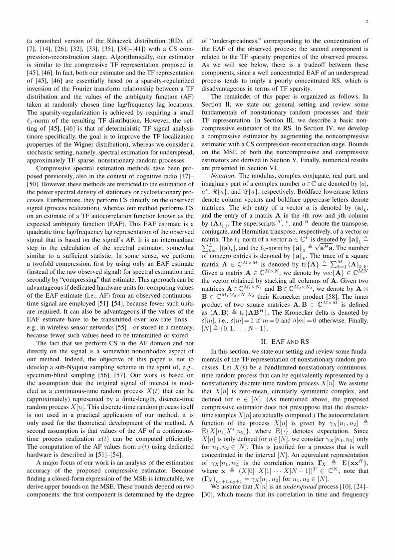
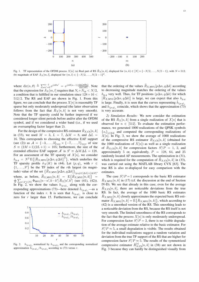
Fig. 1. TF representation of the OFDM process X[n]: (a) Real part of RS RX [n, k], displayed for (n, k) ∈ [N ]×{−N/2, . . . , N/2− 1}, with N= 512;

(b) magnitude of EAF AX [m, l], displayed for (m, l) ∈ {−N/2, . . . , N/2 − 1}2 .

where dir(n, θ) ,∑n−1

n′=0 ejπθn′

= ejπθ(n−1) sin(πθn)sin(πθ) . Note

that the expression for AX [m, l] requires that Ns+Ncp < N/2,

a condition that is fulfilled in our simulation since 128+16 <512/2. The RS and EAF are shown in Fig. 1. From this

figure, we can conclude that the process X [n] is reasonably TF

sparse but only moderately underspread (the latter observation

follows from the fact that RX [n, k] is not very smooth).

Note that the TF sparsity could be further improved if we

considered longer silent periods before and/or after the OFDM

symbol, and if we considered a wider band (i.e., if we used

an oversampling factor larger than 2).

For the design of the compressive RS estimator RX,CS[n, k]in (33), we used M = 3, L = 7, ∆M = 8, and ∆L =16. This corresponds to choosing the effective EAF support

(see (2)) as A = {−3, . . . , 3}512 × {−7, . . . , 7}512, of size

S ≡ (2M +1)(2L+1) = 105; furthermore, the size of the

extended effective EAF support A′ is S′ ≡ ∆M∆L = 128.

For an assessment of the TF sparsity of X [n], we consider

hp,q = N2 E{∣∣RX,MVU[p∆n, q∆k]

∣∣2}, which underlies the

TF sparsity profile σX(K) in (44). Let (p, q)r with r ∈{1, . . . , S′} be the TF index of the rth largest (in magni-

tude) value of the set{RX,MVU[p∆n, q∆k]

}(p,q)∈[∆L]×[∆M ]

,

where, as before, RX,MVU[n, k] = E{RX,MVU[n, k]

}=

1N

∑n′,k′∈[N ]ΦMVU[n−n′, k−k′] RX [n′, k′] (see (41), (42)).

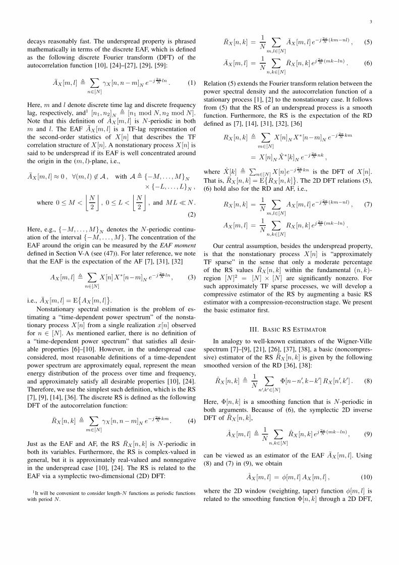
In Fig. 2, we show the values h(p,q)r

along with the cor-

responding approximations (73)—here denoted h(p,q)r—as a

function of the index r. It is seen that h(p,q)r

is close to

zero for r larger than 15. Furthermore, we can conclude

0.2

0.4

0.6

0.8

1

10 20 30 40 50 60 70

h(p,q)r/h(p,q)1

h(p,q)r/h(p,q)1

r

Fig. 2. h(p,q)rnormalized by h(p,q)1

and the corresponding normalized

approximation h(p,q)r/h(p,q)1

according to (73) versus r.

that the ordering of the values RX,MVU[p∆n, q∆k] according

to decreasing magnitude matches the ordering of the values

hp,q very well. Thus, for TF positions (p∆n, q∆k) for which∣∣RX,MVU[p∆n, q∆k]∣∣ is large, we can expect that also hp,q

is large. Finally, it is seen that the curves representing h(p,q)r

and h(p,q)r coincide, which shows that the approximation (73)

is very accurate.

2) Simulation Results: We now consider the estimation

of the RS RX [n, k] from a single realization of X [n] that is

observed for n ∈ [512]. To evaluate the estimation perfor-

mance, we generated 1000 realizations of the QPSK symbols

{si}i∈[64] and computed the corresponding realizations of

X [n]. In Fig. 3, we show the average of 1000 realizations

of the compressive RS estimator RX,CS[n, k] (obtained for

the 1000 realizations of X [n]) as well as a single realization

of RX,CS[n, k] for compression factors S′/P = 1, 2, and

approximately 5 or, equivalently, P = 128, 64, and 25randomly located AF measurements. The optimization in (31),

which is required for the computation of RX,CS[n, k] in (33),

was carried out using the MATLAB library CVX [63]. The

true RS is also re-displayed for easy comparison with the

estimates.

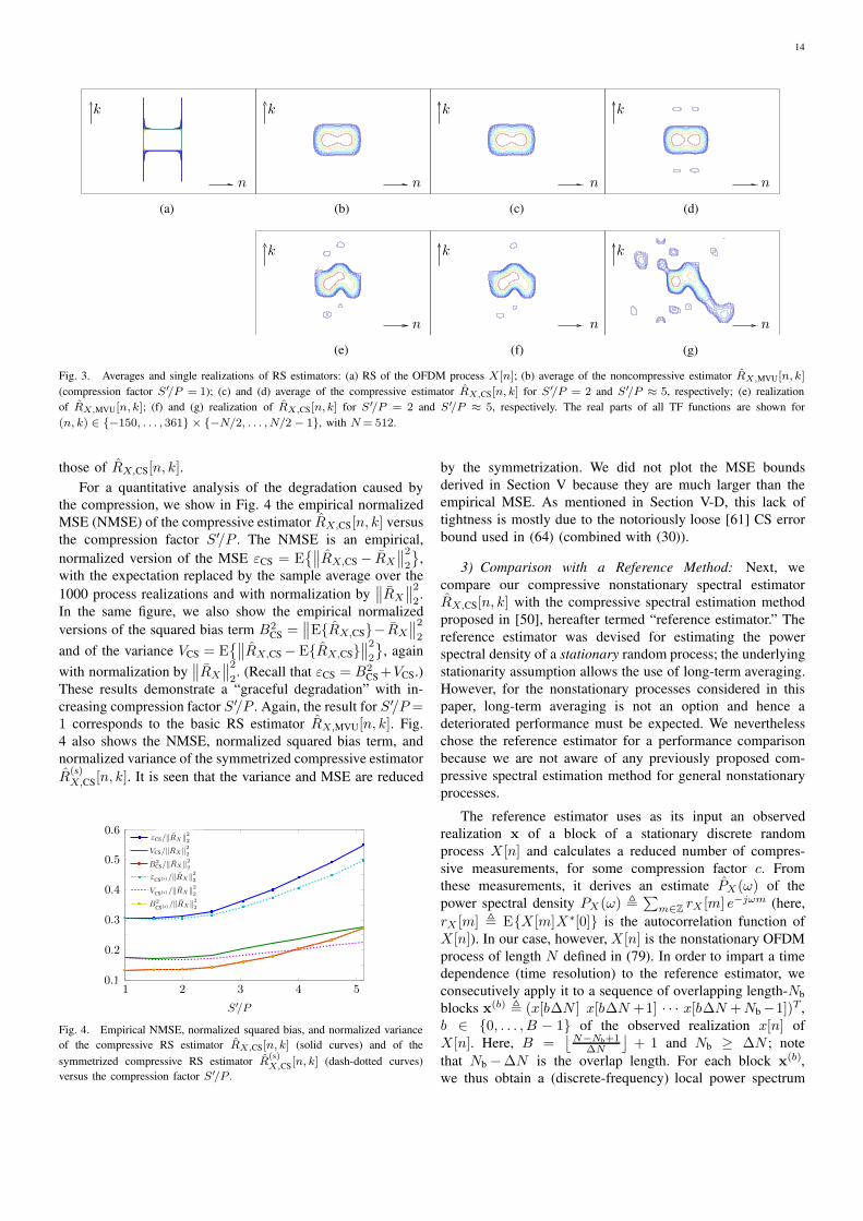
The case S′/P =1 corresponds to the basic RS estimator

RX,MVU[n, k] in (17) (cf. the discussion at the end of Section

IV-D). We see that already in this case, even for the average

RX,CS[n, k], there are noticeable deviations from the true

RS. In fact, the average of the 1000 basic RS estimates

RX,MVU[n, k] closely approximates the expected basic RS esti-

mator RX,MVU[n, k] = E{RX,MVU[n, k]

}, which according to

(42) is a smoothed version of the RS. This smoothing leads to

a noticeable deviation from the RS, because the RS itself is not

very smooth. The limited smoothness of the RS corresponds to

the fact that the process X [n] is only moderately underspread.

For compression factor S′/P = 2, there is no visible degrada-

tion of the average estimate relative to the basic estimator. For

S′/P ≈ 5, a small degradation is visible. The results obtained

for the individual realizations suggest a random variation and

deviation from the true TF support of the RS that are higher for

compression factor S′/P ≈ 5. The results of the symmetrized

compressive estimator R(s)X,CS[n, k] in (38) are not shown in

Fig. 3 because they can hardly be distinguished visually from

14

kk

kkkk

k

n

nnnn

nn

(a) (b) (c) (d)

(e) (f) (g)

Fig. 3. Averages and single realizations of RS estimators: (a) RS of the OFDM process X[n]; (b) average of the noncompressive estimator RX,MVU[n, k]

(compression factor S′/P = 1); (c) and (d) average of the compressive estimator RX,CS[n, k] for S′/P = 2 and S′/P ≈ 5, respectively; (e) realization

of RX,MVU[n, k]; (f) and (g) realization of RX,CS[n, k] for S′/P = 2 and S′/P ≈ 5, respectively. The real parts of all TF functions are shown for

(n, k) ∈ {−150, . . . , 361} × {−N/2, . . . , N/2 − 1}, with N= 512.

those of RX,CS[n, k].

For a quantitative analysis of the degradation caused by

the compression, we show in Fig. 4 the empirical normalized

MSE (NMSE) of the compressive estimator RX,CS[n, k] versus

the compression factor S′/P . The NMSE is an empirical,

normalized version of the MSE εCS = E{∥∥RX,CS − RX

∥∥22

},

with the expectation replaced by the sample average over the

1000 process realizations and with normalization by∥∥RX

∥∥22.

In the same figure, we also show the empirical normalized

versions of the squared bias term B2CS =

∥∥E{RX,CS}− RX∥∥22

and of the variance VCS = E{∥∥RX,CS − E{RX,CS}

∥∥22

}, again

with normalization by∥∥RX

∥∥22. (Recall that εCS = B2

CS+VCS.)

These results demonstrate a “graceful degradation” with in-

creasing compression factor S′/P . Again, the result for S′/P =1 corresponds to the basic RS estimator RX,MVU[n, k]. Fig.

4 also shows the NMSE, normalized squared bias term, and

normalized variance of the symmetrized compressive estimator

R(s)X,CS[n, k]. It is seen that the variance and MSE are reduced

0.1

0.2

0.3

0.4

0.5

0.6εCS/‖RX‖

2

2

B2CS/‖RX‖

2

2

VCS/‖RX‖2

2

εCS(s)/‖RX‖2

2

B2CS(s)/‖RX‖

2

2

VCS(s)/‖RX‖2

2

1 2 3 4 5

S′/P

Fig. 4. Empirical NMSE, normalized squared bias, and normalized variance

of the compressive RS estimator RX,CS[n, k] (solid curves) and of the

symmetrized compressive RS estimator R(s)X,CS

[n, k] (dash-dotted curves)

versus the compression factor S′/P .

by the symmetrization. We did not plot the MSE bounds

derived in Section V because they are much larger than the

empirical MSE. As mentioned in Section V-D, this lack of

tightness is mostly due to the notoriously loose [61] CS error

bound used in (64) (combined with (30)).

3) Comparison with a Reference Method: Next, we

compare our compressive nonstationary spectral estimator

RX,CS[n, k] with the compressive spectral estimation method

proposed in [50], hereafter termed “reference estimator.” The

reference estimator was devised for estimating the power

spectral density of a stationary random process; the underlying

stationarity assumption allows the use of long-term averaging.

However, for the nonstationary processes considered in this

paper, long-term averaging is not an option and hence a

deteriorated performance must be expected. We nevertheless

chose the reference estimator for a performance comparison

because we are not aware of any previously proposed com-

pressive spectral estimation method for general nonstationary

processes.

The reference estimator uses as its input an observed

realization x of a block of a stationary discrete random

process X [n] and calculates a reduced number of compres-

sive measurements, for some compression factor c. From

these measurements, it derives an estimate PX(ω) of the

power spectral density PX(ω) ,∑

m∈ZrX [m] e−jωm (here,

rX [m] , E{X [m]X∗[0]} is the autocorrelation function of

X [n]). In our case, however, X [n] is the nonstationary OFDM

process of length N defined in (79). In order to impart a time

dependence (time resolution) to the reference estimator, we

consecutively apply it to a sequence of overlapping length-Nb

blocks x(b) , (x[b∆N ] x[b∆N +1] · · · x[b∆N +Nb −1])T ,

b ∈ {0, . . . , B − 1} of the observed realization x[n] of

X [n]. Here, B =⌊N−Nb+1

∆N

⌋+ 1 and Nb ≥ ∆N ; note

that Nb −∆N is the overlap length. For each block x(b),

we thus obtain a (discrete-frequency) local power spectrum

15

k

kkk

kkk

nnn

nnnn

(a) (b) (c) (d)

(e) (f) (g)

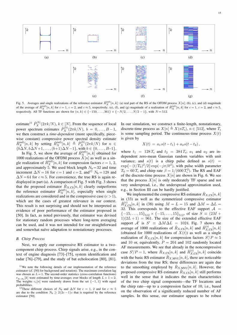
Fig. 5. Averages and single realizations of the reference estimator R(ref)X

[n, k]: (a) real part of the RS of the OFDM process X[n]; (b), (c), and (d) magnitude

of the average of R(ref)X

[n, k] for c= 1, c= 2, and c≈ 5, respectively; (e), (f), and (g) magnitude of a realization of R(ref)X

[n, k] for c= 1, c= 2, and c≈ 5,

respectively. All TF functions are shown for (n, k) ∈ {−150, . . . , 361} × {−N/2, . . . , N/2 − 1}, with N= 512.

estimate11 P(b)X (2πk/N), k ∈ [N ]. From the sequence of local

power spectrum estimates P(b)X (2πk/N), b = 0, . . . , B− 1,

we then construct a time-dependent (more specifically, piece-

wise constant) compressive power spectral density estimate

R(ref)X [n, k] by setting R(ref)

X [n, k] , P(b)X (2πk/N) for n ∈

{b∆N, b∆N+1, . . . , (b+1)∆N−1}, with b ∈ {0, . . . , B−1}.

In Fig. 5, we show the average of R(ref)X [n, k] obtained for

1000 realizations of the OFDM process X [n] as well as a sin-

gle realization of R(ref)X [n, k] for compression factors c= 1, 2,

and approximately 5. We used block length Nb=32 and time

increment ∆N =16 for c=1 and c=2, and12 Nb =128 and

∆N=64 for c≈ 5. For convenience, the true RS is again re-

displayed in part (a). A comparison of Fig. 5 with Fig. 3 shows

that the proposed estimator RX,CS[n, k] clearly outperforms

the reference estimator R(ref)X [n, k], especially when single

realizations are considered and in the compressive case (c >1),

which are the cases of greatest relevance in our context.

This result is not surprising and should not be interpreted as

evidence of poor performance of the estimator proposed in

[50]. In fact, as noted previously, that estimator was devised

for stationary random processes where long-term averaging

can be used, and it was not intended for our straightforward

and somewhat naïve adaptation to nonstationary processes.

B. Chirp Process

Next, we apply our compressive RS estimator to a two-

component chirp process. Chirp signals arise, e.g., in the con-

text of engine diagnosis [73]–[75], system identification and

radar [76]–[79], and the study of bat echolocation [80], [81].

11We note the following details of our implementation of the referenceestimator (cf. [50] for background and notation). The maximum correlation lagwas chosen as L=1. The second-order statistics (cross-correlation functions)ryi,yj [k] were estimated by time-averages over blocks of length L+ 1= 2.

The weights ci[n] were randomly drawn from the set {−1, 1} with equalprobabilities.

12These different choices of Nb and ∆N for c = 1, 2 and for c ≈ 5are due to the condition Nb ≥ 2(2c−1)c that is required by the referenceestimator [50].

In our simulation, we construct a finite-length, nonstationary,

discrete-time process as X [n] , X(nTs), n ∈ [512], where Ts

is some sampling period. The continuous-time process X(t)is given by

X(t) = a1s(t− t1) + a2s(t− t2) ,

where t1 = 128Ts and t2 = 384Ts; a1 and a2 are in-

dependent zero-mean Gaussian random variables with unit

variance; and s(t) is a chirp pulse defined as s(t) =exp

(− (t/T0)

2/2)exp(−jπβt2), with pulse width parameter

T0 = 60Ts and chirp rate β = 1/(600T 2s ). The RS and EAF

of the discrete-time process X [n] are shown in Fig. 6. We see

that the process X [n] is only moderately TF sparse and not

very underspread, i.e., the underspread approximation used,

e.g., in Section III can be hardly justified.

We implemented the compressive RS estimator RX,CS[n, k]in (33) as well as the symmetrized compressive estimator

R(s)X,CS[n, k] in (38) using M = L = 15 and ∆M = ∆L =

32. This corresponds to the effective EAF support A ={−15, . . . , 15}512 × {−15, . . . , 15}512, of size S ≡ (2M +1)(2L +1) = 961. The size of the extended effective EAF

support A′ is S′ ≡ ∆M∆L = 1024. Fig. 7 shows the

average of 1000 realizations of RX,CS[n, k] and R(s)X,CS[n, k]

(obtained for 1000 realizations of X(t)) as well as a single

realization of RX,CS[n, k] for compression factors S′/P ≈ 5and 10 or, equivalently, P = 204 and 102 randomly located

AF measurements. We see that already in the noncompressive

case S′/P = 1, where RX,CS[n, k] and R(s)X,CS[n, k] coincide

with the basic RS estimator RX,MVU[n, k], there are noticeable

deviations from the true RS; these differences are again due

to the smoothing employed by RX,MVU[n, k]. However, the

proposed compressive RS estimator RX,CS[n, k] still performs

well in the sense that it indicates the main characteristics

of the two chirp signal components—the TF locations and

the chirp rate—up to a compression factor of 10, i.e., based

on the observation of a significantly reduced number of AF

samples. In this sense, our estimator appears to be robust

16

(a) (b)

mn

lk

0 100 200 300 400 500 0−100 100−200 200

0 0

−100 −100

100 100

−200 −200

200 200

Fig. 6. TF representation of the two-component chirp process X[n]: (a) Real part of RS RX [n, k], displayed for (n, k) ∈ [N ]× {−N/2, . . . , N/2− 1},

with N= 512; (b) magnitude of EAF AX [m, l], displayed for (m, l) ∈ {−N/2, . . . , N/2− 1}2.

kkk

kk

kkkk

nnn

nn

nnnn

(a) (b) (c) (d)

(e) (f) (g)

(h) (i)

Fig. 7. Averages and single realizations of RS estimators: (a) RS of the chirp process X[n]; (b) average of the noncompressive estimator RX,MVU[n, k]

(compression factor S′/P = 1); (c) and (d) average of the compressive estimator RX,CS[n, k] for S′/P ≈ 5 and 10, respectively; (e) realization of

RX,MVU[n, k]; (f) and (g) realization of RX,CS[n, k] for S′/P ≈ 5 and 10, respectively; (h) and (i) average of the symmetrized compressive estimator

R(s)X,CS

[n, k] for S′/P ≈ 5 and 10, respectively. The real parts of all TF functions are shown for (n, k) ∈ [N ]× {−N/2, . . . , N/2− 1}, with N= 512.

to deviations from the assumed properties of approximate

TF sparsity and underspreadness. More specifically, the main

deviation from the true RS is due to the fact that the oscillatory

structures (inner interference terms [82]) contained in the RS

are suppressed by the smoothing; this result is in fact desirable

in most applications. It is furthermore seen that the average

results of the symmetrized estimator R(s)X,CS[n, k] are similar

to those of RX,CS[n, k].

VII. CONCLUSION

For estimating a time-dependent spectrum of a nonstation-

ary random process, long-term averaging cannot be used as

this would smear out the time-dependence of the spectrum.

However, if the spectrum as a function of time and frequency

is sufficiently smooth, which amounts to an underspread as-

sumption, a local TF smoothing can be used. In particular, the

RS of an underspread nonstationary process can be estimated

by a local smoothing of a TF distribution known as the RD.

In this paper, we have considered the practically relevant

case of underspread processes that are approximately TF

sparse in the sense that only a moderate percentage of the RS

values are significantly nonzero. For such processes, we have

proposed a “compressive” RS estimator that exploits the TF

sparsity structure for a significant reduction of the number of

measurements required for good estimation performance. The

measurements are values of the AF of the observed signal

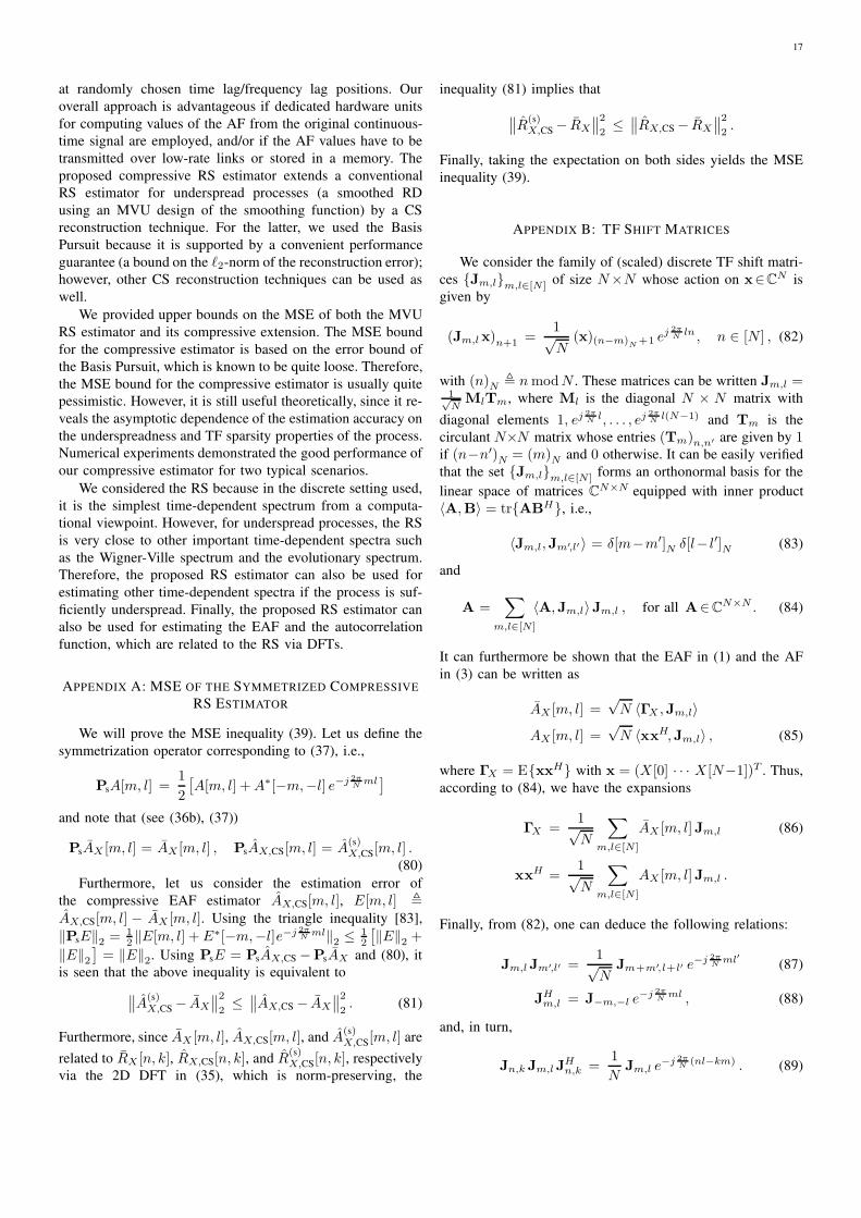
17

at randomly chosen time lag/frequency lag positions. Our

overall approach is advantageous if dedicated hardware units

for computing values of the AF from the original continuous-

time signal are employed, and/or if the AF values have to be

transmitted over low-rate links or stored in a memory. The

proposed compressive RS estimator extends a conventional

RS estimator for underspread processes (a smoothed RD

using an MVU design of the smoothing function) by a CS

reconstruction technique. For the latter, we used the Basis

Pursuit because it is supported by a convenient performance

guarantee (a bound on the ℓ2-norm of the reconstruction error);

however, other CS reconstruction techniques can be used as

well.

We provided upper bounds on the MSE of both the MVU

RS estimator and its compressive extension. The MSE bound

for the compressive estimator is based on the error bound of

the Basis Pursuit, which is known to be quite loose. Therefore,

the MSE bound for the compressive estimator is usually quite

pessimistic. However, it is still useful theoretically, since it re-

veals the asymptotic dependence of the estimation accuracy on

the underspreadness and TF sparsity properties of the process.

Numerical experiments demonstrated the good performance of

our compressive estimator for two typical scenarios.

We considered the RS because in the discrete setting used,

it is the simplest time-dependent spectrum from a computa-

tional viewpoint. However, for underspread processes, the RS

is very close to other important time-dependent spectra such

as the Wigner-Ville spectrum and the evolutionary spectrum.

Therefore, the proposed RS estimator can also be used for

estimating other time-dependent spectra if the process is suf-

ficiently underspread. Finally, the proposed RS estimator can

also be used for estimating the EAF and the autocorrelation

function, which are related to the RS via DFTs.

APPENDIX A: MSE OF THE SYMMETRIZED COMPRESSIVE

RS ESTIMATOR

We will prove the MSE inequality (39). Let us define the

symmetrization operator corresponding to (37), i.e.,

PsA[m, l] =1

2

[A[m, l] +A∗[−m,−l] e−j 2π

Nml

]

and note that (see (36b), (37))

PsAX [m, l] = AX [m, l] , PsAX,CS[m, l] = A(s)X,CS[m, l] .

(80)

Furthermore, let us consider the estimation error of

the compressive EAF estimator AX,CS[m, l], E[m, l] ,AX,CS[m, l] − AX [m, l]. Using the triangle inequality [83],

‖PsE‖2 = 12 ‖E[m, l] + E∗[−m,−l]e−j 2π

Nml‖2 ≤ 1

2

[‖E‖2 +

‖E‖2]= ‖E‖2. Using PsE = PsAX,CS −PsAX and (80), it

is seen that the above inequality is equivalent to

∥∥A(s)X,CS − AX

∥∥22≤

∥∥AX,CS − AX∥∥22. (81)

Furthermore, since AX [m, l], AX,CS[m, l], and A(s)X,CS[m, l] are

related to RX [n, k], RX,CS[n, k], and R(s)X,CS[n, k], respectively

via the 2D DFT in (35), which is norm-preserving, the

inequality (81) implies that

∥∥R(s)X,CS − RX

∥∥22≤

∥∥RX,CS − RX∥∥22.

Finally, taking the expectation on both sides yields the MSE

inequality (39).

APPENDIX B: TF SHIFT MATRICES

We consider the family of (scaled) discrete TF shift matri-

ces {Jm,l}m,l∈[N ] of size N×N whose action on x∈CN is

given by

(Jm,lx)n+1 =1√N

(x)(n−m)N+1 e

j 2πNln , n ∈ [N ] , (82)

with (n)N , nmodN . These matrices can be written Jm,l =1√NMlTm, where Ml is the diagonal N × N matrix with

diagonal elements 1, ej2πNl, . . . , ej

2πNl(N−1) and Tm is the

circulant N×N matrix whose entries (Tm)n,n′ are given by 1if (n−n′)N = (m)N and 0 otherwise. It can be easily verified

that the set {Jm,l}m,l∈[N ] forms an orthonormal basis for the

linear space of matrices CN×N equipped with inner product

〈A,B〉 = tr{ABH}, i.e.,

〈Jm,l,Jm′,l′〉 = δ[m−m′]N δ[l− l′]N (83)

and

A =∑

m,l∈[N ]

〈A,Jm,l〉Jm,l , for all A∈CN×N . (84)

It can furthermore be shown that the EAF in (1) and the AF

in (3) can be written as

AX [m, l] =√N 〈ΓX ,Jm,l〉

AX [m, l] =√N 〈xxH,Jm,l〉 , (85)

where ΓX = E{xxH} with x = (X [0] · · · X [N−1])T . Thus,

according to (84), we have the expansions

ΓX =1√N

∑

m,l∈[N ]

AX [m, l]Jm,l (86)

xxH =

1√N

∑

m,l∈[N ]

AX [m, l]Jm,l .

Finally, from (82), one can deduce the following relations:

Jm,lJm′,l′ =1√N

Jm+m′,l+l′ e−j 2π

Nml′ (87)

JHm,l = J−m,−l e

−j 2πNml , (88)

and, in turn,

Jn,k Jm,lJHn,k =

1

NJm,l e

−j 2πN

(nl−km) . (89)

18

APPENDIX C: DERIVATION OF EXPRESSIONS (58) AND (59)

We will derive (58) and (59) from (57). Our derivation will

be based on expansions of C(R)n,k and C

(I)n,k into the TF shift

matrices Jm,l. Using (55), (50), and (88), we have

C(R)n,k

(55),(50)=

1

2√N

[M∑

m=−M

L∑

l=−Le−j

2πN

(km−nl)JHm,l

+

M∑

m=−M

L∑

l=−Lej

2πN

(km−nl)Jm,l

]

(88)=

1

2√N

[M∑

m=−M

L∑

l=−Le−j

2πN

(km−nl)J−m,−l e

−j 2πNml

+

M∑

m=−M

L∑

l=−Lej

2πN

(km−nl)Jm,l

]

=1

2√N

M∑

m=−M

L∑

l=−Lej

2πN

(km−nl) (e−j 2πNml + 1

)Jm,l

=∑

m,l∈[N ]

ej2πN

(km−nl) c(R)m,l Jm,l , (90)

with

c(R)m,l ,

1

2√N

IA[m, l](e−j

2πNml +1

). (91)

In a similar way, we obtain from (55)

C(I)n,k =

∑

m,l∈[N ]

ej2πN

(km−nl) c(I)m,l Jm,l , (92)

with

c(I)m,l ,

1

2j√N

IA[m, l](e−j

2πNml−1

). (93)

The first term in (57) can then be written as∑

n,k∈[N ]

tr{C

(R)n,kΓXC

(R)n,kΓX

}= tr

{DΓX

}= tr

{DΓ

HX

},

(94)with

D ,∑

n,k∈[N ]

C(R)n,kΓXC

(R)n,k

=∑

n,k∈[N ]

C(R)n,kΓXC

(R)Hn,k

(90)=

∑

m,l,m′,l′∈[N ]

c(R)m,l c

(R)∗m′,l′

×[

∑

n,k∈[N ]

ej2πN

[k(m−m′)−n(l−l′)]]

︸ ︷︷ ︸N2 δ[m−m′]

Nδ[l−l′]

N

Jm,lΓXJHm′,l′

= N2∑

m,l∈[N ]

∣∣c(R)m,l

∣∣2 Jm,lΓXJHm,l

(86)= N

√N

∑

m,l,m′,l′∈[N ]

∣∣c(R)m,l

∣∣2 AX [m′, l′]Jm,lJm′,l′JHm,l

(89)=

√N

∑

m,l,m′,l′∈[N ]

∣∣c(R)m,l

∣∣2 AX [m′, l′]Jm′,l′

× e−j2πN

(ml′−lm′) (95)

and

ΓHX

(86)=

1√N

∑

m,l∈[N ]

A∗X [m, l]JHm,l . (96)

Inserting (95) and (96) into (94) then yields

∑

n,k∈[N ]

tr{C

(R)n,kΓXC

(R)n,kΓX

}

= tr

{∑

m,l,m′,l′,m′′,l′′∈[N ]

∣∣c(R)m,l

∣∣2 AX [m′, l′]Jm′,l′

× e−j2πN

(ml′−lm′) A∗X [m′′, l′′]JHm′′,l′′

}

=∑

m,l,m′,l′,m′′,l′′∈[N ]

∣∣c(R)m,l

∣∣2 AX [m′, l′]A∗X [m′′, l′′]

× e−j2πN

(ml′−lm′) tr{Jm′,l′J

Hm′′,l′′

}︸ ︷︷ ︸

〈Jm′,l′ ,Jm′′,l′′ 〉(83)= δ[m′−m′′]N δ[l

′−l′′]N

=∑

m,l,m′,l′∈[N ]

∣∣c(R)m,l

∣∣2 ∣∣AX [m′, l′]∣∣2 e−j 2π

N(ml′−lm′)

=∑

m,l,m′,l′∈[N ]

∣∣c(R)m,l

∣∣2 ∣∣AX [m′, l′]∣∣2 ej 2π

N(ml′−lm′) , (97)

where the symmetry relation (36b) has been used in the last

step.

In a similar manner, using (92), we obtain for the second

term in (57)∑

n,k∈[N ]

tr{C

(I)n,kΓXC

(I)n,kΓX

}

=∑

m,l,m′,l′∈[N ]

∣∣c(I)m,l

∣∣2 ∣∣AX [m′, l′]∣∣2 ej 2π

N(ml′−lm′) . (98)

Inserting (97) and (98) into (57) then gives (58):

V =∑

m,l,m′,l′∈[N ]

∣∣c(R)m,l

∣∣2 ∣∣AX [m′, l′]∣∣2 ej 2π

N(ml′−lm′)

+∑

m,l,m′,l′∈[N ]

∣∣c(I)m,l

∣∣2 ∣∣AX [m′, l′]∣∣2 ej 2π

N(ml′−lm′)

=∑

m′,l′∈[N ]

∣∣AX [m′, l′]∣∣2 χ[m′, l′] ,

with

χ[m, l] ,∑

m′,l′∈[N ]

(∣∣c(R)m′,l′

∣∣2 +∣∣c(I)m′,l′

∣∣2) ej 2πN

(m′l−l′m) . (99)

Using (91) and (93), we have

∣∣c(R)m,l

∣∣2 +∣∣c(I)m,l

∣∣2

=1

NIA[m, l]

[∣∣∣∣e−j

2πNml + 1

2

∣∣∣∣2

+

∣∣∣∣e−j

2πNml − 1

2j

∣∣∣∣2]

=1

NIA[m, l]

[cos2

( πNml

)+ sin2

( πNml

)]

19

=1

NIA[m, l] .

Inserting this into (99) yields (59).

APPENDIX D: DERIVATION OF EXPRESSION (73)

We will derive (73) from (72).

1) Expansions of T(R)p,q and T

(I)p,q: Our derivation will be

based on the underspread assumption and on expansions of

T(R)p,q and T

(I)p,q into the TF shift matrices Jm,l. Inserting (70)

into the definition of T(R)p,q in (71) yields

T(R)p,q =

√N

2

[M∑

m=−M

L∑

l=−Le−j2π

(qm∆M

− pl∆L

)JHm,l

+

M∑

m=−M

L∑

l=−Lej2π

(qm∆M

− pl∆L

)Jm,l

]

(88)=

√N

2

[M∑

m=−M

L∑

l=−Le−j2π

(qm∆M

− pl∆L

)J−m,−l e

−j 2πNml

+M∑

m=−M

L∑

l=−Lej2π

(qm∆M

− pl∆L

)Jm,l

]

=

√N

2

M∑

m=−M

L∑

l=−Lej2π

(qm∆M

− pl∆L

)(e−j

2πNml +1

)Jm,l

=∑

m,l∈[N ]

ej2π(

qm∆M

− pl∆L

)t(R)m,l Jm,l , (100)

with

t(R)m,l =

√N

2IA[m, l]

(e−j

2πNml +1

). (101)

In a similar manner, we obtain the expansion

T(I)p,q =

∑

m,l∈[N ]

ej2π(

qm∆M

− pl∆L

)t(I)m,l Jm,l , (102)

with

t(I)m,l =

√N

2jIA[m, l]

(e−j

2πNml− 1

). (103)

For an underspread process X [n], the effective EAF sup-

port A ≡ {−M, . . . ,M}N ×{−L, . . . , L}N is a small region

about the origin of the (m, l) plane (plus its periodically

continued replicas, which are irrelevant to our argument and

will hence be disregarded). Looking at the expressions of

t(R)m,l and t

(I)m,l in (101) and (103), we can then conclude from

the presence of the factor IA[m, l] that t(R)m,l and t

(I)m,l can be

nonzero only for |ml| ≪ N . This means that in (101) and

(103), we can approximate e−j2πNml by 1, yielding

t(R)m,l ≈

√N IA[m, l] (104)

t(I)m,l ≈ 0 . (105)

Using (105) in (102) yields

T(I)p,q ≈ 0 , (106)

and thus (72) approximately simplifies to

hp,q ≈ tr{T

(R)p,qΓXT

(R)p,qΓX

}+

∣∣tr{ΓXTHp,q}

∣∣2 . (107)

2) First term in (107): We will now develop the two terms

on the right-hand side of (107). The first term can be written

as

tr{T

(R)p,qΓXT

(R)p,qΓX

}=

⟨T

(R)p,qΓX ,

(T

(R)p,qΓX

)H⟩. (108)

In order to find an approximation for this inner product, we

use the following general result for the product C = AB of

two N×N matrices A and B. The matrices A, B, and C

can be expanded into the orthonormal basis {Jm,l}m,l∈[N ],

with respective expansion coefficients am,l, bm,l, and cm,l,e.g., A =

∑m,l∈[N ] am,l Jm,l. Then the cm,l are related to the

am,l and bm,l by the “twisted convolution” [24], [29], [84],

[85]

cm,l =1√N

∑

m′,l′∈[N ]

am′,l′ bm−m′,l−l′ e−j 2π

Nm′(l−l′) . (109)

This expression can be verified using (87). Let us apply it to

the matrix product T(R)p,qΓX . We have the expansion

T(R)p,qΓX =

∑

m,l∈[N ]

dp,q;m,l Jm,l . (110)

The expansion coefficients of T(R)p,q are ej2π

(qm∆M

− pl∆L

)t(R)m,l

(see (100)); those of ΓX are 1√NAX [m, l] (see (86)). Inserting

these expressions into (109) yields

dp,q;m,l =1√N

∑

m′,l′∈[N ]

[ej2π

(qm′

∆M− pl′

∆L

)t(R)m′,l′

]

×[

1√NAX [m−m′, l− l′]

]e−j

2πNm′(l−l′)

≈ 1√N

∑

m′,l′∈[N ]

ej2π(

qm′

∆M− pl′

∆L

)IA[m

′, l′]

× AX [m−m′, l− l′] e−j 2πNm′(l−l′) , (111)

where the approximate expression (104) was used in the last

step. For an underspread process, because of the support of

IA[m, l] and the effective support of AX [m, l], the terms in the

sum (111) are significantly nonzero only for |m′(l− l′)| ≪ N .

We can thus use the approximation e−j2πNm′(l−l′) ≈ 1, which

yields

dp,q;m,l ≈ 1√N

∑

m′,l′∈[N ]

IA[m′, l′] AX [m−m′, l− l′]

× ej2π(

qm′

∆M− pl′

∆L

). (112)

Next, we consider

(T

(R)p,qΓX

)H (110)=

∑

m,l∈[N ]

d∗p,q;m,l JHm,l

(88)=

∑

m,l∈[N ]

d∗p,q;m,l J−m,−l e−j 2π

Nml

=∑

m,l∈[N ]

d∗p,q;−m,−l Jm,l e−j 2π

Nml , (113)

where the N -periodicity of dp,q;m,l with respect to m and lwas used in the last step. For an underspread process, again

20

because of the support of IA[m, l] and the effective support of

AX [m, l], it follows from (112) that the coefficients dp,q;m,lare significantly nonzero only for |ml| ≪ N . Hence, we can

set e−j2πNml ≈ 1 in (113), which gives

(T

(R)p,qΓX

)H ≈∑

m,l∈[N ]

d∗p,q;−m,−l Jm,l . (114)

In a similar way, we obtain from (36b) the following approx-

imation:

A∗X [−m,−l] ≈ AX [m, l] , for |ml| ≪N . (115)

We now insert (110) and (114) into (108), and obtain

tr{T

(R)p,qΓXT

(R)p,qΓX

}

≈⟨

∑

m,l∈[N ]

dp,q;m,l Jm,l ,∑

m′,l′∈[N ]

d∗p,q;−m′,−l′ Jm′,l′

⟩

(83)=

∑

m,l∈[N ]

dp,q;m,l dp,q;−m,−l . (116)

From the underspread approximations (112) and (115), it

readily follows that dp,q;−m,−l ≈ d∗p,q;m,l. Indeed,

dp,q;−m,−l(112)≈ 1√

N

∑

m′,l′∈[N ]

IA[m′, l′] AX [−m−m′,−l− l′]

× ej2π(

qm′

∆M− pl′

∆L

)

(115)≈ 1√N

∑

m′,l′∈[N ]

IA[m′, l′] A∗

X [m+m′, l+ l′]

× ej2π(

qm′

∆M− pl′

∆L

)

(∗)=

1√N

M∑

m′=−M

L∑

l′=−LA∗X [m+m′, l+ l′]

× ej2π(

qm′

∆M− pl′

∆L

)

=1√N

M∑

m′=−M

L∑

l′=−LA∗X [m−m′, l− l′]

× e−j2π(

qm′

∆M− pl′

∆L

)

(∗)=

1√N

∑

m′,l′∈[N ]

IA[m′, l′] A∗

X [m−m′, l− l′]

× e−j2π(

qm′

∆M− pl′

∆L

)

(112)≈ d∗p,q;m,l , (117)

where the periodicity of the summand with respect to m′ and

l′ has been exploited in the steps labeled with (∗). Using (117)

in (116) then gives

tr{T

(R)p,qΓXT

(R)p,qΓX

}≈

∑

m,l∈[N ]

|dp,q;m,l|2 . (118)

3) Second term in (107): Next, we consider the second

term on the right-hand side of (107). We have

tr{ΓXTHp,q}

(71)= tr

{ΓXT

(R)p,q

}+ j tr

{ΓXT

(I)p,q

}

(106)≈ tr{ΓXT

(R)p,q

}

= tr{T

(R)p,qΓX

}. (119)

Using J0,0 =1√NI, where I denotes the N×N identity matrix,

we obtain further

tr{ΓXTHp,q}

(119)≈ tr{T

(R)p,qΓXI

}

=√N tr

{T

(R)p,qΓXJ

H0,0

}

=√N

⟨T

(R)p,qΓX , J0,0

⟩

(110)=

√N

⟨∑

m,l∈[N ]

dp,q;m,l Jm,l ,J0,0

⟩

(83)=

√N dp,q;0,0 . (120)

4) Approximation of hp,q: Inserting (118) and (120) into

(107), we obtain the following approximation of hp,q:

hp,q ≈∑

m,l∈[N ]

|dp,q;m,l|2 + N |dp,q;0,0|2 .

This can be expressed as

hp,q ≈∑

n,k∈[N ]

|dp,q;n,k|2 + N

∣∣∣∣∣1

N

∑

n,k∈[N ]

dp,q;n,k

∣∣∣∣∣

2

, (121)

where dp,q;n,k is the 2D DFT of dp,q;m,l with respect to (m, l).We have

dp,q;n,k

=1

N

∑

m,l∈[N ]

dp,q;m,l e−j 2π

N(km−nl)

(112)≈ 1√N

∑

m′,l′∈[N ]

IA[m′, l′]

[1

N

∑

m,l∈[N ]

AX [m−m′, l− l′]

× e−j2πN

(km−nl)]ej2π

(qm′

∆M− pl′

∆L

)

(5)=

1√N

∑

m′,l′∈[N ]

IA[m′, l′] RX [n, k]

× e−j2πN

(km′−nl′) ej2π(

qm′

∆M− pl′

∆L

)

=1√NRX [n, k]

∑

m′,l′∈[N ]

IA[m′, l′]

× e−j2πN

[(k− N

∆Mq

)m′−

(n− N

∆Lp

)l′]

(43)=

√N RX [n, k] ΦMVU[n− p∆n, k− q∆k] , (122)

where, as before, ∆n = N/∆L and ∆k = N/∆M . Finally,

inserting (122) into (121) yields (73).

ACKNOWLEDGMENT

The authors would like to thank the anonymous reviewers

for numerous helpful comments, which have led to improve-

ments of this paper.

REFERENCES

[1] S. M. Kay, Modern Spectral Estimation. Englewood Cliffs (NJ): Prentice

Hall, 1988.

[2] P. Stoica and R. Moses, Introduction to Spectral Analysis. Englewood

Cliffs (NJ): Prentice Hall, 1997.

[3] S. Haykin, “Cognitive radio: Brain-empowered wireless communica-

tion,” IEEE J. Sel. Areas Comm., vol. 23, pp. 201–220, Feb. 2005.

21

[4] D. Cabric, I. O’Donnell, M.-W. Chen, and R. Brodersen, “Spectrum

sharing radios,” IEEE Circuits and Systems Magazine, vol. 6, no. 2,

pp. 30–45, 2006.

[5] A. Sahai, S. Mishra, R. Tandra, and K. Woyach, “Cognitive radios

for spectrum sharing [applications corner],” IEEE Signal ProcessingMagazine, vol. 26, pp. 140–145, Jan. 2009.

[6] R. M. Loynes, “On the concept of the spectrum for non-stationary

processes,” J. Roy. Stat. Soc. Ser. B, vol. 30, no. 1, pp. 1–30, 1968.

[7] P. Flandrin, Time-Frequency/Time-Scale Analysis. San Diego (CA):

Academic Press, 1999.

[8] W. Martin and P. Flandrin, “Wigner-Ville spectral analysis of nonstation-

ary processes,” IEEE Trans. Acoust., Speech, Signal Processing, vol. 33,

pp. 1461–1470, Dec. 1985.

[9] P. Flandrin and W. Martin, “The Wigner-Ville spectrum of nonstationary

random signals,” in The Wigner Distribution — Theory and Applicationsin Signal Processing (W. Mecklenbräuker and F. Hlawatsch, eds.),

pp. 211–267, Amsterdam (The Netherlands): Elsevier, 1997.

[10] G. Matz and F. Hlawatsch, “Nonstationary spectral analysis based

on time-frequency operator symbols and underspread approximations,”

IEEE Trans. Inf. Theory, vol. 52, pp. 1067–1086, March 2006.

[11] C. H. Page, “Instantaneous power spectra,” J. Appl. Phys., vol. 23,

pp. 103–106, Jan. 1952.

[12] M. J. Levin, “Instantaneous spectra and ambiguity functions,” IEEETrans. Inf. Theory, vol. 10, pp. 95–97, Jan. 1964.

[13] M. B. Priestley, “Evolutionary spectra and non-stationary processes,” J.Roy. Stat. Soc. Ser. B, vol. 27, no. 2, pp. 204–237, 1965.

[14] A. W. Rihaczek, “Signal energy distribution in time and frequency,”

IEEE Trans. Inf. Theory, vol. 14, pp. 369–374, May 1968.

[15] W. D. Mark, “Spectral analysis of the convolution and filtering of non-

stationary stochastic processes,” J. Sound Vib., vol. 11, no. 1, pp. 19–63,

1970.

[16] M. B. Priestley, “Some notes on the physical interpretation of spectra of

nonstationary stochastic processes,” J. Sound Vib., vol. 17, pp. 51–54,

1971.

[17] D. Tjøstheim, “Spectral generating operators for non-stationary pro-

cesses,” Adv. Appl. Prob., vol. 8, pp. 831–846, 1976.

[18] G. Mélard, “Propriétés du spectre évolutif d’un processus non-

stationnaire,” Ann. Inst. H. Poincaré B, vol. XIV, no. 4, pp. 411–424,

1978.

[19] O. D. Grace, “Instantaneous power spectra,” J. Acoust. Soc. Amer.,vol. 69, no. 1, pp. 191–198, 1981.

[20] G. Mélard and A. de Schutter-Herteleer, “Contributions to evolutionary

spectral theory,” J. Roy. Stat. Soc. Ser. B, vol. 10, pp. 41–63, 1989.

[21] P. Flandrin, “Time-dependent spectra for nonstationary stochastic pro-

cesses,” in Time and Frequency Representation of Signals and Systems(G. Longo and B. Picinbono, eds.), pp. 69–124, Vienna, Austria:

Springer, 1989.

[22] C. S. Detka and A. El-Jaroudi, “The transitory evolutionary spectrum,”

in Proc. IEEE ICASSP-94, (Adelaide, Australia), pp. 289–292, April

1994.

[23] G. Matz, F. Hlawatsch, and W. Kozek, “Generalized evolutionary spec-

tral analysis and the Weyl spectrum of nonstationary random processes,”

IEEE Trans. Signal Processing, vol. 45, pp. 1520–1534, June 1997.

[24] G. Matz, A time-frequency calculus for time-varying systems and non-stationary processes with applications. PhD thesis, Vienna University

of Technology, Nov. 2000.

[25] G. Matz and F. Hlawatsch, “Time-varying power spectra of nonstationary

random processes,” in Time-Frequency Signal Analysis and Processing:A Comprehensive Reference (B. Boashash, ed.), ch. 9.4, pp. 400–409,

Oxford (UK): Elsevier, 2003.

[26] G. Matz and F. Hlawatsch, “Time-frequency methods for non-stationary

statistical signal processing,” in Time-Frequency Analysis: Concepts andMethods (F. Hlawatsch and F. Auger, eds.), pp. 279–320, London, UK:

ISTE/Wiley, 2008.

[27] W. Kozek, F. Hlawatsch, H. Kirchauer, and U. Trautwein, “Correla-

tive time-frequency analysis and classification of nonstationary random

processes,” in Proc. IEEE-SP Int. Sympos. Time-Frequency Time-ScaleAnalysis, (Philadelphia, PA), pp. 417–420, Oct. 1994.

[28] W. Kozek, “On the underspread/overspread classification of nonsta-

tionary random processes,” in Proc. Int. Conf. Industrial and Applied

Mathematics (K. Kirchgässner, O. Mahrenholtz, and R. Mennicken,

eds.), vol. 3 of Mathematical Research, (Berlin, Germany), pp. 63–66,

Akademieverlag, 1996.

[29] W. Kozek, Matched Weyl-Heisenberg expansions of nonstationary envi-ronments. PhD thesis, Vienna University of Technology, March 1997.

[30] W. Kozek, “Adaptation of Weyl-Heisenberg frames to underspread envi-

ronments,” in Gabor Analysis and Algorithms: Theory and Applications(H. G. Feichtinger and T. Strohmer, eds.), ch. 10, pp. 323–352, Boston

(MA): Birkhäuser, 1998.

[31] L. Cohen, Time-Frequency Analysis. Englewood Cliffs (NJ): Prentice

Hall, 1995.

[32] F. Hlawatsch and G. F. Boudreaux-Bartels, “Linear and quadratic time-

frequency signal representations,” IEEE Signal Processing Magazine,

vol. 9, pp. 21–67, April 1992.

[33] A. M. Sayeed and D. L. Jones, “Optimal kernels for nonstationary

spectral estimation,” IEEE Trans. Signal Processing, vol. 43, pp. 478–

491, Feb. 1995.

[34] L. L. Scharf, B. Friedlander, P. Flandrin, and A. Hanssen, “The Hilbert

space geometry of the stochastic Rihaczek distribution,” in Proc. 35thAsilomar Conf. Sig., Sys., Comput., (Pacific Grove, CA), pp. 720–725,

Nov. 2001.

[35] L. L. Scharf, B. Friedlander, and D. J. Thomson, “Covariant estimators

of time-frequency descriptors for nonstationary random processes,” in

Proc. 32nd Asilomar Conf. Sig., Sys., Comput., (Pacific Grove, CA),

pp. 808–811, Nov. 1998.

[36] L. L. Scharf, P. J. Schreier, and A. Hanssen, “The Hilbert space geometry

of the Rihaczek distribution for stochastic analytic signals,” IEEE SignalProcessing Letters, vol. 12, pp. 297–300, April 2005.

[37] M. G. Amin, “Time-frequency spectrum analysis and estimation for

non-stationary random processes,” in Time-Frequency Signal Analysis:Methods and Applications (B. Boashash, ed.), pp. 208–232, Melbourne,

Australia: Longman Cheshire, 1992.

[38] W. Kozek and K. Riedel, “Quadratic time-varying spectral estimation for

underspread processes,” in Proc. IEEE-SP Int. Sympos. Time-FrequencyTime-Scale Analysis, (Philadelphia, PA), pp. 460–463, Oct. 1994.

[39] M. Bayram and R. G. Baraniuk, “Multiple window time-frequency

analysis,” in Proc. IEEE-SP Int. Sympos. Time-Frequency Time-ScaleAnalysis, (Paris, France), pp. 173–176, June 1996.

[40] M. Bayram and R. G. Baraniuk, “Multiple window time-varying spec-

trum estimation,” in Nonlinear and Nonstationary Signal Processing(W. Fitzgerald, R. Smith, A. Walden, and P. Young, eds.), pp. 292–316,

Cambridge, UK: Cambridge Univ. Press, 2000.

[41] F. Cakrak and P. J. Loughlin, “Multiple window time-varying spectral

analysis,” IEEE Trans. Signal Processing, vol. 49, pp. 448–453, Feb.

2001.

[42] A. Jung, G. Tauböck, and F. Hlawatsch, “Compressive nonstationary

spectral estimation using parsimonious random sampling of the ambi-

guity function,” in Proc. IEEE-SSP 2009, (Cardiff, Wales, UK), pp. 642–

645, Aug.–Sep. 2009.

[43] D. L. Donoho, “Compressed sensing,” IEEE Trans. Inf. Theory, vol. 52,

pp. 1289–1306, April 2006.

[44] E. J. Candès, J. Romberg, and T. Tao, “Stable signal recovery from

incomplete and inaccurate measurements,” Comm. Pure Appl. Math.,vol. 59, pp. 1207–1223, Aug. 2006.

[45] P. Borgnat and P. Flandrin, “Time-frequency localization from sparsity

constraints,” in Proc. IEEE ICASSP-2008, (Las Vegas, NV), pp. 3785–

3788, Apr. 2008.

[46] P. Flandrin and P. Borgnat, “Time-frequency energy distributions meet

compressed sensing,” IEEE Trans. Signal Processing, vol. 58, pp. 2974–

2982, June 2010.

[47] Z. Tian, “Compressed wideband sensing in cooperative cognitive radio

networks,” in Proc. IEEE GLOBECOM 2008, (New Orleans, LA), pp. 1–

5, Dec. 2008.

[48] Y. Polo, Y. Wang, A. Pandharipande, and G. Leus, “Compressive wide-

band spectrum sensing,” in Proc. IEEE ICASSP-2009, (Taipei, Taiwan),

pp. 2337–2340, Apr. 2009.

[49] Z. Tian, Y. Tafesse, and B. Sadler, “Cyclic feature detection with sub-

Nyquist sampling for wideband spectrum sensing,” IEEE J. Sel. TopicsSig. Proc., vol. 6, pp. 58–69, Feb. 2012.

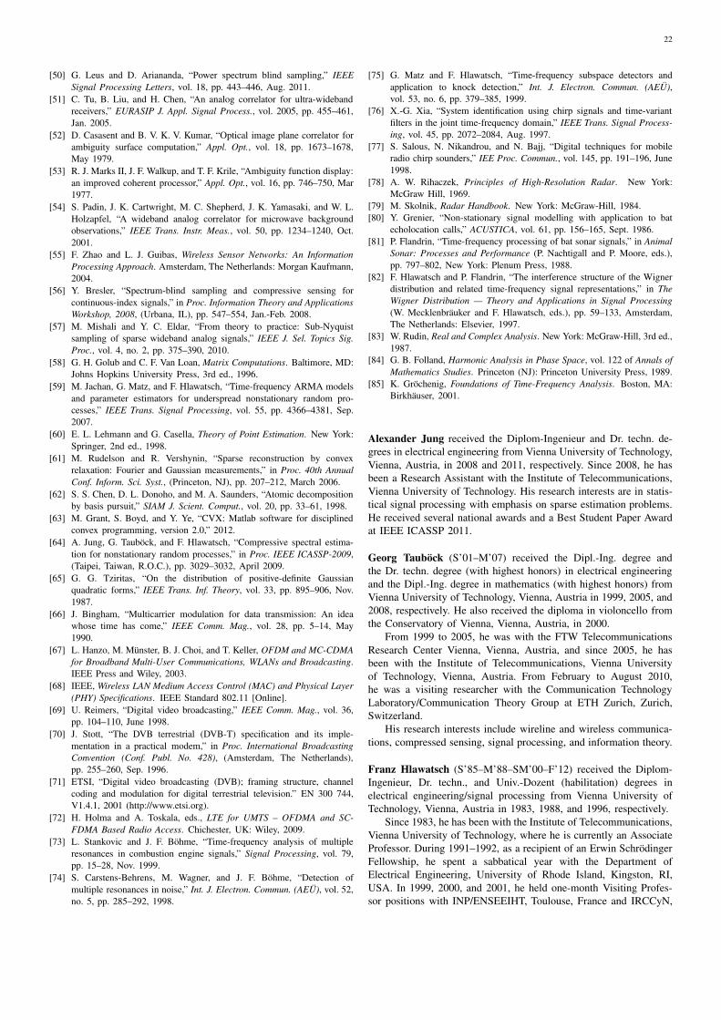
22

[50] G. Leus and D. Ariananda, “Power spectrum blind sampling,” IEEESignal Processing Letters, vol. 18, pp. 443–446, Aug. 2011.

[51] C. Tu, B. Liu, and H. Chen, “An analog correlator for ultra-wideband

receivers,” EURASIP J. Appl. Signal Process., vol. 2005, pp. 455–461,

Jan. 2005.

[52] D. Casasent and B. V. K. V. Kumar, “Optical image plane correlator for

ambiguity surface computation,” Appl. Opt., vol. 18, pp. 1673–1678,

May 1979.

[53] R. J. Marks II, J. F. Walkup, and T. F. Krile, “Ambiguity function display:

an improved coherent processor,” Appl. Opt., vol. 16, pp. 746–750, Mar

1977.

[54] S. Padin, J. K. Cartwright, M. C. Shepherd, J. K. Yamasaki, and W. L.

Holzapfel, “A wideband analog correlator for microwave background

observations,” IEEE Trans. Instr. Meas., vol. 50, pp. 1234–1240, Oct.

2001.

[55] F. Zhao and L. J. Guibas, Wireless Sensor Networks: An InformationProcessing Approach. Amsterdam, The Netherlands: Morgan Kaufmann,

2004.

[56] Y. Bresler, “Spectrum-blind sampling and compressive sensing for

continuous-index signals,” in Proc. Information Theory and ApplicationsWorkshop, 2008, (Urbana, IL), pp. 547–554, Jan.-Feb. 2008.

[57] M. Mishali and Y. C. Eldar, “From theory to practice: Sub-Nyquist

sampling of sparse wideband analog signals,” IEEE J. Sel. Topics Sig.Proc., vol. 4, no. 2, pp. 375–390, 2010.

[58] G. H. Golub and C. F. Van Loan, Matrix Computations. Baltimore, MD:

Johns Hopkins University Press, 3rd ed., 1996.

[59] M. Jachan, G. Matz, and F. Hlawatsch, “Time-frequency ARMA models

and parameter estimators for underspread nonstationary random pro-

cesses,” IEEE Trans. Signal Processing, vol. 55, pp. 4366–4381, Sep.

2007.

[60] E. L. Lehmann and G. Casella, Theory of Point Estimation. New York:

Springer, 2nd ed., 1998.

[61] M. Rudelson and R. Vershynin, “Sparse reconstruction by convex

relaxation: Fourier and Gaussian measurements,” in Proc. 40th AnnualConf. Inform. Sci. Syst., (Princeton, NJ), pp. 207–212, March 2006.

[62] S. S. Chen, D. L. Donoho, and M. A. Saunders, “Atomic decomposition

by basis pursuit,” SIAM J. Scient. Comput., vol. 20, pp. 33–61, 1998.

[63] M. Grant, S. Boyd, and Y. Ye, “CVX: Matlab software for disciplined

convex programming, version 2.0,” 2012.

[64] A. Jung, G. Tauböck, and F. Hlawatsch, “Compressive spectral estima-

tion for nonstationary random processes,” in Proc. IEEE ICASSP-2009,

(Taipei, Taiwan, R.O.C.), pp. 3029–3032, April 2009.

[65] G. G. Tziritas, “On the distribution of positive-definite Gaussian

quadratic forms,” IEEE Trans. Inf. Theory, vol. 33, pp. 895–906, Nov.

1987.

[66] J. Bingham, “Multicarrier modulation for data transmission: An idea

whose time has come,” IEEE Comm. Mag., vol. 28, pp. 5–14, May

1990.

[67] L. Hanzo, M. Münster, B. J. Choi, and T. Keller, OFDM and MC-CDMAfor Broadband Multi-User Communications, WLANs and Broadcasting.

IEEE Press and Wiley, 2003.

[68] IEEE, Wireless LAN Medium Access Control (MAC) and Physical Layer(PHY) Specifications. IEEE Standard 802.11 [Online].

[69] U. Reimers, “Digital video broadcasting,” IEEE Comm. Mag., vol. 36,

pp. 104–110, June 1998.

[70] J. Stott, “The DVB terrestrial (DVB-T) specification and its imple-

mentation in a practical modem,” in Proc. International BroadcastingConvention (Conf. Publ. No. 428), (Amsterdam, The Netherlands),

pp. 255–260, Sep. 1996.

[71] ETSI, “Digital video broadcasting (DVB); framing structure, channel

coding and modulation for digital terrestrial television.” EN 300 744,

V1.4.1, 2001 (http://www.etsi.org).

[72] H. Holma and A. Toskala, eds., LTE for UMTS – OFDMA and SC-FDMA Based Radio Access. Chichester, UK: Wiley, 2009.

[73] L. Stankovic and J. F. Böhme, “Time-frequency analysis of multiple

resonances in combustion engine signals,” Signal Processing, vol. 79,

pp. 15–28, Nov. 1999.

[74] S. Carstens-Behrens, M. Wagner, and J. F. Böhme, “Detection of

multiple resonances in noise,” Int. J. Electron. Commun. (AEÜ), vol. 52,

no. 5, pp. 285–292, 1998.

[75] G. Matz and F. Hlawatsch, “Time-frequency subspace detectors and

application to knock detection,” Int. J. Electron. Commun. (AEÜ),vol. 53, no. 6, pp. 379–385, 1999.

[76] X.-G. Xia, “System identification using chirp signals and time-variant

filters in the joint time-frequency domain,” IEEE Trans. Signal Process-ing, vol. 45, pp. 2072–2084, Aug. 1997.

[77] S. Salous, N. Nikandrou, and N. Bajj, “Digital techniques for mobile

radio chirp sounders,” IEE Proc. Commun., vol. 145, pp. 191–196, June

1998.

[78] A. W. Rihaczek, Principles of High-Resolution Radar. New York:

McGraw Hill, 1969.

[79] M. Skolnik, Radar Handbook. New York: McGraw-Hill, 1984.

[80] Y. Grenier, “Non-stationary signal modelling with application to bat

echolocation calls,” ACUSTICA, vol. 61, pp. 156–165, Sept. 1986.

[81] P. Flandrin, “Time-frequency processing of bat sonar signals,” in AnimalSonar: Processes and Performance (P. Nachtigall and P. Moore, eds.),

pp. 797–802, New York: Plenum Press, 1988.

[82] F. Hlawatsch and P. Flandrin, “The interference structure of the Wigner

distribution and related time-frequency signal representations,” in TheWigner Distribution — Theory and Applications in Signal Processing(W. Mecklenbräuker and F. Hlawatsch, eds.), pp. 59–133, Amsterdam,

The Netherlands: Elsevier, 1997.

[83] W. Rudin, Real and Complex Analysis. New York: McGraw-Hill, 3rd ed.,

1987.

[84] G. B. Folland, Harmonic Analysis in Phase Space, vol. 122 of Annals ofMathematics Studies. Princeton (NJ): Princeton University Press, 1989.

[85] K. Gröchenig, Foundations of Time-Frequency Analysis. Boston, MA:

Birkhäuser, 2001.

Alexander Jung received the Diplom-Ingenieur and Dr. techn. de-

grees in electrical engineering from Vienna University of Technology,

Vienna, Austria, in 2008 and 2011, respectively. Since 2008, he has

been a Research Assistant with the Institute of Telecommunications,

Vienna University of Technology. His research interests are in statis-

tical signal processing with emphasis on sparse estimation problems.

He received several national awards and a Best Student Paper Award

at IEEE ICASSP 2011.

Georg Tauböck (S’01–M’07) received the Dipl.-Ing. degree and

the Dr. techn. degree (with highest honors) in electrical engineering

and the Dipl.-Ing. degree in mathematics (with highest honors) from

Vienna University of Technology, Vienna, Austria in 1999, 2005, and

2008, respectively. He also received the diploma in violoncello from

the Conservatory of Vienna, Vienna, Austria, in 2000.

From 1999 to 2005, he was with the FTW Telecommunications

Research Center Vienna, Vienna, Austria, and since 2005, he has

been with the Institute of Telecommunications, Vienna University

of Technology, Vienna, Austria. From February to August 2010,

he was a visiting researcher with the Communication Technology

Laboratory/Communication Theory Group at ETH Zurich, Zurich,

Switzerland.

His research interests include wireline and wireless communica-

tions, compressed sensing, signal processing, and information theory.

Franz Hlawatsch (S’85–M’88–SM’00–F’12) received the Diplom-

Ingenieur, Dr. techn., and Univ.-Dozent (habilitation) degrees in

electrical engineering/signal processing from Vienna University of

Technology, Vienna, Austria in 1983, 1988, and 1996, respectively.

Since 1983, he has been with the Institute of Telecommunications,

Vienna University of Technology, where he is currently an Associate

Professor. During 1991–1992, as a recipient of an Erwin Schrödinger

Fellowship, he spent a sabbatical year with the Department of

Electrical Engineering, University of Rhode Island, Kingston, RI,

USA. In 1999, 2000, and 2001, he held one-month Visiting Profes-

sor positions with INP/ENSEEIHT, Toulouse, France and IRCCyN,

23

Nantes, France. He (co)authored a book, two review papers that

appeared in the IEEE SIGNAL PROCESSING MAGAZINE, about 200

refereed scientific papers and book chapters, and three patents. He

coedited three books. His research interests include signal processing

for wireless communications and sensor networks, statistical signal

processing, and compressive signal processing.

Prof. Hlawatsch was Technical Program Co-Chair of EUSIPCO

2004 and served on the technical committees of numerous IEEE

conferences. He was an Associate Editor for the IEEE TRANSAC-

TIONS ON SIGNAL PROCESSING from 2003 to 2007 and for the

IEEE TRANSACTIONS ON INFORMATION THEORY from 2008 to

2011. From 2004 to 2009, he was a member of the IEEE SPCOM

Technical Committee. He is coauthor of papers that won an IEEE

Signal Processing Society Young Author Best Paper Award and a

Best Student Paper Award at IEEE ICASSP 2011.