NTNU Fakultet for naturvitenskap og teknologi

Norges teknisk-naturvitenskapelige Institutt for kjemisk prosessteknologi

universitet

SPECIALIZATION PROJECT 2013

TKP 4550

PROJECT TITLE:

Models for on-line control of batch polymerization processes

………………………………………………………………………………………..

By

Fredrik Gjertsen

…………………………………………………………………………………………..

Supervisor for the project: Sigurd Skogestad, NTNU

Peter Singstad, Cybernetica AS

Date: December 8th, 2013

TKP4550 - Specialization project, Process Systems Engineering

Models for on-line control of batchpolymerization processes

State and parameter estimation for semi-batchfree-radical emulsion copolymerization processes

Author: Fredrik GjertsenSupervisors: Prof. Sigurd Skogestad, NTNU

Peter Singstad, Cybernetica AS

Trondheim, December 2013

Department of Chemical EngineeringNorwegian University of Science and Technology

Abstract

This report presents work done as part of the compulsory specialization project in the final year ofthe study program for the degree of M.Sc. in Chemical Engineering at the Norwegian Universityof Science and Technology. The project work has been carried out in close collaboration withCybernetica AS, who proposed the project. The project serves as an extension to a summerinternship with Cybernetica AS, and the work is proposed to be extended for a masters thesisduring the spring of 2014.

The purpose of the project work is to perform parameter estimation and model validation onan already established model for semi-batch free-radical emulsion copolymerization. The aim is toimprove the quality of this model further. Using experimental data from industrial scale reactorsor lab-scale test reactors, the established model can be improved to fit reality in a better way. Thisis important, because the established reactor models are constructed mainly from first principles.Optimal parameter fitting was done using the Cybernetica ModelFit software, which is introducedin this text.

The report aims to give a brief introduction to the established model, which is formulated in theModelica programming language. The report also includes fundamental theoretical considerationswith respect to both emulsion copolymerization and semi-batch reactor modeling, thus providinga sensible base for the main purpose, which is off-line parameter estimation and model validation.In addition to this, an effort has been made to establish the theoretical background for on-lineestimation methods, which will be a key feature of an on-line controller implementation in providingmethods for on-line state and parameter estimation. The ultimate goal is to design a completecontroller for a emulsion copolymerization process, using nonlinear model-based predictive control(NMPC), and this raises the need for a model of high-end quality. The NMPC controller designitself is left for future work, e.g. a masters thesis, while the scope of this work is focused onobtaining a valid model.

I would like to express my sincere gratitude to the employees of Cybernetica AS for providingvaluable support along the entire duration of my internship and project work, and for making mystay both pleasant and interesting. I would also like to thank my supervisor at NTNU, ProfessorSigurd Skogestad, for his support to the project work.

This work is carried out as a side-track of the COOPOL (Control and Real-time Optimizationof Intensive Polymerization Processes) project, which is an EU collaborative research project1

involving several research institutions and industrial partners across Europe, and I acknowledgethe valuable help and guidance given by my fellow contributors of the COOPOL project.

__________________Fredrik GjertsenTrondheim, December 8, 2013

1Read more about the COOPOL project here: http://www.coopol.eu/

i

ContentsAbstract i

List of Figures iii

List of Tables iv

List of Abbreviations iv

List of Symbols v

1 Introduction 1

2 Theoretical concepts 32.1 Fundamentals of free-radical emulsion copolymerization . . . . . . . . . . . . . . . . 32.2 Fundamentals of semi-batch reactor modeling . . . . . . . . . . . . . . . . . . . . . . 152.3 Introduction to off-line estimation and constrained optimization . . . . . . . . . . . . 192.4 On-line estimation and filtering . . . . . . . . . . . . . . . . . . . . . . . . . . . . . . 22

3 Model description and software features 253.1 A brief introduction to Modelica & Dymola . . . . . . . . . . . . . . . . . . . . . . . 253.2 The Cybernetica ModelFit software . . . . . . . . . . . . . . . . . . . . . . . . . . . . 263.3 Model description for the established model on emulsion copolymerization . . . . . . 30

4 Results from off-line parameter estimation 344.1 Model behavior before parameter fitting . . . . . . . . . . . . . . . . . . . . . . . . . 344.2 Introductory case: Manual parameter fitting . . . . . . . . . . . . . . . . . . . . . . . 374.3 Optimal parameter fitting . . . . . . . . . . . . . . . . . . . . . . . . . . . . . . . . . 384.4 Summary: Model validity after optimal parameter fitting . . . . . . . . . . . . . . . 40

5 Conclusions 42

References 43

A Additional information for radical species modeling I

B Polymer moments for copolymer product calculations II

C Estimator derivation IVC.1 Kalman filter estimator for linear time-discrete systems . . . . . . . . . . . . . . . . IVC.2 Kalman filter estimator for linear continuous systems . . . . . . . . . . . . . . . . . . IXC.3 Extended Kalman filter estimator for nonlinear continuous systems . . . . . . . . . . XI

D Fluid properties for the emulsion copolymerization system XV

E Experimental data XVI

F Pendulum example model for software demonstration XVII

ii

List of Figures2.1 Qualitative analogy for free-radical polymerization, using the lifetime of a typical

biological cell culture in a closed-off environment (a) to illustrate the "life" of atypical system of growing free-radical polymer chains (b). . . . . . . . . . . . . . . . 4

2.2 Mechanistic idea for initiator activation. . . . . . . . . . . . . . . . . . . . . . . . . . 52.3 Mechanistic idea for initiator attack on a monomer double bond. . . . . . . . . . . . 52.4 Illustration of typical block copolymers (a) and random copolymers (b). . . . . . . . 92.5 Mechanistic idea for polymer termination by chain recombination. . . . . . . . . . . 102.6 Mechanistic idea for polymer termination by chain disproportiation. . . . . . . . . . 102.7 A classic illustration of emulsion polymerization. . . . . . . . . . . . . . . . . . . . . 112.8 A plot showing the agreement between the three various approaches for radical

species modeling, for a fictitious case. Curves show average number of radicalsper particle versus dimensionless time. . . . . . . . . . . . . . . . . . . . . . . . . . . 15

2.9 Conceptual illustration of a semi-batch tank reactor with stirrer and continuousfeeding. . . . . . . . . . . . . . . . . . . . . . . . . . . . . . . . . . . . . . . . . . . . 18

2.10 A conceptual block diagram showing the idea of an MPC controller scheme. . . . . . 223.1 A figure showing the general idea of interconnecting Modelica units in a hierarchy. . 273.2 Changes in the condition number for the scaled Hessian matrix in the model fitting

calculation. . . . . . . . . . . . . . . . . . . . . . . . . . . . . . . . . . . . . . . . . . 293.3 Changes in the identifiability ranking for the variables during model fitting calculation. 293.4 Illustration of the feeding to the reactor during the time of the batch. . . . . . . . . 313.5 Graphical Dymola representation for a reactor test case. . . . . . . . . . . . . . . . . 323.6 A figure showing the interconnection of Modelica units for the semi-batch copoly-

merization reactor system in a hierarchical manner. . . . . . . . . . . . . . . . . . . . 334.1 A plot showing the conversion of fed monomer to the reactor, before parameter fitting

has been performed. . . . . . . . . . . . . . . . . . . . . . . . . . . . . . . . . . . . . 354.2 A plot showing the temperature of the particle phase in the reactor, before parameter

fitting has been performed. . . . . . . . . . . . . . . . . . . . . . . . . . . . . . . . . 354.3 A plot showing the molecular weights (weight and number average) of the copolymer

product, before parameter fitting has been performed. . . . . . . . . . . . . . . . . . 364.4 Illustration of monomer conversion with kinetic reaction rate constants adjusted in

a trial-and-error manner. . . . . . . . . . . . . . . . . . . . . . . . . . . . . . . . . . . 374.5 A plot showing development of copolymer molecular weight, after parameters gov-

erning termination has been adjusted in a trial-and-error manner. . . . . . . . . . . . 384.6 Figure showing monomer conversion, using optimally fitted parameters. . . . . . . . 394.7 A plot showing copolymer molecular weights, using optimally fitted parameters. . . . 40A.1 MATLAB code for generating the A-matrix used in the full population balance, used

for radical species modeling in Sec. 2.1. . . . . . . . . . . . . . . . . . . . . . . . . . IF.1 Conceptual drawing of a simplified pendulum, used for software demonstration. . . . XVIIF.2 Modelica representation of a simplified pendulum model, for illustration purposes. . XVIIIF.3 ModelFit simulation of pendulum example, showing model predictions and measure-

ments, using ballistic simulation of model. . . . . . . . . . . . . . . . . . . . . . . . . XVIIIF.4 ModelFit simulation of pendulum example, showing model predictions and measure-

ments, with fitted parameters for the model. . . . . . . . . . . . . . . . . . . . . . . . XIX

iii

List of Tables3.1 Model characteristics for the established semi-batch case. . . . . . . . . . . . . . . . 314.1 Parameter changes for manual trial-and-error model fitting. . . . . . . . . . . . . . . 384.2 Parameter changes for optimal model fitting. . . . . . . . . . . . . . . . . . . . . . . 41E.1 Experimental data used for model validation. . . . . . . . . . . . . . . . . . . . . . . XVIF.1 Optimally fitted parameters for the pendulum model. . . . . . . . . . . . . . . . . . XIX

List of AbbreviationsCSTR Continuously Stirred Tank ReactorCTA Chain Transfer AgentCVs Controlled variables (sometimes referred to as system outputs)DAE Differential Algebraic EquationDFO Differentiation-free OptimizationDVs Disturbance variablesEKF Extended Kalman FilterFMI Functional Mock-up InterfaceGUI Graphical User InterfaceHEKF Hybrid Extended Kalman FilterHSE Health, safety and environmentIEKF Iterated Extended Kalman FilterKF Kalman FilterLKF Linearized Kalman FilterLSM Line-search MethodsLTI Linear Time Independent (controller)M1 Monomer type 1M2 Monomer type 2MHE Moving Horizon EstimatorMPC Model-based Predictive ControlMVs Manipulated variables (sometimes referred to as system inputs)NMPC Nonlinear Model-based Predictive ControlODE Ordinary Differential EquationPDE Partial Differential EquationPDI Polydispersity IndexPFR Plug Flow ReactorPVC Poly Vinyl ChlorideQP Quadratic ProgrammingSBR Styrene Butadiene RubberSQP Sequential Quadratic ProgrammingTRM Trust Region MethodsUKF Unscented Kalman FilterVCM Vinyl Chloride Monomer

iv

List of Symbols

Roman letters:A System matrix for linear continuous systems, relating states with state changesA Matrix used in the equation system for full population balance for radical species modelingB System matrix for linear continuous systems, relating inputs with state changesC System matrix for linear continuous systems, relating states with measurementsC Termination term for modeling free-radical speciescp,i Specific heat capacity of component ici Concentration of component i (usually molar basis)D Dead polymer chain (deactivated endgroup)E Energy content of a systemE [· · · ] Statistical expectation value of a variableEA,i Activation energy for species iFk System matrix for linear discrete systems, relating states with state changesf General, arbitrary multivariable functionfI Efficiency factor of free-radical initiationGk System matrix for linear discrete systems, relating inputs with state changesg Gravitational constantg General, arbitrary, multivariable functionh Specific enthalpyh General, arbitrary multivariable functionH Enthalpy for a systemHk System matrix for linear discrete systems, relating states with measurementsJ Moment of inertia for pendulum example modelJk Cost function for optimal estimation at time tkk Desorption-term for modeling free-radical specieskI Rate constant for free-radical initiationkij Propagation rate constant for adding monomer type j to endgroup of type ikijk Propagation rate constant for adding monomer type k to endgroup of

type j having a penultimate unit of type ikf,ij Rate constant for chain transfer between a chain having an

endgroup of type i and monomer type jkf,CTA,i Rate constant for chain transfer from chain endgroup type i to CTAktc Rate constant for polymer chain termination by chain recombinationktd Rate constant for polymer chain termination by chain disproportiationkT Combinated rate constant for polymer chain terminationkreac,0 Initial rate constant for reaction reackreac,adj Adjustment factor for the rate constant of reaction reackA Heat transfer coefficient between reactor and cooling jacketkASR Heat transfer coefficient between surrounding environment and reactorkASJ Heat transfer coefficient between surrounding environment and cooling jacketki,p1→p2 Mass transfer coefficient for component i between phases p1 and p2K Estimator gain, continuous formulationKk Estimator gain at time tk

v

Mi Monomer, type iL Pendulum string length for pendulum example modelMMi Molar mass, monomer type iMn Molar mass, number averageMw Molar mass, weight averagem Total mass amountm Pendulum mass for pendulum example modelmi Amount of component i, mass basismi Flow rate of component i, mass basismi,p1→p2 Mass transfer of component i from phase p1 to phase p2ni Molar amount of component in Vector of respective molar amounts for particles carrying radicalsn Average number of radicals per particleP Vector of covariances for a corresponding state vectorP Continuous time derivative of covariance vectorP−k Vector of a priori covariances for the state estimate at time kP+k Vector of a posteriori covariances for the state estimate at time kPi Living polymer endgroup, type ip Pressure of a systemQk Vector of covariances for process noise at time tkQc Vector of covariances for process noise, continuous formulationQ Linearized vector of covariances for process noiseQ Heat (energy) transferq Extra supporting variable for modelig free-radical speciesrij Relative reactivity between homopropagation and cross-propagation

for endgroup of type i in a copolymerization systemri Reaction rate of component iR Universal gas constantRk Vector of covariances for measurement noise at time tkRc Vector of covariances for measurement noise, continuous formulationR Linearized vector of covariances for measurement noiseR(t) Molar amount of reactant in a reactor at time ts Used to denote length of a polymer chainT TemperatureT Small time interval (∆t) used to derive the continuous linear Kalman filtert TimeTr (A) Trace of a matrix A (linear algebra operation)tk Time at point ku Vector of inputs for a systemU Internal energy of a systemv Measurement noisevk Measurement noise at time tkV VolumeV Volumetric flow rateVp Volume of (polymer) particle phase

vi

Vd Volume of (monomer) droplet phaseVw Volume of (aqueous) water phasew Process noisewk Process noise at time tkwλ Process noise affecting weakly varying process parameterswi Mass fraction of component iWs Shaft work applied to a systemX Degree of conversionx Relative monomer composition in system, used in the copolymer equationx Vector of statesxk Vector of states at time instant tkx Time derivative of (the vector of) statesx−k Vector of a priori state estimates at time tkx+k Vector of a posteriori state estimates at time tk

˙x Time derivative for state estimate vectory General, arbitrary, multivariable functiony Vector of measurementsym Vector of measurementsyk Vector of measurements at time tkyp,k Vector of predicted outputs (measurements) at time tky Relative monomer representation in polymer, used in the copolymer equationYi Molar fraction of monomer type i in polymer

Greek letters:δ(t− t0) Delta impulse function with "spike" at time t0∆tk Discrete time interval between time tk−1 and tkε State estimation errorη Subset of the vector of parameters (θ) which is unknownθ Vector of parameters for a systemµMi Consumption of monomer type i in the copolymerization processµji i’th order moment of component jρ Densityρi Density of component iσ Generation-term for modeling free-radical speciesτ Used as a replacement for time (t) in integrals where time appears

both in the integrand and the integration boundariesφ Extra supporting variable for modelig free-radical speciesΦ Pendulum angle for pendulum example modelω Used as a replacement for process noise (w) in integrals where the

process noise is "transformed" from a continuous to a discrete formulationω Angular velocity for pendulum example model

vii

1 IntroductionPolymer science and polymer industry are of huge importance for everyday life, in providing the ba-sis for a large variety of products. Examples can range from household products found in the kitchenand furniture, to plastics, rubber for car tires, health care products, agricultural applications, etc.The applications are numerous. Many industrial polymer processes also provide industrial chemi-cals for use in further processing. To exemplify the importance of polymer industry, the Europeanconsumption of plastics in 2011 was approximately 47 million tonnes, which is a 1.1% increasefrom 2010. A significant portion of this increase is associated with the automotive industry, whichexperienced an increase of almost 10% in the consumption of plastics. [1]

Emulsion polymerization processes in particular, which are the focus of this work, are usedfor several different applications worldwide. The most significant ones are probably the industrialproduction processes leading to adhesives (glues) and various coatings. The preparation and use ofadhesives is ancient, perhaps nearly as old as civilization itself. Speaking about modern industrialproduction, however, many of the industrial technologies were first established close to a hundredyears ago, and they are still subject to research and improvements [2]. New ways to achieve de-sired reactor cooling, new monomers, new combination patterns of monomers in copolymerization,alternative reactor structures, etc. are just a few examples of factors that bring great variety andnew possibilities to the science of emulsion (co)polymerization, aswell as polymerization in general.To exemplify the importance of these types of processes, the world consumption of adhesives wasapproximately 12 million tonnes in 2010, having an average annual growth of 3.5%. The annualgrowth is predicted to be as high as 5% by 2015. [3]

In the pursuit of the best possible performance of chemical reactors used in polymerizationprocesses, with the ultimate goal being the most profitable operation under safe conditions, thereare several challenges. One example of such a challenge is the fact that many polymerizationsystems are highly sensitive to temperature changes, with the chemical reactions of the systembeing both exothermic and kinetically favorable at higher temperatures. This can lead to so-calledrun-away situations, and raises the need for good solutions for temperature control for the reactorsystem. In a run-away situation the heat developed in the reactor system acts directly to speedup the chemical reaction rate. This may proceed in an uncontrollable manner, quickly establishinga vicious circle leading to plant failure if it is not counteracted. Such a scenario would endangerthe employees of the plant, the ability to keep up the production as intended and possibly alsothe nearby environment. Because of this, temperature control is a crucial issue for most polymerreactors, and the use of sophisticated controllers can, with respect to this concern, contribute toyield safe operation of the plant. Using model-based controllers, critical points in the operation ofthe reactor can be predicted in advance and be actively treated according to the objectives of theplant.

Another example of a typical challenge in polymerization processes is the time duration asso-ciated with making each batch of polymer product in a (semi-)batch reactor. For many industrialapplications, the batch time may amount to several hours. Under given constraints for productquality, considerations with respect to health, safety and environment (HSE), etc., the batch timecould be subject to optimization, with the goal being a larger production capacity in total as aconsequence of shorter batch times. The reduction of batch time is a complex issue demandingextensive knowledge of all the aspects affecting the behavior of the reactor system. A suggestionto overcome the time demand in batch reactor applications is to explore the use of continuousreactors for polymer applications, for instance the use of tubular plug flow reactors (PFR). This is

1

a less mature technology than batch reactor applications when it comes to polymer industry, andpresents with challenges of its own. Flow patterns, mixing issues and cooling systems are amongthe challenges associated with continuous flow reactors. Common for both batch reactors and con-tinuous flow reactors is that the evaluation and control of these systems require process models ofhigh-end quality and extensive process understanding for the respective systems, and these systemsare often complex and time consuming to comprehend, since they are dynamic and theoreticallyadvanced. On the other hand, having an advanced controller is crucial for the success of such areactor system.

Once a mathematical process model is developed for a system, the potential for model-basedcontrol is present. This does, however, require the model to be of high-end quality, and the modelmust be adjusted to fit reality in a satisfying way, i.e. the respective parameters of the modelmust be estimated such that the model agrees with experimental data. Parameter estimation fora model is, in other words, a preliminary task with respect to controller design, in the sense thatthe model must be verified and improved off-line before it is used in on-line applications. Theoff-line validation of the model could also include estimation of initial states for the system, in thecase where certain states are initially unknown or known with low certainty. In addition to this,estimation is also an ongoing continuous task in the controller implementation, in the sense thatboth states and parameters for the respective system can be estimated on-line by the estimatorunit in the controller implementation.

The purpose of this project work is to perform off-line parameter estimation with experimentaldata to fit some of the physical parameters for a specific reactor system for semi-batch free-radicalemulsion copolymerization to experimental data. On-line state estimation and parameter estima-tion has also been explored, and algorithms for Kalman filter estimators has been derived. For thepurpose of this work, the development of the various estimator equations is an entirely theoreticalachievement without immediate implications for the results of this specific report. This will, how-ever, provide the basis for further considerations of the system, e.g. a masters thesis, for which thedesign of a model-based predictive controller is proposed. In a complete controller implementation,the estimation algorithms for the system play a key part alongside the controller algorithm iself,and so does the process model.

2

2 Theoretical conceptsThe scope of this section is to provide a brief introduction to the theoretical concepts involvedin the project work. The specific system considered in the project work is a semi-batch reactorcase with free-radical emulsion copolymerization. The models involved are mainly constructedusing first principles1, and the fundamental theoretical concepts for performing the modeling areintroduced. In Sec. 2.1, the chemistry of emulsion copolymerization systems is described, whileSec. 2.2 considers modeling of semi-batch reactors. Then, in Secs. 2.3 & 2.4, theory of optimizationand estimation for dynamic systems is introduced.

Altogether, this will establish the necessary basis for the purpose of this text. In addition, it willprovide several important considerations which will prove important for the proposed next step,which is the design and tuning of an on-line nonlinear model-based predictive controller structureincluding an on-line estimator.

2.1 Fundamentals of free-radical emulsion copolymerization

This section aims to give an introduction to some of the basic theoretical concepts of copolymer-ization, specifically for emulsion systems, i.e. the typical chemical behavior of such systems. Themotivation for this is to establish a proper starting point for discussing the modeling of emulsioncopolymerization reactors. The chemical features of the copolymerization reaction system, includ-ing possible reaction patterns, are discussed throughout this section. A discussion on the phasebehavior of copolymerization systems and the modeling of free-radical species both included, andsome quality parameters for polymer products are given at the end of the section. For more de-tails on emulsion (co-)polymerization, the reader is referred to more extensive publications on thissubject. [2][4][5]

The course of a free-radical polymerization reaction process can be separated/classified intoseveral different stages. These are most commonly referred to as initiation, propagation and ter-mination. In addition, so-called chain transfer processes will occur, from activated polymer chainsto both free monomer units and CTA2. In free-radical polymerization, the growing polymer chainsare often described as "living" (active) or "dead" (inactive/terminated) depending on whether theycarry radicals on their endgroups, and the chemical behavior of the system is largely dependent onthis. An analogy to the different stages of the free-radical polymerization process, which helps tosupport the active/terminated classification of polymer chains, is presented in Fig. 2.1. Here, thebehavior of a rapidly growing biological system of cells in a closed-off environment with limitednutrition is introduced, as seen in Fig. 2.1a. Initially, the cell population experiences excess of nutri-tion, and will multiply in the birth-dominated region until the births of cells balance the deaths ofcells in the stationary region. When the source of nutrition is nearly depleted, the deaths will out-weigh the births until the cell culture is extinct. The same behavior is found for the active polymerchains in a free-radical polymerization system. In Fig. 2.1b, the total polymer concentration, i.e.concentration of active and terminated chains combined, is shown. The concentration of activatedchains is not illustrated, but it would be (qualitatively) similar to the living cell concentration inFig. 2.1a. In this analogy, the monomers of the polymer system, which act to increase the polymerconcentration, are analogous to the nutrition for the cell culture. Once the nutrition (monomer) is

1First principles (ab initio) in physics refer to calculations starting directly from established laws, largely avoidingassumptions based on empirical evidence and fitted parameters.

2CTA: Chain Transfer Agent

3

drawing near to depletion, the cells (active polymer chains) are more likely to die (deactivate) thanto keep on growing. As an ending remark to this analogy, it is emphasized that the deactivation ofpolymer is not as fatal as the analogous term (death) suggests, given that they have already grownto a satisfying size.

Figure 2.1: Qualitative analogy for free-radical polymerization, using the lifetime of a typicalbiological cell culture in a closed-off environment (a) to illustrate the "life" of a typical system ofgrowing free-radical polymer chains (b).

Initiation

Initiation of radical species is a crucial step in a free-radical polymerization reaction system. Al-though the propagation reactions are the reactions that actually create and elongate the polymerchains, these reactions would never proceed in the first place without the activation/initiation ofthe radical species in the system. The modeling of the radical distribution in the system is itselfchallenging, and this is discussed briefly later in this section. Various peroxides are most commonlyused in free-radical initiation processes, as peroxides easily decompose to form free radicals underthe right conditions. In such situations, the peroxide is the initator of the system. Fig. 2.2 is anillustration of the initatior activiation for an arbitrary peroxide compound. Once the peroxide isactivated it can start to "attack" the double bond(s) of the monomer units. This mechanism3 isillustrated in Fig. 2.3. Notice that after the attack, the free radical, which originally resided atthe oxygen of the peroxide, is actually carried by one of the carbon atoms originally situated inthe double bond, enabling this carbon atom to attack a new double bond. In other words, thereaction proceeds towards propagation after this initial activation, and the polymer chain startsto grow in a "snowball"-manner4. A polymer chain is generally referred to as living or dead, de-pending on whether the end group of the chain is activated by a radical species or not. In thissense, termination reactions, which are discussed later, tend to deactivate ("kill") living chains by

3In figures showing reaction mechanisms, the thin, curved arrows indicate the migration of electrons or radicals.4Much like a snowball grows rapidly once it starts to roll downhill, a polymer chain grows rapidly once initiat-

ed/activated by a radical species. This is crucial to the polymerization process, yet important to control.

4

neutralizing/removing the free-radical state of the growing polymer chain.

Figure 2.2: Mechanistic idea for initiator activation.

Figure 2.3: Mechanistic idea for initiator attack on a monomer double bond.

The rate of change for the amount of initiator compound is usually expressed as indicated inEq. 2.1, where both initiator decomposition and external mass tranfer of initiator are considered.In this expression, nI is the amount of initiator in the reaction vessel and nI is the net externaltransport of initiator to the system, while fI is the efficiency factor for the activation process.The kinetic rate constant (kI) is calculated using a standard temperature dependent Arrhenius-expression starting from an initial value for the rate constant (kI,0), as shown in Eq. 2.2. Here, EA,Iis the activation energy for the initiator decomposition, while R and T denote the universial gasconstant and the system temperature, respectively. For reasons related to parameter estimation,which will be discussed later, a fictitious adjustment factor (kI,adj) is also included in this expressionto ease parameter modifications in the future.

dnIdt

= −fIkInI + nI (2.1)

kI =kI,0 exp

(−EA,I

RT

)kI,adj

(2.2)

Propagation

The propagation reactions represent the connecting of monomer units to growing (living) polymerchains. This is the main part of the copolymerization reaction, and these are the dominant reactionsin the propagation-dominated phase (2), as can be seen in Fig. 2.1b. Generally speaking, the systemcan consist of any number of various monomer types, which will affect the complexity of the system,and also the properties of the polymer product. The most usual cases are, however, one-monomerpolymerization (homopolymerization5) and copolymerization with two monomers6. The latter is

5A typical example of homopolymerization: The production of polyvinyl chloride (PVC) uses vinyl chloridemonomer (VCM), also known as chloroethene, to yield a very applicable plastic polymer. This polymer is mainlyproduced using chemical systems for free-radical suspension polymerization.

6A typical example of two-monomer copolymerization: The production of styrene-butadiene rubber (SBR) com-bines styrene monomer and butadiene monomer to yield a polymer product with desirable properties for rubber used

5

the case for the process studied in this work, and hence this will govern the focus of this theoreticalintroduction.

The notation used below, which is also used throughout the entire text, represents the variousspecies of the chemical system as follows:

• Mi represents a monomer unit of type i. For a two-monomer copolymerization case, ican be either 1 or 2.• Mi(s) represents a polymer chain body consisting of a combination of s monomer units,

which could be any combination of type 1 and type 2.• Pi represents a living (active) endgroup of a polymer chain, which originally was a

monomer unit of type i. This active endgroup is a key component in the free-radical re-actions involved in the chemical reaction system. In the cell culture analogy introduced inFig. 2.1, the cells are analogous to these living polymer chains with active endgroups.• Di represents a dead (deactivated) endgroup of a polymer chain, which originially was a

monomer unit of type i.• kii, kiji, etc. are reaction rate constants for the various reactions involved in the propa-

gation reactions in the polymerization process. For instance, k12 is the kinetic rate constantfor the reaction where a monomer type 2 adds to a growing polymer chain having a livingendgroup of type 1, k212 is the rate constant for the reaction where monomer type 2 adds to agrowing polymer chain having an active endgroup of type 1, with a unit of type 2 neighboringthe endgroup, and so on.

The monomers of the system can interact in various patterns, depending on the respective monomersreactive affinity for the other monomers in the system. This can be described by different modelingapproaches, using varying degree of complexity. The Endgroup Kinetic Model, also known as TheTerminal Model, for copolymerization involves four7 possible propagation reactions, as indicatedin Eqs. 2.3 - 2.6. In this sense, the reactivity of the growing polymer chain is determined solely bythe characteristics of the terminal group.

Mi(s)− P1 + M1k11−−→ Mi(s)−M1 − P1 (2.3)

Mi(s)− P1 + M2k12−−→ Mi(s)−M1 − P2 (2.4)

Mi(s)− P2 + M1k21−−→ Mi(s)−M2 − P1 (2.5)

Mi(s)− P2 + M2k22−−→ Mi(s)−M2 − P2 (2.6)

A more complete, yet more complex, model for the reaction kinetics is known as The PenultimateModel. This approach also recognizes the effect of the penultimate unit in the growing polymerchain (that is, the unit neighboring the unit at the end of the chain). An example is shown inEqs. 2.7 - 2.8.

Mi(s)−M1 − P1 + M1k111−−→ Mi(s)−M1 −M1 − P1 (2.7)

Mi(s)−M2 − P1 + M1k211−−→ Mi(s)−M2 −M1 − P1 (2.8)

In this case, k111 6= k121

in car tires, among other applications.7This number is valid for a two-monomer system only, and will be higher in the event of introducing more

monomer types, as this will allow for more possible combinations. Combinatorially speaking, the number of possiblecombinations is the amount of monomer types squared.

6

Notice that both Eq. 2.7 and Eq. 2.8 in the penultimate model are accounted for as the samereaction in the terminal model, namely Eq. 2.3, although they are not identical. In other words, thepenultimate model approach represents reality in a better way, but also introduces more complexity.In many situations, the terminal model is sufficient, hence this model will be applied for theconsiderations in this project work. The reaction rate constants are usually modeled in a waysimiliar to the case for the initatior activation (Eq. 2.2), i.e. using an Arrhenius temperaturedependency, as indicated in Eq. 2.9. For the propagation reactions, an adjustment factor (kij,adj)is included, like what was done for the initiation. Here, EA,ij is the activation energy for thepropagation reaction where monomer type j adds to a growing chain with type 1 active endgroup.

kij =kij,0 exp

(−EA,ij

RT

)kij,adj

, i, j ∈ [1, 2] (2.9)

With the various possible combinations for chain propagation established, the composition ofthe reaction mixture aswell as the polymer chains is possible to model. This can provide valuableinformation about the copolymer system, depending on what is already known for the system. Forinstance, this information can be used to achieve correct values for cross-propagation rate constants(i.e. k12 and k21) from experimental data in a case where these are unknown. The algebraiccombination of the various propagation reactions can yield the so-called copolymer equation. Thefollowing derivation is based on three important assumptions.

1. The kinetics of each propagation step is first order with respect to the reactants, that ismonomer and living/active chains, and the reactions are irreversible. These assumptionsenables the establishment of simple kinetic expressions for the rate of change in each species.

2. The reaction kinetics assumes a "pseudo steady state"-situation where the generation andconsumption of each radical species balance each other. The mathematical interpretation ofthis is: k12[P1][M2] = k21[P2][M1].

3. The reactor in mind is a batch reactor. For reactors having external mass transfer, theresulting expression will look slightly different. Considerations must be taken, for instance, ifthe equation is to be deployed for a semi-batch reactor system.

Here, brackets indicate concentration. The change in the respective monomer concentrations canbe expressed with respect to the proposed propagation reactions.

− d[M1]dt

= k11[P1][M1] + k21[P2][M1] (2.10)

− d[M2]dt

= k12[P1][M2] + k22[P2][M2] (2.11)

=⇒ d[M1]d[M2] = k11[P1][M1] + k21[P2][M1]

k12[P1][M2] + k22[P2][M2] (2.12)

Using the second assumption listed above, and introducing some extra variables, this expressioncan be rearranged in a comprehensible way for further applications. The introduced variables arethe relative change in monomer concentration (y = d[M1]

d[M2]), the relative monomer concentration(x = [M1]

[M2]), the relative reactivity ratio between homo-propagation and cross-propagation for activeendgroups of type 1 (r12 = k11

k12), and the relative reactivity ratio between homo-propagation and

7

cross-propagation for active endgroups of type 2 (r21 = k22k21

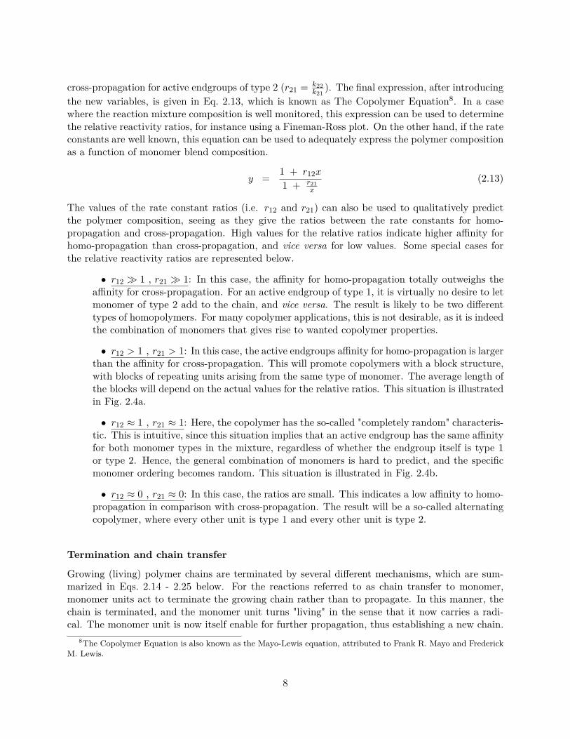
). The final expression, after introducingthe new variables, is given in Eq. 2.13, which is known as The Copolymer Equation8. In a casewhere the reaction mixture composition is well monitored, this expression can be used to determinethe relative reactivity ratios, for instance using a Fineman-Ross plot. On the other hand, if the rateconstants are well known, this equation can be used to adequately express the polymer compositionas a function of monomer blend composition.

y = 1 + r12x

1 + r21x

(2.13)

The values of the rate constant ratios (i.e. r12 and r21) can also be used to qualitatively predictthe polymer composition, seeing as they give the ratios between the rate constants for homo-propagation and cross-propagation. High values for the relative ratios indicate higher affinity forhomo-propagation than cross-propagation, and vice versa for low values. Some special cases forthe relative reactivity ratios are represented below.

• r12 � 1 , r21 � 1: In this case, the affinity for homo-propagation totally outweighs theaffinity for cross-propagation. For an active endgroup of type 1, it is virtually no desire to letmonomer of type 2 add to the chain, and vice versa. The result is likely to be two differenttypes of homopolymers. For many copolymer applications, this is not desirable, as it is indeedthe combination of monomers that gives rise to wanted copolymer properties.

• r12 > 1 , r21 > 1: In this case, the active endgroups affinity for homo-propagation is largerthan the affinity for cross-propagation. This will promote copolymers with a block structure,with blocks of repeating units arising from the same type of monomer. The average length ofthe blocks will depend on the actual values for the relative ratios. This situation is illustratedin Fig. 2.4a.

• r12 ≈ 1 , r21 ≈ 1: Here, the copolymer has the so-called "completely random" characteris-tic. This is intuitive, since this situation implies that an active endgroup has the same affinityfor both monomer types in the mixture, regardless of whether the endgroup itself is type 1or type 2. Hence, the general combination of monomers is hard to predict, and the specificmonomer ordering becomes random. This situation is illustrated in Fig. 2.4b.

• r12 ≈ 0 , r21 ≈ 0: In this case, the ratios are small. This indicates a low affinity to homo-propagation in comparison with cross-propagation. The result will be a so-called alternatingcopolymer, where every other unit is type 1 and every other unit is type 2.

Termination and chain transfer

Growing (living) polymer chains are terminated by several different mechanisms, which are sum-marized in Eqs. 2.14 - 2.25 below. For the reactions referred to as chain transfer to monomer,monomer units act to terminate the growing chain rather than to propagate. In this manner, thechain is terminated, and the monomer unit turns "living" in the sense that it now carries a radi-cal. The monomer unit is now itself enable for further propagation, thus establishing a new chain.

8The Copolymer Equation is also known as the Mayo-Lewis equation, attributed to Frank R. Mayo and FrederickM. Lewis.

8

Figure 2.4: Illustration of typical block copolymers (a) and random copolymers (b).

Chain transfer to CTA proceeds in the same way, but instead of having a monomer unit termi-nate the growing chain, the chain transfer agent of the system is responsible. For termination bychain recombination, two growing chains meet and terminate each other by combining to a longer(dead) chain. The mechanistic idea of this phenomenon is drawn in Fig. 2.5. Chain termination bydisproportiation is somewhat similar to termination by recombination, in that two living polymerchains meet and terminate each other. For chain disproportiation, however, the resulting productsare two dead chains instead of one long chain. These two chains have different characterics at theendgroup, with one being unsaturated (having a double bond in the chain). The mechanism forthis effect is drawn in Fig. 2.6. [2]

Chain transfer to monomer:

Mi(s)− P1 + M1kf11−−−→Mi(s)−D1︸ ︷︷ ︸

"Dead" chain

+ P1︸︷︷︸"Living" monomer

(2.14)

Mi(s)− P1 + M2kf12−−−→Mi(s)−D1 + P2 (2.15)

Mi(s)− P2 + M1kf21−−−→Mi(s)−D2 + P1 (2.16)

Mi(s)− P2 + M2kf22−−−→Mi(s)−D2 + P2 (2.17)

Chain transfer to CTA:

Mi(s)− P1 + CTAkf,CT A1−−−−−→Mi(s)−D1 + P1 (2.18)

Mi(s)− P2 + CTAkf,CT A2−−−−−→Mi(s)−D2 + P1 (2.19)

Termination by chain recombination:

Mi(s)− P1 + Mi(r)− P1ktc,11−−−→Mi(s)−M1 −M1 −Mi(r) (2.20)

Mi(s)− P2 + Mi(r)− P1ktc,21−−−→Mi(s)−M2 −M1 −Mi(r) (2.21)

Mi(s)− P2 + Mi(r)− P2ktc,22−−−→Mi(s)−M2 −M2 −Mi(r) (2.22)

Termination by chain disproportionation:

Mi(s)− P1 + Mi(r)− P1ktd,11−−−→Mi(s)−D1 + Mi(r)−D1 (2.23)

Mi(s)− P1 + Mi(r)− P2ktd,21−−−→Mi(s)−D1 + Mi(r)−D2 (2.24)

Mi(s)− P2 + Mi(r)− P2ktd,22−−−→Mi(s)−D2 + Mi(r)−D2 (2.25)

9

For modeling purposes, the large amount of kinetic rate constants are usually reduced by combining

Figure 2.5: Mechanistic idea for polymer termination by chain recombination.

Figure 2.6: Mechanistic idea for polymer termination by chain disproportiation.

some of them to yield common rate constants. Cross-species chain transfer to monomer is modeledas the geometric average of the homo-species transfer, as indicated in Eq. 2.26. The homo-specieschain transfer to monomer, which is indicated in Eq. 2.27, is modeled in the same spirit as theArrhenius-approaches for the previously modeled reaction rate constants.

kfij =√kfiikfjj , i, j = 1, 2 (2.26)

kfii =kfii,0 exp

(−Efii

RT

)kfii,adj

(2.27)

The reaction rate constants for chain transfer to CTA can be modeled in an easy way, by simplycombining the contributions from the two types of endgroups, as indicated in Eq. 2.28. Here, anadjustment factor is included aswell.

kf,CTA = kf,CTA1 + kf,CTA2kf,CTA,adj

(2.28)

For the termination reactions, the rate constants are combined into two rate constants, as indicatedin Eqs. 2.29 & 2.30. These are again combined and adjusted as shown in Eq. 2.31.

ktc = ktc,11 + ktc,21 + ktc,22 (2.29)ktd = ktd,11 + ktd,21 + ktd,22 (2.30)

kT = ktc + ktdkT,adj

(2.31)

This concludes the listing of the possible chemical reactions in the copolymerization system.

10

Phase distribution

A classic illustration of the nature of emulsion copolymerization is presented in Fig. 2.7, in orderto give an overall representation of the behavior of these types of systems. This serves to sumup the preceding subsections on emulsion copolymerization, and motivate the discussion of phasedistribution in such systems.

Figure 2.7: A classic illustration of emulsion polymerization.

There are three different phases typically considered in emulsion copolymerization processes,which are all included in Fig. 2.7. The aqueous (water) phase, represented by the white space inthe figure, is largely made up of the water fed to the reactor, which acts as a bulk phase, dissolvingthe two other phases. Because of this, water is an important component within the system withrespect to solubility issues, heat transfer properties both between the various phases and withexternal components, etc. The water phase is also the phase in which most of the initiator, CTAand emulgator/surfactant9 is dissolved. The aqueous phase can hold both monomer and polymer,but the solubility of these species are usually very low, sometimes even negligible, compared to thesolubility in the droplet (monomer) phase and the particle (micelle) phase. The micelles in whichthe polymer chains form and elongate are usually referred to as the particle phase of the emulsionsystem. The micelles hold both initiator and CTA, in relatively small concentrations, while themain part of the micelles are polymer chains or unreacted monomer units. The third phase in the

9Surfactant: Surface active agent. Surfactants are chemical species which align at the interphase boundaries inmultiphase systems such as emulsions, dispersions, etc. and act to either promote or prevent phase separation. Sincesurfactants most often are added in very small quantities, and don’t participate in chemical reactions, the surfactantsare often omitted from the modeling for simplicity.

11

emulsion system is the monomer droplet phase, which is made up of unreacted monomer particleswhich have yet to travel to the particle (micelle) phase to participate in polymer chain propagation.The behavior of the droplet phase depends on the nature of the monomer particles, but also on theoperation of the reactor. In several applications, reactors are run under so-called monomer starvedconditions, in which the monomer droplet phase will be negligible. To achieve monomer starvedconditions, the monomers are typically added carefully along the batch time in a typical semi-batchmanner, such that a large excess of monomer is avoided at the beginning of the batch.

In certain copolymerization processes, the gas phase of the system must also be considered.Whether this is necessary or not depends on the nature of the monomers in the system in connectionwith the operating conditions of the reactor. In several cases for emulsion copolymerization, both inindustrial and lab-scale experiments, the modeling of the gas phase is not crucial for the successfulmodeling of the liquid part of the reactor system.

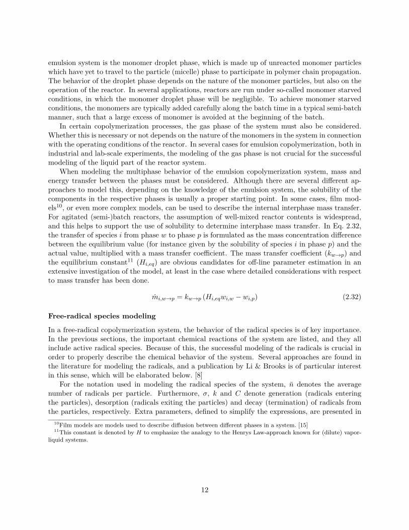
When modeling the multiphase behavior of the emulsion copolymerization system, mass andenergy transfer between the phases must be considered. Although there are several different ap-proaches to model this, depending on the knowledge of the emulsion system, the solubility of thecomponents in the respective phases is usually a proper starting point. In some cases, film mod-els10, or even more complex models, can be used to describe the internal interphase mass transfer.For agitated (semi-)batch reactors, the assumption of well-mixed reactor contents is widespread,and this helps to support the use of solubility to determine interphase mass transfer. In Eq. 2.32,the transfer of species i from phase w to phase p is formulated as the mass concentration differencebetween the equilibrium value (for instance given by the solubility of species i in phase p) and theactual value, multiplied with a mass transfer coefficient. The mass transfer coefficient (kw→p) andthe equilibrium constant11 (Hi,eq) are obvious candidates for off-line parameter estimation in anextensive investigation of the model, at least in the case where detailed considerations with respectto mass transfer has been done.

mi,w→p = kw→p (Hi,eqwi,w − wi,p) (2.32)

Free-radical species modeling

In a free-radical copolymerization system, the behavior of the radical species is of key importance.In the previous sections, the important chemical reactions of the system are listed, and they allinclude active radical species. Because of this, the successful modeling of the radicals is crucial inorder to properly describe the chemical behavior of the system. Several approaches are found inthe literature for modeling the radicals, and a publication by Li & Brooks is of particular interestin this sense, which will be elaborated below. [8]

For the notation used in modeling the radical species of the system, n denotes the averagenumber of radicals per particle. Furthermore, σ, k and C denote generation (radicals enteringthe particles), desorption (radicals exiting the particles) and decay (termination) of radicals fromthe particles, respectively. Extra parameters, defined to simplify the expressions, are presented in

10Film models are models used to describe diffusion between different phases in a system. [15]11This constant is denoted by H to emphasize the analogy to the Henrys Law-approach known for (dilute) vapor-

liquid systems.

12

Eqs. 2.33 & 2.34.

φ = 2(2σ + k)2σ + k + C

(2.33)

q =√k2 + 4σφC (2.34)

The three approaches for radical species modeling which has been considered in the modeling workfor the copolymerization case (see Sec. 3.3) are listed below.

1. Using a dynamic full population balance for particles carrying between 0 and i radicals, withi being a number chosen in advance. Choosing a high value for i gives more complexity,which in turn demands more computational power, but it also increases the accuracy of theradical model. Using a full population balance, the radical model becomes as indicated inEqs. 2.36 - 2.38. For this purpose, it is necessary to formulate n as indicated in Eq. 2.35, i.e.a vector containing the amounts of polymer carrying the respective numbers of radicals.

n =

n0n1n2...ni

(2.35)

Here, n0 is the amount of polymer having zero radicals, n1 has one radical, etc. The changein the polymer species will then be given as indicated below.

dn

dt= An (2.36)

A =

−σ k 2C 0 0 0 0 . . .σ −σ − k 2k 6C 0 0 0 . . .0 σ −σ − 2k − 2C 3k 12C 0 0 . . .0 0 σ −σ − 3k − 6C 4k 20C 0 . . .0 0 0 σ −σ − 4k − 12C 5k 30C . . ....

. . . . . . . . . . . . . . . . . . . . .

(2.37)

dn

dt= 1NT

[0 1 2 · · · i

] dndt

(2.38)

Here, NT denotes the total number of particles in the system, which is assumed to be con-stant12 for these equations to hold. The complete strategy for constructing the A-matrixis given in App. A, where a MATLAB-script is provided to illustrate the general approach,depending on the chosen value for i.

12A constant number of particle in an emulsion copolymerization system is usually valid when seed particles forpolymerization is used.

13

2. Using a steady state approximation for average number of radicals per particle. Li & Brookshave written a comprehensible text where the topic is approximations to the full populationbalance [8]. One of the outcomes is the steady-state approximate solution for the averagenumber of radicals per particle, as indicated in Eq. 2.39. Using this approximation, thenumber of dynamic states for the system is reduced, but the model loses some of its accuracy.

n = 2σ 1− exp(−qt)(k + q)− (k − q) exp(−qt) (2.39)

3. Using a dynamic Li-approximation for average number of radicals per particle. The strategyin this case is similar to the steady state approximation, but an important difference is thatthe average number of radicals per particle is maintained as a dynamic state of the system.The formulation of this approximation is as indicated in Eq. 2.40. [8]

dn

dt= σ − kn− φCn2 (2.40)

Among these different approaches, the latter is the most used in this work, because it gives a satisfy-ing trade-off between accuracy and complexity. This leads to satisfying computational time withoutcompromising the detail of the model too much. A comparison between the three, illustrated foran entirely fictitious case13, is illustrated in Fig. 2.8. This example shows that the dynamic Li-approximation agrees very well with the full population balance. The steady state-approximationalso shows decent agreement, apart from the behavior at the very start of the simulation.

Copolymer product quality parameters

There are several quantities to calculate in order to investigate the quality/state of the copolymerproduct. The most common identifier for a copolymer blend is the molecular weight distributionof the copolymer. Usually, two different formulations for molecular weight is used, as presentedin Eqs. 2.41 & 2.42, which in turn can be used to formulate a quantity known as PolydispersityIndex (PDI), as presented in Eq. 2.43. A comprehensible text on molecular weight distribution forpolymer systems is written by Crowley and Choi, made specifically for a free-radical polymerizationsystem for control purposes [13]. The use of polymer moments for characterizing the copolymersystem is also discussed by Gao and Penlidis [14] and Wyman [16], among others.

Number average molecular weight: Mn =m∑i=1

(YiMMi)µM1

1 + µM21 + µD1

µM10 + µM2

0 + µD0(2.41)

Weight average molecular weight: Mw =m∑i=1

(YiMMi)µM1

2 + µM22 + µD2

µM11 + µM2

1 + µD1(2.42)

Polydispersity index: PDI = Mw

Mn(2.43)

In these formulations, µji denotes the i’th order moment with respect to component j as active com-ponent. P1 and P2 denote active chains where the endgroup is monomer type 1 and 2, respectively,while D denotes dead/deactivated polymer chains. The various polymer moments are formulated in

13Here, dimensionless time is used along the time axis.

14

Figure 2.8: A plot showing the agreement between the three various approaches for radical speciesmodeling, for a fictitious case. Curves show average number of radicals per particle versus dimen-sionless time.

a systematic manner in the appendix, App. B. Furthermore, Yi denotes the abundance of monomertype i in the polymer, i.e. the relative consumption of monomer type i, while MMi is the molecularweight for each monomer unit of type i.

The degree of monomer conversion is another important quantity to calculate. This is discussedbriefly in the section for semi-batch reactor modeling, Sec. 2.2, and two alternative formulationsfor monomer conversion is presented in Eqs. 2.53 & 2.54. In most copolymerization processes, theconversion of monomer is desired to be as high as possible. For reasons related to the kinetics ofthe system, this is not always achievable within the time limits of the batch.

2.2 Fundamentals of semi-batch reactor modeling

The semi-batch reactor is a popular reactor design for applications in polymer synthesis industry.One of the main reasons for this is the ability to better control the feeding of reactants, andhence indirectly control the temperature changes in the reactor in a desirable way. This is a hugeadvantage, because temperature control is of key importance in many polymer applications, bothwith respect to product quality and safety. This section provides a short introduction to modelingof semi-batch reactors from a general point of view. [6][7]

The semi-batch reactor has several similarites to the regular batch reactor which, by assump-

15

tion, is a perfectly mixed tank reactor with no gradients, neither with respect to concentration,temperature or any other intensive quantity, in spatial coordinates. Under this assumption, themodeling is simplified, but the reactor design accounts for time variation. It is important to notethat a regular batch reactor does not allow for convective fluid transport across the reactor bound-ary during the course of the reaction. For a batch reactor, in its most simple form, the designequations (which are the component mass balances and energy balance, respectively) can hence bewritten as indicated in Eqs. 2.44 & 2.45.

Mass balances: dNi

dt= riV i = 1, .. , n (2.44)

Energy balance: dU

dt= Q+Ws (2.45)

In this formulation, Ni is the amount of species i, U is the internal energy of the reactor, V (t)is the (time dependent) volume of the reactor contents, ri is the reaction rate of component i, Ws

is the shaft work applied to the system, which is usually negligible, while Q is the energy changeassociated with external heat transfer (heating, cooling, heat loss, etc.). This model describes asystem with n chemical species, each with its independent mass balance. The reaction rate of eachcomponent in the system (ri) can be modeled in several ways, depending on the complexity andthe nature of the chemical reactions. A common approach is to calculate the reaction rate usinga rate law, in which the reaction rate is assumed to vary with the concentration of the respectivecomponent to some order, like indicated in Eq. 2.46. In this expression, k indicates the order ofthe rate law, and ki is a reaction rate constant, for example calculated as indicated in Eq. 2.9 forthe copolymerization case. In Eq. 2.9, the Arrhenius temperature dependency of the reaction rateconstant is used, and this is a widespread approach for modeling kinetics of this kind.

ri = kicki (2.46)

In some applications, assumptions can be made to simplify the model equations further. Forinstance, a so-called temperature explicit energy equation can be achieved under the assumptionthat the heat capacity (indicated by Cp in Eq. 2.47) of the reactor content is time independent. Thisassumption often holds for aqueous solutions, among other systems. In cases where this assumptiondoes not hold, the heat capacity should be modeled dynamically as a temperature function in orderto achive the temperature explicit form of the energy balance. The motivation for obtaining atemperature explicit energy balance is that the instensive property temperature appears muchmore tangible than energy. The fact that the measuring of temperature can be performed in astraight-forward manner for many applications also makes temperature a preferred quantity overenergy. Another simplification for the model equations comes along when the total volume of thereactor content can be assumed to be constant as time passes in the reactor. Using ci = Ni

V (whereci denotes the concentration of species i), this simplifies the molar mass balances. These commonsimplifying cases are given in Eqs. 2.47 & 2.48.

Mass balances: dcidt

= ri , i = 1, .. , n (2.47)

Energy balance: mCpdT

dt= Ws +Q (2.48)

The model equations for the batch reactor are the basis for the approach towards a semi-batchreactor model which, in addition to "just" being a time dependent reaction vessel, also allow for

16

external mass transfer across the reactor boundary. In the COOPOL copolymerization reactorprocess, which is the basis for this work, for instance, the reactants are added gradually during thereaction time, instead of adding them all at the start of the reaction (which would be the regularbatch reactor approach). Another strategy of interest could be to extract product gradually duringthe course of the batch, which is also allowed in the semi-batch reactor approach. The reactordesign now approaches the nature of a continuous reactor, in which CSTR14 probably is the closestrelative. Effects from the flowing fluids, both with respect to species mass balances and the energybalance must now be added, and the volume of the fluid contents must be given attention as well.

Mass balances: dNi

dt= riV (t) + ni =⇒ d

dt(ciV (t)) = riV (t) + ni

=⇒ V (t)dcidt

+ cidV

dt= riV (t) + ni (2.49)

In Eq. 2.49, ni is the net flowrate of species i to the reactor, i.e. the difference between theinflow and the outflow. In this general approach, effort is made to emphasize that the species massbalances hold for formulations on both molar basis and mass basis, as long as the correspondingreaction rates etc. are treated in agreement with this, i.e. using the correct units. The mass basisis perhaps the most established and intuitive approach, and this is mainly due to the principle ofconservation of mass. This enables the development of useful equations to describe the system,e.g. volume balances15 or dynamic equations for the composition of the respective species in thereactor. In the expression below (Eq. 2.51), ρ is the density of the fluid mixture residing in thereactor.

dmtot

dt= min − mout (2.50)

=⇒ d

dt(ρV ) = min − mout

=⇒ ρdV

dt+ V

dρ

dt= min − mout (2.51)

This equation can be combined with the species mass balances, Eq. 2.49, to eliminate the derivativeof the volume from the mass balance if desired, but that also raises the need for a differentialequation in time expressing the density variation. In many cases, simplifications can be introducedto make the model easier to treat, yet still represent reality in a good way. For instance, for afluid with constant density and no fluid flow out of the reactor, this equation intuitively reduces toEq. 2.52, which represents a special simplified case for the semi-batch reactor case. A conceptualdrawing of a semi-batch tank reactor is given in Fig. 2.9.

dV

dt= Vin (2.52)

The conversion of reactant in a semi-batch reactor can be formulated in several ways. InEqs. 2.53 & 2.54, two different formulations are shown for a batch simulated from t = t0 to t = t1

14Continuously stirred tank reactor: A time-invariant, perfectly mixed tank reactor.15The expression "volume balance" should be used with care, since the volume itself is not a conserved quantity.

In the same way an energy balance can manifest itself as an "enthalpy balance" in certain cases, the mass balancecan be reformulated to a "volume balance" if this is desired by the modeler.

17

Figure 2.9: Conceptual illustration of a semi-batch tank reactor with stirrer and continuous feeding.

in time. Here, R(t) denotes the molar amount of reactant in the reactor at time t and nR(τ) denotesthe net flow of reactant at time τ16. The two expressions have striking similarities, but while the"continuous" (also referred to as instantaneous conversion) formulation considers the conversionwith respect to accumulated monomer at time t, the "total" (also referred to as global conversion)formulation considers the conversion with respect to accumulated monomer at time t1. That is,the total amount of monomer for the entire batch time. For the considerations done with respectto parameter fitting in Sec. 4.1, the "total" formulation is applied.

"Total" formulation: X(t) =R(t0) +

∫ tt0nR(τ)dτ −R(t)

R(t0) +∫ t1t0nR(τ)dτ

(2.53)

"Continuous" formulation: X(t) =R(t0) +

∫ tt0nR(τ)dτ −R(t)

R(t0) +∫ tt0nR(τ)dτ

(2.54)

With this in mind, attention can be given to the energy balance of the reactor. The semi-batchreactor is an open system, and the energy balance will take effect from the mass flow dynamicsof the semi-batch reactor. This represents a difference from the regular batch-reactor, which is aclosed system without external convective flows. In the following expression, h and h0 denote thespecific enthalpy of the fluid in the reactor and the fluid feed, respectively. Note that due to theassumption of a perfectly mixed reactor vessel, the intensive properties will be the same in theentire reactor, and the specific enthalpy of the exiting fluid will hence be that of the uniform fluidresiding in the reactor. The simplified energy balance, where external shaft work applied to thereactor is neglected17, is proposed in Eq. 2.55. In addition, the enthalpy changes due to chemical

16The greek letter τ is here introduced to be used as an integration variable, with the main purpose being to avoidconfusion when it comes to the variable t denoting time.

17This assumption does not generally hold. For many tank reactors, however, it does hold despite the fact that

18

reactions in the reactor system is important to consider in the modeling work.

dU

dt= Q+ min · h0 − mout · h (2.55)

For many reactor applications, the very purpose of modeling the energy balance is to achieveinformation about the temperature, which is a quantity of key importance in most cases, withrespect to monitoring the behavior of the system. For a typical free-radical copolymerizationreaction system for instance, as described in Sec. 2.1, the reactor temperature is of key importancefor both the performance and safety considerations of the chemical reactor. Another reason forbothering with having the temperature as a key process variable is the fact that temperature,in contradiction to energy and enthalpy, is an intuitive and tangible quantity. For many reactorapplications, the temperature is also easy to measure without having to deal with a significant timedelay, thus providing a safe and reasonably accurate indirect measure of the state of the reactor.By modifying the energy balance (Eq. 2.55), the expression in Eq. 2.56 is achieved, thus allowingto specifically monitor the change in temperature over time for the reactor.

d

dt

mRcp,R(T − Tref )︸ ︷︷ ︸Reactor vessel

+ mcp(T − Tref )︸ ︷︷ ︸Reactor contents

= Q+ min · h0 − mout · h

=⇒ dT

dt= Q+ min · h0 − mout · h

mRcp,R +mcp(2.56)

In typical semi-batch reactor cases, the collection of balance equations add to yield a systemof ordinary differential equations which must be solved simultaneously. This concludes the briefdiscussion on first principles modeling of semi-batch reactors. These concepts were applied whenthe model for the specific copolymerization case, which is described in Sec. 3.3, was developed.

2.3 Introduction to off-line estimation and constrained optimization

When designing models from first principles, most of the parameters used in the modeling work aremore or less uncertain, as they are approximated, guessed from experience with similar systems,etc. Some parameters may even be entirely fictional due to "shortcuts" taken by the modeler. Anexample of such a case could be the interphase mass transfer for a system in which the diffusionis very complicated to describe. The specific phase(s) may even be assumed to be ideally mixed,leading to a case without intraphase concentration gradients and mass transfer. In such a case,a good strategy could be to soften the interphase18 mass transfer process with a fictional timeconstant, which in turn will be modified for the model to fit reality in a best possible way. Thescope of this section and the next is to motivate and explore the theory of both off-line and on-linestate and parameter estimation for implementations on dynamic systems. This is a crucial part ina (nonlinear) model-based controller implementation.

For a process model to be valid for a specific system, the measurable outputs as predicted bythe model need to match the reality as suggested by measurements from the corresponding real

the tank reactor is agitated, because the agitator contribution is small compared to the contributions from chemicalreactions and cooling/heating.

18Emphasis is made to notify the distinction between interphase (transfer between two separate phases) and in-traphase (transfer within one phase) mass transfer.

19

system. The constant (or weakly varying) parameters of the system must, in other words, bechosen such that the system outputs agree with measurements. With this motivation, methods foroff-line parameter estimation are deployed to adjust, and thus improve, a model by modifying aset of parameters, such that the output predicted by the model agrees with reality (experimentaldata measurements) to a satisfying degree. As indicated in the previous paragraph, the total set ofparameters may include parameters which are known to a sufficient degree, while some parametersare quite uncertain. From these, the most uncertain should be subject to modification while thecertain parameters should generally remain the same. In this sense, the parameter estimation is apreliminary method of improving the process model prior to the on-line implementation. A generalequation system for the model of a dynamic system is presented in Eqs. 2.57 - 2.59. Here, x is thevector of states for the system, u is the vector of inputs, while θ denotes the vector of parameters.That is, all the parameters for the system, which are assumed to be constant or weakly varyingthrough the course of time (t) for the system. The respective values of the parameters may be moreor less uncertain for this general case.

dx

dt= f(x, u, θ, t) (2.57)

0 = g(x, u, θ, t) (2.58)yp = h(x, u, θ, t) (2.59)

For this kind of system, given a vector of measurements in time (ym), a selection of parameters(η) is chosen from the entire collection of parameters (θ), which will be subject to modification.For super-simplified models with few parameters, the modification can be achieved by manuallyadjusting the parameters in a trial-and-error manner in which the agreement between the model andthe measurements is evaluated by the modeler. The systematic approach to parameter modification,however, is achieved by solving an optimization problem in which the sum of the deviations betweenthe model predictions and the measurements is minimized. For most cases encountered in real-lifeapplications, the process models are nonlinear and complex, containing a variety of parameters.The parameters are often interconnected with the states in an intricate manner, such that theimmediate effect on the overall system behavior from changing the respective parameters maynot necessarily be entirely intuitive. These characteristics all point toward using the systematicapproach rather than the (tedious) trial-and-error approach. The general optimization problem tobe solved is represented, mathematically, in Eq. 2.60. [12]

minη

N∑k=1

(yp,k(x, u, θ, t)− ym,k)2 (2.60)

η ∈ θ

s.t. dx

dt= f(x, u, θ)

0 = g(x, u, θ)

The Cybernetica ModelFit software, for which a brief introduction is provided in Sec. 3.2, isable to establish and solve these kinds optimization problems for off-line cases in an elegant manner,but an advantage of using this software is the potential of extending the parameter estimation toon-line use. In addition, the software can include intial values for the states of the system into the

20

optimization problem. An alternative way to do off-line parameter estimation is to use the built-in MATLAB function lsqcurvefit, which is a least squares curve fitting tool, approximatingparameter values for a function to fit data. The formulation is as presented in Eq. 2.61 which,generally speaking, is completely analogous to the problem introduced in Eq. 2.60. In this case,F (x, θ) is a general nonlinear function which is evaluated at discrete points in time (k), eachcorresponding to a measured value for the function output (yk). Both x and θ are inputs to thefunction, but θ denotes the vector of parameters which is desired to be recalculated for the functionto fit measurements better. By minimizing the sum of squares of the deviation between the modelprediction and the measured value with respect to θ, optimal θ-values are found for the function.

minθ

N∑k=1

(Fk(x, θ)− yk)2 (2.61)

This approach is analogous to the strategy for off-line parameter estimation performed in theCybernetica ModelFit software, which is evident from the comparison of Eq. 2.61 with Eq. 2.60.The Cybernetica ModelFit software is briefly described in Sec. 3.2.

Solving optimization problems of this type can be complicated, mainly because the functioninvolved is nonlinear. In addition, the problems are often constrained. Unconstrained globallyconvex19 problems with quadratic cost functions are relatively managable to solve, but this classof problems are not often encountered when treating real-life processes. Usually, the optimizationproblems are only locally convex or maybe not convex at all due to the nonlinearity and complexityof the system models. In dealing with real-life applications, the parameters are physical parametersin the sense that they cannot contradict common sense or the laws of nature. The optimizationproblems hence have to be provided with sensible constraints to maintain the physical validityof the solution. Examples of invalid situations are negative valued volumes and negative valuedspecies concentrations. Another example could be heat transfer coefficients, in which the optimiza-tion problem may suggest values which greatly exceed previously recorded values for the specificmaterials involved. Common for these cases is that while the solution may be feasible and sensiblein a mathematical sense, the physical interpretation is invalid. Because of this, the importance ofsensible parameter constraints when performing parameter estimation is emphasized.

For a linear function, the solution to the optimization problem would be relatively straight-forward to formulate and find, because this leaves a quadratic optimization problem. Methodsfor quadratic programming (QP) are well-established, and such problems are usually solved usingline-search methods (LSM). Typical LSMs are the Steepest Descent Method, the Newton Methodand various Quasi-Newton methods (in which the Hessian matrix from the Newton Method isapproximated to decrease the computational effort). While details on these methods are omittedfrom this text, the strategy is to first decide the best direction of step in space20. Based on this,the step length is calculated, and this alternating procedure is carried out at each iteration ofthe solution method. Alternatively, so-called trust region methods (TRM) could be deployed, inwhich a region for the solution of the problem is expanded or contracted depending on whether theobjective function is adequate in the region or not. [11]

When the system equations are nonlinear, the optimization problems turn more difficult to solve.19Convexity is an important property in numerical optimization. For a convex problem, a local minimum will also

be the global minimum and hence the optimal solution to the problem. [11]20Space here referes to the entire space of the system, i.e. the dimensions of the system. For x ∈ Rn, this would

mean n-dimensional space. A step in space simply denotes changes in the respective variables in n-space.

21

Several approaches and algorithms exist to treat problems like this. Among them are differentiation-free optimization (DFO) methods like the Nelder-Mead21 algorithm, but the most common approachis probably the strategy of sequential quadratic programming (SQP). In this case, the optimizationproblem is reformulated as an approximate quadratic problem, which is solved as a series of QPs inan iterative manner. The Cybernetica ModelFit software (Sec. 3.2) uses SQP to solve optimizationproblems in which the model functions are nonlinear. The MATLAB alternative for optimizingnonlinear functions is the built-in fmincon function, in which a nonlinear optimization problemis solved with given constraints using an SQP algorithm. A thorough walkthrough on the solutionstrategy for SQP problems is not provided in this text. For more details on numerical optimization,the reader is referred to more extensive texts, e.g. Nocedal & Wright. [11]

A continuation to the theory of estimation for dynamic systems is provided in the next section,in which state and parameter estimation is considered for on-line applications.

2.4 On-line estimation and filtering

For on-line implementations, estimation of both states and parameters remain as important sub-jects. A block diagram illustration22 of a typical MPC implementation is provided in Fig. 2.10. The

Figure 2.10: A conceptual block diagram showing the idea of an MPC controller scheme.

figure illustrates the roles and interconnection of the key components of such an implementation.Here, CVs denote controlled variables (i.e. system outputs), MVs denote manipulated variables(i.e. system inputs) and DVs denote disturbance variables to the system. In this setup, the esti-mator block is included, in close connection with the process model block. It is emphasized thatthe degree in which the process model represents the actual process depends on the quality of theprocess model. In most applications, there are deviations between the two, and to account forthis is the quintessential purpose of the estimator. In other words, the estimator will continuouslyreinforce the process model depending on the outputs from the real process. The efficiency of theestimator is, conversely, largely dependent on the quality of the process model, as this provides the

21This algorithm is attributed to John Nelder & Roger Mead. The algorithm is also known as the Downhill SimplexMethod or the Amoeba Method.

22This figure is printed with the permission of S. O. Hauger, Cybernetica AS.

22

basis for the estimator algorithm. The success of these mutual interactions will in turn enable thecontroller to choose the best possible action with respect to the controller objectives. The scope ofthis section is to perform a brief investigation of the behavior of the estimator block in Fig. 2.10.Extensive texts on on-line estimation are available, and the findings in this work is largely basedon Nocedal & Wright [11], Rawlings & Mayne [17] aswell as Simon [18]. In addition, the study hasbeen inspired by a comprehensible publication on dynamic estimation, including Kalman filtering,written by Schei [12].

When considering on-line estimation, there are several approaches to choose from when devel-oping an estimator algorithm. The most common class of approaches is probably the estimatorclass known as the Kalman filter (KF). A systematic development of the Kalman23 filter estimatorequations for dynamic systems is provided in the appendix to this text, App. C. This additionalsection is included to establish a more complete theoretical background for the purpose of on-lineestimation of states and parameters. A justification for locating this section in the appendix is thefact that these considerations remain largely theoretical, and without immediate implications forthe results of this specific project work. The established theory for on-line estimation will, however,be crucial in the proposed extension to this work, where model-based predictive controller design,i.e. the controller block of Fig. 2.10, is considered. In such an event, all the components needed foran MPC implementation would be considered. Because of this, some of the results from App. Care presented and discussed here.

For the purposes of treating free-radical copolymerization reactors, systems with a high degreeof nonlinearity are encountered, and the theory of estimation need to account for these effects. Asdiscussed in App. C.3, there are several approaches to treat nonlinear systems. With increasingcomplexity comes increasing accuracy, and consequently also a larger demand for computationaleffort. One of the most straight-forward methods to deploy is the so-called Extended Kalman filter(EKF), which is elaborated in App. C.3. App. C is devoted to derive the various formulations forthe Kalman filter depending on the characteristics of the system, and the most essential results arereproduced here.

For a system having both continuous dynamics and continuous measurements, the equationsfor the EKF become as indicated in Eqs. 2.62 - 2.64. In this case, both process noise (w) andmeasurement noise (v) are continuous variables with covariances Q and R, respectively.

˙x = f (x, u, w∗, t) +K (y − h (x, v∗, t)) (2.62)K = PCT R−1 (2.63)P = AP + PAT + Q− PCT R−1CP (2.64)

In this consideration, x is the state estimate, and ˙x denotes the state estimate derivative with respectto time. Kk is the gain of the Kalman filter, which uses the deviation between measured output(y) and predicted output (h (x, v∗, t)) to update the state estimates. P is the covariance vector forthe state estimates, while A is a system matrix originating from the formulation of the continuoussystem (Eq. C.1). These results are derived for a system in which both the model dynamics andthe measurements are continuous, but this may not necessarily always be the case. In most real-lifeapplications encountered, the dynamic system is modeled using a continuous formulation, whilemeasurements are only available at specific points in time. To overcome this challenge, the so-called Hybrid EKF can be deployed, in which the formulations for continuous and discrete KF are

23Attributed to Rudolf E. Kàlmàn (1930 - ), award-winning Hungarian-American mathematical systems theoryscientist and electrical engineer.

23

combined to account for the behavior of the real-life system. In such an event, the equations forthe estimator become as shown in Eqs. 2.65 - 2.69.

Between t+k and t−k+1: ˙x = f (x, u, w∗, t) (2.65)P = AP + PAT + Q (2.66)

Between t−k and t+k : Kk = P−k HTk

(HkP

−k H

Tk + Rk

)−1(2.67)

x+k = x−k +Kk

(yk − hk

(x−k , v∗, tk

))(2.68)

P+k = (I −KkHk)P−k (I −KkHk)T +KkRkK

Tk (2.69)

Here, xk is the state estimate at time tk, where x−k and x+k denote the a priori and a posteriori state

estimates, respectively. Kk is the Kalman filter gain, which uses the deviation between measuredoutput (yk) and predicted output (hk

(x−k , v∗, tk

)) at time tk to decide the correction between the

a priori and a posteriori state estimate. Like for the EKF in Eqs. 2.62 - 2.64, P is the covariancefor the state estimates, with P−k and P+

k denoting the a priori and a posteriori covariances at timetk, respectively. A still represents the system matrix from the formulation of the continuous system(Eq. C.1).

Up until now, this entire section aswell as App. C have been largely aimed at state estimation.This is undoubtedly an important subject, but the development of the estimator algorithms foron-line state estimation also allows for on-line parameter estimation. In Sec. 2.3, the parametersof the system were referred to as constant or weakly varying. In the latter case, an interestingtask is to use the estimator algorithm to also estimate parameters, and not only the states of thesystem, according to the measurements. In contrast to the strategy of Sec. 2.3, where preliminaryoff-line parameter estimation was introduced, this represents a method to address changes in weaklyvarying parameters for on-line use. From the total set of parameters for the system (θ), a sub-set(η) was chosen for optimization in the off-line parameter estimation study preliminary to the on-linecase. Among these, some parameters (λ) may be expected to vary during the course of time forthe system. These parameters are added to the vector of states as indicated in Eq. 2.70, and theresulting state vector (x′) is referred to as the augmented state vector. It is emphasized that thenew model function (f ′) is a reformulated edition of the original function (f), which accounts forthe changes made in x to yield x′. The new model function also includes process noise affectingthe parameters (wλ), which is the source of changes in the parameter values.

x′ =[xλ

](2.70)

x′ = f ′(x′, u, w,wλ

)(2.71)

Apart from the reformulation where the state vector has been extended to yield the so-calledaugmented state vector and the model function is adjusted, the estimator algorithms will be thesame as before. The established estimator equations can hence be used directly, keeping in mindthat the estimates now contain both state estimates and parameter estimates. The measurementfunction (h/hk) must also be adjusted in agreement with this.

24

3 Model description and software featuresThis section introduces the software tools utilized in the work. Sec. 3.1 aims to introduce theprogramming language Modelica, which has been used to formulate the models used in the work.A brief description of the Dymola software, which is deployed to treat the Modelica code, is alsoprovided. In Sec. 3.2, the Cybernetica ModelFit software is introduced, which is used for parameterfitting and simulations of the process model. A walkthrough of an example for a simplified stringpendulum is provided in the appendix, App. F, in which the purpose is to illustrate the use of thevarious software tools that were deployed for the main case of the project work. While this representsa simple model (with only two states and two parameters), the example still illustrates the elegancywith which the process model can be formulated in Modelica and exported to the CyberneticaModelFit software for simulation and parameter fitting. This example does not, however, illustratethe potential of assigning various subunits in a modular/hierarchical manner, but this is elaboratedfor the main reactor modeling case in Sec. 3.3.

Sec. 3.3 is written to include details and characteristics for the specific copolymerization caseconsidered in this work, which is a semi-batch free-radical emulsion copolymerization process.Details on the specific reactor system are protected under confidentiality of the COOPOL project,and details on the respective monomers of the system has been omitted. The monomers are simplyreferred to as monomer 1 and monomer 2. Details on the batch time are also omitted, and scaleddimensionless time has been used for the simulation. With the established theoretical backgroundfrom Secs. 2.1 & 2.2, the specific reactor system is described. The treatment of this reactor systemis considered in Sec. 4.

3.1 A brief introduction to Modelica & Dymola

Modelica is a programming language for object-oriented programming which was first released in1997. Since then, the language has been developed to treat a range of applications within differentfields, and although Modelica may not be the most abundant programming language with respectto world-wide use, the applications are numerous, for instance in the automotive industry. In beingobject-oriented, Modelica has similarities to classic programming languages like C++ or Java,but it also has differences, and Modelica is often referred to as a modeling language rather thana programming language. Among the strengths are easy declaration and treatment of variables,aswell as strong performance with respect to numerical efficiency and computational time. Anexample of a Modelica script is presented in Fig. F.2 in App. F, in which the dynamic model for asimplified pendulum is implemented as an example.

The Modelica language is excellent for solving DAE-systems1. The mathematical representationof such a problem is formulated in Eqs. 3.1 & 3.2. Eq. 3.3 shows how measurements from theprocess are predicted from the state of the system, but this measurement prediction is a concern ofthe application to a real system rather than a concern for the Modelica modeling in itself.

x = f(x, u, θ, t) (3.1)0 = g(x, u, θ, t) (3.2)yp = h(x, u, θ, t) (3.3)

1DAEs: A system of differential and algebraic equations, in contrast to ODE-system, which only contains ordinarydifferential equations.

25

In this formulation, x is the vector of states for the system, yp is the vector of predicted systemoutputs corresponding to a vector of measurements from the real system (ym), u is the vectorof inputs to the system, and θ is the vector of parameters. The functions f , g and h indicategeneral functions for the system, describing the nature of the system. The dot-notation is used toindicate differentiation with respect to time. This is, generally speaking, the same system that wasintroduced for the general discussion of parameter fitting and numerical optimization in Sec. 2.3.

Dymola2 is a proprietary software for implementation of Modelica code. In that sense, Dymolasupports both editing, compilation and simulation (i.e. numerical integration etc.) of Modelicacode. When solving problems like the one in Eqs. 3.1 & 3.2, Dymola deploys powerful algorithmswhich account for stiffness problems, etc. In addition to this, Dymola is able to produce simulationplots and data files for use in other applications. A valuable feature of the Modelica/Dymolacombination, which is mentioned in Sec. 3.2, is the possibility of exporting the whole model, andnot only the simulation results, to other applications using the so-called model exchange.

A special treat of Dymola is the opportunity to use a graphical user interface (GUI), whichenables the user to perform graphical drag-and-drop modeling of processes, given the desired com-ponents/subunits of the process3. In Fig. 3.5 in Sec. 3.3, the graphical interface is displayed for areactor test case. This promotes the use and development of modeling libraries for various types ofprocesses, and represents a large potential with respect to reusability and modificability of models,which can prove to be a huge advantage to the modeler. With these possibilities, Dymola canbe used as a dynamic process simulator, like Aspen Plus or Aspen HYSYS, with the option ofmanipulating each unit4 as desired using the Modelica language. This fascilitates a large degree ofcustomization in the modeling work. Using a modular and hierarchical approach to modeling alsoenables the modeler to interchange and/or modify certain parts of the model without compromisingthe respective other components or the overall structure of the model. This strategy is illustratedin Fig. 3.1. Fig. 3.1a and Fig. 3.1b show two different approaches for modeling a specific system,whereas Fig. 3.1b is the modular approach. The two approaches yield the same overall model, andthe simulation results will be similar, but the advantage of the modular approach is, as alreadymentioned, the possibility of easily exchanging certain parts/components without compromisingthe total structure of the model. The benefits of this strategy are elaborated in Sec. 3.3, when thespecific test case for the copolymer reactor is introduced and described.

3.2 The Cybernetica ModelFit software

Cybernetica ModelFit is a software developed by Cybernetica AS for state and parameter esti-mation. The ModelFit software is designed to work alongside software for nonlinear model-basedpredictive control (NMPC), but ModelFit is in itself a model simulator tool which can be used torun ballistic model simulations and perform off-line parameter fitting, which is the purpose of thiswork.

To utilize the ModelFit software, the traditional approach is to formulate the specific processmodel in the programming language C, as this provides a suitable basis for importing the model

2Dymola: Dynamic Modeling Laboratory, software developed by Dassault Systemes AB, Sweden.3The approach of designing subunits which are combined to yield the complete process model, rather than creating

one single large model script, is referred to as the modular approach.4One of the main drawbacks of Modelica/Dymola in comparison with the mentioned commercial process simulator

tools is the fact that apart from the fields of electrical circuit modeling, mechanical modeling and fluid flow modeling,the standard libraries of Dymola are scarce. Because of this, the modeler is sometimes required to make components"from scratch" or adopt components made by a third-party contributor.

26

Figure 3.1: A figure showing the general idea of interconnecting Modelica units in a hierarchy.

into the ModelFit software. ModelFit is, in other words, programmed to recognize the variousfeatures of the model from the formulation of the model script. For models formulated in otherenvironments than C, a technique5 for so-called model exchange exists, which is referred to as theFunctional Mock-up Interface (FMI). The FMI is a tool to establish a platform which enables thecommunication between models and applications initially formulated in different languages. Oneof the supported languages in the FMI is Modelica, and this motivates the use of Modelica forthese kinds of applications, in agreement with the introduction given in Sec. 3.1. Modelica modelscan, in other words, easily be exported to the ModelFit software, and the ModelFit software willeven recognize which variables are inputs and which variables are outputs, given that the Modelicamodel is formulated correctly. The FMI translation tool, which is relatively easy to administer, isimplemented in the Dymola software.

Given an imported model, e.g. using the model exchange strategy as introduced above, Mod-elFit can be used to test models, and perform off-line parameter fitting using given experimentalmeasurements. ModelFit has built-in routines for treating DAEs, where the user can choose amongseveral alternatives. Simple Euler-integration is available, where the user is inclined to set steplength of the method, and a mid-point Euler method is also implemented. The most sophisticatedtool available to the user for solving the system equations is the CVODEs tool6. The choice ofsolution method depends on the complexity and stiffness of the system. The trade-off betweencomputational time and accuracy/convergence of the solution may also play a part in deciding thesolution method.

In the procedure for calculating the optimal parameter values for a model to fit experimentalmeasurements, the software solves a minimalization problem with respect to a chosen set of pa-rameters, in which the sum of squares for the deviations between the model predictions and theexperimental measurements is desired to be as low as possible. This is formulated mathematicallyin Eq. 3.4.

5The FMI is developed as a part of the MODELISAR European project, which had the german automotivecompany Daimler AG among its main initiators and contributors.

6CVODEs is a tool developed under the SUNDIALS (Suite of Nonlinear and Differential/Algebraic equationSolvers) project at the Center for Applied Scientific Computing of the Lawrence Livermore National Laboratory,designed for numerical solution of stiff DAEs. [9]

27

minη

nky∑k=1

(yp,k − ym,k)2 (3.4)

η ∈ θ

In this formulation, yp,k and ym,k are model predictions and measurements, respectively, for thesample point k. The number of valid measurements is represented by nky, while η is the selectionof parameters among all the parameters (θ) which are chosen for optimization.

For setting up and solving these kinds of optimization problems, the ModelFit software hasseveral additional features. The software is constructed to provide a user-friendly way to decidewhat parameters to estimate, i.e. to decide η from θ. If the user also wishes to estimate initialvalues for the states of the system, these variables are accessed and activated for estimation inthe same simple manner as for the parameters. In agreement with what was mentioned regardingthe physical interpretation of the parameters in Sec. 2.3, the maximum and minimum values forthe respective variables are easily accessible for the user. In addition to this, ModelFit providesvaluable supporting calculations during the course of the optimization procedure, making it easierfor the user to evaluate the quality of the solution. One of these calculated quantities is the scaledHessian condition number, for which an example is illustrated in Fig. 3.2. Generally speaking, thecondition number indicates how the output value of a function will respond to a change in the inputvalue(s). For the case of parameter fitting, the function in mind is the cost function as introduced inEq. 3.4. A high value for the condition number for the scaled Hessian matrix is usually an indicationthat some of the parameters in the set has low individual sensitivities towards the cost function.Another possible cause of a high value for the condition number is linear dependence between someof the optimization variables. A way of resolving this could be to re-evaluate the combination ofoptimization variables (η). Another quantity calculated for the respective optimization variables isthe identifiability ranking, for which an example is shown in Fig. 3.3. The identifiability rankingcan be interpreted in somewhat of the same way as the condition number for the Hessian matrix, inthat it indicates the sensitivity of the respective optimization variables on the cost function. In thisconsideration, however, the variables are ranked, and the user is able to better decide which variablesto dismiss when re-choosing variables for optimization. A low identifiability ranking usually impliesa low sensitivity to the cost function for that specific variable or a strong linear dependence to oneof the other variables. In other words, the variables with the lowest identifiability rankings are themost sensible candidates for being dismissed from the optimization procedure. Both Figs. 3.2 & 3.3originate from the parameter fitting procedure described in Sec. 4.3, but for the purpose of thissection, they are included to portray the features of the ModelFit software. [21]

In App. F, the ModelFit software is demonstrated for a simplified model of a pendulum. In thiscase, the two parameters of the model are modified to yield virtually perfect agreement betweenthe output predicted by the model and the reality as suggested by corresponding measurements.Because of the simplicity of the model, Eulers method for solving the equation system was cho-sen, using a short step-length, and the solution and simulation of the system proceeded withoutproblems. The strategy for treating the main case of this project work (Sec. 3.3) is completelyanalogous to the example in App. F, apart from the fact that the CVODEs solver is chosen forthe main case because of stiffness related issues for the system. In addition to this, the main casealso presents with a significantly higher amount of both states and parameters than the simplifiedexample. Because of this, it is expected that deciding variables for optimization, i.e. choosing η

28

Figure 3.2: Changes in the condition number for the scaled Hessian matrix in the model fittingcalculation.

Figure 3.3: Changes in the identifiability ranking for the variables during model fitting calculation.

29

from θ, may be harder than for the pendulum example, for which the choice of optimization vari-ables was obvious. Nevertheless, the general solution strategy remains the same, and the benefitsof using the ModelFit tool are evident in both cases.

This concludes the short introduction to the Cybernetica ModelFit software, which will beutilized when performing parameter fitting for the emulsion copolymerization process described inSec. 3.3. The results from the off-line parameter fitting are presented in Sec. 4.

3.3 Model description for the established model on emulsion copolymerization

The purpose of this section is to establish the remaining details regarding the reactor systemtreated in Sec. 4, referred to as the main case of the project work. The theoretical background forthe established model is presented in Secs. 2.1 & 2.2, and this provides the basis for the modelingwork. All balance equations, i.e. energy balances and species mass balances are constructed asindicated in Secs. 2.1 & 2.2, with reaction kinetics etc. as suggested. The model is formulated inthe Modelica language using the Dymola tool, as introduced in Sec. 3.1.

The studied process is a semi-batch free-radical emulsion copolymerization process in whichtwo different monomer types are combined to yield a copolymer product. The process is initiatedusing polymer seed particles and a chemical initiator compound. The tank reactor is assumed to beperfectly mixed due to agitation of the content. In this spirit, the system has been modeled withoutspatial gradients. This implies good internal mixing in each of the phases present in the reactor,aswell as rapid transfer of both heat and mass between the respective phases. From a modelingpoint of view, this will avoid the need for partial differential equations (PDEs) to describe thesystem, since ordinary differential equations (ODEs) with respect to time will suffice to describethe dynamic system. In the modeling work, the monomer droplet phase of the system is assumedto be negligible, and the gas phase of the system has not been considered in the modeling workas this is not believed to contribute significantly to the overall behavior of the reactor system. Inthis sense, the system is an entirely liquid system (emulsion), in which a polymer particle phase("oil phase") and an aqueous phase ("water phase") are considered. The neglecting of the monomerdroplet phase is in agreement with the semi-batch reactor strategy where reactants (monomer)are added slowly over the course of time for the batch, thus achieving so-called monomer starvedconditions. The feeding to the reactor is illustrated in Fig. 3.4, where the feeding is split into threeseparate streams which are individually controllable. Feed stream 1 contains water and emulgator,feed stream 2 contains monomer (approximately 80/20 wt% M1/M2) and some CTA, while feedstream 3 contains initiator dissolved in water. The continuous feeding of reactants is abortedhalfway through the course of the batch, for the remaining reactants to react completely.

The cooling mechanism for the reactor is a jacket covering most of the reactor wall. Direct heatloss from the reactor to the surrounding environment occurs at the spots which are not covered bythe jacket, and these areas are located at the top and bottom of the reactor. The cooling jacket,which for this installation usually contains water with temperatures in the range 70-90 oC, willexperience heat loss to the surroundings depending on the exposed surface area.

The main characteristics of the established model with respect to inputs and outputs are givenin Tab. 3.1. The responsibility of a controller for such a reactor is to control both the feeding ofreactants aswell as the amount of cooling fluid fed to the system in accordance with the controllerobjectives. Notice that the temperature of the cooling fluid may be either a disturbance to thesystem or an input, which is dependent on the specific plant for which the reactor model is applied.In some cases, the cooling fluid is given by an uncontrollable part of the process like an upstream

30

Figure 3.4: Illustration of the feeding to the reactor during the time of the batch.

unit or a cooling water reservoir. In other cases, the cooling fluid is the product of a supportingprocess built specifically for providing cooling fluid. In the latter case, where the temperature ofthe cooling fluid will be controllable, the controller will also add this quantity to the list of inputs inorder to achieve the controller objectives. Notice also that the reactor temperature is representedby two separate temperatures, i.e. the temperatures of the respective phases in the system. Thisseparation is a consequence of a choice made in the modeling work, i.e. to model the energy contentsof the two phases separately. Because of good mixing in the reactor, the two temperatures will forall intents and purposes be equal, and will both pose a valid measure of the reactor temperature inoverall. It is emphasized that although the main disturbances to the process are listed (Tab. 3.1),changes in the DVs are not considered in the simulations.

Table 3.1: Model characteristics for the established semi-batch case.

Important MVs Important CVs Important DVsMass flow, Feed stream 1 Temperature, reactor Temperature, surroundingsMass flow, Feed stream 2 Composition, particle phase Temperature, cooling fluidMass flow, Feed stream 3 Composition, aqueous phase Temperature, feed streamsMass flow, cooling fluid Degree of monomer conversion Composition, feed streamsTemperature, cooling fluid Polymer molecular weight

Polydispersity Index

Throughout the text, the fact that the the model is constructed from first principles is empha-sized, along with the fact that certain parameters are initially fictional. While this is largely true,some empirical correlations are deployed in the modeling, and most of the physical data for thesystem are acquired from the litterature. A brief collection of fluid properties for the system ispresented in App. D. An important empirical part of the model is the properties for heat transferbetween the contents of the reactor vessel, the cooling fluid in the cooling jacket and the surround-

31

ing environment. These models are developed for a small lab-scale tank reactor, where the thermalconductivities are modeled as a linear function of the total volume of the contents of the vessel, i.e.the sum of the volumes for the respective phases in the reactor. These correlations are shown inEqs. 3.5 & 3.6, in which kASR and kASJ denote the thermal conductivity between the surroundingenvironment and the reactor vessel and the cooling jacket, respectively. Here, the volume of thevessel content (V ) is given in litre (dm3). It is emphasized that these correlations may not holdfor reactors with a different geometric shape and different size, and this may raise the need forparameter fitting if the model is deployed for similar reactors with different cooling mechanisms.The experimental data used in the work (App. E) was acquired using a lab-scale reactor, hencejustifying the choice of heat transfer properties for this case.

kASR = 0.018264V + 0.55210 (3.5)kASJ = 0.8591641V + 1.502800 (3.6)

During the modeling work, effort was made to make the models receptive to parameter fit-ting/estimation. In this spirit, most internal processes such as chemical reactions, interphase masstransfer, etc. are formulated using parameters with adjustment/correction factors. Having estab-lished this, parameter estimation for an internal process can be performed by approaching thecorresponding adjustment factor for the process rather than directly approaching the parametersthemselves. In doing this, the original parameter values, which may be acquired from the lit-terature, are kept intact. The parameters themselves may in turn be changed, but this shouldpreferably be done after careful evaluation of the results from the parameter fitting procedure.

Figure 3.5: Graphical Dymola representation for a reactor test case.

The established case for the reactor system as it appears in the GUI of Dymola is shown in

32

Fig. 3.5. At this layer of the model, the reactant feeding and cooling to the system are showntogether with the top layer of the semi-batch reactor model. The entire code for the model isnot included in this report, mainly because the code is extensive despite the fact that the modelis declared as a combination of various subunits. This strategy is inspired by the idea proposedin Fig. 3.1b in Sec. 3.1, and for the specific reactor case, the hierarchical structure becomes asillustrated in Fig. 3.6. The Reactor block in Fig 3.5 is, in other words, not in itself a complexunit with an extensive code attached to it, but rather a top layer governing the interconnectionand communication between the various subunits of the model. These subunits can range from thecooling jacket model, the model for the reactor vessel itself, or the thermodynamics of the fluidsinvolved, as indicated in Fig. 3.6.

Figure 3.6: A figure showing the interconnection of Modelica units for the semi-batch copolymer-ization reactor system in a hierarchical manner.

An important aspect of the model is the reusability and the opportunity to modify the modelin an easy way. The modular approach in designing subunits of the model (Fig. 3.6) is of keyimportance with respect to this. An additional feature of Modelica, which strengthens this strategy,is known as fluid package modeling. Instead of modeling each chemical species of the reactor systemas an individual fluid, the respective phases of the system are assigned to a fluid package each. Inthis sense, the physical state, the thermodynamic state, the phase composition, etc. of the phasesin the reactor are stored and accounted for by a fluid package, while the changes in the fluid aregoverned by the balance equations provided in the reactor model subunit, etc. The benefit of thisstrategy is the ability to change the components of the system, e.g. using different monomer species,by introducing a new fluid package. This would require only minor changes to the other subunitsof the overall system. In this work, only one case has been considered, but to achieve adaptablemodels for long-term use, these features are valuable, and has hence been included in the modelingwork.

This concludes the description of the semi-batch reactor system considered in this work. Thetreatment of this system with respect to parameter estimation is considered in Sec. 4.

33

4 Results from off-line parameter estimationThis section presents the results from the main task of the project work, which is to validatethe established process model for semi-batch emulsion copolymerzation. This section starts off byinvestigating the behavior of the original model (as introduced in Sec. 3.3) in Sec. 4.1. Here, thepurpose is to explore to what extent the model predictions deviate from the provided measurements,and identify the main reasons for the deviations. The experimental basis is a lab-scale test reactor,for which the experimental data is summarized in App. E. In Sec 4.2, these findings are used toexplore how the model changes with respect to manual changes in certain parameter values. Basedon the indications from the trial-and-error approach in Sec. 4.2, the Cybernetica ModelFit software(Sec. 3.2) has been used to perform optimal parameter fitting, as described in Sec. 4.3. Finally,a short summary evaluating the characteristics and performance of the model after the optimalparameter fitting is presented in Sec. 4.4.Note: The simulations in this section are all given with masked time axes. The reason for thisis that details regarding the batch time is confidential information under the COOPOL project.This modification to the simulations is not believed to pose a deterioration of the results and theconclusions of the work.

4.1 Model behavior before parameter fitting

As a starting point for discussing the validity of the developed models, the models are compared (intheir original first principles form) to experimental data. In Fig. 4.1 the conversion of reactant isplotted for both the process model (red curve) and experimental lab-scale experiments1 (blue curve).The conversion is here defined as indicated in Eq. 2.53 in Sec. 2.2. In Fig. 4.2, the temperature ofthe particle phase2 in the reactor is shown for both model predictions (red curve) and measurements(blue curve). In addition, the development of the molecular weight of the copolymer product isshown in Fig. 4.3. For the molecular weight distribution, the experiments only give the terminalvalues, i.e. the values at the very end of the batch. From these preliminary results, it is evident thatthe established process model deviates somewhat from the truth as portayed by the experiments.The characteristics of the two curves for the conversion are similar, yet the actual values deviateto some extent. A summary of the most important differences between the model predictions andthe measurements, as indicated by this initial consideration, are listed below.

1. The model prediction has a lower conversion than the experiments have. This effect is evidentfor most of the batch simulation time, especially at the end.

2. The experiments approach steady state (100% conversion) faster than the model predictiondoes. In fact, the model prediction does not reach 100% conversion at all during the simulationtime.

3. The molecular weights show agreement with experimental data with respect to their relativeratio, i.e. the polydispersity index, but the respective values are significantly lower than theexperiments suggest.

1The experimental data is found in the appendix, App. E2In agreement with what was discussed about fluid package modeling in Sec. 3.3, the respective phases of the

system will have individual temperatures. Since the reactor is assumed to be well agitated, the heat transfer betweenthe phases is rapid, and hence the temperature of the phases will be virtually equal. The particle phase temperatureis, in other words, a representative measure of the overall reactor temperature.

34

Figure 4.1: A plot showing the conversion of fed monomer to the reactor, before parameter fittinghas been performed.

Figure 4.2: A plot showing the temperature of the particle phase in the reactor, before parameterfitting has been performed.

35

Figure 4.3: A plot showing the molecular weights (weight and number average) of the copolymerproduct, before parameter fitting has been performed.

The differences are, generally speaking, not tremendous, yet they are significant, and hence theyserve as an indication that parameter estimation is needed for the model. As illustrated in thetemperature plot (Fig. 4.2), the temperature agreement between the model prediction and theexperiments is very good. From these initial considerations, the actions suggested for furthertreatment of the model parameters are listed below.

1. Investigate and adjust the various factors governing the propagation, for the model to showbetter agreement with the consumption of monomer during the course of the batch time. Itis expected that the kinetic factors should be higher.

2. Investigate (and possibly adjust) factor(s) governing termination, in order to achieve closeto 100% conversion at the end of the batch time, and thus have better agreement withexperiments. Recalling how molecular weights are defined in Sec. 2.1 using polymer momentsfrom App. B, changing the parameters governing termination will also affect the molecularweights, which are important quantities for the product quality.

3. Adjust the heat conduction constant between the reactor vessel and the cooling jacket in orderto get even better agreement for the temperatures. Other factors governing the temperatureprofile of the reactor could also be investigated, but this is not first priority in validating themodel, since the model gives good agreement with the data when it comes to the temperatures.

These suggestions for change are considered in the following sections. It is emphasized that becauseof the complexity of the system, the various parameters may be interconnected in such a mannerthat the overall effect of changing each of them is non-trivial. The overall effect of changing acombination of parameters is usually even harder to predict using intuition.

36

4.2 Introductory case: Manual parameter fitting

The purpose of this section is to identify and explore how the model changes when some of the keyparameters are changed. For the purpose of this section, the changing of the parameters has beenperformed manually in a trial-and-error manner, simply to identify the qualitative behavior of themodel relative to the parameters. The optimal approach to parameter fitting is left for the sectionfollowing this one (Sec. 4.3).

In Fig. 4.4, the conversion of reactant is plotted for the model after the kinetic reaction rateconstants have been adjusted in a trial-and-error manner. As before, the blue curve represents themeasurements while the red curve shows model output. The motivation for this change is to gethigher conversion of monomer throughout the batch. The conversion does indeed increase whenthis change is applied, and close to 100% conversion is achieved at the end of the batch time. Theconversion is, however, slightly too high to agree with the experimental data during the first half ofthe simulation, and simply adjusting the kinetic factors does not appear to be a sufficient solution initself. In Fig. 4.5, the molecular weight distributions for the copolymer product is shown again, fortermination parameters fitted in a trial-and-error manner. The characteristic shape of the curvesas well as the ratio between the values, i.e. the polydispersity index as defined in Eq. 2.43, remainsapproximately the same, which is desirable3. In this sense, the model output for molecular weightdistribution has not changed much, but when it comes to the respective values for the molecularweights, the model predictions now agree with the experiments in a much more satisfying way.

Figure 4.4: Illustration of monomer conversion with kinetic reaction rate constants adjusted in atrial-and-error manner.

3A polydispersity index (Eq. 2.43) of just over 2 is expected for this reactor case, because a low degree of chainbranching is expected.

37

Figure 4.5: A plot showing development of copolymer molecular weight, after parameters governingtermination has been adjusted in a trial-and-error manner.

Generally speaking, there are still deviations between the model predictions and the measure-ments, and this fact motivates the strive for optimally fitted parameters. It is important to pointout that the optimal solution is not necessarily expected to yield perfect agreement between themodel predictions and the experimental measurements, but rather give the best possible resultgiven the chosen set of parameters for optimization. The actual changes made for the parametersin the trial-and-error approach are presented in Tab. 4.1. This serves as a starting point for theoptimal analysis of the parameters, which will be described in Sec. 4.3.

Table 4.1: Parameter changes for manual trial-and-error model fitting.Parameter Original value New valueAdjustment factor, 1-1 propagation rate constant 50 → 20Adjustment factor, 1-2 propagation rate constant 22 → 8Adjustment factor, 2-1 propagation rate constant 50 → 20Adjustment factor, 2-2 propagation rate constant 22 → 8Adjustment factor, monomer 1 transfer to CTA 20 → 55Adjustment factor, monomer 2 transfer to CTA 20 → 55

4.3 Optimal parameter fitting

In this section, the purpose is to further explore the adjustment factors for the system that wasinvestigated in Sec. 4.2. In addition, several other parameters are chosen for optimization. The

38

vector of parameters chosen for optimization (η) contains 11 parameters related to propagation,termination or interphase mass transfer. The respective parameters, with optimal changes, areshown in Tab. 4.2. For solving the optimization problems involved, the Cybernetica ModelFitsoftware (as introduced in Sec. 3.2) has been utilized, in agreement with the theoretical backgroundestablished in Sec. 2.3.

The resulting curve for the conversion of reactant after the optimization of the parameters isshown in Fig. 4.6. As before, the red curve indicates the model output. When being comparedto the result from the trial-and-error approach, as presented in Fig. 4.4, the differences are small.The results are similar in character, although the respective values of the parameters differ be-tween the two cases. The optimal case represents the solution with the lowest sum of deviations,mathematically speaking, and this is the solution of highest interest. It is emphasized that thetrial-and-error solution, although tedious, did not prove to be terrible compared to the optimalsolution. An interesting observation is that the trial-and-error approach (Fig. 4.4) actually yields

Figure 4.6: Figure showing monomer conversion, using optimally fitted parameters.

a higher conversion of monomer at the end of the batch than the optimal approach (Fig. 4.6) does.From this it can be interpreted that the initial difference (in the first half of the batch time) be-tween the conversion plots as suggested by the trial-and-error solution is larger than the differenceat the end of the batch time suggested by the optimal solution. It may, however, appear counter-intuitive and undesirable that the optimal solution has achieved lower conversion of monomer thanthe trial-and-error solution at the end of the batch. A way to work around this, if desired, wouldbe to weigh the deviations at the end of the batch time heavier, with respect to the cost function,than the deviations at the start of the batch time. In such an event, the deviations at the end ofthe batch would be penalized more than the deviations earlier in the batch, and the solution tothe optimization problem would change accordingly, "trying harder" to minimalize the deviations

39

at the end than the deviations in the start. This strategy has not been deployed in this work,however, and all measurement throughout the batch are considered equally important.

The curves for the molecular weight distributions of the system are shown in Fig. 4.7. By com-parison with the trial-and-error solution (Fig. 4.5), the two results are virtually the same, which isyet another good indication for the trial-and-error approach. The optimal solution does, however,represent the mathematically favorable and thus most interesting solution. It is emphasized thatalthough the two approaches yield a similar output with respect to the molecular weight distribu-tions, they have different combinations of parameter values. In Fig. 4.7, the experimental values

Figure 4.7: A plot showing copolymer molecular weights, using optimally fitted parameters.

for the molecular weights at the end of the batch are indicated as blue and green squares for thenumber and weight average molecular weight (Eqs. 2.41 & 2.42), respectively, to better displaythe agreement between the model output and the experimental measurements. The fact that themolecular weight distribution is only measured at the very end of the batch makes it difficult tosay anything about the characteristics of the development of the molecular weights throughout thebatch. In a case where the molecular weight distribution was measured several times throughoutthe batch, this would allow for a more thorough examination of the results, and perhaps even bettervalues for the fitted parameters.

The changes made to the respective parameters from the model chosen for optimization areshown in Tab. 4.2.

4.4 Summary: Model validity after optimal parameter fitting

This section is added to provide a brief summary of the achievements of the parameter fittingprocedure. The most important changes are listed below, and the specific changes made in theselected parameters are presented in Tab. 4.2.

40

Table 4.2: Parameter changes for optimal model fitting.Parameter Original value New valueAdjustment factor, 1-1 propagation rate constant 50 → 150.0Adjustment factor, 1-2 propagation rate constant 22 → 18.5673Adjustment factor, 2-1 propagation rate constant 50 → 68.3477Adjustment factor, 2-2 propagation rate constant 22 → 46.6841Common adj. factor for propagation 1 → 2.6914Common adj. factor for monomer transfer to CTA 1 → 2.975Adjustment factor, termination by recombination 800 → 1166.80Adjustment factor, termination by disproportiation 800 → 400.0Interphase mass transfer coefficient, monomer 1 100 000 → 102 264.93Interphase mass transfer coefficient, monomer 2 100 000 → 72 383.51Frac. between term. by rec. and total term. 1 → 0.8996

• The factors governing the rate of the propagation reactions have been modified for allfour possible propagation reactions. In addition, a common adjustment factor has beenintroduced for all four reactions. The results contribute to give better agreement between themodel output and the measurements for reactant conversion.

• The factors governing termination have been adjusted. Instead of adjusting the indi-vidual factors for monomer transfer to CTA, the two reactions have been combined in acommon adjustment factor. In addition, the respective adjustment factors for termination byrecombination and disproportiation has been optimized. The fraction between termination byrecombination has also been subject to optimization, that is the percentage of the total chaintermination accounted for by recombination, in agreement with the formulations in Sec. 2.1.This has led to better agreement between the model and the measurements with respect tothe molecular weight distributions.

• The softening coefficient ("fictional time constant") for species mass transfer between thephases of the system has been optimized for both monomer types. In this case, increasingthe coefficient will yield a slower mass transfer.

In total, the improved model presents with good agreement between the measurements and themodel outputs. The model presents with significant demands for computational power, and thismay pose a threat to the on-line use of the model in a complete controller implementation, but theparameter fitting itself is considered successful with respect to deploying a model-based predictivecontroller.

41

5 ConclusionsThe theoretical concepts for free-radical emulsion copolymerization have been established. Thishas been utilized to formulate a model in the programming language Modelica for a semi-batchcase on copolymerization of two different monomer types. The model was made largely from firstprinciples, and has been subject to off-line parameter estimation to fit the model to experimentaldata from a lab-scale reactor. The experimental reactor operates the same chemical system underthe same conditions, thus representing a corresponding real-life case to the established model.

For the purpose of off-line parameter estimation for the model, necessary theoretical backgroundwas explored, and software tools such as the Cybernetica ModelFit software was introduced. Themodel was initially treated by modifying certain parameters in a trial-and-error manner to investigethe agreement between model output and experimental measurements. The ModelFit software wasthen successfully utilized to perform off-line parameter fitting for the established model, adjusting11 of the parameters of the model to yield an optimal solution.

Trial-and-error adjustment of parameters is inaccurate and tedious in comparison to optimaladjusting, which is a systematic way to achieve decent parameter values. The results of the workshow, however, that the improvement from the trial-and-error solution to the optimal solution issmall when just a small selection of parameters is subject to modification. It is emphasized that theoptimal solutions are the desirable ones, although the trial-and-error solutions show good agreementwith the optimal solutions.

The computational time involved in solving optimization problems like the ones encountered inthe off-line parameter estimation of this work is definitely a concern to be taken into consideration.The computational effort is very important, in particular, when dealing with on-line systems andcontrol applications. The calculations in this work was performed off-line, yet they still serve toindicate the demand for computational effort for the model. The complexity of the process modelwas evident when performing SQP iterations to solve the parameter estimation problem, in whichscenarios with up to several minutes per iteration was experienced. The model used in this workmay, in other words, need improvements with respect to the numerical efficiency if the model isto be used for an on-line implementation. For the suggested extension to this work, which is thedesign of a nonlinear model-based predictive controller, this is exactly the case.

The theory of on-line estimation methods was explored, and this provides a basis for the devel-opment of estimator algorithms in the proposed extension to this work, where a complete controllerimplementation is considered.

42

References[1] PlasticsEurope, Plastics - the Facts 2012, An analysis of European Platics production, demand

and waste data for 2011, Belgium, 2012

[2] P. C. Painter & M. M. Coleman, Fundamentals of Polymer Science, 2nd Ed., CRC Press, 1997

[3] I. K. Khairullin, Adhesive-Melts - The Most Dynamically Developing Area in World Productionand Consumption of Adhesives, Pol. Sc. Series D, Glues and Sealing Materials, 2013, Vol. 6,No. 1

[4] H. Ghodke, S. Raman & B. E. Ydstie, Modeling and Control of Free Radical Co-Polymerization,Department of Chemical Engineering, Carnegie Mellon University, Pittsburgh, USA

[5] A. H. Helgesen, Toolbox for generation of nonlinear control models for semi-batch emulsionpolymerization reactors, Master thesis, Department of Chemical Engineering, Norwegian Uni-versity of Science and Technology, 2011

[6] A. Nyström, Modeling and Simulation of a Multi Phase Semi-batch Reactor, Master thesis,Department of Mathematical Sciences, Chalmers University of Technology & Göteborg Uni-versity, Gothenburg, Sweden, 2007

[7] H. S. Fogler & N. Gurmen, University of Michigan, Note on modeling of semi-batch reactors,2007, URL: http://www.umich.edu/~essen/html/06chap/html/prs_cstr.htm

[8] B. Li & B. W. Brooks, Prediction of the Average Number of Radicals per Particle for EmulsionPolymerization, J. Pol. Sc., Vol. 31, Iss. 9, Aug. 1993

[9] A. C. Hindmarsh & R. Serban, User Documentation for cvodes v2.7.0, March 2012, Centerfor Applied Scientific Computing, Lawrence Livermore National LaboratoryURL: http://computation.llnl.gov/casc/sundials/documentation/cvs_guide.pdf

[10] H. Olsson, H. Elmqvist & M. Otter, Modelica - A Unified Object-Oriented Language forSystems Modeling, Language Specification, Version 3.3, May 9, 2012URL: https://www.modelica.org/documents/ModelicaSpec33.pdf

[11] J. Nocedal & S. J. Wright, Numerical Optimization, 2nd Ed., Springer, 2006

[12] T. S. Schei, On-line estimation for process control and optimization applications, 8th Interna-tional IFAC Symposium on Dynamics and Control of Process Systems, Preprints Vol. 2, June6-8, 2007

[13] T. J. Crowley & K. Y. Choi, Calculation of Molecular Weight Distribution from MolecularWeight Moments in Free Radical Polymerization, Ind. Eng. Chem. Res. 1997, 36, 1419-1423

[14] J. Gao & A. Penlidis, Mathematical modeling and computer simulator/database for emulsionpolymerizations, Prog. Polym. Sci. 27 (2002) 403-535, Elsevier

[15] H. A. Jakobsen, Chemical Reactor Modeling: Multiphase Reactive Flows, Springer, 2008

43

[16] C. E. Wyman, Polymer Moment Equations for Distributed Parameter Systems, AlChE J., Vol.21, No. 2, 1975

[17] J.B. Rawlings & D. Q. Mayne, Model Predictive Control: Theory and Design, 2013, Nob HillPublishing, LLC

[18] D. Simon, Optimal State Estimation: Kalman, H∞ and Nonlinear approaches, 1st Ed., JohnWiley & Sons, 2006

[19] E. O. Kreyszig, Advanced Engineering Mathematics, 9th Ed., Wiley, 2005

[20] R. E. Walpole, R. H. Myers, S. L. Myers & K. Ye, Probability and Statistics for Engineers andScientists, 8th Ed., Pearson Education, 2007

[21] Cybernetica ModelFit User Manual, v. 1.20, Cybernetica AS

[22] Deliverable 4.6: Control model for industrial scale semi-batch polymerisation reactor, internalreport of the COOPOL project

44

A Additional information for radical species modelingWhen applying a full population balance to describe the radicals of the copolymerization system,as introduced in Sec. 2.1, the calculations use a system of equations involving a so-called A-matrix.The purpose of this matrix is to govern the respective changes in particles carrying between 0 andN radicals. The A-matrix is constructed as indicated in the MATLAB script1 in Fig. A.1.

In this script, sigma (σ), k and C represent the corresponding quantities from Sec. 2.1, while Ndenotes the maximum number of radicals per particle considered in the approach.

function [ dn ] = ndot_full( t, n )% ndot_full% function to calculate the time derivative of relative% radical frequency vector for emulsion polymerization

Li_parameters;N = max(size(n))-1; % Max. number of radicals per particle

A = [ -sigma k 2*C 0 zeros(1,N-3 );sigma -(sigma + k ) 2*k 6*C zeros(1,N-3 );zeros( N-1, N+1 ) ];

for i = 2:N,A(i+1,i) = sigma;A(i+1,i+1) = - sigma - i * k - i * (i-1) * C;if i < N,

A(i+1,i+2) = (i+1) * k;endif i < N-1,

A(i+1,i+3) = (i+2)*(i+1) * C;end

end

dn = A * n ;end

Figure A.1: MATLAB code for generating the A-matrix used in the full population balance, usedfor radical species modeling in Sec. 2.1.

1This script is printed with the permission of P. Singstad, Cybernetica AS.

I

B Polymer moments for copolymer product calculationsThis section presents the polymer moments used in the calculations for product quality. Thepolymer moments were introduced in Sec. 2.1 for calculating the molecular weight distribution forthe copolymer product, as described by Crowley and Choi [13]. The use of moments for describingthe molecular weight distribution is also described by Gao and Penlidis. [14]

The definition of the polymer moments is given in Eqs. B.1 - B.3. Here, i denotes the order ofthe moment, while [Pj(n)] denotes the concentration of living polymer med endgroup j, having alength of n units, etc.

µP1i =

∞∑n=1

ni [P1(n)] (B.1)

µP2i =

∞∑n=1

ni [P2(n)] (B.2)

µDi =∞∑n=1

ni [D(n)] (B.3)

Zeroth, first and second order moments, with respect to living chains with type 1 endgroup:

dµP10dt

= [M1][M1] + [M2]

2fIkInIVp

− kp12[M2]µP10 + kp21[M1]µP2

0

− kf12[M2]µP10 + kf21[M1]µP2

0 − φ (ktc + ktd)((µP1

0

)2+ µP1

0 µP20

)(B.4)

dµP11dt

= [M1][M1] + [M2]

2fIkInIVp

+ kp11[M1]µP10 + kp21[M1]

(µP2

0 + µP21

)− kp12[M2]µP1

1 − kf,CTA,1[CTA](µP1

1 − µP10

)− kf11[M1]

(µP1

1 − µP10

)+ kf21[M1]µP2

0 − kf12[M2]µP11 − φ (ktc + ktd)

(µP1

0 µP11 + µP1

1 µP20

)(B.5)

dµP12dt

= [M1][M1] + [M2]

2fIkInIVp

+ kp11[M1](µP1

0 + 2µP11

)+ kp21[M1]

(µP2

0 + 2µP21 + µP2

2

)− kp12[M2]µP1

2

− kf,CTA,1[CTA](µP1

2 − µP10

)− kf11[M1]

(µP1

2 − µP10

)+ kf21[M1]µP2

0

− kf12[M2]µP12 − φ (ktc + ktd)

(µP1

0 µP12 + µP1

2 µP20

)(B.6)

II

Zeroth, first and second order moments, with respect to living chains with type 2 endgroup:

dµP20dt

= [M2][M1] + [M2]

2fIkInIVp

+ kp12[M2]µP10 − kp21[M1]µP2

0

+ kf12[M2]µP10 − kf21[M1]µP2

0 − φ (ktc + ktd)((µP2

0

)2+ µP1

0 µP20

)(B.7)

dµP21dt

= [M2][M1] + [M2]

2fIkInIVp

+ kp22[M2]µP20 − kp21[M1]µP2

1 + kp12[M2](µP1

0 + µP11

)− kf,CTA,2[CTA]

(µP2

1 − µP20

)− kf22[M2]

(µP2

1 − µP20

)− kf21[M1]µP2

1 + kf12[M2]µP10 − φ (ktc + ktd)

(µP1

0 µP21 + µP2

1 µP20

)(B.8)

dµP22dt

= [M2][M1] + [M2]

2fIkInIVp

+ kp22[M2](µP2

0 + 2µP21

)− kp21[M1]µP2

2

+ kp12[M2](µP1

0 + 2µP11 + µP1

2

)− kf,CTA,2[CTA]

(µP2

2 − µP20

)− kf22[M2]

(µP2

2 − µP20

)− kf21[M1]µP2

2 + kf12[M2]µP10

− φ (ktc + ktd)(µP1

0 µP22 + µP2

2 µP20

)(B.9)

Zeroth, first and second order moments, with respect to dead chains:

dµD0dt

= kf,CTA,1[CTA]µP10 + kf,CTA,2[CTA]µP2

0 + kf11[M1]µP10

+ kf22[M2]µP20 + kf12[M2]µP1

0 + kf21[M1]µP20

+ φktc

(12µ

P10 µP1

0 + µP20 µP1

0 + 12µ

P20 µP2

0

)+ φktd

(µP1

0 µP10 + 2µP2

0 µP10 + µP2

0 µP20

)(B.10)

dµD1dt

= kf,CTA,1[CTA]µP11 + kf,CTA,2[CTA]µP2

1 + kf11[M1]µP11

+ kf22[M2]µP21 + kf12[M2]µP1

1 + kf21[M1]µP21

+ φ (ktc + ktd)(µP1

0 µP11 + µP2

0 µP11 + µP2

1 µP10 + µP2

0 µP21

)(B.11)

dµD2dt

= kf,CTA,1[CTA]µP12 + kf,CTA,2[CTA]µP2

2 + kf11[M1]µP12

+ kf22[M2]µP22 + kf12[M2]µP1

2 + kf21[M1]µP22

+ φktc(µP1

0 µP12 + µP1

1 µP11 + µP2

0 µP12 + 2µP2

1 µP11 + µP2

2 µP10 + µP2

0 µP22 + µP2

1 µP21

)+ φktd

(µP1

2 µP10 + µP2

0 µP12 + µP2

2 µP10 + µP2

2 µP20

)(B.12)

This system of differential equations provides a significant contribution to the total number ofstates for the model. This acts to increase the demand for computational power. The initializationof these states could also be subject to estimation, in addition to the estimation of the parametersof the system.

III

C Estimator derivationThis additional section is written to include details on the derivation of the Kalman filter (KF)equations used for on-line estimation, as discussed in Sec. 2.4. The definition of an estimator is ofkey importance when designing an on-line controller system, and may sometimes prove to be harderthan designing the controller itself. In Sec. C.1, the Kalman filter for a linear time-discrete systemis established as a starting point, and this is extended to continuous linear systems in Sec. C.2.In Sec. C.3, the (Extended) Kalman filter (EKF) for nonlinear systems is covered. The followingderivation adopts the approach, and hence the notation, of Simon. [18]

C.1 Kalman filter estimator for linear time-discrete systems

The starting point for the derivation of the Kalman filter is a linear time-discrete system. Thissystem is represented, in a general formulation, in Eqs. C.3 & C.4. In the case where the linearsystem is not time-discrete but continuous, which indeed is the case for most dynamic systems,the linear continuous system is converted to a discrete system. The formulation of the continuoussystem is shown in Eq. C.1, where the dotted notation indicates differentiation with respect totime.

x = Ax+Bu+ ω (C.1)

The discretized solution2 to such a system is indicated in Eq. C.2, in which xk is the vector of statesand uk is the vector of inputs at time tk. The discrete time interval tk − tk−1 is denoted ∆tk.

xk = eA∆tkxk−1 +∫ tk

tk−1eA(tk−τ) [B(τ)u(τ) + ω(τ)] dτ (C.2)

The general formulation for the linear time-discrete system is presented in Eqs. C.3 & C.4.

xk = Fk−1xk−1 +Gk−1uk−1 + wk−1 (C.3)yk = Hkxk + vk (C.4)

In this system, xk is the vector of states at the discrete point tk in time. The correspondingvector of measurements, yk, is represented by the sum of the state measurements (Hkxk) andthe measurement noise (vk). Here, Hk is a matrix deciding which of the states that go into themeasurement vector. Fk and Gk are the system matrices, governing how the states and inputs,respectively, at time tk affect the state at time tk+1. In special situations where F and G aretime independent (constant) matrices, the system is said to be linear time-independent (LTI). Theprocess noise at time tk is represented by wk. Both noise terms (wk and vk) are assumed to bezero-mean white noise with covariances3 Qk and Rk, respectively. The zero-mean assumption isjustified by the requirement that systematic mean-contributions from the noise are accounted forin the model, i.e. the system matrices. By comparison between the solution for the discretized

2These expressions contain mathematical terms such as matrix exponentials, convolution integrals, and othercomplex concepts. These concepts are not elaborated in this text, and the curious reader is referred to more extensivetexts for a walkthrough, e.g. Kreyszig. [19]

3Details on theoretical concepts from the field of statistics are omitted from this text. For theoretical backgroundon statistics, Walpole et. al. was consulted. [20]

IV

continuous system (Eq. C.2) and the general discrete system (Eq. C.3), the system matrices mustbe as indicated in Eqs. C.5 - C.7.

Fk−1 = eA∆tk (C.5)

Gk−1 =∫ tk

tk−1eA(tk−τ)Bdτ (C.6)

wk−1 =∫ tk

tk−1eA(tk−τ)ω(τ)dτ (C.7)

The purpose of the estimator is to propose an optimal estimate of the state at time tk (xk), andthis estimate is denoted xk. A distinction is made between a priori estimates and a posteriori4

estimates, which are denoted x−k and x+k , respectively. In this sense, whether an estimate at time tk

is a priori or a posteriori is a question of whether the measurement information at time tk is usedor not. Mathematically, this can be formulated as in Eqs. C.8 & C.9 for a priori and a posteriori,respectively. It is emphasized that x−k and x+

k are estimates of the same quantity, i.e. the statevector at time tk (xk).

x−k = E

[xk

∣∣∣∣ y1, y2, . . . , yk−1

](C.8)

x+k = E

[xk

∣∣∣∣ y1, y2, . . . , yk

](C.9)

Here, E [· · · ] denotes the expected value. As is evident from Eqs. C.8 & C.9, the two estimatesuse the same previous measurements (y1, y2, . . . , yk−1). The only difference is that the a posterioriestimate also utilizes the measurement at time tk (yk).

From this point on, Pk is introduced to denote the covariance of the state estimate error attime tk. Notice that the state covariance also has a distinction between a priori and a posterioriinformation, as indicated in Eqs. C.10 & C.11.

P−k = E

[(xk − x−k

) (xk − x−k

)T ](C.10)

P+k = E

[(xk − x+

k

) (xk − x+

k

)T ](C.11)

The system is initiated by an initial state, x+0 , having a covariance P+

0 . In the case where x+0 is

well known, the covariance (i.e. uncertainty) is zero, but in the case where x+0 is (very) uncertain,

P+0 approaches∞I. The next step is to analyze how the state estimates and covariances propagate

through time. Using the established definition in Eq. C.8 in combination with the proposed model inEq. C.3, the general propagation of state estimates becomes as indicated in Eq. C.12. A justificationfor this is that the process noise (wk) has a zero-mean propability distribution.

x−1 = F0x+0 +G0u0

General expression: x−k = Fk−1x+k−1 +Gk−1uk−1 (C.12)

4These terms are orginially known from philosophy. A priori and a posteriori mean "from the earlier" and "fromthe later", respectively, and these terms are used to describe the "quality" of the knowledge.

V

The propagation of the covariances is slightly more complicated. The approach starts from thedefinition in Eq. C.10, the model in Eq. C.3 and the result in Eq. C.12. The result, showing howthe covariances propagate in time, is provided in Eq. C.13.

P−k = E

[(xk − x−k

) (xk − x−k

)T ](xk − x−k

)= Fk−1xk−1 +Gk−1uk−1 + wk−1 − x−k

x−k = Fk−1x+k−1 +Gk−1uk−1

=⇒(xk − x−k

)= Fk−1

(xk−1 − x+

k−1

)+ wk−1(

xk − x−k) (xk − x−k

)T= Fk−1

(xk−1 − x+

k−1

) (xk−1 − x+

k−1

)TF Tk−1 + wk−1w

Tk−1

+ Fk−1(xk−1 − x+

k−1

)wTk−1 + wk−1

(xk−1 − x+

k−1

)TF Tk−1

=⇒ P−k = Fk−1P+k−1F

Tk−1 +Qk−1 (C.13)

This result was found by recognizing the expected value of each of the terms in the expression for(xk − x−k

) (xk − x−k

)T, once it was written out. This is illustrated in Eq. C.14. Eq. C.15 is in

agreement with the proposed covariance of the process noise, while Eqs. C.16 & C.17 agrees withthe fact that the estimation error

(xk − x−k

)is uncorrelated with the process noise (wk).

E

[Fk−1

(xk−1 − x+

k−1

) (xk−1 − x+

k−1

)T ]= Fk−1E

[(xk−1 − x+

k−1

) (xk−1 − x+

k−1

)T ]F Tk−1

= Fk−1P+k−1F

Tk−1 (C.14)

E[wk−1w

Tk−1

]= Qk−1 (C.15)

E

[wk−1

(xk−1 − x+

k−1

)TF Tk−1

]= 0 (C.16)

E[Fk−1

(xk−1 − x+

k−1

)wTk−1

]= 0 (C.17)

It has now been investigated how both state estimates and covariances propagate through timefor a linear time-discrete system, as indicated by Eqs. C.12 & C.13, respectively. These equationsgive the relationships for the transitions x+

k → x−k+1 and P+k → P−k+1, i.e. the propagation in time.

The next step is to formulate expressions for the transitions x−k → x+k and P−k → P+

k , i.e. thetransition from a priori estimates to a posteriori estimates at time tk. This is performed using theapproach of recursive least squares estimation. Having a measurement (yk) as indicated in Eq. C.4,the measurement correction is formulated as indicated in Eq. C.18. Here, Kk is the estimator gainmatrix, which becomes the Kalman filter gain when the errors between the states and the stateestimates are minimized.

x+k = x−k +Kk

(yk −Hkx

−k

)(C.18)

To minimize the estimation errors, a proper cost function5 is defined as indicated in Eq. C.19, in5In this formulation, Tr denotes the Trace of the matrix. This is a matrix operation which consists of calculating

the sum of the elements on the diagonal of the matrix.

VI

which the error ε is defined as shown in Eq. C.20.

Jk = E

[(x1 − x+

1

)2]

+ E

[(x2 − x+

2

)2]

+ · · ·+ E

[(xn − x+

n

)2]

= E[ε2x1,k + ε2x2,k + · · ·+ ε2xn,k

]= E

[εTx,kεx,k

]= Tr

(E[εx,kε

Tx,k

])(C.19)

εxi = xi − x+i (C.20)

The expected value for the vector of errors is needed, and this expression can be manipulated bycombining the error definition (Eq. C.20), the measurement definition (Eq. C.4) and the estimatormeasurement correction (Eq. C.18). The result is portrayed in Eq. C.21.

E [εx,k] = E[x− x+

k

]= E

[x− x−k −Kk

(yk −Hkx

−k

)]= E

[x− x−k −Kk

(Hkx+ vk −Hkx

−k

)]= E

[x− x−k −KkHk

(x− x−k

)−Kkvk

]= (I −KkHk)E

[x− x−k

]−KkE [vk] (C.21)

This result is possible to expand to give the expected value for the square of the error, as shown inEq. C.22.

E[εx,kε

Tx,k

]= (I −KkHk)E

[(x− x−k

) (x− x−k

)T ](I −KkHk)T

−KkE

[vk(x− x−k

)T ]+KkE

[vkv

Tk

]KTk

− (I −KkHk)E[(x− x−k

)vTk

]KTk

=⇒ E[εx,kε

Tx,k

]= (I −KkHk)P−k (I −KkHk)T +KkRkK

Tk (C.22)

This is achieved by recognizing the definition of P−k , aswell as remembering that the noises areuncorrelated with the error. Rk is, as postulated earlier, the covariance of the measurement noiseat time tk. These requirements are summarized in Eqs. C.23 - C.25.

P−k = E

[(xk − x−k

) (xk − x−k

)T ](C.23)

E[vk(x− x−k

)]= 0 (C.24)

E[vkv

Tk

]= Rk (C.25)

VII

Remembering the definition of P+k from Eq. C.11, these previous results also enable the formulation

of P+k , as represented in Eq. C.26.

P+k = E

[εx,kε

Tx,k

]=⇒ P+

k = (I −KkHk)P−k (I −KkHk)T +KkRkKTk (C.26)

The purpose in the next steps is to solve an optimization problem to uncover the optimalestimator gain, Kk, which is the Kalman filter gain. To do this, the cost function (accounting forthe estimator error), is differentiated with respect to Kk and set equal to zero. This procedure isshown in Eqs. C.27 - C.31. The step between Eq. C.30 and Eq. C.31 is performed by postulatingthat ∂(Tr(ABAT ))

∂A = 2AB, given that B is symmetric. In this case, this is assumed to be fulfilled.

∂J

∂Kk= 0 (C.27)

∂(Tr(E[εx,kε

Tx,k

]))∂Kk

= 0 (C.28)

∂

∂Kk

(Tr((I −KkHk)P−k (I −KkHk)T +KkRkK

Tk

))= 0 (C.29)

∂(Tr((I −KkHk)P−k (I −KkHk)T

))∂Kk

+∂(Tr(KkRkK

Tk

))∂Kk

= 0 (C.30)

2 (I −KkHk)P−k(−HT

k

)+ 2KkRk = 0 (C.31)

Eq. C.31 is reorganized to yield the final expression for the Kalman filter gain, which is shown inEq. C.32.

=⇒ Kk = P−k HTk

(HkP

−k H

Tk +Rk

)−1(C.32)

Finally, the resulting equations for the Kalman filter algorithm are listed in Eqs. C.33 - C.37.This system of equations is usually referred to as Riccati-equations.

P−k = Fk−1P+k−1F

Tk−1 +Qk−1 (C.33)

Kk = P−k HTk

(HkP

−k H

Tk +Rk

)−1(C.34)

x−k = Fk−1x+k−1 +Gk−1uk−1 (C.35)

x+k = x−k +Kk

(yk −Hkx

−k

)(C.36)

P+k = (I −KkHk)P−k (I −KkHk)T +KkRkK

Tk (C.37)

In some cases, it is desirable to combine the measurement updates and the estimation propagationin time to yield one expression including both. In other words, the a priori state estimate updatefrom time tk−1 to time tk is combined with the a posteriori update at time tk, and the same strategy

VIII

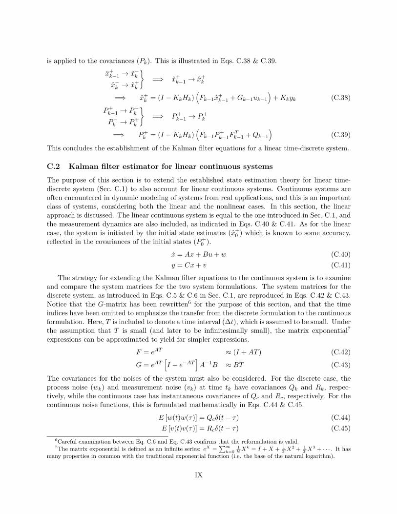
is applied to the covariances (Pk). This is illustrated in Eqs. C.38 & C.39.

x+k−1 → x−k

x−k → x+k

}=⇒ x+

k−1 → x+k

=⇒ x+k = (I −KkHk)

(Fk−1x

+k−1 +Gk−1uk−1

)+Kkyk (C.38)

P+k−1 → P−k

P−k → P+k

}=⇒ P+

k−1 → P+k

=⇒ P+k = (I −KkHk)

(Fk−1P

+k−1F

Tk−1 +Qk−1

)(C.39)

This concludes the establishment of the Kalman filter equations for a linear time-discrete system.

C.2 Kalman filter estimator for linear continuous systems

The purpose of this section is to extend the established state estimation theory for linear time-discrete system (Sec. C.1) to also account for linear continuous systems. Continuous systems areoften encountered in dynamic modeling of systems from real applications, and this is an importantclass of systems, considering both the linear and the nonlinear cases. In this section, the linearapproach is discussed. The linear continuous system is equal to the one introduced in Sec. C.1, andthe measurement dynamics are also included, as indicated in Eqs. C.40 & C.41. As for the linearcase, the system is initiated by the initial state estimates (x+

0 ) which is known to some accuracy,reflected in the covariances of the initial states (P+

0 ).

x = Ax+Bu+ w (C.40)y = Cx+ v (C.41)

The strategy for extending the Kalman filter equations to the continuous system is to examineand compare the system matrices for the two system formulations. The system matrices for thediscrete system, as introduced in Eqs. C.5 & C.6 in Sec. C.1, are reproduced in Eqs. C.42 & C.43.Notice that the G-matrix has been rewritten6 for the purpose of this section, and that the timeindices have been omitted to emphasize the transfer from the discrete formulation to the continuousformulation. Here, T is included to denote a time interval (∆t), which is assumed to be small. Underthe assumption that T is small (and later to be infinitesimally small), the matrix exponential7expressions can be approximated to yield far simpler expressions.

F = eAT ≈ (I +AT ) (C.42)

G = eAT[I − e−AT

]A−1B ≈ BT (C.43)

The covariances for the noises of the system must also be considered. For the discrete case, theprocess noise (wk) and measurement noise (vk) at time tk have covariances Qk and Rk, respec-tively, while the continuous case has instantaneous covariances of Qc and Rc, respectively. For thecontinuous noise functions, this is formulated mathematically in Eqs. C.44 & C.45.

E [w(t)w(τ)] = Qcδ(t− τ) (C.44)E [v(t)v(τ)] = Rcδ(t− τ) (C.45)

6Careful examination between Eq. C.6 and Eq. C.43 confirms that the reformulation is valid.7The matrix exponential is defined as an infinite series: eX =

∑∞k=0

1k!X

k = I + X + 12!X

2 + 13!X

3 + · · · . It hasmany properties in common with the traditional exponential function (i.e. the base of the natural logarithm).

IX

For this to hold for a small time interval T , it can be shown that the relationships between Q andQc and R and Rc must be as Eqs. C.46 & C.47, respectively. This is related to the total covarianceassociated with the entire time interval, i.e. sum of time intervals.

Q = Qc∆t (C.46)

R = Rc∆t (C.47)

Starting with the Kalman filter gain equation in Eq. C.34 from Sec. C.1, the corresponding termsfor the continous system are inserted to yield the continuous Kalman filter gain, as represented inEq. C.48.

Kk = P−k HTk

(HkP

−k H

Tk +Rk

)−1

Kk = P−k CT(CP−k C

T + RcT

)−1

Kk

T= P−k C

T(CP−k C

TT +Rc)−1

limT→0

Kk

T= P−k C

TR−1c (C.48)

The covariances for the states of the system also need attention. The covariance formulationsfrom Eqs. C.33 & C.37 are reproduced in Eqs. C.49 & C.50, respectively. For the purpose of thecontinuous formulation, the indices of the system matrices have been omitted, and Eq. C.33 hasbeen reorganized8.

P−k+1 = FP+k F

T +Q (C.49)P+k = (I −KkC)P−k (C.50)

For small values of T , the approximation in Eq. C.42 is valid, and the equation for the covariancesare developed as indicated below. The final result, known as the differential Riccati equation ispresented in Eq. C.51.

P−k+1 = FP+k F

T +Q

= (I +AT )P+k (I +AT )T +QcT

= P+k +

(AP+

k + P+k A

T +Qc)T +AP+

k ATT 2

= (I −KkC)P−k +A (I −KkC)P−k ATT 2

+[A (I −KkC)P−k p (I −KkC)P−k A

T +Qc]T

=⇒P−k+1 − P

−k

T= −KkCP

−k

T+AP+

k ATT

+(AP−k AKkCP

−k + P−k A

T −KkCP−k A

T +Qc)

=⇒ P = limT→0

P−k+1 − P−k

T= −PCTR−1

c CP +AP + PAT +Qc (C.51)

8The algebraic manipulation of the expression has been omitted from this text, but careful analysis shows thatthe two expression are equal. [18]

X

In this operation, the already established expression for the continuous Kalman filter gain, whichis presented in Eq. C.48, was applied.

The next step is to establish a differential formulation for the state estimate propagation in time.The strategy is completely analogous to what was done for the covariance in Eq. C.51. The stateestimate equations, which are indicated in Eqs. C.35 & C.36 for the discrete case, are rewritten forthe continuous case in Eqs. C.52 & C.53.

x−k+1 = Fx+k +Guk (C.52)

x+k = x−k +Kk

(yk −Hx−k

)(C.53)

For small values of T , the approximations in Eqs. C.42 & C.43 are valid, and Eqs. C.52 & C.53 arecombined to yield the final result presented in Eq. C.54 as shown below.

x+k+1 = Fx+

k +Guk +Kk

(yk −HFx+

k −HGuk)

= (I +AT ) x+k +BTuk

+Kk

(yk − C (I +AT ) x+

k − CBTuk)

= x+k +ATx−k +BTuk

+ PCTR−1c T

(yk − Cx+

k − CATx+k − CBTuk

)=⇒

x+k+1 − x

+k

T= Axk +Buk

+ PCTR−1c

(yk − Cx+

k − CATx+k − CBTuk

)=⇒ ˙x = lim

T→0

x+k+1 − x

+k

T= Ax+Bu+K (y − Cx) (C.54)

In this operation, the already established expression for the continuous Kalman filter gain, whichis presented in Eq. C.48, was applied.

Finally, the resulting equations for the linear continous system are achieved, as presented inEqs. C.55 - C.57.

˙x = Ax+Bu+K (y − Cx) (C.55)K = PCTR−1

c (C.56)P = −PCTR−1

c CP +AP + PAT +Qc (C.57)

This system of equations is often referred to as the differential Riccati equations for the Kalmanfilter estimator.

C.3 Extended Kalman filter estimator for nonlinear continuous systems

The purpose of this section is to briefly describe how Kalman filter estimators can be applied fornonlinear continuous systems. In previous sections, the filtering equations for linear systems havebeen established. These results provide a useful basis for further considerations, but emphasis isput on the fact that real-life systems which are entirely linear are non-existent.

XI

In some cases, it may be sufficient to approximate the nonlinear model as a linearized model.The procedure of linearization is illustrated in Eqs. C.58 - C.60. Here, Φ is an arbitrary contin-uous multivariable function, chosen to illustrate the procedure. The linearization procedure hasits basis in the theory of Taylor series, in which a linearized function can be considered to bethe first order Taylor series polynomial of the orginal function, when all higher order terms areneglected. In Eqs. C.58 - C.60, the star (∗) indicates nominal trajectory values, from which thedeviations in the linearized function are considered. The nominal trajectory is defined as indicatedin Eqs. C.61 & C.62.

Φ = f(x1, x2, . . . , xn) (C.58)

=⇒ Φ ≈ Φ∗ + ∂f

∂x1

∣∣∣∣∗

(x1 − x∗1) + ∂f

∂x2

∣∣∣∣∗

(x2 − x∗2) + · · ·+ ∂f

∂xn

∣∣∣∣∗

(xn − x∗n) (C.59)

=⇒ ∆Φ ≈ k1∆x1 + k2∆x2 + · · ·+ kn∆xn (C.60)x∗ = f(x∗, u∗, w∗, t) (C.61)y∗ = h(x∗, v∗, t) (C.62)

Using this strategy, which (necessarily) also applies for differential equations, a nonlinear dynamicmodel can be linearized as indicated in Eqs. C.63 - C.66.

x = f (x, u, w, t) (C.63)y = h (x, v, t) (C.64)

∆x = ∂f

∂x

∣∣∣∣∗︸ ︷︷ ︸

A

∆x+ ∂f

∂u

∣∣∣∣∗︸ ︷︷ ︸

B

∆u+ ∂f

∂w

∣∣∣∣∗︸ ︷︷ ︸

D

∆w

=⇒ ∆x = A∆x+B∆u+D∆w (C.65)

∆y = ∂h

∂x

∣∣∣∣∗︸ ︷︷ ︸

C

∆x+ ∂h

∂v

∣∣∣∣∗︸ ︷︷ ︸

E

∆v

=⇒ ∆y = C∆x+ E∆v (C.66)

At this point, a Linearized Kalman filter (LKF) estimator can be formulated for the linearizedmodel in agreement with the results from the discussion on linear continuous estimators (Sec. C.2).In that case, the results would be as indicated in Eqs. C.67 - C.69, in which Q = DQDT andR = ERET , i.e. the covariance of the process noise and measurement noise, respectively.

∆ ˙x = A∆x+K (∆y − C∆x) (C.67)K = PCT R−1 (C.68)P = AP + PAT + QT − PCT R−1CP (C.69)

Another approach for nonlinear state estimation, which is slightly more sophisticated, is the so-called Extended Kalman filter (EKF). This is believed to be the most abundant approach utilized inthe world when it comes to nonlinear estimation implementations [18]. In the EKF, one of the mostapparent problems associated with the Kalman filter for the linearized process is addressed directly,namely the fact that the optimal trajectory (from which the deviations are calculated) may not be

XII

straight-forward to decide. In this sense, the definition of the nominal trajectory (Eqs. C.61 & C.62)is combined with the result from the linearized state estimation procedure (Eq. C.67) to yield theexpression in Eq. C.70.

x∗ + ∆ ˙x = f (x∗, u∗, w∗, t) +A∆x+K (y − y∗ − C (x− x∗)) (C.70)

The next step in the strategy, which is the key maneuver of the EKF, is to set x∗ equal to x,i.e. to use the state estimates as the nominal trajectory. In this operation, it is kept in mind that∆x = x−x∗. This will change the differential equation for the state estimates, while the expressionsfor the estimator gain aswell as covariances are the same. Finally, the system of equations for theEKF is presented in Eqs. C.71 - C.73.

˙x = f (x, u, w∗, t) +K (y − h (x, v∗, t)) (C.71)K = PCT R−1 (C.72)P = AP + PAT + Q− PCT R−1CP (C.73)

In most real-life engineering cases, continuous models are used for the dynamic systems, while themeasurements are discrete, i.e. sampled at specific points in time, as indicated in Eqs. C.74 & C.75.

x = f (x, u, w, t) (C.74)yk = hk (xk, vk) (C.75)

In this case, a so-called Hybrid EKF (HEKF) is deployed. Here, the purpose is to use the nonlinearcontinuous dynamics to propagate the state estimates in time without the use of measurementsbetween the points of measurement, yet include a discrete step from a priori to a posteriori ateach time tk where a measurement is available. The set of equations for this case is presented inEqs. C.76 - C.80, in agreement with previous results. Here, the process noise (Q) is a continuousquantity, while the measurement noise (Rk) is discrete at each time instant of valid measurement.

Between t+k and t−k+1: ˙x = f (x, u, w∗, t) (C.76)P = AP + PAT + Q (C.77)

Between t−k and t+k : Kk = P−k HTk

(HkP

−k H

Tk + Rk

)−1(C.78)

x+k = x−k +Kk

(yk − hk

(x−k , v∗, tk

))(C.79)

P+k = (I −KkHk)P−k (I −KkHk)T +KkRkK

Tk (C.80)

In addition to what these sections have been considering, there are more sophisticated ap-proaches available to be deployed for on-line estimation. The Iterated Extended Kalman filter(IEKF) is one example, in which the Taylor series expansion, i.e. the linearization, of the modelfunctions are re-iterated at each point using the a posteriori state estimates. There also exist higherorder methods9 for implementing the EKF, none of which are considered in this project work. TheUnscented Kalman Filter (UKF) is another example of a more complicated estimator, different

9The strategy for the higher order methods is to use higher order Taylor series expansion polynomials than the firstorder method which was deployed for the LKF and the EKF. This will act to reduce the error originating from thelinearization, but it will lead to more complex calculations and hence a larger demand for computational power. [18]

XIII

from the EKF in that it reduces the error originating from the linearization in the EKF. Possibleextensions to the EKF, like the UKF, is left for future work, and detailed considerations has beenomitted from this text.

When considering which estimator to implement, it must be recognized that while some filtersare more accurate than others, they demand more computational power. This can prove to be amajor concern for on-line applications, and the performance of the estimator must be evaluated inclose comparison with the actual system on which the estimator will be implemented. Generallyspeaking, the performance of the estimator with respect to computational time is closely correlatedwith the performance of the process model itself (i.e. the complexity of the process model).

This concludes the discussion on Kalman filter estimators for dynamic systems, for the purposesof this project work. For off-line parameter estimation and model fitting, it is not crucial to establishthe on-line filtering algorithms. This will, however, be a key feature in the complete model-basedpredictive controller, which development and design is suggested as an extension to this work.

XIV

D Fluid properties for the emulsion copolymerization systemThis additional section includes physical properties for the components involved in the copolymersystem. Here, ρ denotes fluid density, given in kg/m3 and cp denotes specific heat capacity, givenin kJ/kg. These quantities are collected for different temperatures, and fitted to give polynominalfunctions in temperature (T ). This data is acquired from an internal report from the COOPOLproject regarding the modeling of the specific reactor system. [22]

Water:

ρW = 1.597e−5(T − 273.15)3 − 5.926e−3(T − 273.15)2 + 0.01741(T − 273.15) + 1000; (D.1)cp,W = 5.745e−13(T − 273.15)6 − 2.181e−10(T − 273.15)5 + 3.421e−8(T − 273.15)4

− 2.831e−6(T − 273.15)3 + 1.381e−4(T − 273.15)2 − 3.656e−3(T − 273.15) + 4.218 (D.2)

Monomer type 1:

ρM1 = 1055− 0.001T 2 − 0.2268T (D.3)cp,M1 = 0.7994 + 0.003222T (D.4)ρPol,1 = 1055− 0.2(T − 273.15) (D.5)cp,Pol,1 = 1.08665 + 8e−8T 3 − 5.727e−5T 2 + 0.0176516T (D.6)

Monomer type 2:

ρM2 = 1191.9583− 1.0006T (D.7)cp,M2 = 0.57385 + 0.00418T (D.8)ρPol,2 = 1050− 0.2(T − 273.15) (D.9)cp,Pol,2 = 1.7509942 + 0.002573124(T − 273.15) (D.10)

XV

E Experimental dataThis additional section is added to include explicit details regarding the experimental data used inthe parameter fitting of the emulsion copolymerization process. The experimental data is acquiredfrom an internal database in the COOPOL project. The experiment was conducted at the Techni-cal University of Dortmund (Technische Universität Dortmund), and submitted to the COOPOLproject as a starting point for discussing the behavior of the specific semi-batch reactor system.The data in Tab. E.1 is presented in dimensionless time.

Table E.1: Experimental data used for model validation.

Time [-] Conversion [%]0.0000 0.000.0667 5.410.1333 12.970.2033 21.240.2733 29.440.3333 37.220.4000 46.430.4667 56.350.5333 68.190.6000 79.790.6667 90.930.7333 97.080.8000 99.330.8667 99.840.8700 99.821.0000 99.99

Molecular weight at end of batch time, number average [kg/mol]: 19.496Molecular weight at end of batch time, weight average [kg/mol]: 39.495

XVI

F Pendulum example model for software demonstrationThe purpose of this additional section is to provide details on the simplified pendulum model usedfor illustrating the features of Modelica1, Dymola and Cybernetica ModelFit. These software toolsare described in the text, and this section presents how a simple problem is implemented andtreated using these tools. The reason for choosing a simplied example is that the Modelica codeof the semi-batch emulsion copolymerization reactor is quite extensive. The specific problem is afictitious, super-simplified pendulum without any loss. The pendulum is represented in Fig. F.1.In this figure, L denotes the length of the string (which is assumed to have zero mass), Φ is the

Figure F.1: Conceptual drawing of a simplified pendulum, used for software demonstration.

angle describing the pendulum deviation from the vertical rest position, and m is the mass of thependulum. Using ω to denote the angular velocity of the pendulum, J to denote the moment ofinertia and g to denote the gravitational acceleration, the dynamic description of the pendulumcan be formulated as indicated in Eqs. F.1 - F.3.

dΦdt

= ω (F.1)

Jdω

dt= −mgLsin(Φ) (F.2)

J = mL2 (F.3)

In other words, the pendulum description is a system of two ordinary differential equations. Thestraight-forward Modelica implementation of this is portayed in Fig. F.2. From this simple example,several of Modelicas strengths are evident. The easy declaration of variables in agreement withwhether they are states, parameters, constants, etc. works alongside the intuitive use of units forthe variables. In the equation-part, the dynamic equations are entered in a straight-forwardmanner, with the possibility of using built-in functions, e.g. the declaration of differentiation withrespect to time (der()) or the sine function (sin()), as shown in Fig. F.2.

Fig. F.3 shows a ModelFit simulation for the angle of the pendulum (Φ for the Modelica-codefrom Fig. F.2 (blue line). The other line (pink color) shows the measured angles for another

1The curious reader is referred to more extensive publications on Modelica for more details. [10]

XVII

within ;model pendulum

parameter Modelica.SIunits.Mass m = 1 "Mass";parameter Modelica.SIunits.Length L = 1 "Length";parameter Modelica.SIunits.Acceleration g = 9.81 "Acceleration";parameter Modelica.SIunits.MomentOfInertia J = m*L^2 "MOI";Modelica.SIunits.Angle phi(start=0.1);Modelica.SIunits.AngularVelocity w(start=0);

equationder(phi) = w;J*der(w) = -m*g*L*sin(phi);

annotation (uses(Modelica(version="3.2")));end pendulum;

Figure F.2: Modelica representation of a simplified pendulum model, for illustration purposes.

Figure F.3: ModelFit simulation of pendulum example, showing model predictions and measure-ments, using ballistic simulation of model.

pendulum, which is expected to follow the description of the model predictions, but with differentparameter values. From this plot it is clear that the model predictions and measurements don’tagree too well. The purpose of the parameter fitting, which will be demonstrated next, is thatcertain parameters in the model can be adjusted such that the model predictions agree with the

XVIII

measure data. For this pendulum model, optimization will be carried out with respect to thependulum mass and the length of the string. These two parameters are activated for optimizationin the software, and the results are as given in Tab. F.1.

Table F.1: Optimally fitted parameters for the pendulum model.

Variable Original value Optimal valuePendulum mass [kg] 1.0 → 0.979426String length [m] 1.0 → 0.922690

Applying these changes gives a different behavior of the model in comparison with the exper-imental data. The angle for the pendulum is plotted again with the newly optimized parametervalues, and this is shown in Fig. F.4. In this case, the model predictions and experimental mea-surements are virtually inseparable, and this illustrates the potential of this tool. It is importantto emphasize that the actual (in this case physical) parameters of the problem may actually bedifferent from what the ModelFit software suggests, but the result of the optimization is the bestcombination of parameter values to give agreement between the model predictions and measure-ments, according to the ModelFit software.

Figure F.4: ModelFit simulation of pendulum example, showing model predictions and measure-ments, with fitted parameters for the model.

This concludes the example on implementing a simple physical problem in the Modelica pro-gramming language and performing parameter fitting using the Cybernetica ModelFit software.The motivation, strategy and procedure for performing parameter fitting on the semi-batch modelfor emulsion copolymerization is analogous.

XIX