Embed Size (px)
Citation preview

NTNU Fakultet for naturvitenskap og teknologi
Norges teknisk-naturvitenskapelige Institutt for kjemisk prosessteknologi
universitet
SPECIALIZATION PROJECT 2012
TKP 4550 – Process Systems Engineering,
Specialization Project
PROJECT TITLE: Validation of the SIMC PID Tuning Rules
By Martin S. Foss
Supervisor for the project: Sigurd Skogestad and Chriss Grimholt
Date: 07.12.2012


Faculty of Natural Sciences
and Technology
Department of Chemical Engineering
TKP4550 – PROCESS SYSTEMS ENGINEERING,SPECIALIZATION PROJECT
Validation of theSIMC PID Tuning Rules
Written by:
Martin S. FOSS
Supervisor: Co-supervisor:
Sigurd SKOGESTAD Chriss GRIMHOLT
[email protected] [email protected]
December 7, 2012
ABSTRACT ABSTRACT
Abstract
The aim of this report has been to validate the SIMC PID tuning rules for second orderplus time delay processes. The PID controller is the most used controller in the processindustry, and the presence of simple tuning rules that can be used to tune robust and highperforming controllers would be a great advantage. All calculations and simulations hasbeen accomplished with the use of MATLAB and SIMULINK.
The trade-off between robustness and performance for the SIMC tuning rules has beeninvestigated with the Pareto-optimal curves as a foundation. The SIMC tuning ruleshave been found to perform close to optimal for Ms values below two. Resulting incontrollers that are less aggressive compared to the Pareto-optimal, i.e. having bettersetpoint performance and slightly reduced disturbance rejection.
The recommended choice of tuning parameter τc = θ has been found to be too high forprocesses with
τ2
τ1< 0.5. For such processes τc should be chosen smaller, e.g. τc = 0.5θ .
This report has tested nine different cases. The major challenge has been to get thenumerical solver to converge and find the solution to the minimization problem. Forfuture work, the numerical solver should be made more robust, or replaced, so that awider selection of processes can be tested.
i

PREFACE PREFACE
Preface
This report is the result of the Specialization Project, TKP4550, at the department ofChemical Engineering, within the group Process Systems Engineering, at NTNU, fall2012.
The aim of the project has been to validate the SIMC PID tuning rules for a set of sec-ond order plus time delay process models. To reach the goal and achieve the resultspresented in this report MATLAB has been used for calculations together with simula-tions in SIMULINK.
The completion of this project would not have been possible without the help, guidanceand support from some important people. First of all, I would like to thank my co-supervisor Chriss Grimholt for his support and guidance throughout the work with thisproject. Whenever I had questions he would answer to the best of his ability and get meback on the right track.
Secondly, I would like to give my thanks to my supervisor, professor Sigurd Skogestad.Though he has a busy schedule, he has directed me in the right direction when questionsarose.
I would also like to give great thanks my friends, Peter Johan Bergh Lindersen and IvarMagnus Jevne, and my partner, Pia Odden, for their moral support, inspiring discussionsand proof-reading of this report. I know how hectic their schedule have been, and I amtruly grateful for the help I have received.
Trondheim, December 7, 2012
Martin S. Foss
ii
TABLE OF CONTENTS TABLE OF CONTENTS
Table of ContentsAbstract i
Preface ii
Table of Contents iii
List of Figures v
List of Tables vi
List of Symbols vii
1 Introduction 1
2 Theory - Background 22.1 The PID controller and SIMC tuning rules . . . . . . . . . . . . . . . . 32.2 Pareto optimization . . . . . . . . . . . . . . . . . . . . . . . . . . . . 5
2.2.1 Performance . . . . . . . . . . . . . . . . . . . . . . . . . . . 62.2.2 Robustness . . . . . . . . . . . . . . . . . . . . . . . . . . . . 7
2.3 The objective function . . . . . . . . . . . . . . . . . . . . . . . . . . 82.4 Cases . . . . . . . . . . . . . . . . . . . . . . . . . . . . . . . . . . . 82.5 Calculations and Simulations . . . . . . . . . . . . . . . . . . . . . . . 9
3 Results and Discussion 103.1 Pareto-optimal PID and PI weights . . . . . . . . . . . . . . . . . . . . 103.2 Pareto-optimal vs. SIMC tunings . . . . . . . . . . . . . . . . . . . . . 12
3.2.1 Time delay dominated processes . . . . . . . . . . . . . . . . . 123.2.2 Lag dominated processes . . . . . . . . . . . . . . . . . . . . . 143.2.3 Summary of Pareto-optimal vs. SIMC tunings . . . . . . . . . . 18
3.3 Step responses . . . . . . . . . . . . . . . . . . . . . . . . . . . . . . . 203.3.1 Time delay dominated processes . . . . . . . . . . . . . . . . . 223.3.2 Lag dominated processes . . . . . . . . . . . . . . . . . . . . . 243.3.3 Summary step resonses . . . . . . . . . . . . . . . . . . . . . . 30
3.4 Challenges and future work . . . . . . . . . . . . . . . . . . . . . . . . 30
4 Conclusions 31
References 32
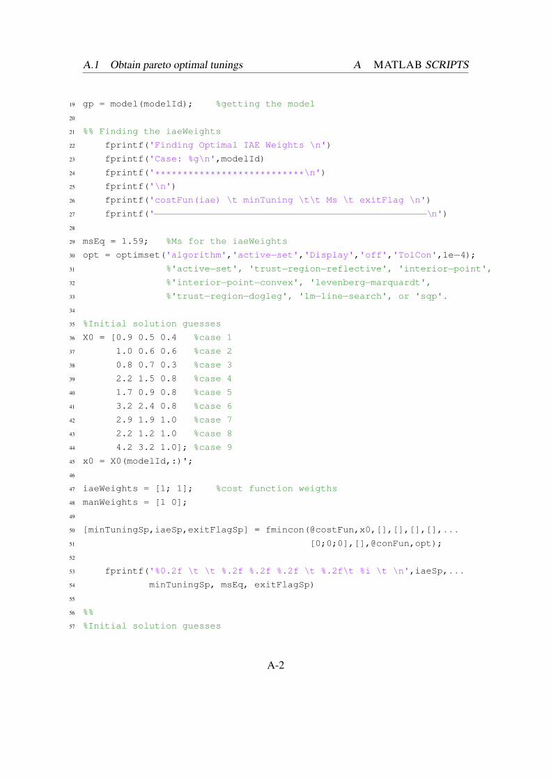
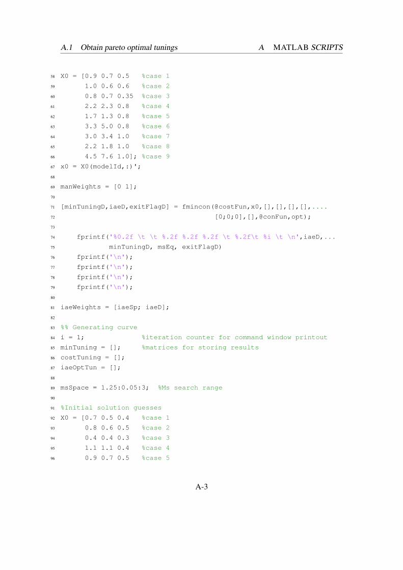
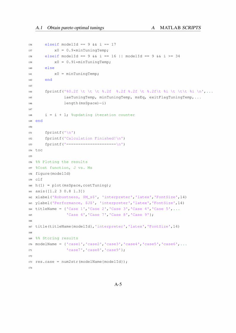
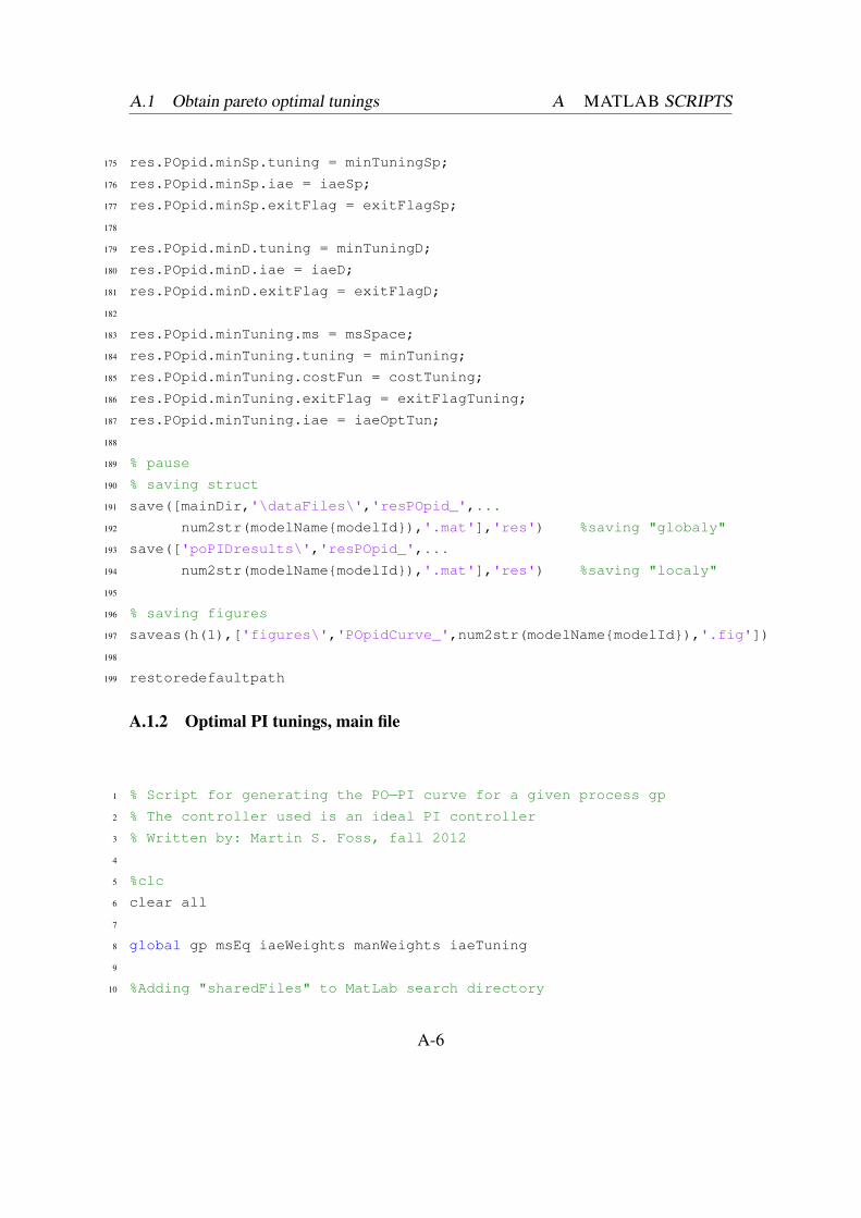
A MATLAB Scripts A-1A.1 Obtain pareto optimal tunings . . . . . . . . . . . . . . . . . . . . . . A-1
iii
TABLE OF CONTENTS TABLE OF CONTENTS
A.1.1 Optimal PID tunings, main file . . . . . . . . . . . . . . . . . . A-1A.1.2 Optimal PI tunings, main file . . . . . . . . . . . . . . . . . . . A-6A.1.3 Cost function . . . . . . . . . . . . . . . . . . . . . . . . . . . A-12A.1.4 Constraints . . . . . . . . . . . . . . . . . . . . . . . . . . . . A-12
A.2 Obtain PO vs. SIMC tuning plots . . . . . . . . . . . . . . . . . . . . . A-12A.2.1 Main file . . . . . . . . . . . . . . . . . . . . . . . . . . . . . A-12A.2.2 Cost function . . . . . . . . . . . . . . . . . . . . . . . . . . . A-20A.2.3 SIMC PI-tunings . . . . . . . . . . . . . . . . . . . . . . . . . A-20A.2.4 SIMC PID-tunings . . . . . . . . . . . . . . . . . . . . . . . . A-21
A.3 Obtain step responses . . . . . . . . . . . . . . . . . . . . . . . . . . . A-23A.3.1 Main file . . . . . . . . . . . . . . . . . . . . . . . . . . . . . A-23
A.4 Obtain parallel tuning parameters . . . . . . . . . . . . . . . . . . . . . A-29A.4.1 Main file . . . . . . . . . . . . . . . . . . . . . . . . . . . . . A-29
A.5 Shared files . . . . . . . . . . . . . . . . . . . . . . . . . . . . . . . . A-31A.5.1 Cases - second order models . . . . . . . . . . . . . . . . . . . A-31A.5.2 Cases - first order models . . . . . . . . . . . . . . . . . . . . . A-32A.5.3 Controller . . . . . . . . . . . . . . . . . . . . . . . . . . . . . A-33A.5.4 Integral absolute error . . . . . . . . . . . . . . . . . . . . . . A-34A.5.5 Ms . . . . . . . . . . . . . . . . . . . . . . . . . . . . . . . . A-35
B SIMULINK Model B-1
iv
LIST OF FIGURES LIST OF FIGURES
List of Figures
2.1 Block diagram of general feedback control system. . . . . . . . . . . . 22.2 Block diagram of feedback control system used in the project. . . . . . 32.3 Typical Pareto-optimal curve of two conflicting objective functions. . . 63.1 PO vs. SIMC, time delay dominated processes. . . . . . . . . . . . . . 13
(a) Case 1, τ2τ1= 0.5, τ2
θ= 0.5. . . . . . . . . . . . . . . . . . . . . . 13
(b) Case 2, τ2τ1= 0.8, τ2
θ= 0.8. . . . . . . . . . . . . . . . . . . . . . 13
(c) Case 3, τ2τ1= 0.3, τ2
θ= 0.3. . . . . . . . . . . . . . . . . . . . . . 13
3.2 PO vs. SIMC, with τ2τ1= 0.5. . . . . . . . . . . . . . . . . . . . . . . . 15
(a) Case 4, τ2θ= 1.5. . . . . . . . . . . . . . . . . . . . . . . . . . . 15
(b) Case 7, τ2θ= 2.0. . . . . . . . . . . . . . . . . . . . . . . . . . . 15
3.3 PO vs. SIMC, with τ2τ1= 0.8. . . . . . . . . . . . . . . . . . . . . . . . 17
(a) Case 5, τ2θ= 1.5. . . . . . . . . . . . . . . . . . . . . . . . . . . 17
(b) Case 8, τ2θ= 2.0. . . . . . . . . . . . . . . . . . . . . . . . . . . 17
3.4 PO vs. SIMC, with τ2τ1= 0.3. . . . . . . . . . . . . . . . . . . . . . . . 19
(a) Case 6, τ2θ= 1.5. . . . . . . . . . . . . . . . . . . . . . . . . . . 19
(b) Case 9, τ2θ= 2.0. . . . . . . . . . . . . . . . . . . . . . . . . . . 19
3.5 Step responses, time delay dominated processes. . . . . . . . . . . . . . 23(a) Case 1, τ2
τ1= 0.5, τ2
θ= 0.5. . . . . . . . . . . . . . . . . . . . . . 23
(b) Case 2, τ2τ1= 0.8, τ2
θ= 0.8. . . . . . . . . . . . . . . . . . . . . . 23
(c) Case 3, τ2τ1= 0.3, τ2
θ= 0.3. . . . . . . . . . . . . . . . . . . . . . 23
3.6 Step responses, with τ2τ1= 0.5. . . . . . . . . . . . . . . . . . . . . . . 25
(a) Case 4, τ2θ= 1.5. . . . . . . . . . . . . . . . . . . . . . . . . . . 25
(b) Case 7, τ2θ= 2.0. . . . . . . . . . . . . . . . . . . . . . . . . . . 25
3.7 Step responses, with τ2τ1= 0.8. . . . . . . . . . . . . . . . . . . . . . . 27
(a) Case 5, τ2θ= 1.5. . . . . . . . . . . . . . . . . . . . . . . . . . . 27
(b) Case 8, τ2θ= 2.0. . . . . . . . . . . . . . . . . . . . . . . . . . . 27
3.8 Step responses, with τ2τ1= 0.3. . . . . . . . . . . . . . . . . . . . . . . 29
(a) Case 6, τ2θ= 1.5. . . . . . . . . . . . . . . . . . . . . . . . . . . 29
(b) Case 9, τ2θ= 2.0. . . . . . . . . . . . . . . . . . . . . . . . . . . 29
B.1 SIMULINK model . . . . . . . . . . . . . . . . . . . . . . . . . . . . . B-1
v

LIST OF TABLES LIST OF TABLES
List of Tables
3.1 Pareto-optimal IAE-weights. . . . . . . . . . . . . . . . . . . . . . . . 113.2 Tuning variables, parallel form. . . . . . . . . . . . . . . . . . . . . . . 21
vi
LIST OF SYMBOLS LIST OF SYMBOLS
List of Symbols
Symbol Explanation
d Disturbance, inputdout Disturbance, output
e Error, controller inputgc Controller model (transfer function)gp Process model (transfer function)
IAE Integral absolute errork Process gain
Kc Controller gainJ Cost function
Ms Peak in sensitivity functionω Frequencys Laplace-variablet Timeτ1 1st time constant (largest)τ2 2nd time constant (smallest)τc Closed loop time constantτD Derivative time constantτI Integral time constantθ Time delayu Process input
vii
1 INTRODUCTION
1 Introduction
One of the most used controllers in the industry is the PID controller [1]. Despitethe frequent use, this type of controller is often poorly tuned. Though there are onlythree tuning parameters in the PID controller the optimal tuning, i.e. optimal trade-offbetween performance and robustness, is difficult to obtain. The optimal performancecan in itself also be difficult to define. The requirements of robustness and performancemay need good engineering insight to be determined. It is not possible to get the best ofboth, so a settlement in the middle ground should be chosen.
The aim of this report is to validate the SIMC tuning rules presented by Skogestad [2].These rules are developed to be easy to remember and to result in good closed-loopbehavior. Earlier investigations that has been preformed to investigate the SIMC tuningrules with respect to PI control [3], has shown that these rules result in good trade-offbetween robustness and performance.
The tuning rules is tested to a set of second-order-plus-time-delay (SOPTD) processes.The performance of the PID controller tunings will be compared with the "Pareto-optimal" (PO) tunings, which can be referred to as "the best one can get". The PIDtunings will also be compared with PI tunings. The latter to see if there is any need ofimplementing a PID controller.
1
2 THEORY - BACKGROUND
2 Theory - Background
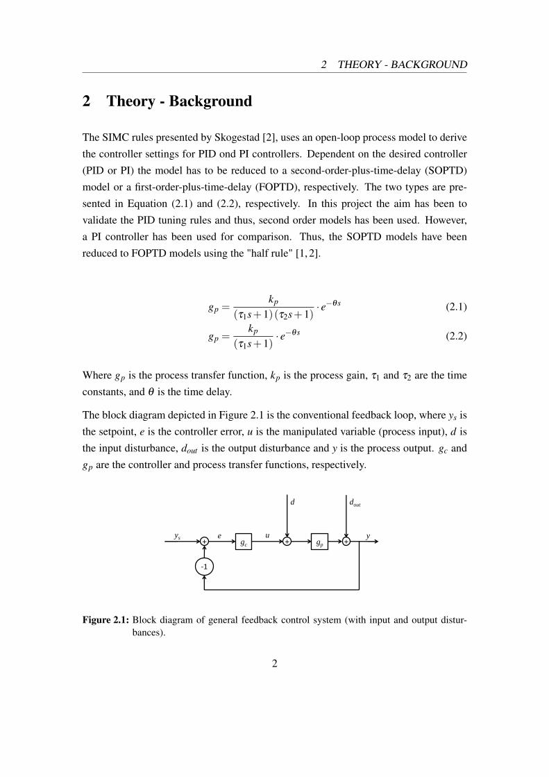
The SIMC rules presented by Skogestad [2], uses an open-loop process model to derivethe controller settings for PID ond PI controllers. Dependent on the desired controller(PID or PI) the model has to be reduced to a second-order-plus-time-delay (SOPTD)model or a first-order-plus-time-delay (FOPTD), respectively. The two types are pre-sented in Equation (2.1) and (2.2), respectively. In this project the aim has been tovalidate the PID tuning rules and thus, second order models has been used. However,a PI controller has been used for comparison. Thus, the SOPTD models have beenreduced to FOPTD models using the "half rule" [1, 2].
gp =kp
(τ1s+1)(τ2s+1)· e−θs (2.1)
gp =kp
(τ1s+1)· e−θs (2.2)
Where gp is the process transfer function, kp is the process gain, τ1 and τ2 are the timeconstants, and θ is the time delay.
The block diagram depicted in Figure 2.1 is the conventional feedback loop, where ys isthe setpoint, e is the controller error, u is the manipulated variable (process input), d isthe input disturbance, dout is the output disturbance and y is the process output. gc andgp are the controller and process transfer functions, respectively.
ys + gp +
-1
d
y u +
dout
e gc
Figure 2.1: Block diagram of general feedback control system (with input and output distur-bances).
2
2.1 The PID controller and SIMC tuning rules 2 THEORY - BACKGROUND
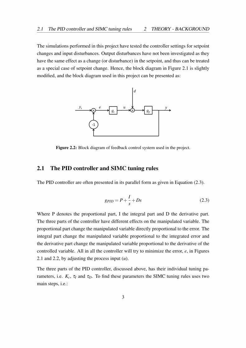
The simulations performed in this project have tested the controller settings for setpointchanges and input disturbances. Output disturbances have not been investigated as theyhave the same effect as a change (or disturbance) in the setpoint, and thus can be treatedas a special case of setpoint change. Hence, the block diagram in Figure 2.1 is slightlymodified, and the block diagram used in this project can be presented as:
ys + gp +
-1
d
y u e gc
Figure 2.2: Block diagram of feedback control system used in the project.
2.1 The PID controller and SIMC tuning rules
The PID controller are often presented in its parallel form as given in Equation (2.3).
gPID = P+Is+Ds (2.3)
Where P denotes the proportional part, I the integral part and D the derivative part.The three parts of the controller have different effects on the manipulated variable. Theproportional part change the manipulated variable directly proportional to the error. Theintegral part change the manipulated variable proportional to the integrated error andthe derivative part change the manipulated variable proportional to the derivative of thecontrolled variable. All in all the controller will try to minimize the error, e, in Figures2.1 and 2.2, by adjusting the process input (u).
The three parts of the PID controller, discussed above, has their individual tuning pa-rameters, i.e. Kc, τI and τD. To find these parameters the SIMC tuning rules uses twomain steps, i.e.:
3
2.1 The PID controller and SIMC tuning rules 2 THEORY - BACKGROUND
1. Obtain a FOPTD or a SOPTD model.
• Perform open or closed loop experiments.
• If model of higher order is known, reduce with use of the "half rule".
2. Get controller settings from the tuning rules, presented below.
The SIMC tuning rules are given for the ideal, series form, PID controller, as defined inEquation (2.4).
gc(s) = Kc ·(
τIs+1τIs
)· (τDs+1) (2.4)
Where gc is the controller transfer function, Kc is the controller gain, τI is the integraltime and τD is the derivative time. The tuning rules [2] for a PID controller can be foundfrom a SOPTD process, see Equation (2.1), as follows:
Kc =1k
τ1
τc +θ(2.5)
τI = min{τ1,4(τc +θ)} (2.6)
τD = τ2 (2.7)
As seen from Equation (2.5) - (2.7) the SIMC tuning rules has only one independentvariable, i.e. τc. The recommended value for this parameter is τc = θ , which shouldyield tight control with good trade-off between robustness and performance.
If a PI controller is to be tuned, the Kc and τI parameter are defined in the same manner.τD = 0, as the PI controller do not have this tuning parameter.
As the PID controller often is presented in its parallell form, Equation (2.8), recalcula-tion of the tuning parameters are required. The corresponding parallell tuning param-eters can be calculated by the translation formulas presented in Equations (2.9), (2.10)and (2.11).
4

2.2 Pareto optimization 2 THEORY - BACKGROUND
g′c(s) = K′c
(1+
1τ ′Is
+ τ′Ds)
(2.8)
K′c = Kc
(1+
τD
τI
)(2.9)
τ′I = τI
(1+
τD
τI
)(2.10)
τ′D =
τD
1+τD
τI
(2.11)
Where g′c, K′c, τ ′I and τ ′D are the parallel controller transfer function, controller gain,integral time and derivative time, respectively.
2.2 Pareto optimization
The search after good controller tunings can be difficult without a systematic approach.A set of tuning parameters can never yield perfect performance and good robustness atthe same time. A controller with good performance is normally not very robust, andvice versa. There will also be a trade-off between the response to a change in setpointand disturbances.
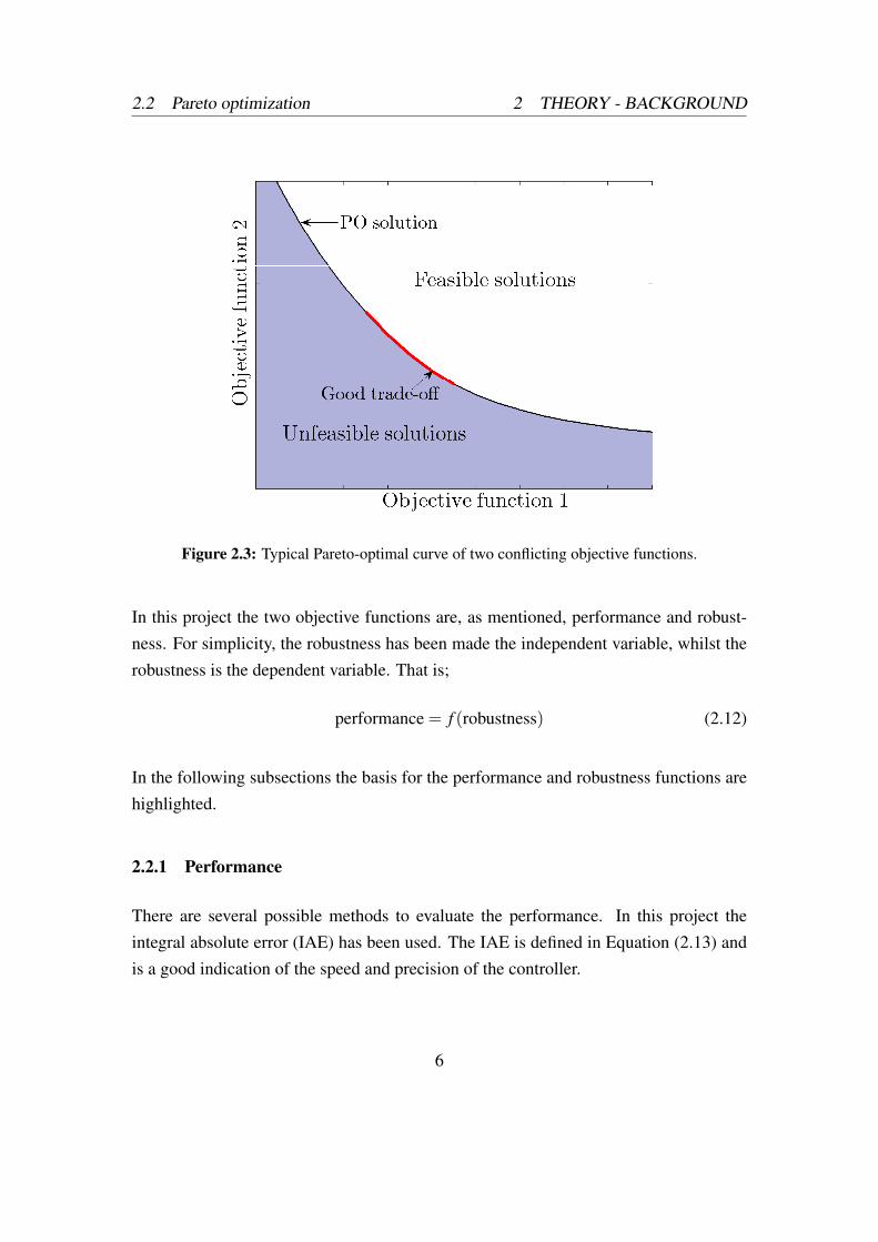
To be able to find the optimal compromise between performance and robustness Pareto-optimal (PO) curves can be helpful. A PO-curve is represented in Figure 2.3. The figuredepicts two conflicting objective functions plotted against each other. For each point,the optimal value of the two objective functions are plotted. The trade-off is clearlydepicted. As objective function 1 is low, objective function 2 is high, and vice versa.The optimal point is somewhere in the middle (bold, red line), but exactly where is upto the individual engineer and the respective case.
5
2.2 Pareto optimization 2 THEORY - BACKGROUND
Figure 2.3: Typical Pareto-optimal curve of two conflicting objective functions.
In this project the two objective functions are, as mentioned, performance and robust-ness. For simplicity, the robustness has been made the independent variable, whilst therobustness is the dependent variable. That is;
performance = f (robustness) (2.12)
In the following subsections the basis for the performance and robustness functions arehighlighted.
2.2.1 Performance
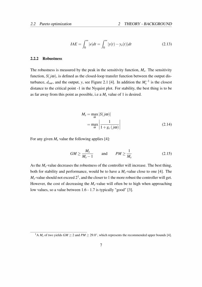
There are several possible methods to evaluate the performance. In this project theintegral absolute error (IAE) has been used. The IAE is defined in Equation (2.13) andis a good indication of the speed and precision of the controller.
6
2.2 Pareto optimization 2 THEORY - BACKGROUND
IAE =∫
∞
0|e|dt =
∫∞
0|y(t)− ys(t)|dt (2.13)
2.2.2 Robustness
The robustness is measured by the peak in the sensitivity function, Ms. The sensitivityfunction, S( jω), is defined as the closed-loop transfer function between the output dis-turbance, dout , and the output, y, see Figure 2.1 [4]. In addition the M−1
s is the closestdistance to the critical point -1 in the Nyquist plot. For stability, the best thing is to beas far away from this point as possible, i.e a Ms value of 1 is desired.
Ms = maxω|S( jω)|
= maxω
∣∣∣∣ 11+gc ( jω)
∣∣∣∣ (2.14)
For any given Ms value the following applies [4]:
GM ≥ Ms
Ms−1and PM ≥ 1
Ms(2.15)
As the Ms-value decreases the robustness of the controller will increase. The best thing,both for stability and performance, would be to have a Ms-value close to one [4]. TheMs-value should not exceed 21, and the closer to 1 the more robust the controller will get.However, the cost of decreasing the Ms-value will often be to high when approachinglow values, so a value between 1.6 - 1.7 is typically "good" [3].
1A Ms of two yields GM ≥ 2 and PM ≥ 29.0◦, which represents the recommended upper bounds [4].
7

2.3 The objective function 2 THEORY - BACKGROUND
2.3 The objective function
The objective function, which should be minimized, used in this project is defined byEquation (2.16). The function has been calculated in the domain given in Equation(2.17).
J(c) = 0.5
[IAEys(c)
IAE◦ys+
IAEd(c)IAE◦d
](2.16)
Ms = {1.25,1.30, . . . ,3.00} (2.17)
Where IAE◦ys and IAE◦d denotes the error when there is performed an input and a dis-turbance step with a Pareto-optimal tuning, respectively. In this way the performanceis weighted against a constant reference. As the performance is a function of the ro-bustness, a Ms-value of 1.59 is used when the PO-curves are constructed. The resultingweights are presented in Table 3.1.
2.4 Cases
In this project nine cases have been tested. These are given in Equation (2.18) – (2.23).The first three cases, case 1 – case 3, are time delay dominated processes, whilst case 4– case 9 are lag dominated.
Case 1:gp =
1(s+1)(0.5s+1)
· e(−s) (2.18)
Case 2:gp =
1(s+1)(0.8s+1)
· e(−s) (2.19)
Case 3:gp =
1(s+1)(0.3s+1)
· e(−s) (2.20)
8
2.5 Calculations and Simulations 2 THEORY - BACKGROUND
Case 4:gp =
1(s+1)(0.5s+1)
· e(−13 s) (2.21)
Case 5:gp =
1(s+1)(0.8s+1)
· e(−815 s) (2.22)
Case 6:gp =
1(s+1)(0.3s+1)
· e(−215 s) (2.23)
Case 7:gp =
1(s+1)(0.5s+1)
· e(−0.25s) (2.24)
Case 8:gp =
1(s+1)(0.8s+1)
· e(−0.4s) (2.25)
Case 9:gp =
1(s+1)(0.3s+1)
· e(−0.1s) (2.26)
2.5 Calculations and Simulations
All calculations and simulations in this project are performed by use of MATLAB andSIMULINK. The MATLAB scripts and SIMULINK block diagram are included in Ap-pendix A and B, respectively.
9
3 RESULTS AND DISCUSSION
3 Results and Discussion
In the following sections all the obtained results are presented along with a discussion.
3.1 Pareto-optimal PID and PI weights
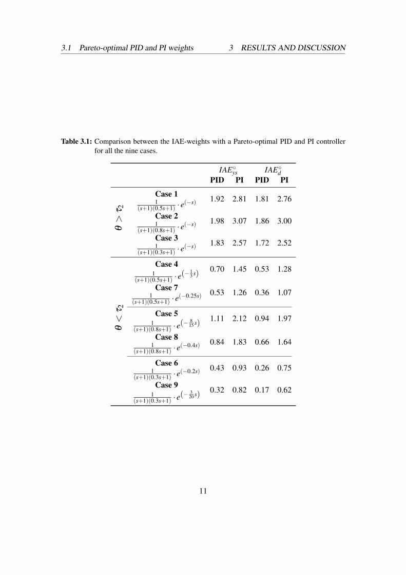
To be able to assess the performance of the controllers for the different cases the costfunction in Equation (2.16) had to be solved. In order to achieve this, the IAE◦ys andIAE◦d had to be calculated. This was performed by calculating the error with only a stepchange in the setpoint and disturbance, respectively. These Pareto-optimal parameterswas found for both the PID and a PI controllers for a Ms-value of 1.59. All the theweights are presented in Table 3.1.
As can be seen from Table 3.1 there is a consistently better performance by the PIDcontroller, both for setpoint changes and disturbances, for all cases. This observationfits well with theory, as the PID controller has one extra tuning parameter comparedwith the PI controller, and should therefore perform better. The PO-controllers are alsoobserved to perform better to disturbances than to a step in the setpoint.
10
3.1 Pareto-optimal PID and PI weights 3 RESULTS AND DISCUSSION
Table 3.1: Comparison between the IAE-weights with a Pareto-optimal PID and PI controllerfor all the nine cases.
IAE◦ys IAE◦dPID PI PID PI
θ>
τ2
Case 11.92 2.81 1.81 2.761
(s+1)(0.5s+1) · e(−s)
Case 21.98 3.07 1.86 3.001
(s+1)(0.8s+1) · e(−s)
Case 31.83 2.57 1.72 2.521
(s+1)(0.3s+1) · e(−s)
θ<
τ2
Case 40.70 1.45 0.53 1.28
1(s+1)(0.5s+1) · e
(− 13 s)
Case 70.53 1.26 0.36 1.071
(s+1)(0.5s+1) · e(−0.25s)
Case 51.11 2.12 0.94 1.97
1(s+1)(0.8s+1) · e
(− 815 s)
Case 80.84 1.83 0.66 1.641
(s+1)(0.8s+1) · e(−0.4s)
Case 60.43 0.93 0.26 0.751
(s+1)(0.3s+1) · e(−0.2s)
Case 90.32 0.82 0.17 0.62
1(s+1)(0.3s+1) · e
(− 320 s)
11
3.2 Pareto-optimal vs. SIMC tunings 3 RESULTS AND DISCUSSION
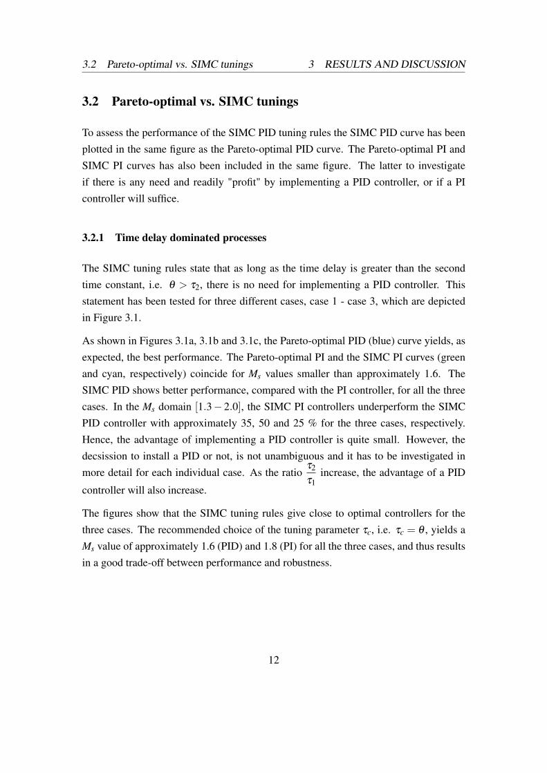
3.2 Pareto-optimal vs. SIMC tunings
To assess the performance of the SIMC PID tuning rules the SIMC PID curve has beenplotted in the same figure as the Pareto-optimal PID curve. The Pareto-optimal PI andSIMC PI curves has also been included in the same figure. The latter to investigateif there is any need and readily "profit" by implementing a PID controller, or if a PIcontroller will suffice.
3.2.1 Time delay dominated processes
The SIMC tuning rules state that as long as the time delay is greater than the secondtime constant, i.e. θ > τ2, there is no need for implementing a PID controller. Thisstatement has been tested for three different cases, case 1 - case 3, which are depictedin Figure 3.1.
As shown in Figures 3.1a, 3.1b and 3.1c, the Pareto-optimal PID (blue) curve yields, asexpected, the best performance. The Pareto-optimal PI and the SIMC PI curves (greenand cyan, respectively) coincide for Ms values smaller than approximately 1.6. TheSIMC PID shows better performance, compared with the PI controller, for all the threecases. In the Ms domain [1.3− 2.0], the SIMC PI controllers underperform the SIMCPID controller with approximately 35, 50 and 25 % for the three cases, respectively.Hence, the advantage of implementing a PID controller is quite small. However, thedecsission to install a PID or not, is not unambiguous and it has to be investigated inmore detail for each individual case. As the ratio
τ2
τ1increase, the advantage of a PID
controller will also increase.
The figures show that the SIMC tuning rules give close to optimal controllers for thethree cases. The recommended choice of the tuning parameter τc, i.e. τc = θ , yields aMs value of approximately 1.6 (PID) and 1.8 (PI) for all the three cases, and thus resultsin a good trade-off between performance and robustness.
12
3.2 Pareto-optimal vs. SIMC tunings 3 RESULTS AND DISCUSSION
Robustness, Ms
Perform
ance,J(c)
1 1.5 2 2.5 3
1
2
3
4
5
6
7
8
τ2
τ1= 0.5
τ2
θ= 0.5
τc = 0.5θ
τc = θ
τc = 1.5θ
PO (PID)
PO (PI)
SIMC (PID)
SIMC(PI)
(a) Case 1, τ2τ1
= 0.5, τ2θ= 0.5.
Robustness, Ms
Perform
ance,J(c)
1 1.5 2 2.5 3
1
2
3
4
5
6
7
8
τ2
τ1= 0.8
τ2
θ= 0.8
τc = 0.5θ
τc = θ
τc = 1.5θ
PO (PID)
PO (PI)
SIMC (PID)
SIMC(PI)
(b) Case 2, τ2τ1
= 0.8, τ2θ= 0.8.
Robustness, Ms
Perform
ance,J(c)
1 1.5 2 2.5 3
1
2
3
4
5
6
7
8
τ2
τ1= 0.3
τ2
θ= 0.3
τc = 0.5θ
τc = θ
τc = 1.5θ
PO (PID)
PO (PI)
SIMC (PID)
SIMC(PI)
(c) Case 3, τ2τ1
= 0.3, τ2θ= 0.3.
Figure 3.1: Pareto optimal (PO) vs. SIMC tuning curves for time delay dominated second orderplus time delay processes on the form gp =
1(τ1s+1)(τ2s+1) · exp(−θs).
13
3.2 Pareto-optimal vs. SIMC tunings 3 RESULTS AND DISCUSSION
3.2.2 Lag dominated processes
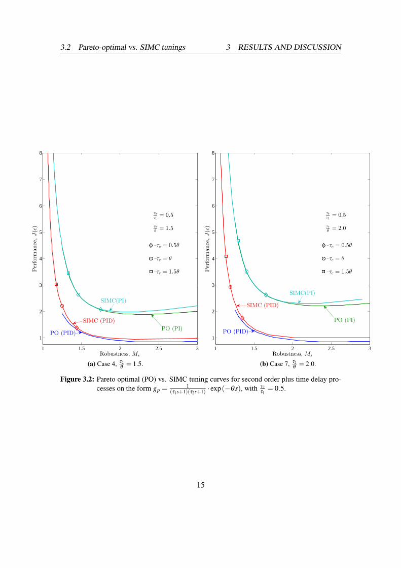
The remaining cases has been plotted in the same manner as the time delay dominatedprocesses, i.e. by comparing the Pareto-optimal PID and PI tuning curves with theSIMC PID and PI tuning curves. The results are presented in Figures 3.2 – 3.4.
Figure 3.2a and 3.2b depicts case 4 and case 7, respectively. In both these cases theratio
τ2
τ1is kept constant at 0.5, whilst the ratio
τ2
θis 1.5 and 2.0, respectively. For both
processes the SIMC tuning rules produces controllers with almost no non-optimalityloss in the preferred Ms domain, i.e. Ms < 2.0. As Ms decreases and approach one, thecost function increases dramatically.
In the Ms domain [1.3−2.0] the SIMC PI underperform the SIMC PID on average withapproximately 105 % for case 4 and and 125 % for case 7.
The figures show that increasing the ratioτ2
θwill result in a shift towards lower Ms
values for given τc’s. The recommended choice of τc = θ is shown to result in a Ms
value of 1.25 for case 4 and 1.20 for case 7. This will give a robust controller, butbecause of the trade-off between performance and robustness, the controller will looseperformance. The steep gradients in these points indicate that by increasing the Ms
value a small amount, will give a large advantage/increase in performance. A τc equalto 0.5 · θ , diamond shaped point in the figures, would be a better alternative for bothprocesses. This tuning parameter will give a Ms-value of 1.44 and 1.35 for the twocases, respectively.
14
3.2 Pareto-optimal vs. SIMC tunings 3 RESULTS AND DISCUSSION
Robustness, Ms
Perform
ance,J(c)
1 1.5 2 2.5 3
1
2
3
4
5
6
7
8
τ2
τ1= 0.5
τ2
θ= 1.5
τc = 0.5θ
τc = θ
τc = 1.5θ
PO (PID)PO (PI)
SIMC (PID)
SIMC(PI)
(a) Case 4, τ2θ= 1.5.
Robustness, Ms
Perform
ance,J(c)
1 1.5 2 2.5 3
1
2
3
4
5
6
7
8
τ2
τ1= 0.5
τ2
θ= 2.0
τc = 0.5θ
τc = θ
τc = 1.5θ
PO (PID)
PO (PI)
SIMC (PID)
SIMC(PI)
(b) Case 7, τ2θ= 2.0.
Figure 3.2: Pareto optimal (PO) vs. SIMC tuning curves for second order plus time delay pro-cesses on the form gp =
1(τ1s+1)(τ2s+1) · exp(−θs), with τ2
τ1= 0.5.
15

3.2 Pareto-optimal vs. SIMC tunings 3 RESULTS AND DISCUSSION
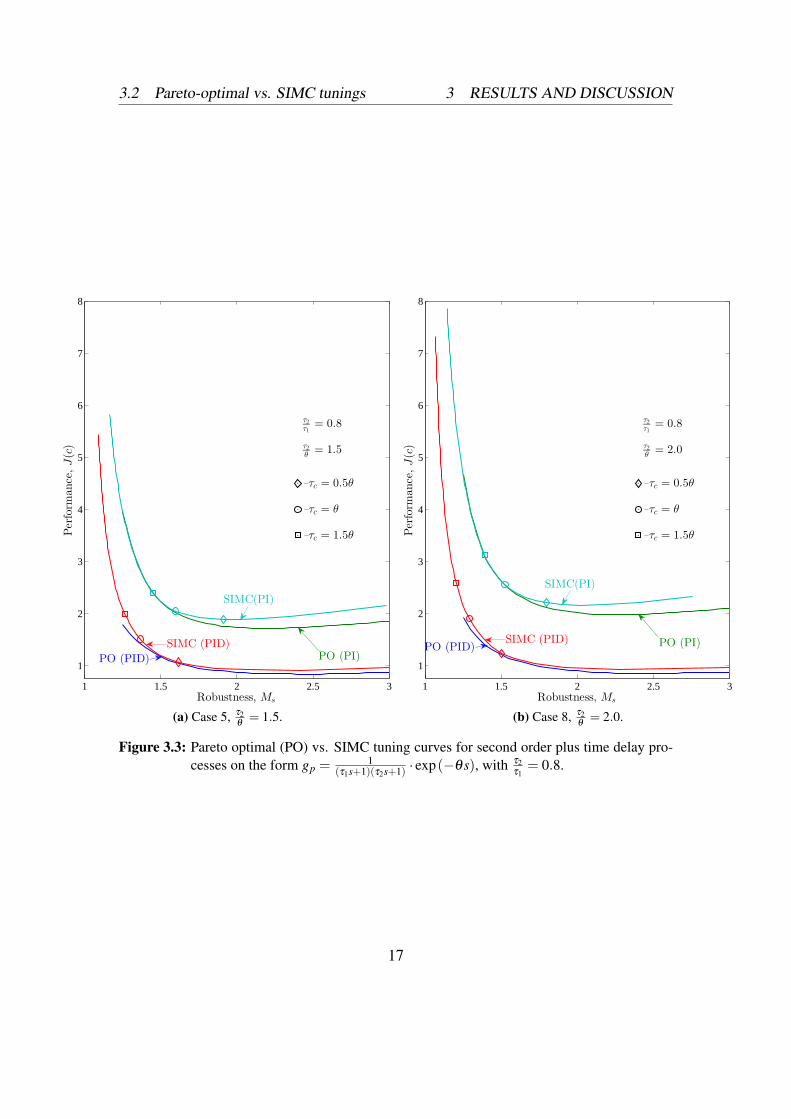
Figure 3.3a and 3.3b depicts case 5 and case 8, respectively. In both these cases theratio
τ2
τ1is kept constant at 0.8, whilst the ratio
τ2
θis 1.5 and 2.0, respectively. For both
processes the SIMC tuning rules produces controllers with almost no non-optimalityloss in the preferred Ms domain, i.e. Ms < 2.0. As Ms decreases and approach one, thecost function increases dramatically.
In the Ms domain [1.3−2.0] the SIMC PI underperform the SIMC PID on average withapproximately 95 % for case 5 and 120 % for case 8.
The figures show that increasing the ratioτ2
θwill result in a shift towards lower Ms
values for given τc’s. The recommended choice of τc = θ is shown to result in a Ms
value of 1.37 for case 5 and 1.29 for case 8. These tunings give a good trade-off betweenperformance and robustness. If the tuning parameter, τc, was selected to 0.5 ·θ , diamondshaped point in the figures, the resulting Ms values would be 1.62 and 1.50 for the twocases, respectively. These values will also result in a decent trade-off.
16
3.2 Pareto-optimal vs. SIMC tunings 3 RESULTS AND DISCUSSION
Robustness, Ms
Perform
ance,J(c)
1 1.5 2 2.5 3
1
2
3
4
5
6
7
8
τ2
τ1= 0.8
τ2
θ= 1.5
τc = 0.5θ
τc = θ
τc = 1.5θ
PO (PID) PO (PI)SIMC (PID)
SIMC(PI)
(a) Case 5, τ2θ= 1.5.
Robustness, Ms
Perform
ance,J(c)
1 1.5 2 2.5 3
1
2
3
4
5
6
7
8
τ2
τ1= 0.8
τ2
θ= 2.0
τc = 0.5θ
τc = θ
τc = 1.5θ
PO (PID) PO (PI)SIMC (PID)
SIMC(PI)
(b) Case 8, τ2θ= 2.0.
Figure 3.3: Pareto optimal (PO) vs. SIMC tuning curves for second order plus time delay pro-cesses on the form gp =
1(τ1s+1)(τ2s+1) · exp(−θs), with τ2
τ1= 0.8.
17
3.2 Pareto-optimal vs. SIMC tunings 3 RESULTS AND DISCUSSION
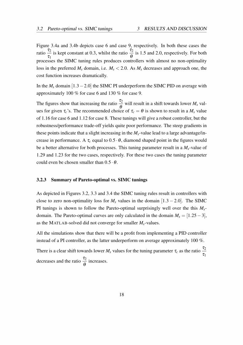
Figure 3.4a and 3.4b depicts case 6 and case 9, respectively. In both these cases theratio
τ2
τ1is kept constant at 0.3, whilst the ratio
τ2
θis 1.5 and 2.0, respectively. For both
processes the SIMC tuning rules produces controllers with almost no non-optimalityloss in the preferred Ms domain, i.e. Ms < 2.0. As Ms decreases and approach one, thecost function increases dramatically.
In the Ms domain [1.3−2.0] the SIMC PI underperform the SIMC PID on average withapproximately 100 % for case 6 and 130 % for case 9.
The figures show that increasing the ratioτ2
θwill result in a shift towards lower Ms val-
ues for given τc’s. The recommended choice of τc = θ is shown to result in a Ms valueof 1.16 for case 6 and 1.12 for case 8. These tunings will give a robust controller, but therobustness/performance trade-off yields quite poor performance. The steep gradients inthese points indicate that a slight increasing in the Ms-value lead to a large advantage/in-crease in performance. A τc equal to 0.5 ·θ , diamond shaped point in the figures wouldbe a better alternative for both processes. This tuning parameter result in a Ms-value of1.29 and 1.23 for the two cases, respectively. For these two cases the tuning parametercould even be chosen smaller than 0.5 ·θ .
3.2.3 Summary of Pareto-optimal vs. SIMC tunings
As depicted in Figures 3.2, 3.3 and 3.4 the SIMC tuning rules result in controllers withclose to zero non-optimality loss for Ms values in the domain [1.3− 2.0]. The SIMCPI tunings is shown to follow the Pareto-optimal surprisingly well over the this Ms-domain. The Pareto-optimal curves are only calculated in the domain Ms = [1.25−3],as the MATLAB-solved did not converge for smaller Ms-values.
All the simulations show that there will be a profit from implementing a PID controllerinstead of a PI controller, as the latter underperform on average approximately 100 %.
There is a clear shift towards lower Ms values for the tuning parameter τc as the ratioτ2
τ1
decreases and the ratioτ2
θincreases.
18
3.2 Pareto-optimal vs. SIMC tunings 3 RESULTS AND DISCUSSION
Robustness, Ms
Perform
ance,J(c)
1 1.5 2 2.5 3
1
2
3
4
5
6
7
8
τ2
τ1= 0.3
τ2
θ= 1.5
τc = 0.5θ
τc = θ
τc = 1.5θ
PO (PID)PO (PI)
SIMC (PID)
SIMC(PI)
(a) Case 6, τ2θ= 1.5.
Robustness, Ms
Perform
ance,J(c)
1 1.5 2 2.5 3
1
2
3
4
5
6
7
8
τ2
τ1= 0.3
τ2
θ= 2.0
τc = 0.5θ
τc = θ
τc = 1.5θ
PO (PID)
PO (PI)SIMC (PID)
SIMC(PI)
(b) Case 9, τ2θ= 2.0.
Figure 3.4: Pareto optimal (PO) vs. SIMC tuning curves for second order plus time delay pro-cesses on the form gp =
1(τ1s+1)(τ2s+1) · exp(−θs), with τ2
τ1= 0.3.
19

3.3 Step responses 3 RESULTS AND DISCUSSION
3.3 Step responses
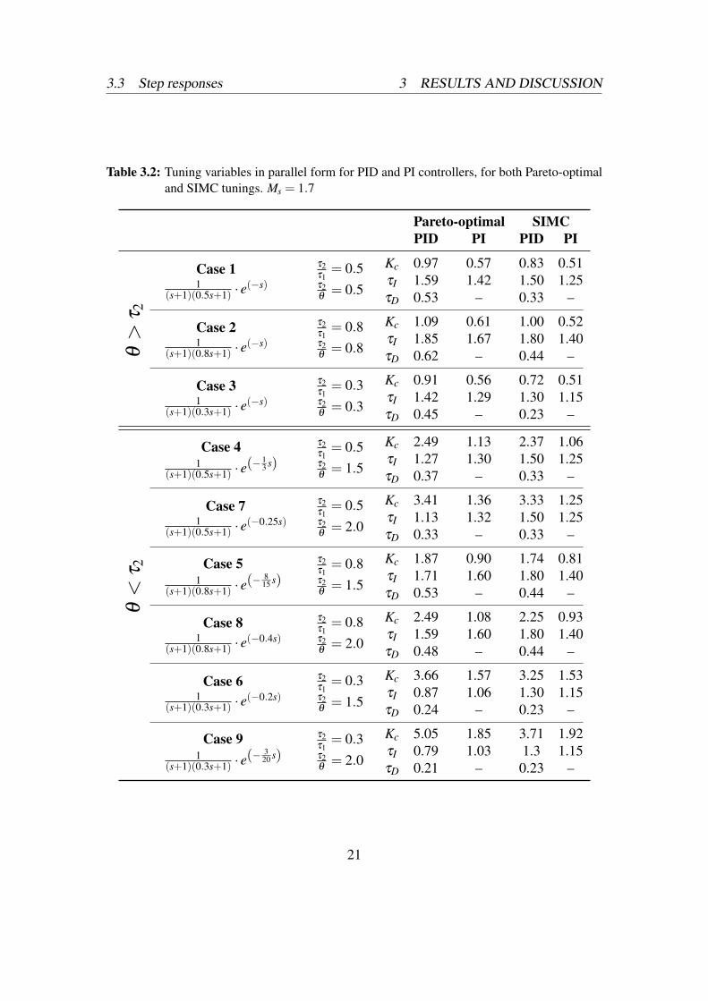
The Pareto-optimal and SIMC tunings has been tested by performing step changesin setpoint and input disturbance. The SIMULINK block diagram is included in Ap-pendix A. The controller tunings used corresponds to a Ms value of 1.7. All the tuningvariables, in parallel form, used for the step response experiments are presented in Ta-ble 3.2.
In the subsequent sections the step response experiments for the different cases arepresented by the use of plots of the output, y, and input, u, as functions of time, t.
20
3.3 Step responses 3 RESULTS AND DISCUSSION
Table 3.2: Tuning variables in parallel form for PID and PI controllers, for both Pareto-optimaland SIMC tunings. Ms = 1.7
Pareto-optimal SIMCPID PI PID PI
θ>
τ2
Case 11
(s+1)(0.5s+1) · e(−s)
τ2τ1= 0.5
τ2θ= 0.5
Kc 0.97 0.57 0.83 0.51τI 1.59 1.42 1.50 1.25τD 0.53 – 0.33 –
Case 21
(s+1)(0.8s+1) · e(−s)
τ2τ1= 0.8
τ2θ= 0.8
Kc 1.09 0.61 1.00 0.52τI 1.85 1.67 1.80 1.40τD 0.62 – 0.44 –
Case 31
(s+1)(0.3s+1) · e(−s)
τ2τ1= 0.3
τ2θ= 0.3
Kc 0.91 0.56 0.72 0.51τI 1.42 1.29 1.30 1.15τD 0.45 – 0.23 –
θ<
τ2
Case 41
(s+1)(0.5s+1) · e(− 1
3 s)
τ2τ1= 0.5
τ2θ= 1.5
Kc 2.49 1.13 2.37 1.06τI 1.27 1.30 1.50 1.25τD 0.37 – 0.33 –
Case 71
(s+1)(0.5s+1) · e(−0.25s)
τ2τ1= 0.5
τ2θ= 2.0
Kc 3.41 1.36 3.33 1.25τI 1.13 1.32 1.50 1.25τD 0.33 – 0.33 –
Case 51
(s+1)(0.8s+1) · e(− 8
15 s)
τ2τ1= 0.8
τ2θ= 1.5
Kc 1.87 0.90 1.74 0.81τI 1.71 1.60 1.80 1.40τD 0.53 – 0.44 –
Case 81
(s+1)(0.8s+1) · e(−0.4s)
τ2τ1= 0.8
τ2θ= 2.0
Kc 2.49 1.08 2.25 0.93τI 1.59 1.60 1.80 1.40τD 0.48 – 0.44 –
Case 61
(s+1)(0.3s+1) · e(−0.2s)
τ2τ1= 0.3
τ2θ= 1.5
Kc 3.66 1.57 3.25 1.53τI 0.87 1.06 1.30 1.15τD 0.24 – 0.23 –
Case 91
(s+1)(0.3s+1) · e(− 3
20 s)
τ2τ1= 0.3
τ2θ= 2.0
Kc 5.05 1.85 3.71 1.92τI 0.79 1.03 1.3 1.15τD 0.21 – 0.23 –
21
3.3 Step responses 3 RESULTS AND DISCUSSION
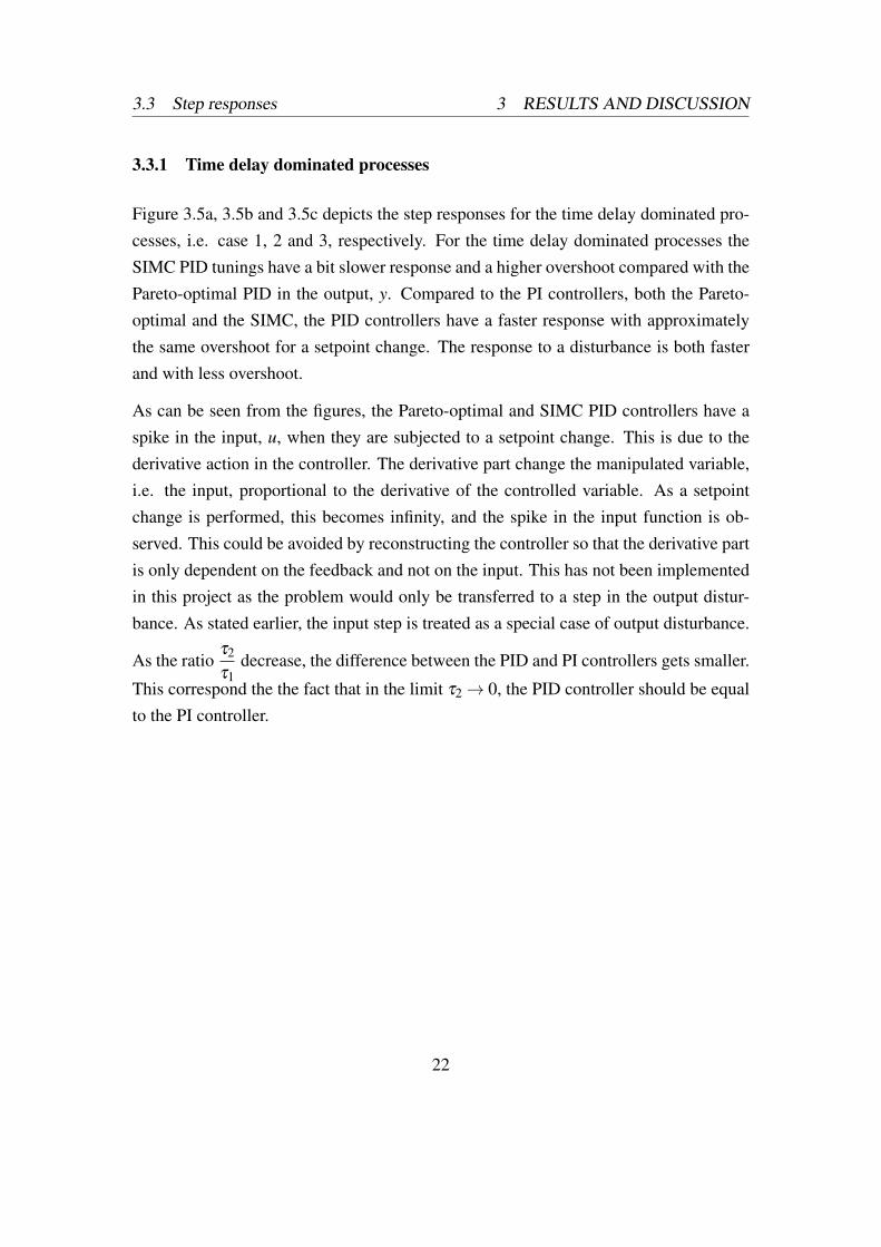
3.3.1 Time delay dominated processes
Figure 3.5a, 3.5b and 3.5c depicts the step responses for the time delay dominated pro-cesses, i.e. case 1, 2 and 3, respectively. For the time delay dominated processes theSIMC PID tunings have a bit slower response and a higher overshoot compared with thePareto-optimal PID in the output, y. Compared to the PI controllers, both the Pareto-optimal and the SIMC, the PID controllers have a faster response with approximatelythe same overshoot for a setpoint change. The response to a disturbance is both fasterand with less overshoot.
As can be seen from the figures, the Pareto-optimal and SIMC PID controllers have aspike in the input, u, when they are subjected to a setpoint change. This is due to thederivative action in the controller. The derivative part change the manipulated variable,i.e. the input, proportional to the derivative of the controlled variable. As a setpointchange is performed, this becomes infinity, and the spike in the input function is ob-served. This could be avoided by reconstructing the controller so that the derivative partis only dependent on the feedback and not on the input. This has not been implementedin this project as the problem would only be transferred to a step in the output distur-bance. As stated earlier, the input step is treated as a special case of output disturbance.
As the ratioτ2
τ1decrease, the difference between the PID and PI controllers gets smaller.
This correspond the the fact that in the limit τ2→ 0, the PID controller should be equalto the PI controller.
22
3.3 Step responses 3 RESULTS AND DISCUSSION
0 5 10 15 20 25 30 35 400
0.5
1
1.5
2
Outp
ut,
y
0 5 10 15 20 25 30 35 40
0
1
2
3
4
Input,
u
Time, t
Ms = 1.7 τ2
τ1= 0.5
τ2
θ= 0.5-- setpoint
PO (PID)
PO (PI)SIMC (PID)
SIMC(PI)
PO (PID)PO (PI) SIMC (PID)
SIMC(PI)
(a) Case 1, τ2τ1
= 0.5, τ2θ= 0.5.
0 5 10 15 20 25 30 35 400
0.5
1
1.5
2
Outp
ut,
y
0 5 10 15 20 25 30 35 40
0
1
2
3
4
Input,
u
Time, t
Ms = 1.7 τ2
τ1= 0.8
τ2
θ= 0.8-- setpoint
PO (PID)
PO (PI)
SIMC (PID)
SIMC(PI)
PO (PID)PO (PI)
SIMC (PID)
SIMC(PI)
(b) Case 2, τ2τ1
= 0.8, τ2θ= 0.8.
0 5 10 15 20 25 30 35 400
0.5
1
1.5
2
Output,
y
0 5 10 15 20 25 30 35 40
0
1
2
3
4
Input,
u
Time, t
Ms = 1.7 τ2
τ1= 0.3
τ2
θ= 0.3-- setpoint
PO (PID)
PO (PI)SIMC (PID)
PO (PID)PO (PI) SIMC (PID)
SIMC(PI)
SIMC(PI)
(c) Case 3, τ2τ1
= 0.3, τ2θ= 0.3.
Figure 3.5: Step responses for time delay dominated second order plus time delay processes onthe form gp =
1(τ1s+1)(τ2s+1) · exp(−θs).
23
3.3 Step responses 3 RESULTS AND DISCUSSION
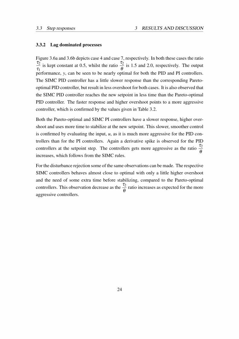
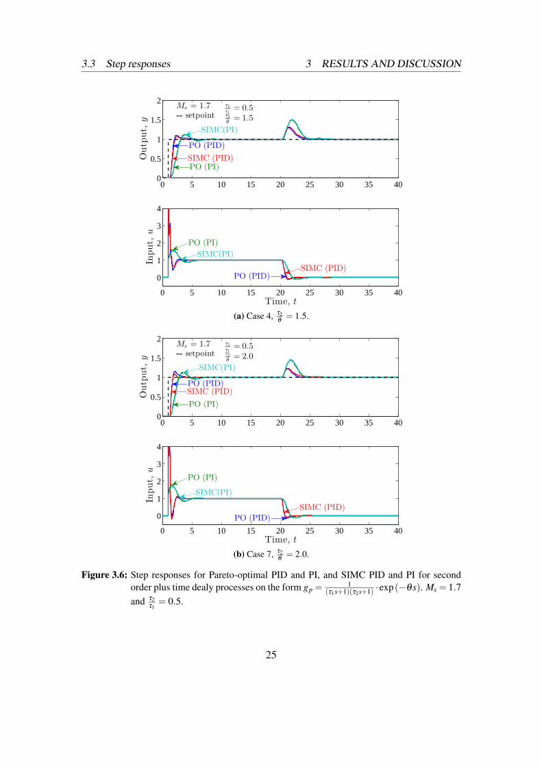
3.3.2 Lag dominated processes
Figure 3.6a and 3.6b depicts case 4 and case 7, respectively. In both these cases the ratioτ2
τ1is kept constant at 0.5, whilst the ratio
τ2
θis 1.5 and 2.0, respectively. The output
performance, y, can be seen to be nearly optimal for both the PID and PI controllers.The SIMC PID controller has a little slower response than the corresponding Pareto-optimal PID controller, but result in less overshoot for both cases. It is also observed thatthe SIMC PID controller reaches the new setpoint in less time than the Pareto-optimalPID controller. The faster response and higher overshoot points to a more aggressivecontroller, which is confirmed by the values given in Table 3.2.
Both the Pareto-optimal and SIMC PI controllers have a slower response, higher over-shoot and uses more time to stabilize at the new setpoint. This slower, smoother controlis confirmed by evaluating the input, u, as it is much more aggressive for the PID con-trollers than for the PI controllers. Again a derivative spike is observed for the PIDcontrollers at the setpoint step. The controllers gets more aggressive as the ratio
τ2
θincreases, which follows from the SIMC rules.
For the disturbance rejection some of the same observations can be made. The respectiveSIMC controllers behaves almost close to optimal with only a little higher overshootand the need of some extra time before stabilizing, compared to the Pareto-optimalcontrollers. This observation decrease as the
τ2
θratio increases as expected for the more
aggressive controllers.
24
3.3 Step responses 3 RESULTS AND DISCUSSION
0 5 10 15 20 25 30 35 400
0.5
1
1.5
2
Output,
y
0 5 10 15 20 25 30 35 40
0
1
2
3
4
Input,
u
Time, t
Ms = 1.7 τ2
τ1= 0.5
τ2
θ= 1.5-- setpoint
PO (PID)
PO (PI)SIMC (PID)
SIMC(PI)
PO (PID)
PO (PI)
SIMC (PID)
SIMC(PI)
(a) Case 4, τ2θ= 1.5.
0 5 10 15 20 25 30 35 400
0.5
1
1.5
2
Output,
y
0 5 10 15 20 25 30 35 40
0
1
2
3
4
Input,
u
Time, t
Ms = 1.7 τ2
τ1= 0.5
τ2
θ= 2.0-- setpoint
PO (PID)
PO (PI)
SIMC (PID)
SIMC(PI)
PO (PID)
PO (PI)
SIMC (PID)
SIMC(PI)
(b) Case 7, τ2θ= 2.0.
Figure 3.6: Step responses for Pareto-optimal PID and PI, and SIMC PID and PI for secondorder plus time dealy processes on the form gp =
1(τ1s+1)(τ2s+1) ·exp(−θs). Ms = 1.7
and τ2τ1= 0.5.
25
3.3 Step responses 3 RESULTS AND DISCUSSION
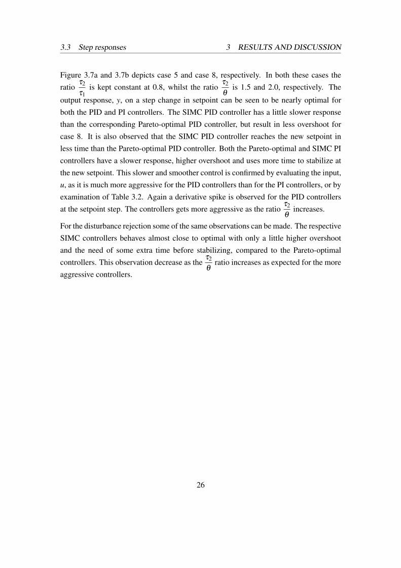
Figure 3.7a and 3.7b depicts case 5 and case 8, respectively. In both these cases theratio
τ2
τ1is kept constant at 0.8, whilst the ratio
τ2
θis 1.5 and 2.0, respectively. The
output response, y, on a step change in setpoint can be seen to be nearly optimal forboth the PID and PI controllers. The SIMC PID controller has a little slower responsethan the corresponding Pareto-optimal PID controller, but result in less overshoot forcase 8. It is also observed that the SIMC PID controller reaches the new setpoint inless time than the Pareto-optimal PID controller. Both the Pareto-optimal and SIMC PIcontrollers have a slower response, higher overshoot and uses more time to stabilize atthe new setpoint. This slower and smoother control is confirmed by evaluating the input,u, as it is much more aggressive for the PID controllers than for the PI controllers, or byexamination of Table 3.2. Again a derivative spike is observed for the PID controllersat the setpoint step. The controllers gets more aggressive as the ratio
τ2
θincreases.
For the disturbance rejection some of the same observations can be made. The respectiveSIMC controllers behaves almost close to optimal with only a little higher overshootand the need of some extra time before stabilizing, compared to the Pareto-optimalcontrollers. This observation decrease as the
τ2
θratio increases as expected for the more
aggressive controllers.
26
3.3 Step responses 3 RESULTS AND DISCUSSION
0 5 10 15 20 25 30 35 400
0.5
1
1.5
2
Output,
y
0 5 10 15 20 25 30 35 40
0
1
2
3
4
Input,
u
Time, t
Ms = 1.7 τ2
τ1= 0.8
τ2
θ= 1.5-- setpoint
PO (PID)
PO (PI)SIMC (PID)
SIMC(PI)
PO (PID)
PO (PI)
SIMC (PID)
SIMC(PI)
(a) Case 5, τ2θ= 1.5.
0 5 10 15 20 25 30 35 400
0.5
1
1.5
2
Output,
y
0 5 10 15 20 25 30 35 40
0
1
2
3
4
Input,
u
Time, t
Ms = 1.7 τ2
τ1= 0.8
τ2
θ= 2.0-- setpoint
PO (PID)
PO (PI)
SIMC (PID)
SIMC(PI)
PO (PID)
PO (PI)
SIMC (PID)
SIMC(PI)
(b) Case 8, τ2θ= 2.0.
Figure 3.7: Step responses for Pareto-optimal PID and PI, and SIMC PID and PI for secondorder plus time dealy processes on the form gp =
1(τ1s+1)(τ2s+1) ·exp(−θs). Ms = 1.7
and τ2τ1= 0.8.
27

3.3 Step responses 3 RESULTS AND DISCUSSION
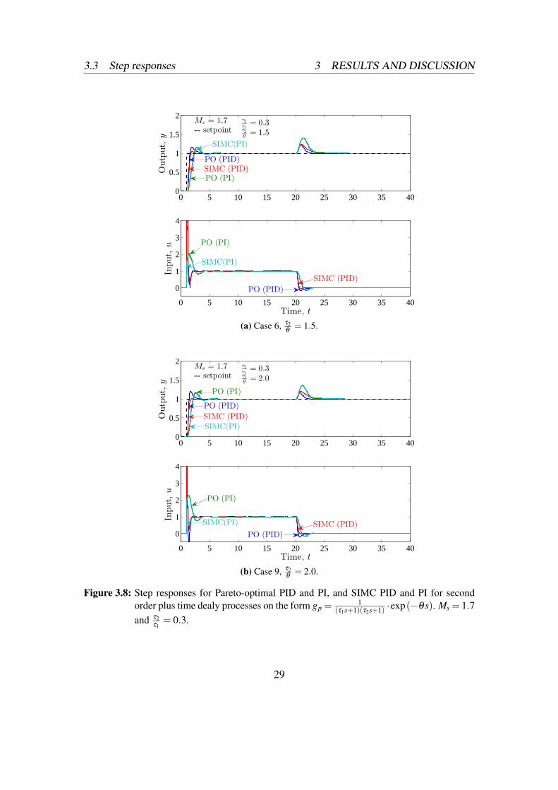
Figure 3.8a and 3.8b depicts case 6 and case 9, respectively. In both these cases the ratioτ2
τ1is kept constant at 0.3, whilst the ratio
τ2
θis 1.5 and 2.0, respectively. The output
performance, y, on a step change in setpoint can be seen to be nearly optimal for boththe PID and PI controllers. The SIMC PID controller has a less aggressive response thanthe corresponding Pareto-optimal PID controller, and thus result in less overshoot forboth cases. It is also observed that the SIMC PID controller reaches the new setpoint inless time than the Pareto-optimal PID controller. Both the Pareto-optimal and SIMC PIcontrollers have a slower response, higher overshoot and uses more time to stabilize atthe new setpoint. This slower, smoother control is confirmed by evaluating the input, u,as it is much more aggressive for the PID controllers than for the PI controllers. Again aderivative spike is observed for the PID controllers at the setpoint step. The controllersgets more aggressive as the ratio
τ2
θincreases.
For the disturbance rejection some of the same observations can be made. The respectiveSIMC controllers behaves almost close to optimal with only a little higher overshootand the need of some extra time before stabilizing, compared to the Pareto-optimalcontrollers. This observation decrease as the
τ2
θratio increases as expected for the more
aggressive controllers.
28
3.3 Step responses 3 RESULTS AND DISCUSSION
0 5 10 15 20 25 30 35 400
0.5
1
1.5
2
Output,y
0 5 10 15 20 25 30 35 40
0
1
2
3
4
Input,u
Time, t
Ms = 1.7 τ2
τ1= 0.3
τ2
θ= 1.5-- setpoint
PO (PID)
PO (PI)SIMC (PID)
SIMC(PI)
SIMC (PID)
PO (PI)
SIMC(PI)
PO (PID)
(a) Case 6, τ2θ= 1.5.
0 5 10 15 20 25 30 35 400
0.5
1
1.5
2
Output,y
0 5 10 15 20 25 30 35 40
0
1
2
3
4
Input,u
Time, t
Ms = 1.7 τ2
τ1= 0.3
τ2
θ= 2.0-- setpoint
PO (PID)
SIMC (PID)
PO (PID)
SIMC (PID)
PO (PI)
SIMC(PI)
PO (PI)
SIMC(PI)
(b) Case 9, τ2θ= 2.0.
Figure 3.8: Step responses for Pareto-optimal PID and PI, and SIMC PID and PI for secondorder plus time dealy processes on the form gp =
1(τ1s+1)(τ2s+1) ·exp(−θs). Ms = 1.7
and τ2τ1= 0.3.
29
3.4 Challenges and future work 3 RESULTS AND DISCUSSION
3.3.3 Summary step resonses
As depicted in Figures 3.6, 3.7 and 3.8 the SIMC tuning rules result in controllers witha good trade-off between setpoint performance and disturbance rejection, if tuningscorresponding to Ms = 1.7 is used. As can be seen from both the figures and the values inTable 3.2 the Pareto-optimal controllers behave more aggressive than the correspondingSIMC controllers. This result in enhanced disturbance rejection, for five out of six cases,while the performance of setpoint response is reduced.
The difference between the SIMC PID and PI controllers are seen to decrease as theratio
τ2
τ1decreases. As τ2 tends to zero, the PID and PI controllers should be the same.
Hence, this observation fits well with theory.
3.4 Challenges and future work
Throughout the work with this project the major challenge has been to obtain solutionsfrom the numeric solver in MATLAB. The problem at hand, is a minimization problemto a convex function and to find the right solution has not been easy. Many more caseshave been attempted, without been able to make them converge.
The cases tested in this project cannot be used as a satisfactory basis for any conclusionsregarding the SIMC tuning rules, but they can be used as a starting point. So far theSIMC tuning rules seems to perform close to optimal, and give good trade-off betweenperformance and robustness. For future work the solution algorithm may have to beimproved. In addition to be able to solve for Ms < 1.25 a broader specter of processescan be examined and more accurate conclusions can be drawn. Pareto-optimal tuningsfor a FOPTD process on the form: gp =
1s+1 ·e(−θs), should also be calculated to show
how much there is to profit from implementing a PID instead of a PI controller in thelimit as τ2 tend to zero.
30
4 CONCLUSIONS
4 Conclusions
The rather small selection of cases tested in the project does not give a solid foundationto build any conclusions on, however it can be used as a starting point. The performedcalculations and simulations show that the SIMC PID tuning rules give close to optimalperformance when Ms is used as a measure of robustness and a weighted function of theabsolute integral error is used as a measure for performance. The investigations showthat the recommended choice of not to implement a PID controller for time delay domi-nated process will be dependent on the process. For the three cases tested in this projectthe SIMC PI controller underperformed, on average, approximately 35 %. The perfor-mance reward by implementing a PID controller for these processes must be comparedwith the extra price and complexity a PID controller introduces. For the lag dominatedcases tested in this project the PID controller is shown to significantly overperform thePI controller, and thus the reward of implementing a PID controller is much greater thanfor the time delay dominated processes.
The recommended choice of the SIMC tuning parameter, τc = θ is shown to hold forprocesses with a
τ2
τ1ratio greater than 0.5. As the ratio decreases the corresponding Ms
values decreases, and the controller get more and more robust. As the trade-off betweenrobustness and performance always prevails, the controller performance is decreased. Ifthe τc value is decreased, the controller will lose some robustness, but gain performance.A τc = 0.5θ , or lower, is thus recommended to increase the performance.
Compared to the Pareto-optimal tunings, the SIMC tuning rules result in less aggres-sive controllers. These controllers have better setpoint performance, and slightly poorerdisturbance rejection.
31
REFERENCES REFERENCES
References
[1] S. Skogestad, “Simple analytic rules for model reduction and PID controller tun-ing,” J.Process Control, vol. 13, no. 4, pp. 291–309, 2003.
[2] S. Skogestad, “Probably the best simple PID tuning rules in the world,” 2001.
[3] C. Grimholdt and S. Skogestad, “Optimal PI-Control and Verification of the SIMCTuning Rule,” 2012.
[4] S. Skogestad and I. Postlethwaite, Multivariable Feedback Control Analysis andDesign. Chichester: John Wiley & Sons, 2012.
32
A MATLAB SCRIPTS
A MATLAB Scripts
In the following sections the different MATLAB scripts, used in this project, are pre-sented. They are presented in the order which they need to be executed, that is:
1. Pareto optimal PID tunings (mainOptimalTuningPID.m).
2. Pareto optimal PI tunings (mainOptimalTuningPI.m).
3. Pareto optimal vs. SIMC tunings (mainPoVsSimcPlot.m).
4. Step response (mainStepResponsePlotPo.m).
5. Parallel tunings (tuningParmParallel.m).
A.1 Obtain pareto optimal tunings
A.1.1 Optimal PID tunings, main file
1 % Script for generating the PO−PID curve for a given process gp
2 % The controller used is an ideal PID controller
3 % Written by: Martin S. Foss, fall 2012
4
5 %clc
6 clear all
7
8 global gp msEq iaeWeights manWeights iaeTuning
9
10 %Adding "sharedFiles" to MatLab search directory
11 curDir = pwd;
12 mainDir = fileparts(curDir);
13 sharedDir = fullfile(mainDir,'sharedFiles');
14 addpath(sharedDir);
15
16 %%
17 tic
18 modelId = 9;
A-1
A.1 Obtain pareto optimal tunings A MATLAB SCRIPTS
19 gp = model(modelId); %getting the model
20
21 %% Finding the iaeWeights
22 fprintf('Finding Optimal IAE Weights \n')
23 fprintf('Case: %g\n',modelId)
24 fprintf('***************************\n')
25 fprintf('\n')
26 fprintf('costFun(iae) \t minTuning \t\t Ms \t exitFlag \n')
27 fprintf('−−−−−−−−−−−−−−−−−−−−−−−−−−−−−−−−−−−−−−−−−−−−−−−−−\n')28
29 msEq = 1.59; %Ms for the iaeWeights
30 opt = optimset('algorithm','active−set','Display','off','TolCon',1e−4);31 %'active−set', 'trust−region−reflective', 'interior−point',32 %'interior−point−convex', 'levenberg−marquardt',33 %'trust−region−dogleg', 'lm−line−search', or 'sqp'.
34
35 %Initial solution guesses
36 X0 = [0.9 0.5 0.4 %case 1
37 1.0 0.6 0.6 %case 2
38 0.8 0.7 0.3 %case 3
39 2.2 1.5 0.8 %case 4
40 1.7 0.9 0.8 %case 5
41 3.2 2.4 0.8 %case 6
42 2.9 1.9 1.0 %case 7
43 2.2 1.2 1.0 %case 8
44 4.2 3.2 1.0]; %case 9
45 x0 = X0(modelId,:)';
46
47 iaeWeights = [1; 1]; %cost function weigths
48 manWeights = [1 0];
49
50 [minTuningSp,iaeSp,exitFlagSp] = fmincon(@costFun,x0,[],[],[],[],...
51 [0;0;0],[],@conFun,opt);
52
53 fprintf('%0.2f \t \t %.2f %.2f %.2f \t %.2f\t %i \t \n',iaeSp,...
54 minTuningSp, msEq, exitFlagSp)
55
56 %%
57 %Initial solution guesses
A-2
A.1 Obtain pareto optimal tunings A MATLAB SCRIPTS
58 X0 = [0.9 0.7 0.5 %case 1
59 1.0 0.6 0.6 %case 2
60 0.8 0.7 0.35 %case 3
61 2.2 2.3 0.8 %case 4
62 1.7 1.3 0.8 %case 5
63 3.3 5.0 0.8 %case 6
64 3.0 3.4 1.0 %case 7
65 2.2 1.8 1.0 %case 8
66 4.5 7.6 1.0]; %case 9
67 x0 = X0(modelId,:)';
68
69 manWeights = [0 1];
70
71 [minTuningD,iaeD,exitFlagD] = fmincon(@costFun,x0,[],[],[],[],....
72 [0;0;0],[],@conFun,opt);
73
74 fprintf('%0.2f \t \t %.2f %.2f %.2f \t %.2f\t %i \t \n',iaeD,...
75 minTuningD, msEq, exitFlagD)
76 fprintf('\n');
77 fprintf('\n');
78 fprintf('\n');
79 fprintf('\n');
80
81 iaeWeights = [iaeSp; iaeD];
82
83 %% Generating curve
84 i = 1; %iteration counter for command window printout
85 minTuning = []; %matrices for storing results
86 costTuning = [];
87 iaeOptTun = [];
88
89 msSpace = 1.25:0.05:3; %Ms search range
90
91 %Initial solution guesses
92 X0 = [0.7 0.5 0.4 %case 1
93 0.8 0.6 0.5 %case 2
94 0.4 0.4 0.3 %case 3
95 1.1 1.1 0.4 %case 4
96 0.9 0.7 0.5 %case 5
A-3

A.1 Obtain pareto optimal tunings A MATLAB SCRIPTS
97 1.6 1.9 0.4 %case 6
98 1.5 1.4 0.5 %case 7
99 1.1 0.9 0.6 %case 8
100 2.0 3.0 0.6]; %case 9
101 x0 = X0(modelId,:)';
102
103 manWeights = [.5, .5];
104
105 fprintf('Generating the PO Curve\n')
106 fprintf('***********************\n')
107 fprintf('\n')
108 fprintf('Number of iterations: %i \n', length(msSpace))
109 fprintf('\n')
110 fprintf('costFun(%.1f, %.1f) \t minTuning \t \t Ms ',manWeights)
111 fprintf('\t exitFlag \t iterations left \n')
112 fprintf('−−−−−−−−−−−−−−−−−−−−−−−−−−−−−−−−−−−−−−−−−−−−−−−−−−−−−−−−−−−−')113 fprintf('−−−−−−−−−−−−−−−−−−−−\n')114
115 opt = optimset('algorithm','active−set','Display','off','TolCon',1e−4);116 %'active−set', 'trust−region−reflective', 'interior−point',117 %'interior−point−convex', 'levenberg−marquardt',118 %'trust−region−dogleg', 'lm−line−search', or 'sqp'.
119
120 %Optimizing
121 for msEq = msSpace;
122
123 [minTuningTemp, iaeTuningTemp, exitFlagTuningTemp] = ...
124 fmincon(@costFun,x0,[],[],[],[],[0;0;0],[],@conFun,opt);
125
126 minTuning(:,i) = minTuningTemp; %storing resutlts
127 costTuning(i) = iaeTuningTemp;
128 exitFlagTuning(i) = exitFlagTuningTemp;
129 iaeOptTun(i,:) = iaeTuning;
130
131 if modelId == 2 && i == 1 || modelId == 3 && i == 1 ||...
132 modelId == 5 && i == 1
133 x0 = 1.1*minTuningTemp;
134 elseif modelId == 6 && i == 7 || modelId == 9 && i == 32
135 x0 = 0.9*minTuningTemp;
A-4
A.1 Obtain pareto optimal tunings A MATLAB SCRIPTS
136 elseif modelId == 9 && i == 17
137 x0 = 0.9*minTuningTemp;
138 elseif modelId == 9 && i == 16 || modelId == 9 && i >= 34
139 x0 = 0.91*minTuningTemp;
140 else
141 x0 = minTuningTemp;
142 end
143
144 fprintf('%0.2f \t \t \t %.2f %.2f %.2f \t %.2f\t %i \t \t\t %i \n',...
145 iaeTuningTemp, minTuningTemp, msEq, exitFlagTuningTemp,...
146 length(msSpace)−i)147
148 i = i + 1; %updating iteration counter
149 end
150
151 fprintf('\n')
152 fprintf('Calculation Finished!\n')
153 fprintf('=====================\n')
154 toc
155
156 %% Ploting the results
157 %Cost function, J vs. Ms
158 figure(modelId)
159 clf
160 h(1) = plot(msSpace,costTuning);
161 axis([1.2 3 0.8 1.3])
162 xlabel('Robustness, $M_s$', 'interpreter','latex','FontSize',14)
163 ylabel('Performance, $J$', 'interpreter','latex','FontSize',14)
164 titleName = {'Case 1','Case 2','Case 3','Case 4','Case 5',...
165 'Case 6','Case 7','Case 8','Case 9'};
166
167 title(titleName{modelId},'interpreter','latex','FontSize',14)
168
169 %% Storing results
170 modelName = {'case1','case2','case3','case4','case5','case6',...
171 'case7','case8','case9'};
172
173 res.case = num2str(modelName{modelId});
174
A-5
A.1 Obtain pareto optimal tunings A MATLAB SCRIPTS
175 res.POpid.minSp.tuning = minTuningSp;
176 res.POpid.minSp.iae = iaeSp;
177 res.POpid.minSp.exitFlag = exitFlagSp;
178
179 res.POpid.minD.tuning = minTuningD;
180 res.POpid.minD.iae = iaeD;
181 res.POpid.minD.exitFlag = exitFlagD;
182
183 res.POpid.minTuning.ms = msSpace;
184 res.POpid.minTuning.tuning = minTuning;
185 res.POpid.minTuning.costFun = costTuning;
186 res.POpid.minTuning.exitFlag = exitFlagTuning;
187 res.POpid.minTuning.iae = iaeOptTun;
188
189 % pause
190 % saving struct
191 save([mainDir,'\dataFiles\','resPOpid_',...
192 num2str(modelName{modelId}),'.mat'],'res') %saving "globaly"
193 save(['poPIDresults\','resPOpid_',...
194 num2str(modelName{modelId}),'.mat'],'res') %saving "localy"
195
196 % saving figures
197 saveas(h(1),['figures\','POpidCurve_',num2str(modelName{modelId}),'.fig'])
198
199 restoredefaultpath
A.1.2 Optimal PI tunings, main file
1 % Script for generating the PO−PI curve for a given process gp
2 % The controller used is an ideal PI controller
3 % Written by: Martin S. Foss, fall 2012
4
5 %clc
6 clear all
7
8 global gp msEq iaeWeights manWeights iaeTuning
9
10 %Adding "sharedFiles" to MatLab search directory
A-6
A.1 Obtain pareto optimal tunings A MATLAB SCRIPTS
11 curDir = pwd;
12 mainDir = fileparts(curDir);
13 sharedDir = fullfile(mainDir,'sharedFiles');
14 addpath(sharedDir);
15
16 %%
17 tic
18 modelId = 9;
19 modelName = {'case1','case2','case3','case4','case5','case6',...
20 'case7','case8','case9','case10'};
21 gp = model(modelId); % getting the model
22
23 %% Finding the iaeWeights for the PI−controller24 fprintf('Finding Optimal IAE Weights (PI−controller) \n')
25 fprintf('Case: %g\n',modelId)
26 fprintf('***************************\n')
27 fprintf('\n')
28 fprintf('costFun(iae) \t minTuning \t\t Ms \t exitFlag \n')
29 fprintf('−−−−−−−−−−−−−−−−−−−−−−−−−−−−−−−−−−−−−−−−−−−−−−−−−\n')30
31 msEq = 1.59; %Ms for the iaeWeights
32 opt = optimset('algorithm','active−set','Display','off','TolCon',1e−4);33 %'active−set', 'trust−region−reflective', 'interior−point',34 %'interior−point−convex', 'levenberg−marquardt',35 %'trust−region−dogleg', 'lm−line−search', or 'sqp'.
36
37 %Initial solution guesses
38 X0 = [0.5 0.4 0 %case 1
39 0.5 0.3 0 %case 2
40 0.5 0.4 0 %case 3
41 1.1 0.7 0 %case 4
42 0.8 0.5 0 %case 5
43 1.5 1.2 0 %case 6
44 1.3 0.9 0 %case 7
45 1.0 0.6 0 %case 8
46 1.9 1.4 0]; %case 9
47 x0 = X0(modelId,:)';
48
49 iaeWeights = [1; 1]; %cost function weigths
A-7
A.1 Obtain pareto optimal tunings A MATLAB SCRIPTS
50 manWeights = [1 0];
51
52 Aeq = [0 0 1]; %constraints
53 Beq = 0;
54
55 [minTuningSp,iaeSp,exitFlagSp] = fmincon(@costFun,x0,[],[],Aeq,Beq,...
56 [0;0;0],[],@conFun,opt);
57
58 fprintf('%0.2f \t \t %.2f %.2f %.2f \t %.2f\t %i \t \n',iaeSp,...
59 minTuningSp, msEq, exitFlagSp)
60
61 %%
62 %Initial solution guesses
63 X0 = [0.5 0.4 0 %case 1
64 0.5 0.3 0 %case 2
65 0.5 0.4 0 %case 3
66 0.9 0.8 0 %case 4
67 0.7 0.5 0 %case 5
68 1.3 1.3 0 %case 6
69 1.1 0.9 0 %case 7
70 0.9 0.6 0 %case 8
71 1.5 1.6 0]; %case 9
72 x0 = X0(modelId,:)';
73
74 manWeights = [0 1];
75
76 [minTuningD,iaeD,exitFlagD] = fmincon(@costFun,x0,[],[],Aeq,Beq,...
77 [0;0;0],[],@conFun,opt);
78
79 fprintf('%0.2f \t \t %.2f %.2f %.2f \t %.2f\t %i \t \n',iaeD,...
80 minTuningD, msEq, exitFlagD)
81 fprintf('\n');
82 fprintf('\n');
83 fprintf('\n');
84 fprintf('\n');
85
86 %% Generating curve
87 try
88 load(fullfile(mainDir,'dataFiles',['resPOpid_',...
A-8

A.1 Obtain pareto optimal tunings A MATLAB SCRIPTS
89 num2str(modelName{modelId}),'.mat']))
90 catch me
91 ME = MException(me.identifier,...
92 'could not open file, check corrrect modelId and data folder!');
93 throw(ME)
94 end
95 minSp = res.POpid.minSp.iae;
96 minD = res.POpid.minD.iae;
97 iaeWeights = [minSp; minD];
98
99 i = 1; %iteration counter for command window printout
100 minTuning = []; %matrices for storing results
101 costTuning = [];
102 iaeOptTun = [];
103
104 msSpace = 1.25:0.05:3; %the Ms search range
105
106 %Initial solution guesses
107 X0 = [0.2 0.2 0 %case 1
108 0.3 0.2 0 %case 2
109 0.2 0.2 0 %case 3
110 0.4 0.4 0 %case 4
111 0.5 0.4 0 %case 5
112 0.6 0.6 0 %case 6
113 0.5 0.4 0 %case 7
114 0.4 0.3 0 %case 8
115 1.2 1.1 0]; %case 9
116 x0 = X0(modelId,:)';
117
118 manWeights = [.5, .5];
119
120 fprintf('Generating the PO Curve\n')
121 fprintf('***********************\n')
122 fprintf('\n')
123 fprintf('Number of iterations: %i \n', length(msSpace))
124 fprintf('\n')
125 fprintf('costFun(%.1f, %.1f) \t minTuning \t \t Ms',manWeights)
126 fprintf(' \t exitFlag \t iterations left \n')
127 fprintf('−−−−−−−−−−−−−−−−−−−−−−−−−−−−−−−−−−−−−−−−−−−−−−−−−−−−−−−−−−−−')
A-9
A.1 Obtain pareto optimal tunings A MATLAB SCRIPTS
128 fprintf('−−−−−−−−−−−−−−−−−−−−\n')129
130 opt = optimset('algorithm','active−set','Display','off','TolCon',1e−4);131 %'active−set', 'trust−region−reflective', 'interior−point',132 %'interior−point−convex', 'levenberg−marquardt',133 %'trust−region−dogleg', 'lm−line−search', or 'sqp'.
134
135 %Optimizing
136 for msEq = msSpace;
137
138 [minTuningTemp, iaeTuningTemp, exitFlagTuningTemp] = ...
139 fmincon(@costFun,x0,[],[],Aeq,Beq,[0;0;0],[],@conFun,opt);
140
141 minTuning(:,i) = minTuningTemp; %storing resutlts
142 costTuning(i) = iaeTuningTemp;
143 exitFlagTuning(i) = exitFlagTuningTemp;
144 iaeOptTun(i,:) = iaeTuning;
145
146 if modelId == 1 && i == 22 || modelId == 1 && i == 32 || ...
147 modelId == 3 && i == 22 || modelId == 9 && i == 29 || ...
148 modelId == 9 && i >= 32
149 x0 = 0.9*minTuningTemp;
150 elseif modelId == 5 && i == 1 || modelId == 5 && i == 2
151 x0 = 1.2*minTuningTemp;
152 else
153 x0 = minTuningTemp;
154 end
155
156 fprintf('%0.2f \t \t \t %.2f %.2f %.2f \t %.2f\t %i \t \t\t %i \n',...
157 iaeTuningTemp, minTuningTemp, msEq, exitFlagTuningTemp,...
158 length(msSpace)−i)159
160 i = i + 1; %updating iteration counter
161 end
162
163 fprintf('\n')
164 fprintf('Calculation Finished!\n')
165 fprintf('=====================\n')
166 toc
A-10
A.1 Obtain pareto optimal tunings A MATLAB SCRIPTS
167
168 %% Plotting the results
169 % Cost function, J, vs. Ms
170 figure(modelId)
171 clf
172 h(1) = plot(msSpace,costTuning);
173 xlabel('Robustness, $M_s$', 'interpreter','latex','FontSize',14)
174 ylabel('Performance, $J$', 'interpreter','latex','FontSize',14)
175 titleName = {'Case 1','Case 2','Case 3','Case 4','Case 5',...
176 'Case 6','Case 7','Case 8','Case 9',};
177
178 title(titleName{modelId},'interpreter','latex','FontSize',14)
179
180 %% Storing results (in the same struct as the PO (PID) tunings)
181 res.POpi.minSp.tuning = minTuningSp;
182 res.POpi.minSp.iae = iaeSp;
183 res.POpi.minSp.exitFlag = exitFlagSp;
184
185 res.POpi.minD.tuning = minTuningD;
186 res.POpi.minD.iae = iaeD;
187 res.POpi.minD.exitFlag = exitFlagD;
188
189 res.POpi.minTuning.ms = msSpace;
190 res.POpi.minTuning.tuning = minTuning;
191 res.POpi.minTuning.costFun = costTuning;
192 res.POpi.minTuning.exitFlag = exitFlagTuning;
193 res.POpi.minTuning.iae = iaeOptTun;
194
195 pause
196 %saving struct
197 save([mainDir,'\dataFiles\','resPO_',...
198 num2str(modelName{modelId}),'.mat'],'res')
199 save(['poPIresults\','resPO_',...
200 num2str(modelName{modelId}),'.mat'],'res')
201
202 %saving figures
203 saveas(h(1),['figures\','POpiCurve_',num2str(modelName{modelId}),'.fig'])
204
205 restoredefaultpath
A-11
A.2 Obtain PO vs. SIMC tuning plots A MATLAB SCRIPTS
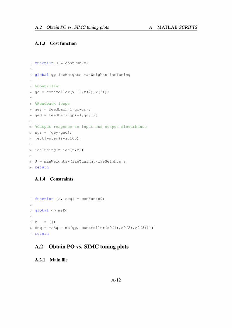
A.1.3 Cost function
1 function J = costFun(x)
2
3 global gp iaeWeights manWeights iaeTuning
4
5 %Controller
6 gc = controller(x(1),x(2),x(3));
7
8 %Feedback loops
9 gey = feedback(1,gc*gp);
10 ged = feedback(gp*−1,gc,1);11
12 %Output response to input and output disturbance
13 sys = [gey;ged];
14 [e,t]=step(sys,100);
15
16 iaeTuning = iae(t,e);
17
18 J = manWeights*(iaeTuning./iaeWeights);
19 return
A.1.4 Constraints
1 function [c, ceq] = conFun(x0)
2
3 global gp msEq
4
5 c = [];
6 ceq = msEq − ms(gp, controller(x0(1),x0(2),x0(3)));
7 return
A.2 Obtain PO vs. SIMC tuning plots
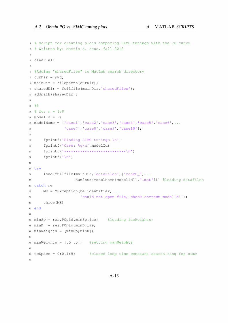
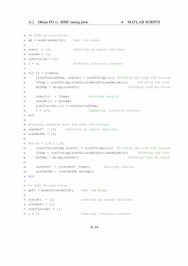
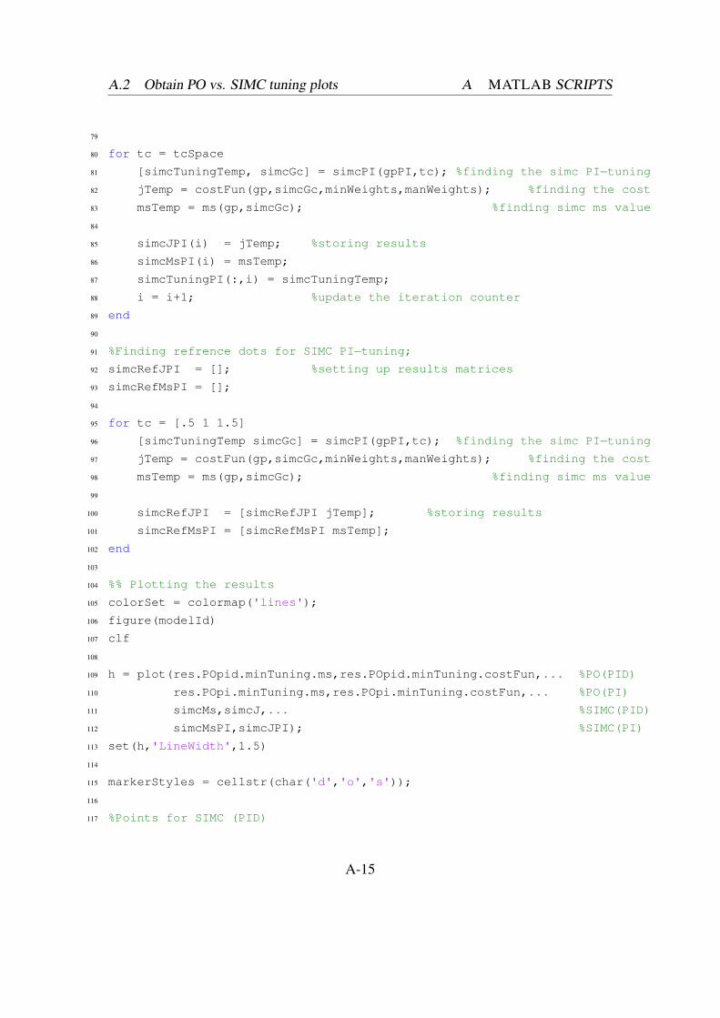
A.2.1 Main file
A-12
A.2 Obtain PO vs. SIMC tuning plots A MATLAB SCRIPTS
1 % Script for creating plots comparing SIMC tunings with the PO curve
2 % Written by: Martin S. Foss, fall 2012
3
4 clear all
5
6 %Adding "sharedFiles" to MatLab search directory
7 curDir = pwd;
8 mainDir = fileparts(curDir);
9 sharedDir = fullfile(mainDir,'sharedFiles');
10 addpath(sharedDir);
11
12 %%
13 % for m = 1:8
14 modelId = 9;
15 modelName = {'case1','case2','case3','case4','case5','case6',...
16 'case7','case8','case9','case10'};
17
18 fprintf('Finding SIMC tunings \n')
19 fprintf('Case: %g\n',modelId)
20 fprintf('***************************\n')
21 fprintf('\n')
22
23 try
24 load(fullfile(mainDir,'dataFiles',['resPO_',...
25 num2str(modelName{modelId}),'.mat'])) %loading datafiles
26 catch me
27 ME = MException(me.identifier,...
28 'could not open file, check correct modelId!');
29 throw(ME)
30 end
31
32 minSp = res.POpid.minSp.iae; %loading iaeWeights;
33 minD = res.POpid.minD.iae;
34 minWeights = [minSp;minD];
35
36 manWeights = [.5 .5]; %setting manWeights
37
38 tcSpace = 0:0.1:5; %closed loop time constant search rang for simc
39
A-13
A.2 Obtain PO vs. SIMC tuning plots A MATLAB SCRIPTS
40 %% SIMC PI−controller41 gp = model(modelId); %get the model
42
43 simcJ = []; %setting up result matrices
44 simcMs = [];
45 simcTuning = [];
46 i = 1; %setting iteration counter
47
48 for tc = tcSpace
49 [simcTuningTemp, simcGc] = simcPID(gp,tc); %finding the simc PID tuning
50 jTemp = costFun(gp,simcGc,minWeights,manWeights); %finding the cost
51 msTemp = ms(gp,simcGc); %finding simc ms value
52
53 simcJ(i) = jTemp; %storing results
54 simcMs(i) = msTemp;
55 simcTuning(:,i) = simcTuningTemp;
56 i = i+1; %updating iteration counter
57 end
58
59 %Finding refrence dots for SIMC PID−tuning;60 simcRefJ = []; %setting up result matrices
61 simcRefMs = [];
62
63 for tc = [.5 1 1.5]
64 [simcTuningTemp simcGc] = simcPID(gp,tc); %finding the simc PID tuning
65 jTemp = costFun(gp,simcGc,minWeights,manWeights); %finding the cost
66 msTemp = ms(gp,simcGc); %finding simc ms value
67
68 simcRefJ = [simcRefJ jTemp]; %storing results
69 simcRefMs = [simcRefMs msTemp];
70 end
71
72 %% SIMC PI−controller73 gpPI = modelPI(modelId); %get the model
74
75 simcJPI = []; %setting up result matrices
76 simcMsPI = [];
77 simcTuningPI = [];
78 i = 1; %setting iteration counter
A-14
A.2 Obtain PO vs. SIMC tuning plots A MATLAB SCRIPTS
79
80 for tc = tcSpace
81 [simcTuningTemp, simcGc] = simcPI(gpPI,tc); %finding the simc PI−tuning82 jTemp = costFun(gp,simcGc,minWeights,manWeights); %finding the cost
83 msTemp = ms(gp,simcGc); %finding simc ms value
84
85 simcJPI(i) = jTemp; %storing results
86 simcMsPI(i) = msTemp;
87 simcTuningPI(:,i) = simcTuningTemp;
88 i = i+1; %update the iteration counter
89 end
90
91 %Finding refrence dots for SIMC PI−tuning;92 simcRefJPI = []; %setting up results matrices
93 simcRefMsPI = [];
94
95 for tc = [.5 1 1.5]
96 [simcTuningTemp simcGc] = simcPI(gpPI,tc); %finding the simc PI−tuning97 jTemp = costFun(gp,simcGc,minWeights,manWeights); %finding the cost
98 msTemp = ms(gp,simcGc); %finding simc ms value
99
100 simcRefJPI = [simcRefJPI jTemp]; %storing results
101 simcRefMsPI = [simcRefMsPI msTemp];
102 end
103
104 %% Plotting the results
105 colorSet = colormap('lines');
106 figure(modelId)
107 clf
108
109 h = plot(res.POpid.minTuning.ms,res.POpid.minTuning.costFun,... %PO(PID)
110 res.POpi.minTuning.ms,res.POpi.minTuning.costFun,... %PO(PI)
111 simcMs,simcJ,... %SIMC(PID)
112 simcMsPI,simcJPI); %SIMC(PI)
113 set(h,'LineWidth',1.5)
114
115 markerStyles = cellstr(char('d','o','s'));
116
117 %Points for SIMC (PID)
A-15
A.2 Obtain PO vs. SIMC tuning plots A MATLAB SCRIPTS
118 hold on
119 for i = 1:length(simcRefMs)
120 h(i) = plot(simcRefMs(i),simcRefJ(i));
121 set(h(i),'color',colorSet(3,:),'LineWidth',1.5,'Marker',...
122 markerStyles{i},'MarkerSize',10);
123 end
124
125 axis([1 3 0.75 8]);
126
127 %Points for SIMC (PI)
128 for i = 1:length(simcRefMsPI)
129 h(i) = plot(simcRefMsPI(i),simcRefJPI(i));
130 set(h(i),'color',colorSet(4,:),'linewidth',1.5,'Marker',...
131 markerStyles{i},'MarkerSize',10);
132 end
133
134 %% Printing info
135 tau2tau1Info = {'$\frac{\tau_2}{\tau_1}=0.5$',...
136 '$\frac{\tau_2}{\tau_1}=0.8$',...
137 '$\frac{\tau_2}{\tau_1}=0.3$',...
138 '$\frac{\tau_2}{\tau_1}=0.5$',...
139 '$\frac{\tau_2}{\tau_1}=0.8$',...
140 '$\frac{\tau_2}{\tau_1}=0.3$',...
141 '$\frac{\tau_2}{\tau_1}=0.5$',...
142 '$\frac{\tau_2}{\tau_1}=0.8$',...
143 '$\frac{\tau_2}{\tau_1}=0.3$'};
144 tau2thetaInfo = {'$\frac{\tau_2}{\theta}=0.5$',...
145 '$\frac{\tau_2}{\theta}=0.8$',...
146 '$\frac{\tau_2}{\theta}=0.3$',...
147 '$\frac{\tau_2}{\theta}=1.5$',...
148 '$\frac{\tau_2}{\theta}=1.5$',...
149 '$\frac{\tau_2}{\theta}=1.5$',...
150 '$\frac{\tau_2}{\theta}=2.0$',...
151 '$\frac{\tau_2}{\theta}=2.0$',...
152 '$\frac{\tau_2}{\theta}=2.0$'};
153 curveInfo = {'PO (PID)','PO (PI)','SIMC (PID)','SIMC(PI)'};
154 pointInfo = {'$\tau_c=0.5\theta$','$\tau_c=\theta$','$\tau_c=1.5\theta$'};
155
156 infoFontSize = 18;
A-16
A.2 Obtain PO vs. SIMC tuning plots A MATLAB SCRIPTS
157
158 xlab = xlabel('Robustness, $M_s$');
159 ylab = ylabel('Performance, $J(c)$');
160 set(xlab,'interpreter','latex','fontsize',infoFontSize)
161 set(ylab,'interpreter','latex','fontsize',infoFontSize)
162
163 set(gca,'fontsize',16,'FontName','Times New Roman')
164
165 %Model info
166 [figx figy] = dsxy2figxy(gca,2.4,5.5);
167 textBoxTau1Tau2Info = annotation('textbox',[figx figy .07 .03],...
168 'string',tau2tau1Info{modelId},'interpreter','latex',...
169 'fontsize',infoFontSize,'color',[0 0 0],'FitBoxToText','on',...
170 'LineStyle','none');
171
172 [figx figy] = dsxy2figxy(gca,2.4,5); % (gca,3,3)
173 textBoxTau2ThetaInfo = annotation('textbox',[figx figy .07 .03],...
174 'string',tau2thetaInfo{modelId},'interpreter','latex',...
175 'fontsize',infoFontSize,'color',[0 0 0],'FitBoxToText','on',...
176 'LineStyle','none');
177
178 %Markers for different tau_c
179 h = plot(2.4,4.5,'marker',markerStyles{1},'markerSize',10,...
180 'linewidth',1.5,'color',[0 0 0]);
181 [figx figy] = dsxy2figxy(gca,2.4,4.5);
182 point1 = annotation('textarrow',[figx+0.025 figx+0.015],[figy figy],...
183 'string',pointInfo{1},'interpreter','latex',...
184 'fontsize',infoFontSize,'headstyle','none');
185
186 h = plot(2.4,4,'marker',markerStyles{2},'markerSize',10,...
187 'linewidth',1.5,'color',[0 0 0]);
188 [figx figy] = dsxy2figxy(gca,2.4,4);
189 point2 = annotation('textarrow',[figx+0.025 figx+0.015],[figy figy],...
190 'string',pointInfo{2},'interpreter','latex',...
191 'fontsize',infoFontSize,'headstyle','none');
192
193 h = plot(2.4,3.5,'marker',markerStyles{3},'markerSize',10,...
194 'linewidth',1.5,'color',[0 0 0]);
195 [figx figy] = dsxy2figxy(gca,2.4,3.5);
A-17
A.2 Obtain PO vs. SIMC tuning plots A MATLAB SCRIPTS
196 point3 = annotation('textarrow',[figx+0.025 figx+0.015],[figy figy],...
197 'string',pointInfo{3},'interpreter','latex',...
198 'fontsize',infoFontSize,'headstyle','none');
199
200 %PO (PID)
201 if modelId == 8
202 x1 = find(res.POpid.minTuning.ms >= 1.4);
203 else
204 x1 = find(res.POpid.minTuning.ms >= 1.5);
205 end
206 [figx figy] = dsxy2figxy(gca,res.POpid.minTuning.ms(x1(1)),...
207 res.POpid.minTuning.costFun(x1(1)));
208 curve1 = annotation('textarrow',[figx−0.03 figx],[figy−0.005 figy],...
209 'string',curveInfo{1},'interpreter','latex',...
210 'fontsize',infoFontSize,'color',colorSet(1,:));
211
212 %PO (PI)
213 x2 = find(res.POpi.minTuning.ms >= 2.4);
214 [figx figy] = dsxy2figxy(gca,res.POpi.minTuning.ms(x2(1)),...
215 res.POpi.minTuning.costFun(x2(1)));
216 if modelId < 4
217 curve2 = annotation('textarrow',[figx+0.05 figx],[figy+0.05 figy],...
218 'string',curveInfo{2},'interpreter','latex',...
219 'fontsize',infoFontSize,'color',colorSet(2,:));
220 else
221 curve2 = annotation('textarrow',[figx+0.05 figx],[figy−0.05 figy],...
222 'string',curveInfo{2},'interpreter','latex',...
223 'fontsize',infoFontSize,'color',colorSet(2,:));
224 end
225
226 %SIMC (PID)
227 if modelId == 1 || modelId == 2 || modelId == 3
228 x3 = find(simcMs <= 1.20);
229 elseif modelId == 7
230 x3 = find(simcMs <= 1.3);
231 else
232 x3 = find(simcMs <= 1.4);
233 end
234 [figx figy] = dsxy2figxy(gca,simcMs(x3(1)),simcJ(x3(1)));
A-18
A.2 Obtain PO vs. SIMC tuning plots A MATLAB SCRIPTS
235 if modelId == 4
236 curve3 = annotation('textarrow',[figx+0.05 figx],[figy+0.01 figy],...
237 'string',curveInfo{3},'interpreter','latex',...
238 'fontsize',infoFontSize,'color',colorSet(3,:));
239 else
240 curve3 = annotation('textarrow',[figx+0.05 figx],[figy figy],...
241 'string',curveInfo{3},'interpreter','latex',...
242 'fontsize',infoFontSize,'color',colorSet(3,:));
243 end
244
245 %SIMC (PI)
246 if modelId == 5 || modelId == 7
247 x4 = find(simcMsPI <= 2.1);
248 else
249 x4 = find(simcMsPI <= 2);
250 end
251 [figx figy] = dsxy2figxy(gca,simcMsPI(x4(1)),simcJPI(x4(1)));
252 curve4 = annotation('textarrow',[figx+0.02 figx],[figy+0.03 figy],...
253 'string',curveInfo{4},'interpreter','latex',...
254 'fontsize',infoFontSize,'color',colorSet(4,:));
255
256 set(gca,'Layer','top','Box','on')
257 set(gcf,'paperpositionmode','auto')
258
259 %% Storing results and figures
260 res.simcPID.simcJ = simcJ;
261 res.simcPID.simcMs = simcMs;
262 res.simcPID.simcTuning = simcTuning;
263
264 res.simcPI.simcJ = simcJPI;
265 res.simcPI.simcMs = simcMsPI;
266 res.simcPI.simcTuning = simcTuningPI;
267
268 pause
269 save([mainDir,'\dataFiles\','resSimc_',...
270 num2str(modelName{modelId}),'.mat'],'res')
271 save(['simcResults\','resSimc_',num2str(modelName{modelId}),'.mat'],'res')
272
273 saveas(h,['SIMCfigures\','simcRes_',...
A-19
A.2 Obtain PO vs. SIMC tuning plots A MATLAB SCRIPTS
274 num2str(modelName{modelId}),'.eps'],'psc2')
275 saveas(h,['SIMCfigures\','simcRes_',num2str(modelName{modelId}),'.fig'])
276 % end
277
278 restoredefaultpath
A.2.2 Cost function
1 function J = costFun(gp,gc,iaeWeights,manWeights)
2
3 %Feedback loops
4 gey = feedback(1,gc*gp);
5 ged = feedback(gp*−1,gc,1);6
7 %Output response to input and output disturbance
8 sys = [gey;ged];
9 [e,t] = step(sys,100);
10
11 iaeTuning = iae(t,e);
12
13 J = manWeights*(iaeTuning./iaeWeights);
14 return
A.2.3 SIMC PI-tunings
1 % function for simc PI tuning
2 % input: 2nd order model + tuning parameter
3 % returns: simc tuning paramer for a PI controller on the form
4 % gc = K + I/s
5 % Written by: Martin S. Foss, fall 2012
6
7 function [tuning gc] = simcPI(gp,tc)
8
9 %Determining the model
10 t = gp.den{1}(1); %time constant
11 d = totaldelay(gp); %time delay
12 g = gp.num{1}(end); %gain
A-20
A.2 Obtain PO vs. SIMC tuning plots A MATLAB SCRIPTS
13 z = zero(gp); %zeros
14 p = pole(gp); %poles
15
16 if length(gp.den{1}) > 2
17 disp('model order to high')
18 return
19 elseif isempty(z) == 0
20 disp('model cannot contain zeros')
21 return
22 end
23
24 K = t/(g*(tc+d));
25 I = K/min(t,4*(tc+d));
26
27 tuning = [K I]';
28 [gcPID gc] = controller(K,I);
29 return
A.2.4 SIMC PID-tunings
1 % function for simc PID tuning
2 % input: 2nd order model + tuning parameter
3 % returns: simc tuning paramer for a PID controller on the form
4 % gc = K + I/s + D*s
5 % Written by: Martin S. Foss, fall 2012
6
7 function [tuning, gc] = simcPID(gp,tc)
8
9 %Determining the model
10 d = totaldelay(gp); %time delay
11 g = gp.num{1}(end); %gain
12 z = zero(gp); %zeros
13 p = pole(gp); %poles
14 t1 = abs(p(2)); %time constant 1 (largest)
15 t2 = abs(p(2)/p(1)); %time constant 2 (smallest)
16
17 if nargin == 1
18 tc = d;
A-21
A.2 Obtain PO vs. SIMC tuning plots A MATLAB SCRIPTS
19 end
20
21 if length(gp.den{1}) > 3
22 disp('model order to high')
23 return
24 elseif isempty(z) == 0
25 disp('model cannot contain zeros')
26 return
27 end
28
29 %SIMC−tuning (series)
30 Kc = 1/g*(t1/(tc+d));
31 taui = min(t1,4*(tc+d));
32 taud = t2;
33
34 %SIMC−tuning (parallel)
35 K_merk = Kc*(1+taud/taui);
36 I_merk = taui*(1+taud/taui);
37 D_merk = taud/(1+taud/taui);
38
39 %SIMC−tuning (given parameterization)
40 K = K_merk;
41 I = K_merk/I_merk;
42 D = K_merk*D_merk;
43
44 tuning = [K I D]';
45 gc = controller(K,I,D);
46 return
A-22
A.3 Obtain step responses A MATLAB SCRIPTS
A.3 Obtain step responses
A.3.1 Main file
1 % Script evaluating step response for PID controller using both PO and SIMC
2 % controller tunings
3 % Written by: Martin S. Foss, fall 2012
4
5 clear all
6 % close all
7 clc
8
9 %Adding "sharedFiles" to MatLab search directory
10 curDir = pwd;
11 mainDir = fileparts(curDir);
12 sharedDir = fullfile(mainDir,'sharedFiles');
13 addpath(sharedDir);
14
15 % for m = 1:8
16 modelId = 9; %m;
17 modelName = {'case1','case2','case3','case4','case5','case6',...
18 'case7','case8','case9','case10'};
19 msSet = 1.7; %define the Ms value
20
21 load(fullfile(mainDir,'dataFiles',['resSimc_',...
22 num2str(modelName{modelId}),'.mat'])) %loading datafiles
23
24 %Collecting PO and SIMC tunings
25 index = find(res.POpid.minTuning.ms == msSet);
26 tuning{1} = res.POpid.minTuning.tuning(:,index(1));
27
28 index2 = find(res.POpi.minTuning.ms == msSet);
29 tuning{2} = res.POpi.minTuning.tuning(:,index2(1));
30
31 index3 = find(res.simcPID.simcMs <= msSet);
32 tuning{3} = res.simcPID.simcTuning(:,index3(1));
33
34 index4 = find(res.simcPI.simcMs <= msSet);
A-23
A.3 Obtain step responses A MATLAB SCRIPTS
35 tuning{4} = res.simcPI.simcTuning(:,index4(1));
36
37 gp = model(modelId); %loading the model
38
39 %Extracting parameters from the model
40 p = pole(gp); %poles
41 t1 = abs(p(2)); %time constant 1 (largest)
42 t2 = abs(p(2)/p(1)); %time constant 2 (smallest) = taud
43
44 %% Plotting PO (PID) and SIMC (PID)
45 ysTime = 1; %define simaulation parameters
46 dTime = 20;
47 stopTime = 40;
48
49 figure(modelId)
50 clf
51 colorSet = colormap('lines');
52
53 Y = []; %setting up result matrices
54 U = [];
55 T = [];
56
57 for i = [1 3]
58 subplot(2,1,1)
59 gc = controller(tuning{i}(1),tuning{i}(2),tuning{i}(3),t2);
60 sim('simModel') %running Simulink
61
62 r = plot(t,y); %plotting output vs. time
63 set(r,'Color',colorSet(i,:),'LineWidth',1.5);
64 axis([0 stopTime 0 2])
65 hold on
66
67 subplot(2,1,2)
68 r = plot(t,u); %plotting input vs. time
69 set(r,'Color',colorSet(i,:),'LineWidth',1.5);
70 axis([0 40 −.5 4])
71 hold on
72
73 Y{i} = y; %storing results
A-24
A.3 Obtain step responses A MATLAB SCRIPTS
74 U{i} = u;
75 T{i} = t;
76 end
77
78 %% Plotting PO (PI) and SIMC (PI)
79 for k = [2 4]
80 subplot(2,1,1)
81 [a gc] = controller(tuning{k}(1),tuning{k}(2));
82 sim('simModel');
83 r = plot(t,y); %plotting output vs. time
84 set(r,'Color',colorSet(k,:),'LineWidth',1.5);
85
86 subplot(2,1,2)
87 r = plot(t,u); %plotting inputs vs. time
88 set(r,'Color',colorSet(k,:),'LineWidth',1.5);
89
90 Y{k} = y; %storing results
91 U{k} = u;
92 T{k} = t;
93 end
94
95 subplot(211)
96 r = plot(t,ys,'−−k','linewidth',1.5); %plotting setpoint
97 set(r,'Color',[0 0 0],'LineWidth',1.5,'LineStyle','−−');98
99 %% Printing info
100 caseInfo = {'$\frac{\tau_2}{\tau_1}=0.5$ $\frac{\tau_2}{\theta}=0.5$',...
101 '$\frac{\tau_2}{\tau_1}=0.8$ $\frac{\tau_2}{\theta}=0.8$',...
102 '$\frac{\tau_2}{\tau_1}=0.3$ $\frac{\tau_2}{\theta}=0.3$',...
103 '$\frac{\tau_2}{\tau_1}=0.5$ $\frac{\tau_2}{\theta}=1.5$',...
104 '$\frac{\tau_2}{\tau_1}=0.8$ $\frac{\tau_2}{\theta}=1.5$',...
105 '$\frac{\tau_2}{\tau_1}=0.3$ $\frac{\tau_2}{\theta}=1.5$',...
106 '$\frac{\tau_2}{\tau_1}=0.5$ $\frac{\tau_2}{\theta}=2.0$',...
107 '$\frac{\tau_2}{\tau_1}=0.8$ $\frac{\tau_2}{\theta}=2.0$',...
108 '$\frac{\tau_2}{\tau_1}=0.3$ $\frac{\tau_2}{\theta}=2.0$'};
109 curveInfo = {'PO (PID)','PO (PI)','SIMC (PID)','SIMC(PI)'};
110 msString={'$M_s$ $=$ $1.7$'};
111
112 stdFont = 16;
A-25
A.3 Obtain step responses A MATLAB SCRIPTS
113 infoFontSize = 18;
114
115 subplot(211)
116 ylab = ylabel('Output, $y$');
117 set(ylab,'interpreter','latex','fontsize',infoFontSize)
118 set(gca,'fontsize',stdFont,'FontName','Times New Roman')
119
120 subplot(212)
121 ylab = ylabel('Input, $u$');
122 xlab = xlabel('Time, $t$');
123 set(xlab,'interpreter','latex','fontsize',infoFontSize)
124 set(ylab,'interpreter','latex','fontsize',infoFontSize)
125 set(gca,'fontsize',stdFont,'FontName','Times New Roman')
126
127 subplot(211)
128 [figx figy] = dsxy2figxy(gca,1.9,1.8); % (gca,3,3)
129 textBoxMs = annotation('textbox',[figx figy .07 .03],'string',...
130 msString{1},'interpreter','latex','fontsize',stdFont,...
131 'color',[0 0 0],'FitBoxToText','on','LineStyle','none');
132
133 [figx figy] = dsxy2figxy(gca,10,1.75); % (gca,3,3)
134 textBoxCaseInfo = annotation('textbox',[figx figy .07 .03],'string',...
135 caseInfo{modelId},'interpreter','latex','fontsize',...
136 stdFont,'color',[0 0 0],'FitBoxToText','off',...
137 'LineStyle','none');
138
139 [figx figy] = dsxy2figxy(gca,1.9,1.55); % (gca,3,3)
140 textBoxSetPoint = annotation('textbox',[figx, figy, .07 .03],'string',...
141 '{\bf−}{\bf−} setpoint','interpreter','latex',...
142 'fontsize',stdFont,'color',[0 0 0],'FitBoxToText',...
143 'on','LineStyle','none');
144
145 %PO (PID)
146 y1 = find(Y{1}>=0.8);
147 [figx figy] = dsxy2figxy(gca,T{1}(y1(1)),Y{1}(y1(1)));
148 curve1 = annotation('textarrow',[figx+0.05 figx],[figy figy],...
149 'string',curveInfo{1},'interpreter','latex','fontsize',stdFont,...
150 'color',colorSet(1,:));
151
A-26
A.3 Obtain step responses A MATLAB SCRIPTS
152 %PO (PI)
153 y2 = find(Y{2}>=0.25);
154 [figx figy] = dsxy2figxy(gca,T{2}(y2(1)),Y{2}(y2(1)));
155 curve2 = annotation('textarrow',[figx+0.05 figx],[figy figy],...
156 'string',curveInfo{2},'interpreter','latex','fontsize',stdFont,...
157 'color',colorSet(2,:));
158
159 %SIMC (PID)
160 y3 = find(Y{3}>=0.5);
161 [figx figy] = dsxy2figxy(gca,T{3}(y3(1)),Y{3}(y3(1)));
162 curve3 = annotation('textarrow',[figx+0.05 figx],[figy figy],...
163 'string',curveInfo{3},'interpreter','latex','fontsize',stdFont,...
164 'color',colorSet(3,:));
165
166 %SIMC (PI)
167 [y4val y4ind] = max(Y{4}(1:150));
168 [figx figy] = dsxy2figxy(gca,T{4}(y4ind),Y{4}(y4ind));
169 curve4 = annotation('textarrow',[figx+0.05 figx],[figy+0.02 figy],...
170 'string',curveInfo{4},'interpreter','latex','fontsize',stdFont,...
171 'color',colorSet(4,:));
172
173 subplot(212)
174 %PO (PID)
175 if modelId == 7
176 [u1val u1ind] = min(U{1});
177 [figx figy] = dsxy2figxy(gca,T{1}(u1ind),U{1}(u1ind));
178 curve1 = annotation('textarrow',[figx−0.05 figx],[figy figy],...
179 'string',curveInfo{1},'interpreter','latex',...
180 'fontsize',stdFont,'color',colorSet(1,:));
181 else
182 u1 = find(U{1}(100:end)<=0.2);
183 [figx figy] = dsxy2figxy(gca,T{1}(u1(1)+100),U{1}(u1(1)+100));
184 curve1 = annotation('textarrow',[figx−0.05 figx],[figy figy],...
185 'string',curveInfo{1},'interpreter','latex',...
186 'fontsize',stdFont,'color',colorSet(1,:));
187 end
188
189 %PO (PI)
190 if modelId == 4 || modelId == 5 || modelId == 7 || modelId == 8 || modelId == 9
A-27
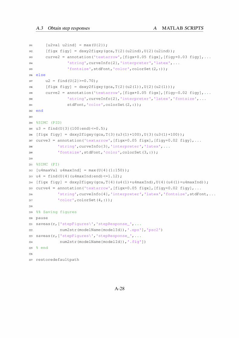
A.3 Obtain step responses A MATLAB SCRIPTS
191 [u2val u2ind] = max(U{2});
192 [figx figy] = dsxy2figxy(gca,T{2}(u2ind),U{2}(u2ind));
193 curve2 = annotation('textarrow',[figx+0.05 figx],[figy+0.03 figy],...
194 'string',curveInfo{2},'interpreter','latex',...
195 'fontsize',stdFont,'color',colorSet(2,:));
196 else
197 u2 = find(U{2}>=0.70);
198 [figx figy] = dsxy2figxy(gca,T{2}(u2(1)),U{2}(u2(1)));
199 curve2 = annotation('textarrow',[figx+0.05 figx],[figy−0.02 figy],...
200 'string',curveInfo{2},'interpreter','latex','fontsize',...
201 stdFont,'color',colorSet(2,:));
202 end
203
204 %SIMC (PID)
205 u3 = find(U{3}(100:end)<=0.5);
206 [figx figy] = dsxy2figxy(gca,T{3}(u3(1)+100),U{3}(u3(1)+100));
207 curve3 = annotation('textarrow',[figx+0.05 figx],[figy+0.02 figy],...
208 'string',curveInfo{3},'interpreter','latex',...
209 'fontsize',stdFont,'color',colorSet(3,:));
210
211 %SIMC (PI)
212 [u4maxVal u4maxInd] = max(U{4}(1:150));
213 u4 = find(U{4}(u4maxInd:end)<=1.12);
214 [figx figy] = dsxy2figxy(gca,T{4}(u4(1)+u4maxInd),U{4}(u4(1)+u4maxInd));
215 curve4 = annotation('textarrow',[figx+0.05 figx],[figy+0.02 figy],...
216 'string',curveInfo{4},'interpreter','latex','fontsize',stdFont,...
217 'color',colorSet(4,:));
218
219 %% Saving figures
220 pause
221 saveas(r,['stepFigures\','stepResponse_',...
222 num2str(modelName{modelId}),'.eps'],'psc2')
223 saveas(r,['stepFigures\','stepResponse_',...
224 num2str(modelName{modelId}),'.fig'])
225 % end
226
227 restoredefaultpath
A-28
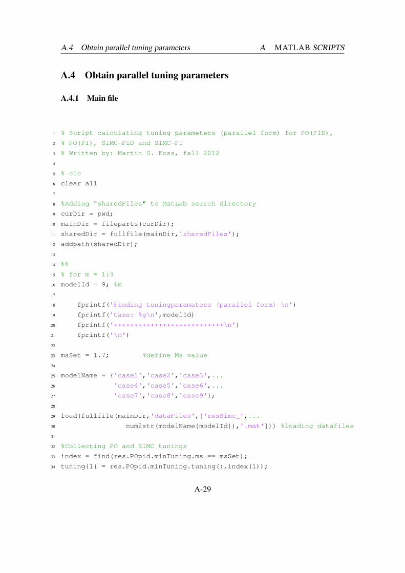
A.4 Obtain parallel tuning parameters A MATLAB SCRIPTS
A.4 Obtain parallel tuning parameters
A.4.1 Main file
1 % Script calculating tuning parameters (parallel form) for PO(PID),
2 % PO(PI), SIMC−PID and SIMC−PI3 % Written by: Martin S. Foss, fall 2012
4
5 % clc
6 clear all
7
8 %Adding "sharedFiles" to MatLab search directory
9 curDir = pwd;
10 mainDir = fileparts(curDir);
11 sharedDir = fullfile(mainDir,'sharedFiles');
12 addpath(sharedDir);
13
14 %%
15 % for m = 1:9
16 modelId = 9; %m
17
18 fprintf('Finding tuningparamaters (parallel form) \n')
19 fprintf('Case: %g\n',modelId)
20 fprintf('***************************\n')
21 fprintf('\n')
22
23 msSet = 1.7; %define Ms value
24
25 modelName = {'case1','case2','case3',...
26 'case4','case5','case6',...
27 'case7','case8','case9'};
28
29 load(fullfile(mainDir,'dataFiles',['resSimc_',...
30 num2str(modelName{modelId}),'.mat'])) %loading datafiles
31
32 %Collecting PO and SIMC tunings
33 index = find(res.POpid.minTuning.ms == msSet);
34 tuning{1} = res.POpid.minTuning.tuning(:,index(1));
A-29
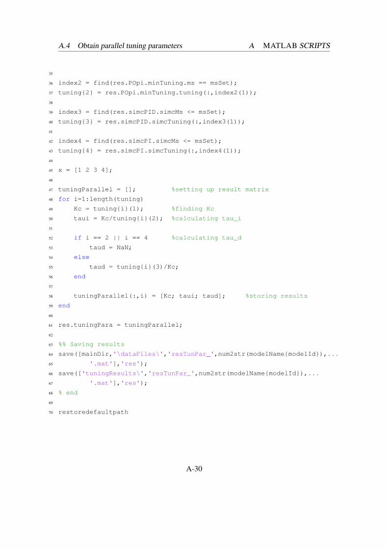
A.4 Obtain parallel tuning parameters A MATLAB SCRIPTS
35
36 index2 = find(res.POpi.minTuning.ms == msSet);
37 tuning{2} = res.POpi.minTuning.tuning(:,index2(1));
38
39 index3 = find(res.simcPID.simcMs <= msSet);
40 tuning{3} = res.simcPID.simcTuning(:,index3(1));
41
42 index4 = find(res.simcPI.simcMs <= msSet);
43 tuning{4} = res.simcPI.simcTuning(:,index4(1));
44
45 x = [1 2 3 4];
46
47 tuningParallel = []; %setting up result matrix
48 for i=1:length(tuning)
49 Kc = tuning{i}(1); %finding Kc
50 taui = Kc/tuning{i}(2); %calculating tau_i
51
52 if i == 2 || i == 4 %calculating tau_d
53 taud = NaN;
54 else
55 taud = tuning{i}(3)/Kc;
56 end
57
58 tuningParallel(:,i) = [Kc; taui; taud]; %storing results
59 end
60
61 res.tuningPara = tuningParallel;
62
63 %% Saving results
64 save([mainDir,'\dataFiles\','resTunPar_',num2str(modelName{modelId}),...
65 '.mat'],'res');
66 save(['tuningResults\','resTunPar_',num2str(modelName{modelId}),...
67 '.mat'],'res');
68 % end
69
70 restoredefaultpath
A-30
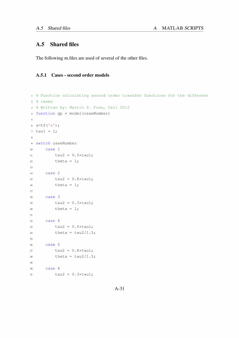
A.5 Shared files A MATLAB SCRIPTS
A.5 Shared files
The following m.files are used of several of the other files.
A.5.1 Cases - second order models
1 % Function calculating second order transfer functions for the different
2 % cases
3 % Written by: Martin S. Foss, fall 2012
4 function gp = model(caseNumber)
5
6 s=tf('s');
7 tau1 = 1;
8
9 switch caseNumber
10 case 1
11 tau2 = 0.5*tau1;
12 theta = 1;
13
14 case 2
15 tau2 = 0.8*tau1;
16 theta = 1;
17
18 case 3
19 tau2 = 0.3*tau1;
20 theta = 1;
21
22 case 4
23 tau2 = 0.5*tau1;
24 theta = tau2/1.5;
25
26 case 5
27 tau2 = 0.8*tau1;
28 theta = tau2/1.5;
29
30 case 6
31 tau2 = 0.3*tau1;
A-31
A.5 Shared files A MATLAB SCRIPTS
32 theta = tau2/1.5;
33
34 case 7
35 tau2 = 0.5*tau1;
36 theta = tau2/2;
37
38 case 8
39 tau2 = 0.8*tau1;
40 theta = tau2/2;
41
42 case 9
43 tau2 = 0.3*tau1;
44 theta = tau2/2;
45 end
46
47 gp = 1/((tau1*s+1)*(tau2*s+1));
48 gp.outputd = theta;
A.5.2 Cases - first order models
1 % Function calculating first order transfer functions, using the half rule,
2 % for the different cases
3 % Written by: Martin S. Foss, fall 2012
4 function gp = modelPI(caseNumber)
5
6 s=tf('s');
7 tau1 = 1;
8
9 switch caseNumber
10 case 1
11 tau2 = 0.5*tau1;
12 theta = 1;
13
14 case 2
15 tau2 = 0.8*tau1;
16 theta = 1;
17
18 case 3
A-32

A.5 Shared files A MATLAB SCRIPTS
19 tau2 = 0.3*tau1;
20 theta = 1;
21
22 case 4
23 tau2 = 0.5*tau1;
24 theta = tau2/1.5;
25
26 case 5
27 tau2 = 0.8*tau1;
28 theta = tau2/1.5;
29
30 case 6
31 tau2 = 0.3*tau1;
32 theta = tau2/1.5;
33
34 case 7
35 tau2 = 0.5*tau1;
36 theta = tau2/2;
37
38 case 8
39 tau2 = 0.8*tau1;
40 theta = tau2/2;
41
42 case 9
43 tau2 = 0.3*tau1;
44 theta = tau2/2;
45 end
46
47 Tau1 = tau1 + 0.5*tau2;
48 Theta = theta + 0.5*tau2;
49
50 gp = 1/(Tau1*s+1);
51 gp.outputd = Theta;
A.5.3 Controller
1 % function for generating the controller transferfunction
2 % on the form gc = K + I/s
A-33
A.5 Shared files A MATLAB SCRIPTS
3 % Written by: Martin S. Foss, fall 2012
4
5 function [gc gcPI varargout] = controller(K,I,D,taud,varargin)
6
7 s = tf('s');
8
9 if nargin == 3
10 gc = K + I/s + D*s; %PID Controller
11 elseif nargin == 2
12 gcPI = K + I/s; %PI controller
13 gc = NaN;
14 else
15 gc = K + I/s + (D*s)/(0.01*taud*s+1); %PID controller with
16 %derivative filter
17 end
18 return
A.5.4 Integral absolute error
1 function iae = iae(t,y)
2 % This is the function iae.m
3 % Simple integration routine made for computing IAE of time signal using
4 % trapez integration
5 % y − time signal vector
6 % t − time signal vector
7
8 % Initialize
9 i = 1;
10 npoints = length(t);
11 iae = zeros(1,size(y,2));
12
13 % Integrate
14 while i < npoints,
15 yavg = (y(i,:) + y(i+1,:))/2;
16 dt = t(i+1) − t(i);
17 int = abs(yavg)*dt;
18 iae = iae + int;
19 i = i + 1;
A-34

A.5 Shared files A MATLAB SCRIPTS
20 end
21
22 iae=iae';
23 return
A.5.5 Ms
1 % Function for calculating the Ms value
2 % written by: Chriss Grimholt 11 jan. 2012
3
4 function ms = ms(gp,gc)
5
6 ms = max(abs(freqresp(feedback(1,gp*gc),logspace(−4,4,40000))));7
8 return
A-35
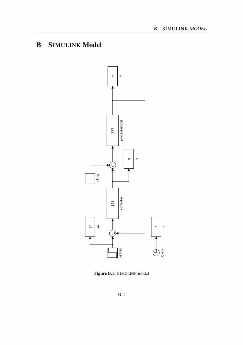
B SIMULINK MODEL
B SIMULINK Model
Figure B.1: SIMULINK model
B-1