NEW ORLEANS, LA

AUGUST 17, 2010

SPE-API Technical Luncheon:“Developing an Early-Warning System for

Well/Reservoir Problems”

Fred Goldsberry – WaveX ®

Chris Fair – Oilfield Data Services, Inc.

Outline

� Background: Data Acquisition & Processing� Data Measurement, Transfer and Visualization

� Virtual Rate Measurement

� The Wellbore-Completion-Reservoir System� PVT

� Heat Loading & Thermal Modeling

� Inflow Modeling

� Analysis/Evaluation Tools� PTA, RTA, Decline Analysis, p/z

� Nodal Analysis

� Reservoir Simulation

Outline II

� Creating an On-line Well Monitoring package� Take a batch process and make it continuous

� The Hard Parts in More Detail

� Wellbore Thermal and PVT Modeling

� Completion Model

� Reservoir Model (WaveX Reservoir Model)

� Don’t Forget the Coupled Effects

� Need to have a Closed Solution for Well Bore and Reservoir

� Effective Transient & Regime Recognition

� Combine steady-state and transient effects into same system of eqns

� Include Internal Checks for Validity

Outline III

� Examples of RT Process

� Conclusions

Data Acquisition: Instrumentation

� What do I really need to measure accurately?� Wellhead Pressure

� Wellhead Temperature (Thermowell)

� Flow Rates of Oil, Gas & Water

� Multiphase Meters, Venturi Meters, Turbine Meters

� Sep T & P

� Choke Setting

� Virtual Rate Measurement (VRM)

� Bottomhole Pressure

� Bottomhole Temperature

� Distributed Temperature

� NOTE: Last 3 not required for gas wells (still nice to have)

Data Acquisition: Pressure Gauges

� What to ask your gauge supplier:� What is the resolution (digital) or “effective resolution” for

Scada gauges?

� How many bits in the A/D converter?

� (Needs to be >14 for 1 psi resolution)

� How quickly can it sample or be polled?

� Is it thermally compensated? How much temperature change is required to cause the pressure to change 1 psi?

� Does the gauge measure and export its internal temperature?

� How susceptible is the gauge to plugging?

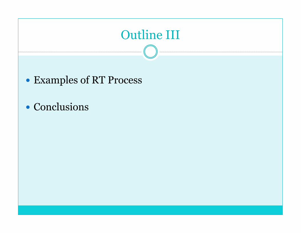
A/D Conversion: Scada/DCSResolution based on Scale and A/D Conversion

Resolution per bit (Bar)Resolution per bit (Bar)

Range (bar)Range (bar) 88 1212 1414 1818 2424

00--200200 0.781250.78125 0.0488280.048828 0.0122070.012207 0.0007630.000763 1.19E1.19E--0505

00--400400 1.56251.5625 0.0976560.097656 0.0244140.024414 0.0015260.001526 2.38E2.38E--0505

00--700700 2.7343752.734375 0.1708980.170898 0.0427250.042725 0.002670.00267 4.17E4.17E--0505

00--10001000 3.906253.90625 0.2441410.244141 0.0610350.061035 0.0038150.003815 5.96E5.96E--0505

Data Transfer: Don’t Lose Resolution!

� Before it gets to you, Your Data is likely to pass through:� One or two A/D converters

� An I/O card on the Control Panel

� Dead-band filters

� Signal filters

� Archive filters

� You can lose sampling resolution and instrument resolution at any point along the way

Data Visualization

Virtual Rate Measurement

� Used for Scenarios where there is not continuous rate measurement

� Common Instances:� Use productivity and periodic test sep rates

� Use choke settings and DPs

� Use WHT and Heat Loading model

� Allocation by Difference (Platform)

� Sonic

The Wellbore-Completion-Reservoir System

Governing Physics Laws & Rules

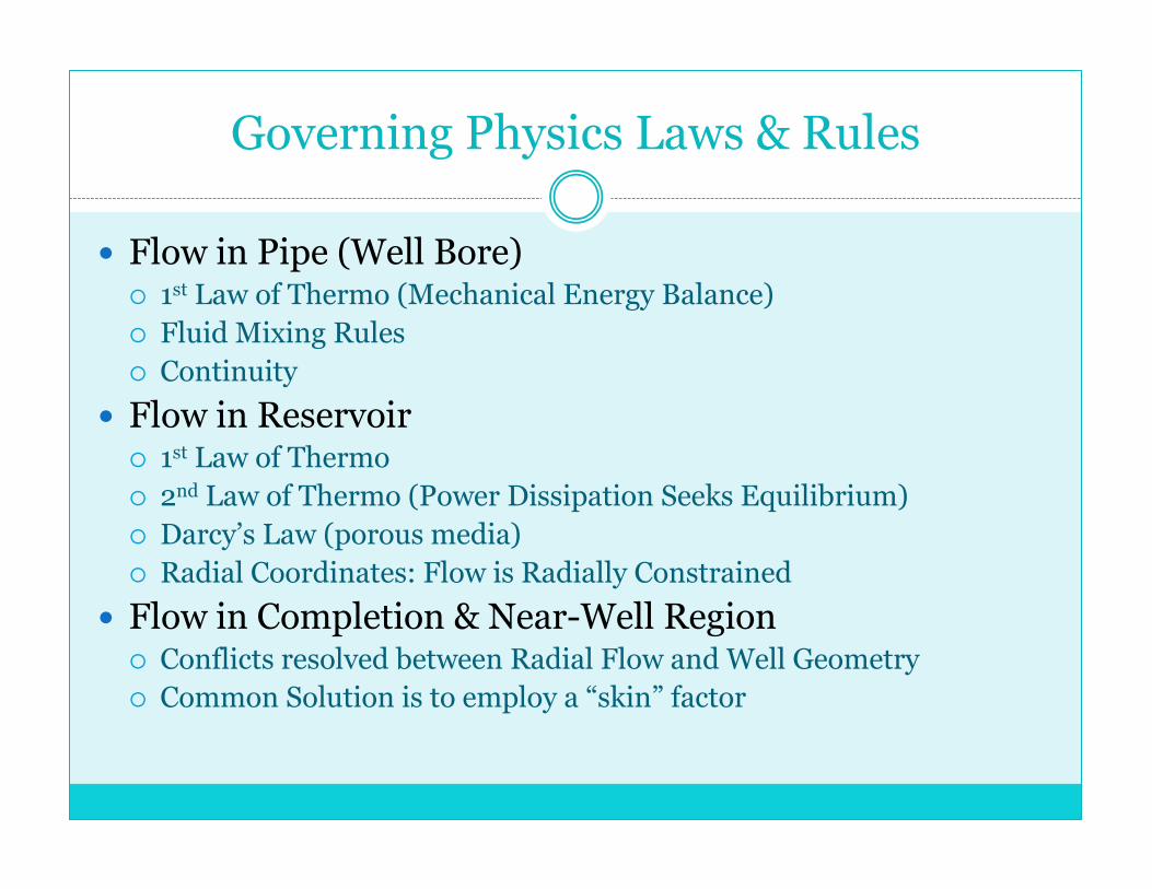
� Flow in Pipe (Well Bore) � 1st Law of Thermo (Mechanical Energy Balance)

� Fluid Mixing Rules

� Continuity

� Flow in Reservoir� 1st Law of Thermo

� 2nd Law of Thermo (Power Dissipation Seeks Equilibrium)

� Darcy’s Law (porous media)

� Radial Coordinates: Flow is Radially Constrained

� Flow in Completion & Near-Well Region� Conflicts resolved between Radial Flow and Well Geometry

� Common Solution is to employ a “skin” factor

Important Relationships For Multi-Phase Wells

� Well Bore� PVT Relationships

� Density

� Viscosity & Internal Energy

� Effective Friction Contribution

� Phase Interaction (Phase to Phase & Phase to Pipe BL)

� Rock & Fluid Interactions� Formation Compressibility and Elasticity (System Comp)

� Capillary Forces & Capillary Memory

� Threshold Pressure (Capillary Entry Pressure)

� Relative Permeability

� Inertial Forces

Other Complications

� Residence Time

� Joule-Thompson Cooling/Heating

� Partial Penetration/Perforation

� Pay Loss/Growth away from Completion

� Coupled Effects� Rate Surge/Decay

� Rate-Thermal

� Phase Blocking (Water Block, Condy Block)

� Rate-Thermal-Phase Effects

Residence Time

Rate Surges-Decays

Coupled Rate-Thermal Problem

� DHG responds “normally”

� WHP gauge responds differently

� WHP increases as DHGP decreases during flow

� Wellbore starts off “cool” & with higher inflow potential (flush production)

� Wellbore heats up, density decreases (head decreases)…mass flow rate decreases…which affects the heat loading…which affects the density…� And so on…and so on…

� Continues until the well reaches thermal equilibrium

Rate Surge #2

WHAT THEY ARE AND WHAT THEY TELL YOU

Analysis/Evaluation Tools

Analysis Types and Their Objectives

� PTA (Pressure Transient Analysis)� Skin, Perm, Deliverability, Communication, Productivity,

Reservoir Boundaries, Reserves

� RTA (Rate Transient Analysis)� Same as PTA, but with less reliability on boundaries

� Pres/z Plots (gas) & DPres Plots (oil)� Oil and/or Gas in Place

� Decline Analysis: Flowing BHP vs Time� Apparent Reserves – Running MBAL

� Inverse Productivity Analysis (DP/DQ vs Time)� Apparent Reserves – Running EBAL

Analysis/Evaluation Tools: PTA

� Build-up: After flowing the well for a while, shut it in and observe the pressure response

� Drawdown: After shutting in the well for a while, flow it on a constant choke and observe the pressure and rate response

� 2-rate: Change the rate enough to create a new transient; observe P & Q

� Multi-rate: Change the rates and compare DP vs Q

� Communication: Shut-in a well and see if a neighboring well causes the Pressure to drop

Analysis Type Examples

� Build-up PTA Derivative

� Drawdown PTA Semilog

� RTA

� P/z

� Decline Analysis (Running MBAL)

� IPA (Running EBAL)

Build-up PTA

Build-up Derivative Analysis

Drawdown - PTA

Drawdown PTA - Semilog Analysis

RTA Example - Cartesian

RTA – Semi-log Analysis

P/z Example

Decline Evaluation

IPA Example

Nodal Analysis

� Compares Reservoir Inflow (IPC) with Wellbore Performance (VLP)� Allows Prediction of DP to achieve a Rate (vice versa)

� Allows Prediction of Liquid Loading Scenarios

� Allows Optimization of Tubular Design

� Problems with Nodal� Infinite # of combos of skin & perm calculate the same rate

(Can’t use nodal to determine skin or perm)

� User has to pick the right inflow model and right VLP correlation

� Doesn’t handle transient situations well – may match your well today, but not next month

Nodal – IPC + VLP

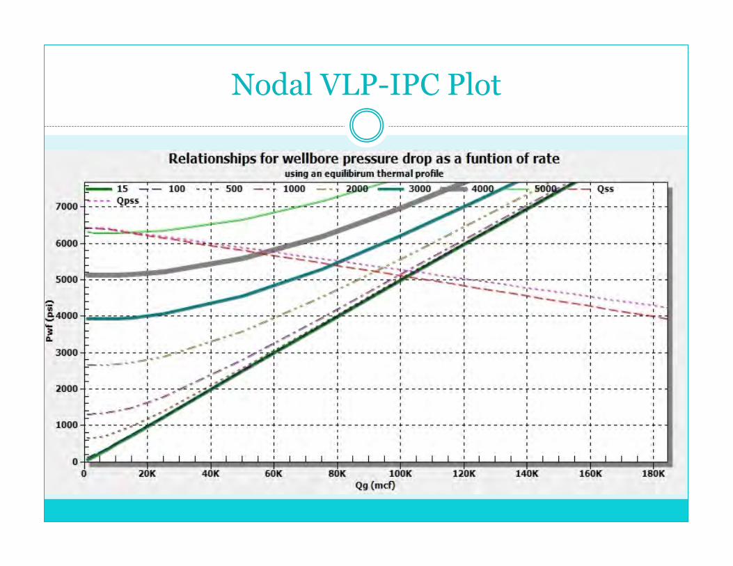
Nodal VLP-IPC Plot

Reservoir Simulation

� Tracks behavior (esp Pressure and Saturation) in the reservoir

� Incorporates Multiple Wells/Multiple Zones

� Matches History and Attempts to Predict Future Performance

� Coupled with a Wellbore Simulator, can do amazing things

� Drawback: It takes a while to run…but they’re getting faster

Simulation Gist…

Simulation: Well Grid

TAKE ALL THE BITS AND BOLT THEM TOGETHER

Components of a Real-Time Well Evaluation Package

What Do We Already Have? (Batch Process)

� Hopefully…adequate data frequency and quality

� “Snapshot” VLP

� “Snapshot” Inflow

� Reservoir Simulator

� Wellbore Model

� Geologic/Geo-Physical Model

� Enough Well History?

What Do We Need to Make it Real-Time?

� Link to RT Data (w/Validation of Data)

� Closed-Loop Wellbore Solution (w/Thermal Modeling)

� Closed-Loop Completion Solution - Can incorporate w/Reservoir Model

� Closed-Loop Reservoir Model

� Transient Recognition

� Regime Recognition

� Prediction vs. Actual Comparison

� Engineering by Difference (Did anything Change?)

The Bits…

Model Creation

and Validation

Reservoir Simulator

Real-Time Comparison toOverall System & Components of System

TransientNodal Analysis

Wellbore Modeling

Scada/DCSInterface

Integrated System ModelWellbore��������Completion��������Reservoir

Closed-Loop WB Components

� Wellbore Thermal Modeling (Warming/Cooling)

� Liquid Drop Out (Build-ups)

� Liquid Surge (Start-up)

� Phase Behaviour EOS Calcs� Use SRK or PR w/Peneloux

� Rate Modeling� Residence Time

� Rate Surging & Decay

� Coupled Effects (Rate-Thermal-Phase)

Developing Thermal/PVT Models

� Run Static Temp/Pressure Survey

� Run Flowing Temp/Pressure Survey� Multiple Rates

� Develop Heat Transfer Model – Account for:� Heat Capacity of Fluids/Tubulars/Annuli/Sinks

� Heat X-fer via Conduction

� Heat X-fer via Convection

� Heat X-fer via Forced Convection

� Can Tune PVT using same data…just get a good sample first

Continuity Equation

� Rate of Change in Density Caused by Changes in Mass Flux

)( vt

ρρ

•∇−=∂

∂

Differential Form of Bernoulli EqnCompressible Conditions

0)()(

/)(

2

2

12

2

1

2

1

2

2

1

=+

+++∆+∆

∑∑

∫

iviii RL

p

p

evfv

Wsdphgv

h

ρ

Mechanical Energy Balance (Bernoulli Equation)

� For Single-Phase Gas Flow in Pipes, the MEB reduces to:

dp/ρ = -(g sin θ/gc + 2ff u2/gc D) dL

� Basis for CS, Gray & A-C

Bernoulli for Single Phase OilIncompressible Conditions

� Basis for Hagedorn-Brown & Beggs/Brill

02

2

=++++ s

c

f

c

dWDg

dLvfdz

g

g

cgvdv

d

dp

ρ

Bernoulli Solution Process

Build Parametric Models

Assume Continuity

Solve Bernoulli (MEB)

Check Continuity

Note: If Continuity Doesn’t Hold, the Well is Loading–up (which is important to know)

Using a Direct Bernoulli Solution for WB

� Works for Oil, Gas or Water (Continuity)

� Gas� Have DP, solve for rate

� Have Rate, solve for DP

� Oil� Have Rate, solve for Water cut

� Have DP, solve for Water cut

� Much Easier to Apply Parametric Models:� Thermal Transients

� Rate Transients

� Phase Transients

� Combined Rate, Phase & Thermal Transients

Completion Modeling

� Reconcile Well Geometry (frac, horizontal, etc.) with base inflow� Build Dual Perm Model

� Build “skin” model (easiest way if it works)

� Reconcile Completion/Reservoir Interaction� Partial Perforation/Penetration

� Pay Loss/Growth

� Near Well Stresses – Elasto-Plastic Rock

� True “Afterflow” vs. Terminal Velocity Flow

Closed-Loop Reservoir Solution

� Dr. Fred…Wavex Theory

� Focus on fact that it’s the same sol’n as conventional in radial flow and in PSS flow, but has a banded regime solution during post-boundary transient flow

Boundary Contact Types

� Dr. Fred talks about boundary contact types, especially gas-water contacts and fizzy oil-water contacts

Results of the WaveX Method…

� A Closed Solution

� Running Volumetrics – don’t have to reach PSS to get a volume

� More Accurate Permeability-Thickness

� More Accurate Distances to Limits

� Differentiate between Faults, Strat-outs & Gas-Liquid Contacts

� Relative Position of Limits to Each Other

� A Map You can show the G&G guys without getting laughed out of the room

Closed Solution – Volumetrics & Geometry

SMI 109

No. A-1

Anomally 508'-549'

622'

1,345'

1,736' 1,969'

2,784'

Rin

v =

3,2

15

'

Scale: 1" = 1,000'

154'

WAVEX Energy Map

1-2-3-4 Limit Rotation

En

erg

y W

idth

1,7

98

'

SM

I 109

No

. A

-1

An

om

ally 5

08'-549'

622'

1,3

45'

1,7

36'

1,9

69'

2,7

84'

Rinv = 3,215'

Scale

: 1"

= 1

,000'

154'

WA

VE

X

En

erg

y M

ap

1-2

-3-4

Lim

it R

ota

tio

n

Energy Width 1,798'

SMI 109

No. A-1

Anomally 508'-549'

622'

1,345'

1,736' 1,969'

2,784'R

inv =

3,2

15

'

Scale: 1" = 1,000'

154'

WAVEX Energy Map

1-2-3-4 Limit Rotation

En

erg

y W

idth

1,7

98'

Boundary Contact Typing: H2O Contact

Transient and Regime Recognition

� Locate New Transients� Rate goes to zero, Rate stops being zero

� Rate changes enough to start new transient

� Pressure Methods

� Wavelets

� De-convolution Variance

� DP Logic

� Banded Response Recognition� Transient vs. Steady-State

� Boundary Recognition

� Transition Recognition

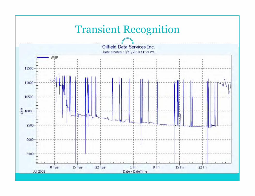
Transient Recognition

ERROR: stackunderflow

OFFENDING COMMAND: ~

STACK: