Embed Size (px)
Citation preview
Faculteit Bio-ingenieurswetenschappen
Academiejaar 2015-2016
Spatio-temporal modelling of filter cake
formation in filtration processes
Bram De Jaegher
Promotor: Prof. dr. ir. Ingmar Nopens & dr. ir. Jan Baetens
Tutor: ir. Wouter Naessens
Masterproef voorgedragen tot het behalen van de graad van
Master in de bio-ingenieurswetenschappen: Chemie en bioprocestechnologie
De auteur en promotor geven de toelating deze scriptie voor consultatie beschikbaar te stellen
en delen ervan te kopieren voor persoonlijk gebruik. Elk ander gebruik valt onder de beperkin-
gen van het auteursrecht, in het bijzonder met betrekking tot de verplichting uitdrukkelijk de
bron te vermelden bij het aanhalen van resultaten uit deze scriptie.
The author and promoter give the permission to use this thesis for consultation and to copy
parts of it for personal use. Every other use is subject to the copyright laws, more specifically
the source must be extensively specified when using results from this thesis.
Ghent, June 3, 2016
The promoters,
Prof. dr. ir. Ingmar Nopens dr. ir. Jan Baetens
The tutor, The author,
ir. Wouter Naessens Bram De Jaegher
Acknowledgement
It all started with a bright summer’s day in August when I timidly entered the simulation lab
of the notorious department of Mathematical Modelling, Statistics and Bioinformatics. Now,
ten months later, I can proudly present this master thesis. Despite the vast amount of work
and the various complaints of my computer, I can confidently say that I consider this year as
a very positive and enriching period of my student career. However, the result of this master
dissertation would not have been the same without a few people and therefore I would like
to pay them my respects.
First of all, thank you Ingmar Nopens and Jan Baetens for your supervision and thorough
corrections. Second of all, I would like to thank Wouter Naessens for being an awesome su-
pervisor and providing guidance throughout this thesis. I am truly sorry for the hour-long,
brain frying discussions on the force balance and the heavy workload I put on your shoulders
during the first and last weeks. Michael Ghijs, for showing me the relativeness of deadlines
and the relevance of the Beatles in data storage. May the lift force be with you!
On a more serious note, thank you Timothy Van Daele for helping me with all my Open-
FOAM, LaTeX and Github questions and good luck with the finalisation of your PhD. Stijn
Van Hoey, for aiding me with the MATLAB, Github and Linux related questions. Next, a spe-
cial notification for my fellow simulation lab thesis friends; Arthur, Laurentijn, Sofie, Annelies
and Bavo for the occasional lighthearted chat and all members BIOMATH and KERMIT for
the friendly and welcoming environment. Muchas gracias Jose por los datiles.
On a more personal note, a special thanks to my girlfriend, Nancy, for the corrections, support
and for being an amazing person. My parents, for all their unconditional support. Finally, I
would like to thank “Wa boel e da ier?” for all the great experiences during these five years
at ’t Boerekot and I wish you all the best of luck.
i

ii

Summary
At present time, membrane filtration processes suffer from a high operational cost due to
fouling abatement measures. The description of fouling mechanisms is still highly empirical
and does not provide an adequate framework for the development of decision support tools to
aid a cost-effective operation of these processes. The objective of this master dissertation is
the development and evaluation of a spatio-temporal model to describe particle behaviour in
a realistic and accurate manner in order to unravel the mechanisms of filter cake formation.
This model aims to pinpoint the most influential processes that should be included in the
next generation of decision support tools for filtration processes.
In the context of this dissertation, a literature review was performed to identify the cur-
rent fouling modelling approaches and to provide a overview of the available profilometric
techniques for the calibration and validation of the model under development. The filter
cake formation model of Ghijs (2014) was further extended to a three-dimensional model,
the representation of the feed flow was extended to multidisperse suspensions, a new and
highly efficient collision detection algorithm was implemented and a user-friendly graphical
user interface was developed for the analysis of the simulation results.
A laboratory scale microfiltration device was designed with computational fluid dynamics
for the calibration/validation of the model and a qualitative validation, based on the Segre-
Silberberg effect, was performed. The latter indicated some imperfections in the force balance
on the flowing particles. A scenario analysis was carried out to assess the behaviour of the
model under various operational conditions.
The simulations and qualitative validation led to a clear understanding of some of the mod-
elling deficits and shortcomings, such as the formation of narrow filter cake patches and the
absence of appropriate wall repulsion effects. Still, with an eye on the future development of
the model, guidelines are provided to resolve these issues.
In the end, it can be concluded that a lot of progression was made towards a realistic rep-
resentation of filter cake formation processes. Furthermore, a lot of knowledge was gained
concerning their underlying mechanisms which was, after all, the main objective of this master
thesis.
iii

iv

Samenvatting
Momenteel hebben membraanfiltratieprocessen een grote operationele kost die vooral te wij-
ten is aan de genomen maatregelen tegen de vervuiling van het membraan. De beschrijving
van deze vervuilingsmechanismen is nog steeds zeer empirisch en biedt geen goed kader voor de
ontwikkeling van beslissingsondersteunende systemen. Deze systemen kunnen onder andere
de kosteneffectiviteit van deze processen verbeteren. Het doel van deze thesis is de ont-
wikkeling en evaluatie van een spatio-temporeel model dat het gedrag van gesuspendeerde
partikels in een filtratiesysteem op een realistische en accurate manier kan beschrijven. Dit
model kan waardevolle inzichten leveren in de belangrijkste onderliggende mechanismen van
filterkoekvorming. Deze mechanismen kunnen dan opgenomen worden in de volgende gene-
ratie aan beslissingsondersteunende systemen.
In het kader van dit proefschrift werd een literatuuronderzoek uitgevoerd dat een overzicht
biedt van de huidige membraanvervuilingsmodellen. Tevens wordt een overzicht gegeven van
de beschikbare profilometrische technieken voor de kalibratie en validatie van het model in
ontwikkeling. Het spatio-temporeel model van Ghijs (2014), dat de filterkoekvorming be-
schrijft in membraanbioreactoren, werd verder uitgebouwd naar een driedimensionaal model.
Een polydisperse voorstelling van de disperse fase werd bewerkstelligd en een nieuw en efficient
collisiedetectie-algoritme werd geımplementeerd. Voor de analyse van de simulatieresultaten
werd een gebruiksvriendelijke grafische gebruiksomgeving ontwikkeld.
Een microfiltratie pilootopstelling werd ontwikkeld via numerieke stromingsleer voor de kali-
bratie/validatie van het model en een kwalitatieve validatie werd uitgevoerd op basis van het
Segre-Silberberg effect. Dit laatste toonde een aantal onvolmaaktheden aan in de krachten-
balans over de gesuspendeerde partikels. Vervolgens werd een scenarioanalyse uitgevoerd om
het gedrag van het model onder verschillende operationele condities te evalueren.
De simulatieresultaten en kwalitatieve validatie hebben geleid tot een duidelijk inzicht in
enkele tekortkomingen van het model zoals de vorming van smalle filterkoektorens en de
afwezigheid van de gepaste wandrepulsie-effecten. Met het oog op de toekomstige ontwikkeling
van het model werden een aantal richtlijnen verschaft om deze kwesties aan te pakken. Er
kan besloten worden dat er veel vooruitgang geboekt is naar een realistische voorstelling van
filterkoekvormende processen, waarbij veel inzicht verworven is in de onderliggende mecha-
nismen; het uiteindelijke hoofddoel van deze dissertatie.
v

vi

Contents
Acknowledgement i
Summary iii
Samenvatting v
Contents viii
List of Symbols ix
List of Abbreviations xiii
1 Introduction 1
1.1 Introduction . . . . . . . . . . . . . . . . . . . . . . . . . . . . . . . . . . . . . 1
1.2 Problem statement . . . . . . . . . . . . . . . . . . . . . . . . . . . . . . . . . 2
1.3 Objectives of this research . . . . . . . . . . . . . . . . . . . . . . . . . . . . . 3
1.4 Outline: the roadmap through this dissertation . . . . . . . . . . . . . . . . . 3
2 Literature Review 5
2.1 Membrane fouling . . . . . . . . . . . . . . . . . . . . . . . . . . . . . . . . . 5
2.2 Membrane fouling models . . . . . . . . . . . . . . . . . . . . . . . . . . . . . 6
2.2.1 Resistance-in-series models . . . . . . . . . . . . . . . . . . . . . . . . 7
2.2.2 Advanced mechanistic models . . . . . . . . . . . . . . . . . . . . . . . 8
2.2.3 Data-driven models . . . . . . . . . . . . . . . . . . . . . . . . . . . . 19
2.3 Profilometry . . . . . . . . . . . . . . . . . . . . . . . . . . . . . . . . . . . . . 22
2.3.1 Non-optical methods . . . . . . . . . . . . . . . . . . . . . . . . . . . . 22
2.3.2 Optical methods . . . . . . . . . . . . . . . . . . . . . . . . . . . . . . 23
3 Spatio-temporal model of filter cake formation 27
3.1 Assumptions . . . . . . . . . . . . . . . . . . . . . . . . . . . . . . . . . . . . 28
3.2 Dispersed phase . . . . . . . . . . . . . . . . . . . . . . . . . . . . . . . . . . 29
3.3 Filter cake formation . . . . . . . . . . . . . . . . . . . . . . . . . . . . . . . . 31
3.4 Continuous phase . . . . . . . . . . . . . . . . . . . . . . . . . . . . . . . . . . 31
vii

3.4.1 Fluid dynamics . . . . . . . . . . . . . . . . . . . . . . . . . . . . . . . 31
3.4.2 Computational fluid dynamics . . . . . . . . . . . . . . . . . . . . . . 33
4 Model development 35
4.1 Polydispersity . . . . . . . . . . . . . . . . . . . . . . . . . . . . . . . . . . . . 35
4.1.1 Particle sampling . . . . . . . . . . . . . . . . . . . . . . . . . . . . . 36
4.1.2 Filter cake formation . . . . . . . . . . . . . . . . . . . . . . . . . . . 38
4.2 Extension to a three-dimensional model . . . . . . . . . . . . . . . . . . . . . 40
4.3 Parallelisation . . . . . . . . . . . . . . . . . . . . . . . . . . . . . . . . . . . 41
4.4 Model architecture . . . . . . . . . . . . . . . . . . . . . . . . . . . . . . . . . 41
4.5 Software . . . . . . . . . . . . . . . . . . . . . . . . . . . . . . . . . . . . . . . 43
4.5.1 MATLAB . . . . . . . . . . . . . . . . . . . . . . . . . . . . . . . . . . 43
4.5.2 Python . . . . . . . . . . . . . . . . . . . . . . . . . . . . . . . . . . . 43
4.5.3 SALOME . . . . . . . . . . . . . . . . . . . . . . . . . . . . . . . . . . 44
4.5.4 OpenFOAM . . . . . . . . . . . . . . . . . . . . . . . . . . . . . . . . 44
4.6 Post-processing user interface . . . . . . . . . . . . . . . . . . . . . . . . . . . 44
5 Results and discussion 47
5.1 Calibration and validation: model-based design of a filtration unit . . . . . . 47
5.2 Case studies . . . . . . . . . . . . . . . . . . . . . . . . . . . . . . . . . . . . . 52
5.2.1 Setup . . . . . . . . . . . . . . . . . . . . . . . . . . . . . . . . . . . . 52
5.2.2 Mesh independence of the continuous phase . . . . . . . . . . . . . . 55
5.2.3 The Segre-Silberberg effect: a qualitative validation . . . . . . . . . . 57
5.2.4 Mesh independency of the agent-based model . . . . . . . . . . . . . . 61
5.2.5 Spatial segregation of the suspended particles . . . . . . . . . . . . . 61
5.2.6 Effect of polydispersity . . . . . . . . . . . . . . . . . . . . . . . . . . 63
6 General discussion and perspectives 65
6.1 Remarks on the bulk phase force balance . . . . . . . . . . . . . . . . . . . . 65
6.2 Filter cake formation . . . . . . . . . . . . . . . . . . . . . . . . . . . . . . . 66
6.3 Coupling ABM and continuous model . . . . . . . . . . . . . . . . . . . . . . 67
6.4 Sources of numerical instability . . . . . . . . . . . . . . . . . . . . . . . . . . 69
6.5 Profilometry . . . . . . . . . . . . . . . . . . . . . . . . . . . . . . . . . . . . . 69
7 Conclusion 71
Bibliography 73
A Appendix: Technical drawing microfilter 81
viii

List of Symbols
Symbol Description Unit
A inlet area [m2 ]
Am membrane area [m2 ]
α specific filtration resistance [m kg −1]
cb bulk concentration [kg m −3]
cbc bulk concentration of particles that are retained on the
membrane surface
[kg m −3]
cbm the mass concentration of particles able to penetrate the
membrane
[kg m−3]
cc mass concentration of the cake layer [kg m −3]
cm concentration on membrane surface [kg m −3]
Dh hydraulic diameter [m ]
dp particle diameter [m ]
dp mean diameter of bulk particles [m ]
∆i thickness of a filter cake slice [m ]
∆p pressure drop [Pa ]
∆pc pressure drop over cake layer [Pa ]
∆pt,eff the effective transmembrane pressure acting on the
membrane surface
[Pa ]
∆t time step [s ]
E probability of deposition [ - ]
ε actual filter cake porosity [ - ]
εm membrane porosity [ - ]
εsph filter cake porosity for perfect spheres [ - ]
ix

Symbol Description Unit
~Fam added mass force [N ]~Farch Archimedes force [N ]~Fbody body forces [N ]~Fdrag drag force [N ]~Fg gravitational force [N ]~Fhist history force [N ]~Fhydr resulting hydrodynamic force [N ]~Flift lift force [N ]~Fp pressure gradient induced force [N ]~Fsurf surface forces [N ]
FA adhesion force [N ]
Fd drag force [N ]
Fg gravity force [N ]
Fi interparticle force [N ]
Fl lift force [N ]
FN normal force [N ]
Fnum particle size distribution [ - ]
Ft tangential shear stress [N ]
Fτ friction force [N ]
f external body forces [N m −1]
fc friction factor [ - ]
gb particle size distribution of the bulk particles [ - ]
gcake particle size distribution of the particles retained by the
membrane
[ - ]
gm particle size distribution of the particles able to enter
the pores
[ - ]
J flux [m3 m−2 s −1]
K Kozeny constant [ - ]
Kc specific cake resistance [m−2]
Kd rate coefficient of sludge detachment [s −1]
Kp membrane specific constant [m−1]
κ fluid velocity gradient [ s −1]
k adhesion parameter [ s m −1]
kc model parameter cake layer [m2 kg −1]
kf model parameter fouling [ - ]
x
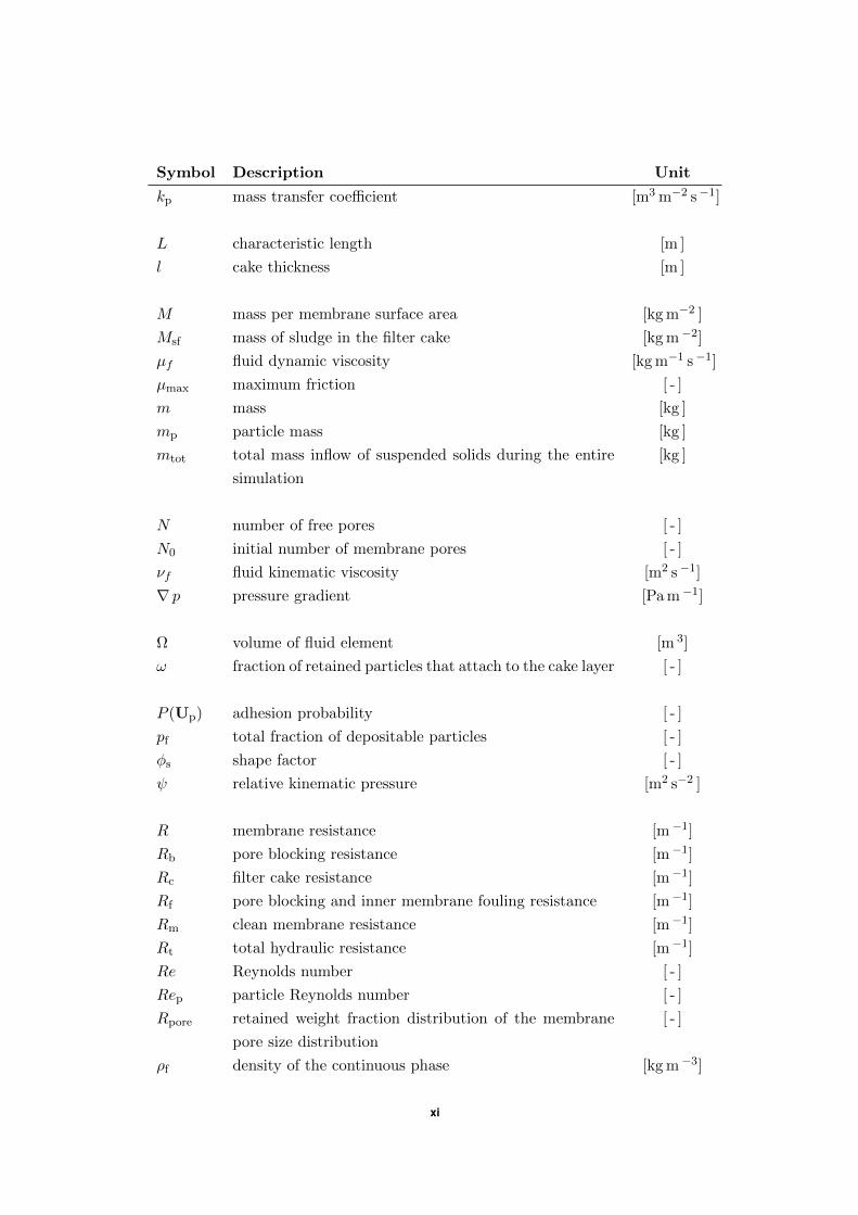
Symbol Description Unit
kp mass transfer coefficient [m3 m−2 s −1]
L characteristic length [m ]
l cake thickness [m ]
M mass per membrane surface area [kg m−2 ]
Msf mass of sludge in the filter cake [kg m −2]
µf fluid dynamic viscosity [kg m−1 s −1]
µmax maximum friction [ - ]
m mass [kg ]
mp particle mass [kg ]
mtot total mass inflow of suspended solids during the entire
simulation
[kg ]
N number of free pores [ - ]
N0 initial number of membrane pores [ - ]
νf fluid kinematic viscosity [m2 s −1]
∇ p pressure gradient [Pa m −1]
Ω volume of fluid element [m 3]
ω fraction of retained particles that attach to the cake layer [ - ]
P (Up) adhesion probability [ - ]
pf total fraction of depositable particles [ - ]
φs shape factor [ - ]
ψ relative kinematic pressure [m2 s−2 ]
R membrane resistance [m −1]
Rb pore blocking resistance [m −1]
Rc filter cake resistance [m −1]
Rf pore blocking and inner membrane fouling resistance [m −1]
Rm clean membrane resistance [m −1]
Rt total hydraulic resistance [m −1]
Re Reynolds number [ - ]
Rep particle Reynolds number [ - ]
Rpore retained weight fraction distribution of the membrane
pore size distribution
[ - ]
ρf density of the continuous phase [kg m −3]
xi

Symbol Description Unit
ρp,m the density of particles in the membrane pores [kg m−3]
ρs density of the bulk particles [kg m −3]
S specific surface area [m2 ]
Sf model parameter fouling saturation [ - ]
Si specific surface area of the particles [m2 ]
t time [s ]
tf filtration time/cycle [s ]
ttot total simulation time [s ]
τ viscous stress tensor [N ]
τW shear stress [Pa ]
θ angle of friction [ - ]
θc critical friction angle [ - ]
Uc fluid velocity [m s −1]
Ucf cross-flow velocity [m s −1]
Um maximum channel velocity [m s −1]
Up particle velocity [m s −1]
Ur relative particle velocity [m s −1]
Ur,eff Faxen corrected relative velocity [m s −1]
Vp particle volume [m 3]
Vm total membrane volume [m 3]
Vp,m volume of particles that sediment each filtration cycle [m 3]
v velocity [m s −1]
vd diffusion velocity [m s −1]
vg gravitational sedimentation velocity [m s −1]
vi particle interaction velocity [m s −1]
vl inertia lifting velocity [m s −1]
vs shear induced diffusion velocity [m s −1]
vtot total backtransport velocity [m s −1]
xii

List of Abbreviations
ABM agent-based model
AFM atomic force microscopy
API application programming interface
CAD computer-aided design
CDF cumulative distribution function
CFD computational fluid dynamics
CLSM confocal laser scanning microscopy
DHM digital holographic microscopy
DICM differential interference contrast microscopy
DLVO Derjaguin, Landau, Verwey and Overbeek
FEM finite element method
FP Fourier profilometry
FPP fringe projection profilometry
FVM finite volume method
GUI graphical user interface
MBR membrane bioreactor
MP Moire profilometry
OCT optical coherence tomography
PDE partial differential equation
xiii

PMF probability mass function
PSD particle size distribution
RIS resistance-in-series
SCR simulation time to computational time ratio
SEM scanning electron microscopy
SP stylus profilometry
SS suspended solids
STM scanning tunneling microscopy
TMP transmembrane pressure
WLAC white light axial chromatism
WLI white light interferometry
xiv
CHAPTER 1Problem statement, research objectives
1.1 Introduction
Membrane filtration is a purely physical separation process where a suspension is drawn
through a semi-permeable membrane and the suspended constituents larger than the mem-
brane pores are retained. In descending pore size, a distinction is made between microfiltra-
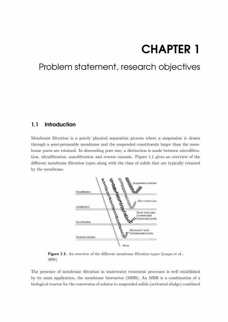
tion, ultrafiltration, nanofiltration and reverse osmosis. Figure 1.1 gives an overview of the
different membrane filtration types along with the class of solids that are typically retained
by the membrane.
Figure 1.1: An overview of the different membrane filtration types (Luque et al.,
2008).
The presence of membrane filtration in wastewater treatment processes is well established
by its main application, the membrane bioreactor (MBR). An MBR is a combination of a
biological reactor for the conversion of solutes to suspended solids (activated sludge) combined

2 1.2 PROBLEM STATEMENT
with a membrane filter to remove these solids and thereby produce clean water (Judd, 2011).
Membrane filtration replaces the traditional, gravitational sedimentation of activated sludge
and produces water with a significantly higher quality (Judd, 2008). Moreover, MBRs are
more robust and are able to handle higher concentrations of suspended solid, leading to
a higher loading capacity and consequently more compact treatment plants. Other, more
exotic, applications of membrane filtration in wastewater treatment are, among others, the
removal of emulsified oils and the recovery of heavy metals (Fu and Wang, 2011; Cheryan and
Rajagopalan, 1998).
Nowadays, membrane filtration is also being employed in a vast range of industrial, medical
and biotechnological processes and the market of membrane filtration is ever growing (Scott
and Highes, 2012; Luque et al., 2008). Important applications of membrane filtration can
be found in the paper production industry for lignosulfonate fractionation and color removal
(Luque et al., 2008), in the food industry for the clarification of beer, wine and vinegar
(Cimini et al., 2013; Ulbricht et al., 2009; Tamime, 2012), in the medical sector for the
continuous filtration of blood plasma and in biotechnology for the clarification of fermentation
broth (Homsy et al., 2012; Prasad, 2010). Several potential uses for membrane filtration
in renewable energy applications, such as biogas upgrading and biodiesel purification, are
proposed in literature (Charcosset, 2014; Dube et al., 2007). In short, membrane filtration
has become indispensable in industrial as well as wastewater treatment processes.
There is, nonetheless, a major disadvantage coupled with membrane filtration, i.e. membrane
fouling. The continuous feed and retention of suspended solids leads to the formation of
fouling layers on top (filter cake) or inside the membrane and increases the resistance towards
liquid permeation. Hence, operation of a membrane filtration unit requires continuous fouling
control which includes backwashing, aeration and chemical cleaning of the membrane. These
procedures are not able to fully regenerate the membrane due to irrecoverable fouling, leading
to the insuperable decay of the membrane. The effectuation of fouling control measures
and the replacement of membranes gives rise to considerable operational expenses, making
membrane filtration a costly technique (Owen et al., 1995).
1.2 Problem statement
In spite of the growing importance of membrane filtration in industry and wastewater treat-
ment processes, there is still little understanding of the underlying processes of membrane
filtration. In order to suppress fouling and prolong the lifetime of pressure-driven membrane
systems as much as possible, the operation is highly conservative. Fouling remediation pro-
cedures are performed frequently, leading to a sub-optimal operation which is costly and
inefficient both from an energetic and material perspective. Quite some efforts have been put
in fouling research, but there is still poor insight in the system dynamics. Efforts to model
membrane filtration and the fouling build-up are mostly empirical and typically based on

CHAPTER 1 INTRODUCTION 3
the resistance-in-series (RIS) approach (Section 2.2.1). Such models are capable of accurately
predicting flux decline and transmembrane pressure (TMP) increase over time, but only under
the specific operational conditions for which they are calibrated. Hence, they lack extrapo-
lation capacity to accurately predict fouling rates and optimal backflushing frequencies in a
general setting. Moreover, RIS models are often overparameterised and require frequent re-
calibration with a vast amount of data for accurate parameter estimations, making real-time
recalibration typically not feasable.
These reasons have led to the fact that efforts have not yet resulted in a universally applicable
membrane filtration model, neither do they agree on fundamental fouling principles. An
in-depth understanding of the underlying fouling processes will allow for a more responsive,
dynamic operation and a better design of filtration installations. Furthermore, the availability
of accurate and robust fouling models will enable the implementation of more advanced control
strategies, such as internal model control, model-based predictive control, or in silico tuning
of process controllers.
1.3 Objectives of this research
The first objective of this master thesis is the extension of the mechanistic, spatially explicit
modelling framework proposed by Ghijs (2014). The model has its limitations and will be
critically analysed, extended and polished, so to progress towards a physically more accurate
description of all relevant processes contributing to filter cake formation.
The second objective is the model-based design and realisation of a laboratory scale membrane
filtration system for the calibration and validation of the abovementioned model.
It should be kept clear at all times that the purpose of this model is not the real-time
evaluation of operational conditions, but rather unraveling fouling mechanisms. Hopefully,
this model will be able to provide valuable insights into the key mechanisms of membrane
fouling needed for the future development of computationally efficient filtration models for
dynamic control, backflushing prediction, computer-aided design (CAD), etc.
1.4 Outline: the roadmap through this dissertation
This dissertation starts with a literature review of membrane fouling models and profilometric
techniques. Chapter 3 provides a description of the model developed by Ghijs (2014). The
improvements of this model, performed in this thesis, are discussed in Chapter 4. Next, the
results of a qualitative validation of the improved model and a scenario analysis are elucidated
in Chapter 5. Chapter 6 addresses the modelling imperfections and provides guidelines for the
future development of the model. Finally, this master dissertation presents the conclusions
in Chapter 7.


CHAPTER 2Literature Review
In order to further develop and improve the spatio-temporal model of filter cake formation
elaborated by Ghijs (2014), it is necessary to thoroughly review the various modelling ap-
proaches in literature. In this manner, all processes and accompanying interdependencies can
be mapped out, which enables the development of a realistic model comprising all relevant
processes. The first part of this chapter is dedicated to this. In the second part of this chapter,
a few promising profilometric techniques, necessary for model calibration, will be discussed.
2.1 Membrane fouling
Membrane fouling comes in many forms and types. Furthermore, generally accepted mem-
brane fouling terminology is altered by different authors in the field. Before exploring the
different models, some important concepts and the associated lexicon will be defined.
Mohammadi et al. (2003) defines membrane fouling as “ [...] the existence and growth of
micro-organisms and the irreversible collection of materials on the membrane surface which
results in a flux decline.” However, a more suitable definition is “ [...] the process resulting in
loss of performance of a membrane due to deposition of suspended or dissolved substances on
its external surfaces, at its pore openings, or within its pores” by Koros et al. (1996) because
it also includes pore fouling.
Depending on the type of membrane filtration (nanofiltration, microfiltration, etc. ), different
types of fouling can be encountered during operation. Generally, fouling can be classified as
follows:
• scaling: precipitation of substances due to exceeding the solubility product induced by
the process of concentration polarisation;
• particulate fouling, inorganic and organic;
6 2.2 MEMBRANE FOULING MODELS
• biofouling: fouling effects due to colonisation by bacteria;
• fouling by macromolecular substances;
• chemical reaction of solutes with the membrane polymer and/or its boundary layer;
It is nevertheless important to keep in mind that these are only the main types. It is possible
that other, more specific types exist. Some authors prefer to classify fouling in terms of
persistency (reversible, irreversible and irrecoverable fouling) whilst others favor a mechanical
categorisation (pore blocking, cake formation, intermediate blocking, etc. ). Unfortunately,
these classifications cannot be compared mutually, as there is no complete parity between any
of these types.
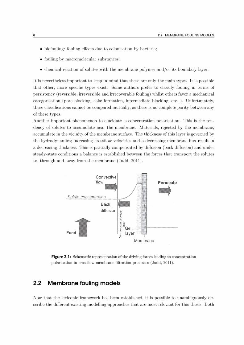
Another important phenomenon to elucidate is concentration polarisation. This is the ten-
dency of solutes to accumulate near the membrane. Materials, rejected by the membrane,
accumulate in the vicinity of the membrane surface. The thickness of this layer is governed by
the hydrodynamics; increasing crossflow velocities and a decreasing membrane flux result in
a decreasing thickness. This is partially compensated by diffusion (back diffusion) and under
steady-state conditions a balance is established between the forces that transport the solutes
to, through and away from the membrane (Judd, 2011).
Figure 2.1: Schematic representation of the driving forces leading to concentration
polarisation in crossflow membrane filtration processes (Judd, 2011).
2.2 Membrane fouling models
Now that the lexiconic framework has been established, it is possible to unambiguously de-
scribe the different existing modelling approaches that are most relevant for this thesis. Both
CHAPTER 2 LITERATURE REVIEW 7
mechanistic and data-driven models will be discussed. Here, “data-driven” is regarded as
black-box modelling using machine learning techniques, whilst “mechanistic” is regarded as
gray-box modelling.
2.2.1 Resistance-in-series models
The majority of fouling models are based on the RIS concept. This approach, based on Darcy’s
law, Eq. (2.1), defines a membrane resistance R [m−1 ] to relate the flux J [m3 m−2 s−1 ] across
the membrane to the TMP or ∆p [Pa],
∆p = J Rµf , (2.1)
with µf [kg m−1 s−1 ] the dynamic viscosity of the fluid.
Typically, the total membrane resistance consists of different resistance terms in series, the
clean membrane resistance Rm [m−1 ] and various resistances originating from different fouling
layers. Mostly they comprise of fouling types from different classifications which is tricky as
overlap of the underlying process is possible, e.g. pore blocking and irreversible fouling are
not independent. The clean membrane resistance is the inherent resistance of the membrane,
which is constant, and is provided by the membrane manufacturer or obtained from pure
water filtration experiments (Naessens et al., 2012).
Numerous RIS models are proposed in literature, each introducing different resistance terms.
For each resistance term a separate model needs to be developed. These models can be
mechanistic, describing the real mechanisms of the process or semi-empirical, requiring more
careful calibration (Naessens et al., 2012).
One of the more simple, empirical RIS model is presented in Khan et al. (2009). Here, the to-
tal hydraulic resistance Rt [m−1 ] is defined as the sum of the cake resistance Rc [m−1 ] caused
by deposition of particulate matter on top of the membrane, the fouling resistance Rf [m−1 ]
due to pore blocking and adsorption of matter within the membrane and the abovementioned
clean membrane resistance Rm, i.e.
Rt = Rm +Rc +Rf (2.2)
The resistance terms in Eq. (2.2) are calibrated with different filtration experiments. Mea-
surements of the TMP and flux in combination with Darcy’s law result in values for the
different resistance terms. Rm is determined through filtration experiments on a chemically
cleaned membrane, while Rf is measured with a membrane where the cake was removed after
a previous filtration experiment. Rt was determined from the final flux and TMP at the end
of the filtration experiments. Finally, Rc can be obtained by re-arranging Eq. (2.2) and filling
in the known resistances. This approach is very straightforward, the resistance terms are
obtained by directly fitting Eq. (2.1) to the experimental data.
8 2.2 MEMBRANE FOULING MODELS
A more elaborate approach is described by Wintgens et al. (2003). The same resistance terms
are used as in the previous model, but each term is described by semi-empirical equations
instead of deriving them directly from Darcy’s law. The cake resistance Rc is assumed to
be dependent on the concentration of the cake layer forming component at the membrane
surface cm [kg m−3 ] as follows,
Rc = kc cm, (2.3)
with kc [m2 kg−1 ] an empirical parameter.
When considering concentration polarisation effects, cm follows from
J = kp ln
(cm
cb
), (2.4)
with kp [m3 m−2 s−1 ] the local mass transfer coefficient and cb [kg m−3 ] the bulk concentration
of suspensed solids.
The authors assume that the fouling resistance Rf is dependent on the total permeate volume
produced during filtration as
Rf = Sf (1− e−kf∫ t0 J(t) dt). (2.5)
with Sf [ - ] a factor that represents the specific surface area of the membrane that can be
covered by fouling products and kf [ - ] an empirical parameter.
The model parameters kc, Sf , kf , kp and the clean membrane resistance Rm are obtained
through calibration.
Model validation shows that this approach is able to accurately predict the flux. It is im-
portant to note that validation was done with data from another filtration unit, independent
from the calibration dataset. Some of the RIS models, discussed in this section, are capable
of closely approximating the impact of fouling on process variables such as flux and TMP.
Still, these semi-empirical models do not yield insight into the different fouling mechanics.
Our objective is to better characterise the processes and mechanics behind fouling. With this
in mind it is necessary to move towards more advanced mechanistic models that aim at fully
describing the major physical processes in play. Additionally, such models have the tendency
to be more widely applicable, in contrast to the empirical models that need to be recalibrated
when applied in other operational conditions.
2.2.2 Advanced mechanistic models
As previously mentioned, RIS models dominate the fouling modelling landscape. This section
describes the more advanced, mechanistic fouling models. Most of these models also use
the RIS approach in which the different resistance terms are described mechanistically. A
summary of the basic ideas behind these approaches will be given, followed by a critical
review of their strengths and weaknesses.
CHAPTER 2 LITERATURE REVIEW 9
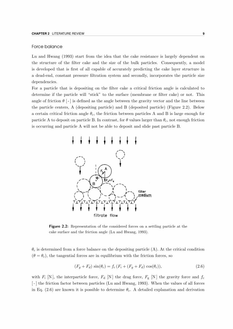
Force balance
Lu and Hwang (1993) start from the idea that the cake resistance is largely dependent on
the structure of the filter cake and the size of the bulk particles. Consequently, a model
is developed that is first of all capable of accurately predicting the cake layer structure in
a dead-end, constant pressure filtration system and secondly, incorporates the particle size
dependencies.
For a particle that is depositing on the filter cake a critical friction angle is calculated to
determine if the particle will “stick” to the surface (membrane or filter cake) or not. This
angle of friction θ [ - ] is defined as the angle between the gravity vector and the line between
the particle centers, A (depositing particle) and B (deposited particle) (Figure 2.2). Below
a certain critical friction angle θc, the friction between particles A and B is large enough for
particle A to deposit on particle B. In contrast, for θ values larger than θc, not enough friction
is occurring and particle A will not be able to deposit and slide past particle B.
Figure 2.2: Representation of the considered forces on a settling particle at the
cake surface and the friction angle (Lu and Hwang, 1993).
θc is determined from a force balance on the depositing particle (A). At the critical condition
(θ = θc), the tangential forces are in equilibrium with the friction forces, so
(Fg + Fd) sin(θc) = fc (Fi + (Fg + Fd) cos(θc)), (2.6)
with Fi [N ], the interparticle force, Fd [N ] the drag force, Fg [N ] the gravity force and fc
[ - ] the friction factor between particles (Lu and Hwang, 1993). When the values of all forces
in Eq. (2.6) are known it is possible to determine θc. A detailed explanation and derivation

10 2.2 MEMBRANE FOULING MODELS
of the different equations for the forces and parameters can be found in the original article
by Lu and Hwang (1993). The number of particles arriving at the cake surface is controlled
by the concentration and flux. The deposition point is determined by “dropping” particles
from a random position onto the cake or membrane and evaluating the angle of friction, as
explained above. Hence, a cake structure is obtained for a certain value of θc. For the particle
stacking, perfectly spherical particles are assumed but the porosity can be corrected with a
shape factor φs [ - ] for other shapes,
φs =1− ε
1− εsph, (2.7)
with ε [ - ] the actual porosity of the filter cake for non-sperical particles, εsph [ - ] the porosity
of the filter cake determined by the model, assuming perfect spheres. A full mathematical
description on the determination of φs is given in Cross et al. (1985).
Also the process of compression is considered, by calculating a porosity change based on a
fluid mass balance. The flux across the filter is calculated with the Kozeny-Carman equation,
J =∆p
l
ε3
νf K S2 (1− ε)2. (2.8)
This relation indicates that the flux J through a filter with depth l [m ] is influenced by the
TMP ∆p, the specific surface area S [m2 ], the kinematic viscosity of the fluid νf [m2 s−1 ],
the cake porosity ε and modulated by the Kozeny constant K [ - ].
An expression for the Kozeny constant in function of the porosity is obtained by solving the
Navier-Stokes equations and a continuity equation. Which in turn, when combined with Eq.
(2.8), gives rise to an equation for the specific filtration resistance α [m kg−1 ] of the filter
cake (Eq. 2.9).
α = K S2 1− εε3 ρs
, (2.9)
where ρs [kg m−3 ] is the density of the solids.
The predicted average porosity and average specific resistance of the filter cake closely ap-
proximate the experimental values. However, this model is restricted to dead-end filtration
which is rarely used in practice and this model is therefore not applicable to crossflow fil-
tration systems. For example, considering Eq. (2.6), one also needs to take into account the
lift force, history force, added mass force, etc. (Ghijs, 2014). The assumption of a spatially
homogeneous flux is also too straightforward and might influence the rate of local cake layer
build-up considerably, as well as the architecture and porosity. Nevertheless, the introduction
of a critical friction angle and the correction of the cake porosity with the shape factor of the
particles are valuable ideas.

CHAPTER 2 LITERATURE REVIEW 11
Pore blocking
A three-dimensional fouling model for the microfiltration of a polydisperse, charged solution
was developed by Yoon et al. (1999). An important improvement compared to Lu and Hwang
(1993) is the consideration of both pore blocking and cake layer formation. The model allows
for the simulation of flux in function of time for any concentration of iron oxide particles,
within the validated concentration range.
The effective particle deposition rate is calculated for each particle in the premised particle
size distribution (PSD), taking into account both processes that “push” the particle towards
the membrane and backtransport processes. This balance takes into consideration: inertia
lifting vl [m s−1 ] particle interaction vi [m s−1 ], convection v [m s−1 ], diffusion vd [m s−1 ] and
shear induced diffusion vs [m s−1 ]. The effective deposition velocity is the difference between
the backtransport velocity:
vtot(dp) = vd + vl + vs + vi , (2.10)
and the velocity toward the membrane v [m s−1 ], which is governed by the flux. With dp
[m ] the particle diameter. The gravitational settling velocity vg [m s−1 ] is not included
in this balance, so it is assumed that the effect of gravity is negligible. Subsequently, the
distribution of particle sizes that are able to deposit on the membrane, given the current flux
and backtransport velocity, is given by
Fnum(t, dp) = Fnum(t0, dp)(J(t)− vtot(dp))
J(t), (2.11)
with Fnum(t0, dp), the initial particle size distribution.
The cake layer is built up by depositing particles, sampled from Fnum(t, dp), one by one on the
membrane surface. The particle is dropped from a random location above the membrane. A
rolling algorithm is applied whenever a particle comes into contact with a previously settled
particle. The rolling continues until a stable position is reached, i.e. the particle touches three
already settled particles or the membrane surface. After deposition, the particle is tested for
pore blocking (Figure 2.3).

12 2.2 MEMBRANE FOULING MODELS
Unblocked Blocked
Membrane
Figure 2.3: Pore blocking rule implemented in the model of Yoon et al. (1999).
Only particles that touch the membrane surface and are centered within the pore
boundaries constitute to pore blocking. Figure adapted from Yoon et al. (1999).
The flux through the membrane is obtained with Darcy’s law in conjunction with a RIS
model, taking into account the inherent membrane resistance and pore blocking resistance
Rb [m−1 ]. The latter is computed from
Rb =N0
(N − 1)Rm, (2.12)
the flux follows from
J =∆pt,eff
νf (Rm +Rb). (2.13)
with N0 [ - ] the initial number of membrane pores, N [ - ] the free pores. Eq. (2.13) does
not contain a resistance term for the cake layer, but its effect is incorporated in ∆pt,eff [Pa ]
where the pressure drop over the membrane and cake is lowered by the pressure drop over
the cake ∆pc [Pa ]. The specific surface area and porosity vary with the cake layer depth.
Consequently, ε in the Kozeny-Carman equation (Eq. (2.8)) is not a constant. To deal with
this issue, the pressure drop is calculated over different “slices” in a recursive manner (Eq.
(2.14), Figure 2.4)
∆pT(i+ 1) = ∆pT(i)−νf ε
3i J
5S2i (1− εi)2
∆i, (2.14)
with Si [m2 ] the specific surface area of the particles and ∆i [m ] the thickness of a slice. It
is not clear why the Kozeny constant k is missing from Eq. (2.14).
After applying this scheme to every slice, ∆pc is obtained and the flux across the membrane
is computed with Eq. (2.13).

CHAPTER 2 LITERATURE REVIEW 13
Figure 2.4: Representation of the cake layer and the subdivision in different slices
Yoon et al. (1999).
Each time step, one particle is sedimented on the cake or membrane surface. The elapsed
time between two particle depositions is evaluated with Eq. 2.15.
∆t = ((J(t)− vtot(dp)) Am cb Fnum(t, dp)) (2.15)
with Am [m2 ] the specific membrane area. In the next time step, Eq. 2.11 is re-evaluated
with the new flux and a new particle is sampled from the new PSD.
The model performs quite well in the early stages of the filtration but the prediction accuracy
gradually declines with time. The simulated flux evolves to a steady state while experimental
values show that the flux keeps decreasing. The authors mention that unfulfilled assump-
tions for the backtransport equations as the probable cause, but the discrepancy between
the simulations and experimental data can also be due to the overestimation of the inertial
lift force. The channel inlet velocity is used as the velocity component in this force and this
component is overestimated considerably for particles in the slow moving fluid close to the
membrane surface. A more involved calculation of the velocity would probably enhance model
performance. The added value of this model lies in the introduction of pore blocking in a less
empirical manner, the polydispersity and charge interactions.
In the previously discussed models, the filter cake is either assumed spatially homogeneous,
with an average value for porosity and thickness, or heterogeneous along the depth. Yet,
heterogeneity along the longitudinal axis is never considered. This implies that there is no
spatial variation of the filtration resistance and flux. Consequently, these models are not able
to account for the spatial heterogeneity of membrane fouling. Li and Wang (2006) propose a
sectional approach to deal with this problem.
This sectional method allows the inclusion of turbulence, induced by aeration. The membrane
surface is subdivided into different sections with equal length in which the different variables
are tracked. The subdivision is along the longitudinal axis of the membrane, in contrast
to the method discussed in Yoon et al. (1999), where the “slices” are taken parallel to the
membrane.

14 2.2 MEMBRANE FOULING MODELS
For simulating the attachment of a sludge particle with a certain diameter (dp) on the mem-
brane surface, two forces are taken into account: the drag force Fd and the lift force Fl [N ].
The permeate flux drags the particles to the membrane and the lift force, a consequence of
the turbulent flow, is the opposing force. The balance between these two forces controls the
rate of particle deposition, expressed as a probability of deposition E [ - ]:
E =Fd
Fd + Fl(2.16)
For a probability E, the rate of biomass attachment becomes,
dM
dt= E C J (2.17)
with cb [kg m−3 ], the concentration of suspended solids (SS).
The effects of the continuous scouring through aeration is expressed as a rate of detachment
described by Eq. 2.18.
dM
dt= −KdMsf (2.18)
with Kd [s−1 ] the rate coefficient of sludge detachment and Msf [kg m−2 ] the mass of sludge
in the filter cake.
A Langmuir model is used for Kd, as it reaches a maximum for a very thick filter cake
and decreases with the cake thickness. The rate of detachment is essentially proportional
to the shear intensity, biomass stickiness and other properties of the sludge layer. The net
rate of sludge accumulation during a certain filtration period is obtained by solving the
abovementioned equations for biomass attachment and detachment. Li and Wang (2006) also
describe equations for the rate of sludge removal during the idle-cleaning period.
The filtration resistance is calculated using a RIS approach. The total resistance Rt is the
sum of the intrinsic membrane resistance, the resistance of the dynamic and stable cake
layer and the pore fouling resistance. All of these resistance terms involve an empirical
resistance parameter that needs calibration. Finally, Darcy’s law is used to calculate the flux
through the different membrane sections. As opposed to other models, sludge detachment is
considered and a sectional approach is established to capture the heterogeneity of membrane
fouling. However, this model involves a lot of parameters and the article does not provide
any information on the calibration.
Due to the many empirically described mechanisms, the performance of the model varies in
different operational conditions, which might just indicate that the model does not comprise
all relevant processes.
CHAPTER 2 LITERATURE REVIEW 15
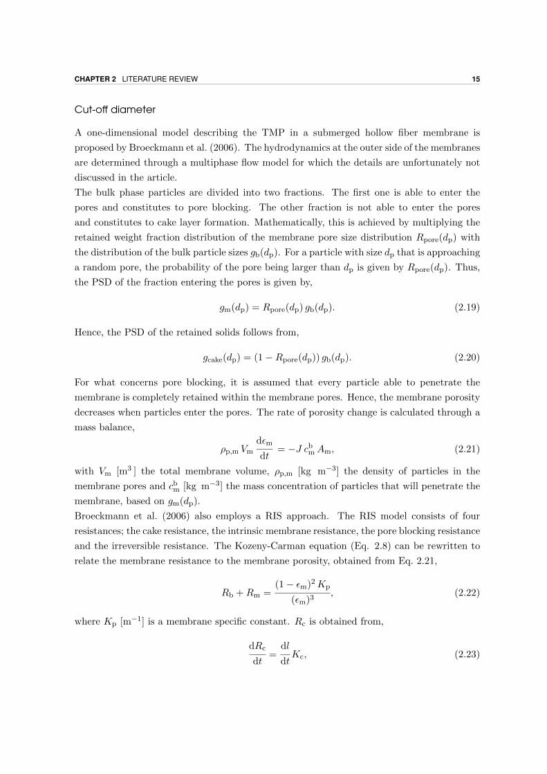
Cut-off diameter
A one-dimensional model describing the TMP in a submerged hollow fiber membrane is
proposed by Broeckmann et al. (2006). The hydrodynamics at the outer side of the membranes
are determined through a multiphase flow model for which the details are unfortunately not
discussed in the article.
The bulk phase particles are divided into two fractions. The first one is able to enter the
pores and constitutes to pore blocking. The other fraction is not able to enter the pores
and constitutes to cake layer formation. Mathematically, this is achieved by multiplying the
retained weight fraction distribution of the membrane pore size distribution Rpore(dp) with
the distribution of the bulk particle sizes gb(dp). For a particle with size dp that is approaching
a random pore, the probability of the pore being larger than dp is given by Rpore(dp). Thus,
the PSD of the fraction entering the pores is given by,
gm(dp) = Rpore(dp) gb(dp). (2.19)
Hence, the PSD of the retained solids follows from,
gcake(dp) = (1−Rpore(dp)) gb(dp). (2.20)
For what concerns pore blocking, it is assumed that every particle able to penetrate the
membrane is completely retained within the membrane pores. Hence, the membrane porosity
decreases when particles enter the pores. The rate of porosity change is calculated through a
mass balance,
ρp,m Vm
dεm
dt= −J cb
mAm, (2.21)
with Vm [m3 ] the total membrane volume, ρp,m [kg m−3] the density of particles in the
membrane pores and cbm [kg m−3] the mass concentration of particles that will penetrate the
membrane, based on gm(dp).
Broeckmann et al. (2006) also employs a RIS approach. The RIS model consists of four
resistances; the cake resistance, the intrinsic membrane resistance, the pore blocking resistance
and the irreversible resistance. The Kozeny-Carman equation (Eq. 2.8) can be rewritten to
relate the membrane resistance to the membrane porosity, obtained from Eq. 2.21,
Rb +Rm =(1− εm)2Kp
(εm)3, (2.22)
where Kp [m−1] is a membrane specific constant. Rc is obtained from,
dRc
dt=
dl
dtKc, (2.23)

16 2.2 MEMBRANE FOULING MODELS
with l [ m] the filter cake thickness and the specific cake resistance Kc,
Kc =k 90
dp2
(cc
ρs
)2
(1−
cc
ρs
)3, (2.24)
with cc [kg m−3 ] the mass concentration of the cake layer and dp [m ] the mean diameter of
bulk particles.
The cake layer formation is determined through a force balance (Figure 2.5).
Figure 2.5: Considered forces on a particle during filtration (Broeckmann et al.,
2006).
Ft [N ] is the tangential shear stress resulting from the liquid flow, Fτ [N ] is the friction force,
the normal force FN [N ] is the drag force resulting from the permeate flux and FA [N ] is
the adhesion force between the particles and the membrane. It is interesting to note that the
lift force is not included in this mass balance. All forces point towards the membrane, no
backtransport forces are considered to oppose this. With this fact in mind, a particle “sticks”
to the surface when the horizontal forces cancel out one another (Eq. 2.25) and
τW dp2 − µmax (FN + FA) = 0 , (2.25)
where τW [Pa ] is the shear stress and µmax [ - ] is the maximum friction coefficient.
From Eq. 2.25 an equation is derived for the maximum diameter of particles that are able
to adhere to the membrane surface, under the current filtration conditions. Particles larger
than this cut-off diameter will stay in the bulk phase.

CHAPTER 2 LITERATURE REVIEW 17
The growth of the cake layer is described by Eq. 2.26.
cc
dl
dt= J ω cb
c (2.26)
with ω [ - ] the bulk concentration of particles that are retained on the membrane surface,
i.e. the fraction of cbc [kg m−3 ] that is smaller than the cutoff diameter and cc the mass
concentration of the cake layer. Broeckmann et al. (2006) do not specify how cc is obtained
even though it is a crucial variable/parameter. Hence, it is assumed that cc is a parameter
that needs calibration.
During backflushing, particles are removed from the cake layer and pores. This process is
incorporated through simple, empirical models.
The strength of this model is the implementation of particle and pore size distributions as
typically only the former is included. Additionally, the implementation of backflushing pro-
cesses definitely improves the applicability of this model even though the formulation is simple
and empirical. The model however, has a few weaknesses including the lack of a sectional ap-
proach, many parameters and the low prediction accuracy when operational conditions differ
from calibration conditions. Furthermore, some assumptions that can be valid for hollow fiber
membrane systems might be invalid for other types of membrane filtration. The application
of the model on these systems is therefore less appealing. Both a strength and a weakness
of the model is its focus on constant flux filtration as most models address constant pressure
filtration instead.
Force balance, rolling and backwashing
Cao et al. (2015) elaborates a model to predict the TMP in an MBR that combines the
deposition criteria described in Broeckmann et al. (2006) and the particle depositing rules
from Yoon et al. (1999) in a RIS.
The cake layer is formed by particles that deposit one by one from a random location within
the boundaries of the simulated membrane surface. A particle drops until it reaches the
membrane surface or an already deposited particle; of the latter, a rolling algorithm is initiated
until a stable position is reached. Each series of particle depositions is defined as a “filtration
cycle”. Such a cycle ends when the total volume of deposited particles fulfills,
Vp,m =Am J tf pf cb
ρs, (2.27)
with tf [s ], the filtration time per filtration cycle and pf [ - ] the total fraction of depositable
particles. Eq. 2.27 is a combination of the equations presented in Yoon et al. (1999) and
Broeckmann et al. (2006).
The porosity of this newly formed cake layer is evaluated at the end of each filtration cycle
and is afterwards modified with a compression factor taking into account compression. With
18 2.2 MEMBRANE FOULING MODELS
both the porosity and cake thickness established it is possible to calculate the TMP using a
RIS. This model is furthermore extended with a backwashing model simulating cake removal
due to air scouring and backwashing sensu stricto.
The comprisal of different ideas and concepts results in a good performing model. It also
shows the importance of different factors such as PSD, compression and shear stress on
the characteristics of the filter cake. This model offers a porosity profile along the cake
thickness. Ideally this should be extended with a porosity profile along the cake length. Cake
compression is included albeit through a simple compression factor. The authors state the
need for a hydrodynamic model in order to provide a more realistic shear stress.
Biofouling
All of the abovementioned models describe particulate fouling. Nonetheless, it is important
to keep in mind that this is not the only fouling type, biofouling has a considerable impact
on different systems as this kind of fouling not solely occurs at membranes but also at heat
exchangers, pipes, feed spacers, etc. For this reason, a great deal of effort has been put in the
modelling of this fouling type. Consequently, these models are generally more advanced than
the RIS models mentioned above. Such a model is described in Picioreanu et al. (2009) and
Vrouwenvelder et al. (2010). This three-dimensional biofouling model simulates liquid flow,
mass transport of a soluble substrate and biofouling in the feed channels of reverse osmosis
and nanofiltration systems. The hydrodynamics are modelled via the steady-state Navier-
Stokes equations for incompressible laminar flow. The distribution of substrate in the system
is obtained through a mass balance. The biofilm is mimicked using an overlaying cellular
automaton including terms for growth, decay, convective and diffusive biomass spreading,
biomass attachment and detachment.
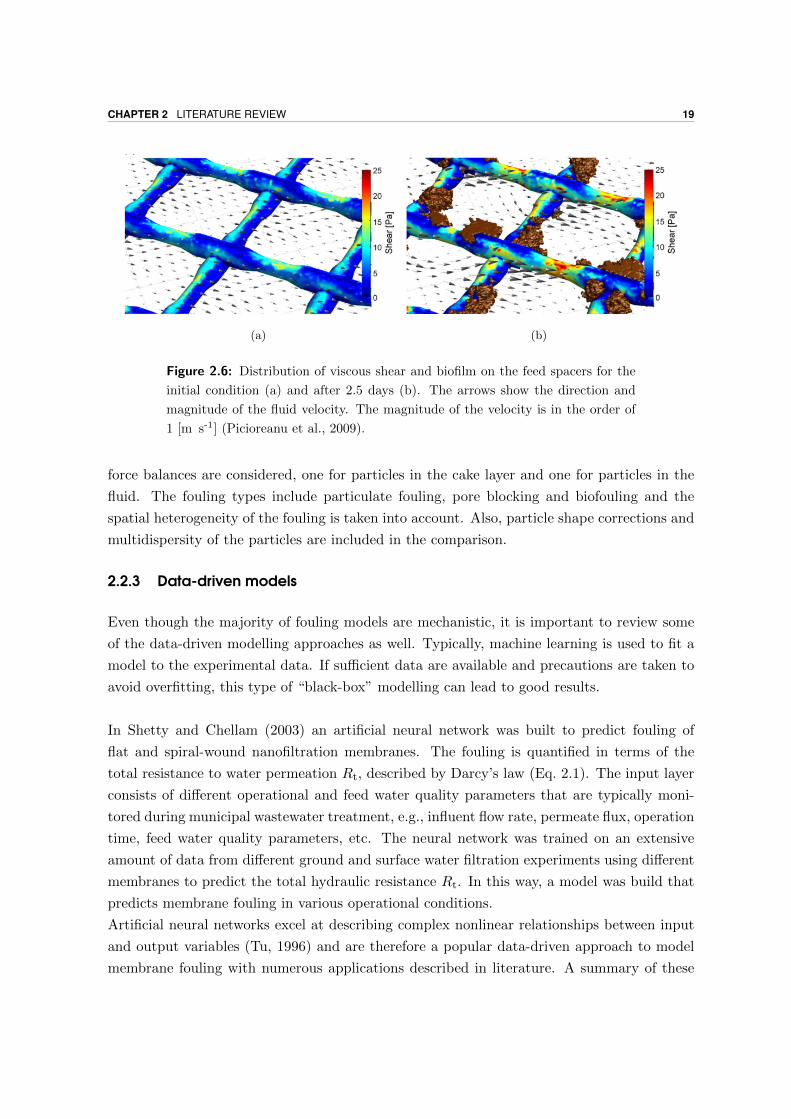
The simulations results (Figure 2.6) really show the importance of coupling the fouling model
with a fluid dynamics model. Figure 2.6 shows that when fouling persists, the fluid flow is
redirected and high shear channels form where no fouling occurs.
The authors show that the model is able to accurately predict feed channel pressure drop
and biomass accumulation on the feed spacers. The simulated, three-dimensional distribu-
tion profiles of biomass and velocity agree qualitatively with the experimental measurements.
The implementation of a fouling model in combination with computational fluid dynamics
(CFD) is a major improvement towards accurate, mechanistic models. This methodology,
implemented for biofouling is also highly relevant for particulate fouling as the fluid flow at
the membrane greatly affects cake formation and vice-versa. This approach should be carried
out in a sectional framework to incorporate heterogeneous cake formation.
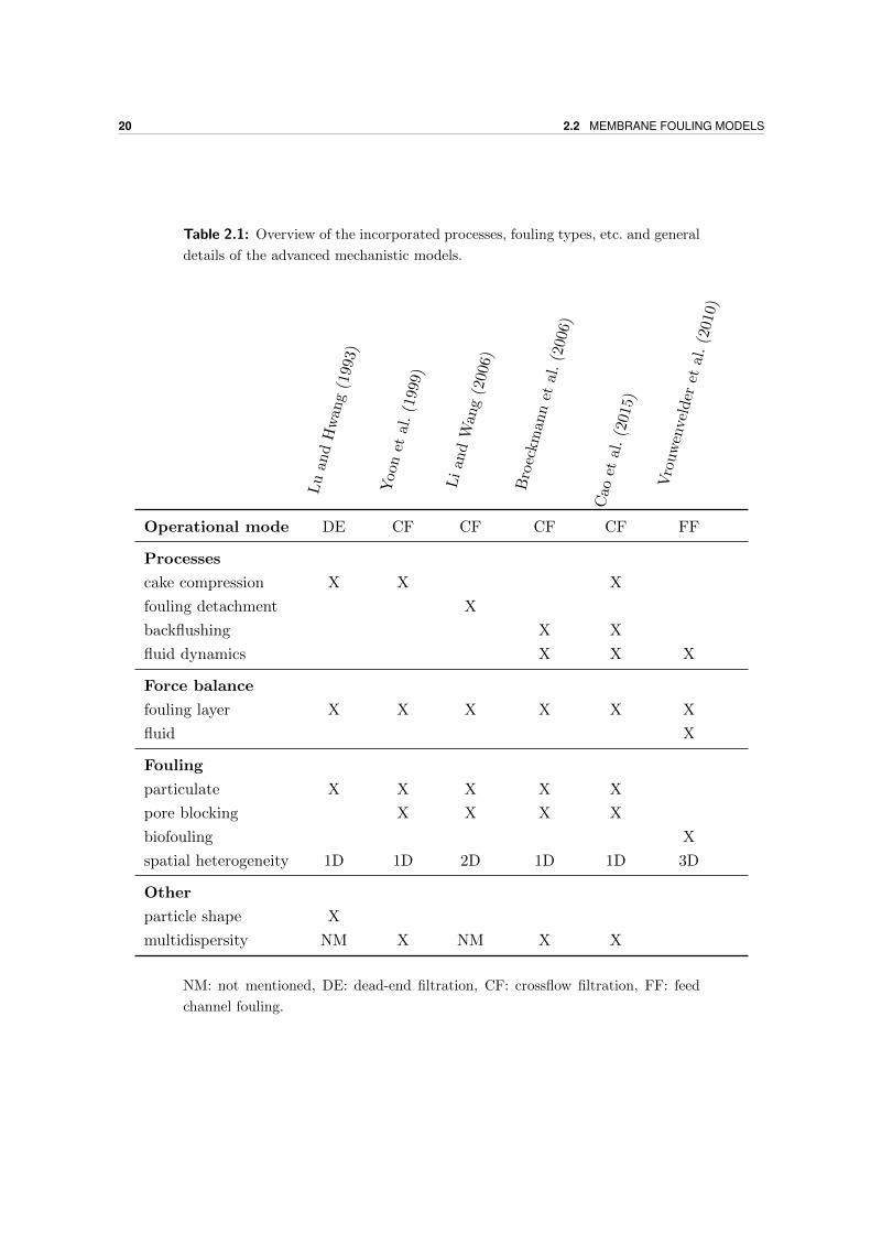
Table 2.1 provides an overview of the processes, fouling types, force balances, etc. that are
included in the abovementioned mechanistic models. The processes comprise cake compres-
sion, detachment of cake layer/biofilm, backflushing and dynamic fluid simulations. Two
CHAPTER 2 LITERATURE REVIEW 19
(a) (b)
Figure 2.6: Distribution of viscous shear and biofilm on the feed spacers for the
initial condition (a) and after 2.5 days (b). The arrows show the direction and
magnitude of the fluid velocity. The magnitude of the velocity is in the order of
1 [m s-1] (Picioreanu et al., 2009).
force balances are considered, one for particles in the cake layer and one for particles in the
fluid. The fouling types include particulate fouling, pore blocking and biofouling and the
spatial heterogeneity of the fouling is taken into account. Also, particle shape corrections and
multidispersity of the particles are included in the comparison.
2.2.3 Data-driven models
Even though the majority of fouling models are mechanistic, it is important to review some
of the data-driven modelling approaches as well. Typically, machine learning is used to fit a
model to the experimental data. If sufficient data are available and precautions are taken to
avoid overfitting, this type of “black-box” modelling can lead to good results.
In Shetty and Chellam (2003) an artificial neural network was built to predict fouling of
flat and spiral-wound nanofiltration membranes. The fouling is quantified in terms of the
total resistance to water permeation Rt, described by Darcy’s law (Eq. 2.1). The input layer
consists of different operational and feed water quality parameters that are typically moni-
tored during municipal wastewater treatment, e.g., influent flow rate, permeate flux, operation
time, feed water quality parameters, etc. The neural network was trained on an extensive
amount of data from different ground and surface water filtration experiments using different
membranes to predict the total hydraulic resistance Rt. In this way, a model was build that
predicts membrane fouling in various operational conditions.
Artificial neural networks excel at describing complex nonlinear relationships between input
and output variables (Tu, 1996) and are therefore a popular data-driven approach to model
membrane fouling with numerous applications described in literature. A summary of these
20 2.2 MEMBRANE FOULING MODELS
Table 2.1: Overview of the incorporated processes, fouling types, etc. and general
details of the advanced mechanistic models.
Lu
and
Hw
ang
(199
3)
Yoon
etal
.(1
999)
Li
and
Wan
g(2
006)
Bro
eckm
ann
etal
.(2
006)
Cao
etal
.(2
015)
Vro
uw
enve
lder
etal
.(2
010)
Operational mode DE CF CF CF CF FF
Processes
cake compression X X X
fouling detachment X
backflushing X X
fluid dynamics X X X
Force balance
fouling layer X X X X X X
fluid X
Fouling
particulate X X X X X
pore blocking X X X X
biofouling X
spatial heterogeneity 1D 1D 2D 1D 1D 3D
Other
particle shape X
multidispersity NM X NM X X
NM: not mentioned, DE: dead-end filtration, CF: crossflow filtration, FF: feed
channel fouling.

CHAPTER 2 LITERATURE REVIEW 21
studies can be found in Mirbagheri et al. (2015).
Dalmau et al. (2015) propose the use of model trees in predicting membrane fouling, which
combines linear regression with decision trees. Linear regression is a simple technique re-
sulting in a model with high bias but low variance, prone to underfitting nonlinear data. In
contrast, decision trees capture nonlinear patterns in the data, giving rise to models with low
bias and high variance, making it prone to overfitting (Dalmau et al., 2015). The combination
of both approaches leads to decision trees where each “leaf” is a linear model. The model tree
developed in the article consists of 35 multivariate linear equations. Each equation predicts
the TMP in various operating conditions. Model trees are capable of partially explaining the
system, unlike many other data driven methods (Dalmau et al., 2015).
Data-driven models can also be applied from a different point of view, that is membrane
state monitoring or fouling mechanism prediction. The former is elaborated by Maere et al.
(2012) and uses principal component analysis in combination with clustering to monitor the
fouling behaviour of MBR. A distinction is made between three different membrane states;
clean, reversibly fouled and irreversibly fouled, allowing for a real-time decision on possible
maintenance actions. A similar method is developed in Drews et al. (2009) where the domi-
nant fouling mechanism is identified by fitting different models to the data, each describing
different fouling mechanisms. The dominant fouling mechanism follows from the best fitting
model. Figure 2.7 presents the results of this approach.
Figure 2.7: Comparison between experimental and simulated flux/time curves
(Drews et al., 2009).

22 2.3 PROFILOMETRY
2.3 Profilometry
An important part of this thesis is the development of an experimental setup for the cal-
ibration and validation of the spatio-temporal model for filter cake formation. Membrane
filtration models are mostly calibrated and validated with data on the TMP and flux during
operation. However, considering that the main goal of this model is the characterisation of
filter cake formation mechanisms, it is meaningful to gather data about the filter cake prop-
erties for a goal-directed calibration/validation. This will be accomplished by a profilometric
characterisation of the filter cake.
Profilometry, surface metrology, surface topography, etc. are different terms used in liter-
ature to more or less describe the same process i. e. the three-dimensional characterisation of
a surface. The distinction between these terms lies in subtleties that are not relevant for this
study. These terms are therefore regarded as interchangeable.
Profilometric techniques can be classified in numerous categories, according to the charac-
teristics of the technique. In order to achieve a simple and straightforward classification,
a distinction is made between optical methods and non-optical methods. It is nonetheless
important to keep in mind that the main goal of this overview is to find a suitable technique
for the calibration/validation of the model and not a perfect classification of the profilometric
techniques.
2.3.1 Non-optical methods
The prominent method in this category is stylus profilometry (SP). In stylus profilometry,
the surface is characterised by the interaction of a sensing tip with the sample. The vertical
displacement of the tip is recorded while the stylus is moving across the sample’s surface
(Lonardo et al., 2002). Two main disadvantages of stylus profilometry can be identified (Stout
and Blunt, 2000; Lonardo et al., 2002). Firstly, this method is generally quite slow, taking
a long time to characterise a small area of the specimen. Secondly, the contact between the
instrument and sample can result in the deformation of the sample and an underestimation
of the height of soft surfaces. Consequently, stylus profilometry is not suitable for the surface
characterisation of a filter cake as it most certainly classifies as “soft”.
Atomic force microscopy (AFM) is generally not regarded as stylus profilometry because
there is no contact with the surface, since it is characterised via repulsive forces exterted on
the sensing tip. Nevertheless, the other working principles are quite similar. Atomic force
microscopy is mostly used for submicron measurements and its nanometer scale resolution
would be excessive for filter cake measurements, which are in the micrometer scale (White-
house, 1999).
CHAPTER 2 LITERATURE REVIEW 23
In scanning tunneling microscopy (STM) a metal tip scans the surface of the sample. A
voltage is applied over the gap between the tip and the specimen. When the conducting tip
is close to the surface, electrons will bridge the gap between the surface and the tip, resulting
in a current. Changes in surface height result in changes in magnitude of the current that are
subsequently recorded. STM is used for the surface characterisation on an atomic level and
is therefore not a suitable technique for this research (Binnig and Rohrer, 1982; Hansma and
Tersoff, 1987).
Scanning electron microscopy (SEM) utilises a beam of electrons to form a three-dimensional
image of the investigated surface. This beam is produced in an electron gunner or electron
emitter, accelerated by a set of anodes and focused on the specimen by a series of electromag-
nets. On collision, one part of the electrons will reflect of the surface, another part excites
the atoms of the specimen, thereby producing secondary electrons, and other electrons pen-
etrate the sample producing X-ray radiation. Both types of electrons and the X-rays can be
captured by specialised detectors giving rise to a profilometric image when the electron beam
is moved over the surface of the sample in a scanning motion (Reimer, 1985; Goldstein et al.,
2003).
2.3.2 Optical methods
The number of optical methods for the three-dimensional characterisation of a surface is vast.
It is impossible to discuss all these techniques, therefore a selection is made of the most dis-
tinct types in order to still give a comprehensive overview.
Interferometry is based on the interaction of multiple light beams and uses the superposi-
tion of waves to gather information about the surface characteristics (Hariharan, 2012). The
number of measurement techniques based on interferometry is enormous. However, the work-
ing principle of all these techniques is basically the same. A beam of light, is split by a glass
plate with a semi-reflective coating; one beam acts as a reference and is directly reflected
via a mirror to the detector while the second beam is reflected on the surface of the sample.
These two beams are recombined by the beamsplitter and will interfere. Figure 2.8 presents
a schematic overview of such a generic interferometer. Constructive interference is observed
when the path length is the same for both beams, giving rise to the interference signal with
the largest amplitude and hence the highest intensity. The signal intensity drops with bigger
path differences (the difference cannot exceed the wavelength). Consequently, an image is
obtained with different intensity values for each pixel. By altering the path length of one of
the beams it is possible to scan for other heights in the sample and a profilometric image
is formed. For these kind of measurements, white light is mostly used as it produces more
accurate results than monochromatic light.

24 2.3 PROFILOMETRY
White light interferometry (WLI) has a resolution limit of approximately 0.5µm due to diffrac-
tion effects (Conroy and Armstrong, 2005; Hariharan, 2012). Problems can arise from the
presence of thin films in the specimen that cause errors in the measurements (Conroy and
Armstrong, 2005). Hence, the presence of an aqueous layer in the filter cake poses a potential
risk for its profilometric characterisation.
Figure 2.8: The basic outline of an interferometer (Whitehouse, 1999).
Differential interference contrast microscopy (DICM) or Nomarski microscopy also adopts the
principles of interferometry, but both the reference and sample ray go through the sample
in two adjacent points. The difference in height of those points translates in a phase shift
between both rays. The rays are recombined and the resulting interference is proportional
to the difference in path length of the rays. A differential image is obtained of the surface
(Khalaf and Bainbridge, 1981).
Other interferometry related methods are digital holographic microscopy (DHM) (Kemper
et al., 2007) and optical coherence tomography (OCT) (Podoleanu, 2012). The working prin-
ciple of these techniques is very similar to DICM and will therefore not be elaborated.
Confocal laser scanning microscopy (CLSM) is basically a conventional light microscope with
the ability to illuminate a small section of the sample. The reflected light from the sample
is filtered through a pinhole that filters out all the out-of-focus light. Hence, it is possible to
illuminate a certain viewing depth, which is not possible with a conventional light microscope.
The combination of images from different depths gives rise to a three-dimensional structure
(Hocken et al., 2005). This method is technically not a profilometric technique as it actually
visualises the internal structures of a specimen. The maximal atainable resolution of confo-
cal laser scanning microscopy is about the same as that of a conventional light microscope
(Pawley, 1995). The use of CLSM as a tool for the profilometric characterisation of surfaces
is restricted by its low scanning rate and the problems that arise with the occurence of differ-
ent optical properties in one specimen (Cha et al., 2000). Pattern projection profilometry or
structured light profilometry establishes a three-dimensional profile by projecting light pat-
terns on the object and capturing the distortion of the pattern, from a different angle, with a
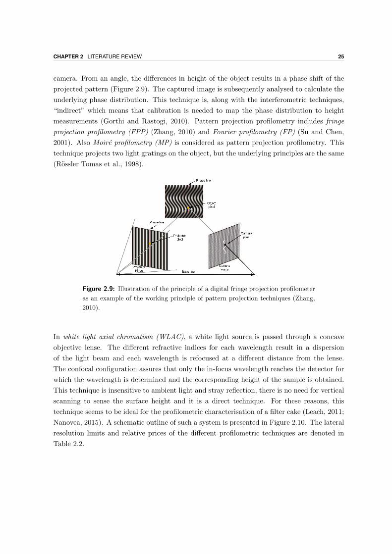
CHAPTER 2 LITERATURE REVIEW 25
camera. From an angle, the differences in height of the object results in a phase shift of the
projected pattern (Figure 2.9). The captured image is subsequently analysed to calculate the
underlying phase distribution. This technique is, along with the interferometric techniques,
“indirect” which means that calibration is needed to map the phase distribution to height
measurements (Gorthi and Rastogi, 2010). Pattern projection profilometry includes fringe
projection profilometry (FPP) (Zhang, 2010) and Fourier profilometry (FP) (Su and Chen,
2001). Also Moire profilometry (MP) is considered as pattern projection profilometry. This
technique projects two light gratings on the object, but the underlying principles are the same
(Rossler Tomas et al., 1998).
Figure 2.9: Illustration of the principle of a digital fringe projection profilometer
as an example of the working principle of pattern projection techniques (Zhang,
2010).
In white light axial chromatism (WLAC), a white light source is passed through a concave
objective lense. The different refractive indices for each wavelength result in a dispersion
of the light beam and each wavelength is refocused at a different distance from the lense.
The confocal configuration assures that only the in-focus wavelength reaches the detector for
which the wavelength is determined and the corresponding height of the sample is obtained.
This technique is insensitive to ambient light and stray reflection, there is no need for vertical
scanning to sense the surface height and it is a direct technique. For these reasons, this
technique seems to be ideal for the profilometric characterisation of a filter cake (Leach, 2011;
Nanovea, 2015). A schematic outline of such a system is presented in Figure 2.10. The lateral
resolution limits and relative prices of the different profilometric techniques are denoted in
Table 2.2.

26 2.3 PROFILOMETRY
Figure 2.10: Schematic representation of a white light axial chromatic confocal
profilometer (Nanovea, 2015).
Table 2.2: Overview of the lateral resolution and price class of the profilometric
thechniques. References: Song (1991) [1], Catto and Smith (1973) [2], Conroy
and Armstrong (2005) [3], Kemper et al. (2007) [4], Pawley (1995) [5], Nanovea
(2015) [6]
resolution price remarks
Non-optical
SP 0.5µm [1] $ dependent on the stylus size
AFM 0.1 nm [1] $$STM 0.1 nm [1] $$SEM 1 nm [2] $$$
Optical
Interferometry diffraction limited
WLI 0.5µm [3] $DICM 0.5µm $DHM 0.5µm $ good axial resolution (5 nm ) [4]
Focus detection
CLSM < 0.5µm [5] $$ close to diffraction limit
Pattern projection supermicron measurements
Other
WLAC 1µm [6] $
CHAPTER 3Spatio-temporal model of filter cake
formation
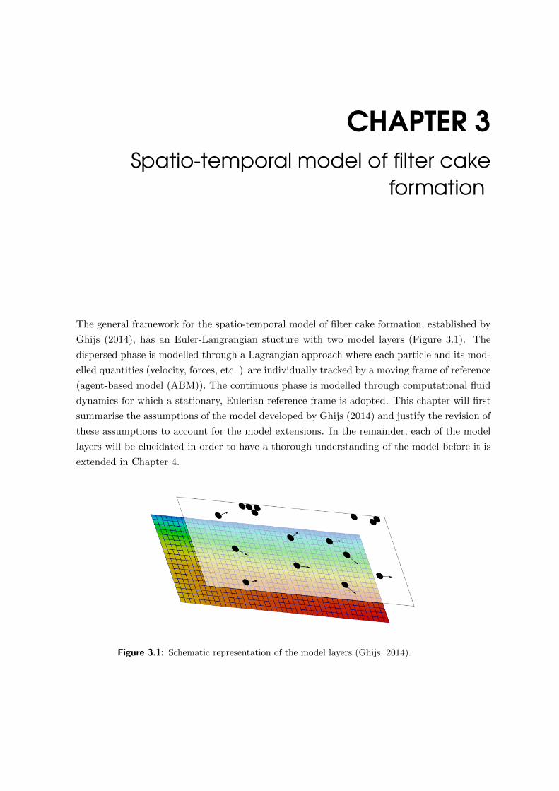
The general framework for the spatio-temporal model of filter cake formation, established by
Ghijs (2014), has an Euler-Langrangian stucture with two model layers (Figure 3.1). The
dispersed phase is modelled through a Lagrangian approach where each particle and its mod-
elled quantities (velocity, forces, etc. ) are individually tracked by a moving frame of reference
(agent-based model (ABM)). The continuous phase is modelled through computational fluid
dynamics for which a stationary, Eulerian reference frame is adopted. This chapter will first
summarise the assumptions of the model developed by Ghijs (2014) and justify the revision of
these assumptions to account for the model extensions. In the remainder, each of the model
layers will be elucidated in order to have a thorough understanding of the model before it is
extended in Chapter 4.
Figure 3.1: Schematic representation of the model layers (Ghijs, 2014).

28 3.1 ASSUMPTIONS
3.1 Assumptions
This study aims to develop a model that describes filter cake formation in MBRs as realisti-
cally as possible. It is nevertheless necessary to simplify certain processes in order to reduce
the computational demands and avoid the overcomplication of the model (Bender, 2000).
Therefore, assumptions were made in Ghijs (2014) about the nature of the particles and the
system in which they are modelled. Some of these assumptions are well-founded and will be
retained here, while others are revised and the model is extended with the necessary processes
to account for the extra complexity.
A first assumption is that all particles in the system are rigid and perfect spheres. This
originates from the force balance on the particles as some of these equations are derived
for rigid, perfect spheres in a flow field. This assumption might seem too simplistic, but
in a bottom-up modelling approach this is a good starting point. It is also assumed that
all particles are of the same size with diameter dp. For most of the filtration processes
the dispersed phase is made up of particles of different sizes and shapes and monodisperse
solutions are rare. Moreover, polydispersity has a significant impact on filter cake formation
and this assumption is therefore relaxed in this study. The corresponding model extension
involves a considerable programming effort as the implementation was strongly relying on the
assumption of monodispersity. This extension is discussed in Chapter 4.
There is no interaction of free moving particles in the bulk phase. Hence, there are no
collisions and free moving particles do not exert forces on each other. Coagulation of free
moving particles is consequently not considered. This assumption is justified, given the fact
that this model is constructed for laminar flows and the number of particle collisions in the
bulk fluid is limited.
The system is modelled in two dimensions, the forces and velocities describing the movement
of the particles in the bulk phase and the partial differential equations (PDEs) governing the
fluid behaviour are described in the x- and y-direction. In Ghijs (2014) it was assumed
that adding a third dimension would not impact the simulation results significantly so for
computational efficiency this dimension was left out. This assumption is also revised in this
study as simulation results in two dimensions showed an unrealistic “piling” of the particles
in the filter cake. The addition of a third dimension might resolve this issue and a system
modelled in three dimensions is more generic.
The flow profile of the fluid is only computed once at the beginning of the simulation.
This assumption implies a steady-state flow of the continuous phase throughout the entire
simulation, so that the formation of filter cake on the membrane surface has no effect on
the liquid flow profile. This “one-way” assumption is further discussed in Chapter 6 as it is
expected that the formation of filter cake greatly influences the liquid flow in close proximity
to the filter cake (Picioreanu et al., 2009). This, in turn, will have an impact on the filter cake
CHAPTER 3 SPATIO-TEMPORAL MODEL OF FILTER CAKE FORMATION 29
formation and for the accurate representation of this process, the model needs to be extended
with a bidirectional coupling between the two model layers.
Concerning filter cake formation as such, particles attach with a probability that is inversely
proportional to their absolute velocity (section 4.1.2) and attached particles cannot detach,
regardless of the shear stresses induced by the continuous movement of liquid over the filter
cake surface. This shortcoming is partially compensated by the abovementioned adhesion
probability. However, a complete force balance that supports detachment of particles from
the cake layer will lead to more realistic simulation results (Chapter 6).
The flux through the membrane is assumed to be constant in space and time. As
the formation of a filter cake layer on top of the membrane results in an increased filtration
resistance, the flux is expected to change locally according to the fouling intensity in constant
flux membrane filtration systems. The flux will be higher in “cleaner” regions and lower in
heavily fouled regions. Hence, it is necessary to extend the model to account for this, which
is discussed in Chapter 6.
3.2 Dispersed phase
The Lagrangian model of the dispersed phase consists of a system of differential equations that
describes a force balance of the free moving particles. The particle’s velocity is determined at
every time step and is expressed relatively with respect to the fluid velocity, i.e. Ur = Up−Uc,
with Up [m s−1 ] the relative velocity of the particle and Uc [m s−1 ] the local fluid velocity.
Newton’s second law is used to determine the particle velocity and follows from (Worner,
2003; Ghijs, 2014):
mp
d
dtUp(t) = ~Fsurf + ~Fbody, (3.1)
with mp [kg ] the particle mass. The force balance is divided in body forces ~Fbody [N ] that
are distributed over the entire volume of the particle and surface forces ~Fsurf [N ] that act on
the surface of the particles (Figure 3.2). For a particle immersed in a fluid, gravity ~Fg [N ] is
the only body force. The surface forces originate from (Worner, 2003; Ghijs, 2014):
• ~Farch [N ] the Archimedes force;
• ~Fp [N ] the force induced from the pressure gradient ∇ p;
• ~Fhydr [N ] the resulting hydrodynamic force, which consists of:
– ~Fdrag [N ] the drag force that minimises the difference between fluid velocity and
the particle velocity;
– ~Fam [N ] the added mass force that accelerates the fluid surrounding the particle;

30 3.2 DISPERSED PHASE
– ~Fhist [N ] the history force, which originates from the lagging fluid boundary layers
surrounding the accelerating particle;
– ~Flift [N ] the lift force, describing shear lift that is caused by the intertia effects in
the viscous flow around the particle.
Uc
UpUr
~Farch
~Fg
~Fhist
~Fdrag
~Fam
~Fp
~Flift
∇p
y
x
Figure 3.2: Schematic representation of the forces that act on free moving par-
ticles in a fluid, a negative Ur is assumed for the direction of the forces (Ghijs,
2014).
The total force balance on the particle can be written as:
~Ftot = ~Fg + ~Farch + ~Fp + ~Fdrag + ~Fam + ~Fhist + ~Flift . (3.2)
Now, the acceleration of the particles can be derived from Newton‘s second law (Eq. (3.1)).
However, this approach does not take into account the effects of stationary fluid boundaries
at the membrane surface. Faxen (1922) proposes the addition of a correction factor to include
these effects. Introducing the Faxen correction factor in Eq. (3.2) results in the Maxey-Riley
equation for the overall force balance on a particle submersed in a fluid (Maxey and Riley,
1983):
mpd
dtUp(t) = −3πηdp
(Ur −
1
24d2
p∇2Uc
)+ (mp − Vpρf) g
− 1
2Vpρf
(dUr
dt− 1
40d2
p
d
dt
(∇2Uc
))− Vp∇p−
3
2
√πηρfd
2p
∫ t
0
du(τ)/dτ√t− τ
dτ
− 1.615ρfd2p
(Ur −
1
24d2
p∇2Uc
)√µf |κ| sgn (κ) ,
(3.3)
CHAPTER 3 SPATIO-TEMPORAL MODEL OF FILTER CAKE FORMATION 31
with u = Ur − 124d
2p∇2Uc in the history term, Vp [m3 ] the particle volume and κ [s−1 ] the
fluid velocity gradient defined as,
κi =dUc,j
di(3.4)
where i and j represent directions in a two-dimensional Cartesian coordinate system.
3.3 Filter cake formation
By solving Eq. (3.3) one can accurately simulate the behaviour of the dispersed particles for
a given fluid flow profile. The first step in modelling the filter cake formation is the detection
of collisions of particles with the already formed cake layer or the membrane surface. This is
accomplished with a collision detection algorithm which is detailed in Chapter 4. To ensure
that not all collisions of the particles with the filter cake result in adhesion, this process is
governed by a probability. This function defines the probability P (Up) [ - ] for a particle to
attach to the filter cake in the event of a collision and is inversely proportional to the particle‘s
momentum:
P (Up) = e−kUp , (3.5)
with k [ - ] a parameter representing the “stickiness” of the particles which needs to be deter-
mined experimentally. Equation (3.5) is the only empirical equation and does not fit in the
model’s mechanistical mindset. Its role, however, is temporary and will become redundant
when a full force balance is in place for particles in the filter cake (chapter 6).
3.4 Continuous phase
This model layer describes the behaviour of the continuous phase as it flows continuously into
the filtration unit via the inlet and is discharged at the outlet and through the membrane
pores.
3.4.1 Fluid dynamics
The continuous phase is modelled through an Eulerian approach, the control volume is in-
cluded in a stationary reference frame and the flow quantities such as velocity and pressure
are described for each fixed point inside this control volume. The flow pattern and fluid
velocities of the continuous phase are obtained by solving the mass, momentum and energy
conservation equations, written as a set of PDEs. Depending on the fluid characteristics of
the modelled system, such as the rheology and flow regime (turbulent/laminar flow, single
phase/multiphase system), different sets of PDEs are used (Versteeg and Malalasekera, 1995;
Ranade, 2002).

32 3.4 CONTINUOUS PHASE
The first equation describes the conservation of mass within a given volume Ω [m3 ] and
is based on the following axiom: the rate of increase of mass in a fluid element is equal to the
net rate of flow into the fluid element since no mass can be created or destroyed, assuming
incompressibility. So,
∂ρf
∂t+∇(ρfUc) = 0, (3.6)
with Uc [m s−1 ] the fluid velocity in the volume Ω and ρf [kg m−3 ] the density. The com-
pressibility is negligible for most liquids and ρ can be assumed as constant. Consequently, for
incompressible fluids (Versteeg and Malalasekera, 1995):
∂ρf
∂t= 0, (3.7)
and
∇(ρfUc) = ρf∇Uc, (3.8)
so that
∇Uc = 0. (3.9)
The conservation of momentum, as a second equation, is governed by a force balance acting
on Ω. By taking into consideration the body forces such as gravity and the surfaces forces
such as the compressive force and friction force and inserting them into Newton’s second law
of motion, one obtains:
ρf
(δUc
δt+ Uc ·∇Uc
)= −∇p+∇ · τ + f, (3.10)
with τ [N ] the viscous stress tensor and f [N m−1 ] the external body forces. In most of the
cases, f only consists of the gravitational force (Versteeg and Malalasekera, 1995; Ranade,
2002).
For an incompressible, Newtonian fluid the viscous stresses are proportional to the rates
of deformation and constant viscosity can be assumed. Consequently, the stress tensor τ
in Eq. (3.10) can be written in terms of the viscosity µf and fluid velocity, leading to the
Navier-Stokes equation for incompressible flow (Versteeg and Malalasekera, 1995),
ρf
(δUc
δt+ Uc ·∇Uc
)= −∇p+ µf ∇2Uc + f . (3.11)
For this study, an isothermal flow is considered and the equations for the conservation of
energy are not relevant and are therefore not discussed. The set of PDEs (3.9) and (3.11) is
called the Navier-Stokes system for incompressible flow (Versteeg and Malalasekera, 1995).

CHAPTER 3 SPATIO-TEMPORAL MODEL OF FILTER CAKE FORMATION 33
3.4.2 Computational fluid dynamics
The Navier-Stokes equations provide an accurate theoretical basis for modelling dynamic
fluid behaviour. However, these equations are complex, non-linear and coupled, making the
solution quite complex and in practice more often than not, analytical solutions are non-
existent. It is therefore necessary to use numerical methods in order to obtain a solution for
the modelling problem at hand, which is the scientific domain of CFD (Ranade, 2002).
“Computational fluid dynamics is a set of numerical methods applied to obtain
approximate solutions of problems of fluid dynamics and heat transfer.”
— (Zikanov, 2010)
Depending on the characteristics of the fluid in the system, different fluid dynamics equations
need to be used. The Navier-Stokes equations (3.9) and (3.11) are derived for a Newtonian,
incompressible fluid in an isothermal system which is a good representation for modelling
wastewater and other liquids used in membrane filtration systems.
After selecting the appropriate flow equations and boundary conditions, the equations are
discretised either using finite volume methods (FVMs) or finite element methods (FEMs).
The FEM is not used in this work and is therefore not elucidated.
In the FVM, the domain is subdivided into a finite number of cells with a certain volume,
where the values of the different variables are integrated values of their respective cells, stored
in the center points of the cells. The discretised PDEs are obtained by constructing the
conservative form for which volume integrals are used for the conservative components and
surface integrals of the divergence terms (Ranade, 2002; Patankar, 1980). For a scalar property
φ, the discretised transport equations can be written as follows:
∫ t+∆t
t
∫V
δ(ρ φ)
δtdV +
∫S
ρU φ ·ndS =
∫S
Γ∇φ ·ndS +
∫V
Sφ dV
dt , (3.12)
with Γ the diffusion coefficient and Qφ the source of φ. The first term in Eq. (3.12) denotes
a temporal derivative and is zero for the steady-state solution. The second term describes
the convective flux of φ through the control volume. The third and fourth term, respectively,
represent diffusion and the volumetric sources and sinks of φ that cannot go under the first
three terms. A solution for the flow problem can be obtained by applying Eq. (3.12) to every
cell in the discretised spatial domain, and utilising a numerical solving method (Ranade,
2002).


CHAPTER 4Model development
The profound study of other membrane fouling modelling approaches described in literature
(Chapter 2) and the critical analyses of the assumptions and model framework proposed
by Ghijs (2014) (Chapter 3) identified the processes that require further development and
those that are not yet incorporated. The proposed model extensions include changes in the
model framework, sensu strictu, and the development of accessory tools such as a graphical
user interface (GUI) for the analysis of the simulation results and post-processing. This
chapter discusses the implemented model extensions and tools in-depth and is concluded by
an overview of the model’s architecture.
4.1 Polydispersity
Broeckmann et al. (2006) demonstrate the influence of particle and membrane pore size
distributions on cake layer formation and pore blocking. Meng et al. (2006) also identify the
PSD as an important factor that affects membrane fouling. Moreover, it is generally known
that a heterogeneous mixture of particle sizes gives rise to a closer packing of particles in
the filter cake, which has an important impact on the filtration resistance. It is expected
that a dense filter cake is more resilient towards liquid shear stresses and thus less prone to
detachment.
It is clear that characterising the feed flow of filtration processes as a homogeneous and
monodisperse suspension of perfect spheres is not realistic. The strong depency of the filter
cake architecture and characteristics on the particles size demonstrates the importance of
a more accurate representation of the dispersed phase. Extending the model towards poly-
dispersity of the bulk phase is therefore a crucial step in establishing a realistic membrane
fouling model. The extension of the model towards polydispersity is somewhat complicated
as many processes described by the model, e.g. the attachment of particles, are dependent
on the particle diameter and the model implementation often relies on the assumption of
36 4.1 POLYDISPERSITY
monodispersity. Hence, this modification required the revision and adaptation of some pro-
cess implementations.
The flocculation of free moving particles in the bulk phase is not considered by this model.
Although, the inclusion of polydispersity makes it possible to account for particle aggregates
by representing sludge flocs as one particle with a bigger diameter. It is also possible to model
non-spherical particles as a multidisperse aggregate of spheres (Hubbard, 1996).
4.1.1 Particle sampling
For a monodisperse stream of particles entering the membrane filter, the number of particles
entering each time step N [ - ] is given by,
N = 6Ucf cbA
ρs π dp3
∆t , (4.1)
with Ucf [m s−1 ] the crossflow velocity at the inlet, A [m2 ] the inlet surface area and ∆t [s ]
the elapsed time per time step.
When modelling a multidisperse bulk phase, Eq. (4.1) does not hold as dp is not constant. In
order to have a quantitative measure of incoming particles, this flow is expressed as a mass
flow rate,
dm
dt= Ucf cbA , (4.2)
with m [kg ] the mass of incoming particles. Multiplying Eq. (4.2) with the total simulation
time ttot [s ] results in an estimated value of the total mass inflow during the entire simulation,
mtot = Ucf cbA ttot. (4.3)
The next step is the development of a sampling procedure to represent the multidisperse feed
flow, characterised by a PSD. Particles are sampled from this PSD until the total mass, as
determined by Eq. (4.3), is attained.
A PSD depicts the relative amount of particles present in the bulk phase as a function of the
particle size, based on volume or number. Experimentally determined PSDs are based on a
finite number of measurements, making dp a discrete variable for which the inverse cumulative
distribution function (CDF) sampling algorithm is the most efficient pseudo-random number
generator, given a cumulative PSD. This sampling procedure randomly generates a number
in the interval [0,1] and searches in the given PSD for the diameter value that corresponds to
the probability value that is the closest to the generated number. It can be proven that for
a large number of samples, this procedure results in the original PSD.
Lastly, the number of particles that enters each time step is simulated stochastically. For

CHAPTER 4 MODEL DEVELOPMENT 37
a sufficiently small time step ∆t, the average number of particles entering each step (Eq.
(4.1)) is smaller than one. As it is not possible to introduce a non-integer number of parti-
cles, the latter represents the probability of a particle entering on a certain time step, this
procedure is depicted in Algorithm 1.
Algorithm 1: Stochastic implementation of the number of particles entering the system.
Calculate average number of incoming particles per time step;
for i = 1 to number of time steps do
if random number [0,1] < number of particles per time step then1 particle enters system;
elseNo particles enter system;
end
end
When considering the introduction of a dispersion into a tubular system with a fully developed
parabolic flow, the particles should not be equally distributed across the inlet, since they
would then accumulate in the regions with low velocities close to the boundaries and diminish
in the middle regions with high velocities, creating a parabolic concentration profile. This
phenomenon is shown in Figure 4.1 (b). In order to prevent such an unrealistic behavior, the
inlet positions of the particles are determined by a sampling procedure so that the introduction
of particles at a certain position is corrected for the local variation in the fluid velocity. This
is accomplished by first normalising the parabolic velocity profile at the inlet so that it
sums up to one, yielding a proper probability mass function (PMF). The PMF is integrated
and the resulting CDF can be used in the above-mentioned inverse CDF sampling procedure.
However, this inverse CDF sampling procedure can be computationally demanding for discrete
distributions with a lot of bins. The latter is relatively low for the PSD but for the velocity
profile this number is too high, resulting in an inefficient sampling procedure which slows
down the model considerably. Hence, a power law (f(x) = a xb) is fitted to the CDF and
the inverse CDF is determined analytically (Figure 4.2). This approach gives rise to a faster
sampling procedure than its discrete counterpart. Figure 4.1 shows the simulation of particles
entering a fully developed parabolic flow with and without the parabolic sampling procedure.
38 4.1 POLYDISPERSITY
(a) (b)
Figure 4.1: Simulated flow of particles close to the wall of a tube with a diameter
of 8 mm. The incoming particles are sampled with (a) and without the velocity
correction (b).
Figure 4.2: Comparison of the fitted power law (f(x) = a xb) and the discrete
CDF.
4.1.2 Filter cake formation
Another consequence of a variable particle diameter is the necessity to modify the collision
detection algorithm, registering collisions of particles with the membrane or the filter cake.
In Ghijs (2014), the filter cake is implemented in a discrete manner such that the filter cake
thickness is tracked at a predefined longitudinal resolution. However, as the filter cake is built
up out of spherical particles, the surface is highly irregular and curvy. In order to accurately
represent this surface in a discrete way, the discretisation step should be at least one order
of magnitude lower than the smallest particle diameter. Hence, storing filter cake thicknesses
explicitely is only computationally efficient when considering a thick cake layer. Furthermore,
for the evaluation of certain filter cake characteristics such as porosity, segregation and the
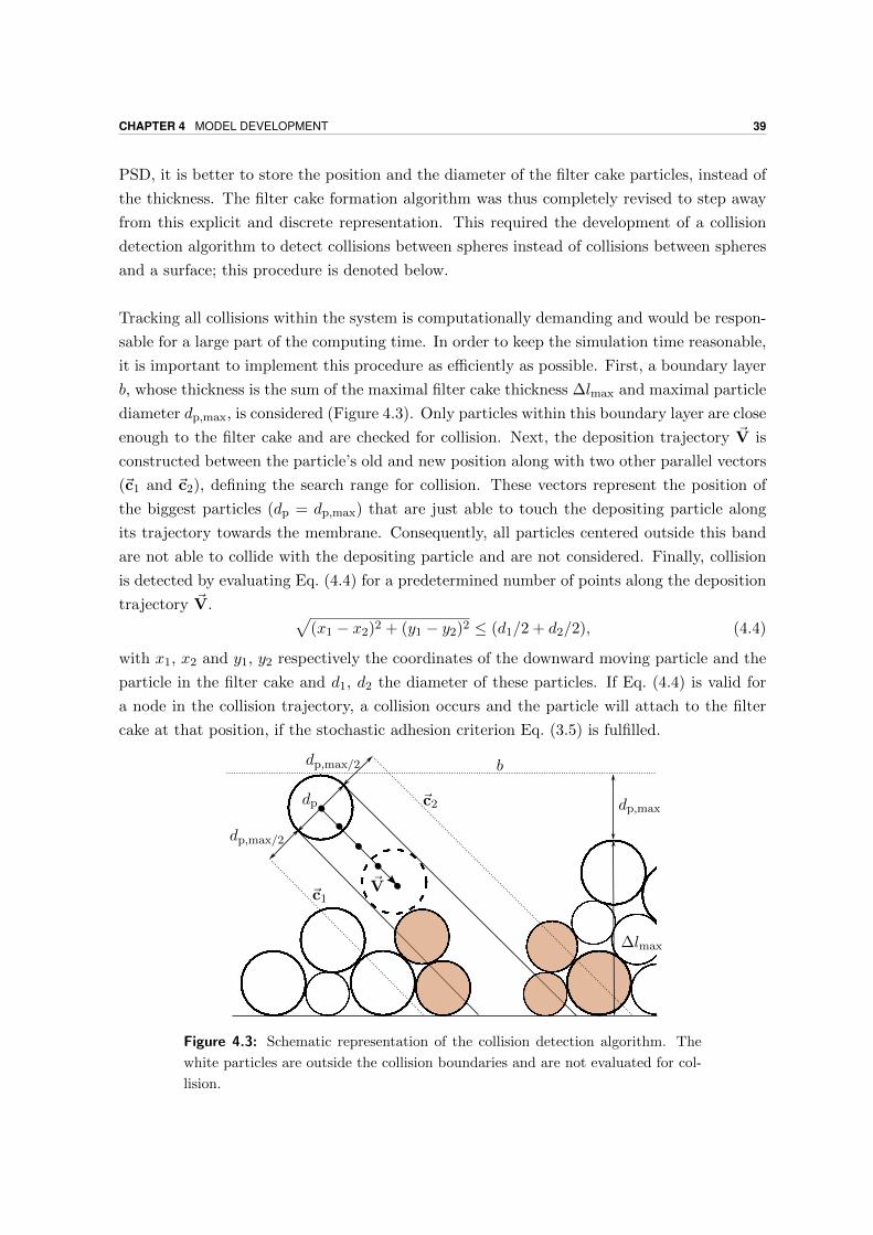
CHAPTER 4 MODEL DEVELOPMENT 39
PSD, it is better to store the position and the diameter of the filter cake particles, instead of
the thickness. The filter cake formation algorithm was thus completely revised to step away
from this explicit and discrete representation. This required the development of a collision
detection algorithm to detect collisions between spheres instead of collisions between spheres
and a surface; this procedure is denoted below.
Tracking all collisions within the system is computationally demanding and would be respon-
sable for a large part of the computing time. In order to keep the simulation time reasonable,
it is important to implement this procedure as efficiently as possible. First, a boundary layer
b, whose thickness is the sum of the maximal filter cake thickness ∆lmax and maximal particle
diameter dp,max, is considered (Figure 4.3). Only particles within this boundary layer are close
enough to the filter cake and are checked for collision. Next, the deposition trajectory ~V is
constructed between the particle’s old and new position along with two other parallel vectors
(~c1 and ~c2), defining the search range for collision. These vectors represent the position of
the biggest particles (dp = dp,max) that are just able to touch the depositing particle along
its trajectory towards the membrane. Consequently, all particles centered outside this band
are not able to collide with the depositing particle and are not considered. Finally, collision
is detected by evaluating Eq. (4.4) for a predetermined number of points along the deposition
trajectory ~V. √(x1 − x2)2 + (y1 − y2)2 ≤ (d1/2 + d2/2), (4.4)
with x1, x2 and y1, y2 respectively the coordinates of the downward moving particle and the
particle in the filter cake and d1, d2 the diameter of these particles. If Eq. (4.4) is valid for
a node in the collision trajectory, a collision occurs and the particle will attach to the filter
cake at that position, if the stochastic adhesion criterion Eq. (3.5) is fulfilled.
dp
dp,max/2
dp,max/2
~V
∆lmax
dp,max
b
~c1
~c2
Figure 4.3: Schematic representation of the collision detection algorithm. The
white particles are outside the collision boundaries and are not evaluated for col-
lision.

40 4.2 EXTENSION TO A THREE-DIMENSIONAL MODEL
To summarise, the new collision detection algorithm is more accurate due to the continuous
and implicit representation of the filter cake and its performance is improved by constraining
the detection of collisions to a boundary layer and limiting the search for possible collisions
in a narrow zone spanning the collision search band.
4.2 Extension to a three-dimensional model
The model extension from two dimensions to three dimensions is a logical step towards a
realistic filter cake representation. Yet it leads to a considerable increase in the number
of modelled particles and one may wonder whether the added value of process knowledge
outweighs the extra computational burden. There are, however, two key reasons to chose for
a three-dimensional model.
In Ghijs (2014), the simulations suffered from an unrealistic “piling” of particles in the filter
cake. Even with the possibility of an elastic collision, it was observed that most particles are
caught by previously formed filter cake patches. Due to the lack of a third dimension, a piece
of filter cake will catch all incoming particles and keep growing as there is no mechanism
that counteracts this. It is hypothesised that by extending the model to three dimensions,
a single piece of filter cake will have less impact on the further development of the fouling.
Nonetheless, the increased dimensionality will most likely not entirely solve this issue; to do
so, the model should be extended with a rolling algorithm. Such an algorithm is described in
Cao et al. (2015) and simulates the three-dimensional rolling of spheres. To include this in
the model, a transition to three dimensions is imperative.
As can be expected, the flow of particles in a three-dimensional flow field is similar to that in a
two-dimensional flow field. Still, it is necessary to modify some of the implemented processes.
First, the force balance (Eq. (3.3)) is extended with a third direction (z). The resulting force
in this direction is not influenced by ~Fg and ~Farch and can be written in terms of ~Fp, ~Fdrag,~Fam, ~Fhist and ~Flift.
Secondly, the lift force in the x- and y-direction has to be extended with an additional gradient
in the z-direction. In two dimensions, the inertial lift force has one component in both the
x-direction and y-direction (Saffman, 1965):
~Flift,x = −1.615 ρf d2p Ur,x
√√√√µf
∣∣∣∣∣dUr,xdy
∣∣∣∣∣ sign
(dUr,x
dy
), (4.5)
~Flift,y = −1.615 ρf d2p Ur,y
√√√√µf
∣∣∣∣∣dUr,ydx
∣∣∣∣∣ sign
(dUr,y
dx
), (4.6)
with Ur,x and Ur,y the relative particle velocity in the x- and y-direction respectively .

CHAPTER 4 MODEL DEVELOPMENT 41
In three dimensions, Eqs. (4.5) and (4.6) need to be extended with a gradient in the z-
direction. The x-component of the lift force, for example, should now be written as:
~Flift,x = −1.615 ρf d2p Ur,x
√√√√µf
∣∣∣∣∣dUr,xdy
∣∣∣∣∣ sign
(dUr,x
dy
)
+
√√√√µf
∣∣∣∣∣dUr,xdz
∣∣∣∣∣ sign
(dUr,x
dz
) .(4.7)
With the correct force balance established, the model is now capable of describing the parti-
cle’s motion in a three-dimensional flow field.
The adaptation of the filter cake formation process for three dimensions is straightforward.
More precisely, the collision trajectory vector is described in three dimensions and the colli-
sion search boundaries are now represented by a cylinder. In spite of these changes, the main
working principle remains the same.
4.3 Parallelisation
As mentioned in Section 4.2, the extension to three dimensions comes at a higher computa-
tional expense. For a 10 kg m−3 dispersion of 50µm particles (ρp = 1000 kg m−3) flowing in a
two-dimensional tube (10 cm × 10 mm), approximately 8× 10⁸ particles have to be processed
each second of simulated time, excluding the particles in the filter cake. When considering a
box with the same dimensions and a width of 5 mm, this number increases to 8× 10¹⁰, which
indicates the difficulty of maintaining a reasonable simulation time to computational time
ratio (SCR). For one processor, the SCR is in the order of 1 × 10⁻⁴. The implementation
of the filter cake formation, sampling procedures and force balance are already very efficient,
leaving little room for optimisation. Hence, the best solution is to parallelise the implemen-
tation to enable simultaneous computation on multiple processors (cores). This is done by
assigning every processor a part of the spatial domain, so that it performs the calculations
for the particles present in that part. Every predefined number of time steps, information
is exchanged between the cores and the particles that moved to a neighbouring part of the
spatial domain are reallocated to the appropriate cores. In this way, a good SCR (∼ 1×10⁻³)
is obtained without the need of convoluted code optimisation.
4.4 Model architecture
The overall model architecture is depicted in Figure 4.4. The model takes three inputs,

42 4.4 MODEL ARCHITECTURE
Parallelisation Merge processors
Geometry
Meshing
CFD
Sampling
PSD
Main loop
Initialisation
Calculation loop
Simulation
Parameters
Checking
stability
Adding
particles
Calculating
positions
Filter cake
formation
Filter cake
structure
Figure 4.4: Overview of the model architecture. The MBR geometry, PSD and
the general simulation parameters are the inputs of the model. The output of the
model is the filter cake structure, represented by the (x, y, z)-coordinates and
diameter of the particles in the cake.
CHAPTER 4 MODEL DEVELOPMENT 43
the first being the MBR geometry. This geometry is defined in a Python script and con-
verted to a suitable mesh by SALOME’s Python interpreter. Then, this mesh is exported
to OpenFOAM and the solution for the pressure and velocity fields are obtained using the
simpleFOAM solver. These fields are subsequently imported to MATLAB. The second input
is the PSD of the particle diameters in the feed flow. During the initialisation, the total mass
of particles that will flow through the system during the simulation is estimated and sampled
as discussed in Section 4.1.1. The last input is a list of general simulation parameters, such as
the concentration of particles cb, the stickiness parameter k, the time window considered by
the history force, etc. Based on these values, it is first checked if the calculation of the Stokes
drag force is stable (Ghijs, 2014). If so, the main loop is entered. If not, an appropriate time
step is suggested that leads to stable simulations.
In the main loop, the computational domain is partitioned and assigned to a number of
processors (Section 4.3). Each processor caries out a calculation loop to simulate the dispersed
phase. Each time step, new particles are added to the system, the new positions of all particles
are determined and the filter cake formation is simulated. After a fixed number of time steps,
the information of the processors is collected and the domain is repartitioned. This procedure
is repeated until the predefined simulation time is reached.
4.5 Software
4.5.1 MATLAB
MATLAB (v2015a, MathWorks), an abbreviation for matrix laboratory, is a high level matrix-
based scripting language licensed by MathWorks. This commercial software package has an
extensive library of readily available functions, mostly for engineering and scientific appli-
cations (MathWorks, 2016). MATLAB plays a central role in this master thesis, it is the
backbone of the model linking all the different processes, software and files and acts as a basis
for the GUI.
4.5.2 Python
Python (v2.7.3, Python Software Foundation) is an open source, high-level programming
language that is more general-purpose than MATLAB. Python is licensed by the Python
Software Foundation and comes with a vast number of modules, both from the standard
library and community-contributed libraries, making it widely applicable (Python-Software-
Foundation, 2016). For this master thesis, Python is mainly used as scripting language for
the automated generation of meshes through SALOME’s Python interpreter.
44 4.6 POST-PROCESSING USER INTERFACE
4.5.3 SALOME
SALOME (v7.6.0, OPEN CASCADE) is an open source software for the pre- and post-
processing of numerical simulations. It is used as a pre-processor for the generation of the
geometry and mesh before using CFD. SALOME provides an application programming inter-
face (API) for Python that enables scripting of the geometry and mesh, providing a generic
workflow for the creation of variable geometries and meshes. SALOME is licensed by OPEN
CASCADE (Open-Cascade, 2016).
4.5.4 OpenFOAM
OpenFOAM (v2.2.2, OpenFOAM foundation) (Open Source Field Operation and Manipula-
tion) is an open source software package that provides a vast number of solvers and utilities
for the calculation of continuum mechanics (OpenFOAM-Foundation, 2016). OpenFOAM is
written in C++ and has no GUI, all manipulations are done by changing files and running
applications from the command line. Two solvers are used for this master thesis, the simple-
FOAM solver is a steady-state solver for turbulent and laminar flow and the pimpleFOAM
solver is a large time-step transient solver for turbulent flow.
4.6 Post-processing user interface
This advanced mechanistic membrane fouling model aims at identifying the key mechanisms
of membrane fouling in filtration processes. In addition to the accurate modelling of mem-
brane fouling, it is important that the simulation results are analysed critically. Therefore,
a GUI was developed as post-processing tool that enables, amongst other things, a detailed
visualisation of the filter cake and force balance (Figure 4.5). The prominent utilities of this
GUI are elaborated below.
By clicking the “Play” button [1] the in silico filtration experiment is displayed in real-
time speed. With the “Track” button [2], one can track individual particles throughout the
simulation, while useful information about the particle’s velocity, acceleration, size, etc. is
displayed at [2a]. While tracking a particle, the force balance for the two main directions
(x,y) is shown in two top right plots [2b]. This information is very useful for determining
the main driving forces of filter cake formation under various operational conditions. The
button “Detail” [3] visualises the filter cake at a user-defined position in the form of a two-
dimensional projection. The user is able to “scroll” through the filter cake along the length
of the membrane for a visual inspection. A three-dimensional visualisation of the filter cake
can be requested by clicking “3D” [4]. Diameter coloring [5] assigns a different color to each
particle size which can be convenient for the visualisation of certain phenomena, such as
particle size segregation in the cake layer due to preferential sedimentation (Section 5.2.3).

CHAPTER 4 MODEL DEVELOPMENT 45
The PSDs of the feed flow, filter cake, dispersed phase and the entire system (control) can
be visualised by checking of “PSD” [6]. Finally, by clicking “Save” [7] all the information of
the detailed filter cake is stored in a MATLAB workspace variable for further manipulation
outside the GUI.
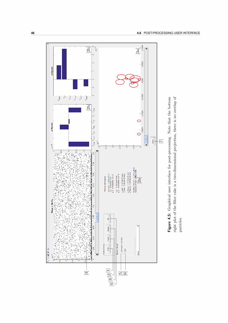
46 4.6 POST-PROCESSING USER INTERFACE
[1]
[2]
[3]
[4]
[5]
[6]
[7]
[2a]
[3a]
[3]
[2b
][2
b]
Fig
ure
4.5
:G
rap
hic
alu
ser
inte
rface
for
post
-pro
cess
ing.
Note
that
the
bott
om
righ
tp
lot
ofth
efi
lter
cake
isa
two-d
imen
sion
al
pro
ject
ion
,th
ere
isn
oov
erla
pof
par
ticl
es.
CHAPTER 5Results and discussion
One sometimes finds what one is not looking for.
— Sir Alexander Fleming
This chapter presents the results of this work and is structured in two major sections. In
the first section (5.1), the model-based design of a laboratory scale microfiltration unit is
discussed. This unit will be used to collect data for the calibration and validation of the
model, and it is of utmost importance that a structured flow is achieved near the membrane. In
Section 5.2, a scenario analysis is performed to assess the movement of particles and the filter
cake formation under different operational conditions. First, a description of the modelled
system and the assumptions are discussed and the benchmark operational parameters are
disclosed. Next, a qualitative validation of the bulk phase force balance is performed in order
to assess the accuracy of the predicted movement. In the end, the spatial segregation of the
particles and the effect of polydispersity is investigated.
5.1 Calibration and validation: model-based design of a filtrationunit
In order to determine the value of the adhesion parameter k, which can be interpreted as the
stickiness of the filter cake, a calibration has to be performed. Furthermore, as the objective
of this research is the characterisation of filter cake formation, it is important to assess the
model’s accuracy through validation. Both calibration and validation require the acquisition
of experimental data. For that reason, a laboratory scale, crossflow microfiltration unit was
designed. Such an experimental setup enables full control of the operational conditions and
measured quantities during filtration. Moreover, in addition to tracking typical filtration
variables such as the transmembrane pressure and flux, it is possible to use profilometric
techniques for the acquisition of specific filter cake properties such as the cake thickness, sur-
face roughness and other, more advanced features for a goal-directed calibration/validation.
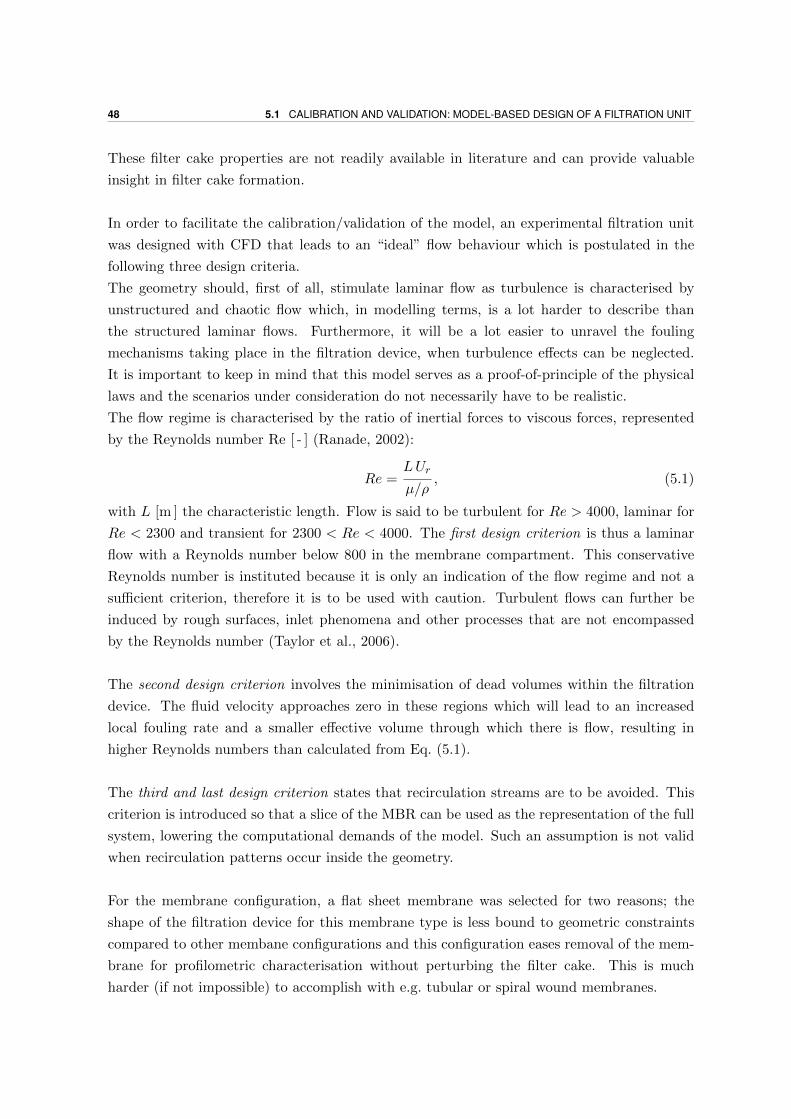
48 5.1 CALIBRATION AND VALIDATION: MODEL-BASED DESIGN OF A FILTRATION UNIT
These filter cake properties are not readily available in literature and can provide valuable
insight in filter cake formation.
In order to facilitate the calibration/validation of the model, an experimental filtration unit
was designed with CFD that leads to an “ideal” flow behaviour which is postulated in the
following three design criteria.
The geometry should, first of all, stimulate laminar flow as turbulence is characterised by
unstructured and chaotic flow which, in modelling terms, is a lot harder to describe than
the structured laminar flows. Furthermore, it will be a lot easier to unravel the fouling
mechanisms taking place in the filtration device, when turbulence effects can be neglected.
It is important to keep in mind that this model serves as a proof-of-principle of the physical
laws and the scenarios under consideration do not necessarily have to be realistic.
The flow regime is characterised by the ratio of inertial forces to viscous forces, represented
by the Reynolds number Re [ - ] (Ranade, 2002):
Re =LUr
µ/ρ, (5.1)
with L [m ] the characteristic length. Flow is said to be turbulent for Re > 4000, laminar for
Re < 2300 and transient for 2300 < Re < 4000. The first design criterion is thus a laminar
flow with a Reynolds number below 800 in the membrane compartment. This conservative
Reynolds number is instituted because it is only an indication of the flow regime and not a
sufficient criterion, therefore it is to be used with caution. Turbulent flows can further be
induced by rough surfaces, inlet phenomena and other processes that are not encompassed
by the Reynolds number (Taylor et al., 2006).
The second design criterion involves the minimisation of dead volumes within the filtration
device. The fluid velocity approaches zero in these regions which will lead to an increased
local fouling rate and a smaller effective volume through which there is flow, resulting in
higher Reynolds numbers than calculated from Eq. (5.1).
The third and last design criterion states that recirculation streams are to be avoided. This
criterion is introduced so that a slice of the MBR can be used as the representation of the full
system, lowering the computational demands of the model. Such an assumption is not valid
when recirculation patterns occur inside the geometry.
For the membrane configuration, a flat sheet membrane was selected for two reasons; the
shape of the filtration device for this membrane type is less bound to geometric constraints
compared to other membane configurations and this configuration eases removal of the mem-
brane for profilometric characterisation without perturbing the filter cake. This is much
harder (if not impossible) to accomplish with e.g. tubular or spiral wound membranes.
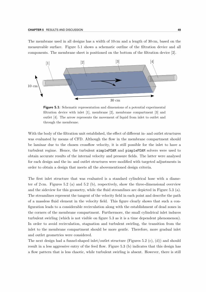
CHAPTER 5 RESULTS AND DISCUSSION 49
The membrane used in all designs has a width of 10 cm and a length of 30 cm, based on the
measureable surface. Figure 5.1 shows a schematic outline of the filtration device and all
components. The membrane sheet is positioned on the bottom of the filtration device [2].
10 cm
30 cm
[1] [3][2] [4]
Figure 5.1: Schematic representation and dimensions of a potential experimental
filtration device with inlet [1], membrane [2], membrane compartment [3] and
outlet [4]. The arrow represents the movement of liquid from inlet to outlet and
through the membrane.
With the body of the filtration unit established, the effect of different in- and outlet structures
was evaluated by means of CFD. Although the flow in the membrane compartment should
be laminar due to the chosen crossflow velocity, it is still possible for the inlet to have a
turbulent regime. Hence, the turbulent simpleFOAM and pimpleFOAM solvers were used to
obtain accurate results of the internal velocity and pressure fields. The latter were analysed
for each design and the in- and outlet structures were modified with targeted adjustments in
order to obtain a design that meets all the abovementioned design criteria.
The first inlet structure that was evaluated is a standard cylindrical hose with a diame-
ter of 2 cm. Figures 5.2 (a) and 5.2 (b), respectively, show the three-dimensional overview
and the sideview for this geometry, while the fluid streamlines are depicted in Figure 5.3 (a).
The streamlines represent the tangent of the velocity field in each point and describe the path
of a massless fluid element in the velocity field. This figure clearly shows that such a con-
figuration leads to a considerable recirculation along with the establishment of dead zones in
the corners of the membrane compartment. Furthermore, the small cylindrical inlet induces
turbulent swirling (which is not visible on figure 5.3 as it is a time dependent phenomenon).
In order to avoid recirculation, stagnation and turbulent swirling, the transition from the
inlet to the membrane compartment should be more gentle. Therefore, more gradual inlet
and outlet geometries were considered.
The next design had a funnel-shaped inlet/outlet structure (Figures 5.2 (c), (d)) and should
result in a less aggressive entry of the feed flow. Figure 5.3 (b) indicates that this design has
a flow pattern that is less chaotic, while turbulent swirling is absent. However, there is still

50 5.1 CALIBRATION AND VALIDATION: MODEL-BASED DESIGN OF A FILTRATION UNIT
(a) (b)
(c) (d)
(e) (f)
(g) (h)
(i) (j)
Figure 5.2: Tested laboratory scale filtration device geometries with CFD: three-
dimensional geometry (left), sideview (right)
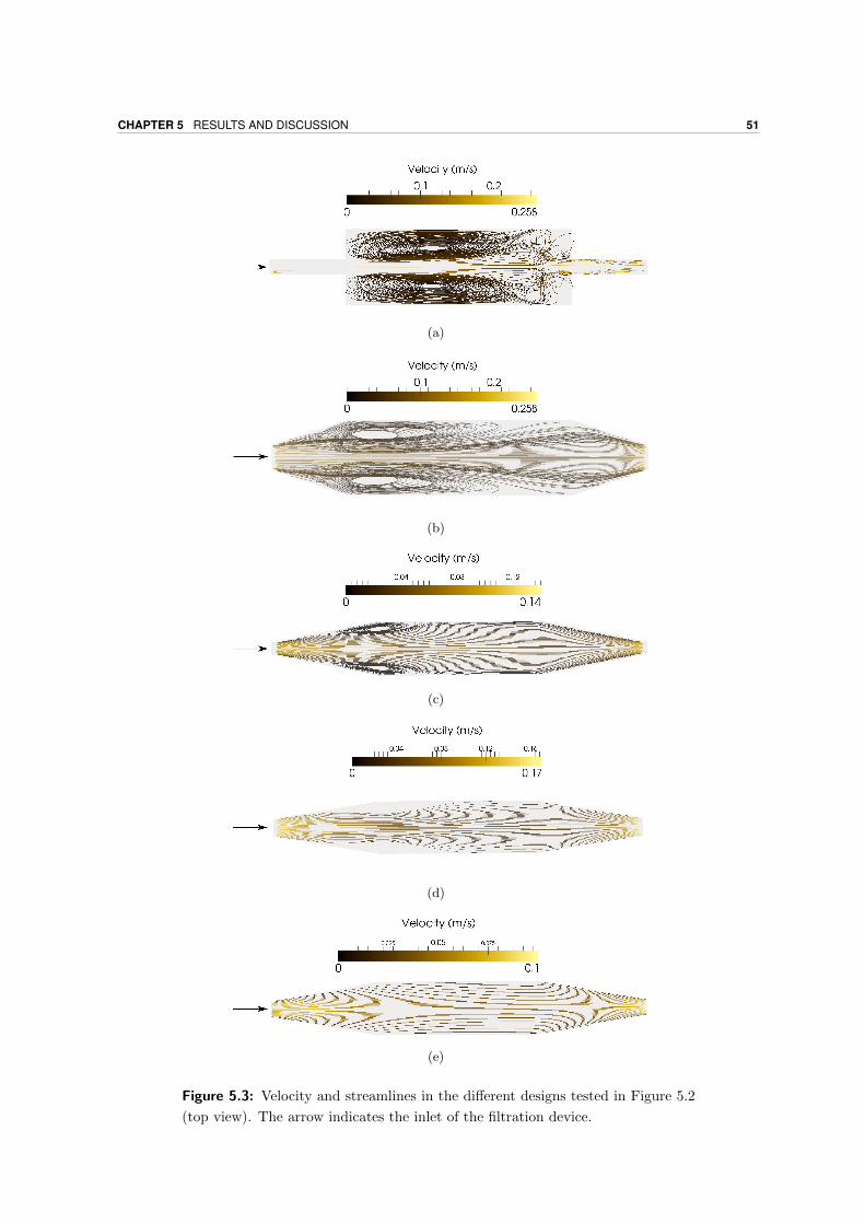
CHAPTER 5 RESULTS AND DISCUSSION 51
(a)
(b)
(c)
(d)
(e)
Figure 5.3: Velocity and streamlines in the different designs tested in Figure 5.2
(top view). The arrow indicates the inlet of the filtration device.

52 5.2 CASE STUDIES
a considerable recirculation of the fluid and presence of dead volumes. Hence, the feed flow
still disturbs the overall fluid dynamics too much.
In an attempt to get rid of the recirculation, the inlet length was doubled from 10 to 20 cm
(Figures 5.2 (e), (f)). Figure 5.3 (c) shows the streamlines for this configuration. Although
there is a substantial improvement, it still does not meet the requirements set by the design
criteria. By using an inlet with a rectangular cross section rather than a square, it is possible
to obtain a flow profile without recirculation (Figures 5.2 (g), (h) and Figure 5.3 (d)), but
these changes introduce two stagnant regions at the entrance of the membrane compartment.
Finally, a suitable design was obtained by introducing a bigger inlet and reducing the height
of the membrane compartment so to obtain a flat configuration (Figures 5.2 (i), (j)). This
configuration also has the advantage of being a lot easier to manufacture. Since this geometry
generates a flow profile that fulfills all design criteria (Figure 5.3 (e)), it will be constructed
and used for the experimental measurements. The technical drawings for this design are given
in Appendix A.
5.2 Filtration model: case studies
5.2.1 Setup
In order to investigate the impact of the model extensions and to verify if the filter cake
build-up occurs in a realistic way, a tubular membrane was chosen as subject of a scenario
analysis. This geometry has the advantage of being symmetrical, it gives rise to a parabolic
flow profile and enables the possibility of simulating a long length. Therefore, the tubular
geometry was selected instead of the optimal geometry according to the results reported in
Section 5.1. The tubular membrane had an inner diameter of 8 mm and a length of 60 cm.
The feed was introduced at the channel inlet and a constant flux was instituted through
the porous wall (membrane). A crossflow velocity and flux of respectively 0.04 m s−1 and
36 LMH (1 × 10⁻⁵ m s−1 ) were chosen as benchmark values. The PSD of the feed flow was
experimentally determined with a particle size analyser (DIPA 2000) on a sample of MBR
sludge from municipal wastewater (Figure 5.4) and the number average diameter, 40.82µm,
was used as benchmark particle size for monodisperse simulations. Ghijs (2014) demonstrated
that high values of k result in a slow filter cake formation while low values induce an increased
piling of the particles. Therefore, k = 2 results in a good trade-off between the rate of
filter cake formation and the roughness of the cake. The other benchmark parameters are
summarised in Table 5.1.
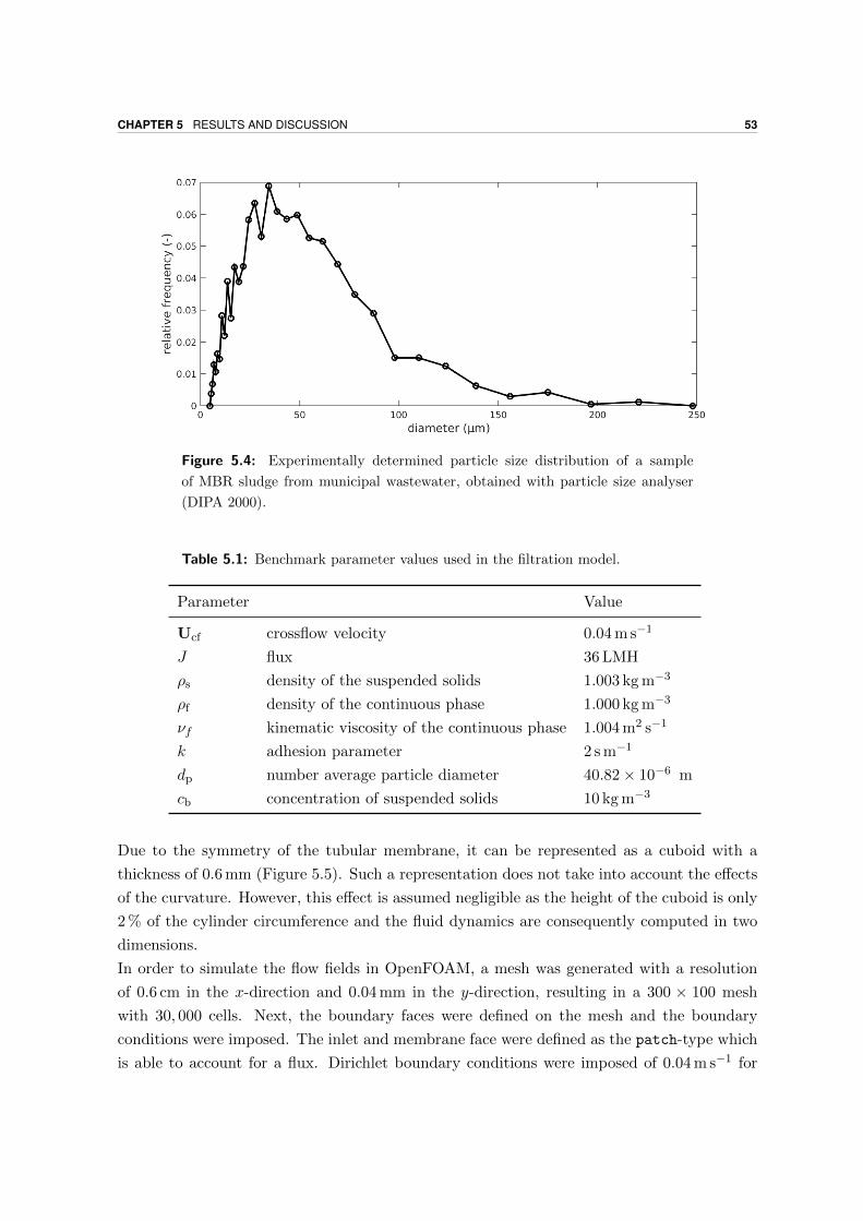
CHAPTER 5 RESULTS AND DISCUSSION 53
Figure 5.4: Experimentally determined particle size distribution of a sample
of MBR sludge from municipal wastewater, obtained with particle size analyser
(DIPA 2000).
Table 5.1: Benchmark parameter values used in the filtration model.
Parameter Value
Ucf crossflow velocity 0.04 m s−1
J flux 36 LMH
ρs density of the suspended solids 1.003 kg m−3
ρf density of the continuous phase 1.000 kg m−3
νf kinematic viscosity of the continuous phase 1.004 m2 s−1
k adhesion parameter 2 s m−1
dp number average particle diameter 40.82× 10⁻⁶ m
cb concentration of suspended solids 10 kg m−3
Due to the symmetry of the tubular membrane, it can be represented as a cuboid with a
thickness of 0.6 mm (Figure 5.5). Such a representation does not take into account the effects
of the curvature. However, this effect is assumed negligible as the height of the cuboid is only
2 % of the cylinder circumference and the fluid dynamics are consequently computed in two
dimensions.
In order to simulate the flow fields in OpenFOAM, a mesh was generated with a resolution
of 0.6 cm in the x-direction and 0.04 mm in the y-direction, resulting in a 300 × 100 mesh
with 30, 000 cells. Next, the boundary faces were defined on the mesh and the boundary
conditions were imposed. The inlet and membrane face were defined as the patch-type which
is able to account for a flux. Dirichlet boundary conditions were imposed of 0.04 m s−1 for

54 5.2 CASE STUDIES
the x-velocity at the inlet, 1× 10⁻⁵ m s−1 for the y-velocity at the membrane and 0 m s−1 for
all other directions, assuming zero slip at the walls. For the pressure, Neumann zero gradient
boundary conditions were set at the inlet, membrane, and symmetry plane. The outlet was
also defined as the patch-type with a zero gradient Neumann boundary condition for the
velocity and a Dirichlet boundary condition of atmospheric pressure, assuming free outflow.
The inside face was defined as a symmetryPlane-boundary implying a periodic boundary
condition for the velocity, while the front and back faces are set to empty to indicate a two
dimensions simulation. The Reynolds number for these conditions is 320, which is well within
the laminar region.
The steady-state solution for this flow problem was obtained via the simpleFoam solver which
is primarly used for turbulent, incompressible Newtonian flow but is also valid under laminar
conditions.
4 mm0.6 mm 60 cm
[1] [3]
[5]
[4]
[2]
xy
z
Figure 5.5: Three-dimensional representation of the modelled system, boundary
faces and their respective fluxes, denoted by the arrows. The boundary faces
consist of inlet [1], outlet [2], membrane [3], inside [4], front and back [5].
The steady-state solution for the relative kinematic pressure ψ [m2 s−2 ], x-velocity and y-
velocity is displayed in Figure 5.6. The absolute pressure shows a linear decrease from
101, 371 Pa to atmospheric pressure, 101, 325 Pa. Concerning the fluid velocity, a transition
from the uniform profile at the inlet to a parabolic profile is observed. Due to the zero-slip
boundary condition at the membrane, the fluid is moving slower near the walls and the incom-
ing fluid is forced towards the middle section. After this transition, the x-velocity exhibits a
fully developed parabolic flow and the y-velocity remains quasi constant at −1× 10⁻⁵ m s−1.
In order to facilitate the interpretation of the results, all simulations performed in the remain-
der of this chapter are based on the fully developed middle section of the tubular membrane
(30 cm). The involvement of inlet phenomena will only complicate the interpretation and are
removed from the equation. Lastly, it is important to note that all simulations employ the
benchmark parameter values as given in Table 5.1, unless indicated otherwise.
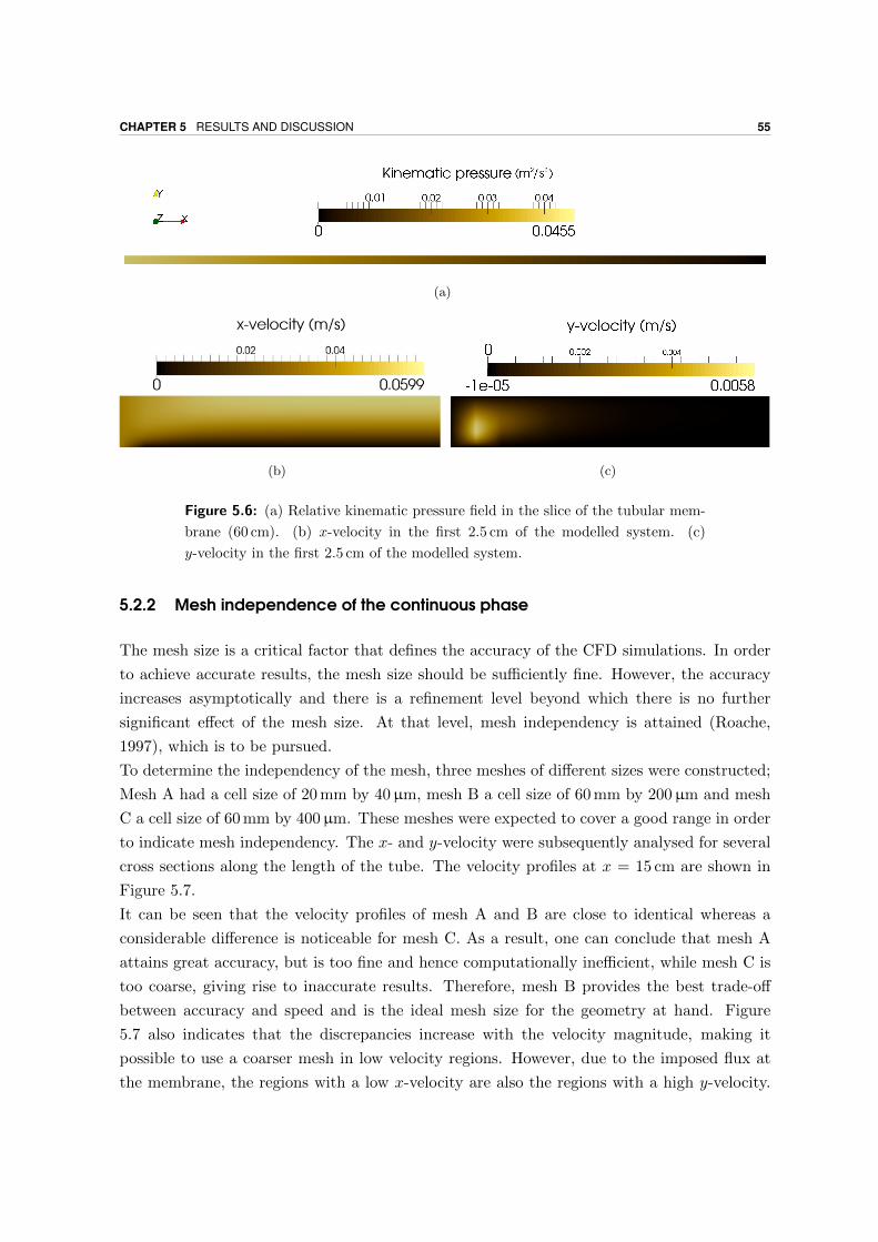
CHAPTER 5 RESULTS AND DISCUSSION 55
(a)
(b) (c)
Figure 5.6: (a) Relative kinematic pressure field in the slice of the tubular mem-
brane (60 cm). (b) x-velocity in the first 2.5 cm of the modelled system. (c)
y-velocity in the first 2.5 cm of the modelled system.
5.2.2 Mesh independence of the continuous phase
The mesh size is a critical factor that defines the accuracy of the CFD simulations. In order
to achieve accurate results, the mesh size should be sufficiently fine. However, the accuracy
increases asymptotically and there is a refinement level beyond which there is no further
significant effect of the mesh size. At that level, mesh independency is attained (Roache,
1997), which is to be pursued.
To determine the independency of the mesh, three meshes of different sizes were constructed;
Mesh A had a cell size of 20 mm by 40µm, mesh B a cell size of 60 mm by 200µm and mesh
C a cell size of 60 mm by 400µm. These meshes were expected to cover a good range in order
to indicate mesh independency. The x- and y-velocity were subsequently analysed for several
cross sections along the length of the tube. The velocity profiles at x = 15 cm are shown in
Figure 5.7.
It can be seen that the velocity profiles of mesh A and B are close to identical whereas a
considerable difference is noticeable for mesh C. As a result, one can conclude that mesh A
attains great accuracy, but is too fine and hence computationally inefficient, while mesh C is
too coarse, giving rise to inaccurate results. Therefore, mesh B provides the best trade-off
between accuracy and speed and is the ideal mesh size for the geometry at hand. Figure
5.7 also indicates that the discrepancies increase with the velocity magnitude, making it
possible to use a coarser mesh in low velocity regions. However, due to the imposed flux at
the membrane, the regions with a low x-velocity are also the regions with a high y-velocity.

56 5.2 CASE STUDIES
Hence, a non-uniform mesh should be a fine mesh near the membrane, a coarser mesh in the
middle and finer mesh at the center of the tube. Due to the simple geometry and the fast
convergence for mesh B, this non-uniform meshing strategy is considered as too complex for
a minor efficiency gain, and was therefore not implemented.
(a)
(b)
Figure 5.7: Velocity profile of the velocities in x-direction (a) and y-direction (b)
at x = 15 cm from the inlet for three meshgrids. Mesh A with a cell size of 20 mm
by 40µm, mesh B with a cell size of 60 mm by 200µm and mesh C with a cell size
of 60 mm by 400µm.

CHAPTER 5 RESULTS AND DISCUSSION 57
5.2.3 The Segre-Silberberg effect: a qualitative validation
Rigid spheres flowing in tubular channels under laminar conditions are subjected to a ra-
dial migration due to shear gradient and inertia-induced lift forces. This effect is called the
Segre-Silberberg effect and was experimentally observed by Segre and Silberberg (1961). Fol-
lowing the work of Segre and Silberberg (1961), Matas et al. (2004) formulated a theoretical
underpinning for this effect, which can be summarised as follows;
Neutrally buoyant particles, which are assumed to move at the speed of the surrounding fluid,
are subjected to a lift force away from the channel’s center axis when flowing in a channel due
to the curvature of the Poiseuille flow . This force is counteracted by wall repulsion effects
due to the asymmetric wake of the particles near the wall, inducing a lift force in the opposite
direction (Zeng et al., 2005). For low Reynolds numbers, an equilibrium position is reached
at approximately 60 % of the distance from the center axis to the wall.
Non-neutrally buoyant particles, which are assumed to lead or lag the surrounding fluid
velocity, are additionally affected by the Saffman lift force, Eq. (4.7), and the equilibrium
position is not fixed but depends on the size of the channel, the Reynolds number (Eq. (5.1))
and the particle Reynolds number Rep:
Rep =Um dp
νf Dh, (5.2)
with Um [m s−1 ] the maximal channel velocity and Dh [m ] the hydraulic diameter (Segre and
Silberberg, 1961; Matas et al., 2004).
High Reynolds numbers indicate a flow regime that is governed by inertial forces. Saffman’s
lift force is one of these forces, so it is not suprising that high Reynolds flows result in a
more pronounced radial migration of dispersed particles. The same reasoning is valid for the
particle Reynolds number (Di Carlo et al., 2007).
The theoretically and experimentally acknowledged Segre-Silberberg effect provides an ideal
opportunity for a qualitative validation of the force balance. By means of a series of in silico
experiments, an attempt was made to replicate this effect and study its dependency on both
Reynolds numbers. As a full analysis of the effect of all variables in Eq. (5.1) and (5.2) is not
feasable within the context of this master thesis, only the effect of the particle diameter dp
and the crossflow velocity Ucf was investigated. It should be noted that the particle diameter
only affects Rep while the crossflow velocity impacts both Re and Rep (Eqs. (5.1) and (5.2)).
Setup
For this validation, the tubular setup was used from Section 5.2.1. No flux was imposed
at the membrane and an infinitely long tube was simulated by employing periodic boundary
conditions at the inlet and outlet of the modelled system (Figure 5.5). Figure 5.6 demonstrates

58 5.2 CASE STUDIES
that this periodic boundary condition does not impose a problem for the x- and y-velocity
as they are constant with respect to the x-direction in the fully developed middle section of
the tubular membrane (30 cm). The same conclusion is valid for the pressure, even though
it is not constant, because only the gradient is considered by the force balance, which is also
constant with respect to x. For the initial condition, particles were inserted at fixed points
at the inlet and their y-position is followed in time.
Effect of the particle diameter
First, the effect of the particle diameter is investigated. Particles of 25µm, 70µm and 100µm
were introduced at the inlet, every 0.5 mm and their lateral position was tracked for 120 s.
The results of this simulation are displayed in Figure 5.8 (a).
It is clear that there is a clear correlation between the particle size and the radial migration
in the high-shear regions of the channel, i.e. close to the membrane. This non-linear effect
can directly be accounted to the inertial lift force (Eq. (4.7)), which is quadratic with respect
to dp. The smallest particles (25µm) are almost unaffected by the radial migration.
As mentioned previously, the particles should theoretically reach an equilibrium position
between the membrane and the center axis of the tube. This equilibrium position is not
observed in Figure 5.8, but this is further discussed in Section 6.1.
Effect of the crossflow velocity
Next, the effect of the crossflow velocity is examined. The setup was identical to the previous
scenario but only one particle diameter i.e. 70µm was explored. Figure 5.8 (b) depicts the
results of this scenario. It can be seen that higher crossflow velocities bring forth an increased
radial migration, just as predicted by Matas et al. (2004). This effect demonstrates that
particles are more likely to reach the membrane at high crossflow velocities. This observation
is interesting as it is generally accepted that such conditions give rise to less filter cake
formation by an increased detachment. This exemplifies the complexity of this process and
indicates the need for an accurate calibration of the adhesion parameter k. In the long run, it
would be meaningful to implement a more mechanistic approach like a force balance on filter
cake particles (Section 6.2).
Effect of the flux
Since the effect of a radial flux is not included in the Segre-Silberberg effect, it should be
investigated how this affects the previous described balance of forces. To investigate this, the
particle streamlines were evaluated for a flux of 0 LMH, 36 LMH and 72 LMH, the last two are
typical values for membrane filtration. The results of this in silico experiment are presented
in Figure 5.8 (c). It can be seen that the flux is the most important factor impacting the
radial migration of suspended solids. When applying a flux, smaller particles which are less

CHAPTER 5 RESULTS AND DISCUSSION 59
influenced by the radial migration effects, are also transported towards the membrane surface.
Under these conditions the non-existence of an equilibrium position seems to be justified.
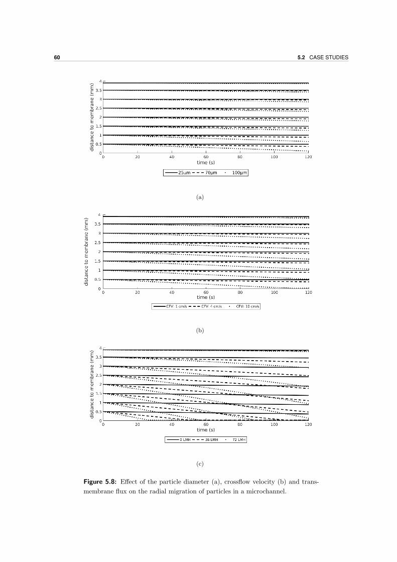
60 5.2 CASE STUDIES
(a)
(b)
(c)
Figure 5.8: Effect of the particle diameter (a), crossflow velocity (b) and trans-
membrane flux on the radial migration of particles in a microchannel.
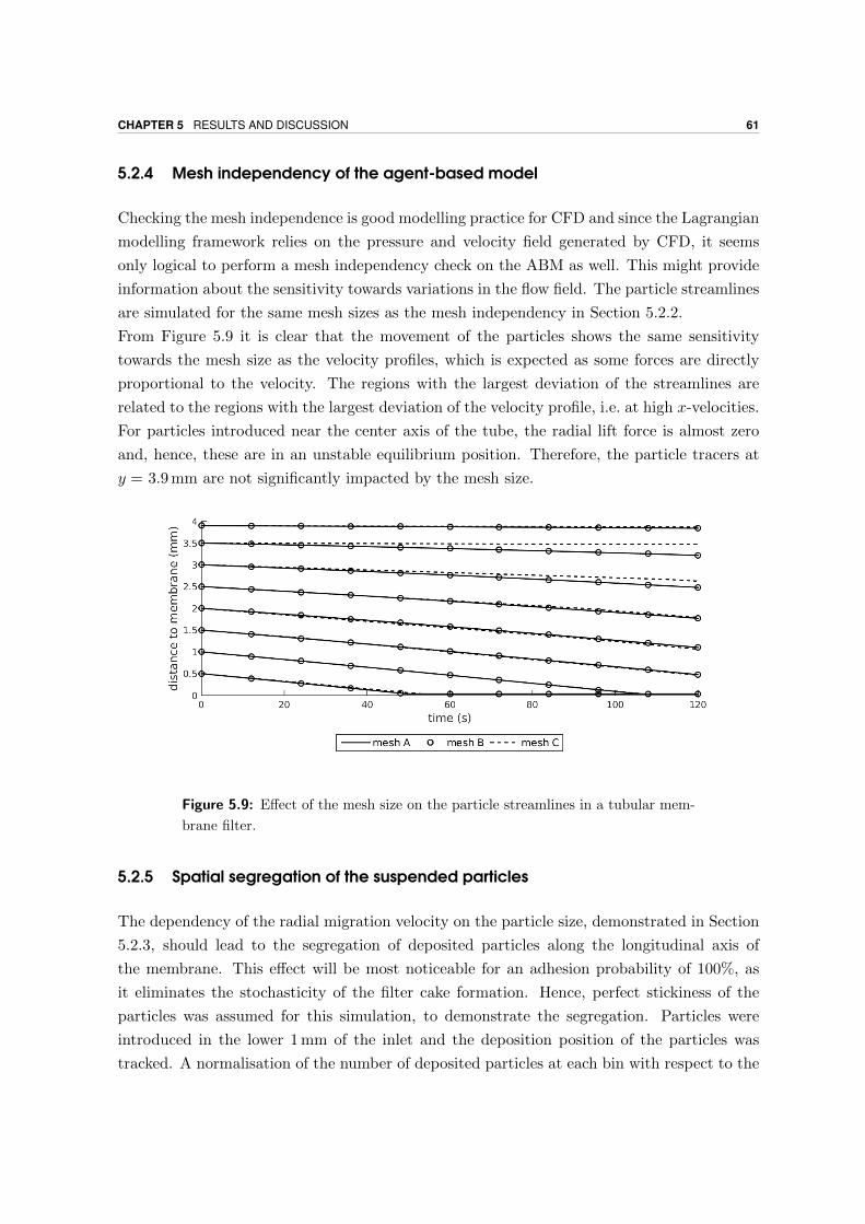
CHAPTER 5 RESULTS AND DISCUSSION 61
5.2.4 Mesh independency of the agent-based model
Checking the mesh independence is good modelling practice for CFD and since the Lagrangian
modelling framework relies on the pressure and velocity field generated by CFD, it seems
only logical to perform a mesh independency check on the ABM as well. This might provide
information about the sensitivity towards variations in the flow field. The particle streamlines
are simulated for the same mesh sizes as the mesh independency in Section 5.2.2.
From Figure 5.9 it is clear that the movement of the particles shows the same sensitivity
towards the mesh size as the velocity profiles, which is expected as some forces are directly
proportional to the velocity. The regions with the largest deviation of the streamlines are
related to the regions with the largest deviation of the velocity profile, i.e. at high x-velocities.
For particles introduced near the center axis of the tube, the radial lift force is almost zero
and, hence, these are in an unstable equilibrium position. Therefore, the particle tracers at
y = 3.9 mm are not significantly impacted by the mesh size.
Figure 5.9: Effect of the mesh size on the particle streamlines in a tubular mem-
brane filter.
5.2.5 Spatial segregation of the suspended particles
The dependency of the radial migration velocity on the particle size, demonstrated in Section
5.2.3, should lead to the segregation of deposited particles along the longitudinal axis of
the membrane. This effect will be most noticeable for an adhesion probability of 100%, as
it eliminates the stochasticity of the filter cake formation. Hence, perfect stickiness of the
particles was assumed for this simulation, to demonstrate the segregation. Particles were
introduced in the lower 1 mm of the inlet and the deposition position of the particles was
tracked. A normalisation of the number of deposited particles at each bin with respect to the
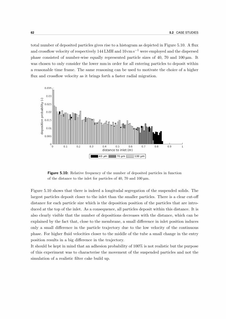
62 5.2 CASE STUDIES
total number of deposited particles gives rise to a histogram as depicted in Figure 5.10. A flux
and crossflow velocity of respectively 144 LMH and 10 cm s−1 were employed and the dispersed
phase consisted of number-wise equally represented particle sizes of 40, 70 and 100µm. It
was chosen to only consider the lower mm in order for all entering particles to deposit within
a reasonable time frame. The same reasoning can be used to motivate the choice of a higher
flux and crossflow velocity as it brings forth a faster radial migration.
Figure 5.10: Relative frequency of the number of deposited particles in function
of the distance to the inlet for particles of 40, 70 and 100µm.
Figure 5.10 shows that there is indeed a longitudal segregation of the suspended solids. The
largest particles deposit closer to the inlet than the smaller particles. There is a clear cut-off
distance for each particle size which is the deposition position of the particles that are intro-
duced at the top of the inlet. As a consequence, all particles deposit within this distance. It is
also clearly visible that the number of depositions decreases with the distance, which can be
explained by the fact that, close to the membrane, a small difference in inlet position induces
only a small difference in the particle trajectory due to the low velocity of the continuous
phase. For higher fluid velocities closer to the middle of the tube a small change in the entry
position results in a big difference in the trajectory.
It should be kept in mind that an adhesion probability of 100% is not realistic but the purpose
of this experiment was to characterise the movement of the suspended particles and not the
simulation of a realistic filter cake build up.

CHAPTER 5 RESULTS AND DISCUSSION 63
5.2.6 Effect of polydispersity
In order to assess the effect of polydispersity, a comparison was made between the filter cake
of a mono- and polydisperse bulk phase. This is also the ideal opportunity to perform a
full-fledged simulation with filter cake formation to identify the model imperfections.
The polydisperse simulation used an experimentally determined PSD of MBR sludge (Figure
5.4) and the monodisperse simulation used the number average particle size of this distribu-
tion, which was 40.82µm. The filter cake formation was simulated for 15 s and each scenario
was run four times in order to assess the stochastic nature of the model, which is depicted as
a band (average, minimum and maximum) in Figure 5.11. The average filter cake thickness
in time is presented in Figure 5.11 (a) and shows that polydispersity gives rise to a faster
filter cake build up. Section 5.2.5 demonstrates the fast deposition of big particles and, in
a polydisperse setting, these will “catch” smaller particles giving rise to a fast filter cake
development. This synergistic effect is not present in a monodisperse setting and the filter
cake is thereby formed at a slower pace. The evolution of the filter cake porosity is shown
in Figure 5.11 (b). Initially, there is no filter cake and the porosity is equal to one, and due
to the formation of filter cake patches the porosity starts decreasing at a higher rate in the
polydisperse setting. This could, however, be due to a denser filter cake or a higher surface
coverage, which cannot be determined from the figure. For this, the porosity of the actual
filter cake patches has to be evaluated (Figure 5.11 (c)). It can be seen that the filter cake in
the polydisperse setting is more densily packed than in the monodisperse case. As mentioned
previously, polydispersity should theoretically lead to a denser packing of the particles in the
filter cake. Hence, the simulation results are in agreement with the literature (Desmond and
Weeks, 2014; Sohn and Moreland, 1968).
However, these simulation results still have their imperfections. Figure 5.12 shows a two-
dimensional projection of the centers of the deposited particles after 2 min of simulation (the
monodisperse case). Note the unrealistic architecture of the filter cake, embodied by the
formation of narrow filter cake piles. This observation is confirmed by the longitudal variance
of the filter cake thickness, presented in Figure 5.11 (d). Hence, it can be concluded that the
problem of particles piling up was not resolved by transitioning to a three-dimensional model.
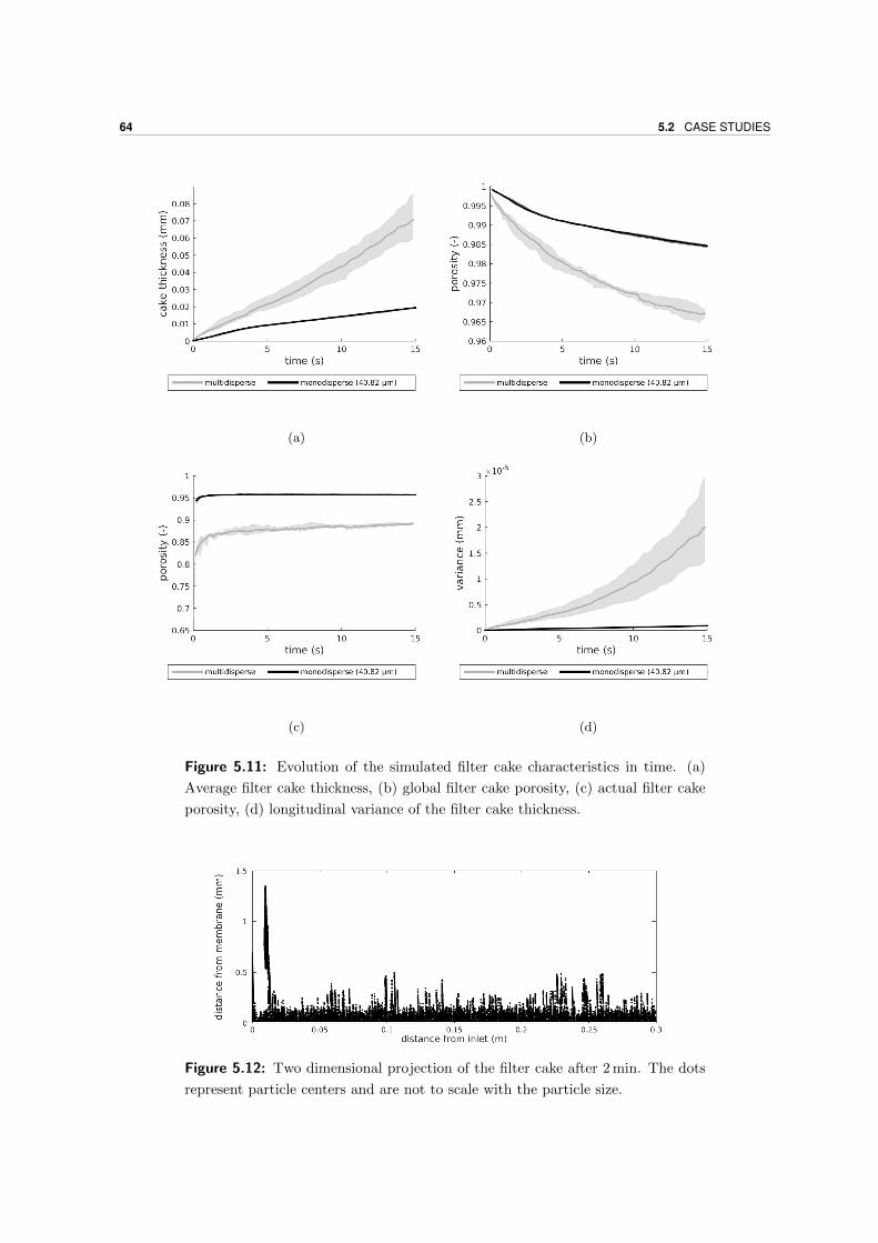
64 5.2 CASE STUDIES
(a) (b)
(c) (d)
Figure 5.11: Evolution of the simulated filter cake characteristics in time. (a)
Average filter cake thickness, (b) global filter cake porosity, (c) actual filter cake
porosity, (d) longitudinal variance of the filter cake thickness.
Figure 5.12: Two dimensional projection of the filter cake after 2 min. The dots
represent particle centers and are not to scale with the particle size.

CHAPTER 6General discussion and perspectives
Despite of the accomplished progress, the model still has a few shortcomings and it is impor-
tant to address these. Besides, looking forward, guidelines and remarks are provided for future
improvements. In the final part of this chapter, different sources of numerical instability are
mapped out and a brief discussion on the suitability of different profilometric techniques for
the specific task of characterising the filter cake is given.
6.1 Remarks on the bulk phase force balance
In Chapter 5, a qualitative validation is performed of the force balance in the model. The
results were mostly in agreement with the theoretical description of Matas et al. (2004) and
the experimental observations of Segre and Silberberg (1962) and Di Carlo et al. (2007). Still,
the absence of an equilibrium position raises questions about the integrity of the force balance
(Eq. (3.3)). The reason for this apparent shortcoming should be sought in the forces that
are able to counteract the radial migration of particles. Zeng et al. (2005) indicate that the
presence of a nearby wall breaks the axisymmetry of the wake vorticity distribution as well
as a tortuosity change, inducing a lift force that moves the particles away from the wall. This
mechanism is not explicitly included in the force balance but might be accounted for under
the guise of the Faxen correction:
Ur,eff = Ur −1
24d2
p∇2Uc , (6.1)
with Ur,eff [m s−1 ] the Faxen corrected relative velocity and Ur the actual relative velocity
of the particles. In two dimensions, the Laplacian of Eq. (6.1) can be written as,
∇2Uc =δ2Uc
δx2+δ2Uc
δy2. (6.2)

66 6.2 FILTER CAKE FORMATION
A fully developed Poiseuille (parabolic) flow is assumed in the tube. For this flow regime, the
second derivative of Uc with respect to y is constant along the width of the tube. Hence,
δ2Uc
δy2= c . (6.3)
Furthermore, Uc is constant with respect to x under these conditions, so
δ2Uc
δx2= 0 . (6.4)
Therefore,1
24d2p∇2Uc = c , (6.5)
and this shows that the Faxen correction is constant for a Poiseuille flow and is clearly not the
wall repulsion effect described by Zeng et al. (2005), which reaches a maximum magnitude
near the walls.
In order to increase the accuracy of the force balance, it might be interesting to investigate the
addition of the wall-induced lift force as it seems to have a considerable impact on the flow of
particles. Furthermore, next to Saffman’s lift force, two additional lift forces are described in
Matas et al. (2004); the shear gradient-induced lift force due to the curvature of the velocity
profile and the Magnus effect due to the forced rotation of the particles. It is likely that the
Magnus effect is negligible compared to the inertial lift force, but the shear gradient-induced
lift force might be of the same order of magnitude, and should therefore be investigated.
Due to the uncertainty of the magnitude of these forces and the complex nature of their
interaction with other operational variables, it is meaningful to first validate the model in
order to assess the necessity of an extension of the force balance.
6.2 Filter cake formation
The simulation results in Section 5.2.6 indicate the formation of filter cake towers, in spite of
the extension of the model to three dimensions. In order to resolve this unrealistic behavior,
a rolling algorithm should be included in the model. This will assure that only particles
that reach a stable position will attach to the filter cake. As mentioned previously, such a
framework is described in Cao et al. (2015) and should be assigned a high priority in the
further development of the model as it is imperative for the simulation of realistic filter cake
structures.
Next to the packing of particles, it is meaningful to reflect on the adhesion probability equa-
tion (Eq. (3.5)). Although this equation serves its purpose of constraining the filter cake
formation to low shear regions quite well, several arguments indicate the necessity for the
revision of this equation. Firstly, due to the stochastic nature of the model, there is always
a chance that particles adhere in high shear regions, and currently these particles remain

CHAPTER 6 GENERAL DISCUSSION AND PERSPECTIVES 67
attached indefinitely. Secondly, the simulations indicate a positive correlation of the radial
migration magnitude and the particle size, resulting in an easier filter cake formation for
bigger particles. This contradicts the experimental observations in Li et al. (1998). Hence,
it seems that Eq. (3.5) is not able to accurately simulate the balance between adhesion and
detachment of particles to the membrane or filter cake, which is a complex interplay between
particle-particle interactions (attachment to the filter cake), particle-interface interactions (at-
tachment to the membrane) and the liquid flow (shear at the membrane, compression due to
TMP, etc.). A theoretical foundation for particle-particle and particle-interface interactions
in dispersions is provided by the Derjaguin, Landau, Verwey and Overbeek (DLVO) theory,
which determines the balance between the electrostatic repulsion and the van der Waals at-
traction (Lyklema, 1968). However, the DLVO theory does not comprise all the necessary
processes for a complete representation of the interactions. The agglomeration of particles
is also influenced by hydration forces, steric forces and hydrophobic interactions (Van Oss,
1989; Hermansson, 1999). Finally, the hydrodynamics and pressure-driven effects should also
be accounted for as it is hypothesised that these effects greatly influence the formation of the
filter cake. It can be concluded that Eq. (3.5) is too simple for an accurate representation of
filter cake formation and it is clear why it does not yield satisfactory filter cake structures.
Moreover, a mechanistic approach in the form of a force balance over the particles in the filter
cake is imperative in order to simulate and comprehend backwashing and aeration processes.
6.3 Coupling ABM and continuous model
As mentioned in Chapter 3, the two model layers are coupled unidirectionally. The steady-
state flow profile of the continuous phase is calculated once at the beginning of the simulation
and is used throughout the whole simulation. Hence, the formation of the filter cake has no
impact on the continuous phase and the permeate keeps flowing unperturbed, regardless of
the fouling severity, which is not at all realistic. Two effects can be identified that demonstrate
the impact of filter cake on the surrounding fluid.
The first is the effect of the filter cake by increasing the filtration resistance. An increase in
filtration resistance due the presence of a porous filter cake in a certain region will make the
fluid move towards cleaner regions, which implies the spatial variation of the flux. Addition-
ally, the presence of a filter cake has an effect on the velocity of the surrounding fluid. Here,
it is not the flux that is affected, but rather the general flow profile. Both effects are currently
not included in the model but with for a realistic filter cake formation model, at least the
increasing filtration resistance should be considered.
To model this, a RIS approach can be applied with two resistance terms, the clean membrane
resistance (Rm) and the filter cake resistance (Rc):
Rtot = Rm +Rc , (6.6)

68 6.3 COUPLING ABM AND CONTINUOUS MODEL
where Rc can be obtained from:
Rc = l Kc, (6.7)
and Kc is obtained from:
Kc =K 90
dp
(ε)2
(1− ε)3. (6.8)
where Kc [m−2 ] is the specific cake resistance, l [m ] the filter cake thickness, K [ - ] the kozeny
constant, dp [m ] the mean particle diameter and ε [ - ] the filter cake porosity.
By plugging the total filtration resistance Rtot into Darcy’s law, an expression is obtained to
calculate the flux:
J =∆p
Rtot νf, (6.9)
The flux decrease could be considered homogeneously over the entire membrane. However,
the creation of a realistic filter cake architecture requires a spatially variable flux. So, a
sectional approach similar to Li and Wang (2006) should be used (Figure 6.1). Hence, the
membrane surface is subdivided in sections with a constant length (∆x). The flux through
each section is calculated with Eqs. (6.6)-(6.9). The newly calculated fluxes are subsequently
employed as boundary conditions on the membrane face and a new flow profile has to be
generated via CFD.
l
∆x
J
Figure 6.1: Schematic representation of a heterogeneously distruted flux along
the membrane surface.
In order to account for the variable flux, a bidirectional coupling has to be established between
CFD and the ABM, which is, however, not straightforward because both model layers are
implemented in different software platforms. Nonetheless, two approaches are identified to
establish such a coupling.

CHAPTER 6 GENERAL DISCUSSION AND PERSPECTIVES 69
The first approach involves using a third program as a wrapper that distributes the flux data
from MATLAB to OpenFOAM and the flow profile from OpenFOAM to MATLAB. This
approach is the most straightforward and can be accomplished by means of shell scripting. The
second approach involves setting up a MATLAB engine script in OpenFOAM that compiles
MATLAB’s m-code to C++. This approach is much more complex, but is computationally
very efficient.
In order to be able to account for the direct effects of the filter cake on the surrounding
liquid, it is necessary to explicitly model the suspended particles and the interactions with
the continuous phase. This can only be achieved with discrete element methods.
6.4 Sources of numerical instability
It is important to keep in mind that this spatio-temporal model basically consists of a system of
PDEs which are discretised and solved numerically. These methods can suffer from numerical
instabilities and this is also the case for this model. As it seems important for future work, a
brief overview is provided of the causes of numerical instability.
The first source of instability is described in Ghijs (2014) and concerns the Stokes drag force
which introduces a maximum solver time step limited by the smallest particle diameter, i.e.
∆t ≤ρp dp
2
18 νf. (6.10)
A second source of instability are the velocity fields from CFD. The convergence criteria of
the OpenFOAM solvers are set to 10−7 which means that openFOAM will stop iterating when
the difference between the fields of the current and previous iteration is smaller than 10−7.
This results in velocity fields where zeros are actually numbers between 10−8 and −10−8.
Although seemingly unimportant, this causes numerical instabilities due to the sensitivity of
the force balance to the sign of the fluid velocity. This issue can be easily solved by employing
a filter on the velocity values setting all values below the convergence criteria to zero.
Lastly, an additional constraint on the solver time step was found, this time originating for
large particles (dp > 100µm) in the system. Under high crossflow velocities and fluxes, the
radial migration of particles is a lot more prominent and forms another source of numerical
instability. Nevertheless, it is likely that for more extreme conditions this instability will also
impact smaller particles and it should be further investigated.
6.5 Profilometry
In Chapter 2, an overview was given of the prominent profilometric techniques along with
their lateral resolution and application restrictions. Based on this information, it is possible to
make a selection of the profilometers that are most suitable for the characterisation of the filter

70 6.5 PROFILOMETRY
cake surface. The filter cake should be characterised at micrometre scale, and techniques such
as AFM, SEM, STM are mostly used in the lower regions of the microscale and nanoscale.
Although a high resolution does not impose a direct problem, this implies a low surface
covering capacity and a high price tag, making these profilometers inappropriate for the task
at hand. The contact-based modus operandi of stylus profilometry can disturb the surface
of the soft filter cake and give rise to faulty measurements. Furthermore, white light axial
chromatism provides direct measurements of the distance, in contrast to the interferometry-
based techniques where the distance is derived from other measured quantities. Hence, it
seems that white light axial chromatism is the most suitable technique for profiling filter
cake.

CHAPTER 7Conclusion
Aiming at disclosing the mechanisms of filter cake formation, the model framework estab-
lished by Ghijs (2014) was succesfully extended. The representation of multidisperse feed
flows was implemented, enabling a realistic simulation of MBR feed flows characterised by a
PSD. Progression was made towards the formation of realistic filter cake structures by tran-
sitioning to a three-dimensional model. The implementation of a new filter cake attachment
algorithm and new sampling procedures induced an enhanced accuracy and computational
efficiency. Furthermore, the model implementation was parallelised, in order to speed-up the
calculations and a post-processing tool was developed for a user-friendly analysis of the simu-
lation results. The simulations of the extended model yielded interesting results and several
conclusions can be formulated.
First of all, an experimental microfiltration unit for the calibration and validation of the
model was designed by means of CFD. The unit presented a perfect laminar flow regime
without dead volumes or recirculation streams and enables a simplified representation of the
filtration unit, lowering the computational demand of the model. The CFD simulations indi-
cated that in order to obtain such a flow regime, a gradual transition from the inlet to the
membrane compartment is imperative.
Next, a qualitative validation showed that the model was able to reproduce the radial mi-
gration of non-buoyant particles in a Poiseuille flow, governed by the Segre-Silberberg effect.
The theoretically and experimentally acknowlegded dependency of the radial migration mag-
nitude on the Reynolds and particle Reynolds number was succesfully reproduced by the
model. However, the occurence of an equilibrium position at approximately 60 % of the
distance from the center axis to the wall was not observed. This is most likely due to the
absence of the wall-induced lift force in the force balance. Furthermore, the effect of the shear
gradient-induced lift force should also be investigated in order to determine its relevance for
filter cake formation. Through the Segre-Silberberg effect, a spatial segregation of the sus-
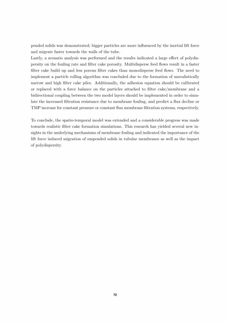
pended solids was demonstrated; bigger particles are more influenced by the inertial lift force
and migrate faster towards the walls of the tube.
Lastly, a scenario analysis was performed and the results indicated a large effect of polydis-
persity on the fouling rate and filter cake porosity. Multidisperse feed flows result in a faster
filter cake build up and less porous filter cakes than monodisperse feed flows. The need to
implement a particle rolling algorithm was concluded due to the formation of unrealistically
narrow and high filter cake piles. Additionally, the adhesion equation should be calibrated
or replaced with a force balance on the particles attached to filter cake/membrane and a
bidirectional coupling between the two model layers should be implemented in order to simu-
late the increased filtration resistance due to membrane fouling, and predict a flux decline or
TMP increase for constant pressure or constant flux membrane filtration systems, respectively.
To conclude, the spatio-temporal model was extended and a considerable progress was made
towards realistic filter cake formation simulations. This research has yielded several new in-
sights in the underlying mechanisms of membrane fouling and indicated the importance of the
lift force induced migration of suspended solids in tubular membranes as well as the impact
of polydispersity.
72
Bibliography
Bender, E. A. (2000). An Introduction to Mathematical Modeling. John Wiley & Sons, New
York, USA.
Binnig, G. and Rohrer, H. (1982). Scanning tunneling microscopy. Surface Science,
126(126):236–244.
Broeckmann, A., Busch, J., Wintgens, T., and Marquardt, W. (2006). Modeling of pore
blocking and cake layer formation in membrane filtration for wastewater treatment. De-
salination, 189(1-3):97–109.
Cao, T. A., Van De Staey, G., and Smets, I. Y. (2015). Integrating activated sludge floc size
information in MBR fouling modeling. Water Science & Technology, 71(7):1073–1080.
Catto, C. J. D. and Smith, K. C. A. (1973). Resolution limits in the surface scanning electron
microscope. Journal of Microscopy, 98(3):417–435.
Cha, S., Lin, P. C., Zhu, L., Sun, P. C., and Fainman, Y. (2000). Nontranslational three-
dimensional profilometry by chromatic confocal microscopy with dynamically configurable
micromirror scanning. Applied optics, 39(16):2605–2613.
Charcosset, C. (2014). Combining membrane processes with renewable energy technologies:
perspectives on membrane desalination, biofuels and biogas production, and microbial fuel
cells. In Membranes for Clean and Renewable Power Applications, pages 44–62. Elsevier.
Cheryan, M. and Rajagopalan, N. (1998). Membrane processing of oily streams. Wastewater
treatment and waste reduction. Journal of Membrane Science, 151(1):13–28.
Cimini, A., Marconi, O., and Moresi, M. (2013). Rough beer clarification by crossflow mi-
crofiltration in combination with enzymatic and/or centrifugal pretreatments. Chemical
Engineering Transactions, 32(2013):1729–1734.
Conroy, M. and Armstrong, J. (2005). A comparison of surface metrology techniques. Journal
of Physics: Conference Series, 13(2005):458–465.

Cross, M., Douglas, W. H., and Fields, R. P. (1985). Optimal design methodology for com-
posite materials with particulate fillers. Powder Technology, 43(1985):27–36.
Dalmau, M., Atanasova, N., Gabarron, S., Rodriguez-Roda, I., and Comas, J. (2015). Com-
parison of a deterministic and a data driven model to describe MBR fouling. Chemical
Engineering Journal, 260(2015):300–308.
Desmond, K. W. and Weeks, E. R. (2014). Influence of particle size distribution on random
close packing of spheres. Physical Review E, 90(2):022204.
Di Carlo, D., Irimia, D., Tompkins, R. G., and Toner, M. (2007). Continuous inertial focusing,
ordering, and separation of particles in microchannels. Proceedings of the National Academy
of Sciences of the United States of America, 104(48):18892–7.
Drews, A., Arellano-Garcia, H., Schoneberger, J., Schaller, J., Wozny, G., and Kraume, M.
(2009). Model-based recognition of fouling mechanisms in membrane bioreactors. Desali-
nation, 236(1-3):224–233.
Dube, M. A., Tremblay, A. Y., and Liu, J. (2007). Biodiesel production using a membrane
reactor. Bioresource Technology, 98(3):639–647.
Faxen, H. (1922). Der Widerstand gegen die Bewegung einer starren Kugel in einer zahen
Flussigkeit, die zwischen zwei parallelen ebenen Wanden eingeschlossen ist. Annalen der
Physik, 373(10):89–119.
Fu, F. and Wang, Q. (2011). Removal of heavy metal ions from wastewaters: A review.
Journal of Environmental Management, 92(3):407–418.
Ghijs, M. (2014). Spatio-temporal modeling of filter cake formation in membrane bioreactors.
Master thesis, Ghent university.
Goldstein, J. I., Newbury, D. E., Echlin, P., Joy, D. C., Lyman, C. E., Lifshin, E., Sawyer,
L., and Michael, J. R. (2003). Scanning Electron Microscopy and X-ray Microanalysis.
Springer US, Boston, MA, third edition.
Gorthi, S. S. and Rastogi, P. (2010). Fringe projection techniques: Whither we are? Optics
and Lasers in Engineering, 48(2):133–140.
Hansma, P. K. and Tersoff, J. (1987). Scanning tunneling microscopy. Journal of Applied
Physics, 61(2).
Hariharan, P. (2012). Basics of Interferometry. In Basics of Interferometry, page 213. Aca-
demic Press, San Diego, USA, first edition.
Hermansson, M. (1999). The DLVO theory in microbial adhesion. Colloids and Surfaces B:
Biointerfaces, 14(1-4):105–119.
74
Hocken, R., Chakraborty, N., and Brown, C. (2005). Optical Metrology of Surfaces. CIRP
Annals - Manufacturing Technology, 54(2):169–183.
Homsy, A., van der Wal, P. D., Doll, W., Schaller, R., Korsatko, S., Ratzer, M., Ellmerer,
M., Pieber, T. R., Nicol, A., and de Rooij, N. F. (2012). Development and validation of
a low cost blood filtration element separating plasma from undiluted whole blood. Biomi-
crofluidics, 6(1):1–9.
Hubbard, P. M. (1996). Approximating polyhedra with spheres for time-critical collision
detection. ACM Transactions on Graphics, 15(3):179–210.
Judd, S. (2008). The status of membrane bioreactor technology. Trends in Biotechnology,
26(2):109–116.
Judd, S. (2011). The MBR Book: Principles and Applications of Membrane Bioreactors for
Wastewater Treatment. Elsevier Ltd, Oxford, UK, second edition.
Kemper, B., Langehanenberg, P., and von Bally, G. (2007). Digital holographic microscopy:
a new method for surface analysis and marker-free dynamic life cell imaging. Optik &
Photonik, 2(2):41–44.
Khalaf, R. M. F. and Bainbridge, D. R. (1981). Nomarski differential interference contrast
studies of murine lymphocytes. European Journal of Immunology, 11(10):816–824.
Khan, S. J., Visvanathan, C., and Jegatheesan, V. (2009). Prediction of membrane fouling in
MBR systems using empirically estimated specific cake resistance. Bioresource Technology,
100(23):6133–6136.
Koros, W. J., Ma, Y. H., and Shimidzu, T. (1996). Terminology for membranes and membrane
processes (IUPAC Recommendations 1996). Pure and Applied Chemistry, 68(7):149–159.
Leach, R. (2011). Optical Measurement of Surface Topography. Springer Berlin Heidelberg,
Heidelberg, Berlin, first edition.
Li, H., Fane, A., Coster, H., and Vigneswaran, S. (1998). Direct observation of particle
deposition on the membrane surface during crossflow microfiltration. Journal of Membrane
Science, 149(1):83–97.
Li, X. Y. and Wang, X. M. (2006). Modelling of membrane fouling in a submerged membrane
bioreactor. Journal of Membrane Science, 278(1-2):151–161.
Lonardo, P., Lucca, D., and De Chiffre, L. (2002). Emerging Trends in Surface Metrology.
CIRP Annals - Manufacturing Technology, 51(2):701–723.
Lu, W.-M. and Hwang, K.-J. (1993). Mechanism of cake formation in constant pressure
filtrations. Separations Technology, 3(3):122–132.
75

Luque, S., Gomez, D., and Alvarez, J. R. (2008). Industrial Applications of Porous Ceramic
Membranes (PressureDriven Processes). Membrane Science and Technology, 13(7):177–216.
Lyklema, J. (1968). Principles of the stability of lyophobic colloidal dispersions in non-aqueous
media. Advances in Colloid and Interface Science, 2(2):67–114.
Maere, T., Villez, K., Marsili-Libelli, S., Naessens, W., and Nopens, I. (2012). Membrane
bioreactor fouling behaviour assessment through principal component analysis and fuzzy
clustering. Water Research, 46(18):6132–6142.
Matas, J. P., Morris, J. F., and Guazzelli, E. (2004). Lateral forces on a sphere. Oil and Gas
Science and Technology, 59(1):59–70.
MathWorks (2016). MATLAB web page. http://nl.mathworks.com/products/matlab/.
Accessed: 20-04-2016.
Maxey, M. R. and Riley, J. J. (1983). Equation of motion for a small rigid sphere in a
nonuniform flow. Physics of Fluids, 26(1983):883.
Meng, F., Zhang, H., Yang, F., Zhang, S., Li, Y., and Zhang, X. (2006). Identification of
activated sludge properties affecting membrane fouling in submerged membrane bioreactors.
Separation and Purification Technology, 51(1):95–103.
Mirbagheri, S. A., Bagheri, M., Bagheri, Z., and Kamarkhani, A. M. (2015). Evaluation and
prediction of membrane fouling in a submerged membrane bioreactor with simultaneous
upward and downward aeration using artificial neural network-genetic algorithm. Process
Safety and Environmental Protection, 96:111–124.
Mohammadi, T., Madaeni, S. S., and Moghadam, M. K. (2003). Investigation of membrane
fouling. Desalination, 153:155–160.
Naessens, W., Maere, T., and Nopens, I. (2012). Critical review of membrane bioreactor
models - Part 1: Biokinetic and filtration models. Bioresource Technology, 122:95–106.
Nanovea (2015). Chromatic confocal profilometers, technical sheet. http://nanovea.com/
wp-content/themes/wp-nanovea/brochures/profilers.pdf. Accessed: 13-02-2016.
Open-Cascade (2016). SALOME web page. http://www.salome-platform.org/. Accessed:
20-04-2016.
OpenFOAM-Foundation (2016). OpenFOAM web page. http://openfoam.com/. Accessed:
20-04-2016.
Owen, G., Bandi, M., and Howell, J. A. (1995). Economic assessment of membrane processes
for water and waste water treatment. 102:77–91.
76
Patankar, S. (1980). Numerical Heat Transfer and Fluid Flow. Hemisphere Publishing Cor-
poration, first edition.
Pawley, J. B. (1995). Handbook of Biological Confocal Microscopy. Springer Science & Business
Media, New York, USA, second edition.
Picioreanu, C., Vrouwenvelder, J., and van Loosdrecht, M. (2009). Three-dimensional model-
ing of biofouling and fluid dynamics in feed spacer channels of membrane devices. Journal
of Membrane Science, 345(1-2):340–354.
Podoleanu, A. G. (2012). Optical coherence tomography. Journal of Microscopy, 247(3):209–
219.
Prasad, N. K. (2010). Downstream Process Technology: A New Horizon in Biotechnology.
Prentice-Hall Of India Pvt. Limited, New Delhi, India.
Python-Software-Foundation (2016). Python web page. https://www.python.org/. Ac-
cessed: 20-04-2016.
Ranade, V. V. (2002). Computational flow modeling for chemical reactor engineering. Aca-
demic Press, Massachusetts, USA.
Reimer, L. (1985). Scanning Electron Microscopy. Springer Berlin Heidelberg, Berlin, Hei-
delberg.
Roache, P. J. (1997). Quantification of Uncertainty in Computational Fluid Dynamics. Annual
Review of Fluid Mechanics, 29(1):123–160.
Rossler Tomas, Hrabovsky, M., Jiri, K., and Bartonek, L. (1998). Control of pump blade by
moire topography fringe-shifting method. In Optical Conference On Wave and Quantum
Aspects of Contemporary Optics Proceedings, pages 161–168.
Saffman, P. G. (1965). The lift on a small sphere in a slow shear flow. Journal of Fluid
Mechanics, 22(02):385.
Scott, K. and Highes, R. (2012). Industrial Membrane Separation Technology. Springer
Science & Business Media, Dordrecht, Netherlands, first edition.
Segre, G. and Silberberg, A. (1961). Radial Particle Displacements in Poiseuille Flow of
Suspensions. Nature, 189(4760):209–210.
Segre, G. and Silberberg, A. (1962). Behaviour of macroscopic rigid spheres in Poiseuille
flow Part 1. Determination of local concentration by statistical analysis of particle passages
through crossed light beams. Journal of Fluid Mechanics, 14(01):115.
77
Shetty, G. R. and Chellam, S. (2003). Predicting membrane fouling during municipal drinking
water nanofiltration using artificial neural networks. Journal of Membrane Science, 217(1-
2):69–86.
Sohn, H. Y. and Moreland, C. (1968). The effect of particle size distribution on packing
density. The Canadian Journal of Chemical Engineering, 46(3):162–167.
Song, J. (1991). Stylus profiling at high resolution and low force. Applied optics, 30(1):42–50.
Stout, K. and Blunt, L. (2000). Three Dimensional Surface Topography. Elsevier.
Su, X. and Chen, W. (2001). Fourier transform profilometry: A review. Optics and Lasers
in Engineering, 35(5):263–284.
Tamime, A. Y. (2012). Membrane Processing: Dairy and Beverage Applications. John Wiley
& Sons, Chichester, UK, first edition.
Taylor, J. B., Carrano, A. L., and Kandlikar, S. G. (2006). Characterization of the effect of
surface roughness and texture on fluid flowpast, present, and future. International Journal
of Thermal Sciences, 45(10):962–968.
Tu, J. V. (1996). Advantages and disadvantages of using artificial neural networks ver-
sus logistic regression for predicting medical outcomes. Journal of Clinical Epidemiology,
49(11):1225–1231.
Ulbricht, M., Ansorge, W., Danielzik, I., Konig, M., and Schuster, O. (2009). Fouling in mi-
crofiltration of wine: The influence of the membrane polymer on adsorption of polyphenols
and polysaccharides. Separation and Purification Technology, 68(3):335–342.
Van Oss, C. J. (1989). Energetics of cell-cell and cell-biopolymer interactions. Cell Biophysics,
14(1):1–16.
Versteeg, H. and Malalasekera, W. (1995). An Introduction to Computational Fluid Dynamics
- The Finite Volume Method. Longman Scientific & technical, London, UK, first edition.
Vrouwenvelder, J. S., Picioreanu, C., Kruithof, J. C., and van Loosdrecht, M. C. M. (2010).
Biofouling in spiral wound membrane systems: Three-dimensional CFD model based eval-
uation of experimental data. Journal of Membrane Science, 346(1):71–85.
Whitehouse, D. (1999). Surface metrology. Computer Standards & Interfaces, 21(2):185.
Wintgens, T., Rosen, J., Melin, T., Brepols, C., Drensla, K., and Engelhardt, N. (2003).
Modelling of a membrane bioreactor system for municipal wastewater treatment. Journal
of Membrane Science, 216(1-2):55–65.
78

Worner, M. (2003). A Compact Introduction to the Numerical Modeling of Multiphase Flows.
Technical report, Karlsruhe, Germany.
Yoon, S., Lee, C., Kim, K., and Fane, A. G. (1999). Three-dimensional simulation of the
deposition of multi-dispersed charged particles and prediction of resulting flux during cross-
flow microfiltration. Journal of Membrane Science, 161:7–20.
Zeng, L., Balachandar, S., and Fischer, P. (2005). Wall-induced forces on a rigid sphere at
finite Reynolds number. Journal of Fluid Mechanics, 536:1–25.
Zhang, S. (2010). Recent progresses on real-time 3D shape measurement using digital fringe
projection techniques. Optics and Lasers in Engineering, 48(2):149–158.
Zikanov, O. (2010). Essential Computational Fluid Dynamics. John Wiley & Sons, Hoboken,
USA, first edition.
79

80

APPENDIX ATechnical drawing microfilter
A-A ( 1 : 4 )
1
1
2
2
3
3
4
4
5
5
6
6
A A
B B
C C
D D
plexy-bovenkant
mpodevyn 27-11-2015
Designed by Checked by Approved by Date
1 / 1 Edition Sheet
Date
A
A
15
19
25
750
150
43,5
4
M20x1.5 - 6
H
30
10
40
9R10
R15
100
28,5
Figure A.1: Technical drawing of the microfiltration device
81