Spatio-Temporal GeostatisticalModels, with an Application in

Fish Stock

Ioannis Elmatzoglou

Submitted for the degree of Master in Statisticsat Lancaster University,

September 2006.

Abstract

Geostatistics is based on the adoption of a probabilistic framework, aiming atthe description of the behavior of any kind of continuous and quantifiable spa-tial phenomenon. However, many such phenomena are characterized not onlyby spatial but also by temporal variability. Although geostatistics was initiallydeveloped for the needs of the mining industry, it is now used in many otherapplication areas including hydrological, environmental and meteorological ap-plications. Although spatio-temporal analysis is in princilpe a direct extensionof the geostatistical philosophy of analysis in space, in practice there are manyobstacles in the path to its full development.

II

Acknowledgements

Many thanks to my supervisor Paulo J. Ribeiro for his help, his guidelines andhis general contribution to my knowledge. 1000 thanks to Peter Diggle for thetime he spent and the great interest that he showed to make improvements in myproject. The quality and the organization of the data analysis would be muchdifferent without his suggestions. It is in general a great honor for me to workwith people like him. I would also like to thank: Martin Schlather for the helphe provided in aspects concerning the comprehension of RandomFields software.The Department of Statistics of Lancaster University for the funding coveringmy tickets to Brazil and studentship offered to me through the academic year2005-2006. Loukia Meligkotsidou for her willingness to help at a really verybad moment, even though see didn’t. My father Antonios Elmatzoglou for hissupport and last, many thanks to George Tsiotas, Department of Economics,University of Crete, as without him I wouldn’t be here doing anything.

III

Contents

1 An Introduction to Geostatistics 11.1 From Classical Statistics to Geostatistics . . . . . . . . . . . . . . 1

1.1.1 A Motivating Example . . . . . . . . . . . . . . . . . . . . 11.1.2 Geostatistics . . . . . . . . . . . . . . . . . . . . . . . . . 1

1.2 Approaches in Geostatistical Analysis . . . . . . . . . . . . . . . 21.3 Geostatistics in Space and Time . . . . . . . . . . . . . . . . . . 31.4 What follows . . . . . . . . . . . . . . . . . . . . . . . . . . . . . 3

2 Geostatistical Analysis of Spatial Data 42.1 Introduction . . . . . . . . . . . . . . . . . . . . . . . . . . . . . . 42.2 Basics . . . . . . . . . . . . . . . . . . . . . . . . . . . . . . . . . 42.3 Special Characterizations of Random Fields . . . . . . . . . . . . 6

2.3.1 Stationary Random Fields . . . . . . . . . . . . . . . . . . 62.3.2 Non-Stationary Random Fields . . . . . . . . . . . . . . . 72.3.3 Anisotropy . . . . . . . . . . . . . . . . . . . . . . . . . . 72.3.4 Gaussian Random Fields (GRF) . . . . . . . . . . . . . . 9

2.4 Modeling the Dependency Structure . . . . . . . . . . . . . . . . 92.4.1 Properties of Second-Order Covariance functions . . . . . 102.4.2 Covariance Models . . . . . . . . . . . . . . . . . . . . . . 102.4.3 Spectral Representation . . . . . . . . . . . . . . . . . . . 112.4.4 Nesting of Covariance Models . . . . . . . . . . . . . . . . 12

2.5 Parameter Estimation and Predictions . . . . . . . . . . . . . . . 132.5.1 Estimation with Variograms . . . . . . . . . . . . . . . . . 132.5.2 Maximum Likelihood Estimation . . . . . . . . . . . . . . 142.5.3 Predictions and Kriging . . . . . . . . . . . . . . . . . . . 15

3 Models for spatio-temporal geostatistical data 163.1 Introducing the New Dimension . . . . . . . . . . . . . . . . . . . 163.2 Different Approaches in the Spatio-Temporal Analysis . . . . . . 163.3 Nesting of Space-Time Covariance Functions . . . . . . . . . . . 173.4 Separable Space-Time Models . . . . . . . . . . . . . . . . . . . . 18

3.4.1 Some Examples of separable models . . . . . . . . . . . . 183.5 Non-Separable Models . . . . . . . . . . . . . . . . . . . . . . . . 193.6 Stationary Space-Time Models . . . . . . . . . . . . . . . . . . . 193.7 Anisotropy? . . . . . . . . . . . . . . . . . . . . . . . . . . . . . . 193.8 Fully-Symmetry . . . . . . . . . . . . . . . . . . . . . . . . . . . . 19

3.8.1 Not Fully-Symmetric Space-Time Covariance Models . . . 20

IV

CONTENTS V

3.9 Simulations of Simple Spatio-Temporal Gaussian Random Fieldswith Different Dependency Features . . . . . . . . . . . . . . . . 213.9.1 Simulating a Random Field with a Non-Separable and

Fully Symmetric Covariance Function . . . . . . . . . . . 223.9.2 Simulating a Random Field with a Non-Separable and

Not Fully-Symmetric Covariance Function . . . . . . . . . 233.9.3 Simulating two Random Fields with a Separable Depen-

dency Structure . . . . . . . . . . . . . . . . . . . . . . . . 233.10 Realism vs. Convenience . . . . . . . . . . . . . . . . . . . . . . . 243.11 The Creesie-Huang Approach . . . . . . . . . . . . . . . . . . . . 263.12 Gneiting’s Family of Non-Separable Models . . . . . . . . . . . . 26

4 Case Study: Spatio-Temporal Modeling of the Portuguese FishStocks 284.1 Introduction . . . . . . . . . . . . . . . . . . . . . . . . . . . . . . 284.2 Scientific Interest and Data Description . . . . . . . . . . . . . . 284.3 The Need for Joint Space-Time Analysis . . . . . . . . . . . . . . 294.4 Methods . . . . . . . . . . . . . . . . . . . . . . . . . . . . . . . . 294.5 Exploratory Data Analysis and Assumptions . . . . . . . . . . . 304.6 Analysis . . . . . . . . . . . . . . . . . . . . . . . . . . . . . . . . 32

4.6.1 Comparison between the Purely Spatial Models AssumingConstant and Non-Constant Properties Over Time . . . . 33

4.6.2 Purely Temporal Analysis . . . . . . . . . . . . . . . . . . 344.6.3 Building a Space-Time Covariance Model and Testing its

Superiority over the Purely Spatial one . . . . . . . . . . 344.6.4 Construction of a Gneiting ’s type Non-Separable Covari-

ance Model and Testing its Appropriateness against theSeparable one . . . . . . . . . . . . . . . . . . . . . . . . . 36

4.7 Time-Forward Kriging Assessment with the two Models . . . . . 394.8 Assessment and conclusions . . . . . . . . . . . . . . . . . . . . . 43

5 Concluding Remarks and Further Studies 44

6 Appendices 476.1 Appendix A . . . . . . . . . . . . . . . . . . . . . . . . . . . . . . 47

6.1.1 Simulations from the Estimated Model and Variability ofEstimations, (See Appendix B for Rcodes) . . . . . . . . . 47

6.2 Appendix B . . . . . . . . . . . . . . . . . . . . . . . . . . . . . . 486.2.1 R CODES . . . . . . . . . . . . . . . . . . . . . . . . . . . 48

6.3 Simulating from the Estimated Model and Computation of theP.Likelihood of the Seperability Parameter . . . . . . . . . . . . . 50

September 27, 2006

Chapter 1

An Introduction to Geostatistics

1.1 From Classical Statistics to Geostatistics

1.1.1 A Motivating Example

Suppose that our interest lies in predicting the average temperature V after one day, in the location A.What a statistician could do is treating all the average daily temperatures Vt in ”A” as random and thinkthat their values are closely related with each other. So a solution to our problem can be given by consideringall the past daily realized values of V : (vt−1, vt−2, . . . , vt−n) as an observed realization of a stochastic process,with a particular dependency structure. By exploring, through our sample, the way that these variables arerelated, we are enabled to express an opinion about the future, yet unrealized value of Vt+1.

Suppose that we are now interested in the amount of the underground oil deposits ”O” that exists in thelocation ”B” in a geographical area with many oil wells installed. Again, statistically thinking we can expressour ignorance about OB and think that its ”real” value, will be a realization from a certain probability dis-tribution. Unfortunately, we can’t use the same methodology. First of all, the expense of making excavationsis by far higher than the one when measuring the temperature. Second, the amount of the undergroundoil is going to be practically the same over time unless we don’t refine it. Thus, even if we could cheaplycheck the amount of oil in ”B”, this has no practical point as it is going to be constant over time. So, wedon’t have any information for this spatial location coming from different time instances. Due to this lack ofsamples in time, one thing that someone could do is trying to look for the ”existence” of some other kindsof information. This time, though, not coming from time but from space. And more specifically we can bebased on the information provided by the nearby existing oil wells. Smililarly, like before, we can think thatthe information coming from the closest wells is going to be more valuable than the ones that are far apart.This can give us the idea of working in the same kind of framework like before, with the temperature example.That is, to think that the underground oil deposit in all the locations of the area, is a sequence of infinitedependent random variables, indexed by Osi, and our sample as one particular realization os1, os2, . . . , osn atsome specific points. By exploring the way that they are linked, we are enabled to express an opinion for theamount of the yet unrealized, oil deposit in B.

The methodology in the two examples was quite similar, with the only difference being the sample source.In the first case this came from time , while in the second one it came from space. While the former can begiven as an example of time-series analysis, the latter is just a typical example of a geostatistical application.

1.1.2 Geostatistics

Geostatistics can be roughly thought of as the spatial version of time series and it is one of the three mainbranches of spatial statistics. It usually refers to the case where data consist of a finite sample of measuredvalues relating to an underlying spatially continuous phenomenon (Diggle & Ribeiro 2006 ). Example of this,can be the temperature in a particular area, the concentrations of a particular pollutant in the soil of a biggeographical region or even the wind’s velocity in the same location.

The first law of geography says that ”everything is related to everything else, but near things are morerelated than distant things” (Tobler, 1970, p.236 ). However, this seems to be in a great correspondencewith our temperature example, as the real and unknown value of the latter is more likely to be similar with

1

1.2.Approaches in Geostatistical Analysis 2

its measurements one or two days ago, than the ones one or two weeks before. In a similar manner, theinformation we get from the nearby wells is more likely to be more useful than one coming from the wellsfurther apart.

Although statistics has a well established methodology that allows for the description of the relationshipsbetween various random variables, geostatistics is a science independently developed. The term geostatisticswas firstly introduced by George Matheron (1962), as a means of designating his own methodology of orereserve evaluation. The same person coined the term regionalised variable to designate a numerical functionz(x) depending on a continuous space index x, and combining high irregularity of detail with spatial corre-lation. Being based on these words, Chiles and Delfiner (1999) defined Geostatistics as ”the application ofprobabilistic methods to regionalized variables”, which is different from the vague usage of the word in thesense statistics in Geosciences.

However, the range of applicability of this methodology has not been restricted by the concept attributedby the Greek prefix geo (γεω=earth,ground,soil,land) which emphasize the spatial aspect of the problem.Applications have been taken place into a wider class of environments such as the subsurface, land , atmosphereor oceans. This of course implies that there are more sciences involved with geostatistics than just thegeosciences. At this point it should be noted that geostatistics is just a complementary and biased tool ofperforming a spatial analysis. This can become clearer with the following example. Suppose that a bankis robbed in a particular region, say A. The fact that this happened in A and not in B can be interpretedby various ways from different people. It is sure that the interpretations of an economist, a psychologist, acriminologist , a sociologist and a policeman are going to be much different from each other. The same holdsin the case of Geosciences. The fact that region A is richer in mineral resources than B, it can be interpretedin a different way by a geologist or a physician.

Here it should be emphasized that geostatistics does not aim into the interpretation of what has beenobserved but it focuses mostly on making a description. It just aims to solve particular problems by capturingthe main structural features from the data. Its essence is to recognize the inherent variability of naturalspatial phenomena and the fragmentary character of the data and to incorporate these notions in a modelof stochastic nature. That means that it does not attempt any physical or genetic interpretation of the data(Chiles and Delfiner 1999) and knowledge of the subject matter does not have much impact in the analysis.And that, of course, means that data play unique role in the analysis. In our oil example, the non-existenceof other nearby wells implies that the problem is clearly converted to a geological one.

1.2 Approaches in Geostatistical Analysis

Traditional and Model Based Geostatistics

We mentioned earlier that geostatistics was an independently developed science , which later adopted manystatistical features. One consequence of this fact is that it still uses various non-formal statistical and adhoc methods of inference, such as fitting lines to variograms or ”fit by eye” methods. Main characteristicis the focus around the covariance structure of a given process that is usually assumed to have a Gaussiandistribution.

Diggle, Tawn & Moyeed (1998) coined the phrase model-based geostatistics to describe an approach togeostatistical problems based on the application of formal statistical methods under an explicitly assumedstochastic model. In this approach the covariance structure depends and it is a consequence of the modelassumed. In this project we follow the traditional approach.

Convolution Representation

A third alternative representation of a spatial process can be gained in the terms of convolutions. This isa completely different approach in which the spatial process is assumed to be constructed by integrating anunobserved and weighted white noise process, usually referred to as the excitation field. Such kind of repre-sentation has sometimes many advantages, such as an alternative way of deriving valid covariance functions,among some others. However, we are not going to pay much attention on this approach during this work.

1.3.Geostatistics in Space and Time 3

1.3 Geostatistics in Space and Time

Although in the case of oil deposits, the latter remain practically constant over time, when the interestlies in other kinds of processes such as nitrate nitrogen (NO3) contamination in groundwater or ammoniumnitrogen (NH4) contents in soil, the quality analysis can be much more enhanced by making more complexassumptions. In particular, models taking into account the fact that the process evolves not only in spacebut in time as well, are very often proved to be more useful. One main reason is that past information cancontribute not only in the improvement of the spatial interpolations at the present time, but also in our abilityto perform time-forward predictions at different spatial locations.

The modeling of spatiotemporal distributions resulting from dynamic processes evolving in both space andtime is critical and has been increasingly used in many scientific and engineering fields, involving environmentalsciences, climate prediction, meteorology, hydrology and reservoir engineering. Just as in the purely spatialcase, geostatistical spatiotemporal models provide a probabilistic framework for data analysis and predictionsthat builds on the joint spatial and temporal dependence between the observations. The simultaneous analysisof space and time is based exactly on the same philosophy as the analysis only in space. Time can be justtreated as an extra dimension in space. However, the fact that space and time are two completely differentnotions does not allow us treating them in an exact equivalent manner. For this reason the spatio-temporalanalysis and modeling has its own idiomorphies and difficulties, which makes it dependent on a further numberof assumptions.

1.4 What follows

The fact that joint space and time analysis needs to be treated in its own particular way, is the reason thatwe decided to split the analysis into two parts. As the title of the project implies and so, as our main concernin this project is the modeling of spatial processes at different time instances, we are initially focusing onmaking a brief description of the most necessary elements and main assumptions relating to the modeling ofthe purely spatial processes (Chapter 2 ). These elements are going to be useful in the next part, where weemphasize and focus on the additional characteristics that a space-time modeling has to encounter (Chapter3 ). In the last part of the project we make an application of the theory introduced earlier to a real problem(Chapter 4 ). So, to summarize, the work can be divided into three parts: two parts of theoretical analysisand one of application.

Chapter 2

Geostatistical Analysis of Spatial Data

2.1 Introduction

Main objective of this chapter is just to provide with a very short review of the main characteristics governingrandom fields existing in the purely spatial domain. This will enable us taking all the necessary ingredients inorder to understand the more complex assumptions characterizing the spatio-temporal processes. The chapterbegin with some very simple definitions, such as moments, variance and covariance structure of random fieldsand it continues by focusing on some very common and convenient assumptions such as, stationarity andisotropy. The rest of this chapter is concerned about different ways of modeling the dependency structureand different strategies for inference. Significant amount from the material presented below is inspired by thedescriptions of Le & Zidek (2006), Schabenberger & Gotway (2005) and Journel & Kyriakidhs (1999) as well.

2.2 Basics

A stochastic process is a family or collection of random variables, the members of which can be identifiedor located (indexed) according to some metric. Consider for convenience the first example of the previouschapter, where the measured value of the temperature P at each time point t1, . . . , tq was treated as arealization from a stochastic process that was considered to exist in time. While this kind of process is usuallyreferred to as a time-series process, a spatial process is defined to be a collection of random variables thatexist exclusively in the space domain. These variables are indexed by some set D ⊂ <d containing spatialcoordinates s = s1, . . . , sd. Our second example, regarding the prediction of the underground oil depositsin particular location we had two spatial coordinates i.e. s = (x1, x2) and so d = 2 , where D denotedthe particular geographical sub-region of interest. We could have also taken into account the depth of ourmeasurements and thus work in three dimensions (d = 3). In the case where d ≥ 1, the spatial process isusually referred to as random field. Each of the random ”components” of the field, Z(s), is fully characterizedby its cumulative distribution function (cdf ).

F (s; z) = Prob{Z(s) ≤ z}, ∀z and s ∈ <d

In other words, the previous expression gives the probability that the variable Z at the location s in space isnot greater than any given threshold z. Consider now the discretization of the d -dimensional spatial domain Dinto a set N of n points (N ⊆ D). The joint uncertainty about this n set of random variables is characterizedby the joint n-variate cdf :

F (s1, . . . , sn; z1, . . . , zn) = Prob{Z(s1) ≤ z1, . . . , Z(sn) ≤ zn}, si ∈ <d (2.1)

The random field is characterized by all these sets of n-dimensional distributions of random variables spatiallydefined by every possible discretized subset N . Gaussian Random Field (GRF) is defined to be thecase when all these joint distributions are multivariate Gaussians. This always implies that the marginaldistribution is Gaussian as well, while the inverse does not necessarily hold.

At this point, we should emphasize the fact that in practice we observe only one (and partial) realizationof the random field. So, the statistical analysis is based on this single realization, something that it is a bit

4

2.2.Basics 5

contradictory and unusual with what someone is used to do in the classical applications of statistics. Whilethere, there is usually an i.i.d. sample of n observations, here we have a sample of size one considered to bejust a collection of n georeferenced observations {zs1, . . . zsn}. n simulations from a univariate distributionis quite different than one simulation from a multivariate one. This of course makes the inferential processquite difficult, but this issue will be discussed in more detail after giving some simple but useful definitions.

Moments

The kth order moment of the random field Z(s) at any location s ∈ <d is defined as:

E[Z(s)]k =∫xkdFs(x),

provided this integral exists. dFs(x) denotes the differential element of probability allocated to x, by thedistribution Fs. The kth order moment exists provided that E[Z(s)]k <∞. It is not always the case that allthe moments of a random field exist.

Expectation

Expectation of a random field Z(s) is defined to be its first order moment:

µ(s) = E[Z(s)],

for any location s. The expectation in general is allowed to depend on s. In geostatistical applications µ(s)is often referred to as trend and represents the large-scale changes of Z(s)

Variance and Covariance

Variance of a random field Z(s) is defined as the second-order moment about the expectation µ(s):

Var[Z(s)] = E[Z(s)− µ(s)]2,

for any location s. Like before, variance is generally dependent on s. An important variant of the second-ordermoment, the covariance is defined as:

C(si, sj) = E[(Z(si)− µ(si)

)(Z(sj)− µ(sj)

)],

for any locations si and sj . Covariance generally depends on these locations. Note that when i = j, we havethe particular case when the covariance equals to the variance of s: C(si, si) = V ar(Z(si)) The covariancematrix of the vector Z(s), with s = {s1, . . . , sn}′ and s ∈ <d, is defined to be the n × n matrix Σij with ijelement C(si, sj).

The covariance structure of the random field represents its variability due to small and microscale stochas-tic sources.

Variogram and Semi-Variogram

The variogram (or theoretical variogram) between any two spatial locations si and sj , supporting a ran-dom field, is defined as:

2 · γ(si, sj) = V ar[Z(si)− Z(sj)] = E[(Z(si)− Z(sj)

)−(µ(si)− µ(sj)

)]2, (2.2)

that is, the variance of the difference of the two spatial random variables defined by these locations. Whatvariogram describes is how this value becomes different as the separation distance between these pointsincreases. That’s why variogram is also used as the name of the graph of this function against the separationdistance. γ(si, sj) is termed as semi-variogram and it is closely related to the covariance of random fields. Thesemivariogram is the simplest way to relate uncertainty with distance from an observation and it is probablyone of the most traditional and useful tools of geostatistics. Just as in the case of covariance, semivariogramis unknown and in practice can be estimated by means of the Empirical variogram (§2.5.1).

Covariance and semi-variogram are two alternative ways of describing the second order properties of arandom field. While statisticians are trained in expressing the dependency between random variables in termsof covariances, in geostatistical applications it is common to work with semivariograms. One of the main

2.3.Special Characterizations of Random Fields 6

reasons is the differences in the statistical properties of their empirical estimators and particularly, someproblems of bias that arise when working with covariances. But the most important is that semivariogramdoes not only serve as a device which describes the spatial dependency structure. It is also a structural toolthat conveys information about the behavior of a random field. One example can be its behavior at the firstlags of distance (slow increase, quadratic etc), which is something that determines the smoothness of theprocess. Furthermore, semivariogram is traditionally used in geostatistics as an inferential tool. (see §2.5)

But why is it so important knowing the spatial dependency of the random field? Unlike in other applicationareas of statistics, in geostatistics the specification of the covariance function is of greater importance thanfinding an appropriate mathematical expression for the trend. Of course this is not a rule as the analysis alwaysdepends on its targets. However, it is quite often the case that we are interested in making interpolations overthe area than detecting the most significant covariates. Since the covariance structure reflects the strengthsof relationship between random variables, it plays an important role in the spatial prediction problem.

A big problem that arises at this point is related to one of our previous discussions, regarding the task ofmaking inferences based on a sample of size one. We need to specify the best possible covariance function of theprocess by relying on a single realization of this process. However, under certain conditions and simplificationsthe modeling of such a process can be satisfactory. The next section is entirely focused on these cases where”things” become simpler.

2.3 Special Characterizations of Random Fields

The mathematical modeling of the covariance function, in general, can be regarded as a complicated task.Very often the random field exhibits quite different patterns over its various spatial subsets of its domain,which does not allow simple mathematical expressions to capture key features of its dependency structure.However, the process sometimes appears to have a quite homogeneous structure, which implies that we canmake a simple approximation of its spatial behavior with a smaller number of parameters. In this last case,we can say that the process ”replicates” itself in the various subsets of its domain, which make us manytimes willing to treat one sample of observations as a collection of many sub-realizations of the same process,taking place at different spatial subsets. This has as a result better inferences and solves in a great degreethe problem of having only one sample. Many times these homogeneous spatial patterns refer to only somecertain characteristics of the process, while most of them are related tho the dependency structure. We give abrief description of some ’popular’ simplifications such as stationarity, anisotropy but as well as some commonfeatures of the random processes such as smoothness. Finally we describe the advantages of having the caseof a Gaussian random field.

2.3.1 Stationary Random Fields

Strict Stationarity

Strict stationarity (or first-order) is the case when the joint uncertainty of any spatially defined randomvector Z(s), s = {s1, . . . , sn} , si ∈ <d is the same with the joint uncertainty of Z(s + h), for any h ∈ <d

and n, or equivalently:

F (s1, . . . , sn; z1, . . . , zn) = F (s1 + h, . . . , sn + h; z1, . . . , zn), ∀ n and h ∈ <d (2.3)

In other words, in the random field is invariant under translation. This is a very strong requirement whichimposes that all moments, provided that they exist, will not depend on the location. As this can be difficultin practice, weaker forms of stationarity may be sufficient to provide a foundation for modeling analysis.

Weak Stationarity

Weak stationarity (or second-order) is defined to be the case where:

E[Z(s)] = µ and C(s+ h, s) = C(s+ h− s) = C(h)

The mean of a second order stationary random field is constant and the covariance between attributes at

2.3.Special Characterizations of Random Fields 7

different locations is only a function of their spatial separation. Stationarity reflects the lack of importanceof absolute coordinates. The last expression implies that for the particular case where h = 0, we have that:C(s, s) = C(0) = V ar[Z(s)] , for every s. In other words the variability of a second-order random field isconstant throughout its domain. Strict stationarity implies second-order stationarity while the reverse is nottrue. In the case of a second order stationary random field the semi-variogram, γ(s, s+h), can be written as:

12·V ar[Z(s)−Z(s+h)] =

12·(V ar[Z(s)]+V ar[Z(s+h)]−2Cov[Z(s), Z(s+h)]) =

12(C(0)+C(0)−2C(s, s+h))

This allows the semivariogram of the random process to be expressed as:

γ(s, s+ h) = C(0)− C(h) (2.4)

Intrinsic Stationarity

A weaker form of stationarity is that of the intrinsic stationarity. This property defines the case when theincrements Z(s)− Z(s+ h), are second order stationary:

E[Z(s)− Z(s+ h)] = 0 and V ar[Z(s)− Z(s+ h)] = 2γ(h)

Although intrinsic stationarity implies second order stationarity, the inverse does not hold.

Second-order stationarity of a random field is obviously a very important assumption, without which therewas little hope to make progress in statistical inference of geostatistical data. It implies that the random fieldreplicates itself in different parts of the spatial domain, which enables us making easier conclusions about itssecond-order properties. The later can be investigated by just considering pairs of points that share the samedistance but without regard to their absolute coordinates.

2.3.2 Non-Stationary Random Fields

If none of the above assumptions holds, then we have the more general case of a non-stationary randomfield. Non-stationarity is a common feature of many spatial processes, in particular those observed in theearth sciences (Schabenberger & Gotway 2005). Sources of non-stationarity may be either a non-constantmean, a non-constant variance or a spatially varying covariance function. Changes in the mean value can beaccommodated in spatial models by parameterizing the mean function in terms of spatial coordinates andother regressor variables, while variance can be stabilized by transformation of the response variable. Thelast case, when the covariance function varies spatially cannot be so easily confronted. The convenience ofinspecting the second-order structure by considering only the distances between the various points is now lostand the simple covariogram or semivariogram models considered so far, no longer apply. In such cases, trickytechniques such as spatial deformation or moving windows, are very often used, as they allow for a reductionto a stationary covariance structure (Haslett & Raftery 1989; Sampson & Guttorp 1992).

2.3.3 Anisotropy

A random field is said to be anisotropic when its covariance function exhibits different behavior at differentdirections. Or, in other words, when it is direction dependent. On the other hand, when the strength ofassociation within the field is the same in each direction, then the random field is termed as an isotropic.

Stationarity and isotropy are two completely different notions. Nevertheless, they can be seen as twodifferent homogeneity features of a random field. While a stationary random field is always invariant undertranslation, an isotropic one is invariant under rotation. This distinction can be made more explicit with thefollowing table, regarding the covariance between Z(s) and Z(s+ h), s,h ∈ <d:

2.3.Special Characterizations of Random Fields 8

A B ClassC(s, ‖h‖) Non-Stationary and Isotropic

C(s, s+ h) = C(h) Stationary and AnisotropicNone of them Non-Stationary and Anisotropic

Both or C(‖h‖) Non-Stationary and Isotropic

Table 2.3 Identifying the homogeneous characteristics of a random field.

We can distinct four different cases. By comparing the element of the column A with the first two elementsof column B, we are able to make a final classification of our process in terms of stationarity and isotropy. Ifit can be expressed only as the first one, then the random field is isotropic but not stationary. If it can beexpressed only as the second element then it is stationary but not isotropic. If none of the two representationsis equivalent, then the process is non-stationary and anisotropic. Finally, when both expressions are equivalentthen it means that C(s, s+ h) = C(‖h‖), which is the case of a stationary and isotropic random field. Thiscan be regarded as the case of a homogeneous two dimensional random field that replicates it self throughoutits domain and in a similar manner over all the directions.

Geometric Anisotropy

The fact that in many cases the covariance structure of the process is directionally dependent, causesadditional difficulties in our modeling and makes the need for adoption of further assumptions necessary.However, in some particular cases of anisotropy is quite plausible for someone to assume that the correlationbetween two spatially defined random variables is a function of their separation angle. Or more specificallythat the rate of their correlation decay (scale) for a given direction can be represented by the radius of anelliptical shape, such as that in figure 2.3 below:

Figure 2.3: Analysis of geometric anisotropy by elliptical shapes, the radius of which represents the rate ofcorrelation decay at different directions

The vectors α1 and α2 represent the scales at these particular directions, that is the rate of the decay inthe correlation ”strength” of two variables at this angle. In such cases the process is able to be converted intoan isotropic one, by a linear transformation of the coordinate system. The transformation ”shifts” the pointsinto such a distance with each other, so that: C(s, s+ h) = C(s, ‖h‖).

This particular case of anisotropy is know as geometric anisotropy and the transformation can be performedby means of the following matrix:

2.4.Modeling the Dependency Structure 9

Ai =[α1

00α2

]×[cos(ψA)sin(ψA)

−sin(ψA)cos(ψA)

]

This matrix is usually referred to as the anisotropy matrix. More specifically, in the general case, whereZ(s) is an anisotropic process with s ∈ <d and d ≥ 2, the anisotropic matrix A is defined as the (d×d) matrixfor which Z(sA−1) has isotropic covariance function. So, in terms of our example (figure 2.3 ) that meansthat all the pairs of spatial locations with separation angle ψA, are transformed such that their correspondingspatial variables at these locations have a correlation decay represented by a scale equal to α2. As a result,the ellipsis is converted into a circle with radius α2 and the process into an isotropic one.

The convenience of this transformation is that it allows the performance of a geostatistical analysis inthis new coordinate system. This suggests that we can also make predictions at the transformed coordinatesystem and then re-transform them back into the original one (Christensen, Diggle & Ribeiro 2000).

2.3.4 Gaussian Random Fields (GRF)

Gaussian Random Fields are widely used in practice as models for geostatistical data. They are used asconvenient empirical models which can capture a wide range of spatial behavior, according to the specificationof the correlation structure (Schabenberger & Gotway 2005). One very good reason for concentrating on thegaussian models is that they are quite convenient and uniquely tractable as models for dependent data. TheGaussian distribution is fully characterized by its first and second moment structure. That means that byinferring the mean and the covariance (under second order stationarity assumptions) we are able to makeinferences for the whole joint distribution, which is impossible in the cases of other distributions. Anotherconsequence of this property is that second-order stationarity implies strict stationarity

GRF holds a core position in the theory of spatial data analysis, because like the univariate Gaussiandistribution, it is the key to many classical approaches of statistical inferences. The statistical properties ofestimators derived from Gaussian data are easy to examine and test statistics usually have a known and simpledistribution. As we will see in the next section §2.4, best linear kriging predictors are identical to conditionalmeans in GRF, establishing their optimality beyond the class of linear predictors.

The range of applicability of the Gaussian model can be extended by assuming that the model holds aftera marginal transformation of the response variable. Box and Cox proposed the following parametric familyof transformations (Box & Cox 1964 ):

Z∗ ={

Zλ−1λ : λ 6= 0

log(Z) : λ = 0

where a particular choice of λ can lead to an empirical Gaussian approximation.

2.4 Modeling the Dependency Structure

The need of making simplifications in the analysis was emphasized many times. This need is most timea natural consequence of the fact that we base our conclusions on a single manifestation of the process. Themodeling of spatial processes is on a great degree dependent on these assumptions, which are responsible notonly for the simpler and mathematically more convenient parametric assumptions regarding the dependencystructure, but also for their better statistical inference, due to the relatively smaller number of parametersthat they require. So, the greatest percentage of this kind of models is based on these simplifications andbasically in the second-order assumptions for the process. Unfortunately, it is quite often the case where theseassumptions are in a total disagreement with the observed process. In these cases, we explained that analysisis possible by the adoption of alternative strategies of modeling and by the use of some ”tricky” methods.

In the present section, we are focusing in the properties and some of the possible ways that enable usdescribing the second-order structure of a weakly stationary and isotropic random fields. The term ”isotropic”here includes also the cases of transformed anisotropic random field. We will see that generally, there aretwo alternative ways of modeling the covariance structure: By operations in the spatial domain and in thefrequency domain. Each method has its own advantages and disadvantages.

2.4.Modeling the Dependency Structure 10

2.4.1 Properties of Second-Order Covariance functions

The covariance function C(.) of a second-order stationary random field must satisfy the following properties:

• C(0) ≥ 0 for any s ∈ <d

• C(h) = C(−h), i.e. C is a an even function

• |C(0)| ≥ C(h)

• C(h) = Cov[Z(s), Z(s+ h)] = Cov[Z(0), Z(h)]

•∑k

j bjCj(h) , with j = 1, . . . k and bj ≥ 0 , is a valid covariance function if Cj(h)∀j are valid covariancefunctions.

•∏k

j bjCj(h) , with j = 1, . . . k and bj ≥ 0 , is a valid covariance function if Cj(h)∀j are valid covariancefunctions.

• If C(h) is a valid covariance function in <d, then it is also a valid covariance function in <p for p < d

The above restrictions make clear the fact that not all the mathematical functions can serve as covariancefunctions for a particular spatial process. But even when a function satisfies all of these restrictions, theproperty that ensures its validity as a covariance function is the positive definite condition.

Positive Definite Condition

k∑i=1

k∑j=1

αiαjC(si − sj) ≥ 0, ∀si ∈ <d and i, j ∈ k (2.5)

for any set of locations and real numbers. This is an obvious requirement as (2.5) is the variance of the linearcombination a′[Z(s1), . . . , Z(sk)].

2.4.2 Covariance Models

At this paragraph we provide the general form of some of the most popular parametric covariance functionsfor second-order stationary processes. Such kinds of functions are quite interesting as they form the generalcase of some very wide in use covariance models.

The Matern Class of Covariance Functions

Based on the spectral representation (see §2.4.3) of isotropic covariance functions, Matern (1986) constructeda very flexible class of covariance models. This allowed many previously proposed covariance functions to beexpressed as a particular case of the following mathematical expression:

C(h) = σ2 1Γ(ν)

(θh2

)ν

2Kν(θh), ν > 0, θ > 0, (2.6)

where Kν is the modified Bessel function of the second kind of order ν > 0. The parameter θ governs therange of the spatial dependence, while diffrent values of ν allow for the modeling of processes with differentdegrees of smoothness (see example below):

• ν = 12 , Exponential Model : C(h) = σ2 · exp{−θh}

• ν = 1, Wittle Model : C(h) = σ2 · θhK1(θh)

2.4.Modeling the Dependency Structure 11

• ν →∞, Gaussian Model : C(h) = σ2 · exp{−θh2}

Spherical Family of Covariance Functions

Chiles & Delfiner (1999), based on the convolution representation of the spatial process (§1.2) and by choosingsome particular kernel functions, generated the following family of covariance functions:

C(h) ∝

{ ∫ 1

h/a(1− u2)(d−1)/2du h ≤ a

0 otherwise(2.7)

Particular cases of models that result from this family of covariance functions are the tent the circular andthe spherical models for d=1,2 and 3 respectively.

Different covariance models can capture different degrees of smoothness of the process. In order to give anintuition about this, consider the realization of the two one-dimensional spatial processes, illustrated in figure2.4a.

0 5 10 15

−40

−20

020

40

Differentiability Example

Sem

ivar

iogr

am

0 2 4 6 8 10

46

810

12

lag |h|

Sem

i−V

aria

nce

Figure 2.4 a & b: Representation of different degrees of smoothness . Darker lines represent higher de-grees of smoothness, which correspond in high values of the ν parameter in the matern family of models. Anadditional source of smoothness can be caused by the existence of a nugget effect (dashed lines)

The left figure illustrates two spatial processes with different degrees of smoothness, while the right onethe theoretical variograms of the processes produced by (2.6) for different values of ν. Processes such asthat represented by the dark line in figure 2.4a, correspond to variogram (covariance) models similar to thosegiven by the lower curves of right figure. On the other hand, lower in smoothness processes such as the onerepresented by the dashed line of the left figure, correspond to variogram (covariance) models similar to theones in the upper part of 2.4b or the dashed lines in the same figure usually assuming to represent processeswith micro scale variation (§2.4.4).

Nevertheless, many correlation models are more smooth than can be supported by a natural mechanism.For example the darkest line (on the bottom of figure 2.4b), which represents the case in the matern familywhere ν → ∞ (Gaussian model), is an example of an infinitely differentiable processes. tern family whereν → ∞ (Gaussian model), is an example of an infinitely differentiable processes. However, even at this”extreme case” of modeling, such covariance functions have been proved useful in certain application areasas a means of representing micro structure effects. For example in meteorology for geopotential fields andin bathymetry in regions where the seafloor surface is smooth due to water flow, erosion and sedimentation(Herzfeld, 1989b).

2.4.3 Spectral Representation

An alternative way of describing the second order properties of a random field can be done by means of aspectral representation. This idea was taken from the fact that all the deterministic functions under some

2.4.Modeling the Dependency Structure 12

regularity conditions can be expressed as a Fourier series. In a similar manner a covariance function wasmanaged to be expressed as follows:

C(h) =∫ ∞

−∞exp{ih}s(ω)dω,

where s(ω) is termed as the spectral density function. C(h) and s(ω) form a Fourier pair, which implies thatthe latter can be expressed as a function of the former. This has as an advantage the possibility that providesus with an alternative way of estimating the covariance structure from the data, that is by means of s(ω),usually known as periodogram.

Although C(h) and s(ω) are two alternative but equivalent representations of a particular process, thefirst emphasizes spatial dependency as a function of coordinate separation, while the latter emphasizes theassociation of components of variability with frequencies (Schabenberger & Gotway 2005). Bochner (1955)showed that every continuous non-negative function with finite C(h) can be expressed in the previous form.And most importantly, he proved that C(h) is positive definite if and only if it can be expressed in this way.But this is something that will be further discussed in the next chapter, where the restrictions imposed bythe positive definite condition seem to be greater.

2.4.4 Nesting of Covariance Models

Very often it is very plausible to assume that the observed process is composed by two or more otherprocesses, existing in different scales. For example, the spatial variation in the altitude of a particular kindof plant may depend on the general conditions of the ground of a particular area, but also on micro scaleconditions related with the quality of the soil around its exact location. Or simpler, that the elevation of theground depends on a wide range of environmental conditions plus some extra unpredictable conditions suchas rocks or stones, which, in this case, can be given as examples of unstructured spatial processes. So, anyrandom field can be mathematically represented as follows:

Z(s) = µ+p∑

j=1

ajUj(s), s ∈ <d (2.8)

where U1(s), . . . , Up(s) are independent and zero-mean random variables, usually thought of as differentsources of variation and p ≥ 0, (∈ Z). The covariance between two spatially defined random variables Z thatare h spatial units distance apart, can be proved that is able to be expressed as:

Cov[Z(s), Z(s + h)] =p∑

j=1

p∑k=1

ajakCov[Uj(s), Uk(s+ h)] =p∑

j=1

a2jCov[Uj(s), Uk(s+ h)] (2.9)

where U1(s), . . . , Up(s) are independent and zero-mean random variables. The last relation can be moreconveniently expressed as:

C(h) =p∑

j=1

a2jCj(h) (2.10)

This last property, seems to be quite useful as it permits the covariance function of a spatial process to beexpressed as the sum of the covariance functions of other processes operating on different scales, which issomething valid, due to the property allowing linear combinations of valid covariance functions to be validcovariance functions, as well. Such a nesting of covariance models can give us the opportunity to add furtherflexibility into the modeling of the second-order structure of the random field, more than the one offeredby single parametric covariance functions, such as those introduced earlier. In the case of having spatiallyunstructured processes or assuming spatially independent measurement errors in our sampling, the previousrelation can be written as:

C(h) =κ∑

j=1

a2jCj(h) +

p∑j=κ+1

a2jν

2j h=0 (2.11)

For example, the covariance of the elevation of the ground in two locations that are h spatial units apart, inthe previous example, can be expressed as:

C(h) = C1(h) + ν2h=0 (2.12)

2.5.Parameter Estimation and Predictions 13

where ν2 is usually termed as the nugget effect and represents either the variance of the measurement errorsin the collection of our sample or the variance of an unstructured spatial process. The existence of the nuggetcan be detected from the data by means of the variogram. An empirical variogram not starting from thevalue of zero, usually reflects the fact that one of the sources of variation in the process can be attributed toa nugget effect. This suggests an alternative way of estimating the nugget, whose value is equal to the initialvalue of the variogram in the y-axis.

Similarly to what we did before and although it may not be so useful in practice, we can make theassumption that the process can be analyzed into a product of other processes, operating on different spatialscales. That is:

Z(s) = µ+p∏

j=1

ajUj(s) (2.13)

where U1(s), . . . , Up(s) are independent and zero-mean random variables. After making the same manipu-lations as before, we can come to the conclusion that the covariance between two spatially defined randomvariables h distance apart, can be expressed as:

Cov[Z(s), Z(s+ h)] =p∏

j=1

p∏k=1

ajakCov[Uj(s), Uk(s+ h)] =p∏

j=1

a2jCov[Uj(s), Uk(s+ h)] (2.14)

or simpler:

C(h) =p∑

j=1

a2jCj(h), (2.15)

which suggests an alternative way of giving greater flexibility to our modeling.

2.5 Parameter Estimation and Predictions

Models such as those presented earlier are able to capture many features of a particular process. Howeverour inability to make them representatives of the real process, make them useless. Adequate representationis most times the result of a good approximation of their unknown components. For this reason manystatistical methods aim at this best approximation. Nevertheless, not all of them are necessarily based onsuch parametric model specifications as those mentioned earlier. Such kind of non-parametric approachescome usually as the result of alternative representations of the random fields or their second order structure,involving for example the convolution representation of a spatial process and kernel smoothers. However, andas explained in the introduction, traditional geostatistical approaches in inference have been independentlydeveloped and include basically estimations with variograms, apart from the other mainstream statisticalfeatures of inference adopted later on.

In this section we briefly present some of the most ”popular” parametric approaches in geostatisticalinference, while at the same time, we show how they are connected with the ideas of spatial prediction(kriging). These approaches can be generally divided into those involving estimations with variograms andthe ones based on likelihood methods.

2.5.1 Estimation with Variograms

An empirical estimate of the theoretical variogram introduced in §2.2 is the classical or Matheron estimator:

γ(h) =1

2|N(h)|∑|N(h)|

{Z(si)− Z(sj)}2 (2.16)

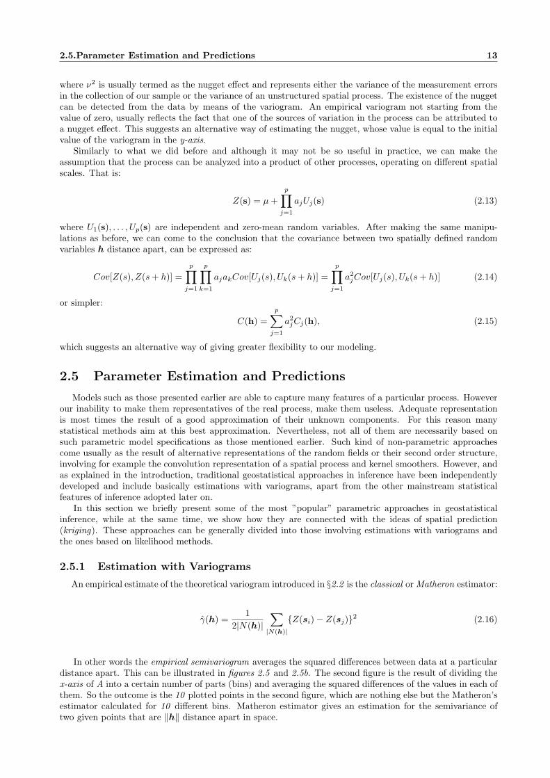
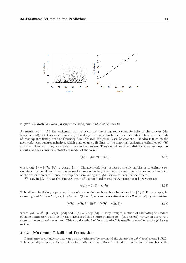
In other words the empirical semivariogram averages the squared differences between data at a particulardistance apart. This can be illustrated in figures 2.5 and 2.5b. The second figure is the result of dividing thex-axis of A into a certain number of parts (bins) and averaging the squared differences of the values in each ofthem. So the outcome is the 10 plotted points in the second figure, which are nothing else but the Matheron’sestimator calculated for 10 different bins. Matheron estimator gives an estimation for the semivariance oftwo given points that are ‖h‖ distance apart in space.

2.5.Parameter Estimation and Predictions 14

Figure 2.5 a&b: a Cloud , b Empirical variogram, and least squares fit.

As mentioned in §2.2 the variogram can be useful for describing some characteristics of the process (de-scriptive tool), but it also serves as a way of making inferences. Such inference methods are basically methodsof least squares fitting, such as Ordinary Least Squares, Weighted Least Squares etc. The idea is fixed on thegeometric least squares principle, which enables us to fit lines in the empirical variogram estimates of γ(h)and treat them as if they were data from another process. They do not make any distributional assumptionsabout and they consider a statistical model of the form:

γ(h) = γ(h,θ) + e(h), (2.17)

where γ(h,θ) = [γ(h1,θ1), . . . , γ(hn,θn)]′. The geometric least squares principle enables us to estimate pa-

rameters in a model describing the mean of a random vector, taking into account the variation and covariationof the vector elements. Hence the empirical semivariogram γ(h) serves as data for the process.

We saw in §2.3.1 that the semivariogram of a second order stationary process can be written as:

γ(h) = C(0)− C(h) (2.18)

This allows the fitting of parametric covariance models such as those introduced in §2.4.2. For example, byassuming that C(h) = C(0)·exp(−φh) and C(0) = σ2, we can make estimations for θ = {σ2, φ} by minimizing:

(γ(h)− γ(h,θ))′R(θ)−1(γ(h)− γ(h,θ)) (2.19)

where γ(h) = σ2 · [1 − exp(−φh)] and R(θ) = V ar[e(h)]. A very ”rough” method of estimating the valuesof these parameters could be by the selection of those corresponding to a (theoretical) variogram curve veryclose to the empirical variogram. This visual method of ”optimization” is usually referred to as the fit by eyemethod.

2.5.2 Maximum Likelihood Estimation

Parametric covariance models can be also estimated by means of the Maximum Likelihood method (ML).This is usually supported by gaussian distributional assumptions for the data. As estimates are chosen the

2.5.Parameter Estimation and Predictions 15

values of the parameters that maximize the logarithm of the n-variate gaussian pdf estimated at the observeddata:

L(θ; z1, . . . , zn) = −12ln{|Σ(θ)|}+ n · ln{2π}+ (Z(s)− 1µ)

′·Σ(θ)−1 · (Z(s)− 1µ)

Estimates with ML methods are not proved always to be so accurate in practice, especially when there aremany unknown parameters in our assumed model (i.e. nesting of many covariance models). The log-likelihoodcurve appears very often to be quite flat and this results into problems in the optimization methods. Thisis one of the main reasons why least square estimate methods applied to variograms are usually used asalternatives in geostatistics.

2.5.3 Predictions and Kriging

Geostatistical methods of prediction are typically known as methods of kriging. They are statistical toolshaving as a concern either the prediction of the response variable Z or a function of this response g(Z) at anunsampled location, say s ∈ <d. As in any other case of prediction, the interest of assessing the accuracy ofthese predictions is very frequent. One very common criterion for this assessment is the Square PredictionError :

{Zs − p(z; s)}2 (2.20)

where Zs is the true value of Z at the spatial location s while p(z; s) is the prediction at the same point,which is a function of the observed data z. Simpling kriging predictor is usually used as a predictor of zs, asit is the only among all the linear predictors of the form : p(z; s) = λ0 + λZ(s), that on average minimizes{Zs − p(z; s)}2 or equivalently the Mean Square Prediction Error : E{Zs − p(z; s)}2. This predictor is givenby the following relation:

p(z; s) = µz + σ2r′Σ−1

(z − µz

)(2.21)

and is usually referred to as the optimal least-squares predictor, as the values of λ0 and λ1 are the ones thatgive the solutions to this minimization problem.

In the case that the distributional assumptions of the random field are compatible with the ones of aGaussian process, the conditional mean of the process at the unsampled location s conditioned on all theother observed values, is given by:

E[Zs|z] = µz + σ2r′Σ−1

(z − µz

), (2.22)

which happens to be the simple kriging predictor. In this case the simple kriging predictor turns to be theBest Linear and Unbiased predictor under the mean square error criterion.

The reason is that the value of p(z; s) that generally minimizes E{Zs − p(z; s)}2 (best predictor) is equalto E[Zs|z]. This value turns out to be linear as well, as it is equal to simple kriging predictor in the gaussiancase (2.22). This is also an unbiased predictor as E[p(z; s)] = E

{E[Z(s0)|Z]

}= E[Z(s0)].

It is obvious from the above expressions that the simple kriging predictor is crucially reliant on theappropriate specification of the second order structure of the process under study.

Chapter 3

Models for spatio-temporalgeostatistical data

3.1 Introducing the New Dimension

It is many times the case that questions such as ”how much is something somewhere”, are not of thatinterest such as questions like ”how much is something somewhere and at time t”. Many processes, like forexample, meteorological or environmental, evolving not only in space but also in time as well, are on thedirect interest of scientists of the corresponding areas. It was not very late that spatio-temporal analysis ofprocesses became one of the main application areas of the geostatistical analysis, and at the same time thecomplementary tool of many sciences.

Although the joint analysis in space and time is based on the same principles such as the analysis in spatialfields, it has been practically proved that it hides many additional difficulties. Such difficulties do not arisefrom the fact that one more dimension has to be incorporated in our models, but from the recognition of thefact that space and time are two completely different physical notions. So, even though the spatiotemporaldomain of a process can be now expressed by <d×< and although this is mathematically equivalent to <d+1,physically this equivalence does not exist. Although, this does not impose any additional restrictions to thephilosophy of our analysis and the exploratory, inference and predictions techniques remain the same, the maindifficulties are related to the modeling of the second-order characteristics of the process. The fundamentalphysical difference between space and time needs to be acknowledged through the covariance function. Thisbrings us in front of the need of finding some most sophisticated expressions for such models. Unlikely withthe case of the purely spatial analysis, this time, very simple assumptions are quite often proved to be totallyunrealistic.

The greatest difficulty comes from the fact that as seen in §2.4.1, covariance functions (either in spatial orspatiotemporal) always need to satisfy certain conditions. On the contrary with the purely spatial case, suchkind of covariance functions are very rarely found for the needs of spatiotemporal modeling.

The main concern and the greatest challenge then becomes the finding of mathematical expressions ofspace-time dependence that are statistically valid. Thus, the basic restriction is neither statistical or compu-tational but has its origins in the ”world” of mathematics. The introduction of this new dimension opens anew field for further research in the geostatistical analysis.

In the text that follows, after referring to some alternative approaches for analysing spatio-temporal data,we make a small extension in the analysis of the previous chapter and do some adjustments in order to incorpo-rate time as well. We give some extra definitions relating to the construction of space-time covariance modelsand we perform some simulations. Aims of the simulations are two: 1) The better intuitive understandingof the newly introduced concepts and 2) the recognition of the over-simplicity of some common assumptionsand thus the emphasis for the adoption of a new methodology in space-time modeling. Finally, at the endof the chapter, we refer to some of some of the most popular and recent approaches in this area, which willserve as tools for the data analysis in Chapter 4.

3.2 Different Approaches in the Spatio-Temporal Analysis

The statistical analysis of the spatio-temporal random fields has been mainly visited by the following ap-proaches:

16

3.3.Nesting of Space-Time Covariance Functions 17

• Multivariate random field approach.

This methodology suggests the separate analysis of observations at different time instances. So, spatialvariability is modeled separately at different time periods. This approach is adopted mostly in the caseswhere data consists of a few number of temporal observations and when spatial predictions are requiredonly at a few time instances. An example for this is can be when the interest lies in the change of soilproperties after some treatment (ploughing harrowing). This for example can be gained by modelingthe temporal data, at the given locations, as a multivariate vector without making any assumptionsregarding temporal stationarity (Papritz & Fluhler 1994)

• Multivariate time-series approach

According to this approach, temporal analysis is performed separately for each spatial location. Thisis mostly preferable in the cases where the temporal observations are much more in number than thespatial ones, such as, for example, in the cases of modeling water fluxes in drain pipes. Stoffer (1986),for example, suggested the performanve of predictions only for the given temporal grid and the givenlocations. We also refer to Wikle and Cressie,(1999) and to Kyriakidhs & Journel (1999) for comparisonswith the previous approach.

• Spatial parameter field approach

For example, Extreme value field, where the parameters of the marginal distribution at each site aregiven by stationary Gaussian random field, such as Casson’s and Coles’s (1999) approach in extrememeteorological events.

• Geostatistical Approach:

This is the approach that we adopt here , that is the spatio-temporal data analysis with methods forrandom fields in Rd+1 and the modeling of joint spatial and temporal variability. Examples of this canbe the modeling of soil’s temperature or its moisture over time.

Joint analyses of spatio-temporal data are preferable to separate analyses. Nevertheless, in the process ofbuilding a joint model, separate analyses are very often proved to be quite valuable tools. The modeling ofthe dependency structure of the spatiotemporal random field, just as in the purely spatial case, can be carriedout either in the observation or in the frequency domain.

3.3 Nesting of Space-Time Covariance Functions

We saw in the previous chapter the possibility of constructing covariance functions through nesting ofsimple covariance functions, either expressed as their sum or their product. This can be usually thought of asa representation of a process composed by different sources of variations and from a mathematical perspectiveas a straightforward way of giving flexibility to our covariance model. We will use the same results and wewill generalize them by incorporating time as an extra dimension: In particular, by using (2.7) from section2.4.4 , we derive:

Z(s, t) = µ+p∑

j=1

ajUj(s, t), (s, t) ∈ <d ×<

where U1(s, u), . . . , Up(s, u) are independent and zero-mean random variables. In general that means thatCov(Uk(si, u), Uk+ν(sj , u)) 6= 0 ∀ k, i, j in [1, p], only if ν = 0. Furthermore, the covariance function of Z canbe expressed as:

Cov[Z(s, h), Z(s+ h, t+ u)

]=

p∑j=1

a2jCj(s, t,h, u), where Cj(s, t,h, u) = Cov[Uj(s, t), Uj(s+ h, u)]

Working similarly as before, the generalization in the case of products is:

Z(s, t) = µ+p∏

j=1

ajUj(s, t)

3.4.Separable Space-Time Models 18

While for the covariance holds respectively:

Cov[Z(s, h), Z(s+ h, t+ u)

]=

p∏j=1

a2jCj(s, t,h, u), where Cj(s, t,h, u) = Cov[Uj(s, u), Uj(s+ h, u)]

Example

Consider now the particular case where p = 2, U1(s, t) = U1(s) and U2(s, t) = U1(t). The random fieldcan be expressed as:

Z(s, t) = U1(s) + U2(t) and Z(s, t) = U1(s)× U2(t)

That is, the sum and the product of a purely spatial and purely temporal independent random fields. Thecovariance functions that are produced are:

Cov[Z(s, t), Z(s+h, t+u)

]= C1(s,h)+C2(t, u) and Cov

[Z(s, t), Z(s+h, t+u)

]= C1(s,h)×C2(t, u)

(3.1)This is a particular case of the ”famous” class of separable spatio-temporal covariance functions. Although inthis case the random field is constructed by two random processes existing in space and time independently,the definition of separability has to do with the mathematical expression of the covariance function.

3.4 Separable Space-Time Models

Separability is defined to be the case when the mathematical expression of covariance function impliesno interaction between the spatial and temporal components. The example given above gave us an intuitiveinterpretation of what that practically means. Of course this interpretation would be more difficult in the casethat the covariance function is composed by many sums and products of various purely spatial and temporalcovariance functions. As in practice one reason of being used is their computational tractability , separabilityis often defined to be the cases where the spatio-temporal covariance function can be expressed as (3.1) .Separable space-time models is the simplest class of spatial-temporal covariance functions and suggest a veryeasy way of producing valid covariance functions (property in 2.4.1) and at the same time acknowledging thephysical difference between space and time.

3.4.1 Some Examples of separable models

For convenience in the notation, from now and on: C(s, t;h, u) = Cov(Z(s, t), Z(s+ h, t+ u)).

1. Simple caseC(s, t;h, u) = σ2

1 · exp(−φ1 · ‖h‖) + σ22 · exp(−φ2 · ‖h‖)

The components have usually different parameters to allow for space-time anisotropy

2. Combination of purely space covariance functions

C(s, t;h, u) = σ2 · exp(−φ1 · ‖h‖) · gauss(h;φ2) +mattern(u;φ3)

In this case the spatial covariance component: C1(s, s+h) = cA1(s, s+h) ·cB1(s, s+h), is the productof two others sub-components.

3. Extra nugget term

C(s, t;h, u) = σ2 · exp(−φ1 · ‖h‖+ φ2 · u) + ν2 · gauss(φ3;u)

Here the ”extra” part ν2 · gauss(φ3;u) can be thought of as a spatial nugget which depends on time.In the special case, when φ3 is 0, the last component reduces to the simpler case where nugget isindependent in space and time.

Note that: σ2 · exp(−φ1 · ‖h‖+ φ2 · u) = σ21 · exp(−φ1 · ‖h‖) · σ2

2 · exp(−φ2 · u).

3.5.Non-Separable Models 19

3.5 Non-Separable Models

Despite its advantages, one main disadvantage of the previous class of models is that it does not allow theincorporation of space-time interactions. Every spatio-temporal covariance function that cannot be simplifiedinto a sum or product of a purely spatial and temporal covariance function, it belongs into the non-separableclass of spatio-temporal covariance functions. We can think of this category as the most general, wherespace-time interactions are allowed.

3.6 Stationary Space-Time Models

No matter whether separable or not, by extending our definitions of the previous chapter, we define thespace-time covariance function to be strictly stationary if: when the joint distribution of any spatiootemporaldefined random vector {Z(s1, t1), . . . , Z(sn, tn)} is the same with the joint distribution of {Z(s1 + h, t1 +τ), . . . , Z(sn + h, tn + τ)}, for any h, τ ∈ <d ×< and n ∈ Z.

Similarly the spatiotemporal random field has weakly or second order stationary covariance function if:it has a spatially stationary covariance, that is C(s, t;h, u) = C(t;h, u) and a temporally stationary one:C(s, t;h, u) = C(s, t;h), which implies that C(s, t;h, u) = C(h, u). As before, the second-order stationarityrequires constant mean E[Z(s)] = µ.

In practice it is difficult to work with a non-stationary (second order) spatio-temporal covariance function.Just as described in the previous chapter, frequently trend removal and space deformation techniques (Haslettand Raftery 1989; Sampson and Guttrp 1992) are needed to allow for a reduction to a stationary covariancefunction.

3.7 Anisotropy?

Although isotropy is well defined in space there is no point to talk about anisotropy in time, as it isan one-dimensional measure. For this reason we can divide the space time covariance function into two-categories: Spatio-isotropic and Spatio-anisotropic. However, when we consider space and time together wecan observe patterns in the space-time correlation structure that lack of symmetry. Consider for example theone dimensional space case when we measure the quality of water of a river in two points (A and B) thatare about 1km far apart. By considering that the water flows from A to B, it is plausible to assume that thequality of the water in A now (At) resembles more with the quality of water at B after 5 minutes (Bt+5),compared to how Bt (the quality of water in B now) resembles to At+5 (the quality of water in A after 5minutes) . The patterns observed in the dependence structure may resemble a lot to the ones observed in thetwo-dimensional space geometrical-anisotropy paradigm. However, this in geostatistical space-time literaturethis is termed as lack of fully symmetry.

3.8 Fully-Symmetry

Whether being separable or not and independently from if it is stationary, Gneiting (2002) defines therandom field Z(s, t) to have fully symmetric covariance if:

cov{Z(s, t), Z(s+ h, t+ u)} = cov{Z(s, t+ u), Z(s+ h, t)}, ∀(s,h), (t, u) ∈ <d ×<

All the separable models are fully-symmetric. To give an explanation for this, consider the most ”popular”case of separable space-time covariance functions, where:

Cov{Z(s, t), Z(s+ h, t+ u)

}= C1(s,h)× C2(t, u) (3.2)

Consider now the spatially and temporally defined random variables: Z(s, t + u) and Z(s + h, t). Theircovariance is given by:

Cov{Z(s, t+ u), Z(s+ h, t)

}= C1(s,h)× C2(t, u) (3.3)

3.8.Fully-Symmetry 20

From the previous equations it follows that:

Cov{Z(s, t), Z(s+ h, t+ u)

}= Cov

{Z(s, t+ u), Z(s+ h, t)

}(3.4)

which is the definition of fully-symmetry. Although separability implies fully symmetry, the inverse is not true.This suggests a method of making a test for Separability. By rejecting the fact that the random field is fullysymmetric, we rejecting also the possibility for being separable (Scassia & Martin 2005; Lu & Zimmerman2005)

3.8.1 Not Fully-Symmetric Space-Time Covariance Models

In the example with the river we showed that working always under fully symmetry cannot always be arealistic assumption. Its very often the case when atmospheric, environmental and geophysical processes areunder the influence of prevailing air or water flows, resulting in a lack of full symmetry. Transport effects ofthis type are well known in the meteorological and hydrological literature (see for example Gneiting (2002a);Stein 2005; Luna & Getton 2005; Huang & Hsu 2004).

Various approaches have been taken in order to encompass this characteristic to the covariance structureof the space-time random field. If a space-time process involves dynamic physical processes, the stationarycovariance function might depend on for example on the space-time lag through a distance function of theform ‖h − V u‖, where V is a velocity vector in <d. We give just an idea by considering the Lagrangiancovariance proposed by Cox & Isham (1988), as a physical model for rainfall, which can be generally thoughtof as being attached to and moving with the center of an air or water mass. Cox & Isham showed in particularthat if V is a random vector in <2 and G(r) denotes the area of intersection of two disks of common unitradius whose centers are a distance r apart, then

C(h, u) = E{G(h− V u)

}, (h;u) ∈ <d×< (3.5)

is a valid space-time covariance function. (Note that the expectation is taken with respect to random vectorV ). Lagrangian covariance structures have indeed been discussed in meteorological and hydrological literature(see for example Boutlier (1993); Desroziers & Lafore (1993); May & Julen (1998)). Stationary space-timecovariance functions that are not fully symmetric can also be constructed on the basis of diffusion equationsor stochastic partial differential equations. We refer to Jones & Zhang (1997), Christakos (2002), Brown,Karesen, Roberts & Tonellato (2000), Kovolos, Christakos, Hristopoulos & Serre(2004), Stein (2004).

Research along these lines is currently under development, and well-founded strategies for spatiotemporalmodeling remain in great demand.

3.9.Simulations of Simple Spatio-Temporal Gaussian Random Fields with DifferentDependency Features 21

Figure 3.8: Classes of space-time covariance functions

3.9 Simulations of Simple Spatio-Temporal Gaussian Random Fieldswith Different Dependency Features

In this section we perform simulations of various spatio-temporal Random Fields with different character-istics in the covariance function. It was always a common belief that simulating from a particular model isone of the best ways to understand it. Our here, aim is trying to give a good idea of the practical meaning ofthe previously defined concepts.

In the previous chapter we examined the reasons why the Gaussian Random Field (GRF ) holds a coreposition in geostatistical analysis. We remind that one of them was the fact that it is fully characterized byits mean and its variance. This implies that by specifying a mean and covariance structure we can adequatelysimulate from it. On the contrary, it is usually impossible to construct a realization from a non-gaussianspatial distribution via simulation from it. The multivariate gaussian pdf is given by:

f(Z(s, t)) =1

|Σ| 12· 1(2π)

n2exp{− 1

2(Z(s, t)

)T Σ−1(Z(s, t))}, (3.6)

where in our case: Z(s, t) = [Z(s1, t1), . . . , Z(sn, tn)]′.

Many methods are available to simulate GRF’s. However this is not always easy as it depends what exactlywe are interested in to simulate. Many difficulties for example arise in some particular cases, as for examplein the case that simulation should be made into a non-irregular grid of many locations or when the covariancestructure is quite complex. For this reason many methods have been suggested such as circular embedding,turning bands and methods based on Fourier series to name a few. But as said in the beginning, purpose ofthis section is not examining alternative ways of simulation but to give a better intuitive understanding ofthe previously introduced notions regarding the various spatio-temporal second-order characteristics.

All the simulations are performed in one dimensional space, as such an illustration would be impossible toa greater number of spatial dimensions. Moreover, all of them are performed under second-order stationarity

3.9.Simulations of Simple Spatio-Temporal Gaussian Random Fields with DifferentDependency Features 22

assumptions and for matters of simplicity we used the exponential correlation function. It should be notedthat the word ”simple” in the title of this section has mostly the meaning of ”theoretical” as reality is alwayscomplex. But this is something that will be further discussed and analyzed in the next section.

Preliminaries

In order to perform space-time asymmetric simulations we should make use of a matrices that linearly trans-form the space-time coordinate system. Practically, the same matrices were used for simulating anisotropicrandom fields in space. Their physical interpretation in the space-time case, though, is totally different forreasons explained earlier regarding the fact that there is no anisotropy in time. So, the same mathematicaltools are used and enable us to simulate spatio-temporal random fields with various characteristics in thecovariance structure. In particular, we are making use of the following space-time transformation matrix:

Ai =[αixx

αiTx

αixT

αiTT

]where αixx and αiTT are the scale parameters for space and time respectively, while αixT and αiTx can be

seen as the parameters giving symmetric ”shape” to the random field.It should be noted that this particular method enables us simulating only particular cases of not symmet-

ric space-time models, as it is not always the case that non-symmetric space-time coordinate system can becorrected by a linear transformation.

All the examples given are particular cases of the following covariance scheme:

C(d) =N1∑i=1

Ci(‖d ·Ai‖) +N2∏j=1

Cj(‖d ·Aj‖) (3.7)

which are the entries of the n × n covariance matrix Σ (equation 3.6) and represent the strength of rela-tionship between spatially and temporally defined random variables, with separation described by the 1 × 2vector d = [h, u], where h and u ∈ <1, Ci(‖d ·Ai‖) = exp(−‖d ·A1‖) and N1, N2 ≤ 2. The simulations wereperformed with the use of the R software package: ”RandomFields version 1.3.28”.

3.9.1 Simulating a Random Field with a Non-Separable and Fully SymmetricCovariance Function

In this first example we provide interaction between the spatial and temporal components (as non-separabilityimplies) by trying to incorporate them into one covariance function. So, in this case N1 = 1 and N2 = 0 (seeeq. 3.7 ) and we define the covariance function to be fully symmetric by setting the non-diagonal elements tobe different from zero:

A1 =[α1xx

00

α1TT

], which produces :

CA(d) = exp(−‖d ·A1‖) = exp(−√

(a1xx · h)2 + (a1TT · u)2), where a1xx = 6, a1TT = 0.7

The result is illustrated in figure 3.9a. We set a1xx 6= a1TT to emphasize the physical distinction betweenspace and time: The rate of dependence between random variables 1 space unit apart is usually differentbetween the dependence between random variables 1 time unit apart, as this units are not comparable.

It should be observed that the square root does not allow the simplification of this expression into aproduct of two exponential covariance functions (a purely spatial and a purely temporal one), and so space-time interaction is allowed.

3.9.Simulations of Simple Spatio-Temporal Gaussian Random Fields with DifferentDependency Features 23

3.9.2 Simulating a Random Field with a Non-Separable and Not Fully-SymmetricCovariance Function

Here we do exactly the same with the only difference that the non diagonal elements of A are non-zero:

N1 = 1, N2 = 0, A1 =[α1xx

α1Tx

α1xT

α1TT

]This results into the following covariance specification:

CB(d) = exp(−‖d ·A1‖) = exp(−√

(a1xx · h+ a1Tx · u)2 + (a1TT ·∆T + a1xT ·∆x)2)

As before, the spatio-temporal dependence cannot be separated to a purely spatial and temporal part respec-tively. We set a1xx = 6, a1TT = 0.7, a1Tx = −4 and a1xT = −4, and we depict the result into the secondpart of figure 3.9 .

2 4 6 8 10

24

68

10

Space lag ||h||

Tim

e la

g |u

|

2 4 6 8 10

24

68

10

Space lag ||h||

Tim

e la

g |u

|

Figure 3.9, a and b: Simulation of a random field with a a fully-symmetric and b a non fully-symmetric,covariance functions (stationary and non-separable)

3.9.3 Simulating two Random Fields with a Separable Dependency Structure

Separable covariance function means no interaction between spatial and temporal components. Thus oneeasy way of doing that is to specify two separate covariance functions, one for space and one for time re-spectively. In the case of space this can be achieved by setting all the time components of the matrix A:aTT , aTx, axT equal to zero. The physical interpretation of aTT = 0 is that the the spatio-temporal randomvariables that are u apart in space are independent. And likewise, when specifying a purely temporal covari-ance function we set all the space components axx, axT , aTx to be zero, as well, where axx = 0 means that thethe spatio-temporal random variables that are h apart in space are independent.

N1 = 0, N2 = 2, A1 =[α1xx

000

],A2 =

[00

0α2TT

]

CC(d) = exp(−‖d ·A1‖) · exp(−‖d ·A2‖) = exp(−|a1xxh|) · exp(−|a2TTu|)

By setting the parameters a1xx = 4 and a2TT = 2, the realization is illustrated in figure 3.91aWe proved earlier that separability implies fully-symmetry and we said that the inverse does not hold. In

our case we can practically validate this as well , by setting any of the non-diagonal elements of A1 or A2 (orboth) to be different from zero (loss of fully-symmetry). What we are going to observe is a similar pattern tothe figure 3.9b, while in the mathematical part what we are going to have is an interaction between the spaceand time components, which implies non-separability.

Finally, we simulate a spatio-temporal random field that has separable covariance structure which is a sumof a purely spatial and a purely temporal covariance functions.

3.10.Realism vs. Convenience 24

N1 = 2, N2 = 0, A1 =[α1xx

000

],A2 =

[00

0α2TT

]

CD(d) = exp(−‖d ·A1‖) + exp(−‖d ·A2‖) = exp(−|a1xxh|) + exp(−|a2TTu|)

For the same a1xx and a2TT , the result is shown in figure 3.91b.

2 4 6 8 10

24

68

10

Space lag ||h||

Tim

e la

g |u

|

2 4 6 8 10

24

68

10

Space lag ||h||

Tim

e la

g |u

|

Figure 3.91, a and b: Simulation of two random fields with two different kinds of separable Covariancefunctions

3.10 Realism vs. Convenience

As emphasized in the beginning, purpose of the previous examples was to give a better understanding of thedistinction between different characterizations regarding the covariance function. However, in practice suchprocesses are not observable and we will justify this in the rest of the chapter. What follows is a discussionabout the advantages and disadvantages of separable and non-separable space-time covariance models.

Advantages and Disadvantages of Separable Covariance functions

Advantages

• Guarantees the Validity of the Covariance Function. Separable covariance models provide withan easy and convenient way of producing valid covariance functions, by multiplying or adding a spatialand a purely temporal covariance function. (property in §2.4.1) . In the simulations before, we chosethe simplest possible examples of a separable model: exp(−‖d ·A1‖)× exp(−‖d ·A2‖): two exponentialfunctions one for space and one for time. Although this is not so realistic, we could have easily chosenany other two valid covariance functions, one for space and one for time.

• Computational Convenience. Consider for example the spatio-temporal random vector: Z(s, t) ={Z(s1, t1), . . . , Z(sn, tn)},s, t ∈ <d ×<, with separable covariance function given by:

cov(Z(si, ti), Z(sj , tj)) = σ2C1(si − sj ;φ) · C2(ti − tj ;ψ) (3.8)

The fact that we have a separable covariance model, allows us to write the covariance matrix of Z(s, t)as a product of two other submatrices:

ΣY (σ2,φ,ψ) = σ2ΣS(φ)⊗ΣT (ψ) (3.9)

where ΣS is an I × I covariance matrix with elements C1(si − sj ;φ), and ΣT is an I × I covariancematrix with elements C1(si − sj ;φ). As long as C1 and C2 are positive definite, the covariance matrix

3.10.Realism vs. Convenience 25

of Z is positive definite as well. The Kronecker product form of (3.9), provides many computationalbenefits. For example consider the likelihood of Z:

−12· |σ2ΣS(φ)⊗ΣT (ψ)| − 1

2σ2(Z − µ)

′(σ2ΣS(φ)⊗ΣT (ψ))−1(Z − µ)

but, this computation becomes more tractable due to the two properties:

|σ2ΣS(φ)⊗ΣT (ψ)| = (σ2)IJ |ΣS(φ)|J⊗|ΣT (ψ)|I and (σ2ΣS(φ)⊗ΣT (ψ))−1 = ΣS(φ)−1⊗Σt(ψ)−1

Disadvantages

• No space-time interactions. Even if we had found the most suitable covariance functions for thepurely spatial and the purely temporal processes, the fact that spatial and temporal lag componentsdon’t interact, is the strongest reason why someone would not want to work with these models. It seemsquite unrealistic to assume that the random field is composed by two random processes existing in thespatial and temporal domains independently (see §3.3).

Certain configurations of covariance functions of the form C1 + C2 (such as the second simulation in§3.9.3) make Σ to be singular.

Advantages and Disadvantages of Non-Separable Covariance functions

Advantages

• Space-Time Interactions. According to what said before, the greatest reason that someone prefers towork under non-separability assumptions is the incorporation of space time interactions, which meansthat the spatio-temporal random field is treated as a single random process ”living” together in spaceand time.

Disadvantages

• Not Necessarily Tractable. We saw earlier why the separable covariance models are in general morecomputationally convenient than non-separable ones. However, the degree of difficulty always dependsevery time on the particular case of non-separable function.

• Matters of Validitity and Mathematical Restrictions

In our first simulation-example given above (non-separable and fully-symmetric covariance) we veryeasily managed to incorporate both space and time into a single exponential covariance model: exp

(−√

(a1xx · h)2 + (a1TT · u)2). Although space and time are allowed to interact, the main problem is that

such an expression does not acknowledge any physical difference between them. The way of dependencyin time is considered to be similar just as the way of dependency in space, which means that the formeris practically treated just as an extra dimension in space. Such kind of non-separable models are usuallyreferred to as models based on space-time metrics (Gneiting & Schlather 2002) and are of the generalform: C(h;u) = φ(ασ‖h‖2 + ατu

2), (h, u) ∈ <d × <. Although this is only a very particular case ofthe general non-separable class of models, there is a great lack of such models that are able to capturethe difference in the actual and different behavior between space and time. The reason is related withthe practical difficulty for someone to specify a covariance model that acknowledges this difference,incorporates space and times interactions, while at the same time is valid §2.4.1. So, one of the reasonsfor providing this example besides simplicity, could be also the scarcity in the variety of non-separablemodels.

It can be concluded then, that the greatest disadvantage of these kind of functions is mostly related withour mathematical difficulty in producing valid covariance functions that are able to recognize space andtime as two non comparable measures.

The ability of the construction of valid space-time covariance functions is one of the main challenges inthe geostatistical modeling of spatio-temporal processes. Many times, things become even more difficult whenother characteristics of the process need to be incorporated, such as in cases where there is a lack of fullysymmetry.

The most popular of the approaches that have been taken, are based on Fourier integral analysis and inBochner ’s theorem (§2.4.3).

3.11.The Creesie-Huang Approach 26

3.11 The Creesie-Huang Approach

We saw in the previous chapter (§2.4.3) that the only way to ensure that a covariance function is positivedefinite is to be able to express it through a Fourier integral.

C(h) =∫ ∫

exp{ih′ω}g(ω)dω , (3.10)

where F is a finite no-negative and symmetric measure on <d×<. Furthermore, Bochner (1955) showed thatevery matrix is positive definite if and only if it can be expressed as (3.10). By incorporating time as an extradimension, this becomes:

C(h;u) =∫ ∫

exp{ih′ω + iuτ}g(ω; τ)dω dτ (3.11)

As in the purely spatial case, this expression enables someone to construct a valid space-time covariancefunction by just specifying a joint spatio-temporal spectral density g(ω; τ). Creesie & Huang (1999) provideda clever device in which the selection of such a function is avoided and thus introduced classes of non-separable, stationary covariance functions that allow for-space time interactions. Specifically what they didwas to express g(ω; τ) as:

g(ω; τ) = (2π)−1

∫exp(−iuτ)h(ω;u)du, where h(ω; τ) = (2π)−d

∫exp(−ih

′ω)C(h;u)du (3.12)

is the spatial spectral density function. Then by substituting it in (3.11):

C(h, u) =∫ ∫

exp{ih′ω + iuτ}

[(2π)−1

∫exp(−iuτ)h(ω;u)du

]dω dτ =

∫exp(ih

′ω)h(ω;u)dω (3.13)

So, they managed to express the spatio-temporal covariance function as one dimensional fourier transformof a h(ω;u). The advantage of this method is that by specifying the spatial spectral density h(ω;u) we canconstruct a spatio-temporal covariance model C(h, u). This is much easier than in the case that we had tospecify directly the joint spatio-temporal density g(ω; τ). Furthermore, they tried to express h(ω;u) as aproduct of two other functions ρ(ω;u) and k(ω) as a means of making the integration in (3.13) easier.

3.12 Gneiting’s Family of Non-Separable Models

Creesie and Huang’s approach was novel and powerful, but depends on Fourier transform pairs in <d. Inother words it is restricted to a comparably small class of functions, for which a closed form solution to thed -variate Fourier integral is known. Gneiting(2002a) presented a flexible and elegant approach to constructspatio-temporal covariance functions. His method was powerful because it does not require operations in thespectral domain and builds valid covariance functions from elementary components whose validity is easilychecked. In particular let φ(t), t ≥ 0 be any completely monotone function and ψ(t), t ≥ 0 be any positivefunction with a completely monotone derivative. Then:

C(h, u) =σ2

ψ(u2)d/2· φ

(‖h‖2

ψ(|u|2)

)(3.14)

is a valid space-time covariance function on <d ×<.Gneiting provided thus very general classes of models that does not depend on the closed form Fourier

inversion and does not require integrability. Its should be noted that even though these models are non-separable in general, each of their components, φ(t) and ψ(t), can be associated with the data’s spatial andtemporal structures respectively. In his paper, Gneiting provides a table with a range of possible choices ofsuch a functions. Many of them all illustrated in Table 1 below:

A Some Completely Monotone Functions φ(t), t ≥ 0 B Some Positive Functions ψ(t), t ≥ 0φ(t) = exp(−ctγ), c > 0, 0 < γ ≤ 1 ψ(t) = exp(atα + 1)β , a > 0, 0 < α ≤ 1, 0 ≤ β ≤ 1φ(t) = (1 + ctγ)ν , c > 0, 0 < γ ≤ 1, ν ≥ 0 ψ(t) = ln(atα + b)/ln(b), a > 0, β > 1, 0 < α ≤ 1φ(t) = (2ν−1Γ(ν))(ct

ν2 )Kν(ct

ν2 ), c > 0, ν ≥ 0 ψ(t) = (atα + b)/(b(at + 1)), a > 0, 0 < β ≤ 1, 0 < α ≤ 1

3.12.Gneiting’s Family of Non-Separable Models 27

Table 1 Examples of A. Completely monotone and B. Positive definite functions.

Example:

Consider the first two entries of the two columns of the previous table:

φ(t) = exp(−ctγ) and ψ(t) = exp(atα + 1)β

By substituting them into (3.14) we get:

C(h, u) =σ2

(atα + 1)βd2

· exp{ c‖h‖2γ

(atα + 1)βγ

}(3.15)

Note that for β = 0 the covariance does not depend on the time lag. Multiplying (3.15) by a purely temporalcovariance function: 1

(atα+1)δ , this becomes:

C(h, u) =σ2

(atα + 1)δ+ βd2

· exp{ c‖h‖2γ

(atα + 1)βγ

}, (3.16)

where for β = 0 now reduces into a separable covariance function. This suggests a way of testing theseparability assumption.

Gneiting showed that some of the covariance functions in the paper of Creesie and Huang were notvalid, because one of their correlation functions used in their examples did not satisfy the needed conditions.Note that Gneiting’s class of models are stationary and fully symmetric and his method of producing validcovariance functions is sometimes referred to as a monotone function approach.

While these methods of constructing valid covariance functions were based on fourier analysis, otherpossible methods for constructing such models can include the mixture approach (for example Ma 2002) orthe differential equation approach (see Jones & Zhang 1997).

Chapter 4

Case Study: Spatio-TemporalModeling of the Portuguese FishStocks

4.1 Introduction

The objective of the previous chapter was to present the difficulties arising in the modeling of a space-timeprocess and give some ideas of how these problems are able to be solved. We saw that many models havebeen suggested and many of the restrictions were overcome by the construction of complex mathematicalexpressions.

Although some models look more attractive than the others, this does not mean that they are more usefulin practice. The adequacy of a particular class of models can only be assessed by being practically tested toa particular problem and under all the possible circumstances that can occur. This automatically implies asoftware implementation for this kind of models and at the same time its assessment to a number of differentapplication areas.

Unfortunately an additional restriction in the development of space-time modeling comes from the fact thatthere is a great lack in their support by statistical software programs. Another remarkable fact is that mosttimes their applicability lies mostly on areas where the most practical interest is focused, such as meteorology,hydrology, atmospheric environmental or geophysical sciences etc.

In this last chapter of this project, our aim is to make a big step toward these two kind of limitations.In particular we use one of the most recent packages in order to assess the suitability of a particular class ofmodels to an application area not often visited by statisticians. Being motivated by the last section of theprevious chapter, we test how the Gneiting ’s class of non-separable models corresponds to the monitoring ofthe fish stock of the Portuguese coast during the period of the years 1990-2004. We build a model based onthe data not including the last year of observations and thus are able to assess the quality of our one yearforward predictions. This will enable us to test their ability to cover the inadequacies resulting from the useof a simple separable space-time model and thus discussing if it worths losing some simplicity to give morerealism to our model. Furthermore, we make some discussions regarding the difficulties involving inferencefor this particular family of models.

4.2 Scientific Interest and Data Description

Our data consist of information regarding the fish stock in the Portuguese coast over the period of years1990-2004. Purpose was the monitoring of fish stock in this particular area. Knowing the behavior of fishstock and its evolution in time, is quite important for decisions regarding the annual permissible fishing quotasthat guarantee the perpetuation of the fish species and at the same time the sustainable development of thearea. Annual information about the stock of various kind of fish was collected by means of a big net thrownfrom a boat in a set of 57 particular locations in the sea around the Portoguese coast. Although samplesfrom various kind of fish were collected, our interest is going to be focused on information regarding ”hake”,

28

4.3.The Need for Joint Space-Time Analysis 29

as this species is found to exist almost everywhere in this area and is thus more suitable for geostatisticalanalysis. Our data-sample then consists of 57 annually collected observations, constituting thus a total setof 57 × 15 = 855 spatio-temporal defined observations. Figure 4.2 below , illustrates the spatial samplinglocations and the Portuguese coast boundaries.

−9 −8 −7 −6 −5 −4

3738

3940

4142

Longitude

Latit

ude

●

●●

●

●

●

●

●●●

●●

●

●●

●

●

●

●

●

●●

●●

●●

●

●

●

●

●● ●●

●●

●

●●

●●

●●●

●

●

●

●

●●

● ●●

●

●●

●

Figure 4.2: Map of the sampling locations and the Portuguese coast. The dotted lines represent the seadepth contours.

4.3 The Need for Joint Space-Time Analysis

Whether the average fishing quota or the one collected in the particular locations increases or decreasesis one of the main interests of the survey. Obviously, the interest is not restricted in the fish stock in these57 locations but also in the one existing everywhere in this area. Unfortunately, the very high cost of takingsamples from the whole region makes the need for investigating other kinds of solutions quite essential. Froma geostatistical point of view, the spatial distribution of fish stock at a particular time point, can be viewed asa stochastic process characterised by some geostatistical parameters, the most important of which synthesisesthe continuity structure derived from the data. This probabilistic framework allows us to analyse and quantifythe uncertainty characterising the spatial distribution of the fish stocks and furthermore, enables us makinginterpolations into all the unsampled locations. However, although this seems to be a quite good solution, wewaste any information coming from the samples taken from the previous years.

An additional interest may be the prediction of the fish stocks in the next years. What we can easily thinkin this case, is just to perform a time-series analysis for each of the 57 locations in order to be able to performpredictions in future time points. Such as in the previous case , although this seems to be a quite goodsolution, we waste information coming from the samples taken from other points in space. Another problemis that 15 time points are not an adequate sample for such kind of analysis , which allows for predictions onlyon the sampled time-points.

The quality of our analysis can be much improved by considering the whole data as a single realizationfrom a space-time stochastic mechanism and performing a joint space-time analysis. This mechanism will beable to describe not only how the spatial variables are associated with each other but also how the wholesystem of spatial and temporal defined variables behaves.

4.4 Methods

The fact that a joint spatio-temporal analysis proves to be better than the purely spatial analysis overdifferent time periods, is something that cannot be generalised in all the cases. Very often, problems such asfor example, the absence of temporal correlation or the instability of the purely spatial properties over timedo not allow for the construction of a space-time model. This is something that was taken into account in our

4.5.Exploratory Data Analysis and Assumptions 30

analysis and for this reason various kinds of tests were performed with the purpose of reinforcing the validityof our final space-time analysis.

More specifically, the methodology followed in the modeling of the Portuguese fish stocks was the following:Initially, we perform a purely spatial analysis over the 14 time periods in order to investigate the stability of thespatial process’ properties over time. This is further checked by the fitting of a purely spatial model assumingconstant properties over time and its comparison with the previous one. Given that the spatial process hassimilar characteristics over time, we check whether a spatiotemporal model with separable covariance function,is able to provide a better fit under the same second-order assumptions in space. This is something that tests,at the same time, the evidence of temporal correlation, as the small number of observations in time doesnot allow for the adequate inspection of the temporal properties alone. Finally, if this last simple separablespace-time covariance model proves to be more suitable than the model assuming the absence of temporalcorrelation, we check whether the specification of a more general, Gneiting’s type non-Separable covariancemodel is more adequate for our data. Synoptically, our data analysis involves the testing of the following foursuccessive hypothesis:

• H0: Spatial process with the same properties over time. (or spatio-temporal process with the absenceof temporal correlation!)

• H1: Spatial process with different properties over time.

• H2: Spatio-temporal process with separable covariance function.

• H3: Spatio-temporal process with non-separable covariance function, of Gneiting ’s type.

The hypothesis testing procedure in the analysis can be represented by the following scheme:

Testing H0 against H2 is pointless in the case where H0 is rejected against H1. In the same manner thehypothesis testing of H2 against H3 requires the rejection of H0 against H2. In each case, the acceptance orrejection of Hν , will be supported by exploratory tools such as variograms and by more formal methods suchas likelihood ratio tests and assessment of predictions.

4.5 Exploratory Data Analysis and Assumptions

Distribution of the Data

The marginal distribution of the data sample appeared to be highly skewed and thus not in an agreementwith that of a normally distributed random variable. This can be illustrated by the histogram of the data, inthe first part of the next figure below. However, a Box-Cox transformation with λ = 0.25, gave a satisfactoryapproximation:

z∗ =z0.25 − 1

0.25(4.1)

The histogram and the QQ-plot of the transformed sample is illustrated in the second and third part of figure4.5.

4.5.Exploratory Data Analysis and Assumptions 31

Transformed Variable

Fre

quen

cy

0 1000 2000 3000 4000

020

040

060

080

0

Transformed Variable

Fre

quen

cy

−5 0 5 10 15 20 25 30

050

100

150

200

250

●●

●

●

●

● ●

●

●

●

●

●

●

●

●

●

●

●

●

●

●

●

●

●●

●

●

●

●

●

●

●

●

●

●

●

●

●

●

●

●●

●

●

●

●

●

●

●

●

●

●

●

●

●

●

●

●

●

●

●

●

●

●

●

●

●

●

●

●

●

●

●

●

●

●

●

●

●

●

●

●

●

●

●

●

●

●

●●

●

●

●

●

●

●

●

●

●

●

●

●

●

●

●

●

●

●

●

●

●

●

●

●

●

●

●

●

●

●●

●●

●

●

●

●

●

●

●

●

●

●

●

●

●

●

●●

●

●●

●●

●

●

●

●

●

●

●●

●

●

●

●

●

●

●

●

●●

●

●

●

●

●

●

●

●

●

●

●

●

●

●

●●●

●●

●

●

●

●

●

●

●●

●●

●●

●

●

●

●●●

●●

●

●●

●

●

●

●

●●●

●

●

●

●

●

●

●

●

●●

●

●

●●

●

●

●

●

●

●

●

●●

●●

●

●

●

●

●

●

●

●●

●

●

●

●

●

●

●●

●

●

●

●

●

●

●

●

●

●

●

●

●

●●

●

●

●

●

●

●

●

●

●

●

●

●

●

●

●

●

●

●

●

●

●

●

●●

●●

●

●

●

●

●

●

●

●

●

●

●

●

●

●

●●

●

●

●

●

●

●

●●

●

●

●

●

●

●

●

●

●

●

●

●

●

●

●

●

●●

●

●

●

●

●

●

●

●

●

●

●

●

●

●

●●

●●

●

●

●●

●

●

●

●

●

●

●

●●

●●●

●●

●

●

●

●

●●●

●

●

●

●

●●

●

●●

●

●●●

●

●

●

●

●

●

●

●

●

●

●

●●

●

●

●●

●●

●

●●●

●●

●

●

●

●

●

●●●●●

●●

●

●

●●

●

●●●

●

●●

●

●

●

●

●●●

●

●

●

●

●

●

●

●

●

●●●

●

●

●

●

●

●

●

●

●

●

●

●

●

●

●

●

●●

●

●●●

●

●

●

●

●

●

●

●

●

●

●

●

●

●

●

●

●

●●

●

●

●

●●●

●

●

●

●●

●

●

●

●●

●

●

●●

●

●●

●

●

●

●

●

●

●

●

●

●

●

●

●

●

●

●

●

●

●

●

●

●

●

●

●

●

●

●

●●●

●

●

●●

●●

●●

●

●

●

●

●

●

●

●

●●

●●●

●

●●

●

●

●

●

●

●

●

●●●

●

●

●

●

●

●

●

●

●

●

●

●

●●

●

●

●●

●

●

●●

●

●

●

●

●

●

●

●

●

●

●

●

●

●

●

●

●

●

●●

●

●●●

●

●●●●

●

●

●

●

●

●

●

●

●

●

●●●

●

●

●

●

●

●

●

●

●

●

●●

●

●

●

●

●

●

●●

●●

●●

●

●

●

●

●

●

●●

●

●●

●

●

●●●

●●

●

●

●

●

●●●

●

●

●

●

●

●

●

●

●

●

●

●●

●

●●

●

●

●

●

●

●

●

●

●

●

●●

●●

●●

●

●

●

●●●

●●

●

●●

●●

●

●●

●●

●

●

●

●

●

●

●

●

●

●

●

●

●●

●

●

●

●

●

●

●

●

●

●

●

●

●

●

●

●

●

●

●●

●

●

●●

●●

●

●●

●

●

●

●

●

●

●

●●

●

●●

●●

●

●

●

●

●

●

●

●

●

●

●

●

●

●

●

●

●

●●

●

●

●

●

●

●

●

●

●

●

●

●

●

●

●●

●

●

●●

●

●

●

●

●

●

●●

−3 −2 −1 0 1 2 3

−5

05

1015

2025

Theoretical Quantiles

Sam

ple

Qua

ntile

s

Figure 4.5, a,b and c : Histograms of the a. data, b. transformed data and c. QQ-plot of the latter.

It should be noted that data have some sample values equal to zero, but this should not greatly affectour analysis as their percentage was about 8% of the total number of samples. The analysis is going to beperformed on the transformed data z∗.

Rotation of Coordinates

Before making the analysis it was found useful for us to perform a rotation to the coordinates of the south-east Portuguese coast (see figure 4.51 below). We analysed the data based on the transformed coordinatesand we re-transformed them back in order to illustrate the predictions. The reason was that distance alongthe coast was considred to be a more suitable metric coordinate for measuring distances between samplelocations.

−10 −9 −8 −7 −6 −5 −4 −3

3536

3738

3940

4142

Longitude

Latit

ude

●

●●

●

●

●

●

●●●

●●

●

●●

●

●

●

●

●

●●

●●

●●

●

●

●

●

●● ●●

●●

●

●●

●●

●●●

●

●

●

●

●●

● ●●●

●●

●

●

●●

●

●

●

●

●●●

●●

●

●●

●

●

●

●

●

●●

●●

●●

●

●

●

●

●● ●●

●●

●

●●

●●

●●●

●

●

●

●

●●

● ●●●

●●

●

●

●●

●

●

●

●

●●●

●●

●

●●

●

●

●

●

●

●●

●●

●●

●

●

●

●

●● ●●

●●

●

●●

●●

●●●

●

●

●

●

●●

● ●●●

●●

●

●

●●

●

●

●

●

●●●

●●

●

●●

●

●

●

●

●

●●

●●

●●

●

●

●

●

●● ●●

●●

●

●●

●●

●●●

●

●

●

●

●●

● ●●●

●●

●

●

●●

●

●

●

●

●●●

●●

●

●●

●

●

●

●

●

●●

●●

●●

●

●

●

●

●● ●●

●●

●

●●

●●

●●●

●

●

●

●

●●

● ●●●

●●

●

●

●●

●

●

●

●

●●●

●●

●

●●

●

●

●

●

●

●●

●●

●●

●

●

●

●

●● ●●

●●

●

●●

●●

●●●

●

●

●

●

●●

● ●●●

●●

●

●

●●

●

●

●

●

●●●

●●

●

●●

●

●

●

●

●

●●

●●

●●

●

●

●

●

●● ●●

●●

●

●●

●●

●●●

●

●

●

●

●●

● ●●●

●●

●

●

●●

●

●

●

●

●●●

●●

●

●●

●

●

●

●

●

●●

●●

●●

●

●

●

●

●● ●●

●●

●

●●

●●

●●●

●

●

●

●

●●

● ●●●

●●

●

●

●●

●

●

●

●

●●●

●●

●

●●

●

●

●

●

●

●●

●●

●●

●

●

●

●

●● ●●

●●

●

●●

●●

●●●

●

●

●

●

●●

● ●●●

●●

●

●

●●

●

●

●

●

●●●

●●

●

●●

●

●

●

●

●

●●

●●

●●

●

●

●

●

●● ●●

●●

●

●●

●●

●●●

●

●

●

●

●●

● ●●●

●●

●

●

●●

●

●

●

●

●●●

●●

●

●●

●

●

●

●

●

●●

●●

●●

●

●

●

●

●● ●●

●●

●

●●

●●

●●●

●

●

●

●

●●

● ●●●

●●

●

●

●●

●

●

●

●

●●●

●●

●

●●

●

●

●

●

●

●●

●●

●●

●

●

●

●

●● ●●

●●

●

●●

●●

●●●

●

●

●

●

●●

● ●●●

●●

●

●

●●

●

●

●

●

●●●

●●

●

●●

●

●

●

●

●

●●

●●

●●

●

●

●

●

●● ●●

●●

●

●●

●●

●●●

●

●

●

●

●●

● ●●●

●●

●

●

●●

●

●

●

●

●●●

●●

●

●●

●

●

●

●

●

●●

●●

●●

●

●

●

●

●● ●●

●●

●

●●

●●

●●●

●

●

●

●

●●

● ●●●

●●

●

●

●●

●

●

●

●

●●●

●●

●

●●

●

●

●

●

●

●●

●●

●●

●

●

●

●

●● ●●

●●

●

●●

●●

●●●

●

●

●

●

●●

● ●●●

●●

●

−10 −9 −8 −7 −6 −5 −4 −3

3536

3738

3940

4142

Longitude

Latit

ude

●

●●

●

●

●

●

●●●

●●

●

●●

●

●

●

●

●

●●

●●

●●

●

●

●

●

●● ●●

●●

●

●●

●●

●●●

●

●

●

●

●●

● ●●●

●●

●

●

●●

●

●

●

●

●●●

●●

●

●●

●

●

●

●

●

●●

●●

●●

●

●

●

●

●● ●●

●●

●

●●

●●

●●●

●

●

●

●

●●

● ●●●

●●

●

●

●●

●

●

●

●

●●●

●●

●

●●

●

●

●

●

●

●●

●●

●●

●

●

●

●

●● ●●

●●

●

●●

●●

●●●

●

●

●

●

●●

● ●●●

●●

●

●

●●

●

●

●

●

●●●

●●

●

●●

●

●

●

●

●

●●

●●

●●

●

●

●

●

●● ●●

●●

●

●●

●●

●●●

●

●

●

●

●●

● ●●●

●●

●

●

●●

●

●

●

●

●●●

●●

●

●●

●

●

●

●

●

●●

●●

●●

●

●

●

●

●● ●●

●●

●

●●

●●

●●●

●

●

●

●

●●

● ●●●

●●

●

●

●●

●

●

●

●

●●●

●●

●

●●

●

●

●

●

●

●●

●●

●●

●

●

●

●

●● ●●

●●

●

●●

●●

●●●

●

●

●

●

●●

● ●●●

●●

●

●

●●

●

●

●

●

●●●

●●

●

●●

●

●

●

●

●

●●

●●

●●

●

●

●

●

●● ●●

●●

●

●●

●●

●●●

●

●

●

●

●●

● ●●●

●●

●

●

●●

●

●

●

●

●●●

●●

●

●●

●

●

●

●

●

●●

●●

●●

●

●

●

●

●● ●●

●●

●

●●

●●

●●●

●

●

●

●

●●

● ●●●

●●

●

●

●●

●

●

●

●

●●●

●●

●

●●

●

●

●

●

●

●●

●●

●●

●

●

●

●

●● ●●

●●

●

●●

●●

●●●

●

●

●

●

●●

● ●●●

●●

●

●

●●

●

●

●

●

●●●

●●

●

●●

●

●

●

●

●

●●

●●

●●

●

●

●

●

●● ●●

●●

●

●●

●●

●●●

●

●

●

●

●●

● ●●●

●●

●

●

●●

●

●

●

●

●●●

●●

●

●●

●

●

●

●

●

●●

●●

●●

●

●

●

●

●● ●●

●●

●

●●

●●

●●●

●

●

●

●

●●

● ●●●

●●

●

●

●●

●

●

●

●

●●●

●●

●

●●

●

●

●

●

●

●●

●●

●●

●

●

●

●

●● ●●

●●

●

●●

●●

●●●

●

●

●

●

●●

● ●●●

●●

●

●

●●

●

●

●

●

●●●

●●

●

●●

●

●

●

●

●

●●

●●

●●

●

●

●

●

●● ●●

●●

●

●●

●●

●●●

●

●

●

●

●●

● ●●●

●●

●

●

●●

●

●

●

●

●●●

●●

●

●●

●

●

●

●

●

●●

●●

●●

●

●

●

●

●● ●●

●●

●

●●

●●

●●●

●

●

●

●

●●

● ●●●

●●

●

●

●●

●

●

●

●

●●●

●●

●

●●

●

●

●

●

●

●●

●●

●●

●

●

●

●

●● ●●

●●

●

●●

●●

●●●

●

●

●

●

●●

● ●●●

●●

●●●●

●

●

●

●

●●

● ●●●

●●

●●●●

●

●

●

●

●●

● ●●●

●●

●●●●

●

●

●

●

●●

● ●●●

●●

●●●●

●

●

●

●

●●

● ●●●

●●

●●●●

●

●

●

●

●●

● ●●●

●●

●●●●

●

●

●

●

●●

● ●●●

●●

●●●●

●

●

●

●

●●

● ●●●

●●

●●●●

●

●

●

●

●●

● ●●●

●●

●●●●

●

●

●

●

●●

● ●●●

●●

●●●●

●

●

●

●

●●

● ●●●

●●

●●●●

●

●

●

●

●●

● ●●●

●●

●●●●

●

●

●

●

●●

● ●●●

●●

●●●●

●

●

●

●

●●

● ●●●

●●

●●●●

●

●

●

●

●●

● ●●●

●●

●●●●

●

●

●

●

●●

● ●●●

●●

●

−10 −9 −8 −7 −6 −5 −4 −3

3536

3738

3940

4142

Longitude

Latit

ude

●

●●

●

●

●

●

●●●

●●

●

●●

●

●

●

●

●

●●

●●

●●

●

●

●

●

●● ●●

●●

●

●●

●●

●●●

●

●

●

●

●●

● ●●●

●●

●

●

●●

●

●

●

●

●●●

●●

●

●●

●

●

●

●

●

●●

●●

●●

●

●

●

●

●● ●●

●●

●

●●

●●

●●●

●

●

●

●

●●

● ●●●

●●

●

●

●●

●

●

●

●

●●●

●●

●

●●

●

●

●

●

●

●●

●●

●●

●

●

●

●

●● ●●

●●

●

●●

●●

●●●

●

●

●

●

●●

● ●●●

●●

●

●

●●

●

●

●

●

●●●

●●

●

●●

●

●

●

●

●

●●

●●

●●

●

●

●

●

●● ●●

●●

●

●●

●●

●●●

●

●

●

●

●●

● ●●●

●●

●

●

●●

●

●

●

●

●●●

●●

●

●●

●

●

●

●

●

●●

●●

●●

●

●

●

●

●● ●●

●●

●

●●

●●

●●●

●

●

●

●

●●

● ●●●

●●

●

●

●●

●

●

●

●

●●●

●●

●

●●

●

●

●

●

●

●●

●●

●●

●

●

●

●

●● ●●

●●

●

●●

●●

●●●

●

●

●

●

●●

● ●●●

●●

●

●

●●

●

●

●

●

●●●

●●

●

●●

●

●

●

●

●

●●

●●

●●

●

●

●

●

●● ●●

●●

●

●●

●●

●●●

●

●

●

●

●●

● ●●●

●●

●

●

●●

●

●

●

●

●●●

●●

●

●●

●

●

●

●

●

●●

●●

●●

●

●

●

●

●● ●●

●●

●

●●

●●

●●●

●

●

●

●

●●

● ●●●

●●

●

●

●●

●

●

●

●

●●●

●●

●

●●

●

●

●

●

●

●●

●●

●●

●

●

●

●

●● ●●

●●

●

●●

●●

●●●

●

●

●

●

●●

● ●●●

●●

●

●

●●

●

●

●

●

●●●

●●

●

●●

●

●

●

●

●

●●

●●

●●

●

●

●

●

●● ●●

●●

●

●●

●●

●●●

●

●

●

●

●●

● ●●●

●●

●

●

●●

●

●

●

●

●●●

●●

●

●●

●

●

●

●

●

●●

●●

●●

●

●

●

●

●● ●●

●●

●

●●

●●

●●●

●

●

●

●

●●

● ●●●

●●

●

●

●●

●

●

●

●

●●●

●●

●

●●

●

●

●

●

●

●●

●●

●●

●

●

●

●

●● ●●

●●

●

●●

●●

●●●

●

●

●

●

●●

● ●●●

●●

●

●

●●

●

●

●

●

●●●

●●

●

●●

●

●

●

●

●

●●

●●

●●

●

●

●

●

●● ●●

●●

●

●●

●●

●●●

●

●

●

●

●●

● ●●●

●●

●

●

●●

●

●

●

●

●●●

●●

●

●●

●

●

●

●

●

●●

●●

●●

●

●

●

●

●● ●●

●●

●

●●

●●

●●●

●

●

●

●

●●

● ●●●

●●

●

●

●●

●

●

●

●

●●●

●●

●

●●

●

●

●

●

●

●●

●●

●●

●

●

●

●

●● ●●

●●

●

●●

●●

●●●

●

●

●

●

●●

● ●●●

●●

●●●●

●

●

●

●

●●

● ●●●

●●

●●●●

●

●

●

●

●●

● ●●●

●●

●●●●

●

●

●

●

●●

● ●●●

●●

●●●●

●

●

●

●

●●

● ●●●

●●

●●●●

●

●

●

●

●●

● ●●●

●●

●●●●

●

●

●

●

●●

● ●●●

●●

●●●●

●

●

●

●

●●

● ●●●

●●

●●●●

●

●

●

●

●●

● ●●●

●●

●●●●

●

●

●

●

●●

● ●●●

●●

●●●●

●

●

●

●

●●

● ●●●

●●

●●●●

●

●

●

●

●●

● ●●●

●●

●●●●

●

●

●

●

●●

● ●●●

●●

●●●●

●

●

●

●

●●

● ●●●

●●

●●●●

●

●

●

●

●●

● ●●●

●●

●●●●

●

●

●

●

●●

● ●●●

●●

●●

●●●

●●

●●● ●

●

●●

●

●●

●

●●●

●●

●●● ●

●

●●

●

●●

●

●●●

●●

●●● ●

●

●●

●

●●

●

●●●

●●

●●● ●

●

●●

●

●●

●

●●●

●●

●●● ●

●

●●

●

●●

●

●●●

●●

●●● ●

●

●●

●

●●

●

●●●

●●

●●● ●

●

●●

●

●●

●

●●●

●●

●●● ●

●

●●

●

●●

●

●●●

●●

●●● ●

●

●●

●

●●

●

●●●

●●

●●● ●

●

●●

●

●●

●

●●●

●●

●●● ●

●

●●

●

●●

●

●●●

●●

●●● ●

●

●●

●

●●

●

●●●

●●

●●● ●

●

●●

●

●●

●

●●●

●●

●●● ●

●

●●

●

●●

●

●●●

●●

●●● ●

●

●●

●

●●

Figure 4.51: Correction of coordinates

Variograms of the Spatial and Temporal Observations

14 spatial variograms, one for each year and 57 temporal varigrams one for each spatial location are plotted.Their means µ and their standard errors SE are shown in the same figures, as well: µ± SE.

4.6.Analysis 32

0.0 0.5 1.0 1.5 2.0 2.5

010

2030

4050

60

Spatial lag

Var

iogr

ams

2 4 6 8 10 120

1020

3040

50

Temporal lag

Var

iogr

ams

2 4 6 8 10 12

1112

1314

1516

Temporal lag

Var

iogr

ams

●

● ●

●

●

●

●

●

●

●

●

●

Figure 4.52, a, b and c: a) Variograms for each year, their average (red line) and the standard errors(blue lines), b) Variograms for each spatial location over the period of 14 years, their average and the standarderrors, c) Figure b on a different scale.

This can be thought of as the first stage of investigating the first three hypothesis. There is evidence fromthe first plot that the properties of the process are likely to be constant over the period of 14 years (H1).Unfortunately the second plot is not so informative. We cannot distinguish whether the variograms follow acommon pattern and whether the mean increases over time. The latter can be graphically answered by thethird plot which is the same plot but in a different scale. Obviously, there is a significant increase in thevariogram of small time-lags and the specification of a constant variogram model seems to be inappropriate.In other words it seems quite likely that the data allow for the construction of a space-time model (H2).

Trends and stationarity

No clear trends were seen either in space or time. The same was not observed in variance as well. In general,our analysis is based on the assumption that the dependency structure of the random field is only a functionof the separation distance.

Anisotropy

The data had been analyzed previously and there was no any indication of anisotropy. Usually, it is bestto work under the assumption of anisotropy in the cases where there is a physical indication about it.

Fully Symmetry

It would seem quite unnatural for someone to assume that our process is not fully symmetric. Just as for thecase of anisotropy, there is not such a natural indication for lack of fully symmetry.

4.6 Analysis

As emphasized in the beginning, the final and most important stage of our analysis is the inspection of theappropriateness of the non-separable class of models introduced by Gneiting (2002a), for our given dataset.We saw that one of the great advantages of this method is that it does not rely on Fourier integrals and spectralrepresentations. Another important fact is that it gives the opportunity to construct a physically meaningfulparametric family of models by specifying different kinds of dependency for space and time respectively. So,by following Gneiting’s methodology and being consistent with our methodology introduced earlier, we areinitially focusing on specifying a suitable covariance structure for space and time respectively, while at thesame time we are checking for the departure of these assumptions from reality. Unfortunately, due to reasonsrelating to software limitations, we are given the opportunity to test only particular kinds of models, includingthe exponential, Gaussian and stable for space and the Cauchy and Generalized Cauchy for time. However,

4.6.Analysis 33

these are the models that Gneiting used in his paper in order to show that a non-separable model gives abetter fit and predictions for data concerning winds in Ireland.

4.6.1 Comparison between the Purely Spatial Models Assuming Constant andNon-Constant Properties Over Time

Evidence taken from figure 4.52a, supports the adoption of a common spatial model for the whole period ofyears 1990-2003. What are we doing here, at this first stage of analysis is to specify a spatial model assumingnon-constant behavior through time (H1) and check whether it offers a better fit than a simpler H0, basedon formal statistical methods.

So, we performed a simple geostatistical analysis by treating our data to be as 14 realizations from 14different random fields, one for each year. In addition, we chose a common covariance structure and weestimated the unknown parameters for each year separately. The powered exponential model played the roleof describing this structure, which has a mathematical function given by:

C(h) = σ2 · exp{− φ · ‖h‖a

}+ ν2

h=0, a ∈ (0, 2]

where φ is the scale parameter, σ2 the variance and ν2 the nugget, representing the variance of the measure-ment errors. As estimations, we chose those values of the parameters that maximized the log likelihood of thegaussian multivariate model with variance-covariance matrix Σ2 and ij element C(h), where h is the distancebetween the spatially defined random variables Z(si) and Z(sj) ( si, sj ∈ <2). Figure 4.6 below is a plotwith the estimated values of the parameters over time.

●

●

●

●

●

● ●

● ●

●

●

●●

●

0 2 4 6 8 10 14

45

67

8

Year

Mea

n

●

●

●

●

●

●

●

●

●

●

●●

●

●

0 2 4 6 8 10 14

05

1015

20

Year

Nug

get

●

●

●

●

●

●

●

●

●

●

●

●●

●

0 2 4 6 8 10 14

510

1520

2530

35

Year

Var

ianc

e

●

●

●

●

●●

●

●

●

●

●

●

●

●

0 2 4 6 8 10 14

0.2

0.4

0.6

0.8

Year

Sca

le

●

● ●

●

● ● ● ●

●

● ● ●

●

●

0 2 4 6 8 10 14

0.8

1.0

1.2

1.4

1.6

1.8

2.0

Year

Kap

pa

Figure 4.6: Dynamic plot for each of the parameters of the stable model, estimated for each of the 14 years:They are plotted in the following order: mean,nugget,variance,scale,kappa

The estimated values of the parameters did not appear to have any clear upward or downward trends duringthe period of interest. This is something consistent with the constant behavior of the spatial variograms thatwe saw earlier in figure 4.52.

A similar and simpler model assuming constant values of these parameters is fitted. The log likelihood ofour sample was maximized with the following corresponding values for the 5 parameters: a = 1.41, φ = 4.04,σ2 = 17.64 and ν2 = 10.13, while the mean (µ) was found to be µ = 5.95. By substituting them in theprevious equation, we have:

C(h) = 17.67 · exp{− 4.04 · ‖h‖1.14

}+ 10.13h=0 (4.2)

The estimated values for these parameters were compared with the ones estimated earlier, by plotting themas horizontal lines in the 5 plots of figure 4.6 . However the homogeneity of the process over time can bemore formally checked by the performance of a likelihood ratio test, being based on the likelihood of the twomodels calculated for the values of the estimated parameters each time. In particular we tested H0 againstH1, where:

H0: Constant properties over timeH1: Non-Constant properties over time.

4.6.Analysis 34

The test will based on the property of the following statistic: T, holding under the H0 hypothesis.

T = 2 ·{log(LH0)− log(LH1)

}∼ χ2

df ,

where the degrees of freedom df are equal to the difference in the number of parameters between the twomodels. In our case, df = 65 (= 5 · 14 − 5). The values taken for log(LH0) and log(LH1) were -2356 and-2344.16 respectively. By substituting them into the previous relation, T was estimated to be T = 23.68,which gave p-value ≈ 0.999, and consequently H0 was accepted.

The fact that the simpler model is no significantly different than the more complex one, allows for the forthe specification of a common covariance model for space, which will prove useful for the construction of ajoint space-time model.

4.6.2 Purely Temporal Analysis

Even if there is a constant spatial dependency structure for all the time periods, a spatio-temporal analysisis pointless without the existence of a correlation structure in time. At this stage of the analysis, we arefocusing on specifying a suitable correlation structure for time, independently of whether this exists or not.The same methodology was followed just as for the construction of the purely spatial model, by treating thedata as 57 replications of the same time series process. Unfortunately, this is an assumption that cannot be soeasily validated as in the previous case, as the temporal variogram appeared to be quite ”messy”, not showingwhether the properties are constant for each of the 57 spatial locations or not. Furthermore, the small numberobservations in each time series, did not allow us for the performance of an adequate inferential analysis ineach of them separately and thus the confirmation that a common temporal model is a plausible assumption.However, it is not believed that the temporal correlation structure for each of the spatially defined randomvariables is going to be much different from each other for this period of 14 years.

Generalized Cauchy was chosen to play the role of the ”dependency descriptor” between the values at thesame spatial locations but at different time periods:

C(u) = σ2 · (φ · |u|α + 1)−βα + ν2

h=0, 0 < α ≤ 2, β ≥ 0

The estimation of the parameters was quite hard at this time. More specifically α and β could not converge soeasily to some particular values and the log likelihood function appeared to be quite flat. Our final estimationswere based on a combination of results taken by various methods such as maximum likelihood estimation,various methods of least squares fitting into variogramms and ”fit by eye” methods. As With α = 1.52 ,β = 1.44 , φ = 0.57 , σ2 = 14.02 , ν2 = 0, the previous equation becomes:

C(u) = 14.02 · (0.57 · |u|1.52 + 1)−0.94 (4.3)

A potential inaccuracy in the estimated values of the parameters is not expected to affect so much the resultsof our analysis, as our main target is the comparison between nested models with common spatial and tem-poral covariance structure and not just the finding of the most suitable estimation methods that gives thebest predictions.

4.6.3 Building a Space-Time Covariance Model and Testing its Superiority overthe Purely Spatial one

Main focus in the present part of the analysis is the construction of a simple separable space-time covariancefunction, by making use of the previously specified covariance models, for space and time respectively. Whilein the spatial case, the existence of structure in the data, as well as the adoption of a common covariancemodel was justified by formal statistical methods, the existence of a correlation structure in time still remains

4.6.Analysis 35

questionable. The average of the 57 temporal variograms in figure 4.52b appeared to be relatively straightcompared to the one that corresponds to the spatial properties.

A reason for this, was probably the fact of having annual sampling. It seems quite impossible that thequantity of ”hakes” at a particular location is going to be much different between the period of one week, twoweeks or one month. So if the highest temporal correlation appears to be in the very low lags (eg. betweenone and five months) then the data has not so many things to reveal for the real correlation structure ofthis temporal process. And this probably explains the fact that the inference in §4.6.2 was quite difficult,especially for parameters such as scale, representing the rate of decay of the correlation. The basic query thenbecomes, whether there is any correlation structure between temporal lags equal or greater than the one yearperiod. If the answer is positive, then the specification of a joint a space-time covariance function to will beexpected to give better fit to the data. Here we check this using formal statistical methods. One thing wedid very early (§4.5) was to plot the sample mean and its standard errors of estimation in the same plot, afact that showed significant increase especially with a variogram practical range of about six temporal lags.What we are doing here, is inspecting whether a model assuming independent replications over time H0 givesa better fit than a more complex one, assuming dependency over time H2. In the case that the null hypothesisis rejected, then the one year apart temporal observations will be proved to be significantly correlated. This inturn, will result into the adoption and preference of this more complex model as a simple means of describingthe joint spatiotemporal distribution of the data.

Construction of a Separable Space-Time Covariance Model

A very simple model can be constructed under the quite reasonable assumption that the covariance betweentwo spatio-temporal defined random variables h apart in space and u apart in time (C(h)) should dependand be proportional to the purely spatial and purely temporal covariance functions, C(h) and C(u):

C(h, u) = C(h) · C(u) (4.4)

In Chapter 3 we saw such a space-time covariance function to be defined as a separable space-time covariancemodel. By substituting (4.2) and by setting C(u) to be the temporal correlation function, we have:

C(h, u) =17.67

(0.57 · |u|1.52 + 1)0.94· exp

{− 4.04 · ‖h‖1.14

}+

10.13(0.57 · |u|1.52 + 1)0.94 h=0, (4.5)

Note that the first part of (4.5) can be written as a convex combination of two permissible space and timecovariance functions (5th property in§2.4.1) and is therefore itself a permissible positive definite function. Thesecond part is composed by the addition of a nugget term which depends on time.

Testing the Dependency Between the Annual Observations

Whether this last model can provide a more adequate fit than the model assuming no correlation structure(independent replications of the same process over time) can be tested, using the likelihood values of thesetwo corresponding models. More formally, the two alternative hypothesis are:

H0: Absence of temporal correlationH2: Existence of temporal correlation

The test is based on the property of the following statistic:

T = 2 ·{log(LH0)− log(LH2)

}∼ χ2

df ,

holding under H0. Thus the null hypothesis is rejected for values of T greater than the critical values of theχ2

df distribution, where the degrees of freedom df are equal to the difference in the number of parameters

4.6.Analysis 36

between the two models. In our case, df = 3. The values taken for log(LH0) and log(LH2) were -2356 and-2248.471 respectively. By substituting them into the previous relation, T was estimated to be T = 215.058,which gave a p−value < 0.001, and consequently H0 was rejected. The model assuming dependency structureboth in space and time provides better fit to the data.

4.6.4 Construction of a Gneiting ’s type Non-Separable Covariance Model andTesting its Appropriateness against the Separable one

The previous space-time covariance function corresponds to the case where d = 0 in the following paramet-ric function:

C(h, u) =1

(0.57 · u1.52 + 1)0.94·

(17.67

(0.57 · |u|1.52 + 1)d·exp

{−4.04

[‖h‖

(0.57 · |u|1.52 + 1)d2

]1.14})+

10.13(0.57 · |u|1.52 + 1)0.94 h=0

(4.6)

The term in the parenthesis corresponds to the Gneiting ’s non-separable space-time family of covariance func-tions:

C(h, u) =1

ψ(|u|2)k/2· φ

(‖h‖2

ψ(|u|2)

)(4.7)

with:ψ(x) = (0.57 · x1.52 + 1)

d2 , 0 ≤ d ≤ 1, φ(x) = 17.67 · exp

{− 4.04 · x1.14

}, and k = 4

Equation (4.6) can be analysed into four covariance components and it is of the general form:

CNS(h, u) = C1(u) · C2(h, u) + C3 h=0 · C4(u)

where C1 is the generalized Cauchy correlation model, C2 the previous non-separable covariance function andthe last term C3 · C4, the product of the cauchy temporal correlation function and a purely spatial nuggeteffect. Of course, it is a valid covariance function as all of its components are valid covariance functions. CNS

can be simplified to:

CNS(h, u) =17.67

(0.57 · |u|1.52 + 1)0.94+d· exp

{− 4.04

(0.57 · |u|1.52 + 1)d2 ·1.14

· ‖h‖1.14}

+10.13

(0.57 · |u|1.52 + 1)0.94 h=0

(4.8)

We can observe that the scale parameter in space is a function of the temporal correlation and depends onthe value of the parameter d, where 0 ≤ d ≤ 1. For d = 0 the decay in the strength of the spatial correlationis independent from the correlation in time. The correlation in time C1(u) is also a function of d. What hasbeen gained so far is the construction of a non-separable space-time covariance function that incorporatesspace-time interactions, recognizes the physical difference between space and time and is able to reduce intoa product of a purely spatial and temporal covariance component. So the importance of the parameter d isgreat as it determines the degree of space-time interaction. Larger values of this parameter allow for strongerspace-time interaction effects, while very small values close to zero assume weak interaction or no interactionat all, d = 0. This suggests a way of performing a test for separability and in particular the investigation ofthe most suitable model between those models assuming:

H2 : d = 0 (separability)H3 : d > 0 (no-separability)

In the preliminary stage of this analysis, we make an empirical exploration of the spatiotemporal dependencestructure of our sample using space-time variograms. We compare its 3 -dimensional surface with the one thatwe would have seen in the case that our process was separable.

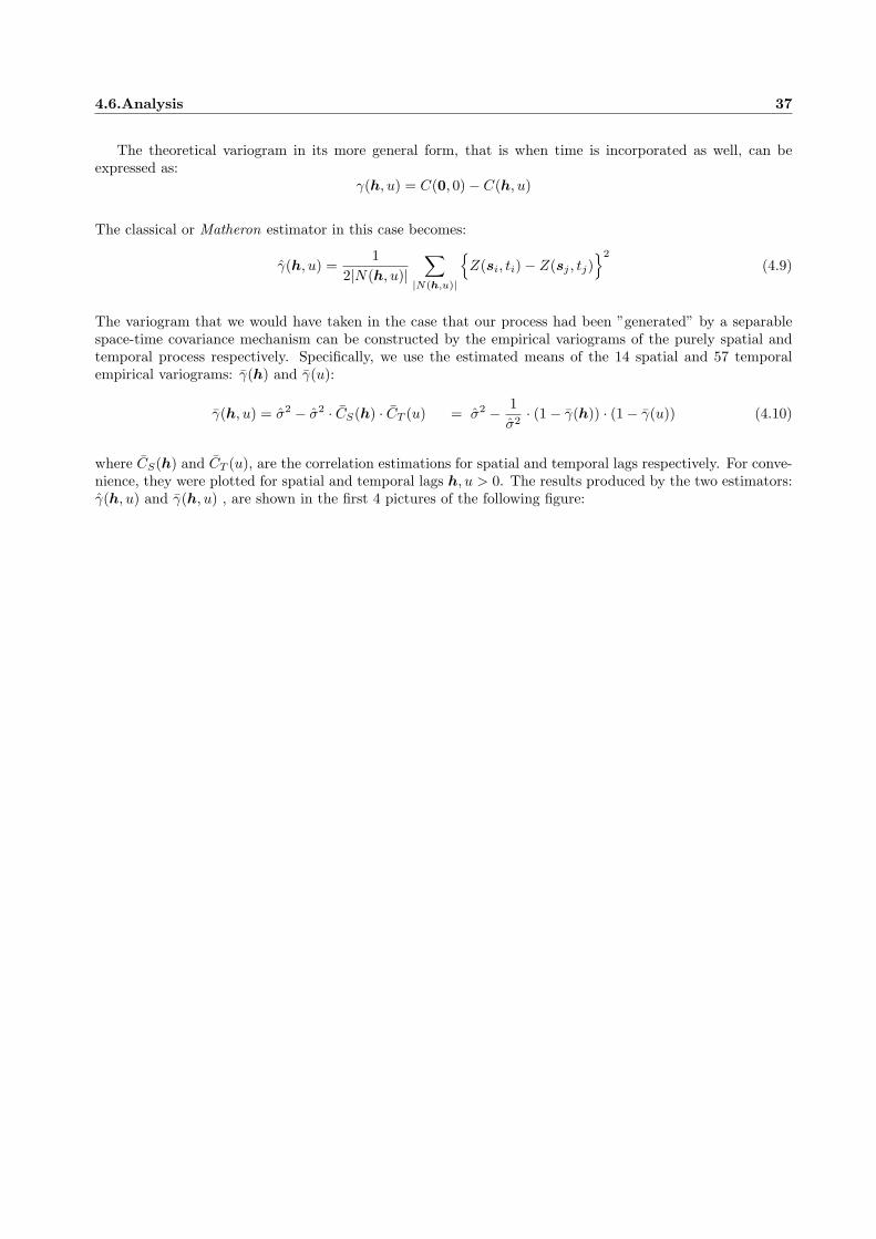
4.6.Analysis 37

The theoretical variogram in its more general form, that is when time is incorporated as well, can beexpressed as:

γ(h, u) = C(0, 0)− C(h, u)

The classical or Matheron estimator in this case becomes:

γ(h, u) =1

2|N(h, u)|∑

|N(h,u)|

{Z(si, ti)− Z(sj , tj)

}2

(4.9)

The variogram that we would have taken in the case that our process had been ”generated” by a separablespace-time covariance mechanism can be constructed by the empirical variograms of the purely spatial andtemporal process respectively. Specifically, we use the estimated means of the 14 spatial and 57 temporalempirical variograms: γ(h) and γ(u):

γ(h, u) = σ2 − σ2 · CS(h) · CT (u) = σ2 − 1σ2

· (1− γ(h)) · (1− γ(u)) (4.10)

where CS(h) and CT (u), are the correlation estimations for spatial and temporal lags respectively. For conve-nience, they were plotted for spatial and temporal lags h, u > 0. The results produced by the two estimators:γ(h, u) and γ(h, u) , are shown in the first 4 pictures of the following figure:

4.6.Analysis 38

0.0 0.2 0.4 0.6 0.8 1.0

0.0

0.2

0.4

0.6

0.8

1.0

Space lag

Tim

e la

g

Space lag

Tim

e la

g

0.0 0.2 0.4 0.6 0.8 1.0

0.0

0.2

0.4

0.6

0.8

1.0

0.0 0.2 0.4 0.6 0.8 1.0

0.0

0.2

0.4

0.6

0.8

1.0

Space lag

Tim

e la

g

Space lag

Tim

e la

g

0.0 0.2 0.4 0.6 0.8 1.0

0.0

0.2

0.4

0.6

0.8

1.0

0.0 0.2 0.4 0.6 0.8 1.0

0.0

0.2

0.4

0.6

0.8

1.0

Space lag

Tim

e la

g

Space lag

Tim

e la

g

0.0 0.2 0.4 0.6 0.8 1.0

0.0

0.2

0.4

0.6

0.8

1.0

Figure 4.6, a and b: Image and contour plots of the space-time empirical variograms a) Of the observedprocess, γ(h, u) and b) Of the observed process that would be produced in the case that it was separable, γ(h, u).c) Theoretical variogram of the fitted separable model, γSep(h, u)

We can see an obvious similarity in the distribution of colours between the first two image plots, while thepatterns produced in the first two contour ones do not seem to be substantially different. In other words, thereis an empirical evidence for the fact that a separable model is likely to give an as good fit as the particularnon-separable one that we chose. For this reason, in the third part of the same image we plotted the respectiveimage and contour plots of the theoretical space-time variogram of the separable model (4.5).

γSep(h, u) = σ2 − CNS(h, u) d=0 (4.11)

where CNS(h, u) d=0 = CS(h) · CT (u) is the separable covariance function (4.5).The theoretical model γSep(h, u) appears to give a good fit to the observed empirical spatio-temporal

variogram γ(h, u) (figure 4.6a).Although the results appeared to be quite unexpected, they were only based on empirical justifications.

We now investigate the separability hypothesis H2 : d = 0 and the alternative one H3 : d > 0, by trying tomake an estimation of the d parameter from the data and inspecting whether its value is significantly differentfrom zero.

A ”direct” inference of d proved to be a quite difficult task mainly due to the high complexity of the modeland the large number of data. For this reason we calculated its log-likelihood for different values of d and tried

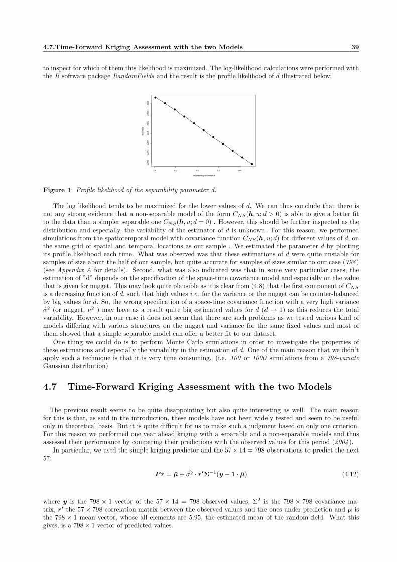
4.7.Time-Forward Kriging Assessment with the two Models 39

to inspect for which of them this likelihood is maximized. The log-likelihood calculations were performed withthe R software package RandomFields and the result is the profile likelihood of d illustrated below:

●

●

●

●

●

●

●

●

●

●

●

0.0 0.2 0.4 0.6 0.8

−22

90−

2285

−22

80−

2275

−22

70−

2265

−22

60

seperablity parameter d

likel

ihoo

d

Figure 1: Profile likelihood of the separability parameter d.

The log likelihood tends to be maximized for the lower values of d. We can thus conclude that there isnot any strong evidence that a non-separable model of the form CNS(h, u; d > 0) is able to give a better fitto the data than a simpler separable one CNS(h, u; d = 0) . However, this should be further inspected as thedistribution and especially, the variability of the estimator of d is unknown. For this reason, we performedsimulations from the spatiotemporal model with covariance function CNS(h, u; d) for different values of d, onthe same grid of spatial and temporal locations as our sample . We estimated the parameter d by plottingits profile likelihood each time. What was observed was that these estimations of d were quite unstable forsamples of size about the half of our sample, but quite accurate for samples of sizes similar to our case (798 )(see Appendix A for details). Second, what was also indicated was that in some very particular cases, theestimation of ”d” depends on the specification of the space-time covariance model and especially on the valuethat is given for nugget. This may look quite plausible as it is clear from (4.8) that the first component of CNS

is a decreasing function of d, such that high values i.e. for the variance or the nugget can be counter-balancedby big values for d. So, the wrong specification of a space-time covariance function with a very high varianceσ2 (or nugget, ν2 ) may have as a result quite big estimated values for d (d → 1) as this reduces the totalvariability. However, in our case it does not seem that there are such problems as we tested various kind ofmodels differing with various structures on the nugget and variance for the same fixed values and most ofthem showed that a simple separable model can offer a better fit to our dataset.

One thing we could do is to perform Monte Carlo simulations in order to investigate the properties ofthese estimations and especially the variability in the estimation of d. One of the main reason that we didn’tapply such a technique is that it is very time consuming. (i.e. 100 or 1000 simulations from a 798-variateGaussian distribution)

4.7 Time-Forward Kriging Assessment with the two Models

The previous result seems to be quite disappointing but also quite interesting as well. The main reasonfor this is that, as said in the introduction, these models have not been widely tested and seem to be usefulonly in theoretical basis. But it is quite difficult for us to make such a judgment based on only one criterion.For this reason we performed one year ahead kriging with a separable and a non-separable models and thusassessed their performance by comparing their predictions with the observed values for this period (2004 ).

In particular, we used the simple kriging predictor and the 57× 14 = 798 observations to predict the next57:

Pr = µ+ σ2 · r′Σ−1(y − 1 · µ) (4.12)

where y is the 798 × 1 vector of the 57 × 14 = 798 observed values, Σ2 is the 798 × 798 covariance ma-trix, r′ the 57× 798 correlation matrix between the observed values and the ones under prediction and µ isthe 798 × 1 mean vector, whose all elements are 5.95, the estimated mean of the random field. What thisgives, is a 798× 1 vector of predicted values.

4.7.Time-Forward Kriging Assessment with the two Models 40

The procedure was repeated four times. The first time this was performed by considering a separable space-time covariance function: Σ2

ij = CNS d=0 and it was repeated for three different values for the separability(interaction) parameter d: 0.25, 0.5 and 0.95.

The mean absolute and squared prediction errors are given in the following table:

M.A.E. M.S.E M.O.P. M.O.V. V.O.P.Separable Model d=0 4.698 37.229 10.432 9.9 7.388

Non-Separable Model d=0.25 4.825 38.746 10.217 9.9 5.922Non-Separable Model d=0.5 4.946 40.271 9.994 9.9 4.770Non-Separable Model d=0.95 5.154 42.914 9.612 9.9 3.251

Table 4.7 Mean of squared (MSE) and absolute (MAE) prediction errors ,the mean of the predictions (M.O.P),the mean of the observed values at this period (M.O.V.) and the variance of the predictions (V.O.P.), for eachof the four models

It is clear once more that the model with no space-time interactions provides better fit than the othermodels. The mean absolute (MAE) and squared prediction errors (MSE) tend to increase as d increases, thatis when the space- time interactions parameter becomes greater. The table also includes the mean (MOP)and the variance (VOP) of the predicted vector as well as the mean of the real observations at this period(MOV). We observe that the mean of the predictions is quite close to the mean of the data at this year whilethe variability in the prediction increases as the space and time interactions decreases. The four box plotsbelow show that there are not any significant outliers in the absolute errors:

●

●

●

●

●

●

●

●●

●

●

●

●

●

●

●

●

●●

05

1015

Seperable & Non_Seperable models

Figure 4.72: Boxplots of the absolute prediction errors, with the separable and the non-separable modelsrespectively: d=0,0.25,0.5,0.95

The differences in the predictions between the four models can be illustrated in the following figure, thatshows the observed values of the year 2004 and the predictions performed with all of the four models.

●

●

●

● ●

●

● ●

● ●

●

●

●

●

●

●

●

●

●

●

●

●

●

●

●

●

●

● ●

●

●

●

●

●

●

●

●

●

●

●

●

●

●

● ●

●

●

● ●

●

●

●

●

●

●

● ●

0 10 20 30 40 50

−5

05

1015

2025

Locations

Pre

dict

ions

●

●●

●

●

●

●●

●

●

●

●

●

●

● ●

●

●●

●

●

●

●

●

●

●

●

●

●

● ●●

●

●

●

●

●

●

●

●●

●

●●

●

●

●

●

●

●

●

●

●

●

●

●●

●

●●

●

●

●

●●

●●

●

●

●

●

● ●

●

● ●

●

●

●

●

●

●

●

●

●

●

●●

●

●

●

●

●

●

●

●

●●

●

●●

●

●

●

●

●

●

●

●

●

●

●

● ●

●

● ●

●●

●

●●

●●

●

●

●

●

●●

●

● ●

●

●

●

●●

●

●

●

●

●

●●

●

●

●

●

●

●

●

●

●●

●

●●

●

●

●

●

●

●

●●

●

●

●

● ●

●

● ●

● ●

●

● ●

● ●

●●

●

●

●●

●

●●

●

●

●

● ●

●

●

●

●

●

●

●●

●

●

●

●

●

●

●

●●

●

●●

●

●

●

●

●

●

● ● ●

●

●

● ●

REALd=0d=0.25d=0.5d=0.95

4.7.Time-Forward Kriging Assessment with the two Models 41

Figure 4.73: Predictions with a non-separable model with various degrees of space-time interactions: d=0,0.25,0.5,0.95and the real values (red)

Figure ... is a map showing the spatial variability in the prediction differences between the models withd = 0 and d = 0.5

−9 −8 −7 −6 −5

3738

3940

41

Coord X

Coo

rd Y

●

●●●●●

●●●●

●● ●●●●

●●

●●

●●

●●●●

●●

●●●●●●●●●●●●●

●●●●●● ●

●●●●●●● ●●

2.11.16.8e−06

Figure 4.74a: Difference in the predictive values for the models with space-time interaction parameter d=0and d=0.5

Finally we provide some figures showing the three years ahead predictions with a separable d = 0 and anon-separable model d = 0.5 in the whole area outside the Portuguese coast. The results are shown below, aswell as the differences in these predictions in a separate figure.

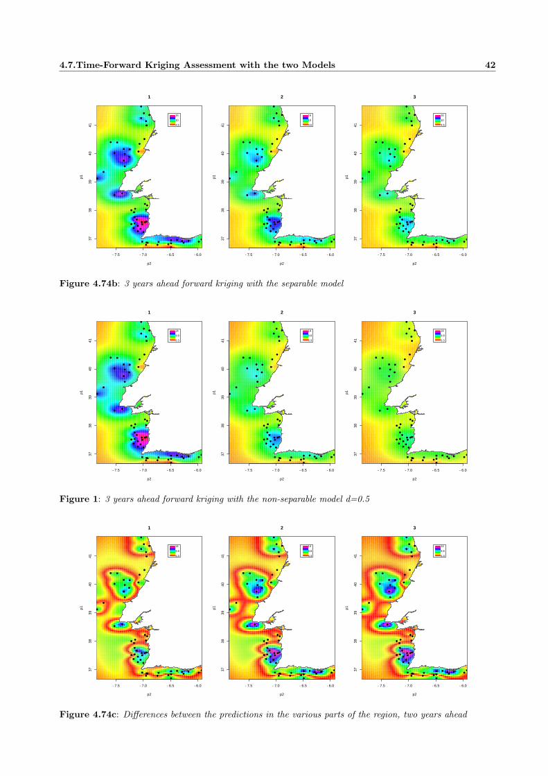
4.7.Time-Forward Kriging Assessment with the two Models 42

−7.5 −7.0 −6.5 −6.0

3738

3940

41

1

p2

p1

●

●●

●

●

●

●

●●●

●●

●

●●

●

●

●

●

●

●●

●●

●●

●

●

●

●

●● ●●

●●

●

●●

●●

●●●

●

●

●

●

●●

● ●●

●

●●

●

16

10

4.6

−7.5 −7.0 −6.5 −6.0

3738

3940

41

2

p2

p1

●

●●

●

●

●

●

●●●

●●

●

●●

●

●

●

●

●

●●

●●

●●

●

●

●

●

●● ●●

●●

●

●●

●●

●●●

●

●

●

●

●●

● ●●

●

●●

●

16

10

4.6

−7.5 −7.0 −6.5 −6.0

3738

3940

41

3

p2

p1

●

●●

●

●

●

●

●●●

●●

●

●●

●

●

●

●

●

●●

●●

●●

●

●

●

●

●● ●●

●●

●

●●

●●

●●●

●

●

●

●

●●

● ●●

●

●●

●

16

10

4.6

Figure 4.74b: 3 years ahead forward kriging with the separable model

−7.5 −7.0 −6.5 −6.0

3738

3940

41

1

p2

p1

●

●●

●

●

●

●

●●●

●●

●

●●

●

●

●

●

●

●●

●●

●●

●

●

●

●

●● ●●

●●

●

●●

●●

●●●

●

●

●

●

●●

● ●●

●

●●

●

14

9.8

5.3

−7.5 −7.0 −6.5 −6.0

3738

3940

41

2

p2

p1

●

●●

●

●

●

●

●●●

●●

●

●●

●

●

●

●

●

●●

●●

●●

●

●

●

●

●● ●●

●●

●

●●

●●

●●●

●

●

●

●

●●

● ●●

●

●●

●

14

9.8

5.3

−7.5 −7.0 −6.5 −6.0

3738

3940

41

3

p2

p1

●

●●

●

●

●

●

●●●

●●

●

●●

●

●

●

●

●

●●

●●

●●

●

●

●

●

●● ●●

●●

●

●●

●●

●●●

●

●

●

●

●●

● ●●

●

●●

●

14

9.8

5.3

Figure 1: 3 years ahead forward kriging with the non-separable model d=0.5

−7.5 −7.0 −6.5 −6.0

3738

3940

41

1

p2

p1

●

●●

●

●

●

●

●●●

●●

●

●●

●

●

●

●

●

●●

●●

●●

●

●

●

●

●● ●●

●●

●

●●

●●

●●●

●

●

●

●

●●

● ●●

●

●●

●

14

9.8

5.3

−7.5 −7.0 −6.5 −6.0

3738

3940

41

2

p2

p1

●

●●

●

●

●

●

●●●

●●

●

●●

●

●

●

●

●

●●

●●

●●

●

●

●

●

●● ●●

●●

●

●●

●●

●●●

●

●

●

●

●●

● ●●

●

●●

●

14

9.8

5.3

−7.5 −7.0 −6.5 −6.0

3738

3940

41

3

p2

p1

●

●●

●

●

●

●

●●●

●●

●

●●

●

●

●

●

●

●●

●●

●●

●

●

●

●

●● ●●

●●

●

●●

●●

●●●

●

●

●

●

●●

● ●●

●

●●

●

14

9.8

5.3

Figure 4.74c: Differences between the predictions in the various parts of the region, two years ahead

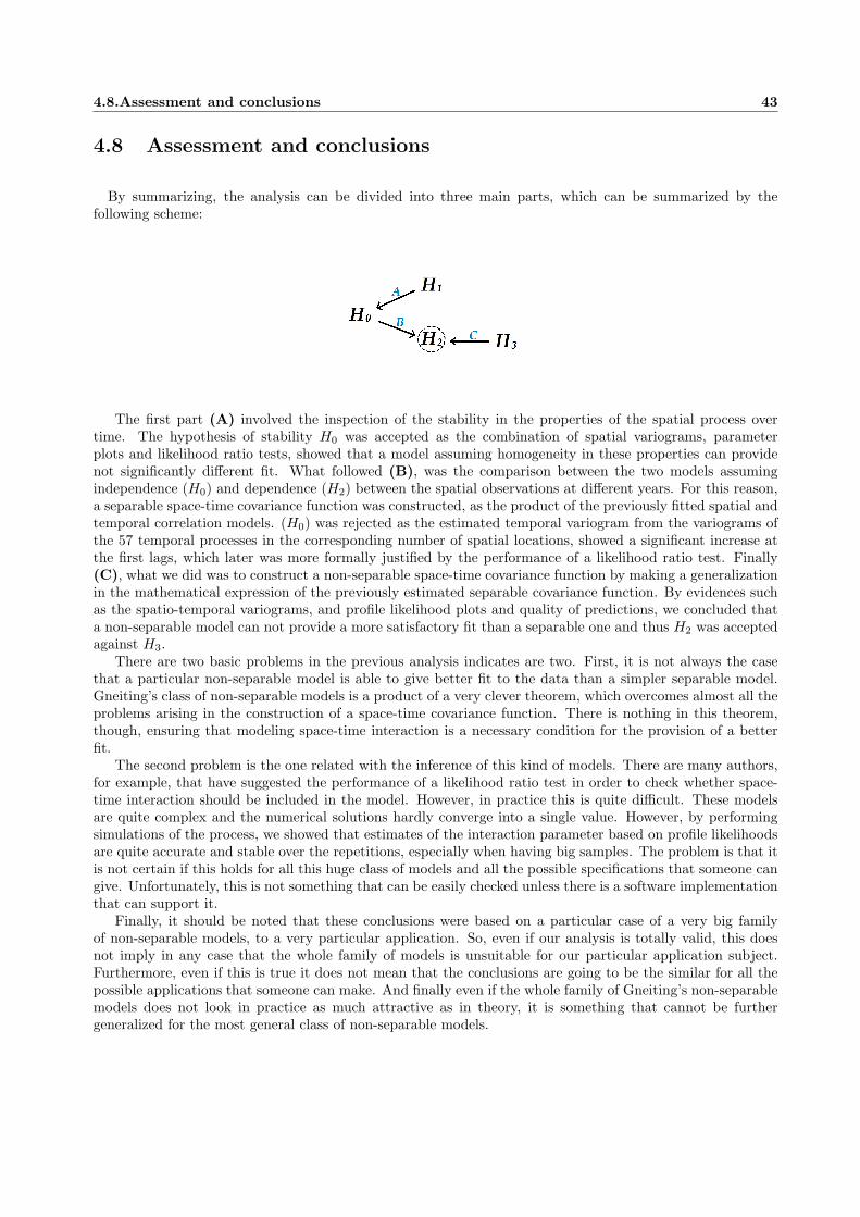
4.8.Assessment and conclusions 43

4.8 Assessment and conclusions

By summarizing, the analysis can be divided into three main parts, which can be summarized by thefollowing scheme:

The first part (A) involved the inspection of the stability in the properties of the spatial process overtime. The hypothesis of stability H0 was accepted as the combination of spatial variograms, parameterplots and likelihood ratio tests, showed that a model assuming homogeneity in these properties can providenot significantly different fit. What followed (B), was the comparison between the two models assumingindependence (H0) and dependence (H2) between the spatial observations at different years. For this reason,a separable space-time covariance function was constructed, as the product of the previously fitted spatial andtemporal correlation models. (H0) was rejected as the estimated temporal variogram from the variograms ofthe 57 temporal processes in the corresponding number of spatial locations, showed a significant increase atthe first lags, which later was more formally justified by the performance of a likelihood ratio test. Finally(C), what we did was to construct a non-separable space-time covariance function by making a generalizationin the mathematical expression of the previously estimated separable covariance function. By evidences suchas the spatio-temporal variograms, and profile likelihood plots and quality of predictions, we concluded thata non-separable model can not provide a more satisfactory fit than a separable one and thus H2 was acceptedagainst H3.

There are two basic problems in the previous analysis indicates are two. First, it is not always the casethat a particular non-separable model is able to give better fit to the data than a simpler separable model.Gneiting’s class of non-separable models is a product of a very clever theorem, which overcomes almost all theproblems arising in the construction of a space-time covariance function. There is nothing in this theorem,though, ensuring that modeling space-time interaction is a necessary condition for the provision of a betterfit.

The second problem is the one related with the inference of this kind of models. There are many authors,for example, that have suggested the performance of a likelihood ratio test in order to check whether space-time interaction should be included in the model. However, in practice this is quite difficult. These modelsare quite complex and the numerical solutions hardly converge into a single value. However, by performingsimulations of the process, we showed that estimates of the interaction parameter based on profile likelihoodsare quite accurate and stable over the repetitions, especially when having big samples. The problem is that itis not certain if this holds for all this huge class of models and all the possible specifications that someone cangive. Unfortunately, this is not something that can be easily checked unless there is a software implementationthat can support it.

Finally, it should be noted that these conclusions were based on a particular case of a very big familyof non-separable models, to a very particular application. So, even if our analysis is totally valid, this doesnot imply in any case that the whole family of models is unsuitable for our particular application subject.Furthermore, even if this is true it does not mean that the conclusions are going to be the similar for all thepossible applications that someone can make. And finally even if the whole family of Gneiting’s non-separablemodels does not look in practice as much attractive as in theory, it is something that cannot be furthergeneralized for the most general class of non-separable models.

Chapter 5

Concluding Remarks and FurtherStudies

Environmental and geophysical processes such as atmospheric pollutant concentrations, precipitation fieldsand surface winds are characterized by spatial and temporal variability. Such kind of space-time fields aregenerally thought to be ”random”, paradoxically a view that is not consistent with physical laws. These lawsare not fully understood and their complexity does not usually allow for a precise deterministic description ofa given situation. Stochastic models on the other hand are based typically on a small number of parametersthat can be inferred or modeled. They aim at building a process that mimics some patterns of the observedspatio-temporal variability,without necessarily following the governing equations.

Spatio(-Temporal) phenomena are characterized by their uniqueness and their non-reproducibility. Whatwe observe most times is a single replication from a particular assumed stochastic mechanism. Consequently,inference most times is proved to be a quite complicated task and very often impossible without the adoptionof simplifications and assumptions.

The principles in the analysis of spatio-temporal processes are not that different from the ones in the purelyspatial case. However, the physical difference between space and time sets a further number of difficulties andassumptions.

The need for recognizing that space and time are two completely different notions has as a cost our difficultyin specifying valid spatio-temporal covariance functions. A very common approach is based on the valididnessof the products of ”separate” covariance functions to represent valid covariance functions as well. Despite theadvantages of this method, its greatest disadvantage is that it does not allow for the incorporation of space-time interactions. Unfortunately there is a great scarcity of non-separable covariance models. Most of theapproaches in the construction of such kind of models are based on Fourier integral analysis and operations inthe spectral domain. We investigated one of the most popular approaches, Gneiting ’s class of stationary andfully symmetric covariance functions. Gneiting proposed a methodology according to which the specificationof space-time covariance functions does not rely on Fourier integral analysis. Instead, it is based on explicitparametric covariance models and at the same time, space and time are allowed to interact.

Our main concern in the last chapter of the project was to check whether this family of models is practicallyuseful for the modeling of fish stock data, over the period of 14 years in the Portuguese coast. We followeda particular methodology in order to show that a joint space-time analysis is capable to be applied to oursample and moreover, we showed that it provides a better fit than analyzing the data separately for eachtime period. Finally we tried to make an assessment of how much better is the fit provided by Gneiting ’snon-separable space-time covariance function. This was made possible by the support of the recent and stillunder development R software package RandomFields, which makes possible the construction of a particularcovariance function of Gneiting ’s class, which is the one that we used in the analysis. The assessment wasbased on spatio-temporal variograms, profile likelihoods plots for the space-time interaction parameters andcomparison of the one year ahead kriging predictions with the actual observations of at the last year. However,all the evidences supported the acceptance of the separability hypothesis. Models with lower rates of spaceand time interactions appear to give better fit and better predictions as well.

Unfortunately, despite all these results, none of the problems regarding the appropriateness for this par-ticular class of models have been solved and the fact that we ended up in H2 (separability) did not satisfyour initial questions. What we tested and concluded was the relative appropriateness between two particularspace-time covariance models and not between two different classes of models.

44

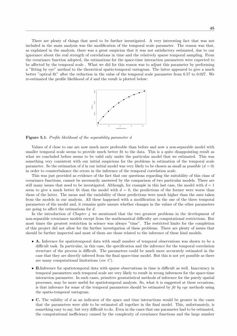
45

There are plenty of things that need to be further investigated. A very interesting fact that was notincluded in the main analysis was the modification of the temporal scale parameter. The reason was that,as explained in the analysis, there was a great suspicion that it was not satisfactory estimated, due to ourignorance about the real strength of correlations in time and the relatively sparse temporal sampling. Fromthe covariance function adopted, the estimations for the space-time interaction parameters were expected tobe affected by the temporal scale . What we did for this reason was to adjust this parameter by performinga ”fitting by eye” method to the theoretical spatio-temporal variogram. The latter appeared to give a muchbetter ”optical fit” after the reduction in the value of the temporal scale parameter from 0.57 to 0.027. Were-estimated the profile likelihood of d and the result is plotted below:

●

●

●

●

●

●

●

●

●

●

0.0 0.2 0.4 0.6 0.8

−22

40.5

−22

40.0

−22

39.5

seperablity parameter d

likel

ihoo

d

Figure 5.1: Profile likelihood of the separability parameter d

Values of d close to one are now much more preferable than before and now a non-separable model withsmaller temporal scale seems to provide much better fit to the data. This is a quite disappointing result aswhat we concluded before seems to be valid only under the particular model that we estimated. This wassomething very consistent with our initial suspicions for the problems in estimation of the temporal scaleparameter. So the estimation of d in our initial model was very likely to be chosen as small as possible (d = 0)in order to counterbalance the errors in the inference of the temporal correlation scale.

This was just provided as evidence of the fact that our questions regarding the suitability of this class ofcovariance functions, cannot be necessarily answered by the comparison of two particular models. There arestill many issues that need to be investigated. Although, for example in this last case, the model with d = 1seem to give a much better fit than the model with d = 0, the predictions of the former were worse thanthose of the latter. The mean and the variability of these predictions were much higher than the ones takenfrom the models in our analysis. All these happened with a modification in the one of the three temporalparameters of the model and, it remains quite unsure whether changes in the values of the other parametersare going to affect the estimations for d.

In the introduction of Chapter 4 we mentioned that the two greatest problems in the development ofnon-separable covariance models except from the mathematical difficulty are computational restrictions. Butmost times the greatest restriction in science was always ”time”. The restricted limits for the completionof this project did not allow for the further investigation of these problems. There are plenty of issues thatshould be further inspected and most of them are those related to the inference of these kind models.

• A. Inference for spatiotemporal data with small number of temporal observations was shown to be adifficult task. In particular, in this case, the specification and the inference for the temporal correlationstructure of the process is difficult. The parameters could be much more accurately estimated in thecase that they are directly inferred from the final space-time model. But this is not yet possible as thereare many computational limitations (see C ).

• B.Inference for spatiotemporal data with sparse observations in time is difficult as well. Inaccuracy intemporal parameters such temporal scale are very likely to result in wrong inferences for the space-timeinteraction parameter. In such cases, primitive geostatistical methods of inference for the purely spatialprocesses, may be more useful for spatiotemporal analysis. So, what it is suggested at these occasions,is that inference for some of the temporal parameters should be estimated by fit by eye methods usingthe spatio-temporal variogram.

• C. The validity of d as an indicator of the space and time interactions would be greater in the casesthat the parameters were able to be estimated all together in the final model. This, unfortunately, issomething easy to say, but very difficult to do. Even in the cases that one parameter had to be estimated,the computational inefficiency caused by the complexity of covariance functions and the large number

46

of observations, was great. The convergence in the numerical algorithms were hardly achieved and thefinal estimated values, were quite often very close to their boundary limits.

They do not converge and even for the case of one parameter we saw that we needed to plot the profilelikelihood. Sufficient inference is something of vital importance as the estimated values of d seem to berelated with the values of the other parameters.

• D. The variability in the estimations of space-time interaction parameter should be investigated, as wellas all the factors that affect it. It should be in general inspected under which circumstances such kindof parameters can be estimated well. By simulations performed with these models, it was proved thatsmall changes in the number of sample size had significant results in the variability of estimations.

On the other hand, Monte Carlo methods require much time due to the large number of data andvery often simulations from models with complex covariance structures are impossible. However, thedevelopment in this area at this moment is in a more advanced stage.

• E. Once more we should emphasize the need of applying these models into different application areas.Different models usually perform better in different applications. In our case, for example, there is nophysical indication that the decay in the spatial correlation between the fish stock should be a functionof the temporal lag, which was one of the assumptions of the model that we applied. So, one conclusionthan can be drawn here is the fact that space takes into account time through the spatial scale doesnot necessarily mean that the incorporation of space-time interactions is going to solve all the problems.This is only a particular case of space time interactions.

On the other hand, such a model could be quite realistic in the case of monitoring fish stocks of acontaminated area. It would be quite plausible for someone to assume that the released chemicalsmay have caused physical differences in the behaviour of fish over time. This may have as a result,their number at a particular location to be for example much less affected by those in the neighbouringlocations for different time lags. So, a model assuming a spatial scale to be a function of the temporal lagis likely to give a much better fit than a separable model. So, the conclusions regarding the suitabilityof the same model could be much different at this case.

Generalizations regarding the suitability of this family of non-separable models being based on only oneapplication, seems to be as hard as our efforts to study the properties of a particular process relyingonly on its single realization.

Estimations for the space-time interaction parameter d proved to be very sensitive to the model specifi-cations and very much related to the estimated values of the other parameters of the model. Our personalopinion here is that the estimated values for d do not reveal anything about whether the theoretical mechanismthat ”generated” a process is separable or not. Most times the estimated values of this parameter seem tobe ”chosen” such that either the mistakes in inference of the previously estimated parameters are ”corrected”or errors in model mispecifications are ”recovered”. Probably this may change in the case that all the modelparameters are able to be inferred together.

Gneiting’s class of models is really a very clever theoretical device, but it is uncertain whether it proves tobe useful in practice. In Chapter 3, the need for overcoming the mathematical restrictions in the productionof valid covariance functions was so much emphasized. Here, it should be also emphasized that even if a”mathematical expert” is able to solve this problem in one day, the great difficulties currently existing inthe spatio-temporal geostatistical modeling will never be solved unless all these ”new” models that will beproduced, are not practically tested in a real-life problems, such as here.

After all these discussions, the greatest contribution of this project was not turned out to be its assess-ment for the suitability of different space-time covariance models, but rather its contribution to our furtherfamiliarity with the statement that what is really sure that we know is the fact that we don’t know. The mostgeneral conclusion that we can make at this last part of the project, is that the path to the full developmentof spatio-temporal geostatistical models seems to be quite long and the obstacles appear to be many. Untilthis stage, the real world is going to remain much more complex than our assumptions and the settlement ofreal life problems will necessarily require the adoption of simple space-time describing mechanisms. Althoughspace-time processes are yet difficult to be satisfactory described by means of the existing mathematicalmechanisms, our attempts in the solution of real life problems will seem to be fully characterised by AbrahamMaslow ’s words and his recognition of the fact that ”when the only tool that you have is a hammer, thenevery problem begins to look like nail”.

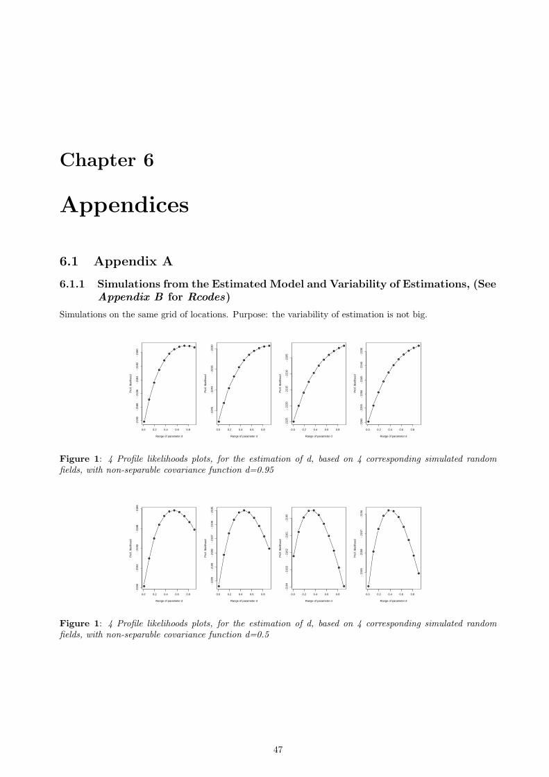
Chapter 6

Appendices

6.1 Appendix A

6.1.1 Simulations from the Estimated Model and Variability of Estimations, (SeeAppendix B for Rcodes)

Simulations on the same grid of locations. Purpose: the variability of estimation is not big.

●

●

●

●

●

●

●

●● ●

●

0.0 0.2 0.4 0.6 0.8

−21

90−

2188

−21

86−

2184

−21

82−

2180

Range of parameter d

Pro

f. lik

elih

ood

●

●

●

●

●

●

●

●

●● ●

0.0 0.2 0.4 0.6 0.8

−22

45−

2240

−22

35−

2230

Range of parameter d

Pro

f. lik

elih

ood

●

●

●

●

●

●

●

●

●

●

●

0.0 0.2 0.4 0.6 0.8

−22

25−

2220

−22

15−

2210

−22

05

Range of parameter d

Pro

f. lik

elih

ood

●

●

●

●

●

●

●

●

●

●

●

0.0 0.2 0.4 0.6 0.8

−22

60−

2255

−22

50−

2245

−22

40−

2235

Range of parameter d

Pro

f. lik

elih

ood

Figure 1: 4 Profile likelihoods plots, for the estimation of d, based on 4 corresponding simulated randomfields, with non-separable covariance function d=0.95

●

●

●

●

●

●●

●

●

●

●

0.0 0.2 0.4 0.6 0.8

−21

94−

2192

−21

90−

2188

−21

86

Range of parameter d

Pro

f. lik

elih

ood

●

●

●

●

●

●●

●

●

●

●

0.0 0.2 0.4 0.6 0.8

−22

00−

2199

−21

98−

2197

−21

96−

2195

Range of parameter d

Pro

f. lik

elih

ood

●

●

●

● ●

●

●

●

●

●

●

0.0 0.2 0.4 0.6 0.8

−21

64−

2163

−21

62−

2161

−21

60

Range of parameter d

Pro

f. lik

elih

ood

●

●

●

●

● ●

●

●

●

●

●

0.0 0.2 0.4 0.6 0.8

−21

59−

2158

−21

57−

2156

Range of parameter d

Pro

f. lik

elih

ood

Figure 1: 4 Profile likelihoods plots, for the estimation of d, based on 4 corresponding simulated randomfields, with non-separable covariance function d=0.5

47

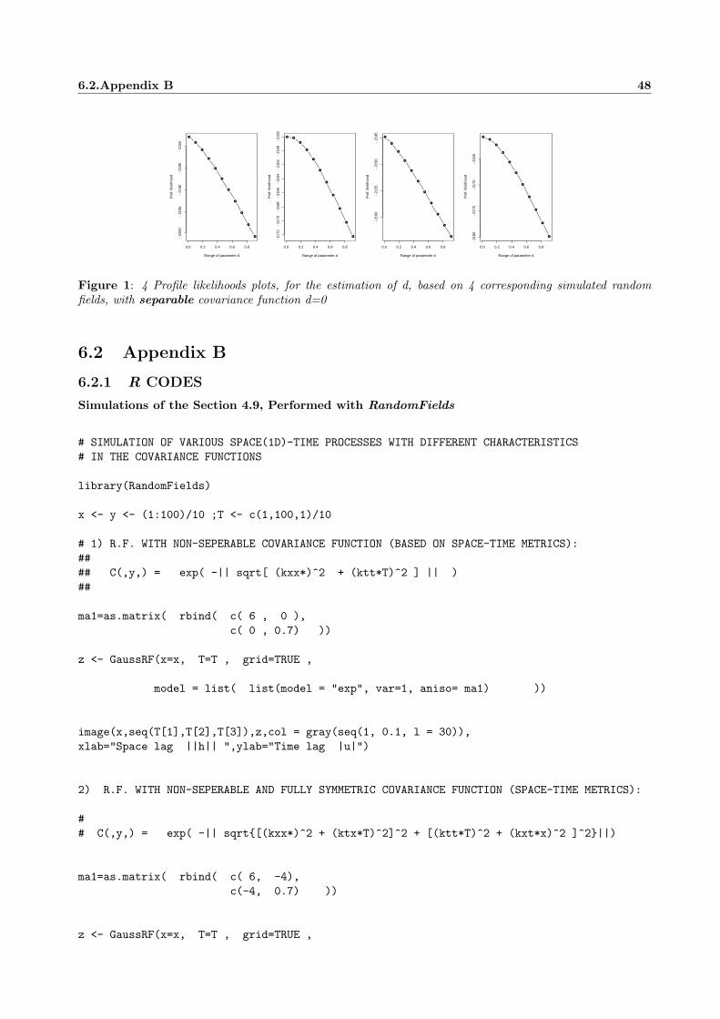
6.2.Appendix B 48

●

●

●

●

●

●

●

●

●

●

●

0.0 0.2 0.4 0.6 0.8

−22

00−

2195

−21

90−

2185

−21

80

Range of parameter d

Pro

f. lik

elih

ood

● ●

●

●

●

●

●

●

●

●

●

0.0 0.2 0.4 0.6 0.8

−21

72−

2170

−21

68−

2166

−21

64−

2162

−21

60−

2158

Range of parameter d

Pro

f. lik

elih

ood

●

●

●

●

●

●

●

●

●

●

●

0.0 0.2 0.4 0.6 0.8

−21

60−

2155

−21

50−

2145

Range of parameter d

Pro

f. lik

elih

ood

●●

●

●

●

●

●

●

●

●

●

0.0 0.2 0.4 0.6 0.8

−21

80−

2175

−21

70−

2165

Range of parameter d

Pro

f. lik

elih

ood

Figure 1: 4 Profile likelihoods plots, for the estimation of d, based on 4 corresponding simulated randomfields, with separable covariance function d=0

6.2 Appendix B

6.2.1 R CODES

Simulations of the Section 4.9, Performed with RandomFields

# SIMULATION OF VARIOUS SPACE(1D)-TIME PROCESSES WITH DIFFERENT CHARACTERISTICS# IN THE COVARIANCE FUNCTIONS

library(RandomFields)

x <- y <- (1:100)/10 ;T <- c(1,100,1)/10

# 1) R.F. WITH NON-SEPERABLE COVARIANCE FUNCTION (BASED ON SPACE-TIME METRICS):#### C(,y,) = exp( -|| sqrt[ (kxx*)^2 + (ktt*T)^2 ] || )##

ma1=as.matrix( rbind( c( 6 , 0 ),c( 0 , 0.7) ))

z <- GaussRF(x=x, T=T , grid=TRUE ,

model = list( list(model = "exp", var=1, aniso= ma1) ))

image(x,seq(T[1],T[2],T[3]),z,col = gray(seq(1, 0.1, l = 30)),xlab="Space lag ||h|| ",ylab="Time lag |u|")

2) R.F. WITH NON-SEPERABLE AND FULLY SYMMETRIC COVARIANCE FUNCTION (SPACE-TIME METRICS):

## C(,y,) = exp( -|| sqrt{[(kxx*)^2 + (ktx*T)^2]^2 + [(ktt*T)^2 + (kxt*x)^2 ]^2}||)

ma1=as.matrix( rbind( c( 6, -4),c(-4, 0.7) ))

z <- GaussRF(x=x, T=T , grid=TRUE ,

6.2.Appendix B 49

model = list( list(model = "exp", var=1, aniso= ma1) ))

image(x,seq(T[1],T[2],T[3]),z,col = gray(seq(1, 0.1, l = 30)),xlab="Space lag ||h|| ",ylab="Time lag |u|")

3) R.F. WITH SEPERABLE COVARIANCE FUNCTION (PRODUCT OF COV.F):### C(,y,) = exp( -|| kx*|| || ) * exp( -|| kt*|T| || )

par(mfrow=c(1,2))

ma1=as.matrix( rbind( c(4, 0),c(0, 0)

))ma2=as.matrix( rbind( c(0, 0),

c(0, 2) ))

z <- GaussRF(x=x, T=T , grid=TRUE ,

model = list( list(model = "exp", var=1, aniso= ma1),"*",list(model = "exp", var=1, aniso= ma2) ))

image(x,seq(T[1],T[2],T[3]),z,col = gray(seq(1, 0.1, l = 30)),xlab="Space lag ||h|| ",ylab="Time lag |u|")

4) R.F. WITH SEPERABLE COVARIANCE FUNCTION (SUM OF COV.F.):

# C(,y,) = exp( -|| k1*|| || ) + exp( -|| k2*|T| || )

ma1=as.matrix( rbind( c(4, 0),c(0, 0)

))ma2=as.matrix( rbind( c(0, 0),

c(0, 2) ))

z <- GaussRF(x=x, T=T , grid=TRUE ,

model = list( list(model = "exp", var=1, aniso= ma1),"+",list(model = "exp", var=1, aniso= ma2) ))

image(x,seq(T[1],T[2],T[3]),z,col = gray(seq(1, 0.1, l = 30)),xlab="Space lag ||h|| ",ylab="Time lag |u|")

#^ ^ ^ ^ ^ ^ ^ ^ ^ ^ ^ ^ ^ ^ ^ ^ ^ ^ ^ ^ ^ ^ ^ ^ ^ ^ ^ ^ ^ ^ ^ ^ ^ ^ ^ ^ ^ ^ ^ ^ ^ ^ ^ ^ ^ ^ ^ ^

6.3.Simulating from the Estimated Model and Computation of the P.Likelihood of theSeperability Parameter 50

6.3 Simulating from the Estimated Model and Computation of theP.Likelihood of the Seperability Parameter

# SIMULATING FROM THE NON-SEPERABLE, IN COVARIANCE FUNCTION, ESTIMATED MODEL INTO THE SAME# GRID OF THE DATA LOCATIONS AND CALCULATING THE PROFILE LIKELIHOOD OF THE SEPERABILITY PARAMETER

require(RandomFields)

attach(hake.cc) # DATASET

Hx=hake.cc[,7][1:57]Hy=hake.cc[,3][1:57]

# initial, maximum, & increments --> for "d"yr2004=2003 ; d=0.01 ; mx=1 ; dst=0.09

MEAN=5.95alphaStable = 1.141 ; alphaGC = 1.52

betaGC = 1.44scaleStable = 4.04 ; scaleGC = 0.576sigmaStable = 17.674 ; sigmaGC = 14nuggetStable = 10.13 ; nuggetGC = 0

PROFF=rep(0, mx/dst -1) ; TT=c(1990,yr2004,1)

SEP=0.98 # WE CAN SET DIFFERENT VALUES IN SEP("d") EVERY TIME AND CHECK THE QUALITY# OF ITS ESTIMATED VALUES

k = c( a= alphaStable , phi=1 , c = alphaGC , SEP , psi=1 , dim=2 )

NSST = list(

list( model="nsst", var=sigmaStable ,k=k , aniso=diag(c( scaleStable, scaleStable, scaleGC))),"*",

list( model="gencauchy", var=1, k= c(alphaGC,betaGC) , aniso=diag(c( 0 , 0 , scaleGC ) ) ),"+",

list( model="nugget", var= nuggetStable, aniso=diag(c( scaleStable, scaleStable, scaleGC )),method="direct matrix decomposition"),"*",

list( model="gencauchy", var=1 , k= c(alphaGC,betaGC) , aniso=diag(c( 0 , 0 , scaleGC ) ),method="direct matrix decomposition")

)

M.CRL <- GaussRF( x = cbind(Hx,Hy) , T=TT , grid = FALSE , model = NSST ) + MEAN

while(d < mx){

k = c( a= alphaStable , phi=1 , c = alphaGC , d , psi=1 , dim=2 )

EST = list(

6.3.Simulating from the Estimated Model and Computation of the P.Likelihood of theSeperability Parameter 51

list( model="nsst",var=sigmaStable,k=k , aniso=diag(c( scaleStable, scaleStable, scaleGC)) ),"*",

list( model="gencauchy" , var=1 , k= c(alphaGC,betaGC), aniso=diag(c( 0 , 0 , scaleGC ) ) ),"+",

list( model="nugget",var=nuggetStable ,aniso=diag(c( scaleStable ,scaleStable , scaleGC ) )),"*",

list( model="gencauchy" , var=1 ,k= c(alphaGC,betaGC), aniso=diag(c( 0 , 0 , scaleGC ) ) )

)

fitnn = fitvario( x = cbind(Hx,Hy) , T=TT , data = M.CRL-MEAN , model = EST, cross.me = NULL)

PROFF[d/dst]= fitnn$values$ml

d= d + dst

}

plot( seq(0.01,(mx-dst),dst),PROFF,type="b") # PROFILE LIKELIHOOD PLOT

#^ ^ ^ ^ ^ ^ ^ ^ ^ ^ ^ ^ ^ ^ ^ ^ ^ ^ ^ ^ ^ ^ ^ ^ ^ ^ ^ ^ ^ ^ ^ ^ ^ ^ ^ ^ ^ ^ ^ ^ ^ ^ ^ ^ ^ ^ ^#- SIMULATION WHEN "d=0"# A PARTICULAR CASE OF THE PREVIOUS MODELS IS WHEN "d=0". DUE TO THE COMPUTATIONAL RESTRICTIONS# OF THE SOFTWARE PACKAGE, THE MODEL, IN THIS CASE, SHOULD BE CODED AS:

SeperableM.= list(

list( model="stable", var=sigmaStable, k= c(alphaStable),aniso=diag(c( scaleStable, scaleStable, 0))),"*",

list( model="gencauchy", var=1, k= c(alphaGC,betaGC), aniso=diag(c( 0 , 0 , scaleGC )) ),"+",

list( model="nugget", var= nuggetStable, aniso=diag(c( scaleStable, scaleStable, scaleGC ) )),"*",

list( model="gencauchy", var=1 , k= c(alphaGC,betaGC), aniso=diag(c( 0 , 0 , scaleGC )) )

)

#^ ^ ^ ^ ^ ^ ^ ^ ^ ^ ^ ^ ^ ^ ^ ^ ^ ^ ^ ^ ^ ^ ^ ^ ^ ^ ^ ^ ^ ^ ^ ^ ^ ^ ^ ^ ^ ^ ^ ^ ^ ^ ^ ^ ^ ^ ^

Bibliography

[1] Banerjee, S., Bradkey, P.C., Gelfand, A.E., Hierarchical Modeling and Analysis for Spatial Data, Chap-man Hall / CRC

[2] Casson,E., Coles, S.G., (1999) Spatial Regression Models for Extremes. Extremes, 1:449-468.

[3] Chiles, J.P. and Delfiner, P., Geostatistics. Modeling Spatial Uncertainty. John Wiley & Sons, New York

[4] Cressie, N. and Huang, H.-C. (1999). Classes of Non-Seperable, Spatio-temporal stationary covariancefunctions. Journal of the American Statistical Association,94,1330-1340

[5] Diggle, P.J., Ribeiro Jr., P.J. (2006) Model-Based Geostatistics (In Press)

[6] El-Shaarawi, A.H., Piegorsch, W.W., (eds) Encyclopedia of Environmetrics. Wiley, p. 2041–2045

[7] Fabbri P., Trevisani S., (2005) Spatial Distribution of Temperature in the Low-Temperature GeothermalEuganean Field (NE Italy): A Simulated Annealing Approach, Geothermics 34(2005) 617-631

[8] Fuentes, M., (2005a) Testing for Seperablity of Spatial-Temporal Covariance Functions, Journal ofMultivariate Analysis, in press.

[9] Gneiting T.(2002), Nonseperable, Stationary Covariance Functions for Space-Time Data, American Sta-tistical Association Journal of the American Statistical Association, June 2002, Vol.97, No.458, Theoryand Methods.

[10] Gneiting, T., and Schlather, M., (2002) Space-time covariance models. Encyclopedia of Environmetrics,Vol 4, pp2041-2045

[11] Gneiting T., Genton M.G., Guttorp P.(2006), Geostatistical Space-Time Models, Stationarity, Seper-ability and Full Symmetry, Technical Report no.475 Department of Statistics University of Washington.

[12] Kyriakidis, P.C., Journel, A.G.,(1999) Geostatistical Space-Time models: a review, MathematicalGeology,31,651-684

[13] Le, N.D., Zidek, J.V., (2006), Statistical Analysis of Environmental Space-Time Processes, SpringerSeries in Statistics

[14] Mitchell, M.W.,Genton, M.G. & Gumpertz, M.L., (2006) A likelihood Ratio Test for Seperability ofCovariances, Journal of Multivariate Analysis,97 ,1025-1043

[15] Papritz A. & Fluhler H., (1994) Temporal Change of Spatially Autocorrelated soil properties: OptimalEstimation by Cokriging. Geoderma, 62:29-43

[16] Schabenberger O., Gotway C.A. , (2005) Statistical Methods for Spatial Data Analysis, Chapman Hall/ CRC

[17] Schmidt, A.M., Sanso, B., Spatio-Temporal Models based on Discrete Convolutions

[18] Schlather, M., Gneiting, T., (2006) Local approximation of variograms by covariance functions. Stat.Probab. Lett. 76, 1303-4

[19] Sclather, M., Gneiting, T., Local Approximation of Variograms by Covariance Functions, Statistics &Probability Letters, in press.

52

BIBLIOGRAPHY 53

[20] Stein M.L., Space-Time Covariance Functions. The University of Chicago, Center for Integrating Sta-tistical and Environmental Science, Technical Report No.4

[21] Wikle, C.K., Cressie, N., (1999) A dimension Reduction Approach to Space-Time Kalman filtering.Biometrica, 86:815-829

[22] R: A Language and Environment for Statistical Computing,R Development Core Team,R Foundationfor Statistical Computing,Vienna, Austria,2006, ISBN 3-900051-07-0, http://www.R-project.org

[23] geoR : a package for geostatistical analysis, Paulo J. Ribeiro Jr and Peter J. Diggle, R-NEWS,2001,June,vol.1, numb 2, 14–18, ISSN 1609-3631,http://CRAN.R-project.org/doc/Rnews/

[24] RandomFields: Simulation and Analysis of Random Fields, Martin Schlather, R package version1.3.28, http://www2.hsu-hh.de/schlath/index.html