Spatial Variability of Surface Rainfall and its Impact on ... Variability of Surface Rainfall and its Impact on Radar Retrieval by ... Organization of the Thesis Chapter 1 ... I II

03/20/2001 MSEE Thesis Defense

Spatial Variability of Surface Rainfall

and its Impact on Radar Retrieval

by

Saswati DattaMSEE Thesis Defense - Spring 2001

Major Professor: W. Linwood Jones

March 20, 2001


Objective

• Broad Perspective: Improved Estimate of Rainfall

– What is the observed variability of rainfall?

– Does this variability affects remote or in-situ

measurement of precipitation?

– To find a mechanism to properly match different

observations for calibration or validation purpose.

• Specific Mission: Tropical rainfall Measuring

Mission (TRMM)


Organization of the Thesis

Chapter 1

Chapter 5

Chapter 2 Chapter 3 Chapter 4

Relevance

Objective

Overview

Basics

How’s

and What’s

Z-R

Variability

De-

correlation

Error

Analysis

Spatial-

temporal

matching

method

Improvements

Summary & Conclusions


Rainfall From Radar

Quality

Control

Raw Data

1C-51

Extract Data

over Gauge

Gauge

Database

AQC Build Z-R

Car2Pol 2A-53

Integrator

Integrator

3A-54

3A-53

I II III


Identified Problems

• The major problem in radar data processing is in

level II

• Volume averaged radar reflectivity calibrated

against point gauge measurement.

• Issues:

– Difference in spatial and temporal resolution of two

sensors

– Quality of the gauge data used.

– Appropriateness of the way Z-R is derived and applied.


TRMM Global Validation

Courtesy:TRMM Office Web Page




Data Used

• The analysis is carried out for two sites: (KMLB) Melbourne FL and (KWAJ) Kwajalein at RMI.

• For KMLB, the TRMM Ground Validation monthly and pentad products for August and September 1998 are used. For KWAJ University of Washington (UW) monthly rainfall products are used.

• The products are in 2 km x 2 km grid in the base scan plane.


Dual or Single Z-R?

• Dual Z-R : Two different Z-R relationships for convective and stratiform type of rain (different DSD’s)

August 1998 R/G ratios

Net Type Conv. Strat. Total

KSC Dual 0.86 1.05 0.89

Single 0.83 1.23 0.89

SFL Dual 1.15 1.10 1.14

Single 1.11 1.30 1.14

STJ Dual 0.96 0.85 0.94

Single 0.93 0.99 0.94

ALL Dual 0.99 1.00 0.99

Single 0.96 1.17 0.99

Table 2.3,

Chapter 2


Results on Z-R Analysis

• For 08/98 and 09/98, approximately 80% rainfall was convective in nature.

• Both dual and single Z-R yields similar total rainfall for the month.

• For individual categories, single Z-R overestimated stratiform rainfall.

• Different comparisons are obtained after single parameter adjustment over different networks.


The DRGN Network

x

x

xx

x

x

x

x

x

x

x

x

x

xx

2 km

2 km

Located approximately 40 km WSW of Melbourne NEXRAD

(KMLB)

The lowest elevation beam ( 0.48° inclination, from which the

surface rainfall is derived) is approximately at 423 m height

above ground over DRGN.

Total 14 x 10 sq. km area is analyzed for the study


The KSC Network01

02

04

05 06

07 08

10 09

11 12 13

15 14 16

18 17

20 19

21

22 27

23 30

29 34 28

32

25 33

2 km

2 km

Located approximately 60 km N of KMLB

The lowest elevation beam is approximately at 719 m height above

ground over KSC.

Total 28x36 sq. km area is analyzed


Time Series for Pentad Fraction

0.00

5.00

10.00

15.00

20.00

25.00

30.00

35.00

40.00

45.00

50.00

P1 P2 P3 P4 P5 P6 P7Pe

nta

d to

mo

nth

ly r

ain

fra

cti

on

in %

Pentads of the month 08/1998

DRGN radar DRGN Gauge

KSC radar KSC gauge

0.00

5.00

10.00

15.00

20.00

25.00

30.00

35.00

40.00

45.00

P1 P2 P3 P4 P5 P6 P7Pe

nta

d to

mo

nth

ly r

ain

fra

cti

on

in %

Pentad of the month 09/1998

DRGN radar DRGN gauge

KSC radar KSC gauge

August 1998 September 1998


Histogram & CDF for 08/98

0.0%

10.0%

20.0%

30.0%

40.0%

50.0%

60.0%

70.0%

80.0%

90.0%

100.0%

0.0%

5.0%

10.0%

15.0%

20.0%

25.0%

30.0%

35.0%

40.0%

45.0%

12.5

0

37.5

0

62.5

0

87.5

0

112.5

0

137.5

0

162.5

0

187.5

0

212.5

0

237.5

0

262.5

0

Mo

re

Cu

mu

lati

ve P

erc

en

tag

e

Fre

qu

en

cy

Bin in mm

R G R_CDF G_CDF

.00%

10.00%

20.00%

30.00%

40.00%

50.00%

60.00%

70.00%

80.00%

90.00%

100.00%

.00%

5.00%

10.00%

15.00%

20.00%

25.00%

30.00%

35.00%

40.00%

45.00%

12.5

0

37.5

0

62.5

0

87.5

0

112.5

0

137.5

0

162.5

0

187.5

0

212.5

0

237.5

0

262.5

0

Mo

re

Cu

mu

lati

ve P

erc

en

tag

e

Fre

qu

en

cy

Bin in mm

R G R-CDF G-CDF

Over KSC Network Over DRGN Network


Histogram & CDF for 09/98

.00%

10.00%

20.00%

30.00%

40.00%

50.00%

60.00%

70.00%

80.00%

90.00%

100.00%

.00%

5.00%

10.00%

15.00%

20.00%

25.00%

30.00%

35.00%

0.0

0

50.0

0

100.0

0

150.0

0

200.0

0

250.0

0

300.0

0

350.0

0

400.0

0

Cu

mu

lati

ve P

erc

en

tag

e

Fre

qu

en

cy

Bin

R G R-CDF G-CDF

0.0%

10.0%

20.0%

30.0%

40.0%

50.0%

60.0%

70.0%

80.0%

90.0%

100.0%

0.0%

10.0%

20.0%

30.0%

40.0%

50.0%

60.0%

70.0%

80.0%

0.0

0

50.0

0

100.0

0

150.0

0

200.0

0

250.0

0

300.0

0

350.0

0

400.0

0

Cu

mu

lati

ve P

rob

ab

ilit

y

Fre

qu

en

cy

Bin in mm

R G R_CDF G_CDF

Over KSC Network Over DRGN Network

•Statistical significance test: averages are matching but the

variances are not


De-correlation: method• Perform spatial auto-correlation of the observed rainfall.

y = e-0.2769x

R2 = 0.927

y = e-0.5608x

R2 = 0.9293

y = e-0.2998x

R2 = 0.8229

y = e-0.2425x

R2 = 0.9474

y = e-0.4989x

R2 = 0.9828

y = e-0.2537x

R2 = 0.9257

y = e-0.467x

R2 = 0.9747

y = e-0.8629x

R2 = 0.9402

0.00

0.10

0.20

0.30

0.40

0.50

0.60

0.70

0.80

0.90

1.00

0 1 2 3 4 5 6

lag along x

co

rrela

tio

n c

o-e

ffic

ien

ts

M : P1 :

P1

P2 :

P1

P3 :

P1

P4 :

P1

P5 :

P1

P6 :

P1

P7 :

P1

1/e

• dx=2*lagx

• dy=2*lagy

• d=(dx2 + dy

2)


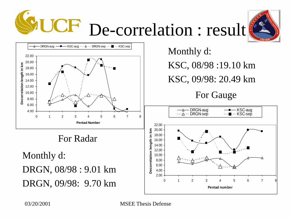
De-correlation : result

4.00

6.00

8.00

10.00

12.00

14.00

16.00

18.00

20.00

22.00

0 1 2 3 4 5 6 7 8

Pentad Number

De

co

rre

lati

on

le

ng

th in

km

DRGN-aug KSC-aug DRGN-sep KSC-sep

2.00

4.00

6.00

8.00

10.00

12.00

14.00

16.00

18.00

20.00

22.00

0 1 2 3 4 5 6 7 8

Pentad number

Deco

rrela

tio

n len

gth

in

km

DRGN-aug KSC-augDRGN-sep KSC-sep

For Radar

For Gauge

Monthly d:

KSC, 08/98 :19.10 km

KSC, 09/98: 20.49 km

Monthly d:

DRGN, 08/98 : 9.01 km

DRGN, 09/98: 9.70 km


x

x

xx

x

x

x

x

x

x

x

x

x

xx

2 km

2 km

DRGN Sub Areas


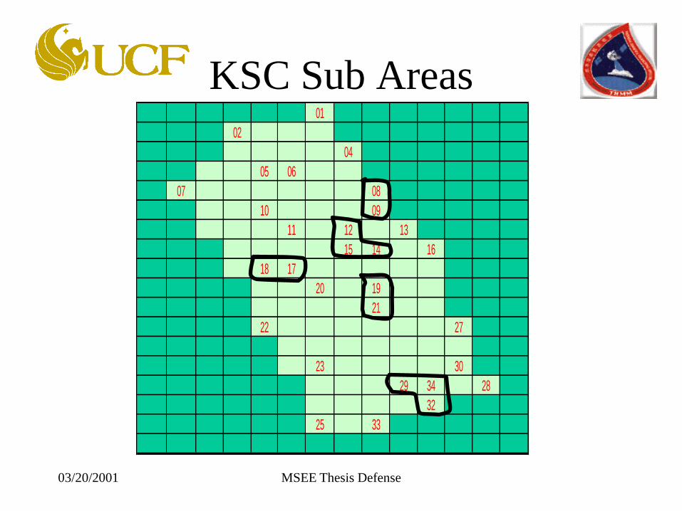
KSC Sub Areas01

02

04

05 06

07 08

10 09

11 12 13

15 14 16

18 17

20 19

21

22 27

23 30

29 34 28

32

25 33


Sub-network scale variation

-600

-400

-200

0

200

400

D1 D2 101C 112C 108C

Area labels

Vara

nce a

xis

-60

-40

-20

0

Mean

Axis

Diff. Variance Diff. Mean

-12000

-10000

-8000

-6000

-4000

-2000

0

K1 K2 K3 K4 K5

Area labels

Vara

nce a

xis

-100

-75

-50

-25

0

25

Mean

Axis

Diff. Variance Diff. Mean

DRGN

08/98

KSC

08/98


Contribution of area-point difference

to R-G difference variance

Table 3.7 Percentage contribution of area-point difference to R-G difference variance

Whole

NetworkD1 D2 101C 112C 108C

P1 18.84 10.74 9.07 11.06 11.06 11.06

P2 4.03 3.32 1.02 11.06 11.06 11.06

P3 14.72 8.11 18.01 11.06 11.06 11.06

P4 4.66 9.34 14.88 11.06 11.06 11.06

P5 2.54 9.02 5.57 11.06 11.06 11.06

P6 22.48 8.83 10.11 X 11.06 11.06

P7 10.79 12.67 0.48 11.06 11.06 X


Redundancy required?Month Cluster # R in mm Gauge ID G in mm

Aug-98 101C 132.14 101a 173.90

102 140.10

103 165.20

101b 186.50

112C 106.93 112 146.00

114 157.50

115 152.90

108C 170.65 108a 220.80

108b 207.30

108c 205.90

Sep-98 101C 150.53 101a 165.50

102 175.50

103 6.40

101b 164.10

112C 171.75 112 165.80

114 175.30

115 172.30

108C 138.13 108a 143.60

108b 14.50

108c 123.50

Site Radar

Estimate

Gauge ID Gauge

Estimate

R-G Average

R-G

Variance(G)

207 257.90 -4.06

312 268.80 -14.96

313 257.10 -3.26

314 250.20 3.64

315 24.50 229.34

Roi

Namur

253.84

316 257.20 -3.36

34.56 9141.46

208 59.90 120.86Illegini 180.76

311 106.30 74.46

97.66 1076.48

209 4.60 179.96Legan 184.56

306 182.10 2.46

91.21 15753.13

102 0.00 401.52RMI 102 401.52

111 361.20 40.32

220.92 65232.72

TEFLUN-B KWAJEX


Spatial Matching• Used a sliding window

method.

•Three different

Smoothing, namely, quad

smoothing, median filter

and trimming filter, is

used.

•Lagrange Polynomial

interpolation is also used:

magnification effect.

• A five point evaluation of

each method is carried out.


Quad Smoothing (QS)

P7 P8 P8 P9

P6P4

P1 P2 P3P2

P4 P6PC

PC

PC

PC

Quad 4

Quad 2

Quad 3

Quad 1

PC

1/20 2/20 1/20

2/20 8/20 2/20

1/20 2/20 1/20


Median and Trimming

• Median Filter (MF): Substitute the central

pixel value by the median of the 9 pixel

values.

• Trimming Filter: (TF)

– Sort the 9 values.

– Trim the two highest and 2 lowest values.

– average the the central subset of five elements.

– Substitute the central pixel by this average.


Interpolation method

Lagrange polynomial (LP) interpolation in two dimension

First interpolate along x:

Ii(x,yi)= nR(xn, yi )*Ln(x) ;

Ln(x) =[mn(x-xm)]/[mn(xn-xm)];

Next interpolate along y:

R(x,y)= iI(x, yi )*Li(y) ;

Li(x) =[mi(y-ym)]/[mi(yi-ym)];


Evaluation Criterion

• Probability of yielding better match.

• Difference of mean between radar and gauge.

• Difference in variance between radar and gauge.

• Average R/G over each network.

• Bulk R/G with all networks.

Result: The LP Method is giving best comparison


Improvement in KWAJTable 4.3 Comparison of bulk radar to gauge monthly estimates for KWAJ using quality

gauge data

Month Bulk G Bulk R from

‘O’

Bulk R from

‘LP’

O/G LP/G

08/1998 251.18 212.08 222.42 0.84 0.89

09/1998 344.68 325.98 327.65 0.95 0.95

11/1998 447.29 367.40 362.80 0.82 0.81

06/1999 295.91 364.43 346.12 1.23 1.17

07/1999 767.57 718.01 784.33 0.94 1.02

08/1999 1086.96 1069.72 1070.18 0.98 0.98

09/1999 899.45 720.80 742.58 0.80 0.83


TEFLUN-B Master GV Site• Located Approximately at 28.13N, 81.01W in the DRGN NETWORK

at Triple-N Ranch, Holopaw, Florida. Also called the 101 Gauge site.

• Relative arrangements of other instruments that are being compared

with gauge and NEXRAD are shown below.

101G101BG

UHF Profiler Assembly

Joss-Waldvogel

Disdrometer

2D Video

Disdrometer


Reflectivity time series

Reflectivity time series for J-Day 246, 1998

-10.000

0.000

10.000

20.000

30.000

40.000

50.000

60.000

17:30 17:44 17:58 18:13 18:27 18:42

Time in hh:mm

Refle

ctiv

ity in

dB

Z

2D JW Radar UHF

Reflectivity time series for J-Day 250, 1998

0

5

10

15

20

25

30

35

40

45

50

19:10 19:38 20:07 20:36 21:05 21:34 22:02

Time in hh:mm

Re

fle

cti

vit

y i

n d

BZ

2D Radar JW UHF


Rain rate time series

Sep 07, 1998 ( J-Day 250) Rain rate time series

-5

0

5

10

15

20

25

30

35

19:10 19:38 20:07 20:36 21:05 21:34 22:02

Time in hh:mm

Ra

in r

ate

in

mm

/h

G-101 G-101B 2D Radar JW

Sep 03, 1998 ( J-Day 246) Rain rate time series

-10

0

10

20

30

40

50

60

70

17:30 17:44 17:58 18:13 18:27 18:42

Time in hh:mm

Ra

in r

ate

in

mm

/h

G-101 G-101B 2D JW Radar


Temporal matching

• Three Methods examined:

– Resample all surface observation at radar VOS

time.

– Average the surface observation in a five

minute window around radar VOS time.

– Take median of the five minute window around

radar VOS time.


Evaluation

• Statistical significance test for mean and

variance are carried out to characterize

better matching of radar to surface.

• Other three factors for evaluation are:

– Correlation between two sets of estimate.

– Difference of Mean.

– Difference of variance.

Result: The Median Filter yields best comparison.


Result of combined spatial-temporal

filteringDifference in reflectivity before filtering

-30

-20

-10

0

10

20

30

40

50

17:32

17:36

17:42

17:47

17:52

17:57

18:02

18:07

18:12

18:17

18:22

18:32

18:37

18:42

Time in UTC

Dif

feren

ce i

n d

BZ

R-2D R-JWD R-UHF

Difference in reflectivity after filtering

-40

-30

-20

-10

0

10

20

30

40

50

17:32

17:36

17:42

17:47

17:52

17:57

18:02

18:07

18:12

18:17

18:22

18:32

18:37

18:42

Time in UTC

Dif

feren

ce i

n r

efl

ecti

vit

y

in d

BZ

R-2D R-JWD R-UHF

Before After


Conclusions

Q. What is the observed spatial variability of

precipitation?

Ans.: The Spatial Variability depends upon

the type and duration of precipitation. It

varies from region to region and in monthly

time scale the de-correlation length is of the

order of 10-20 km.


Conclusions

Q. Does the Spatial Variability affects radar

rain retrieval?

Ans.: Yes.

Q. How does the point-area difference affect

radar calibration?

Ans.: From about 11% to as high as 19%


Conclusions

Q. Do we need dual Z-R?

Ans.: Depends on what product we are interested in.

For area average rainfall over a long time, both

single and dual Z-R will yield similar result.

Q. Is redundancy of gauge observation required

before calibration?

Ans.: Yes, the gauges frequently give erroneous

observations.


Conclusions

Q. What is the best matching method found?

Ans.:

Spatially- Interpolate the coarse resolution

data exactly over the finer resolution grid.

Temporally - apply median filter to the fine

resolution data with a five minute window

centered around the coarse observation grid.


Usefulness

• Can be used for any multi-sensor calibration

/validation studies.


Related Publications

Documents

Spatial Variability of Surface Rainfall and its Impact on ... Variability of Surface Rainfall and its Impact on Radar Retrieval by ... Organization of the Thesis Chapter 1 ... I II