SPATIAL DATA ANALYSIS

Tony E. SmithUniversity of Pennsylvania

• Point Pattern Analysis

• Spatial Regression Analysis

• Continuous Pattern Analysis

POINT PATTERN ANALYSIS

Example Application Areas

• Housing Sales

• Crime Incidents

• Infectious Diseases

Philadelphia Pneumonia Example

!

!!

!

!

!

!

!

!!

!

!

!

!

!

!

!

!

!

!

!

!

!

!

!

!

!

!

!!

!

!

!

!

!

!

!

!!

!

!

!

! !

!

!

!

!

!

!

!!

!

!

!

!

!

!

! !

!

! !

!

!

!

!!

!

!

!

!

!

!

!

!

!

!

!

!

!

!

!

!

!

!

!

!

!

!

!!

!

!

!

!

!

!

!

!!

!

!

!

!

!

!

!

! !

!!

!

!

!

!

!

!

!

!

!

!

!

! !

!!

!

!

!

!

!

!

!

!!

!

!

!

!

!

!!

!

!

!

!

!

!

!

!

!

!

!

!

!

!

!

!

!

!

!!

!

!

!

!

!

!

!

!!

!

!

!

! !

!

!

!

!

!

!

!!

!

!

!

!

!

!

! !

!

! !

!

!

!

!!

!

!

!

!

!

!

!

!

!

!

!

!

!

!

!

!

!

!

!

!

!

!

!!

!

!

!

!

!

!

!

!!

!

!

!

!

!

!

!

! !

!!

!

!

!

!

!

!

!

!

!

!

!

! !

!!

!

!

!

!

!

!

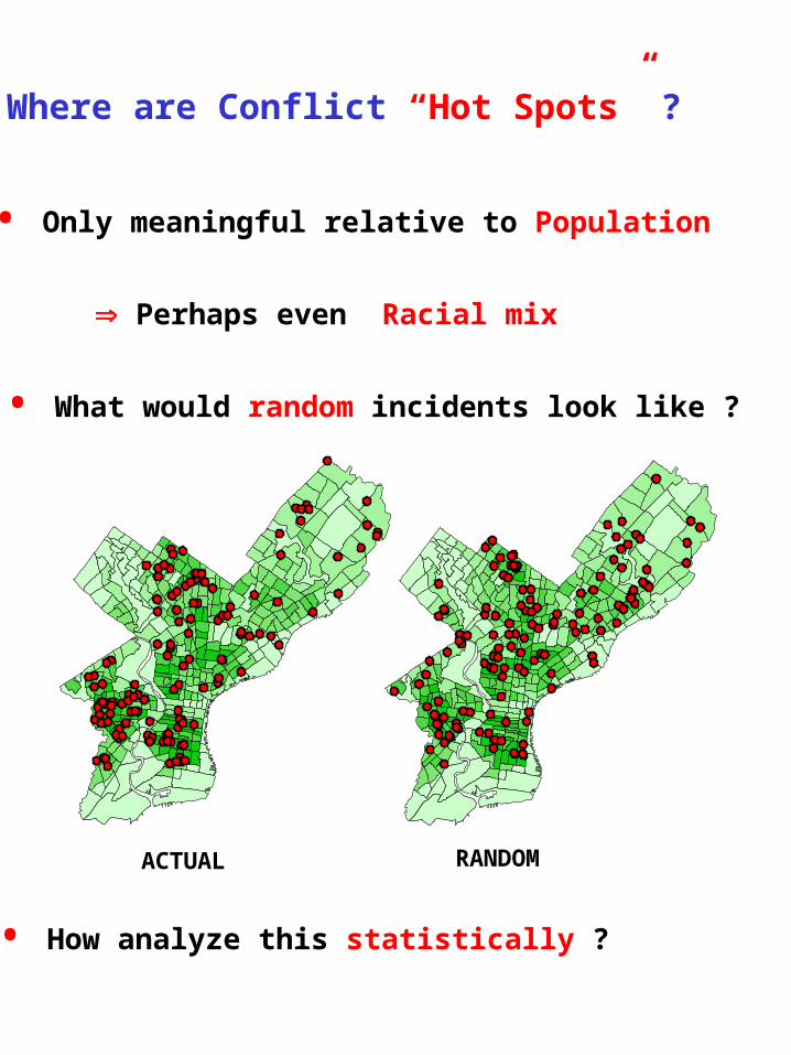
Where are Conflict “Hot Spots” ?

• Only meaningful relative to Population

Perhaps even Racial mix

• What would random incidents look like ?

• How analyze this statistically ?

ACTUAL RANDOM

!

!!

!

!

!

!

!

!!

!

!

!

!

!

!

!

!

!

!

!

!

!

!

!

!

!

!

!!

!

!

!

!

!

!

!

!!

!

!

!

! !

!

!

!

!

!

!

!!

!

!

!

!

!

!

! !

!

! !

!

!

!

!!

!

!

!

!

!

!

!

!

!

!

!

!

!

!

!

!

!

!

!

!

!

!

!!

!

!

!

!

!

!

!

!!

!

!

!

!

!

!

!

! !

!!

!

!

!

!

!

!

!

!

!

!

!

! !

!!

!

!

!

!

!

!

!

!!

!!

!

!

!!!!

!!!!

!

!

!!!

!! !!! !

! !!! !!

!!!! ! !!

! !!!

! !!

!!! !

! !! !

!!! !

!!!

!!

!!

!! !

! !! ! !

!!!!

!!

! !! !!

!! !!!

!!!! !

!!

! !!

!!!!

! ! ! !!!! ! !!!!! !!! ! !!!! ! ! !

! !!! !!

!

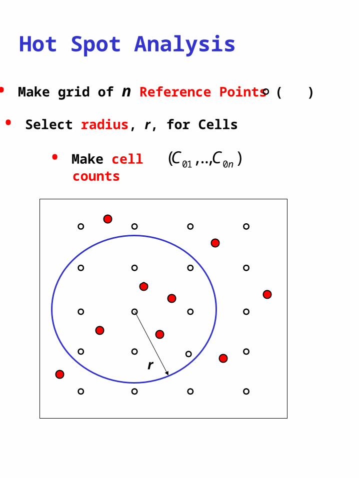
Hot Spot Analysis

• Make grid of n Reference Points ( )

• Select radius, r, for Cells

• Make cell counts

°

°

°

°

°

°

°

°

°

°

°

°

°

°

°

°

°

°

°

°

°

01 0( ,.., )nC C

r

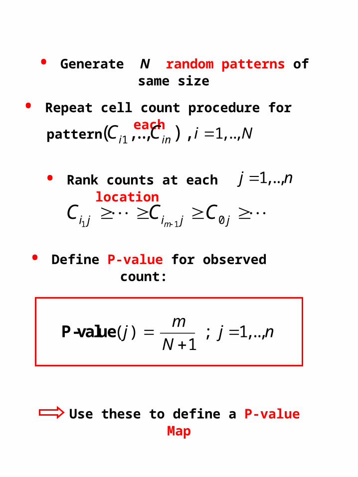
• Generate N random patterns of same size

• Repeat cell count procedure for each

1 1, ..,( ,.., ) ,i in i NC C pattern

• Rank counts at each location 1,..,j n

• Define P-value for observed count:

( ) ; 1,..,1

mj j n

N

P-value

1 1 0mi j i j jC C C

Use these to define a P-value Map

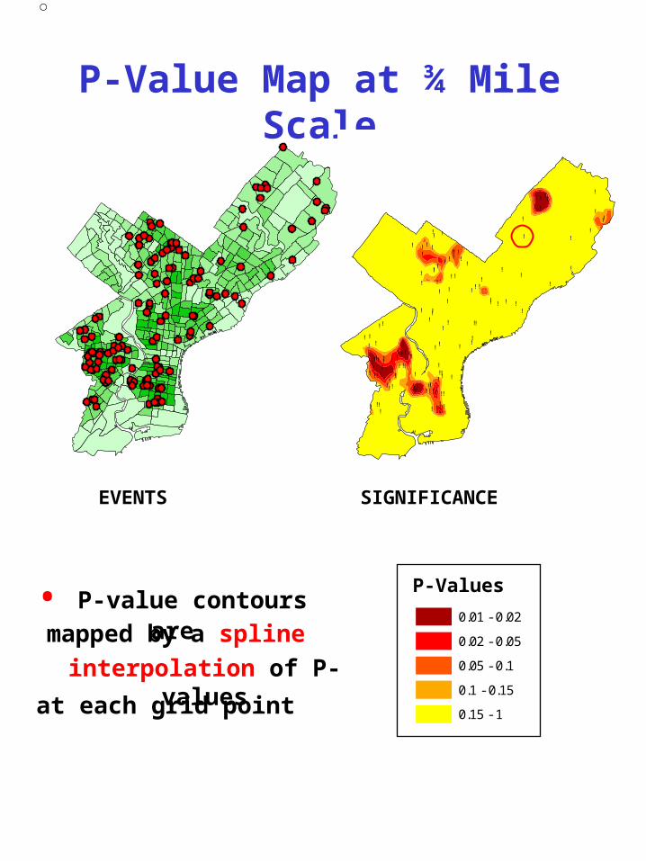
P-Value Map at ¾ Mile Scale

• P-value contours are

mapped by a spline

interpolation of P-values

at each grid point

Legend

mask_1

! Geocoding_Philadelphia

PVals at 3/4 miles

Prediction Map

[PVals].[D_015]

Filled Contours

0.01 - 0.02

0.02 - 0.05

0.05 - 0.1

0.1 - 0.15

0.15 - 1

P-Values

EVENTS SIGNIFICANCE

!

!!

!

!

!

!

!

!!

!

!

!

!

!

!

!

!

!

!

!

!

!

!

!

!

!

!

!!

!

!

!

!

!

!

!

!

!

!

!

!

! !

!

!

!

!

!

!

!!

!

!

!

!

!

!

! !

!

! !

!

!

!

!!

!

!

!

!

!

!

!

!

!

!

!

!

!

!

!

!

!

!

!

!

!

!

!!

!

!

!

!

!

!

!

!!

!

!

!

!

!

!

!

! !

!!

!

!

!

!

!

!

!

!

!

!

!

! !

!

!

!

!

!

!

!

!

!

!!

!

!

!

!

!

!!

!

!

!

!

!

!

!

!

!

!

!

!

!

!

!

!

!

!

!!

!

!

!

!

!

!

!

!!

!

!

!

! !

!

!

!

!

!

!

!!

!

!

!

!

!

!

! !

!

! !

!

!

!

!!

!

!

!

!

!

!

!

!

!

!

!

!

!

!

!

!

!

!

!

!

!

!

!!

!

!

!

!

!

!

!

!!

!

!

!

!

!

!

!

! !

!!

!

!

!

!

!

!

!

!

!

!

!

! !

!!

!

!

!

!

!

!

SPATIAL REGRESSION ANALYSIS

Example Applications

• Urban Area Data by:

• census tracts

• National Area Data by:

• block groups

• states

• counties

Ohio Lung Cancer Example

!(

!(

!(

!(

!(

!(

Akron

Dayton

Toledo

Columbus

Cleveland

Cincinnati

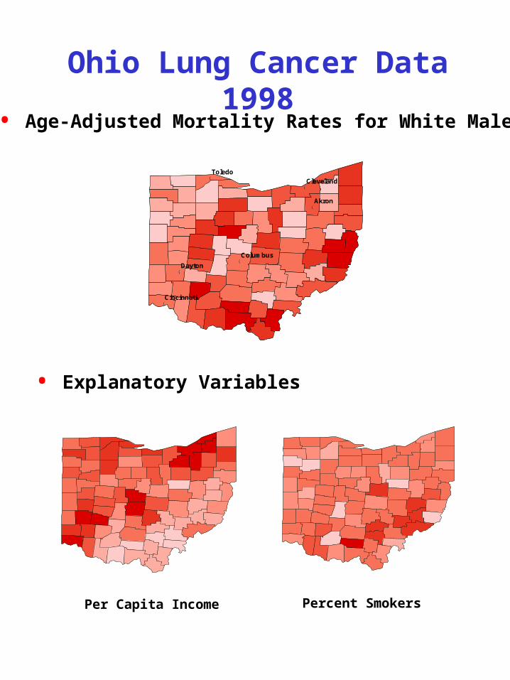
Ohio Lung Cancer Data 1998

• Age-Adjusted Mortality Rates for White Males

• Explanatory Variables

!(

!(

!(

!(

!(

!(

Akron

Dayton

Toledo

Columbus

Cleveland

Cincinnati

Per Capita Income Percent Smokers

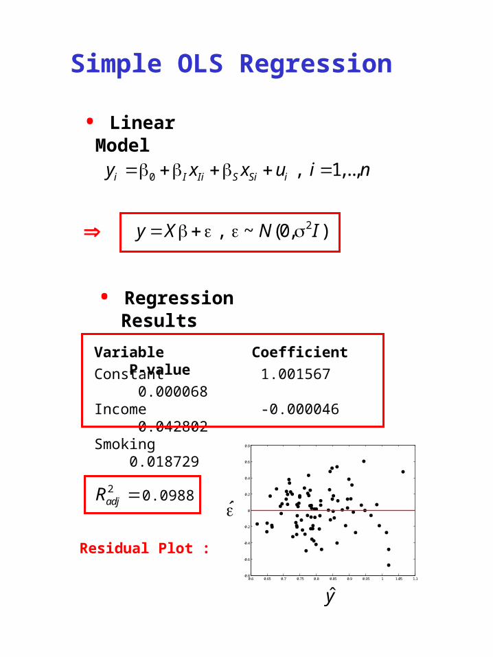
Simple OLS Regression

• Linear Model

0 , 1,..,i I Ii S Si iy x x u i n

2, ~ (0, )y X N I

• Regression Results

Variable Coefficient P-value

Constant 1.001567 0.000068 Income -0.000046 0.042802 Smoking 0.942823 0.018729

0.09882adjR

Residual Plot :

y0.6 0.65 0.7 0.75 0.8 0.85 0.9 0.95 1 1.05 1.1

-0.8

-0.6

-0.4

-0.2

0

0.2

0.4

0.6

0.8

Spatial Autocorrelation Problem

• One-Dimensional Example

••• •• •

•••

TRUE TREND

y

x

••• •• •

•••

TRUE TREND

y

x

REGRESSION LINE

Correlated Errors

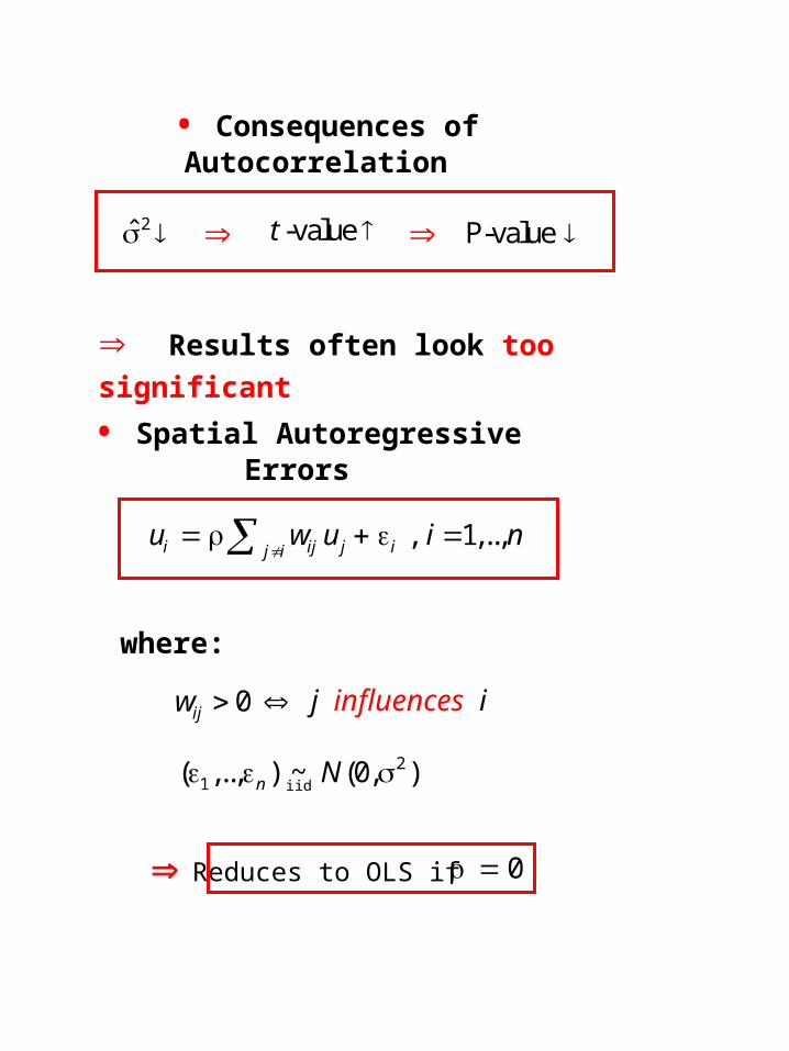
• Consequences of Autocorrelation

2 -valuet P-value

• Spatial Autoregressive Errors

Results often look too significant

, 1,..,i ij j ij iu w u i n

where:

0ijw j influences i

21( ,.., ) ~ (0, )n N

iid

Reduces to OLS if 0

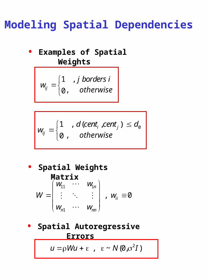
Modeling Spatial Dependencies

• Examples of Spatial Weights

1 ,

0ij

j borders iw

, otherwise

01 , ( , )

0i j

ij

d cent cent dw

, otherwise

• Spatial Weights Matrix

11 1

1

, 0n

ii

n nn

w w

W w

w w

• Spatial Autoregressive Errors

2, ~ (0, )u Wu N I

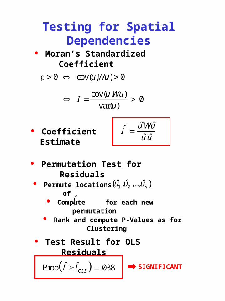
Testing for Spatial Dependencies

• Moran’s Standardized Coefficient

0 cov( , ) 0u Wu

cov( , )0

var( )

u WuI

u

• Coefficient Estimateˆ ˆˆ ˆ ˆ

u WuI

u u

• Permutation Test for Residuals

• Permute locations of 1 2ˆ ˆ ˆ( , ,.., )nu u u

• Compute for each new permutation I

• Rank and compute P-Values as for Clustering

• Test Result for OLS Residuals

ˆ ˆProb .038OLSI I SIGNIFICANT

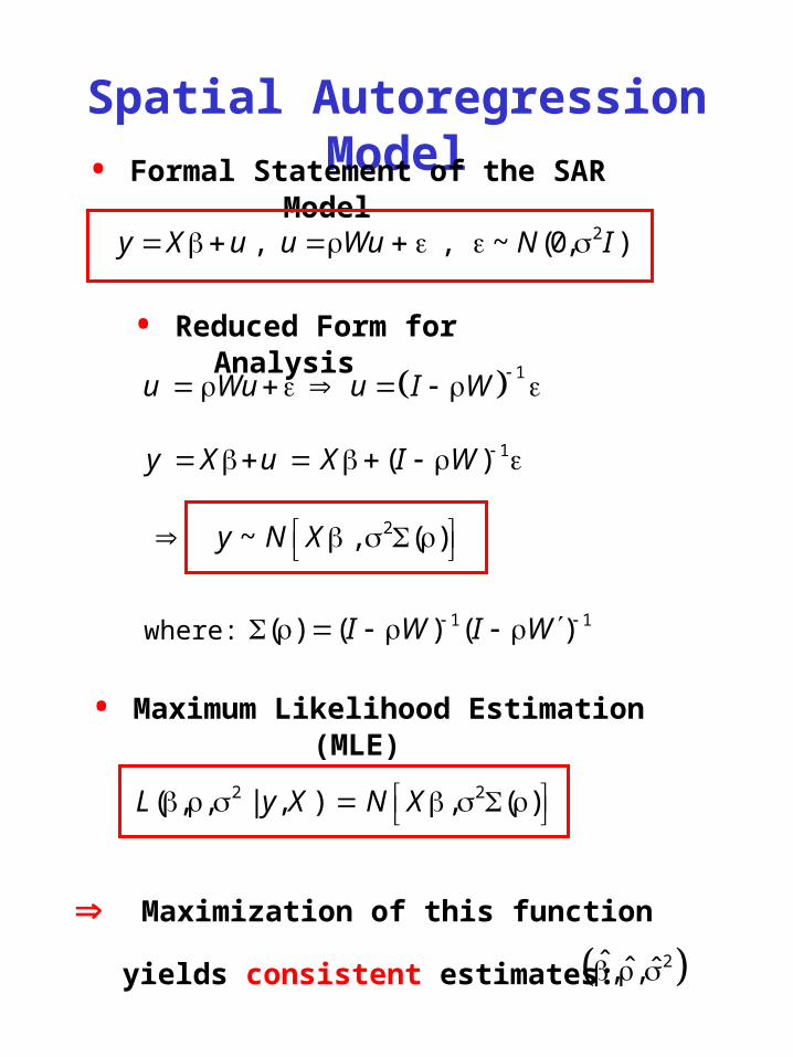
Spatial Autoregression Model

• Reduced Form for Analysis

1u Wu u I W

1( )y X u X I W

• Maximum Likelihood Estimation (MLE)

where: 1 1( ) ( ) ( )I W I W

2~ , ( )y N X

yields consistent estimates:

Maximization of this function

2ˆ ˆ ˆ, ,

2 2( , , | , ) , ( )L y X N X

• Formal Statement of the SAR Model

2, , ~ (0, )y X u u Wu N I

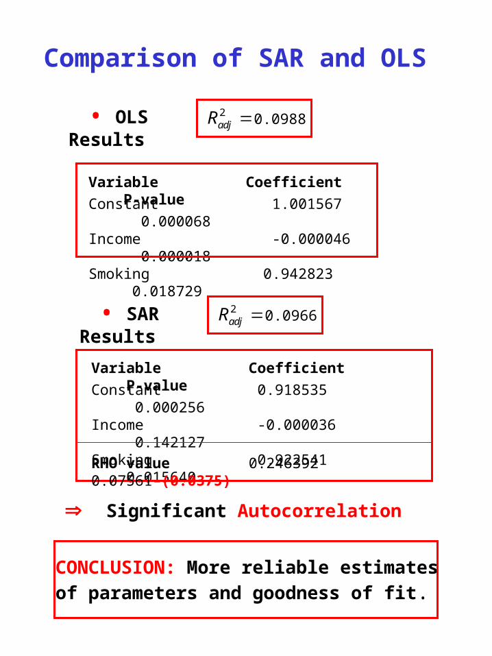
Comparison of SAR and OLS

• OLS Results

Variable Coefficient P-value

Constant 1.001567 0.000068 Income -0.000046 0.000018 Smoking 0.942823 0.018729

0.09882adjR

Variable Coefficient P-value

Constant 0.918535 0.000256 Income -0.000036 0.142127 Smoking 0.922541 0.015640

0.09662adjR • SAR Results

Significant Autocorrelation

RHO value 0.246392 0.07561 (0.0375)

CONCLUSION: More reliable estimates

of parameters and goodness of fit.

CONTINUOUS PATTERN ANALYSIS

Example Application Areas

• Weather Patterns

• Mineral Exploration

• Environmental Pollution

• Geologic Analyses

Venice Example

INDUSTRY

VENICE

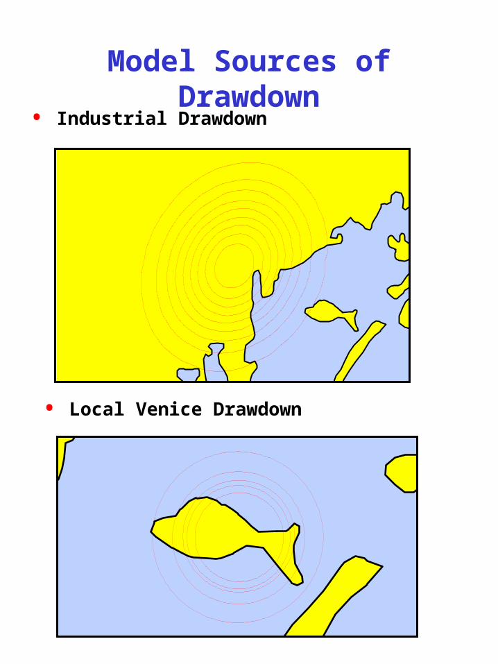
Model Sources of Drawdown

• Industrial Drawdown

• Local Venice Drawdown

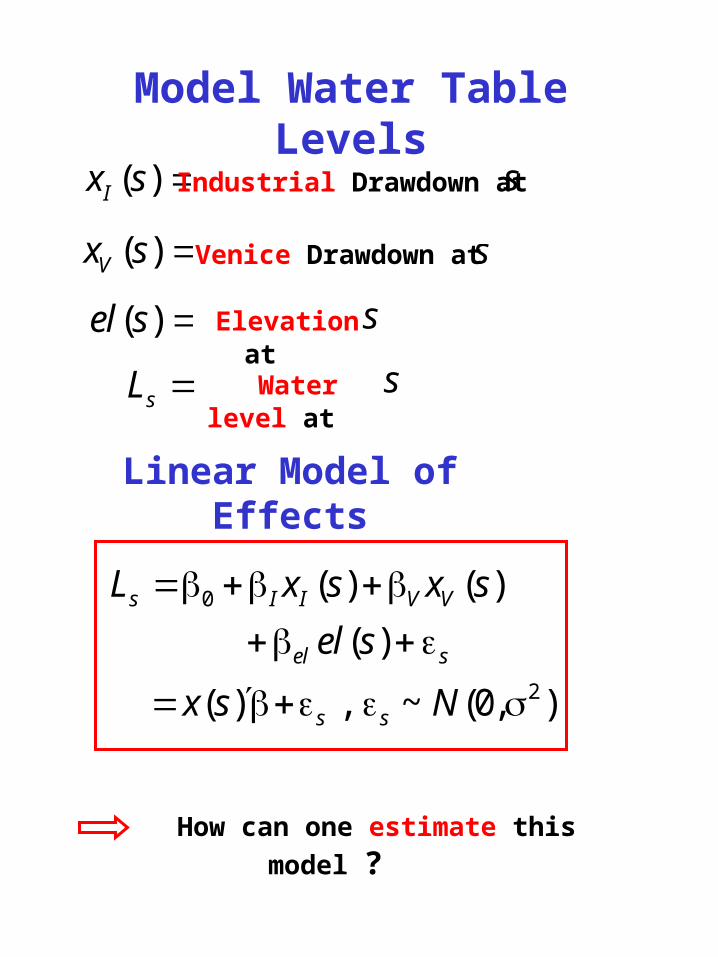
Model Water Table Levels

( )Ix s

( )Vx s

Industrial Drawdown at

Venice Drawdown at

s

s

( )el s Elevation at s

sL Water level at s

Linear Model of Effects

0

2

( ) ( )

( )

( ) , ~ (0, )

s I I V V

el s

s s

L x s x s

el s

x s N

How can one estimate this model ?

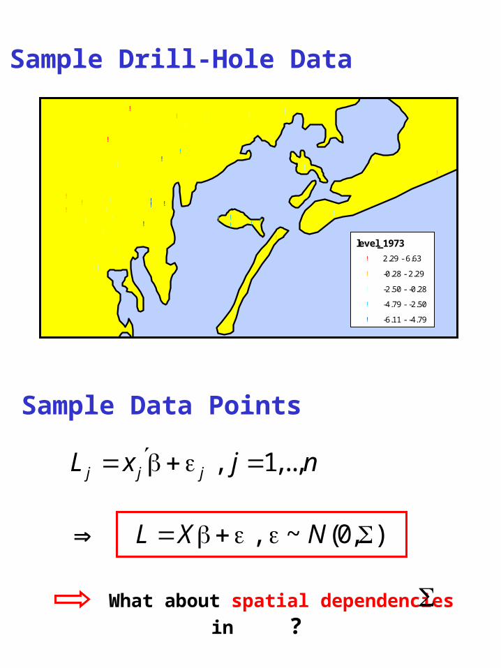
Sample Drill-Hole Data

Sample Data Points

, 1,..,j j jL x j n

, ~ (0, )L X N

What about spatial dependencies in ?

!

!!

!

!

!

!!

!

!

!

!

!

!

!

!

!! !

!

!

!!

!

!

!!

!

!

!!

!

!

!

!

!

!

!!! Legend

level_1973

! 2.29 - 6.63

! -0.28 - 2.29

! -2.50 - -0.28

! -4.79 - -2.50

! -6.11 - -4.79

Coastline

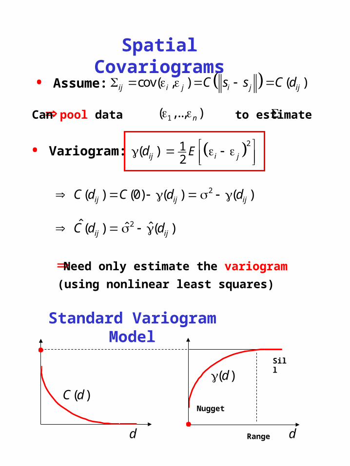
Spatial Covariograms

• Assume: cov( , ) ( )ij i j i j ijC s s C d

• Variogram:

Can pool data to estimate

212

( )ij i jEd

2( ) (0) ( ) ( )ij ij ijC d C d d

2ˆ ˆˆ( ) ( )ij ijC d d

Need only estimate the variogram

Standard Variogram Model

Sill

Nugget

Ranged d

( )C d

( )d

(using nonlinear least squares)

1( ,.., )n

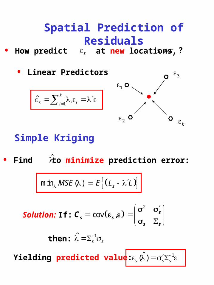
Spatial Prediction of Residuals

• How predict at new locations,s js s ?

1

2

3

k

• Linear Predictors

1ˆ

k

s i ii

Simple Kriging

• Find to minimize prediction error:

Solution: If:

min ( ) sMSE E L L

2

cov ,

s

s s

s s

C

then: 1ˆs s

Yielding predicted value: 1ˆ( )s s s

• Given linear model , ~ (0, )L X N

to obtain consistent estimates:

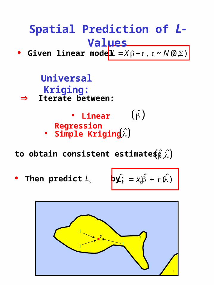
Spatial Prediction of L-Values

Iterate between:

• Linear Regression

• Simple Kriging

Universal Kriging:

ˆ ˆ,

• Then predict by:sL ˆ ˆˆ ( )s sL x

•

!!

!

!

!!!

s•

Results for Venice:

Can be 95% confident that each meter of

industrial drawdown lowers the Venice

water table by at least at least 15 cm.

• Predicted Water Table Levels

• Analysis for Policy Conclusions

ACTION: Drawdown was restricted (1973)

RESULT: Venice elevation increased (1976)