Agribusiness and Applied Economics Report No. 604 May 2007

Spatial Competition and Ethanol Plant Location Decisions

Camilo Sarmiento and William W. Wilson

Department of Agribusiness and Applied Economics

Agricultural Experiment Station North Dakota State University

Fargo, ND 58105-5636

Acknowledgments Thanks are given to Edie Nelson for document preparation and to Cole Gustafson, Won Koo and Dragan Miljkovic for reviewing this manuscript. We would be happy to provide a single copy of this publication free of charge. You can address your inquiry to: Department of Agribusiness and Applied Economics, North Dakota State University, P.O. Box 5636, Fargo, ND, 58105-5636, Ph. 701-231-7441, Fax 701-231-7400, e-mail ndsu.agribusiness@ndsu.edu. This publication is also available electronically at: http://agecon.lib.umn.edu/. NDSU is an equal opportunity institution. Copyright© 2007 by William W. Wilson. All rights reserved. Readers may make verbatim copies of this document for non-commercial purposes by any means, provided this copyright notice appears on all such copies.

i

Table of Contents

List of Tables .................................................................................................................................. ii

List of Figures ................................................................................................................................. ii

Abstract .......................................................................................................................................... iii

Introduction ......................................................................................................................................1

Development of the U.S. Ethanol Industry ......................................................................................2

Empirical Analysis of Ethanol Plant Location .................................................................................4 Model Specification .............................................................................................................4 Econometric Model ..............................................................................................................5 Explanatory Variables Spatial Effects .................................................................................7 Data ......................................................................................................................................7 Estimation ............................................................................................................................8

Analysis of Results ..........................................................................................................................9 Econometric Results ............................................................................................................9 Interpretation of Probabilities ............................................................................................13

Summary and Implications ............................................................................................................14

References ......................................................................................................................................16

ii

List of Tables

Table 1 .............................................................................................................................................9

Table 2 ...........................................................................................................................................10

List of Figures

Figure 1 ..........................................................................................................................................11

Figure 2 ..........................................................................................................................................12

Figure 3 ..........................................................................................................................................13

iii

Abstract Ethanol is one of the fastest growing industries in the U.S. agricultural sector. This study

estimates factors that impact location decisions by new ethanol plants using logistic regression

analysis and spatial correlation techniques. The results indicate that location decisions are

impacted by the agricultural characteristics of a county, competition, and state-level subsidies.

Spatial competition is particularly important. Existence of a competing ethanol plant reduces the

likelihood of making a positive location decision and this impact decreases with distance.

Finally, state-level subsidies were significant and a very important variable impacting ethanol

location decisions.

Key Words: Ethanol, Spatial Autocorrelation, Location Decision

1

Spatial Competition and Ethanol Plant Location Decisions

Camilo Sarmiento and William W. Wilson∗

Introduction

One of the most dramatic changes in agriculture in recent decades is that related to ethanol. These are driven in part by federal and state mandates and subsidies, but are also impacted by technology and the dynamics of the world and the U.S. oil and energy sectors. Indeed, investment in this sector is resulting in one of the most important changes in agriculture in recent decades. Finally, ethanol provides a new form of value-added agriculture, there is intense interstate competition, as well as local competition to influence ethanol plant location decisions. 1 Corn is the primary feedstock for U.S. ethanol production. In 2007, corn planted decisions reached its highest level since 1944, primarily in response to the growing demand for ethanol.2 Proximity of ethanol plants to grain production is thus an important component of plant location.

The purpose of this paper is to analyze factors that impact location decisions for ethanol

plants. Specifically, we examine impacts of agricultural characteristics of counties, as well as the spatial dimensions of competition and state subsidies on ethanol plant location decisions. The econometric analysis follows the Sarmiento and Wilson (2005) model of discrete spatial competition (McMillan 1995) and builds on other recent studies using spatial autocorrelation to analyze spatial competition (Anselin 2003; Irwin and Bockstael 2003; Anselin, Bongiovanni, and Lowenberg-DeBoer 2004; McMillan 1995; Nelson 2002; Nelson and Geoghegan 2002).

We estimate the effect of agricultural characteristics, state subsidies, and industrial spatial

competition on ethanol plant location. The analysis tackles the question of how geographical proximity to other plants impacts ethanol plant location decisions. It also explores the hypothesis of whether competition increases or hinders local investment in new plants. Results underscore the importance of agricultural characteristics of the county in explaining ethanol plant location. Acreage planted to corn and other crops, as well as corn demand for uses different ∗ Sarmiento is Senior Economist, Business Analytics and Decisions, Fannie Mae, Washington, DC, and Wilson is professor, Department of Agribusiness and Applied Economics, North Dakota State University, Fargo 1 Issues related to ethanol have also become topics in some of the more popular business press. Business Week (August 14, 2006, p. 56) noted “Facilities that can turn kernels into clean fuel seem to be sprouting up faster than the corn itself. There are 101 ethanol plants in existence, more than 42 new facilities and expansions in the works, and another 100 in the planning stages....Investors are wowed by the combination of short supply, surging demand, and government subsidies that top $2 billion annually (Green 2006). And, in a recent Fortune article (Brown 2006), it was indicated that Iowa had 25 ethanol plants operating, four are under construction and another 26 are planned, and indicated (citing Wisener) “if all those plants are built, distilleries would use the entire Iowa corn harvest. Finally, Hurd indicated “There is a ‘gold rush’ occurring now in building ethanol plants” (as reported by Wulf 2006).

2 Ethanol can also be made from other products such as grain sorghum (milo), wheat, barley, sugar cane or beets, cheese whey, and potatoes.

2

from ethanol, are main components of plant location. We also examine the role of state subsidy incentives, which vary across states and are an important component of inter-state competition for value-added activities on ethanol plant location.

Overall, local competition reduces ethanol plant growth, but this effect is ameliorated by

the local agricultural characteristics and local government subsidies. After accounting for the characteristics of the county, we find that spatial competition amongst ethanol plants negatively impacts plant location decisions. Spatial relationships to corn production have a positive impact. This result contrasts with the role of competition on other high value investment decisions in agribusiness, e.g., development of shuttle train elevators (Sarmiento and Wilson, 2005).

Development of the U.S. Ethanol Industry

An important change in U.S. grain consumption is corn use for ethanol. This industry has

been expanding during the past decade, and its rate of expansion is expected to accelerate. Ethanol uses for automobile fuel date back to the beginning of the 20th century. Ethanol was used to fuel cars in the 1920s and 1930s. By the 1940s, however, use of agricultural crops to produce liquid fuels had dissipated. Fuels from petroleum and natural gas became available in large quantities at low cost, eliminating the economic incentives for production of liquid fuels from crops.

The oil crises of the 1970s renewed interest in ethanol. Ethanol was blended directly into

gasoline in a mix of 10% ethanol and 90% gasoline, called gasohol. In 1978, Congress approved the National Energy Act, which included a Federal tax exemption for gasoline containing 10% alcohol. The Federal subsidy reduced the cost of ethanol to near the wholesale price of gasoline, making it economically viable as a gasoline blending component. The growth of ethanol is enhanced substantially by state tax incentives to ethanol producers. Federal and State tax incentives make ethanol economically attractive in the Midwest, but there are difficulties with the high cost of transporting ethanol to consumption markets.

In the 1990s, ethanol was perceived as a way to help farmers increase cash flows from

their corn crop. Growth of ethanol, however, stalled as prices of oil reached low levels in the 1990s and the increased demand for fuel from China and scarcities in production, as well as global concern on global warming, has provided renewed incentives for ethanol production. Indeed, in the last few years, ethanol production has grown rapidly. By the end of 2006, the ethanol industry reached a capacity of more than 6 billion gallons. Currently, there are 115 ethanol production facilities in the United States and 71 more are under construction.

For perspective on growth and changes in this sector, in 2003 indications were that the

corn demand for ethanol was projected to increase by one billion bushels in the next 10 years (Feltes 2003); the United States will need another 40 or 50 ethanol plants that would divert another one billion bushels of corn to match the same billion bushels devoted to ethanol production today (ProExporter 2004). And, “more than one billion bushels of corn will be used to produce ethanol in 2003/04, and this approaches two billion bushels by the end of the decade” [U.S. Department of Agriculture-Economic Research Service (USDA-ERS 2003)]. These

3

assertions were made prior to recent energy initiatives that would expand the future role of ethanol and biodiesel. The Energy Policy Act of 2005 established the Renewable Fuel Standards (RFS) at 4 billion gallons in 2006, increasing to 7.5 by 2012.

There are numerous aspects of the growth in demand for ethanol production. One is the

location of new ethanol plants.3 Though ethanol production was earlier concentrated in the Eastern Corn Belt, the recent expansions have concentrated in the Western Corn Belt which now has about 42% of the capacity. The Central Plains is the third largest region. Existing plants comprise about 6 billion gallons of capacity and, when taken together with planned plants, total capacity would be about 12 billion gallons.

Projections have changed recently on ethanol targets and mandates. Both the Energy

Information Administration’s (EIA) 2005 and 2006 reports make projections to 2015. The EIA 2005 projections were for ethanol from corn production at just less than four billion gallons. The EIA 2006 estimate expanded on this level to nearly 10 billion gallons in 2015, and then converges to about 11 billion gallons in 2020 forward. In the period after 2015, a minor portion of this will be met by ethanol from cellulose (EIA 2005). The 2007 State of the Union address suggested further expansion in this sector. These are fairly drastic changes. Demand growth should taper off beginning in about 2020. Ethanol consumption suggests the growth in demand for corn for ethanol to increase from about 1.4 billion bushels in 2005/2006 to about four billion bushels by 2020.

The principal byproduct from ethanol production is referred to as distillers’ dry grains

(DDGs). Wide-scale use of the byproduct is just evolving and there is much to be known about its feeding value and shipping characteristics. Some is exported, but this is limited due in part to its lower value and higher cost of shipping. The maximum amount that can be used in rations varies by animal type and herd competition. The rate of adoption of DDGs for corn is less than the rate of substitution in corn rations (i.e., a lot more corn could be displaced with wider adoption of DDGs for livestock ratios). The substitution rate of DDGs for corn in livestock is 40 lbs. of corn is displaced by 400 lbs. of DDGs; and for swine and poultry, 177 lbs. of corn is displaced by 200 lbs. of DDGs (Urbanchuk 2003). The effect of ethanol on Iowa indicated DDGs are largely fed to cattle and that swine and poultry are largely untapped markets (Otto and Gallagher 2003). 4

There are numerous issues and views on the prospects of there being enough corn to meet demands for both the growing world market and the U.S. ethanol market. ProExporter (2006b)

3 These plants and planned projects were taken from Renewable Fuels Association (April 2006). 4 For swine it is not so much a nutritional challenge as it is a carcass quality issue. At inclusion levels greater than 20% in grower/finisher diets, fat quality deteriorates (especially belly fat) which impacts carcass quality, leading to discounts. A positive for DDGs inclusion is that at 10% substitution (which has no negative impact on fat), the producer saves 178 lbs. of corn and 20 lbs. of soybeans, and can remove the dicalcium phosphate. These savings with current prices would be about $3.50/ton or perhaps $1.00 per pig.

4

estimated there were 5.3 billion gallons of capacity currently operating and another 6 billion under construction. In addition, they indicated there were an additional 369 projects on the drawing boards representing an additional 24.7 billion gallons of ethanol capacity (as reported in Mann Global Research, 2006c). They indicated the ethanol margin in 2005 was 152 c/bu of corn processed. This has declined to 44 c/bu this year, and was more than attractive to justify additional investment. In contrast, Goldman Sachs (as reported by Red River Farm Network, 2006) expressed worry about high corn prices, indicating that rising corn prices threaten profitability of ethanol. Biomargins have been hurt by a 55% increase in corn price and the price of ethanol has risen by 8%. Without producer incentives and tax credits, Goldman Sachs believes many biofuel plants would be unprofitable.

Finally, there is much debate and discussion about the response of U.S. agriculture to this

change in demand. One is the growth rate in yields and whether productivity increases will be adequate to support this industry (Schlicher 2006; Meyer 2006; Wisener and Hurd as reported by Smith 2006; Sosland Publishing 2006). A second area is the source of additional acres that could be shifted to corn. Most analysis suggests it will come from changes in rotations (Hart 2006b, Fatka 2006b), soybeans, and some from the CRP program (Fatka 2006a; Hart 2006a; Mann Global Research 2006c). However, the ability to shift CRP acres into corn acres is highly spatially dependent (Mann Global Research 2006c; Pates 2006). USDA’s Collins (2006) indicated that ethanol plants will be able to bid corn away from a variety of other uses and that the United States will need substantial increases in corn acreage to prevent reductions in exports. He also indicated “there could come a time in years ahead when U.S. agriculture may not be able to meet the increased needs of ethanol and biodiesel while continuing to supply feed needs of the poultry and livestock sectors” (Schuff 2006c, referring to testimony of processors to the House Agriculture Committee).

In summary, ethanol production is one of the most dramatic changes in U.S. agriculture

in many decades. There are several issues on the aggregate impacts of this industry on grain and agriculture. There are, no doubt, many proprietary studies being conducted on location decisions, but there are few published studies that analyze location decisions and factors that impact them. There are many issues related to these location decisions, including the role of corn supplies, competing crops, state subsidies, existence of competing plants, and the spatial interdependencies of all these variables.

Empirical Analysis of Ethanol Plant Location

Model Specification

We specify a discrete choice model for ethanol plant location. The choice variable is county location and the explanatory variables are factors that explain comparative advantages for the plant to locate in a given county. Payoffs for the ethanol plant to locate in county j, πj depends on agricultural characteristics of the county, spatial externalities from the county location, local users of ethanol byproducts, policy variables, and spatial competition.

5

These payoffs are more complicated due to the intermarket relationships and to uncertainties on each of the variables, particularly uncertainties of expectations of investors, as well as the intermarket competition amongst ethanol and DDGs shipments, and corn procurement. However, this is sufficient for our purposes. A condition for investing in an ethanol plant is that expected payoffs from ethanol must be at least as large as the payoffs from the alternative, πj ≥ πk, for j ≠ k. Thus, the condition for investing in an ethanol plant in location j is: (1) δj =1, if πj,k = ƒ(Xj) − ƒ(Xk) ≥ 0 for ∀j ≠ k; else δj =0. where πj = ƒ(Xj) and Xj are location factors related to plant j. From (1), the probability that an ethanol plant locates in county j is: (2) P(δj =1) = F(Xj, π-j), where π -j are payoffs to locations different from plant j.

In modeling the firm’s decision to invest in an ethanol plant at a given location, we observe the result of the plant investment decision in (1), but do not observe the value of alternative payoffs by location π-j. Payoffs at alternative locations can be captured with an index of competition from other ethanol plant locations, captured with a spatial lagged dependent variable. That is,

(3) P(δj =1) ≈ F(Xj, SL-j), where as in Sarmiento and Wilson (2005),

(4) SL-j = ∑≠ jk

Dkexp(−Distjk/γ),

where Dk = 1 if an ethanol plant locates in county k, and Dk = 0 else; and Distjk is the distance between plants j and k. Location factors in Xj, e.g., corn availability, may be further interrelated across counties and depend on the distance between plants. Econometric Model

From equation (3), the probability of building an ethanol plant in county j depends on payoffs from locating the plant in that county and spatial competition. We include agricultural characteristics for each county, policy variables, and firm competition as factors that determine payoffs from plant locating in county j.

Agricultural characteristics of the county include production and acreage planted of corn, as well as other grains (soybean, wheat, barley, sorghum, and sunflower). We use the Herfindahl

6

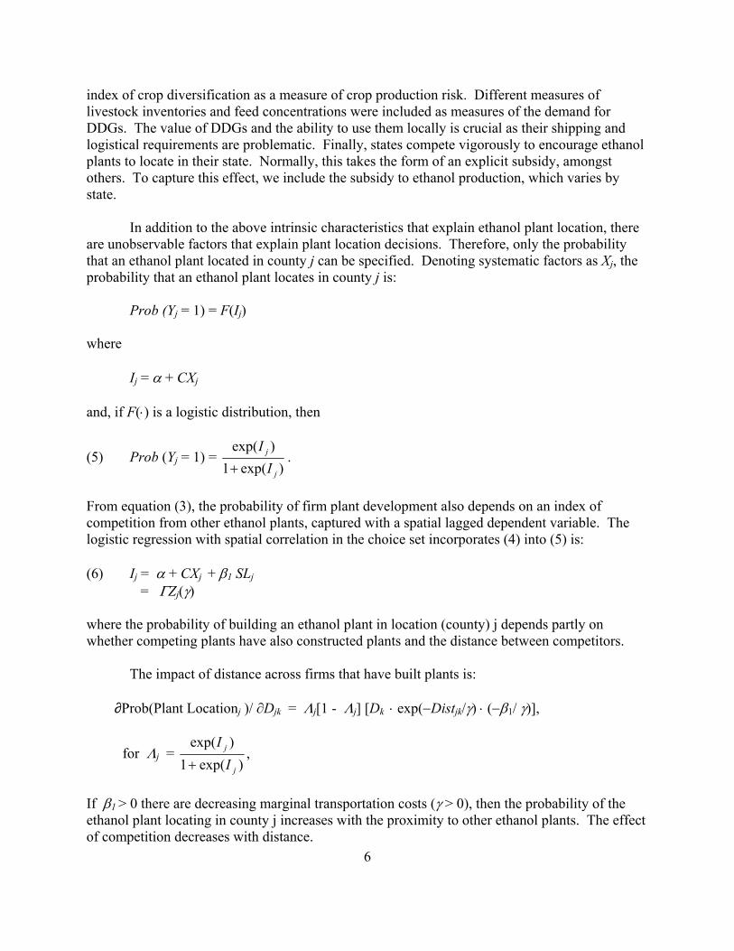
index of crop diversification as a measure of crop production risk. Different measures of livestock inventories and feed concentrations were included as measures of the demand for DDGs. The value of DDGs and the ability to use them locally is crucial as their shipping and logistical requirements are problematic. Finally, states compete vigorously to encourage ethanol plants to locate in their state. Normally, this takes the form of an explicit subsidy, amongst others. To capture this effect, we include the subsidy to ethanol production, which varies by state.

In addition to the above intrinsic characteristics that explain ethanol plant location, there are unobservable factors that explain plant location decisions. Therefore, only the probability that an ethanol plant located in county j can be specified. Denoting systematic factors as Xj, the probability that an ethanol plant locates in county j is:

Prob (Yj = 1) = F(Ij)

where Ij = α + CXj and, if F(⋅) is a logistic distribution, then

(5) Prob (Yj = 1) = )exp(1

)exp(

j

j

II

+.

From equation (3), the probability of firm plant development also depends on an index of competition from other ethanol plants, captured with a spatial lagged dependent variable. The logistic regression with spatial correlation in the choice set incorporates (4) into (5) is: (6) Ij = α + CXj + β1 SLj

= ΓZj(γ)

where the probability of building an ethanol plant in location (county) j depends partly on whether competing plants have also constructed plants and the distance between competitors.

The impact of distance across firms that have built plants is:

∂Prob(Plant Locationj )/ ∂Djk = Λj[1 - Λj] [Dk ⋅ exp(−Distjk/γ) ⋅ (−β1/ γ)],

for Λj = )exp(1

)exp(

j

j

II

+,

If β1 > 0 there are decreasing marginal transportation costs (γ > 0), then the probability of the ethanol plant locating in county j increases with the proximity to other ethanol plants. The effect of competition decreases with distance.

7

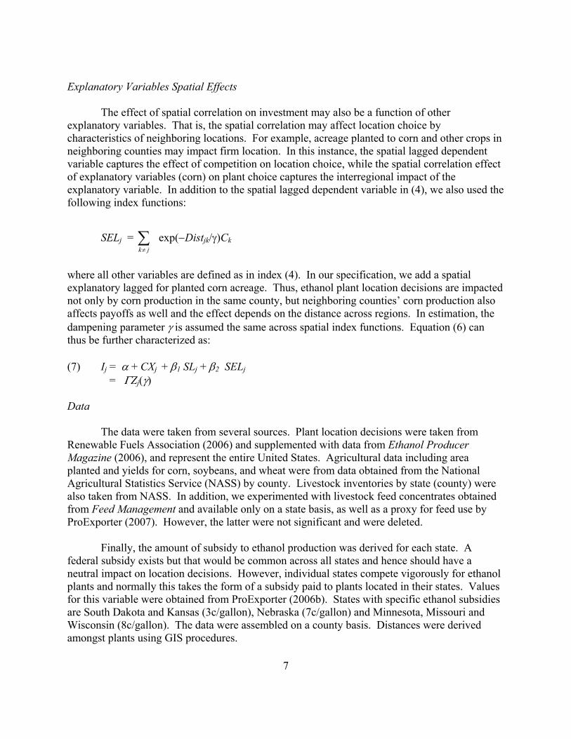
Explanatory Variables Spatial Effects The effect of spatial correlation on investment may also be a function of other explanatory variables. That is, the spatial correlation may affect location choice by characteristics of neighboring locations. For example, acreage planted to corn and other crops in neighboring counties may impact firm location. In this instance, the spatial lagged dependent variable captures the effect of competition on location choice, while the spatial correlation effect of explanatory variables (corn) on plant choice captures the interregional impact of the explanatory variable. In addition to the spatial lagged dependent variable in (4), we also used the following index functions:

SELj = ∑≠ jk

exp(−Distjk/γ)Ck

where all other variables are defined as in index (4). In our specification, we add a spatial explanatory lagged for planted corn acreage. Thus, ethanol plant location decisions are impacted not only by corn production in the same county, but neighboring counties’ corn production also affects payoffs as well and the effect depends on the distance across regions. In estimation, the dampening parameter γ is assumed the same across spatial index functions. Equation (6) can thus be further characterized as: (7) Ij = α + CXj + β1 SLj + β2 SELj

= ΓZj(γ)

Data The data were taken from several sources. Plant location decisions were taken from Renewable Fuels Association (2006) and supplemented with data from Ethanol Producer Magazine (2006), and represent the entire United States. Agricultural data including area planted and yields for corn, soybeans, and wheat were from data obtained from the National Agricultural Statistics Service (NASS) by county. Livestock inventories by state (county) were also taken from NASS. In addition, we experimented with livestock feed concentrates obtained from Feed Management and available only on a state basis, as well as a proxy for feed use by ProExporter (2007). However, the latter were not significant and were deleted. Finally, the amount of subsidy to ethanol production was derived for each state. A federal subsidy exists but that would be common across all states and hence should have a neutral impact on location decisions. However, individual states compete vigorously for ethanol plants and normally this takes the form of a subsidy paid to plants located in their states. Values for this variable were obtained from ProExporter (2006b). States with specific ethanol subsidies are South Dakota and Kansas (3c/gallon), Nebraska (7c/gallon) and Minnesota, Missouri and Wisconsin (8c/gallon). The data were assembled on a county basis. Distances were derived amongst plants using GIS procedures.

8

Estimation

Distance in the spatial indexes in (7) of the discrete choice model with spatial correlation enters non-linearly because of uneven frequencies when defining lags in a spatial framework. Available software designed to estimate dichotomous choice models with spatial correlation data is not readily available. We thus developed a procedure to estimate the discrete choice of plant location with an algorithm that converges easily. To do so, we concentrate the logistic likelihood function in terms of the non-linear coefficient in the spatial correlation function (Sarmiento and Wilson 2005; Sarmiento and Wilson 2007). In particular, the estimator of (5) with the index function in (7) is obtained by solving the optimization:

(8)

γMax lnL(γ)

s.t. Σi(yi − Λi)Zi(γ) = 0 where

lnL(γ) = Σiyi ln{Λj} + Σi(1 − yi)ln{Λj}

and

yi = 0 or yi = 1.

Convergence of the algorithm estimated using GAUSS to solve the non-linear logit model in (8) is illustrated in Table 1.

9

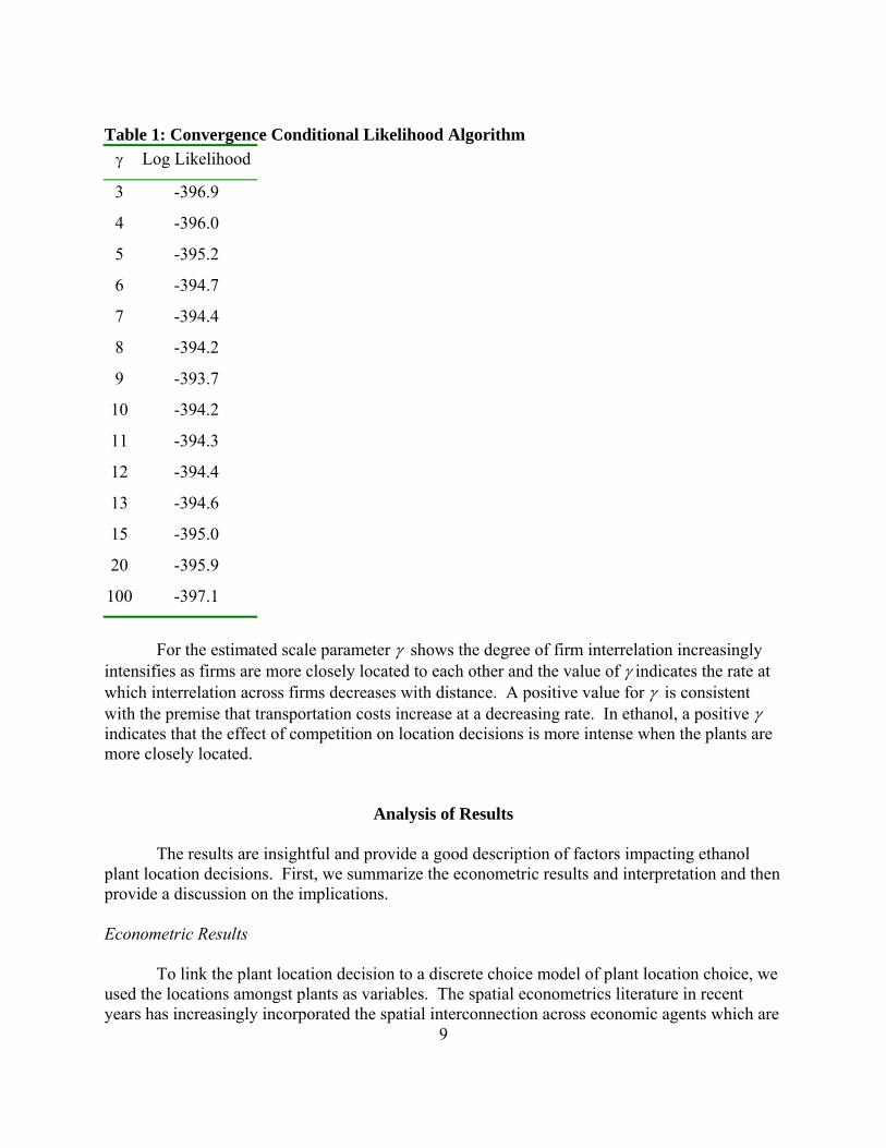
Table 1: Convergence Conditional Likelihood Algorithm γ Log Likelihood

3 -396.9

4 -396.0

5 -395.2

6 -394.7

7 -394.4

8 -394.2

9 -393.7

10 -394.2

11 -394.3

12 -394.4

13 -394.6

15 -395.0

20 -395.9

100 -397.1

For the estimated scale parameter γ shows the degree of firm interrelation increasingly

intensifies as firms are more closely located to each other and the value of γ indicates the rate at which interrelation across firms decreases with distance. A positive value for γ is consistent with the premise that transportation costs increase at a decreasing rate. In ethanol, a positive γ indicates that the effect of competition on location decisions is more intense when the plants are more closely located.

Analysis of Results The results are insightful and provide a good description of factors impacting ethanol plant location decisions. First, we summarize the econometric results and interpretation and then provide a discussion on the implications. Econometric Results To link the plant location decision to a discrete choice model of plant location choice, we used the locations amongst plants as variables. The spatial econometrics literature in recent years has increasingly incorporated the spatial interconnection across economic agents which are

10

important in agricultural industries since these are largely spatial (Anselin 2003; Irwin and Bockstael 2003; Anselin, Bongiovanni, and Lowenberg-DeBoer 2004; Nelson 2002; Nelson and Geoghegan 2002). Existing software used in spatial econometrics, e.g., Spacestat, which has been incorporated into an S-Plus module that works with Arc-View, do not include algorithms for spatial correlation models with a dichotomous dependent variable. Sarmiento and Wilson (2005) developed an algorithm based on concentrating the likelihood function in terms of the spatial correlation coefficient to estimate the model. Factors that determine the probability of plant location in a given county are then analyzed and parameters estimated. Table 1 shows convergence of the algorithm at γ = 9. The algorithm simultaneously estimates parameters of the non-linear logit model with scaling distance factor. Estimation results are shown in Table 2. Several of the agricultural variables are highly significant. Corn yield has a positive but not statistically significant effect on plant location. However, yields of other crops have a negative and statistical effect on ethanol plant location. Of interest are that total planted acres and acres planted to corn have a positive and statistically significant effect on ethanol plant development. Simply, counties with more planted area in total (reflecting in part CRP effects), more area planted to corn, and lower yields of competing crops, have a greater likelihood of ethanol plants locating in that county. Crop production diversification (Herfindahl) index has little explanatory effect on plant location (consistent with Sarmiento and Wilson 2005). Table 2: Ethanol Location Model with Spatial Effects

Coefficient t-value Derivative x Variable

Mean Value Constant Term -4.8128 -14.90 N.A. Corn yield 0.0006 0.43 0.0100 Yields of other crops -0.0019 -1.51 -0.0487 Planted Acreage Corn 0.2599 2.79 0.0338 Planted Acreage Total 0.1037 2.30 0.0400 Herfindahl 0.2625 0.42 0.0025 Total Livestock inventory 0.0000 -0.89 -0.0109 Ethanol subsidy $/gallon 3.9787 3.33 0.0049 Cattle on Feed 0.0004 2.29 0.0112 Hogs on Feed 0.0001 2.65 0.0097 Spatial Competition -22.5969 -2.70 -0.0123 Corn Spatial Lag 0.0001 2.51 0.0075 Log Likelihood -393.7

*Change in the probability from percentage change in the explanatory variable.

The impact of livestock is important. Both cattle and hogs in county j have a positive effect on plant location in that county. We experimented with different measures of feed

11

concentrate demands, but, these results were not significant. These results are largely a reflection of the prospective local demand for feeding of the ethanol byproduct, DDGs. These have difficult shipping and logistical requirements and hence the ability to feed them near the point of ethanol production is important. These results support that observation and why there are concentrations of ethanol production in corn producing regions that have large livestock inventories, as well as dominant feeding regions without corn production (e.g., Texas). The results also show that each of cattle and hogs on feed are important, but the elasticity of the former is greater. This reflects that cattle have a greater ability to consume DDGs than other species.

States compete vigorously to induce ethanol plants to locate within their boundaries. The primary means of competition are state-level subsidies for ethanol production. These values vary across states, are an important source of inter-state competition in these value-added activities and are in addition to the federal subsidy which does not vary across states. These results show that this effect is positive as expected, and its explanatory power is significant. The quantitative effect of the subsidy is illustrated in Figure 1. The result illustrates the nature of competition amongst states in attracting ethanol investment. Simply, assuming all else constant, a greater subsidy increases the probability of a plant being located in a county in that state. Some states (e.g., Minnesota, Nebraska, amongst others) have made extensive use of subsidies to attract plants and these results show that these are effective. However, subsidies alone will not attract investment as having a large supply (production) of corn and livestock inventories to absorb the DDGs is also important.

0.00 0.01 0.02 0.03 0.04 0.05 0.06 0.07 0.08 0.09 0.10

.$0.03 .$0.06 .$0.09 .$0.12 .$0.15 .$0.18 .$0.21 .$0.24 .$0.27 .$0.3

Figure 1. Change in Probability of Plant Location Due to State Subsidy ($ per gallon)

12

The spatial impacts are important and, if not included in the econometric analysis, would result in a misunderstanding of the location decisions. There are two spatial impacts that are important in explaining ethanol location decisions. One is the spatial lag with respect to corn production. Amongst the explanatory variables, only acreage planted to corn has a statistically significant spatial lag effect. That is, statistically, only one spatial lagged explanatory variable is consistent with the data. Results indicate that the spatial externalities in county j (neighboring counties’ corn production) have a positive effect on ethanol plant development on county j. These results are important. An ethanol location decision is impacted not only by corn production in its own county, but it is also impacted by corn production in neighboring counties. This likely is a result of the need to procure corn from more than the county in which the plant is located, but also from neighboring counties, all of which impact the expected payoff in comparing location decisions. The other form of spatial interdependence is the distance to competing plants. This is referred to as spatial competition and it has a negative impact on local plant development. These results show that the effect of competition on plant location is negative and its effect sharply decreases with distance. Figure 2 shows the effects of competition on the probability that a plant locates in a given county. These results show that within about 30 miles the inter-plant spatial competition is important and reduces the likelihood of locating within that range. At 60+ miles apart, the impact on the probability of location in county j is near nil. When controlling for other effects, existence of competition decreases the probability of building a plant in that county, and this impact decreases with distance. This value quantifies the impact of competitor plants in the county and the spatial autocorrelation of competitor plants. The result indicates that existence of competitor plants reduces the likelihood of de-novo ethanol plant locations. This is expected and, no doubt, is reflective of the desire of a new plant to want to avoid competition in procurement with incumbent plants.

-0.0500-0.0450-0.0400-0.0350-0.0300-0.0250-0.0200-0.0150-0.0100-0.00500.0000

20 30 40 50 60 70 80 90 110 130

Miles

Prob

abili

ty

Figure 2. Change in Probability of Plant Location Due to Competition, by Distance.

13

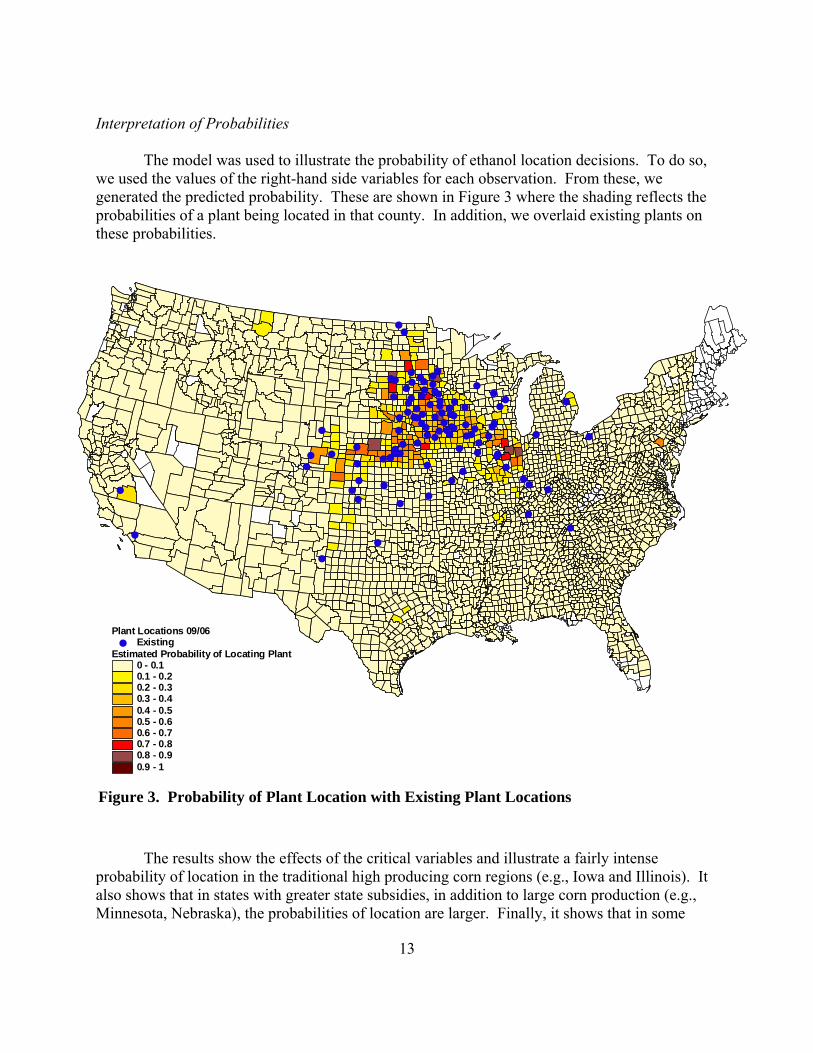
Interpretation of Probabilities The model was used to illustrate the probability of ethanol location decisions. To do so, we used the values of the right-hand side variables for each observation. From these, we generated the predicted probability. These are shown in Figure 3 where the shading reflects the probabilities of a plant being located in that county. In addition, we overlaid existing plants on these probabilities.

The results show the effects of the critical variables and illustrate a fairly intense probability of location in the traditional high producing corn regions (e.g., Iowa and Illinois). It also shows that in states with greater state subsidies, in addition to large corn production (e.g., Minnesota, Nebraska), the probabilities of location are larger. Finally, it shows that in some

#

#

## #

####

## ####

######

# ###

# #

##

#

###

##

#

##

#

##

## #

#

###

###

####

####

###

##

#

##

###

#

######

#

#

#

#

#

###

#

###

#

##

#

#

#

##

#

#

Estimated Probability of Locating Plant0 - 0.10.1 - 0.20.2 - 0.30.3 - 0.40.4 - 0.50.5 - 0.60.6 - 0.70.7 - 0.80.8 - 0.90.9 - 1

Plant Locations 09/06# Existing

Figure 3. Probability of Plant Location with Existing Plant Locations

14

regions with extensive livestock feeding (e.g., Texas, California) there is a higher probability of a plant locating, even though these regions have neither extensive corn production nor state-subsidies.

Summary and Implications

Ethanol is one of the fastest growing industries in the United States agricultural sector. This growth is being driven by numerous factors, but most important are demands for increased ethanol, etc., produced from corn. This has resulted in mammoth investments in value-added agriculture and intense competition among states to attract ethanol location decisions to their states. The purpose of this study was to analyze and determine factors that impact location decisions by new ethanol plants. The model is a discrete logit model of location decisions by new ethanol plants and was specified and estimated using spatial autocorrelation techniques. This allowed an explicit specification to capture spatial impacts on the dependent variable. In addition to the spatial autocorrelation and interdependencies, the model included other agricultural variables, and state level subsidies. The results indicated that location decisions are impacted by the agricultural characteristics of a county, competition, and the state-level subsides. Notably, counties with large areas planted to corn, lower yields of competing crops, and larger cattle inventories, were more likely to attract a new ethanol plant. These decisions are also impacted by spatial competition in two forms. One was the spatial lag of corn production in neighboring counties. This suggests that an ethanol plant location decision is impacted by corn production within the county, as well as in neighboring counties. The second is related to spatial relations amongst competitors. Simply, existence of a competing ethanol plant reduces the likelihood of making a positive location decision and this impact decreases with distance. Finally, state-level subsidies were significant and a very important variable impacting ethanol location decisions. These results have important private and public sector implications. From a private location decision perspective, these results clearly indicate there are a multitude of factors impacting location decisions. Corn supplies are very important, as well as competing crops. In addition, cattle/hog inventories are important as a source of feed demand for the byproduct DDGs. As a result of these, one can expect ethanol locations to be concentrated primarily in counties with large corn production and/or in counties with large cattle/hog inventories. Indeed this is what is being observed with heavy concentration in corn producing states (Iowa, Illinois, Nebraska, and Minnesota) and in counties in Texas, which are heavy feeders. Finally, competing ethanol plants are important and detract from further expansion. This impact is not only local within a county, but has a spatial dimension as well. There are also public sector implications. At least six states have programs to entice ethanol plant locations in the counties in their states. Our results suggest these are significant. Certainly, states such as Minnesota, South Dakota and Nebraska each of which have ethanol

15

subsidies, have enhanced location decisions in their states. However, other factors such as corn production and cattle inventories are important, and in some states are not dominated by the state subsidy. Finally, the logit model with spatial correlation in the choice set used in this study is useful not only in the ethanol sector that was analyzed here, but, could be applied in many other sectors in agricultural industries. For most of these industries, spatial impacts of competition and procurement are important and ignoring them would result in biased estimates and a misunderstanding of factors that impact these decisions. As shown here, the spatial impacts are important to understanding these types of spatial location decisions.

16

References Anselin, L. 2003. “Spatial Externalities.” International Regional Science Review 26:147-152. Anselin, L., R. Bongiovanni, and J. Lowenberg-DeBoer. 2004. “A Spatial Econometric

Approach to the Economics of Site-Specific Nitrogen Management in Corn Production.” American Journal of Agricultural Economics 86:675-687.

Brown, L. 2006. “Ethanol could leave the world hungry,” Fortune, August 16. Business Week. 2006. “Ethanol Fuels ADM’s Performance.” August 12, p56. Collins, K. 2006. Statement of Keith Collins, Chief Economist, U.S. Department of Agriculture

Before the U.S. Senate Committee on Environment and Public Works. September 2, Available at: http://www.usda.gov/oce/newsroom/congressional_testimony/Biofuels%20Tes.

EIA. 2005. Annual Energy Outlook, 2005: With Projections to 2025. U.S. Department of

Energy, Energy Information Administration, Washington, DC, AEO2005. EIA. 2006. Annual Energy Outlook, 2006: With Projections to 2030. U.S. Department of Energy,

Energy Information Administration, Washington, DC, AEO2006. Ethanol Producer Magazine. 2006. “Plant Locations/Planned Expansions.” Accessed 8/7/2006,

Available at: http://www.ethanolproducer.com/plant-list.jsp?country=USA. Fatka, J. 2006a. “CRP not corn’s answer.” Feedstuffs, November 27, p. 1. Fatka, J. 2006b. “Rotations, biotechnology give corn an edge.” Feedstuffs, November 27, p. 1. Feed Management. 1995-2004. “U.S. Feed Market Data.” Feed Management, Sept./Oct. Feltes, R. 2003. Refco Commodity Outlook. Chicago, January. Green, H. 2006. “The Great Corn Rush of 2006: Ethanol profits are drawing in investors, but can

the heydey last?” BusinessWeek, August 14, p. 56. Hart, C. 2006a. “CRP Acreage on the Horizon.” Iowa Ag Review, Spring 2006. Hart, C. 2006b. “Redding the Ethanol Boom: Where wills Corn Come From?” Iowa Ag Review,

Vol. 12(4, Fall):4. Irwin, E.G., and N.E. Bockstael. 2003. “Interacting Agents, Spatial Externalities, and the

Evolution of Residential Land Use Patterns.: Journal of Economic Geography 2:31-54.

17

McMillan, D.P. 1995. “Spatial Effects in Probit Models: A Monte Carlo Investigation.” In New Directions in Spatial Econometrics, Berlin, Heidelberg, New York: Springer-Verlag.

Meyer, P. 2006. “Biotech conference provides venue for discussion of ethanol.” Milling and

Baking News, Sosland Publishing, April 25. National Agricultural Statistics Service. 1995-2005. Agricultural Statistics Database. U.S.

Department of Agriculture, Accessed 8/7/2006, Available at: http://www.nass.usda.gov/index.asp.

Nelson, G.C. 2002. “Introduction to the Special Issue on Spatial Analysis for Agricultural

Economists.” Agricultural Economics 27:197-200.

Nelson, G.C., and J. Geoghegan. 2002. “Deforestation and Land Use Change: Sparse Data Environments.” Agricultural Economics 27:201-16.

Otto, D., and P. Gallagher. 2003. Economic Effects of Current Ethanol Industry Expansion in

Iowa. Iowa State University, June. Available at: Http://www.agmrc.org/NR/rdonlyres/D949FB63-E1D0-40-86CD-5B710B8663DF/0/economiceffectsiaethoanol.pdf.

Pates, M. 2006. “Early Out?: CRP Contract Holders Seek Greener Pastures.” AgWeek, December

11, p. 32. ProExporter. 2004. Grain Transportation Digest. ProExporter, Overland Park, KS, GTB-04-04,

April 8. ProExporter. 2006a. Corn State Supply-Demand and Coastal Exports, The ProExporter Network,

Kansas City, March 10. ProExporter. 2006b. Potential Size and Impact of U.S. Ethanol Expansion. The ProExporter

Network, Kansas City, December 3. ProExporter. 2007. PRX Grain Database, Section 1. Ethanol. The ProExporter Network, Kansas

City, March 7. Red River Farm Network. 2006. Red River Farm Network November 22, Available at: http://www.rrfn.com/. Renewable Fuels Association. Various issues. Plant Locations: U.S. Fuel Ethanol Industry

Plants and Production Capacity. Updated 7/26/2006, Accessed 8/7/2006, Available at: http://www.ethanolrfa.org/industry/locations/.

18

Sarmiento C., and Wilson, W. 2005. Spatial Modeling in Technology Adoption Decisions: The Case of Shuttle Train Elevators. American Journal of Agricultural Economics 87:1033-1044.

Sarmiento C., and Wilson, W. 2007. “Spatially Correlated Exit Strategies.” Applied Economics

39:441-448. Schlicher, M. 2006. Speech to BIO 2006, as reported in Feedstuffs from the National Corn to

Ethanol Research Center. Smith, R. 2006. “Ethanol Production to Create Historic Change.” Feedstuffs, June 5, pp. 24-25. Sosland Publishing. 2006. “Demand surge for ethanol raising questions, but seen as sustainable.”

Milling and Baking News November 7, p.1. Urbanchuk, John M. 2003. The Impact of Growing Ethanol Byproduct Production on Livestock

Feed Markets. Presented at USDA Agricultural Outlook Forum 2003, Arlington, VA, February 20-21.

USDA-ERS. 2003. USDA Outlook Conference, Washington, DC, February. Wulf, G. 2006. “Will Ethanol Finally Bring Gold to Corn Farmers?” The Wall Street Journal,

August. 7, pp C.4.