1

Spatial- and Frequency-Wideband Effects inMillimeter-Wave Massive MIMO Systems

Bolei Wang, Feifei Gao, Shi Jin, Hai Lin, and Geoffrey Ye Li

Abstract—When there are a large number of antennas inmassive MIMO systems, the transmitted wideband signal willbe sensitive to the physical propagation delay of electromagneticwaves across the large array aperture, which is called thespatial-wideband effect. In this scenario, transceiver design isdifferent from most of the existing works, which presume thatthe bandwidth of the transmitted signals is not that wide, ignorethe spatial-wideband effect, and only address the frequencyselectivity. In this paper, we investigate spatial- and frequency-wideband effects, called dual-wideband effects, in massive MIMOsystems from array signal processing point of view. TakingmmWave-band communications as an example, we describe thetransmission process to address the dual-wideband effects. Byexploiting the channel sparsity in the angle domain and the delaydomain, we develop the efficient uplink and downlink channelestimation strategies that require much less amount of trainingoverhead and cause no pilot contamination. Thanks to the arraysignal processing techniques, the proposed channel estimationis suitable for both TDD and FDD massive MIMO systems.Numerical examples demonstrate that the proposed transmissiondesign for massive MIMO systems can effectively deal with thedual-wideband effects.

Index Terms—Massive MIMO, mmWave, array signal process-ing, wideband, spatial-wideband, beam squint, angle reciprocity,delay reciprocity.

I. INTRODUCTION

Massive MIMO, also known as large-scale MIMO, isformed by equipping hundreds or thousands of antennas atthe base station (BS) and can simultaneously serve manyusers in the same time-frequency band. The large number ofantennas in massive MIMO can improve spectrum and energyefficiency, spatial resolution, and network coverage [1]–[3].In the mean time, millimeter-wave (mmWave) communicationmakes massive MIMO more attractive since the small antennasize facilitates packing a large number of antennas in a smallarea at the BS and massive MIMO can combat high path-lossand fading of mmWave channels [3]–[5].

In the past few years, tremendous efforts have been devotedinto the development of massive MIMO as well as its appli-cation in mmWave-band communications. For example, it hasbeen demonstrated in [6]–[8] that large MIMO systems can

B. Wang and F. Gao are with Tsinghua National Laboratory for InformationScience and Technology (TNList), Tsinghua University, Beijing, P. R. China(e-mail: boleiwang@ieee.org, feifeigao@ieee.org).

S. Jin is with the National Communications Research Laboratory, SoutheastUniversity, Nanjing 210096, P. R. China (email: jinshi@seu.edu.cn).

H. Lin is with the Department of Electrical and Information Systems,Graduate School of Engineering, Osaka Prefecture University, Sakai, Osaka,Japan (e-mail: hai.lin@ieee.org).

Geoffrey Ye Li is with the School of Electrical and Computer En-gineering, Georgia Institute of Technology, Atlanta, GA, USA (email:liye@ece.gatech.edu)

enhance spectral efficiency by several orders of magnitude andsimple zero-forcing transceivers are asymptotically optimal.Since channel state information (CSI) is necessary to reach thehuge performance gains for massive MIMO, many differentchannel estimation algorithms [9]–[11] have been designedfor uplink channels while downlink channels can be obtainedby channel reciprocity for time division duplex (TDD) net-works. The calibration error, which may affect the channelreciprocity in the downlink/uplink RF chains, has been alsohandled in [12]. Downlink channel estimation for frequencydivision duplex (FDD) networks has been investigated in [13]–[15]. With a huge number of antennas and the correspondingCSI, beamforming can reach a high spatial resolution [16],[17]. To reduce the cost of hardware implementation, hybridanalog-digital beamforming techniques have been developedfor mmWave-band massive MIMO systems [18]–[22].

Most of the existing works on massive MIMO are based onthe channel model directly extended from the conventionalMIMO channel model [5]–[22]. However, as indicated in[23]–[25], there exists a non-negligible time delay across thearray aperture for the same data symbol in massive MIMOconfiguration. Such phenomenon incurs an inherent propertyof large-size array, called spatial-wideband (spatial-selective)effect. In fact, the spatial-wideband effect has been found inradar systems and has already been well studied in the areaof array signal processing [26], [27]. In the existing massiveMIMO studies, the frequency-selective effect induced by themultipath delay spread has been considered but the spatial-selective effect has been ignored. Therefore, to optimize theperformance, the dual-wideband effects from both the spatialand the frequency domains should be taken into considerationwhen designing massive MIMO systems. If the dual-widebandeffects are considered, many fundamental issues for massiveMIMO, which have been obtained by using the extended con-ventional MIMO channel models, will need to be reformulatedand the previous results will be revised.

In this paper, we investigate the massive MIMO commu-nications by considering the dual-wideband effects from thearray signal processing viewpoint. By exploiting the channelsparsity in both angle and delay domains, a massive MIMOchannel with the dual-wideband effects is modeled as a func-tion of limited parameters, e.g., the complex gain, the directionof arrival (DOA) or the direction of departure (DOD), and thetime delay of each channel path. We then develop channelestimation techniques for both the uplink and downlink casesin massive MIMO systems, which require significantly lessamount of training overhead and have no pilot contamination.Furthermore, we will reveal that the angle and the delay

arX

iv:1

708.

0760

5v5

[cs

.IT

] 2

6 A

pr 2

018

2

domains, or the spatial and the frequency domains, exhibitstrong duality in various aspects, which can help the trainingdesign as well as the subsequent data transmission. Moreover,the proposed channel estimation strategy is suitable for bothTDD and FDD massive MIMO systems due to the angleand the time delay reciprocities. Computer simulation resultsdemonstrate that the proposed channel estimation strategiesfor massive MIMO systems can effectively deal with the dual-wideband effects while the existing designs cannot.

The rest of this paper is organized as follows. Section IIintroduces the array signal processing theory as well as therationale of the spatial-wideband effect. Section III formulatesthe new channel model of massive MIMO systems consideringthe dual-wideband effects. Section IV addresses the massiveMIMO channel estimation with the dual-wideband effects.Numerical results are provided in Section V, and Section VIconcludes this paper.Notations:

(·)T transpose of a matrix or a vector(·)H conjugate transpose or Hermitian operation

of a matrix or a vector(·)∗ conjugate of a matrix or a vector(·)† pseudo-inversion of a matrix or a vector

I identity matrix1 all-ones matrix0 all-zeros matrix◦ Hadamard product of two matrices⊗ Kronecker product of two matrices

E{·} expectation operationtr(·) matrix trace operation‖a‖2 Euclidean norm of vector a

diag{a} the diagonal matrix comprising vector a’selements

‖A‖F Frobenius norm of matrix A[A]m,n the (m,n)th element of the matrix A[A]:,n the nth column of the matrix A[A]m,: the mth row of the matrix A

diag{A} the vector extracted from diagonal entries ofmatrix A

|A| cardinality of set AI(M) set I(M) � {0, 1, . . . ,M − 1}�{·} real part of a complex number, vector or matrix

II. SPATIAL-WIDEBAND EFFECT OF LARGE-SCALE ARRAY

In this section, we present the principle of the spatial-wideband effect in large-scale arrays and discuss why it canbe ignored in small-scale MIMO systems.

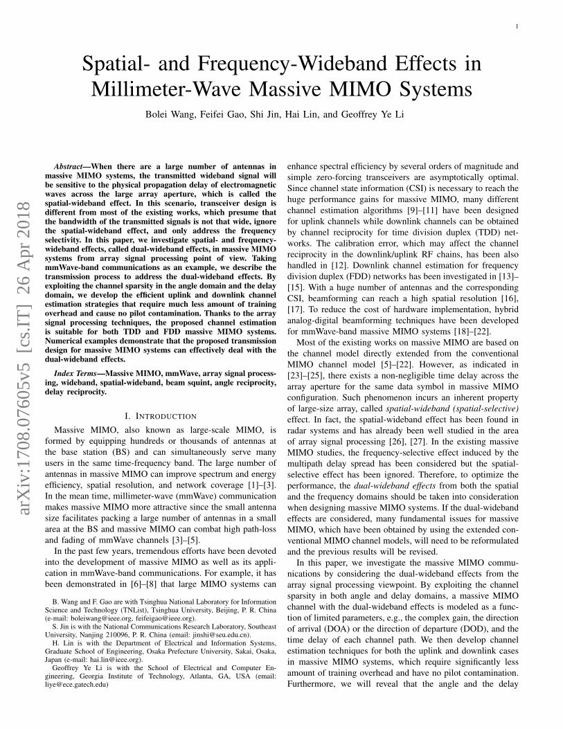
As in Fig. 1, consider a signal from far-field source im-pinging onto a uniform linear array (ULA) 1 of M antennaswith a single direction ϑ. Let the antenna spacing be d, thecarrier wavelength be λc, and the carrier frequency be fc.Denote ψ � d sinϑ

λcfor notation simplicity. Then, the time

1In this paper, we employ the ULA to clearly illustrate the nature ofthe spatial-wideband effect and the corresponding channel characteristics.Nevertheless, the spatial-wideband effect exists in all large-scale antennasregardless of array topology as long as the propagation delay across the arrayaperture is non-ignorable compared with the symbol duration.

Fig. 1. An illustration of the spatial-wideband effect of a ULA with Mantennas.

delay between adjacent antennas can be explicitly computedas d sinϑ

c = ψfc

, where c is the speed of light.For a communication system with single-carrier modulation

of the symbol period, Ts, the baseband signal can be repre-sented as

s(t) =

+∞∑

i=−∞s[i]g(t− iTs), (1)

where g(t) is the pulse shaping function and s[i] is thetransmit symbols. The corresponding passband signal canbe represented as �{s(t)ej2πfct} and the bandwidth of themodulated signal is around 1

Ts.

Without loss of generality, assume that the first anten-na is perfectly synchronized with the source and receives�{αs(t)ej2πfct}, where α is the complex channel gain.Then, the other antennas will receive a delayed version of�{αs(t)ej2πfct}.

From Fig. 1, the time interval between the 0th and the mthantenna is m ψ

fc, and the passband signal received by the mth

antenna can be expressed as

�{αs

(t−m

ψ

fc

)ej2πfc(t−m ψ

fc)

}

= �{αs

(t−m

ψ

fc

)e−j2πmψej2πfct

}. (2)

Therefore, the equivalent baseband signal received by the mthantenna is

ym(t) � αs

(t−m

ψ

fc

)e−j2πmψ. (3)

A. Small Array or Spatial-Narrowband Effect

If the number of antenna M is small, or the transmissionbandwidth of s(t) is narrow, then m ψ

fc� Ts and s(t−m ψ

fc) ≈

s(t) hold for ∀m ∈ I(M). In this case, the received signalvector from all M antennas can be represented by

y(t) = [y0(t), y1(t), . . . , yM−1(t)]T

= αs(t)[1, e−j2πψ, . . . , e−j2π(M−1)ψ]T � αs(t)a(ψ),(4)

3

where a(ψ) is known as the spatial steering vector pointingtowards the angle ϑ. The equivalent baseband channel vectorwill be h = αa(ψ). As a result, the baseband channel can berepresented as [11], [29]

h =

L−1∑

l=0

αla(ψl)δ(t− τl), (5)

where L is the number of channel paths,2 ψl � d sinϑl

λc, ϑl

denotes the DOA of the lth path, τl is the corresponding pathdelay, and δ(·) is the Dirac impulse function.

It should be emphasized that the assumption m ψfc

� Ts,which requires the symbol duration Ts to be large enoughor the baseband signal s(t) to be relatively narrowband, is anecessary condition for making the small-scale MIMO channelmodel (5) and other derived models hold.

B. Large Array and Spatial-Wideband Effect

For wideband massive MIMO system, M is usually verylarge, and the transmit baseband signal s(t) has wide band-width. In this case, the approximation, s(t − m ψ

fc) ≈ s(t),

does not hold for the larger indices m any more, making (4)and (5) invalid.

For example, for a ULA system equipped with M = 128antennas and the antenna spacing d = λc/2, when the incidentpath comes from ϑ = 60◦, the propagation delay across thearray aperture is 0.58Ts in a typical LTE system with thetransmission bandwidth fs = 20 MHz at fc = 1.9 GHz. Asfor the typical mmWave-band system with fs = 1 GHz atfc = 60 GHz, such delay will be 0.92Ts.

More specifically, if m ψfc

is comparable to Ts or even largerthan Ts, then the mth antenna would “see” a different transmitsymbol from the 0th antenna. This phenomenon is called thespatial-wideband effect in array signal processing, which hasbeen well studied in radar signal processing but is seldomdiscussed in wireless communications where the number ofantennas is not large enough or the signal bandwidth is notthat wide.

In massive MIMO systems, especially over mmWave-band,the narrowband assumption does not hold any more. In thiscase, the conventional massive MIMO channel model (5) andother models that directly extended from the conventionalmodels, will be inapplicable. As will be seen in the lat-er numerical results, the algorithms without considering thespatial-wideband effect will suffer from the performance losswhen either the number of BS antennas or the transmissionbandwidth becomes large. It has been discovered in [30] thatthe performance of the phased-array hybrid structure willdegrade due to the spatial-wideband effect as the bandwidthincreases.

2When there are rich scatters around the BS, especially in low frequencyband, many paths would arrive at an approximately identical time delay andformulate one channel tap. In this case, each summand in (5) would be coupledby an integration over the incoming angular spread corresponding to eachspecific channel tap.

III. MASSIVE MIMO CHANNELS WITH DUAL-WIDEBANDEFFECTS

As discussed previously, the spatial-wideband effect, as aninherent property of large-scale arrays, must be considered ina real massive MIMO systems. In this section, we will firstmodel the massive MIMO channels with the dual-widebandeffects and then discuss its impact on the orthogonal frequencydivision multiplexing (OFDM) transmission scheme. More-over, several fundamental characteristics of the dual-widebandchannel are also investigated to aid the channel estimation andthe user scheduling designs in the next section.

A. Channel Modeling with Dual-Wideband Effects

Let us consider a massive MIMO system consisting of oneBS with an M -antenna ULA and P randomly distributedusers, each with a single antenna. We will address the dual-wideband effects in OFDM scheme since it is used in mostbroadband wireless communications protocols. The number ofOFDM subcarriers is denoted as N . For ease of illustration,we consider the mmWave-band transmission and suppose thatthere are Lp individual physical paths between the BS and thepth user.3

Denote τp,l,m as the time delay of the lth path from the pthuser to the mth antenna, which is not necessarily an integermultiple of Ts. Then the received baseband signal at the mthantenna from the pth user can be expressed as

yp,m(t) =

Lp−1∑

l=0

αp,lxp(t− τp,l,m)e−j2πfcτp,l,m , (6)

where αp,l is the corresponding complex channel gain, andxp(t) is the transmitted signal of the pth user. Denote the DOAof the lth path of user p as ϑp,l, and define ψp,l � d sinϑp,l

λc.

From Fig. 1, we have

τp,l,m = τp,l,0 +mψp,l

fc, m ∈ I(M). (7)

For notation simplicity, we denote τp,l � τp,l,0 in the rest ofthis paper.

With (7), equation (6) can be rewritten as

yp,m(t) =

Lp−1∑

l=0

αp,le−j2πfcτp,lxp

(t− τp,l −m

ψp,l

fc

)e−j2πfcm

ψp,lfc

=

Lp−1∑

l=0

αp,lxp

(t− τp,l −m

ψp,l

fc

)e−j2πmψp,l , (8)

where αp,l � αp,le−j2πfcτp,l is the equivalent channel gain.

3The extension to low frequency-band communications can be straightfor-wardly made by counting the angular spread caused by local scattering [15],[31].

4

Then, the uplink spatial-time channel of the pth user at themth antenna can be modeled as

[hST,p(t)]m =

Lp−1∑

l=0

αp,l[a(ψp,l)]mδ(t− τp,l,m)

=

Lp−1∑

l=0

αp,l[a(ψp,l)]mδ

(t− τp,l −m

ψp,l

fc

).

(9)

Taking the continuous time Fourier transform (CTFT) of(9), we obtain the uplink spatial-frequency response of thepth user at the mth antenna as

[hSF,p(f)]m =

∫ +∞

−∞[hST,p(t)]me−j2πftdt

=

Lp−1∑

l=0

αp,l[a(ψp,l)]me−j2πfτp,l,m

=

Lp−1∑

l=0

αp,le−j2πmψp,le−j2πfτp,le−j2πfm

ψp,lfc .

(10)

Denote the subcarrier spacing of OFDM as η = fsN Hz. Then,

the spatial-frequency channel coefficients of the nth subcarriercan be expressed as [hSF,p(nη)]m, ∀n ∈ I(N). The overallspatial-frequency channel matrix from all M antennas can thenbe formulated as

Hp = [hSF,p(0),hSF,p(η), . . . ,hSF,p((N − 1)η)]

=

Lp−1∑

l=0

αp,l

(a(ψp,l)b

T (τp,l))◦Θ(ψp,l), (11)

where “◦” denotes the Hadamard product and

b(τp,l) � [1, e−j2πητp,l , . . . , e−j2π(N−1)ητp,l ]T ∈ CN×1

(12)

can be viewed as “frequency-domain steering vector” pointingtowards the lth delay of the pth user. Moreover, Θ(ψp,l) is anM ×N matrix whose (m,n)th element is

[Θ(ψp,l)]m,n � exp

(−j2πmnη

ψp,l

fc

),

m ∈ I(M), n ∈ I(N). (13)

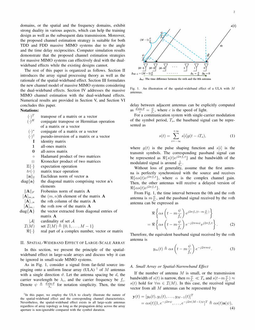
Clearly, the equations (11)-(13) provide a more accuratechannel model for large-scale antennas by considering boththe spatial- and frequency- wideband effects (dual-widebandeffects). In this case, the spatial steering vector a(ψp,l) iscoupled with the frequency-domain steering vector b(τp,l), aswell as the phase shift matrix Θ(ψp,l). We then call (11) thespatial-frequency wideband (SFW) channel (dual-widebandchannel). It should be noted that the beam squint effect, whichinduces the frequency-dependent radiation pattern of a large-scale array [32], is fully considered in the proposed model(11) and expressed by the phase shift matrix Θ(ψp,l).

Compared with the conventional small-scale MIMO channelmodel (5), the phase shift matrix Θ(ψp,l) for each path arisesdue to the spatial-wideband effect. The maximum phase shift

2D-IDFT 2D-DFTIDFT DFT IDFT DFT

Spatial Frequency

Angle Delay

Spatial-frequencyChannel

Angular-delayChannel

Fig. 2. Duality between the angle domain and the delay domain, as well asbetween their Fourier transform: spatial domain and frequency domain.

BCP[1] B[1]B[0]

BCP[1] B[1]B[0]

BCP[2]

BCP[2]

BCP[1] B[1]B[0]

BCP[1] B[1]B[0]BCP[0]

B[1

B[1]

BCP[1] B[

BCP[1] B

111111]]]]]]

B[1[[[[[[

The actual received signal that contains

an intact OFDM symbol

]

BB

T

Examples of synchronization point

Minimum CP length

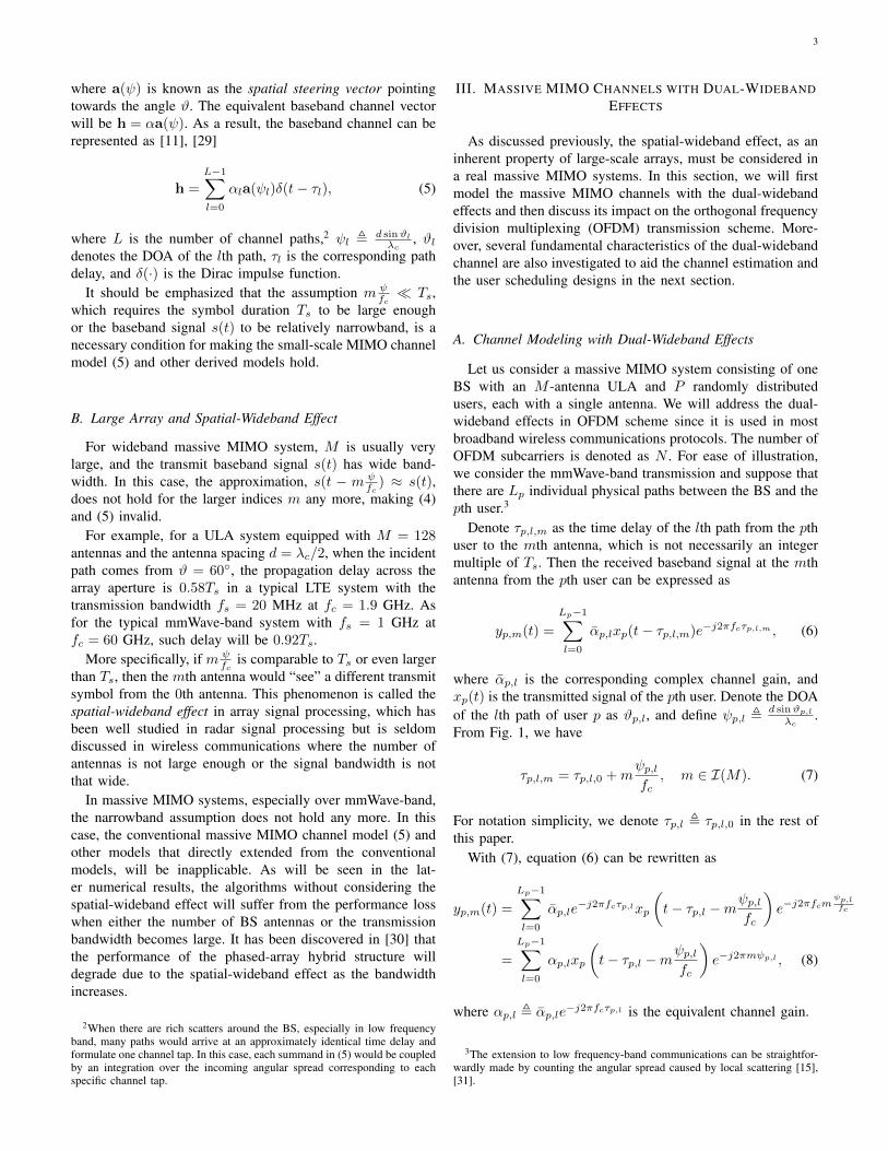
Fig. 3. An illustration of the effect of a single path in SFW channels, whereB[i] denotes the ith OFDM symbol.

inside this matrix can be approximately fsfc

dλcM . In small-

scale antennas with small M or in large-scale antennas butwith very narrow bandwidth fs, the maximum phase shift isfsfc

dλcM � 1 and close to zero such that the phase shift matrix

Θ(ψp,l) for each path is an approximate all-ones matrix inconformity to the analysis in Sec. II.

Interestingly, “angle” domain and “delay” domain are cou-pled in a dual manner in (11). Similar duality also appearsin their Fourier transforms: “spatial” domain and “frequency”domain, as illustrated in Fig. 2. For example, the angularbeamforming and the temporal beamforming can be realizedby weighting the antennas in spatial domain and the subcarri-ers in the frequency domain, in a similar way. Moreover, theenergy of each path in angular-delay domain is diffused forthe same level in the angle and the delay dimensions, as willbe seen in Theorem 1 in Sec. III-C.

B. Essential Requirement of CP Length for OFDM

The SFW channel model (11) implicitly requires that thecyclic prefix (CP) of OFDM modulation is sufficiently long toovercome the channel delay at each individual antenna.

To better illustrate how to choose CP length, we firstdemonstrate the lth path of user p in Fig. 3, where B[i]denotes the ith time-domain OFDM block of the pth user,and BCP [i] represents the corresponding CP. Take B[1] for

5

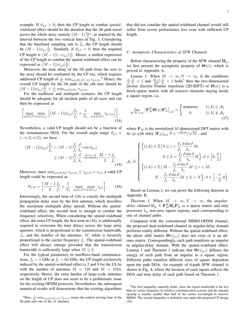
example. If ϑp,l > 0, then the CP length to combat spatial-wideband effect should be the duration that the lth path travelacross the whole array, namely (M−1)

ψp,l

fc, as marked by the

interval between the two vertical lines in Fig. 3. Consideringthat the baseband sampling rate is fs, the CP length shouldbe (M − 1)ψp,l

fsfc

. Similarly, if ϑp,l < 0, then the requiredCP length is (M − 1)(−ψp,l)

fsfc

. Hence, a unified expressionof the CP length to combat the spatial-wideband effect can beexpressed as (M − 1)|ψp,l| fsfc .

Moreover, the time delay of the lth path from the user tothe array should be combatted by the CP too, which requiresadditional CP length of 1

Tsminm∈{0,M−1} τp,l,m.4 Hence, the

overall CP length for the lth path of the pth user should be(M − 1)|ψp,l| fsfc + 1

Tsminm∈I(M) τp,l,m.

For the multiuser and multipath scenario, the CP lengthshould be adequate for all incident paths of all users and canthen be expressed as⌈max

p∈I(P )max

l∈I(Lp)

[(M − 1)|ψp,l|

fsfc

+1

Ts· minm∈I(M)

τp,l,m

]⌉.

(14)

Nevertheless, a valid CP length should not be a function ofthe instantaneous DOA. For the overall angle range ϑp,l ∈(−π/2, π/2), we have

(M − 1)|ψp,l|fsfc

= (M − 1)fsfc

d

λc| sinϑp,l|

≤ (M − 1)fsfc

d

λc

d=λc/2======

M − 1

2

fsfc

.

(15)

Moreover, since minm∈I(M) τp,l,m ≤ τp,l,0 = τp,l, a valid CPlength could be expressed as

NCP =

⌈M − 1

2

fsfc

+1

Ts· maxp∈I(P )

maxl∈I(Lp)

τp,l

⌉. (16)

Interestingly, the second item of (16) is exactly the multipathpropagation delay seen by the first antenna, which describesthe maximum multipath delay spread. Without the spatial-wideband effect, the second item is enough to combat thefrequency selectivity. When considering the spatial-widebandeffect, the extra CP length, the first term in (16), is additionallyrequired to overcome the time delays across the large arrayaperture, which is proportional to the transmission bandwidth,fs, and the number of the antennas, M , while is inverselyproportional to the carrier frequency fc. The spatial-widebandeffect will always emerge provided that the transmissionbandwidth is sufficiently large when M ≥ 2.

For the typical parameters in mmWave-band communica-tions, fs = 1 GHz at fc = 60 GHz, the CP length exclusivelyinduced by the spatial-wideband effect is 2 and 9 for the ULAswith the number of antennas M = 128 and M = 1024,respectively. Hence, the extra burden of large-scale antennason the length of CP does not seem to be a problematic issuefor the existing OFDM protocols. Nevertheless, the subsequentnumerical results will demonstrate that the existing algorithms

4Here, 1Ts

minm∈{0,M−1} τp,l,m means the earliest arriving time of thelth path onto one of the M antennas.

that did not consider the spatial-wideband channel would stillsuffer from severe performance loss even with sufficient CPlength.

C. Asymptotic Characteristics of SFW Channels

Before characterizing the property of the SFW channel Hp,we first present the asymptotic property of Θ(ψ), which isproved in Appendix A.

Lemma 1: When M → ∞, N → ∞, if the conditionsfsfc

dλc

< 1 and M−12N

fsfc

< 1 hold,5 then the two-dimensionalinverse discrete Fourier transform (2D-IDFT) of Θ(ψ) is ablock-sparse matrix with all nonzero elements staying insidea square region, i.e.,

limM,N→∞

[FH

MΘ(ψ)F∗N

]i,k

=

{nonzeros (i, k) ∈ A1

0 (i, k) /∈ A1

(17)

where FM is the normalized M -dimensional DFT matrix withits (p, q)th entry [FM ]p,q � e−j 2π

M pq/√M , and

A1 �

⎧⎪⎪⎪⎪⎪⎪⎪⎪⎪⎪⎨⎪⎪⎪⎪⎪⎪⎪⎪⎪⎪⎩

{(i, k) ∈ Z

∣∣ 0 ≤ i <fsfc

d sinϑ

λcM,

0 ≤ k <fsfc

d sinϑ

λcM}, ϑ ∈

[0,

π

2

]

{(i, k) ∈ Z

∣∣M − fsfc

d sinϑ

λcM ≤ i < M,

N − fsfc

d sinϑ

λcM ≤ k < N

}, ϑ ∈

[−π

2, 0)

.

Based on Lemma 1, we can prove the following theorem inAppendix B.

Theorem 1: When M → ∞, N → ∞, the angular-delay channel Gp � FH

MHpF∗N is a sparse matrix and only

possesses Lp non-zero square regions, each corresponding toone of channel paths.

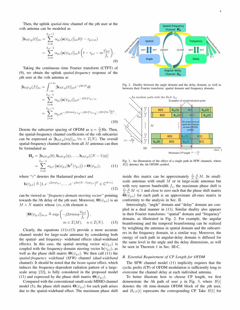
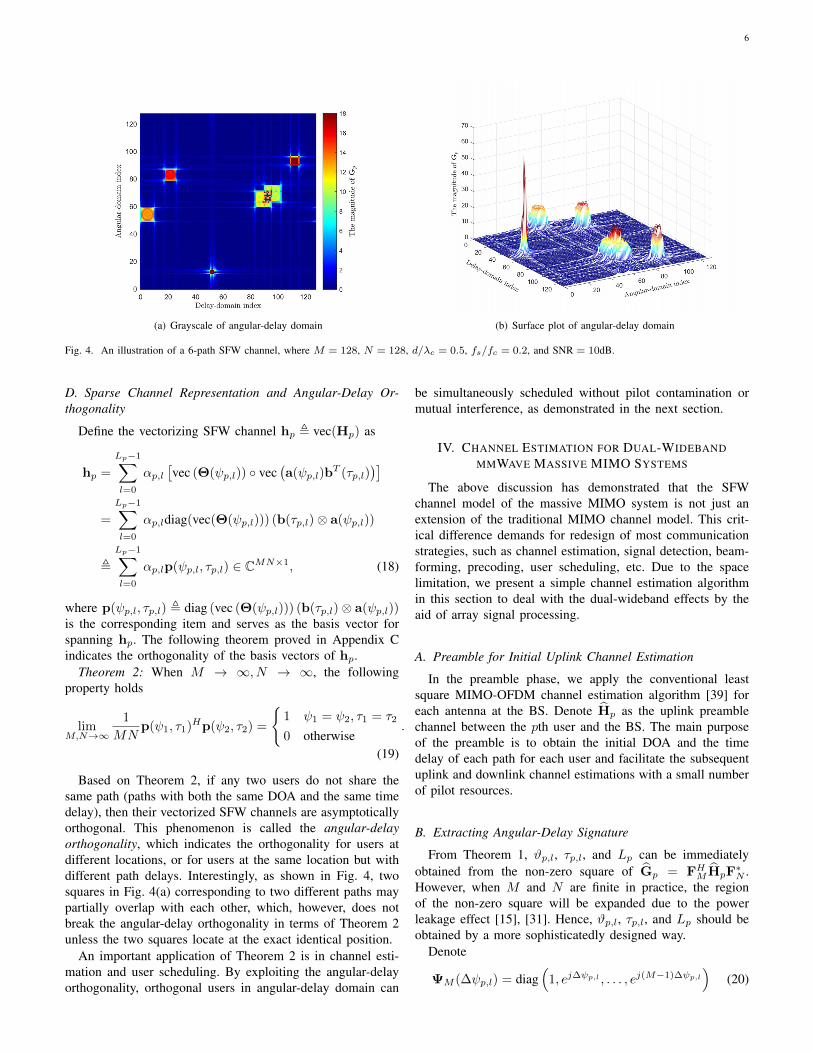
Compared with the conventional MIMO-OFDM channel,the proposed dual-wideband channel in angular-delay domainperforms totally different. Without the spatial-wideband effect,the phase shift matrix Θ(ψp,l) does not exist or is an all-ones matrix. Correspondingly, each path manifests an impulsein angular-delay domain. With the spatial-wideband effect,Lemma 1 and Theorem 1 indicate that Θ(ψp,l) diffuses theenergy of each path from an impulse to a square region.Different paths manifest different sizes of square dependentupon the path DOA. An example of 6-path SFW channel isshown in Fig. 4, where the location of each square reflects theDOA and time delay of each path based on Theorem 1.

5The first inequality naturally holds, since the signal bandwidth is far lessthan its carrier frequency in wireless communication systems and the antennaspacing is usually smaller than half of the carrier wavelength in massiveMIMO. The second inequality is definitely true under the proposed CP design(16).

6

(a) Grayscale of angular-delay domain (b) Surface plot of angular-delay domain

Fig. 4. An illustration of a 6-path SFW channel, where M = 128, N = 128, d/λc = 0.5, fs/fc = 0.2, and SNR = 10dB.

D. Sparse Channel Representation and Angular-Delay Or-thogonality

Define the vectorizing SFW channel hp � vec(Hp) as

hp =

Lp−1∑

l=0

αp,l

[vec (Θ(ψp,l)) ◦ vec

(a(ψp,l)b

T (τp,l))]

=

Lp−1∑

l=0

αp,ldiag(vec(Θ(ψp,l))) (b(τp,l)⊗ a(ψp,l))

�Lp−1∑

l=0

αp,lp(ψp,l, τp,l) ∈ CMN×1, (18)

where p(ψp,l, τp,l) � diag (vec (Θ(ψp,l))) (b(τp,l)⊗ a(ψp,l))is the corresponding item and serves as the basis vector forspanning hp. The following theorem proved in Appendix Cindicates the orthogonality of the basis vectors of hp.

Theorem 2: When M → ∞, N → ∞, the followingproperty holds

limM,N→∞

1

MNp(ψ1, τ1)

Hp(ψ2, τ2) =

{1 ψ1 = ψ2, τ1 = τ2

0 otherwise.

(19)

Based on Theorem 2, if any two users do not share thesame path (paths with both the same DOA and the same timedelay), then their vectorized SFW channels are asymptoticallyorthogonal. This phenomenon is called the angular-delayorthogonality, which indicates the orthogonality for users atdifferent locations, or for users at the same location but withdifferent path delays. Interestingly, as shown in Fig. 4, twosquares in Fig. 4(a) corresponding to two different paths maypartially overlap with each other, which, however, does notbreak the angular-delay orthogonality in terms of Theorem 2unless the two squares locate at the exact identical position.

An important application of Theorem 2 is in channel esti-mation and user scheduling. By exploiting the angular-delayorthogonality, orthogonal users in angular-delay domain can

be simultaneously scheduled without pilot contamination ormutual interference, as demonstrated in the next section.

IV. CHANNEL ESTIMATION FOR DUAL-WIDEBANDMMWAVE MASSIVE MIMO SYSTEMS

The above discussion has demonstrated that the SFWchannel model of the massive MIMO system is not just anextension of the traditional MIMO channel model. This crit-ical difference demands for redesign of most communicationstrategies, such as channel estimation, signal detection, beam-forming, precoding, user scheduling, etc. Due to the spacelimitation, we present a simple channel estimation algorithmin this section to deal with the dual-wideband effects by theaid of array signal processing.

A. Preamble for Initial Uplink Channel Estimation

In the preamble phase, we apply the conventional leastsquare MIMO-OFDM channel estimation algorithm [39] foreach antenna at the BS. Denote Hp as the uplink preamblechannel between the pth user and the BS. The main purposeof the preamble is to obtain the initial DOA and the timedelay of each path for each user and facilitate the subsequentuplink and downlink channel estimations with a small numberof pilot resources.

B. Extracting Angular-Delay Signature

From Theorem 1, ϑp,l, τp,l, and Lp can be immediatelyobtained from the non-zero square of Gp = FH

MHpF∗N .

However, when M and N are finite in practice, the regionof the non-zero square will be expanded due to the powerleakage effect [15], [31]. Hence, ϑp,l, τp,l, and Lp should beobtained by a more sophisticatedly designed way.

Denote

ΨM (Δψp,l) = diag(1, ejΔψp,l , . . . , ej(M−1)Δψp,l

)(20)

7

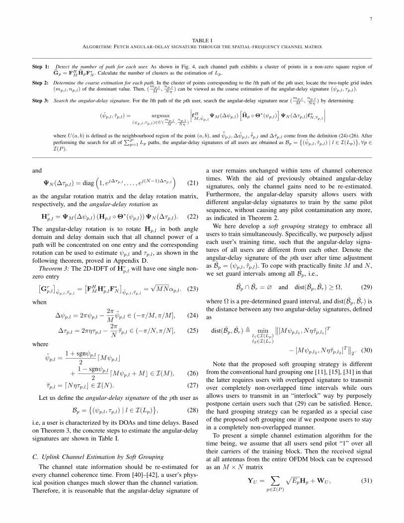
TABLE IALGORITHM: FETCH ANGULAR-DELAY SIGNATURE THROUGH THE SPATIAL-FREQUENCY CHANNEL MATRIX

Step 1: Detect the number of path for each user. As shown in Fig. 4, each channel path exhibits a cluster of points in a non-zero square region ofGp = FH

M HpF∗N . Calculate the number of clusters as the estimation of Lp.

Step 2: Determine the coarse estimation for each path. In the cluster of points corresponding to the lth path of the pth user, locate the two-tuple grid index(mp,l, np,l) of the dominant value. Then, (

mp,l

M,np,l

Nη) can be viewed as the coarse estimation of the angular-delay signature (ψp,l, τp,l).

Step 3: Search the angular-delay signature. For the lth path of the pth user, search the angular-delay signature near (mp,l

M,np,l

Nη) by determining

(ψp,l, τp,l) = argmax(ψp,l,τp,l)∈U(

mp,lM

,np,lNη

)

∣∣∣∣fHM,ψp,lΨM (Δψp,l)

[Hp ◦Θ∗(ψp,l)

]ΨN (Δτp,l)f

∗N,τp,l

∣∣∣∣

where U(a, b) is defined as the neighbourhood region of the point (a, b), and ˆψp,l,Δψp,l, ˆτp,l and Δτp,l come from the definition (24)-(26). After

performing the search for all of∑P

p=1 Lp paths, the angular-delay signatures of all users are obtained as Bp ={(ψp,l, τp,l) | l ∈ I(Lp)

}, ∀p ∈

I(P ).

and

ΨN (Δτp,l) = diag(1, ejΔτp,l , . . . , ej(N−1)Δτp,l

)(21)

as the angular rotation matrix and the delay rotation matrix,respectively, and the angular-delay rotation as

Hrp,l = ΨM (Δψp,l) (Hp,l ◦Θ∗(ψp,l))ΨN (Δτp,l). (22)

The angular-delay rotation is to rotate Hp,l in both angledomain and delay domain such that all channel power of apath will be concentrated on one entry and the correspondingrotation can be used to estimate ψp,l and τp,l, as shown in thefollowing theorem, proved in Appendix D.

Theorem 3: The 2D-IDFT of Hrp,l will have one single non-

zero entry[Gr

p,l

]ψp,l,τp,l

=[FH

MHrp,lF

∗N

]ψp,l,τp,l

=√MNαp,l. (23)

when

Δψp,l = 2πψp,l −2π

Mψp,l ∈ (−π/M, π/M ], (24)

Δτp,l = 2πητp,l −2π

Nτp,l ∈ (−π/N, π/N ], (25)

where

ψp,l =1 + sgnψp,l

2�Mψp,l�

+1− sgnψp,l

2�Mψp,l +M� ∈ I(M), (26)

τp,l = �Nητp,l� ∈ I(N). (27)

Let us define the angular-delay signature of the pth user as

Bp ={(ψp,l, τp,l) | l ∈ I(Lp)

}, (28)

i.e, a user is characterized by its DOAs and time delays. Basedon Theorem 3, the concrete steps to estimate the angular-delaysignatures are shown in Table I.

C. Uplink Channel Estimation by Soft Grouping

The channel state information should be re-estimated forevery channel coherence time. From [40]–[42], a user’s phys-ical position changes much slower than the channel variation.Therefore, it is reasonable that the angular-delay signature of

a user remains unchanged within tens of channel coherencetimes. With the aid of previously obtained angular-delaysignatures, only the channel gains need to be re-estimated.Furthermore, the angular-delay sparsity allows users withdifferent angular-delay signatures to train by the same pilotsequence, without causing any pilot contamination any more,as indicated in Theorem 2.

We here develop a soft grouping strategy to embrace allusers to train simultaneously. Specifically, we purposely adjusteach user’s training time, such that the angular-delay signa-tures of all users are different from each other. Denote theangular-delay signature of the pth user after time adjustmentas Bp = (ψp,l, τp,l). To cope with practically finite M and N ,we set guard intervals among all Bp, i.e.,

Bp ∩ Br = ∅ and dist(Bp, Br) ≥ Ω, (29)

where Ω is a pre-determined guard interval, and dist(Bp, Br) isthe distance between any two angular-delay signatures, definedas

dist(Bp, Br) � minl1∈I(Lp)l2∈I(Lr)

∥∥[Mψp,l1 , Nητp,l1 ]T

− [Mψp,l2 , Nητp,l2 ]T∥∥2. (30)

Note that the proposed soft grouping strategy is differentfrom the conventional hard grouping one [11], [15], [31] in thatthe latter requires users with overlapped signature to transmitover completely non-overlapped time intervals while oursallows users to transmit in an “interlock” way by purposelypostpone certain users such that (29) can be satisfied. Hence,the hard grouping strategy can be regarded as a special caseof the proposed soft grouping one if we postpone users to stayin a completely non-overlapped manner.

To present a simple channel estimation algorithm for thetime being, we assume that all users send pilot “1” over alltheir carriers of the training block. Then the received signalat all antennas from the entire OFDM block can be expressedas an M ×N matrix

YU =∑

p∈I(P )

√EpHp +WU , (31)

8

where√Ep is the training power constraint for user p, and

WU ∈ CM×N is the independent additive white Gaussiannoise matrix with each element distributed as CN (0, σ2

n).By exploiting the angular-delay orthogonality of SFW chan-

nels and the obtained signatures of all users, the complexchannel gain of each path can be simply updated as6

αp,l ≈1

MN√

Ep

p(ψp,l, τp,l)Hvec(YU ). (32)

The uplink channel of the pth user can then be reconstructedby the updated complex gain with the corresponding angular-delay signatures as

HUp =

∑

l∈I(Lp)

αp,l

(a(ψp,l)b

T (τp,l))◦Θ(ψp,l), (33)

where ψp,l and τp,l are obtained during the preamble and thesoft-grouping process.

From (11) or (18), the high-dimensional SFW channelcan be represented in a sparse form determined by the 3Lp

parameters, ϑp,l (or the equivalent ψp,l), τp,l, and αp,l.

D. Downlink Channel Representation

It has been shown in [43], [44] that the physical DOAs ϑp,l

and path delays τp,l are roughly the same for the uplink anddownlink transmission even in FDD systems7, which is calledthe angular-delay reciprocity. Denote the downlink carrierfrequency as fD

c and the corresponding carrier wavelength asλDc . According to the angular-delay reciprocity, ψp,l in the

downlink channel can be directly obtained from

ψDp,l =

d sinϑp,l

λDc

=d sinϑp,l

λc

fDc

fc=

fDc

fcψp,l. (34)

Similar to the uplink case, we can use the soft groupingmethod by adjusting the path delay from τp,l to τDp,l andthen obtain the downlink signature BD

p . The adjustment obeysthe same rule as (29) expect for replacing (ψp,l, τp,l) by(ψD

p,l, τDp,l).

Denote the downlink channel from the BS towards the pthuser as

(HD

p

)H ∈ CN×M . Similar to (11), the downlinkspatial-frequency channel can be modeled as

HDp =

Lp−1∑

l=0

βp,l

(a(ψD

p,l)bT (τDp,l)

)◦Θ(ψD

p,l) ∈ CM×N .

(35)

As a result, we only need to estimate the corresponding βp,l

in (35) to obtain the downlink channel.

6As long as the angular-delay signatures of users change slowly, one canalso obtain the updated angular-delay signatures from (31) with Algorithm1, where the non-zero blocks of all users can be distinguished thanks to theproposed soft grouping method.

7This characteristic of electromagnetic wave holds when the intervalbetween the downlink and the uplink frequency is within several gigahertz(GHz).

E. Downlink Channel Estimation

Let us assume that the users contain the same number ofpaths LM and the training is performed over LM blocks.Denote hD

p � vec(HDp ) ∈ CMN×1. The downlink channel

between the BS and the pth user can be expressed as

(hDp )H =

Lp−1∑

l=0

(βp,l)∗pH(ψD

p,l, τDp,l) = βH

p PHp , (36)

where βp = [βp,0, βp,1, . . . , βp,Lp−1]T is the downlink chan-

nel gain vector and Pp ∈ CMN×LM is defined as

Pp �[p(ψD

p,0, τDp,0),p(ψ

Dp,1, τ

Dp,1), . . . ,p(ψ

Dp,Lp−1, τ

Dp,Lp−1)

].

(37)

Obviously, if we choose the beamforming matrix for thepth user as Bp = 1

MNPp, then the BS will formulate beamsseparately pointing towards each path of the pth user and yieldthe optimal estimation of βp. Hence, the overall beamformingmatrix for all users can be expressed as

BD =∑

p∈I(P )

Bp. (38)

Denote S as an LM × LM training matrix. On the nthsubcarrier of the qth block, n ∈ I(N), q ∈ I(LM ), thetraining symbol sent by the mth antenna is

[BD[S]:,q

]nM+m

.Then the received signal of the pth user at all N subcarriersin the qth block can be expressed as

yp,q = (HDp )HBD[S]:,q +wp,q ∈ CN×1, (39)

where wp,q ∈ CN×1 is the corresponding noise, and

HDp �

⎡⎢⎢⎢⎣

[HDp ]:,0 0 · · · 00 [HD

p ]:,1 · · · 0...

.... . .

...0 0 0 [HD

p ]:,N−1

⎤⎥⎥⎥⎦ ∈ CMN×N .

(40)

The pth user then sums the received signals from all subcar-riers and obtains an LM × 1 vector yp over LM blocks as

yHp =

[N−1∑

n=0

[yp,0]n,N−1∑

n=0

[yp,1]n, . . . ,N−1∑

n=0

[yp,LM−1]n

]. (41)

It can be further calculated as

yHp = (hD

p )HBDSH + wHp

= βHp PH

p BpSH +

∑

r �=p

βHp PH

p BrSH + wH

p , (42)

where wHp is the equivalent noise vector.

Since the second item of (42) is asymptotically zero, i.e.,

limM,N→∞

PHp Br = δ[p− r]ILM

, ∀p, r ∈ I(P ), (43)

the downlink channel gain can be estimated as

βHp =

1

LMyHp S ≈ βH

p +1

LMwH

p S. (44)

9

Then, the downlink SFW channel can be rebuilt as

(hDp )H = βH

p PHp ≈ (hD

p )H +1

LMwH

p SPHp . (45)

With the proposed scheme, the number of estimated param-eters for each user in the downlink training phase is exactlythe number of its physical multipaths, i.e., the utilization of thesparsity is made in the extreme. Users do not need to know theangular-delay signatures of itself and everything is handled atthe BS directly, which significantly reduces the feedback cost.

V. SIMULATION RESULTS

In this section, we present several examples to validate theproposed methods and demonstrate the superiority over theexisting methods. The BS is equipped with ULA and theantenna spacing is half of the downlink carrier wavelength.The uplink and the downlink carrier frequencies are set asfc = 58 GHz and fD

c = 60 GHz, respectively. All ofP = 10 users are equipped with a single antenna and areuniformly distributed throughout the cell. Each user contains1 ∼ 6 channel paths and thus the proposed approach needs toestimate up to 6 pairs of angle and delay for each user. Theguard interval is set as Ω = 10. The absolute mean-squareerrors (MSEs) of the estimated angle and the path delay aredefined as

MSEϑ = E{|ϑp,l − ϑp,l|2

}, MSEτ = E

{|τp,l − τp,l|2

},

respectively. The normalized MSEs of the channel gain, theuplink spatial-frequency channel matrix, and the downlinkspatial-frequency channel vector are defined as

NMSEα =E{|αp,l − αp,l|2

}

E{|αp,l|2

} ,

NMSEU =E{‖Hp −Hp‖2F

}

E{‖Hp‖2F

} ,

NMSED =E{‖hp − hp‖2F

}

E{‖hp‖2F

} ,

respectively.In the first example, we compare the proposed method with

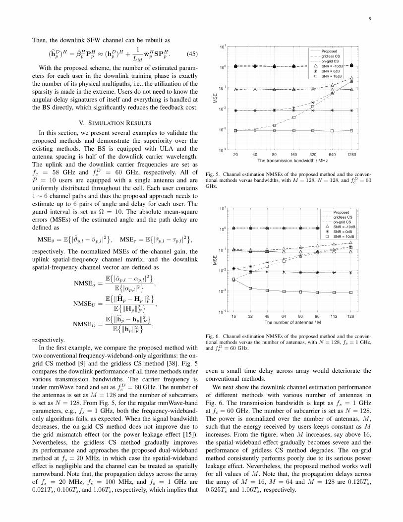
two conventional frequency-wideband-only algorithms: the on-grid CS method [9] and the gridless CS method [38]. Fig. 5compares the downlink performance of all three methods undervarious transmission bandwidths. The carrier frequency isunder mmWave band and set as fD

c = 60 GHz. The number ofthe antennas is set as M = 128 and the number of subcarriersis set as N = 128. From Fig. 5, for the regular mmWave-bandparameters, e.g., fs = 1 GHz, both the frequency-wideband-only algorithms fails, as expected. When the signal bandwidthdecreases, the on-grid CS method does not improve due tothe grid mismatch effect (or the power leakage effect [15]).Nevertheless, the gridless CS method gradually improvesits performance and approaches the proposed dual-widebandmethod at fs = 20 MHz, in which case the spatial-widebandeffect is negligible and the channel can be treated as spatiallynarrowband. Note that, the propagation delays across the arrayof fs = 20 MHz, fs = 100 MHz, and fs = 1 GHz are0.021Ts, 0.106Ts, and 1.06Ts, respectively, which implies that

20 40 80 160 320 640 1280The transmission bandwidth / MHz

10-4

10-3

10-2

10-1

100

101

MSE

Proposedgridless CSon-grid CSSNR = -10dBSNR = 0dBSNR = 10dB

Fig. 5. Channel estimation NMSEs of the proposed method and the conven-tional methods versus bandwidths, with M = 128, N = 128, and fD

c = 60GHz.

16 32 48 64 80 96 112 128The number of antennas / M

10-4

10-3

10-2

10-1

100

101

MSE

Proposedgridless CSon-grid CSSNR = -10dBSNR = 0dBSNR = 10dB

Fig. 6. Channel estimation NMSEs of the proposed method and the conven-tional methods versus the number of antennas, with N = 128, fs = 1 GHz,and fD

c = 60 GHz.

even a small time delay across array would deteriorate theconventional methods.

We next show the downlink channel estimation performanceof different methods with various number of antennas inFig. 6. The transmission bandwidth is kept as fs = 1 GHzat fc = 60 GHz. The number of subcarrier is set as N = 128.The power is normalized over the number of antennas, M ,such that the energy received by users keeps constant as Mincreases. From the figure, when M increases, say above 16,the spatial-wideband effect gradually becomes severe and theperformance of gridless CS method degrades. The on-gridmethod consistently performs poorly due to its serious powerleakage effect. Nevertheless, the proposed method works wellfor all values of M . Note that, the propagation delays acrossthe array of M = 16, M = 64 and M = 128 are 0.125Ts,0.525Ts and 1.06Ts, respectively.

10

0.85 1.9 3.6 28 37 6073The carrier frequency / GHz

10-4

10-3

10-2

10-1

100

101M

SE

Proposedgridless CSon-grid CSM=128, Bandwidth=20MHzM=128, Bandwidth=100MHzM=1024, Bandwidth=20MHzM=1024, Bandwidth=100MHz

Fig. 7. Channel estimation NMSEs of the proposed method and the conven-tional methods versus the carrier frequency, with N = 128 and SNR = 10dB.

Fig. 7 further compares the downlink performance of thethree methods under various transmission bandwidths and car-rier frequencies. The number of subcarriers is set as N = 128,and SNR is fixed in 10 dB. The number of the antennas is setas M = 128 and M = 1024, respectively. The transmissionbandwidth is set as fs = 20 MHz and fs = 100 MHz,respectively. From Fig. 7, even for the typical parameters,e.g., fs = 20 MHz at fc = 1.9 GHz, the spatial-widebandeffect is clearly observed when M is 128. Hence, for thesetypical system parameters, the traditional algorithms developedfor spatial-narrowband transmission cannot well estimate thechannels. Note that the maximum propagation delay acrossthe ULA under this parameter is 0.668Ts when M = 128, or5.38Ts when M = 1024, respectively.

From the above comparison, when the number of antennasin a ULA is fewer than 16, the spatial-wideband effect canbe ignored. It indicates that the conventional MIMO channelmodel is still applicable on a few current massive MIMOprototypes with the 8 × 8 and the 16 × 16 planar arrays atthose above-mentioned system parameters. Nevertheless, for amassive MIMO system with the antenna array containing morethan 16 antennas in one of dimension(s), the spatial-widebandeffect cannot be neglected and should be carefully treated.

Next, we demonstrate the uplink and the downlink perfor-mances of the proposed approach on different conditions.

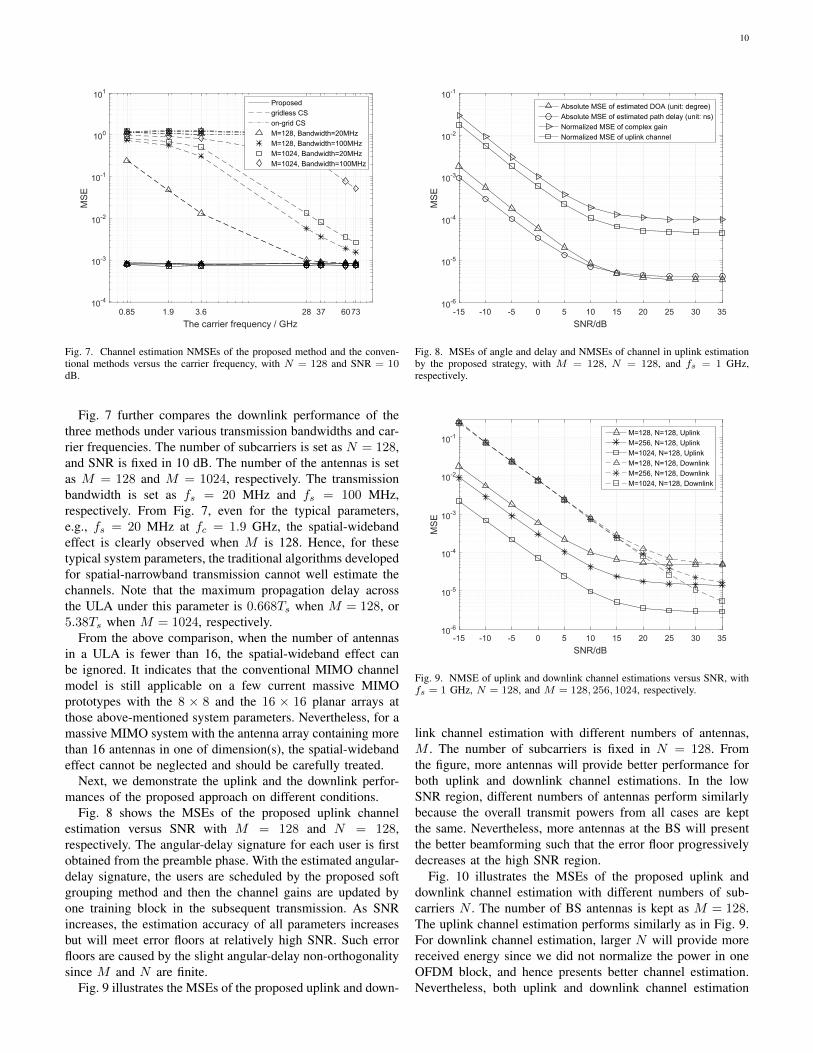
Fig. 8 shows the MSEs of the proposed uplink channelestimation versus SNR with M = 128 and N = 128,respectively. The angular-delay signature for each user is firstobtained from the preamble phase. With the estimated angular-delay signature, the users are scheduled by the proposed softgrouping method and then the channel gains are updated byone training block in the subsequent transmission. As SNRincreases, the estimation accuracy of all parameters increasesbut will meet error floors at relatively high SNR. Such errorfloors are caused by the slight angular-delay non-orthogonalitysince M and N are finite.

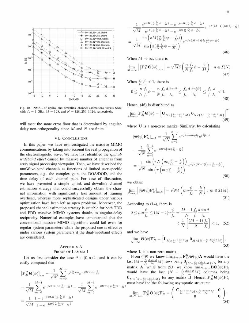
Fig. 9 illustrates the MSEs of the proposed uplink and down-

-15 -10 -5 0 5 10 15 20 25 30 35SNR/dB

10-6

10-5

10-4

10-3

10-2

10-1

MSE

Absolute MSE of estimated DOA (unit: degree)Absolute MSE of estimated path delay (unit: ns)Normalized MSE of complex gainNormalized MSE of uplink channel

Fig. 8. MSEs of angle and delay and NMSEs of channel in uplink estimationby the proposed strategy, with M = 128, N = 128, and fs = 1 GHz,respectively.

Fig. 9. NMSE of uplink and downlink channel estimations versus SNR, withfs = 1 GHz, N = 128, and M = 128, 256, 1024, respectively.

link channel estimation with different numbers of antennas,M . The number of subcarriers is fixed in N = 128. Fromthe figure, more antennas will provide better performance forboth uplink and downlink channel estimations. In the lowSNR region, different numbers of antennas perform similarlybecause the overall transmit powers from all cases are keptthe same. Nevertheless, more antennas at the BS will presentthe better beamforming such that the error floor progressivelydecreases at the high SNR region.

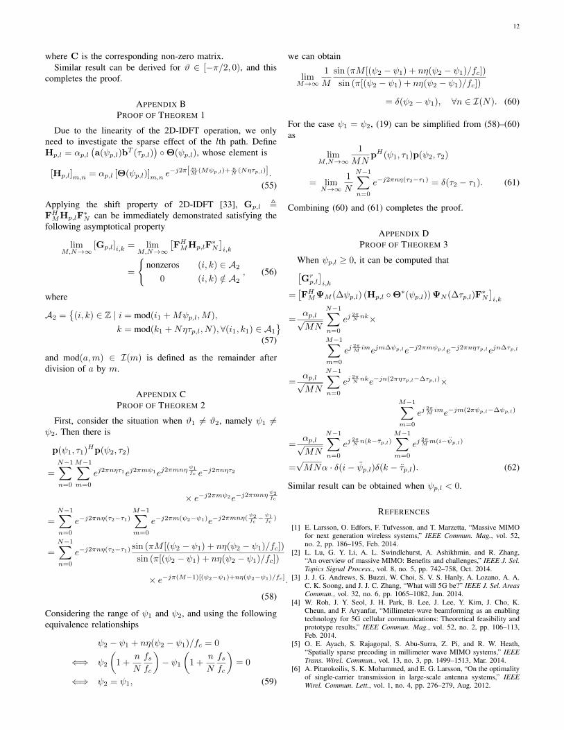
Fig. 10 illustrates the MSEs of the proposed uplink anddownlink channel estimation with different numbers of sub-carriers N . The number of BS antennas is kept as M = 128.The uplink channel estimation performs similarly as in Fig. 9.For downlink channel estimation, larger N will provide morereceived energy since we did not normalize the power in oneOFDM block, and hence presents better channel estimation.Nevertheless, both uplink and downlink channel estimation

11

Fig. 10. NMSE of uplink and downlink channel estimations versus SNR,with fs = 1 GHz, M = 128, and N = 128, 256, 1024, respectively.

will meet the same error floor that is determined by angular-delay non-orthogonality since M and N are finite.

VI. CONCLUSIONS

In this paper, we have re-investigated the massive MIMOcommunications by taking into account the real propagation ofthe electromagnetic wave. We have first identified the spatial-wideband effect caused by massive number of antennas fromarray signal processing viewpoint. Then, we have described themmWave-band channels as functions of limited user-specificparameters, e.g., the complex gain, the DOA/DOD, and thetime delay of each channel path. For ease of illustration,we have presented a simple uplink and downlink channelestimation strategy that could successfully obtain the chan-nel information with significantly less amount of trainingoverhead, whereas more sophisticated designs under variousoptimization have been left as open problems. Moreover, theproposed channel estimation strategy is suitable for both TDDand FDD massive MIMO systems thanks to angular-delayreciprocity. Numerical examples have demonstrated that theconventional massive MIMO algorithms could fail even forregular system parameters while the proposed one is effectiveunder various system parameters if the dual-wideband effectsare considered.

APPENDIX APROOF OF LEMMA 1

Let us first consider the case ϑ ∈ [0, π/2], and it can beeasily computed that

[FH

MΘ(ψ)]i,n

=1√M

M−1∑

m=0

ej2πM ime−j2πmnη ψ

fc

=1√M

M−1∑

m=0

e−j2πm(nη ψfc

− iM ) =

1√M

M−1∑

m=0

e−j2πm( nN

fsfc

ψ− iM )

=1√M

1− e−j2πM( nN

fsfc

ψ− iM )

1− e−j2π( nN

fsfc

ψ− iM )

=1√M

ejπM( nN

fsfc

ψ− iM ) − e−jπM( n

Nfsfc

ψ− iM )

ejπ(nN

fsfc

ψ− iM ) − e−jπ( n

Nfsfc

ψ− iM )

e−jπ(M−1)(nη ψfc

− iM )

=1√M

sin(πM( n

Nfsfcψ − i

M ))

sin(π( n

Nfsfcψ − i

M )) e−jπ(M−1)( n

Nfsfc

ψ− iM ).

(46)

When M → ∞, there is

limM→∞

∣∣∣[FH

MΘ(ψ)]i,n

∣∣∣ =√Mδ

(n

N

fsfc

ψ − i

M

), n ∈ I(N).

(47)

When fsfc

dλc

< 1, there is

0 ≤ n

N

fsfc

ψ =n

N

fsfc

d sinϑ

λc≤ fs

fc

d sin(ϑ)

λc≤ fs

fc

d

λc< 1.

(48)

Hence, (46) is distributed as

limM→∞

FHMΘ(ψ) =

[UN×( fs

fcd sinϑ

λcM) 0N×(M− fs

fcd sinϑ

λcM)

]T

(49)

where U is a non-zero matrix. Similarly, by calculating

[Θ(ψ)F∗N ]m,k =

1√N

N−1∑

n=0

e−j2πmnη ψfc ej

2πN nk

=1√N

N−1∑

n=0

e−j2πn(mη ψfc

− kN )

=1√N

sin(πN

(mη ψ

fc− k

N

))

sin(π(mη ψ

fc− k

N

)) e−jπ(N−1)(mη ψfc

− kN ),

(50)

we obtain

limN→∞

∣∣∣ [Θ(ψ)F∗N ]m,k

∣∣∣ =√Nδ

(mη

ψ

fc− k

N

), m ∈ I(M).

(51)

According to (14), there is

0 ≤ mηψ

fc≤ (M − 1)η

ψ

fc=

M − 1

N

fsfc

d sinϑ

λc

<1

N

[(M − 1)

2

fsfc

]< 1, (52)

and we have

limN→∞

Θ(ψ)F∗N =

[LM× fs

fcd sinϑ

λcM 0M×(N− fs

fcd sinϑ

λcM)

],

(53)

where L is a non-zero matrix.From (49) we know limM→∞ FH

MΘ(ψ)A would have thelast (M− fs

fcd sinϑλc

M) rows being 0(M− fsfc

d sinϑλc

M)×N for anymatrix A, while from (53) we know limN→∞ BΘ(ψ)F∗

N

would have the last (N − fsfc

d sinϑλc

M) columns being0M×(N− fs

fcd sinϑ

λcM) for any matrix B. Hence, FH

MΘ(ψ)F∗N

must have the the following asymptotic structure:

limM,N→∞

FHMΘ(ψ)F∗

N =

(C fs

fcd sinϑ

λcM× fs

fcd sinϑ

λcM 0

0 0

),

(54)

12

where C is the corresponding non-zero matrix.Similar result can be derived for ϑ ∈ [−π/2, 0), and this

completes the proof.

APPENDIX BPROOF OF THEOREM 1

Due to the linearity of the 2D-IDFT operation, we onlyneed to investigate the sparse effect of the lth path. DefineHp,l = αp,l

(a(ψp,l)b

T (τp,l))◦Θ(ψp,l), whose element is

[Hp,l]m,n = αp,l [Θ(ψp,l)]m,n e−j2π[m

M (Mψp,l)+nN (Nητp,l)].

(55)

Applying the shift property of 2D-IDFT [33], Gp,l �FH

MHp,lF∗N can be immediately demonstrated satisfying the

following asymptotical property

limM,N→∞

[Gp,l]i,k = limM,N→∞

[FH

MHp,lF∗N

]i,k

=

{nonzeros (i, k) ∈ A2

0 (i, k) /∈ A2

, (56)

where

A2 ={(i, k) ∈ Z | i = mod(i1 +Mψp,l,M),

k = mod(k1 +Nητp,l, N), ∀(i1, k1) ∈ A1

}

(57)

and mod(a,m) ∈ I(m) is defined as the remainder afterdivision of a by m.

APPENDIX CPROOF OF THEOREM 2

First, consider the situation when ϑ1 �= ϑ2, namely ψ1 �=ψ2. Then there is

p(ψ1, τ1)Hp(ψ2, τ2)

=N−1∑

n=0

M−1∑

m=0

ej2πnητ1ej2πmψ1ej2πmnηψ1fc e−j2πnητ2

× e−j2πmψ2e−j2πmnηψ2fc

=N−1∑

n=0

e−j2πnη(τ2−τ1)M−1∑

m=0

e−j2πm(ψ2−ψ1)e−j2πmnη(ψ2fc

−ψ1fc

)

=N−1∑

n=0

e−j2πnη(τ2−τ1)sin (πM [(ψ2 − ψ1) + nη(ψ2 − ψ1)/fc])

sin (π[(ψ2 − ψ1) + nη(ψ2 − ψ1)/fc])

× e−jπ(M−1)[(ψ2−ψ1)+nη(ψ2−ψ1)/fc].

(58)

Considering the range of ψ1 and ψ2, and using the followingequivalence relationships

ψ2 − ψ1 + nη(ψ2 − ψ1)/fc = 0

⇐⇒ ψ2

(1 +

n

N

fsfc

)− ψ1

(1 +

n

N

fsfc

)= 0

⇐⇒ ψ2 = ψ1, (59)

we can obtain

limM→∞

1

M

sin (πM [(ψ2 − ψ1) + nη(ψ2 − ψ1)/fc])

sin (π[(ψ2 − ψ1) + nη(ψ2 − ψ1)/fc])

= δ(ψ2 − ψ1), ∀n ∈ I(N). (60)

For the case ψ1 = ψ2, (19) can be simplified from (58)–(60)as

limM,N→∞

1

MNpH(ψ1, τ1)p(ψ2, τ2)

= limN→∞

1

N

N−1∑

n=0

e−j2πnη(τ2−τ1) = δ(τ2 − τ1). (61)

Combining (60) and (61) completes the proof.

APPENDIX DPROOF OF THEOREM 3

When ψp,l ≥ 0, it can be computed that[Gr

p,l

]i,k

=[FH

MΨM (Δψp,l) (Hp,l ◦Θ∗(ψp,l))ΨN (Δτp,l)F∗N

]i,k

=αp,l√MN

N−1∑

n=0

ej2πN nk×

M−1∑

m=0

ej2πM imejmΔψp,le−j2πmψp,le−j2πnητp,lejnΔτp,l

=αp,l√MN

N−1∑

n=0

ej2πN nke−jn(2πητp,l−Δτp,l)×

M−1∑

m=0

ej2πM ime−jm(2πψp,l−Δψp,l)

=αp,l√MN

N−1∑

n=0

ej2πN n(k−τp,l)

M−1∑

m=0

ej2πM m(i−ψp,l)

=√MNα · δ(i− ψp,l)δ(k − τp,l). (62)

Similar result can be obtained when ψp,l < 0.

REFERENCES

[1] E. Larsson, O. Edfors, F. Tufvesson, and T. Marzetta, “Massive MIMOfor next generation wireless systems,” IEEE Commun. Mag., vol. 52,no. 2, pp. 186–195, Feb. 2014.

[2] L. Lu, G. Y. Li, A. L. Swindlehurst, A. Ashikhmin, and R. Zhang,“An overview of massive MIMO: Benefits and challenges,” IEEE J. Sel.Topics Signal Process., vol. 8, no. 5, pp. 742–758, Oct. 2014.

[3] J. J. G. Andrews, S. Buzzi, W. Choi, S. V. S. Hanly, A. Lozano, A. A.C. K. Soong, and J. J. C. Zhang, “What will 5G be?” IEEE J. Sel. AreasCommun., vol. 32, no. 6, pp. 1065–1082, Jun. 2014.

[4] W. Roh, J. Y. Seol, J. H. Park, B. Lee, J. Lee, Y. Kim, J. Cho, K.Cheun, and F. Aryanfar, “Millimeter-wave beamforming as an enablingtechnology for 5G cellular communications: Theoretical feasibility andprototype results,” IEEE Commun. Mag., vol. 52, no. 2, pp. 106–113,Feb. 2014.

[5] O. E. Ayach, S. Rajagopal, S. Abu-Surra, Z. Pi, and R. W. Heath,“Spatially sparse precoding in millimeter wave MIMO systems,” IEEETrans. Wirel. Commun., vol. 13, no. 3, pp. 1499–1513, Mar. 2014.

[6] A. Pitarokoilis, S. K. Mohammed, and E. G. Larsson, “On the optimalityof single-carrier transmission in large-scale antenna systems,” IEEEWirel. Commun. Lett., vol. 1, no. 4, pp. 276–279, Aug. 2012.

13

[7] Z. Gao, L. Dai, C. Yuen, and Z. Wang, “Asymptotic orthogonality anal-ysis of time-domain sparse massive MIMO channels,” IEEE Commun.Lett., vol. 19, no. 10, pp. 1826–1829, Oct. 2015.

[8] T. L. Marzetta, “Noncooperative cellular wireless with unlimited num-bers of base station antennas,” IEEE Trans. Wirel. Commun., vol. 9, no.11, pp. 3590–3600, Nov. 2010.

[9] Z. Chen and C. Yang, “Pilot decontamination in wideband massiveMIMO systems by exploiting channel sparsity,” IEEE Trans. Wirel.Commun., vol. 15, no. 7, pp. 5087–5100, Jul. 2016.

[10] R. R. Muller, L. Cottatellucci, and M. Vehkapera, “Blind pilot decontam-ination,” IEEE J. Sel. Top. Signal Process., vol. 8, no. 5, pp. 773–786,Oct. 2014.

[11] H. Yin, D. Gesbert, M. Filippou, and Y. Liu, “A coordinated approachto channel estimation in large-scale multiple-antenna systems,” IEEE J.Sel. Areas Commun., vol. 31, no. 2, pp. 264–273, Feb. 2013.

[12] J. Guey and L. Larsson, “Modeling and evaluation of MIMO systemsexploiting channel reciprocity in TDD mode,” IEEE 60th Veh. Technol.Conf., 2004. (VTC2004-Fall), 2004, pp. 4265–4269.

[13] J. Choi, D. J. Love, and P. Bidigare, “Downlink training techniques forFDD massive MIMO systems: Open-loop and closed-loop training withmemory,” IEEE J. Sel. Top. Signal Process., vol. 8, no. 5, Oct. 2014,pp. 802–814.

[14] Y. Han, J. Lee, and D. J. Love, “Compressed sensing-aided downlinkchannel training for FDD massive MIMO systems,” IEEE Trans. Com-mun., vol. 65, no. 7, pp. 2852–2862, Jul. 2017.

[15] H. Xie, F. Gao, S. Zhang, and S. Jin, “A unified transmission strategy forTDD/FDD massive MIMO systems with spatial basis expansion model,”IEEE Trans. Veh. Technol., vol. 66, no. 4, pp. 3170–3184, Apr. 2017.

[16] J. Brady, N. Behdad, and A. M. Sayeed, “Beamspace MIMO formillimeter-wave communications: System architecture, modeling, anal-ysis, and measurements,” IEEE Trans. Antennas Propag., vol. 61, no. 7,pp. 3814–3827, Jul. 2013.

[17] A. Adhikary, E. Al Safadi, M. K. Samimi, R. Wang, G. Caire, T. S.Rappaport, and A. F. Molisch, “Joint spatial division and multiplexingfor mm-Wave channels,” IEEE J. Sel. Areas Commun., vol. 32, no. 6,pp. 1239–1255, Jun. 2014.

[18] Z. Gao, L. Dai, D. Mi, Z. Wang, M. A. Imran, and M. Z. Shakir,“MmWave massive-MIMO-based wireless backhaul for the 5G ultra-dense network,” IEEE Wirel. Commun., vol. 22, no. 5, pp. 13–21, Oct.2015.

[19] J. C. Chen, “Hybrid beamforming with discrete phase shifters formillimeter-wave massive MIMO systems,” IEEE Trans. Veh. Technol.,vol. 66, no. 8, pp. 7604–7608, Aug. 2017.

[20] Z. Gao, C. Hu, L. Dai, and Z. Wang, “Channel estimation for millimeter-wave massive MIMO with hybrid precoding over frequency-selectivefading channels,” IEEE Commun. Lett., vol. 20, no. 6, pp. 1259–1262,Jun. 2016.

[21] S. Han, C.-l. I, Z. Xu, and C. Rowell, “Large-scale antenna systemswith hybrid analog and digital beamforming for millimeter wave 5G,”IEEE Commun. Mag., vol. 53, no. 1, pp. 186–194, Jan. 2015.

[22] F. Sohrabi and W. Yu, “Hybrid digital and analog beamforming designfor large-scale antenna arrays,” IEEE J. Sel. Top. Signal Process., vol.10, no. 3, pp. 501–513, Apr. 2016.

[23] T.-S. Chu and H. Hashemi, “True-time-delay-based multi-beam arrays,”IEEE Trans. Microw. Theory Tech., vol. 61, no. 8, pp. 3072–3082, Aug.2013.

[24] J. H. Brady and A. M. Sayeed, “Wideband communication with high-dimensional arrays: New results and transceiver architectures,” in 2015IEEE Int. Conf. Commun. Work. (ICCW), London, 2015, pp. 1042-1047.

[25] B. Wang, F. Gao, S. Jin, H. Lin, and G. Y. Li, “Spatial-wideband effectin massive MIMO systems,” in Proc. IEEE APCC, 2017, to appear.

[26] B. Friedlander and A. J. Weiss, “Direction finding for wid-band signalsusing an interpolated array,” IEEE Trans. Signal Process., vol. 41, no.4, pp. 1618–1634, Apr. 1993.

[27] Y. S. Yoon, L. M. Kaplan, and J. H. McClellan, “TOPS: New DOAestimator for wideband signals,” IEEE Trans. Signal Process., vol. 54,no. 6 I, pp. 1977–1989, Jun. 2006.

[28] D. Tse and P. Viswanath, Fundamentals of Wireless Communication,Cambridge University Press, 2005.

[29] R. W. Heath, N. Gonzalez-Prelcic, S. Rangan, W. Roh, and A. M.Sayeed, “An overview of signal processing techniques for millimeterwave MIMO systems,” IEEE J. Sel. Top. Signal Process., vol. 10, no.3, pp. 436–453, Apr. 2016.

[30] J. A. Zhang, X. Huang, V. Dyadyuk, and Y. J. Guo, “Massive hybridantenna array for millimeter-wave cellular communications,” IEEE Wire-less Commun., vol. 22, no. 1, pp. 79–87, Feb. 2015.

[31] H. Xie, F. Gao, and S. Jin, “An overview of low-rank channel estimationfor massive MIMO systems,” IEEE Access, vol. 4, pp. 7313–7321, 2016.

[32] M. Cai, K. Gao, D. Nie, B. Hochwald, and J. N. Laneman, “Effectof wideband beam squint on codebook design in phased-array wirelesssystems,” in 2016 IEEE Glob. Commun. Conf. (GLOBECOM), Wash-ington, DC, 2016, pp. 1–6.

[33] S. K. Mitra, Digital Signal Processing: A Computer-based Approach.,McGraw-Hill/Irwin, 2005.

[34] X. Ren, W. Chen, and M. Tao, “Position-based compressed channelestimation and pilot design for high-mobility OFDM systems,” IEEETrans. Veh. Technol., vol. 64, no. 5, pp. 1918–1929, May. 2015.

[35] J. W. Choi, B. Shim, and S. H. Chang, “Downlink pilot reduction formassive MIMO systems via compressed sensing,” IEEE Commun. Lett.,vol. 19, no. 11, pp. 1889–1892, Nov. 2015.

[36] Y. Pati, R. Rezaiifar, and P. Krishnaprasad, “Orthogonal matchingpursuit: recursive function approximation with applications to waveletdecomposition,” in Proc. 27th Asilomar Conf. Signals, Syst. Comput.,Pacific Grove, CA, 1993, pp. 40-44.

[37] A. Beck and M. Teboulle, “A fast iterative shrinkage-thresholdingalgorithm,” Soc. Ind. Appl. Math. J. Imaging Sci., vol. 2, no. 1, pp.183–202, Mar. 2009.

[38] J. Fang, F. Wang, Y. Shen, H. Li, and R. S. Blum, “Super-resolutioncompressed sensing for line spectral estimation: An Iterative ReweightedApproach,” IEEE Trans. Signal Process., vol. 64, no. 18, pp. 4649–4662,Sep. 2016.

[39] I. Barhumi, G. Leus, and M. Moonen, “Optimal training design forMIMO OFDM systems in mobile wireless channels,” IEEE Trans. SignalProcess., vol. 51, no. 6, pp. 1615–1624, Jun. 2003.

[40] J. Wang, P. Ding, M. Zoltowski, and D. Love, “Space-time codingand beamforming with partial channel state information,” in GlobalTelecommunications Conference, 2005. GLOBECOM ’05. IEEE, vol. 5,December 2005, pp. 3149–3153.

[41] A. Alkhateeb, O. El Ayach, G. Leus, and R. Heath, “Hybrid precodingfor millimeter wave cellular systems with partial channel knowledge,” inInformation Theory and Applications Workshop (ITA), 2013, February2013, pp. 1–5.

[42] Y. Ramadan, A. Ibrahim, and M. Khairy, “Minimum outage RF beam-forming for millimeter wave MISO-OFDM systems,” in Wireless Com-munications and Networking Conference (WCNC), 2015 IEEE, March2015, pp. 557–561.

[43] Y. J. Bultitude, and T. Rautiainen, “IST-4-027756 WINNER II D1. 1.2V1. 2 WINNER II Channel Models,” 2007.

[44] METIS, Mobile wireless communications Enablers for the Twenty-twenty Information Society, EU 7th Framework Programme project, vol.6. ICT-317669-METIS.