Embed Size (px)
Citation preview
Spatial Analysis and Modeling (GIST 4302/5302)
Guofeng CaoDepartment of Geosciences
Texas Tech University
Representation of Spatial Data

Representation of Spatial Data Models
• Object-based model: treats the space as populated by discrete, identifiable entities each with a geospatial reference– Buildings or roads fit into this view– GIS Softwares: ArcGIS
• Field-based model: treats geographic information as collections of spatial distributions– Distribution may be formalized as a mathematical function from a spatial
framework to an attribute domain– Patterns of topographic altitudes, rainfall, and temperature fit neatly into
this view.– GIS Software: Grass
Object-based Approach
Entity
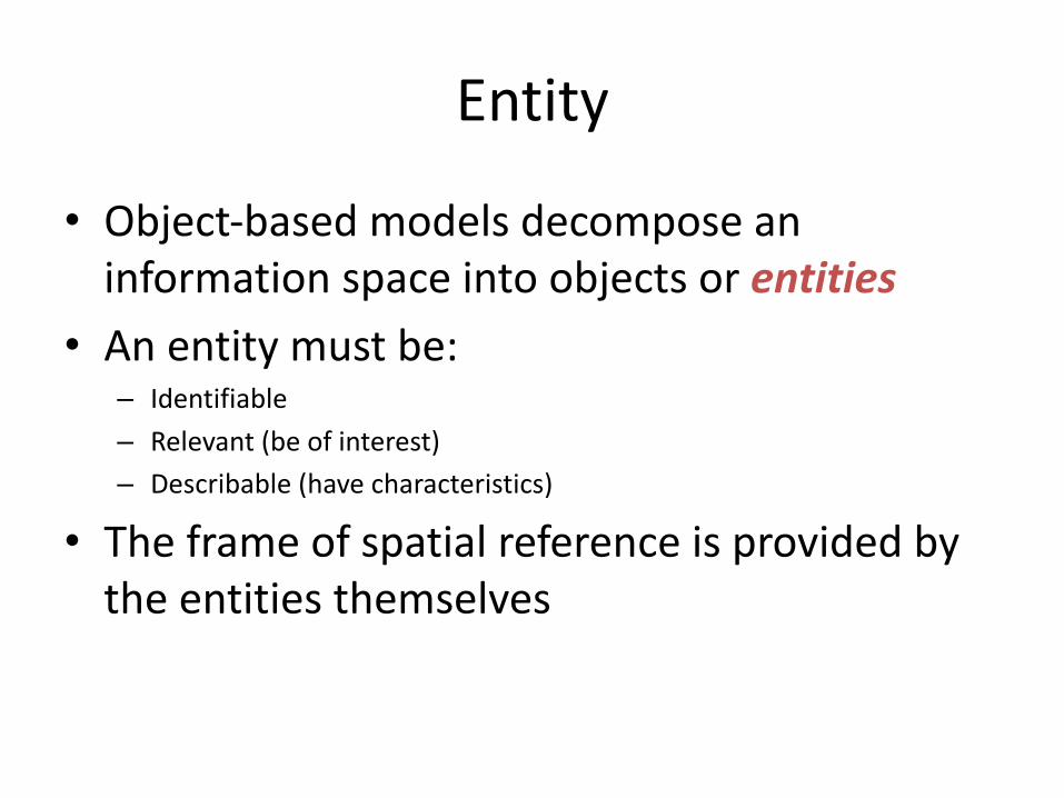
• Object-based models decompose an information space into objects or entities
• An entity must be:– Identifiable– Relevant (be of interest)– Describable (have characteristics)
• The frame of spatial reference is provided by the entities themselves

Example: House object
Has several attributes, such as registration date, address, owner and boundary, which are themselves objects
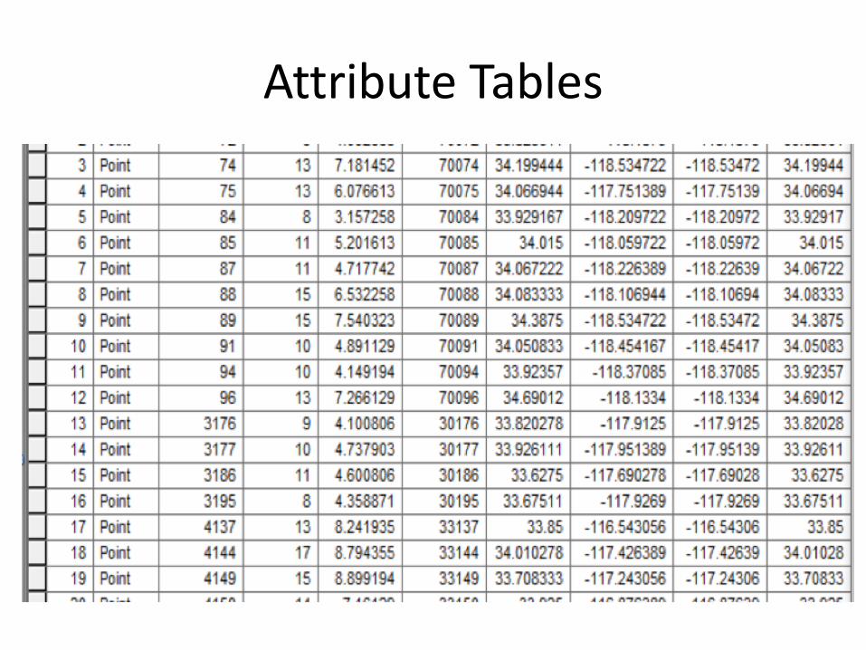
Attribute Tables

Attribute Tables
• Basic operators on attribute tables– Selection: picking certain rows– Projection: picking certain columns– Join: compositions of relations

Project Operator• The project operator is unary– It outputs a new relation that has a subset of
attributes– Identical tuples in the output relation are
coalesced
Relation Sells:bar beer priceChimy’s Bud 2.50Chimy’s Miller 2.75Cricket’s Bud 2.50Cricket’s Miller 3.00
Prices := PROJbeer,price(Sells):beer priceBud 2.50Miller 2.75Miller 3.00

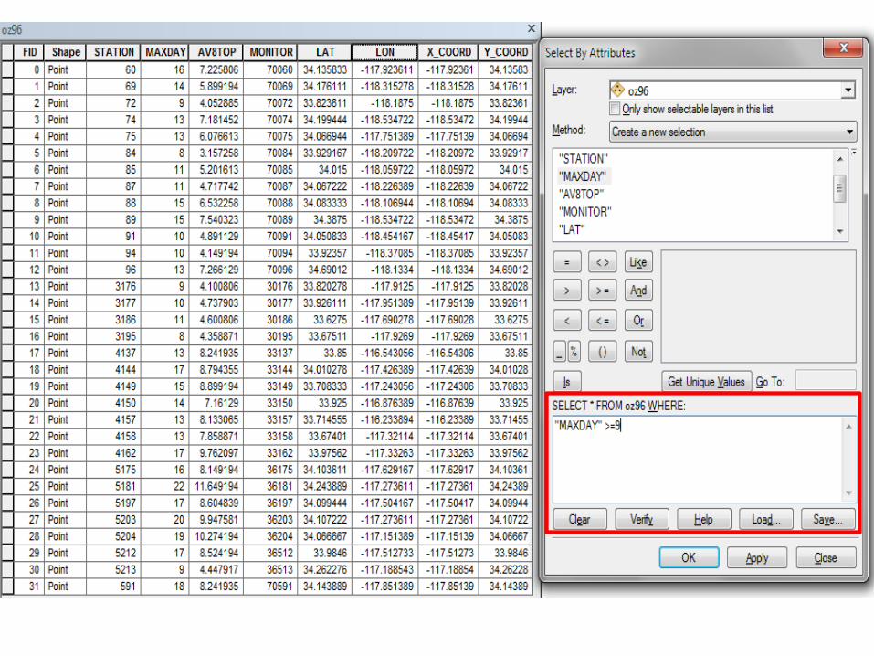
Select Operator• The select operator is unary
– It outputs a new relation that has a subset of tuples – A condition specifies those tuples that are required
Relation Sells:bar beer priceChimy’s Bud 2.50Chimy’s Miller 2.75Cricket’s Bud 2.50Cricket’s Miller 3.00
ChimyMenu := SELECTbar=“Chimy’s”(Sells):bar beer priceChimy’s Bud 2.50Chimy’s Miller 2.75

Join Operator
• The join operator is binary– It outputs the combined relation where tuples agree on a specified
attribute (natural join)Sells(bar, beer, price ) Bars(bar, address)
Chimy’s Bud 2.50 Chimy’s 2417 Broadway St.Chimy’s Miller 2.75 Cricekt’s 2412 Broadway St.Cricket’s Bud 2.50Cricket’s Coors 3.00
BarInfo := Sells JOIN BarsNote Bars.name has become Bars.bar to make the naturaljoin “work.”
BarInfo(bar, beer, price, address )
Chimy’s Bud 2.50 2417 Broadway St.Chimy’s Milller 2.75 2417 Broadway St.Cricket’s Bud 2.50 2412 Broadway St.Cricket’s Coors 3.00 2412 Broadway St.
Join Operator
• Join is the most time-consuming of all relational operators to compute– In general, relational operators may not be arbitrarily
reordered (left join, right join)– Query optimization aims to find an efficient way of
processing queries, for example reordering to produce equivalent but more efficient queries
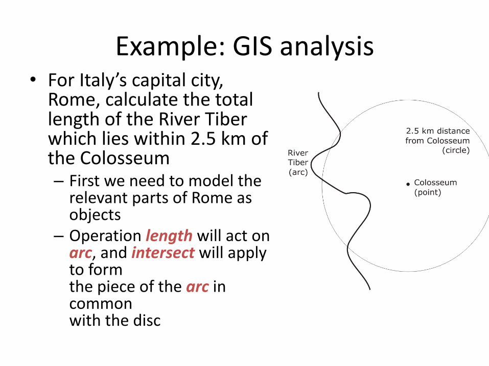
Example: GIS analysis• For Italy’s capital city,
Rome, calculate the total length of the River Tiber which lies within 2.5 km of the Colosseum– First we need to model the
relevant parts of Rome as objects
– Operation length will act on arc, and intersect will apply to form the piece of the arc in common with the disc
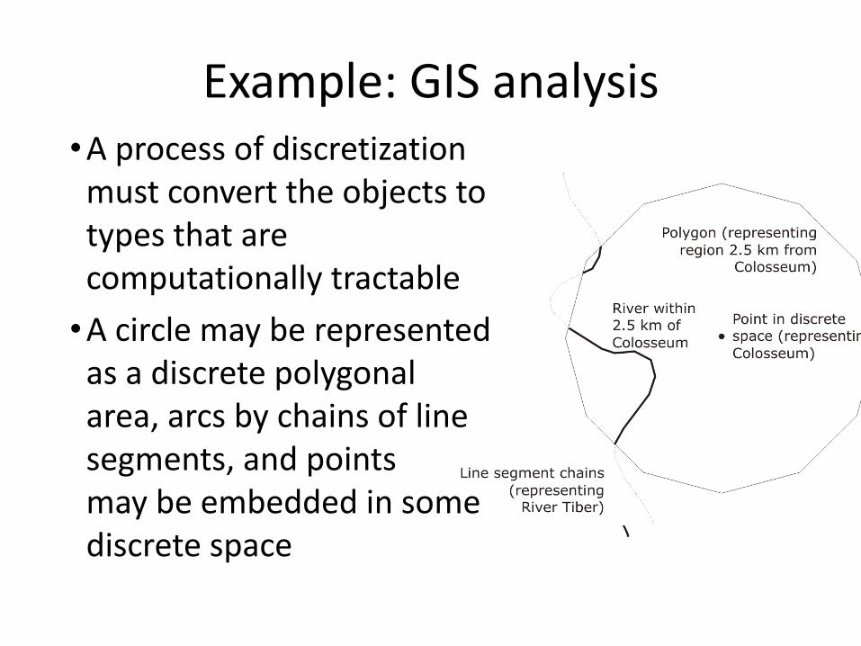
Example: GIS analysis•A process of discretization
must convert the objects to types that are computationally tractable•A circle may be represented
as a discrete polygonal area, arcs by chains of line segments, and pointsmay be embedded in some discrete space
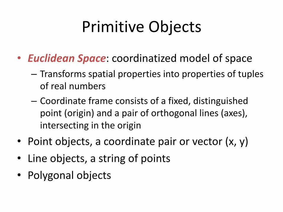
Primitive Objects
• Euclidean Space: coordinatized model of space– Transforms spatial properties into properties of tuples
of real numbers– Coordinate frame consists of a fixed, distinguished
point (origin) and a pair of orthogonal lines (axes), intersecting in the origin
• Point objects, a coordinate pair or vector (x, y)• Line objects, a string of points• Polygonal objects

Polygonal objects
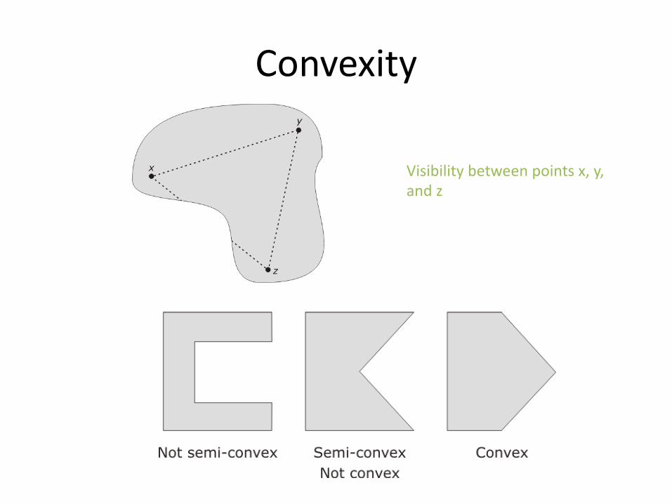
Convexity
Visibility between points x, y, and z

Example: Triangulation
• Every simple polygon has a triangulation. Any triangulation of a simple polygon with n vertices consists of exactly n – 2 triangles
• Art Gallery Problem– How many cameras are needed to guard a gallery and how should they be
placed?– Upper bound N/3

Related: Convex Hull
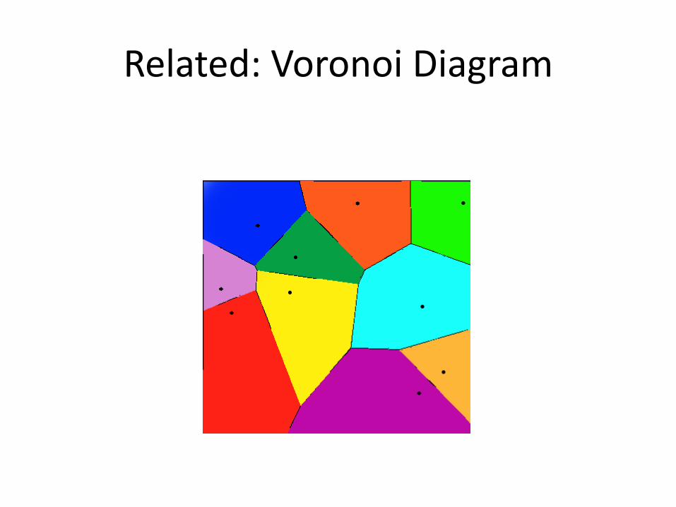
Related: Voronoi Diagram
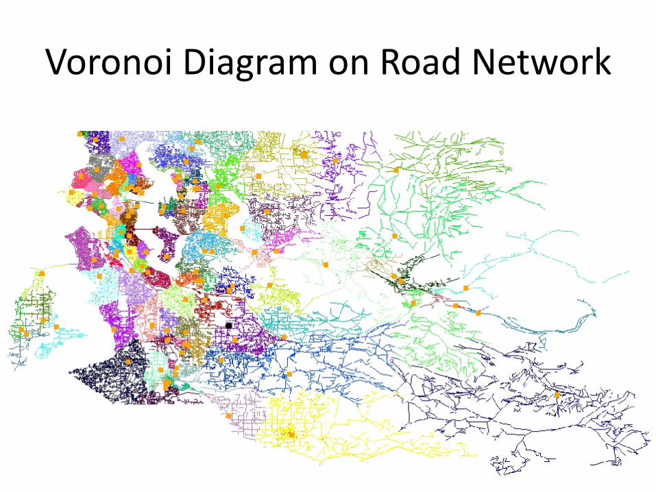
Voronoi Diagram on Road Network
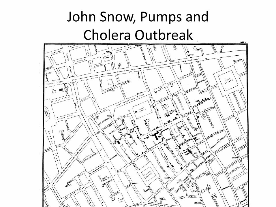
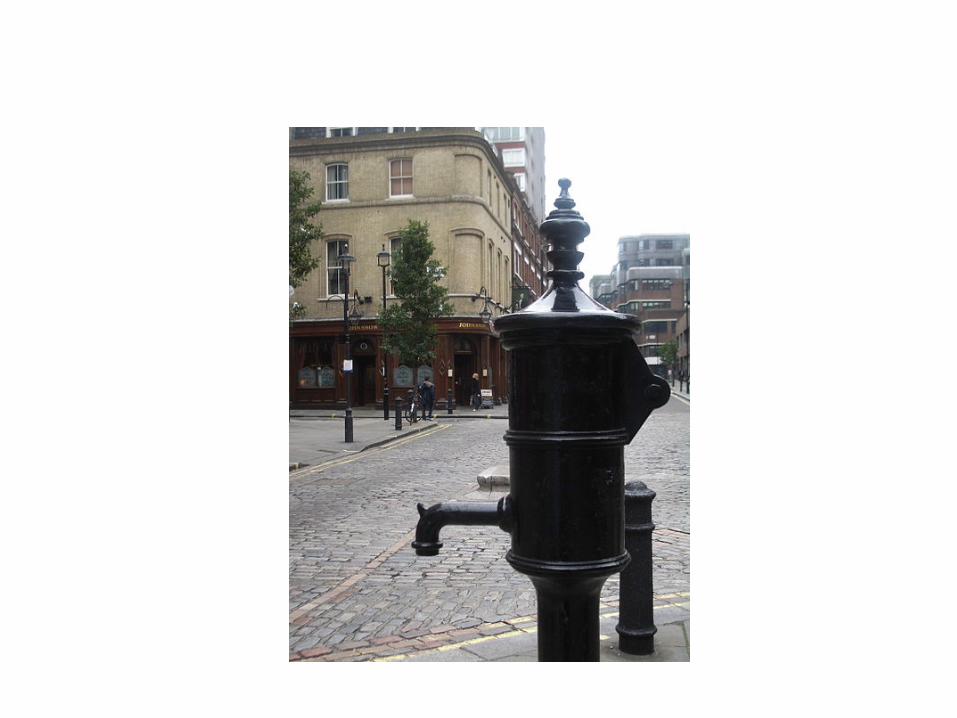
John Snow, Pumps and Cholera Outbreak

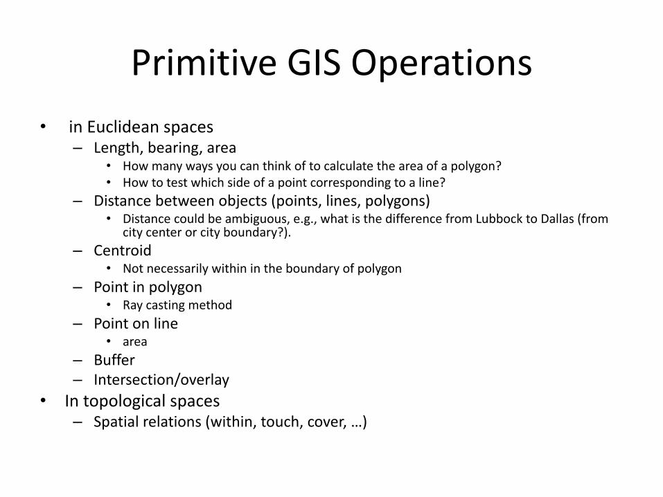
Primitive GIS Operations• in Euclidean spaces
– Length, bearing, area• How many ways you can think of to calculate the area of a polygon?• How to test which side of a point corresponding to a line?
– Distance between objects (points, lines, polygons)• Distance could be ambiguous, e.g., what is the difference from Lubbock to Dallas (from
city center or city boundary?).– Centroid
• Not necessarily within in the boundary of polygon– Point in polygon
• Ray casting method– Point on line
• area– Buffer– Intersection/overlay
• In topological spaces– Spatial relations (within, touch, cover, …)
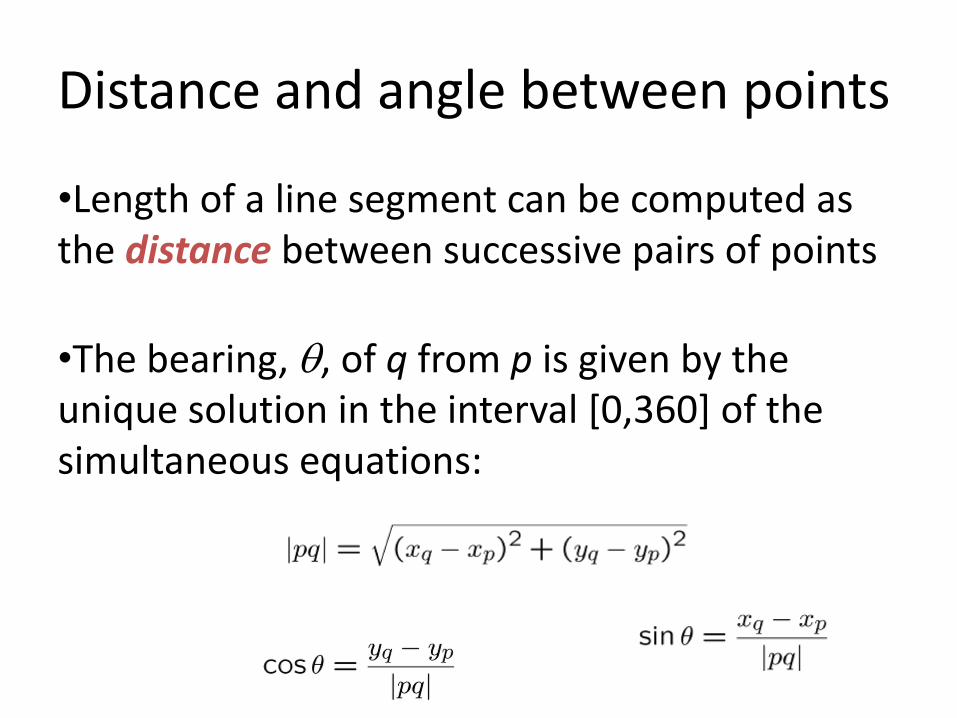
Distance and angle between points
•Length of a line segment can be computed as the distance between successive pairs of points
•The bearing, q, of q from p is given by the unique solution in the interval [0,360] of the simultaneous equations:

Distance from point to line•from a point to a line implies minimum distance•For a straight line segment, distance computation depends on whether p is in middle(l) or end(l)•For a polyline, distance to each line segment must be calculated
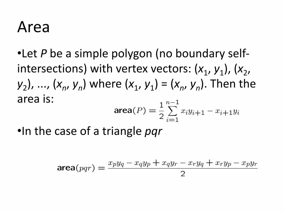
Area•Let P be a simple polygon (no boundary self-intersections) with vertex vectors: (x1, y1), (x2, y2), ..., (xn, yn) where (x1, y1) = (xn, yn). Then the area is:
•In the case of a triangle pqr
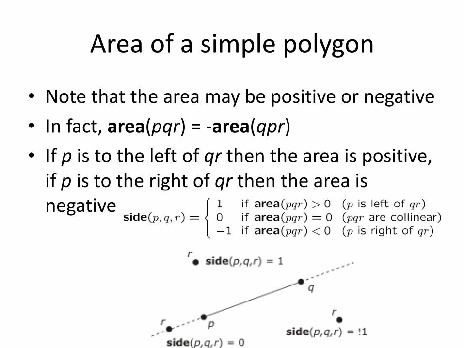
Area of a simple polygon
• Note that the area may be positive or negative• In fact, area(pqr) = -area(qpr)• If p is to the left of qr then the area is positive,
if p is to the right of qr then the area is negative

Centroid
•The centroid of a polygon (or center of gravity) of a (simple) polygonal object (P = (x1, y1), (x2, y2), ..., (xn, yn), where (x1, y1) = (xn, yn)) is the point at which it would balance if it were cut out of a sheet of material of uniform density:

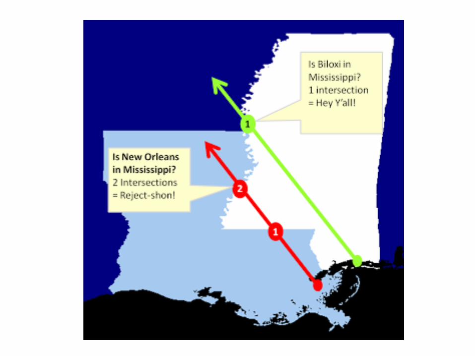
Point in polygon• Determining whether a point is inside a polygon is one of
the most fundamental operations in a spatial database• Semi-line method (ray casting) : checks for odd or even
numbers of intersections of a semi-line with polygon• Winding method: sums bearings from point to polygon
vertices

Primitive GIS operations: Overlay
• Union• Intersect• Erase• Identity• Update• Spatial Join• Symmetrical Difference
Overlay
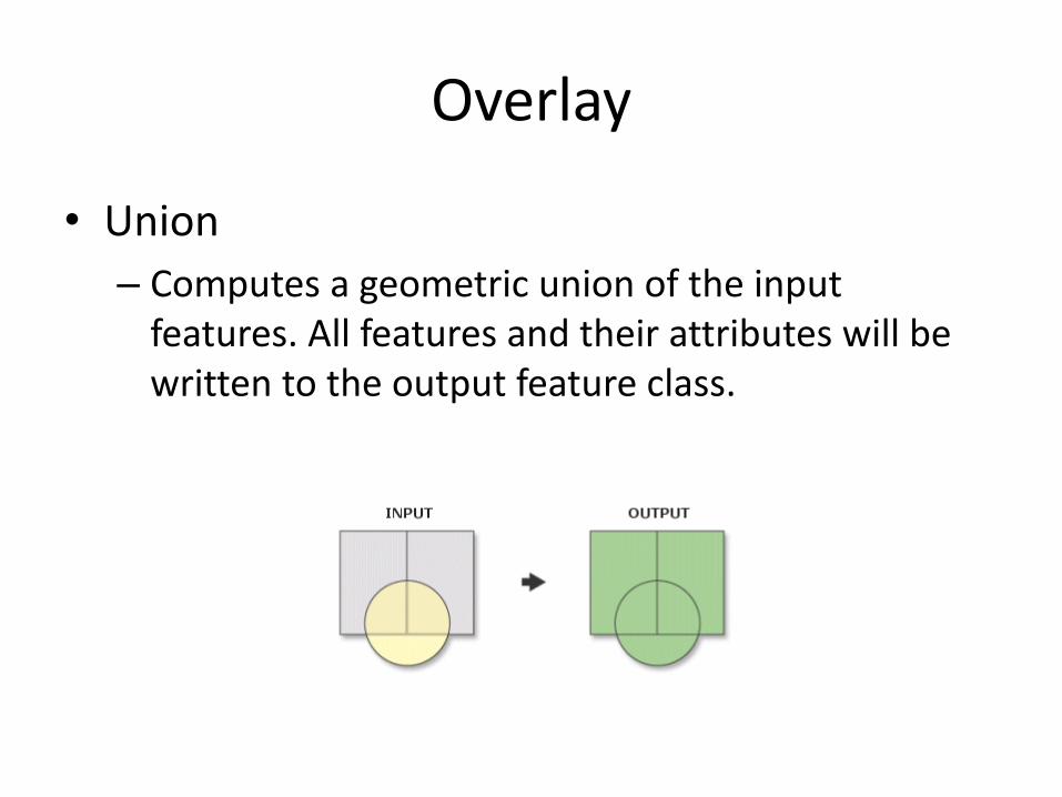
• Union– Computes a geometric union of the input
features. All features and their attributes will be written to the output feature class.

Overlay
• Intersect– Computes a geometric intersection of the input
features. Features or portions of features which overlap in all layers and/or feature classes will be written to the output feature class.
Overlay
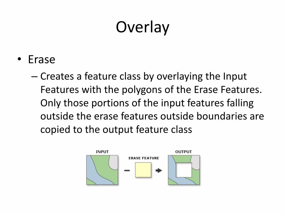
• Erase– Creates a feature class by overlaying the Input
Features with the polygons of the Erase Features. Only those portions of the input features falling outside the erase features outside boundaries are copied to the output feature class
Overlay
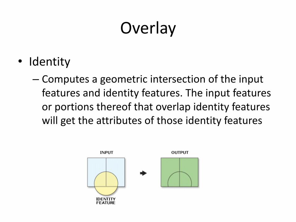
• Identity– Computes a geometric intersection of the input
features and identity features. The input features or portions thereof that overlap identity features will get the attributes of those identity features
Overlay
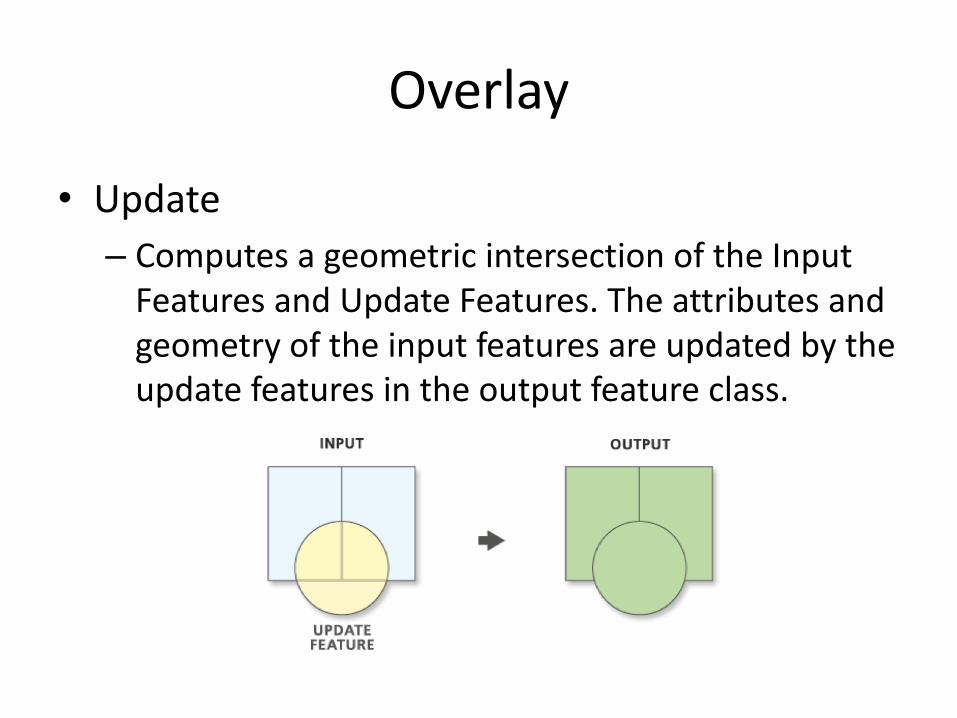
• Update– Computes a geometric intersection of the Input
Features and Update Features. The attributes and geometry of the input features are updated by the update features in the output feature class.
Overlay
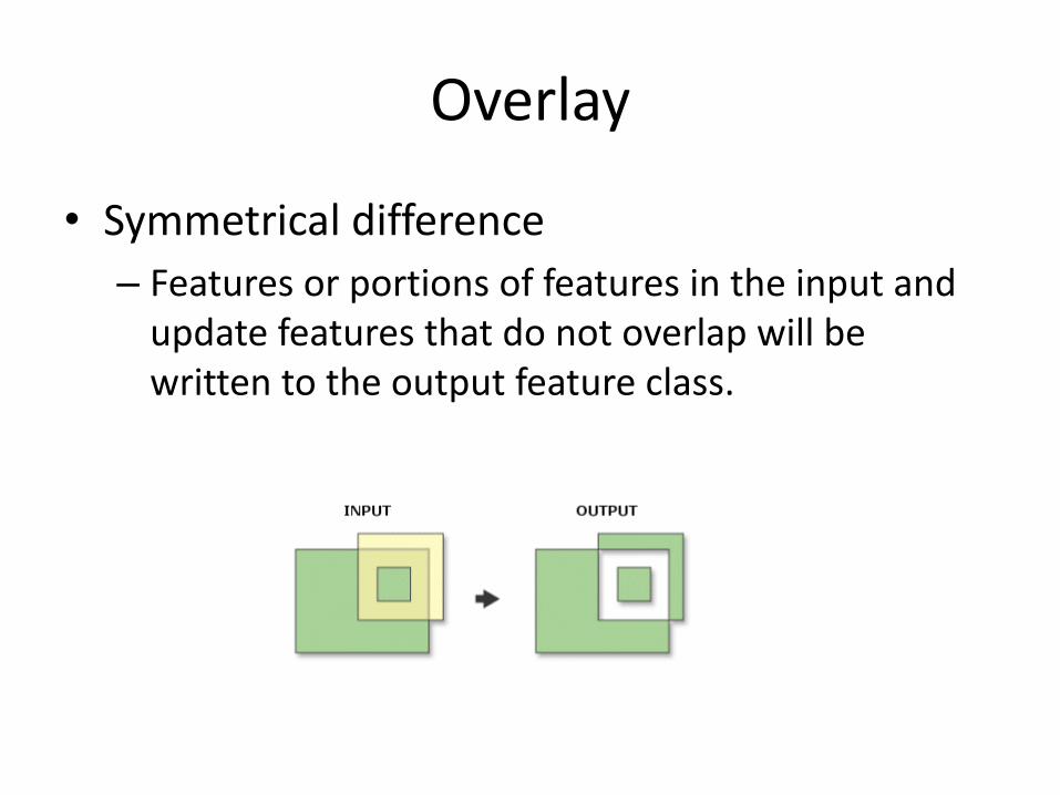
• Symmetrical difference– Features or portions of features in the input and
update features that do not overlap will be written to the output feature class.
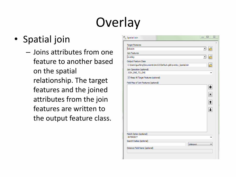
Overlay• Spatial join– Joins attributes from one
feature to another based on the spatial relationship. The target features and the joined attributes from the join features are written to the output feature class.
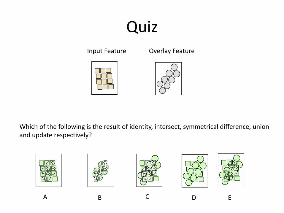
QuizInput Feature Overlay Feature
Which of the following is the result of identity, intersect, symmetrical difference, union and update respectively?
A B C D E
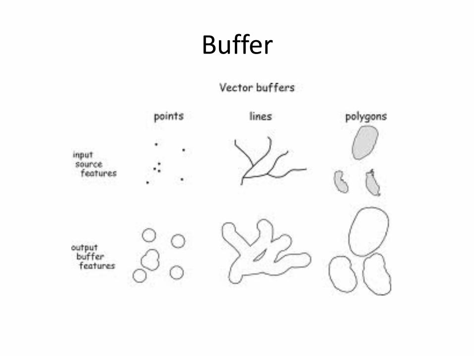
Buffer

• Primitive operators– you might already realized that these primitive
operators are often used collaboratively with each other, and other analytical methods (e.g., dissolve, surface analysis, interpolation) that we will introduce in the coming lectures.

Topological spatial operations: spatial relationship
• Object types with an assumed underlying topology are point, arc, loop and area
• Operations:– boundary, interior, closure and connected are defined
in the usual manner– components returns the set of maximal connected
components of an area– extremes acts on each object of type arc and returns
the pair of points of the arc that constitute its end points
– is within provides a relationship between a point and a simple loop, returning true if the point is enclosed by the loop

Topological spatial operations for areas–Xmeets Y if X and Y
touch externally in a common portion of their boundaries
–X overlaps Y if X and Yimpinge into each other’s interiors
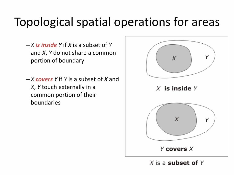
Topological spatial operations for areas–X is inside Y if X is a subset of Y
and X, Y do not share a common portion of boundary
–X covers Y if Y is a subset of X and X, Y touch externally in a common portion of their boundaries
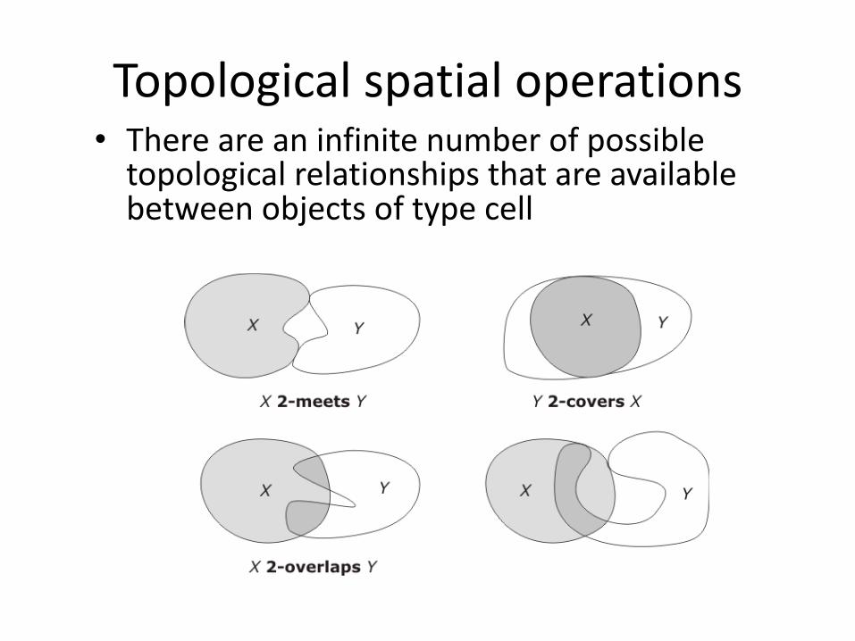
Topological spatial operations• There are an infinite number of possible
topological relationships that are available between objects of type cell

http://resources.esri.com/help/9.3/ArcGISDesktop/com/Gp_ToolRef/Data_Management_toolbox/select_by_location_colon_graphical_examples.htm

• Contain vs CONTAINS_CLEMENTINI: – the results of CONTAINS_CLEMENTINI will be
identical to CONTAINS with the exception that if the feature in the Selecting Features layer is entirely on the boundary of the Input Feature Layer, with no part of the contained feature properly inside the feature in the Input Feature Layer, the input feature will not be selected.

• Graphical examples:– http://webhelp.esri.com/arcgisdesktop/9.3/index.
cfm?topicname=select_by_location:graphical_examples

Spaghetti
• Spaghetti data structure represents a planar configuration of points, arcs, and areas
• Geometry is represented as a set of lists of straight-line segments

Spaghetti- example
• Each polygonal area is represented by its boundary loop
• Each loop is discretized as a closed polyline• Each polyline is represented as a list of points
A:[1,2,3,4,21,22,23,26,27,28,20,19,18,17]B:[4,5,6,7,8,25,24,23,22,21]C:[8,9,10,11,12,13,29,28,27,26,23,24,25]D:[17,18,19,20,28,29,13,14,15,16]
Issues
• There is NO explicit representation of the topological interrelationships of the configuration, such as adjacency
• Data consistence issues– Silver polygons– Data redundancy
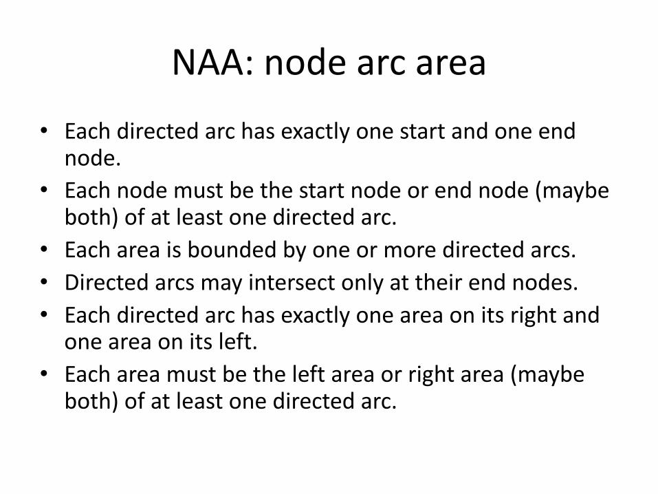
NAA: node arc area• Each directed arc has exactly one start and one end
node.• Each node must be the start node or end node (maybe
both) of at least one directed arc.• Each area is bounded by one or more directed arcs.• Directed arcs may intersect only at their end nodes.• Each directed arc has exactly one area on its right and
one area on its left.• Each area must be the left area or right area (maybe
both) of at least one directed arc.
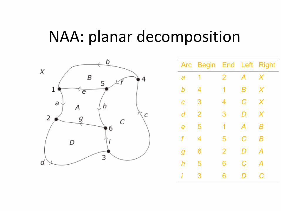
NAA: planar decompositionArc Begin End Left Right
a 1 2 A X
b 4 1 B X
c 3 4 C X
d 2 3 D X
e 5 1 A B
f 4 5 C B
g 6 2 D A
h 5 6 C A
i 3 6 D C

Field-based Approach
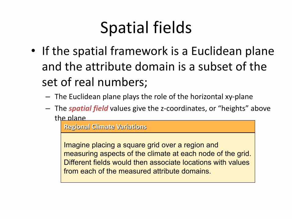
Spatial fields• If the spatial framework is a Euclidean plane
and the attribute domain is a subset of the set of real numbers;– The Euclidean plane plays the role of the horizontal xy-plane– The spatial field values give the z-coordinates, or “heights” above
the plane
Imagine placing a square grid over a region and measuring aspects of the climate at each node of the grid. Different fields would then associate locations with values from each of the measured attribute domains.
Regional Climate Variations

Properties of the attribute domain• The attribute domain may contain values which are
commonly classified into four levels of measurement– Nominal attribute: simple labels; qualitative; cannot be
ordered; and arithmetic operators are not permissible – Ordinal attribute: ordered labels; qualitative; and cannot be
subjected to arithmetic operators, apart from ordering– Interval attributes: quantities on a scale without any fixed
point; can be compared for size, with the magnitude of the difference being meaningful; the ratio of two interval attributes values is not meaningful
– Ratio attributes: quantities on a scale with respect to a fixed point; can support a wide range of arithmetical operations, including addition, subtraction, multiplication, and division
Continuous and differentiable fields
• Continuous field: small changes in location leads to small changes in the corresponding attribute value
• Differentiable field: rate of change (slope) is defined everywhere
• Spatial framework and attribute domain must be continuous for both these types of fields
• Every differentiable field must also be continuous, but not every continuous field is differentiable

One dimensional examples• Fields may be plotted as a graph of attribute
value against spatial framework
Continuous and differentiable; the slope of the curve can be defined at every point

One dimensional examplesThe field is continuous (the graph is connected) but not
everywhere differentiable. There is an ambiguity in the slope, with two choices at the articulation point between the two
straight line segments.
Continuous and not differentiable; the slope of the curve cannot be defined at one or more points

One dimensional examplesThe graph is not connected and so the field in not continuous
and not differentiable.
Not continuous and not differentiable

Two dimensional examples
• The slope is dependent on the particular location and on the bearing at that location
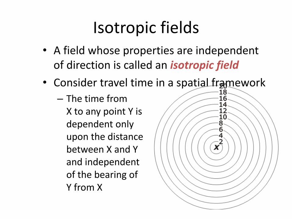
Isotropic fields• A field whose properties are independent
of direction is called an isotropic field• Consider travel time in a spatial framework– The time from
X to any point Y is dependent only upon the distance between X and Y and independent of the bearing of Y from X

Anisotropic fields• A field whose properties are dependent on
direction is called an anisotropic field.• Suppose there is a high speed link AB– For points near B it would be better, if traveling fromX, to travel to A, take the link,and continue on from B to the destination
– The direction to the destination is important
Representations of Spatial Fields
• Points• Contours• Raster/Lattice• Triangulation (Delaunay Triangulation)
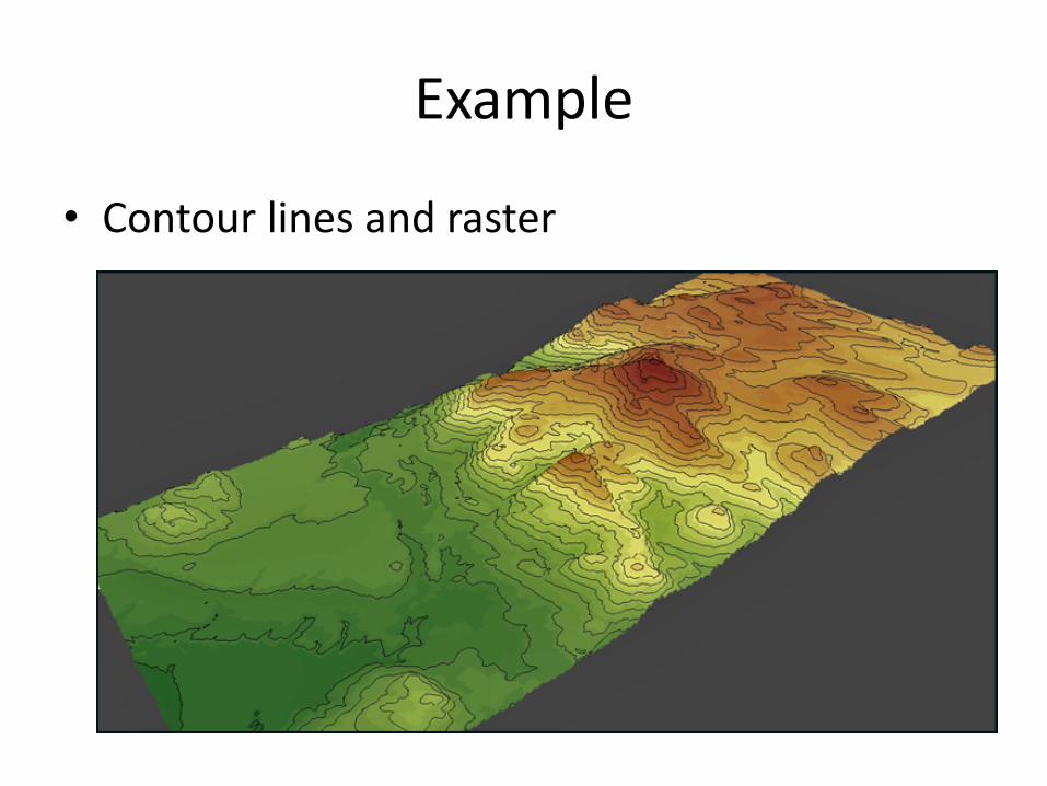
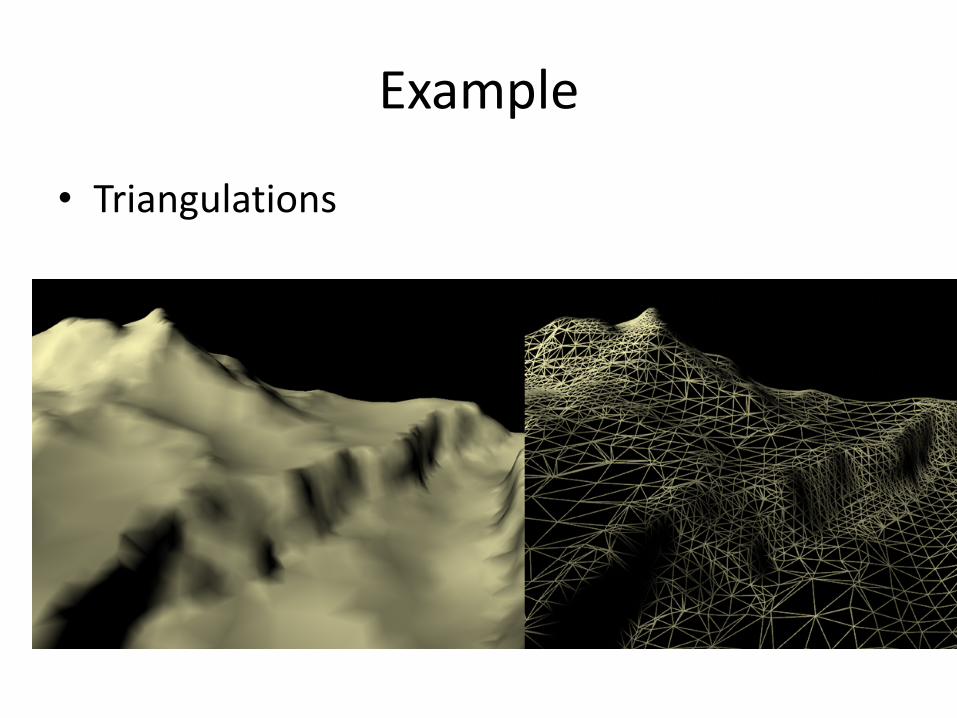
Example
• Contour lines and raster
Example
• Triangulations
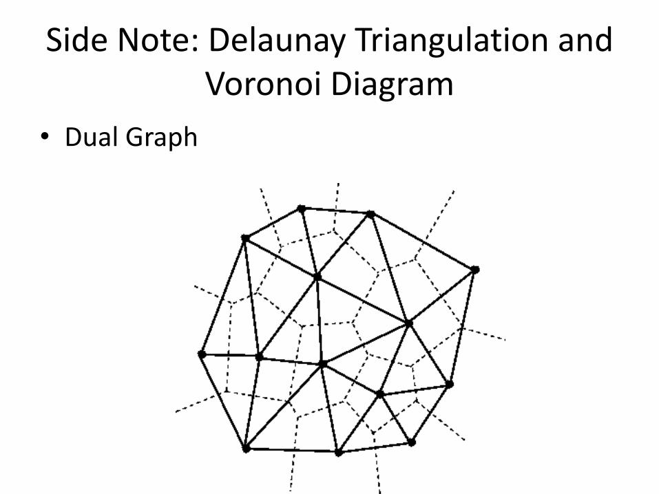
Side Note: Delaunay Triangulation and Voronoi Diagram
• Dual Graph

Operations on fields
• A field operation takes as input one or more fields and returns a resultant field
• The system of possible operations on fields in a field-based model is referred to as map algebra
• Three main classes of operations– Local– Focal– Zonal
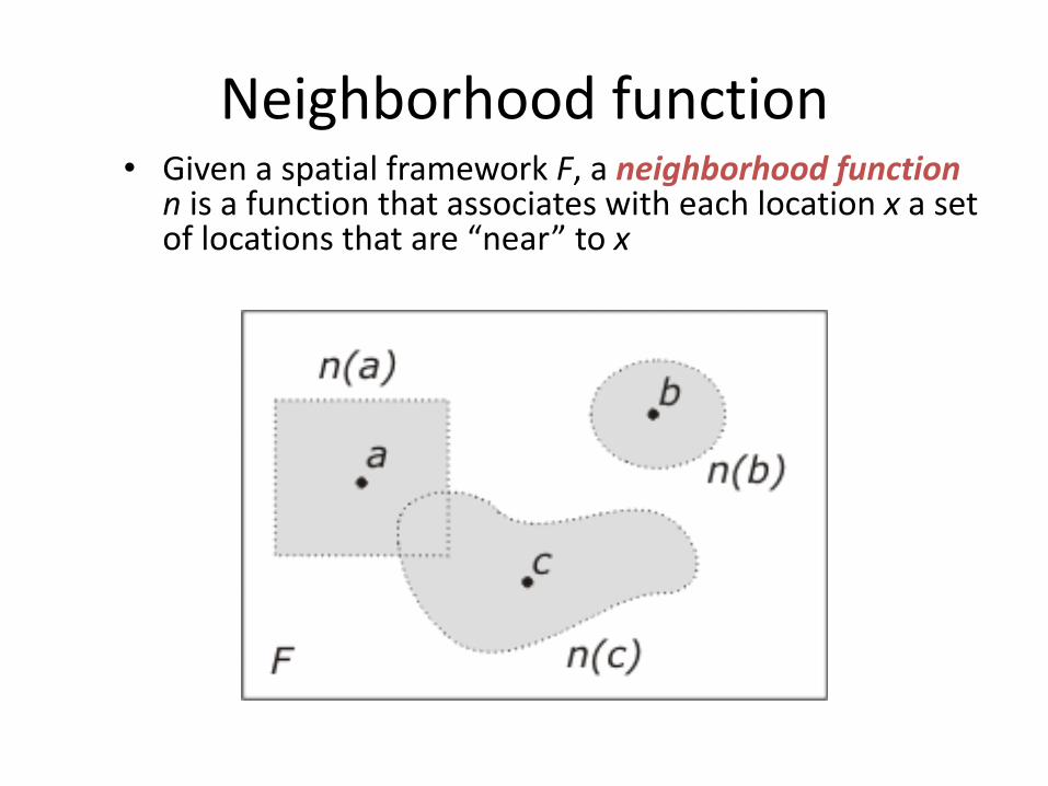
Neighborhood function• Given a spatial framework F, a neighborhood function
n is a function that associates with each location x a set of locations that are “near” to x

Local operations• Local operation: acts
upon one or more spatial fields to produce a new field
• The value of the new field at any location is dependent on the values of the input field function at that location● is any binary operation
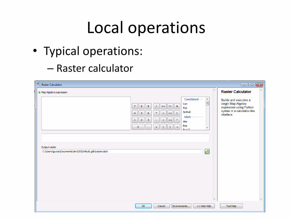
Local operations• Typical operations:– Raster calculator
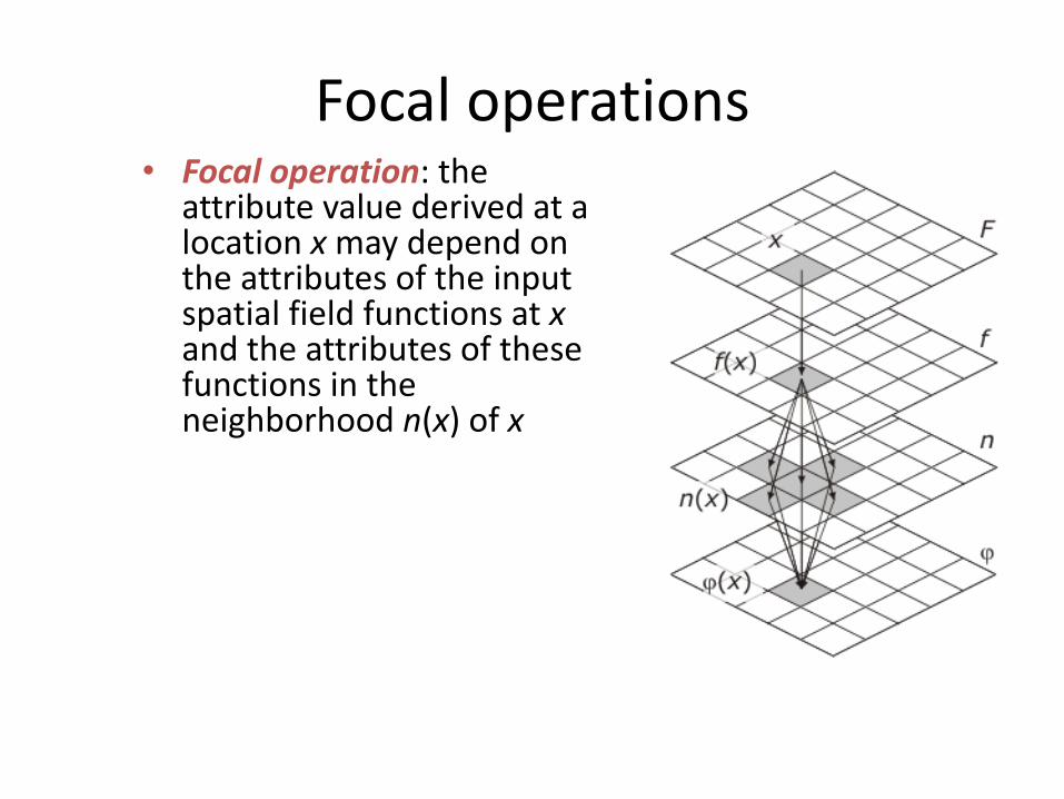
Focal operations• Focal operation: the
attribute value derived at a location x may depend on the attributes of the input spatial field functions at xand the attributes of these functions in the neighborhood n(x) of x
Focal operations• Typical operations:– Slope– Aspect– Hill shade– Focal statistics

Zonal operations• Zonal operation: aggregates
values of a field over a set of zones (arising in general from another field function) in the spatial framework
• For each location x:11 Find the Zone Zi in which x
is contained22 Compute the values of the
field function f applied to each point in Zi
3 Derive a single value ζ(x) of the new field from the values computed in step 2

Zonal operations• Typical operations:– Zonal – Viewshed– Watershed
More on Watershed Analysis

The terrain flow information model for deriving channels, watersheds, and flow related terrain
information. Raw DEM Pit Removal (Filling)
Flow FieldChannels, Watersheds, Flow Related Terrain Information
Watersheds are the most basic hydrologic landscape elements
Courtesy of Dr. David G. Tarboton

The Pit Removal Problem
• DEM creation results in artificial pits in the landscape
• A pit is a set of one or more cells which has no downstream cells around it
• Unless these pits are removed they become sinks and isolate portions of the watershed
• Pit removal is first thing done with a DEM
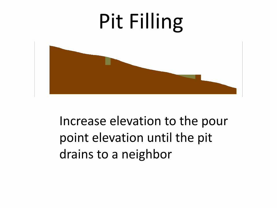
Increase elevation to the pour point elevation until the pit drains to a neighbor
Pit Filling
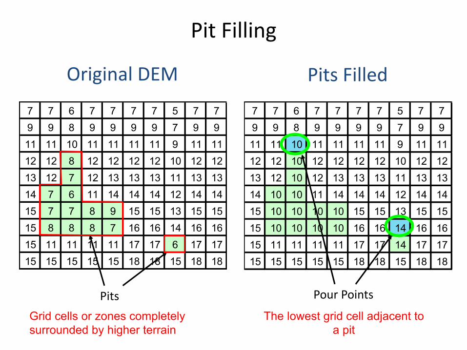
7 7 6 7 7 7 7 5 7 79 9 8 9 9 9 9 7 9 911 11 10 11 11 11 11 9 11 1112 12 10 12 12 12 12 10 12 1213 12 10 12 13 13 13 11 13 1314 10 10 11 14 14 14 12 14 1415 10 10 10 10 15 15 13 15 1515 10 10 10 10 16 16 14 16 1615 11 11 11 11 17 17 14 17 1715 15 15 15 15 18 18 15 18 18
Pit Filling
7 7 6 7 7 7 7 5 7 79 9 8 9 9 9 9 7 9 911 11 10 11 11 11 11 9 11 1112 12 8 12 12 12 12 10 12 1213 12 7 12 13 13 13 11 13 1314 7 6 11 14 14 14 12 14 1415 7 7 8 9 15 15 13 15 1515 8 8 8 7 16 16 14 16 1615 11 11 11 11 17 17 6 17 1715 15 15 15 15 18 18 15 18 18
Pits Pour Points
Original DEM Pits Filled
Grid cells or zones completely surrounded by higher terrain
The lowest grid cell adjacent to a pit

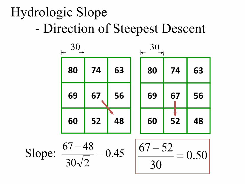
80 74 63
69 67 56
60 52 48
80 74 63
69 67 56
60 52 48
30
45.02304867
=-
50.0305267
=-Slope:
Hydrologic Slope - Direction of Steepest Descent
30
2 2 4 4 8
1 4 16
1 2 4 8 4
4 1 2 4 8
2 4 4 4 4
21
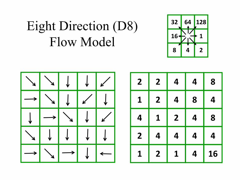
Eight Direction (D8) Flow Model
32
16
8
64
4
128
1
2
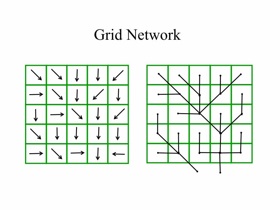
Grid Network

0 0 000
0
0
1
0
0
0
0
0
02 2 2
10 1
0 144 1
19 1
0 0 00 0
0
0
1
0
0
0
0
0
0
2 2 2
10 1
0
14
14
191
Flow Accumulation Grid. Area draining in to a grid cell
Link to Grid calculator
ArcHydro Page 72
0 0 00 0
0
0
1
0
0
0
0
0
0
2 2 2
10 1
0
14
14
191
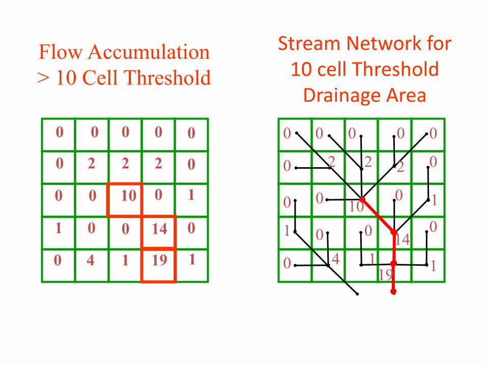
Flow Accumulation > 10 Cell Threshold
0 0 000
0
0
1
0
0
0
0
0
02 2 2
1
0
4 1 1
10
14
19
Stream Network for 10 cell Threshold
Drainage Area
1 1 11 1
1
1
2
1
1
1
1
1
1
3 3 3
11 2
1
25
15
202
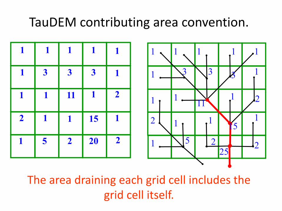
The area draining each grid cell includes the grid cell itself.
1 1 111
1
1
2
1
1
1
1
1
13 3 3
11 2
1
5 2225
15
TauDEM contributing area convention.

Watershed Draining to Outlet
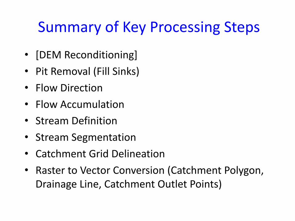
Summary of Key Processing Steps
• [DEM Reconditioning]• Pit Removal (Fill Sinks)• Flow Direction• Flow Accumulation• Stream Definition• Stream Segmentation• Catchment Grid Delineation• Raster to Vector Conversion (Catchment Polygon,
Drainage Line, Catchment Outlet Points)
Summary Concepts• The eight direction pour point model
approximates the surface flow using eight discrete grid directions
• The elevation surface represented by a grid digital elevation model is used to derive surfaces representing other hydrologic variables of interest such as– Slope– Flow direction– Drainage area– Catchments, watersheds and channel networks
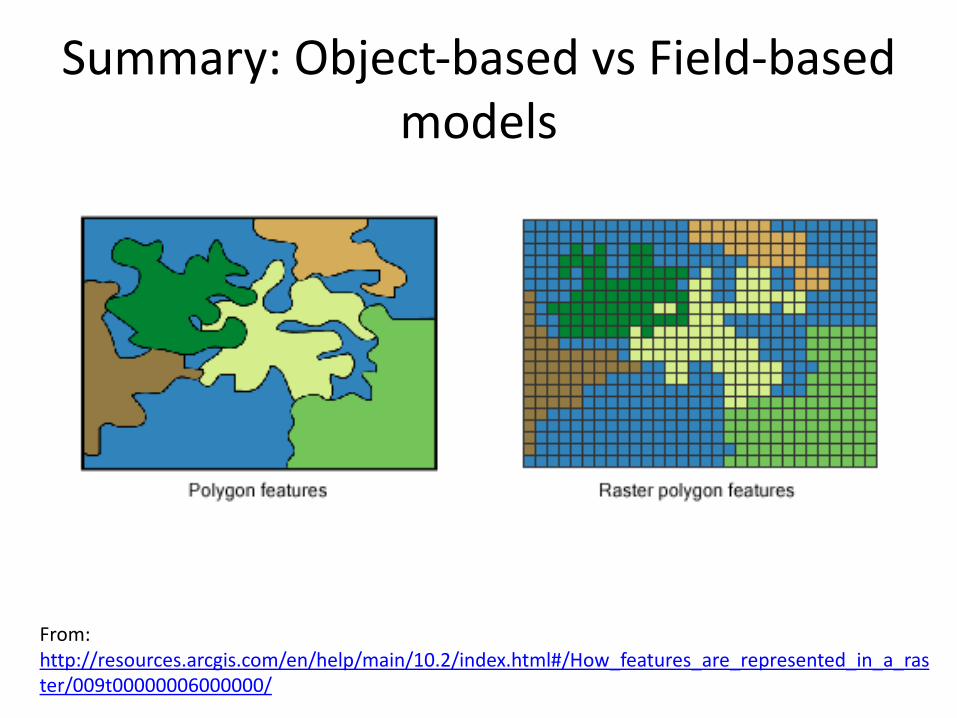
Summary: Object-based vs Field-based models
From: http://resources.arcgis.com/en/help/main/10.2/index.html#/How_features_are_represented_in_a_raster/009t00000006000000/
Summary: Object-based vs Field-based models
• Object-based models:– Greater precision– Less redundant information (smaller storage
footprints)– Complex data structures
• Field-based models:– Simpler data structures– More redundant information (larger storage
footprints)– Less precision
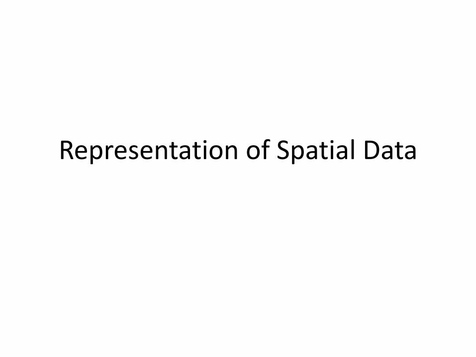
• Raster is faster, but vector is corrector
Raster <-> Vector
•Vector-> Raster–Interpolation•Inverse distance weighted, Kriging, Spline
–Density surface•Kernel density
–Rasterization•Raster->Vector–Watershed –Vectorization (raster to polygon)–…
Model Builder

Model Builder• Model Builder is a drag-and-drop interface to ArcToolbox
called ModelBuilder allowing you to develop a flow chart of your GIS workflow
• This flowchart is then run step by step to perform your analysis
• ArcGIS allows for custom scripting that can be added to ArcToolbox, introducing greater functionality
• Custom export scripts, specialized versions of existing tools, develop tools not available in ArcToolbox
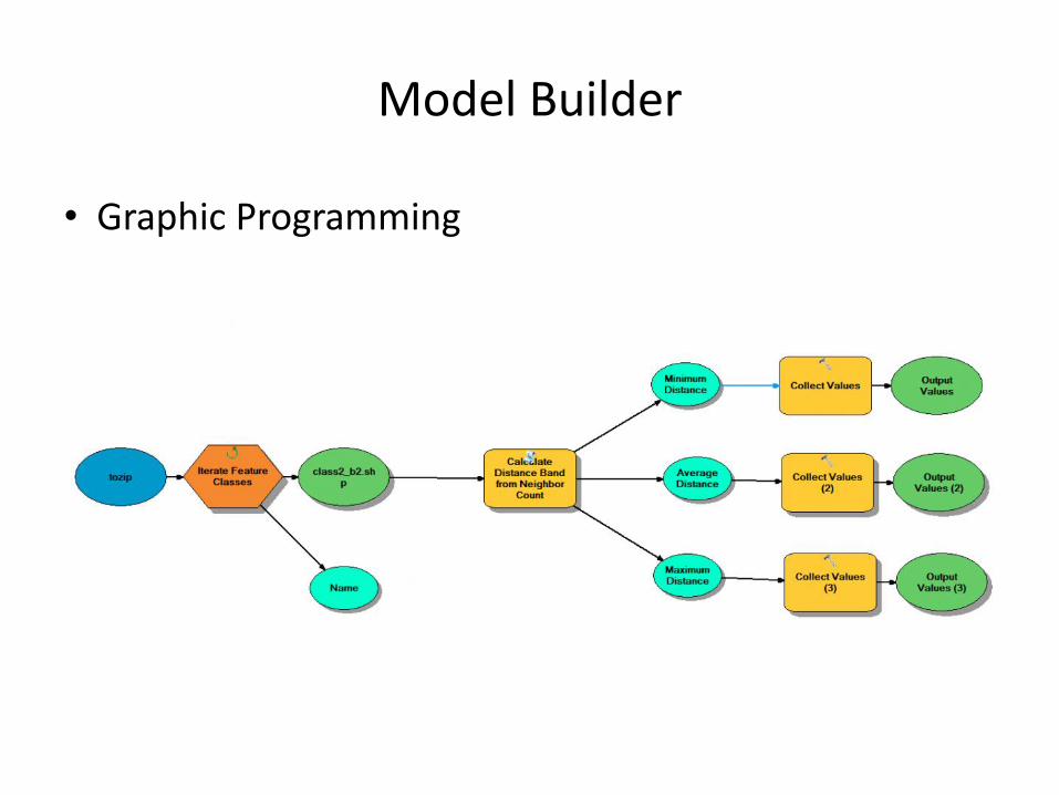
Model Builder
• Graphic Programming
Why Model Builder?• Developing a model for a GIS analysis allows for
repeat testing of a hypothesis using different data.
• The model can be coded into a GIS application, so that the steps are performed automatically.
• Easier reproduction of results.• Simplification of workflow.• Informs the computer how to conduct a series of
steps that would be impractical for you to do manually.

Reproducibility
• In performing an analysis, you must have your workflow clearly defined.
• This ensures that you are performing the steps in the correct order using the appropriate tools.
• Missteps are easy, especially when there can be hours of computer processing between steps.
• The GIS model can be exported as a graphic flowchart or a modeling data structure.

Workflow Efficiency
• There are many repetitive steps you will take in your daily workflow.
• Streamlining the process saves you time.• If you always start working in a File
Geodatabase with specific resolution and projection information, a model for generating your specialized GDB can be created.
Human Inefficiency
• You physically cannot perform the steps as fast as GIS can produce the results.
• Certain steps, such as iteration through a feature set would be prohibitively time consuming.
• Minimize the amount of time spent �babysitting� GIS to perform complex analyses.

Inside ArcToolbox

Demo• Demo• Lab: Buffalo commons using Model Builder: