Embed Size (px)
Citation preview

1
Sparse Representations in Audio and Music:from Coding to Source Separation
M. D. Plumbley, Member, IEEE, T. Blumensath, Member, IEEE, L. Daudet, Member, IEEE,R. Gribonval, Senior Member, IEEE, and M. E. Davies, Member, IEEE
Abstract—Sparse representations have proved a powerful toolin the analysis and processing of audio signals and already lieat the heart of popular coding standards such as MP3 andDolby AAC. In this paper we give an overview of a numberof current and emerging applications of sparse representationsin areas from audio coding, audio enhancement and musictranscription to blind source separation solutions that can solvethe “cocktail party problem”. In each case we will show how theprior assumption that the audio signals are approximately sparsein some time-frequency representation allows us to address theassociated signal processing task.
I. INTRODUCTION
Over recent years there has been growing interest in findingways to transform signals into sparse representations, i.e.representations where most coefficients are zero. These sparserepresentations are proving to be a particularly interesting andpowerful tool for analysis and processing of audio signals.
Audio signals are typically generated either by resonantsystems or by physical impacts, or both. Resonant systemsproduce sounds that are dominated by a small number offrequency components, allowing a sparse representation of thesignal in the frequency domain. Impacts produce sounds thatare concentrated in time, allowing a sparse representation ofthe signal in either directly the time domain, or in terms of asmall number of wavelets. The use of sparse representationstherefore appears to be a very appropriate approach for audio.
Manuscript received January XX, 200X; revised January XX, 200X. Thiswork was supported in part by the EU Framework 7 FET-Open project FP7-ICT-225913-SMALL: Sparse Models, Algorithms and Learning for Large-Scale data
M. D. Plumbley is with Queen Mary University of London, Schoolof Electronic Engineering and Computer Science, Mile End Road, LondonE1 4NS, UK (e-mail: [email protected]). He is supported bya Leadership Fellowship from the UK Engineering and Physical SciencesResearch Council (EPSRC).
T. Blumensath is with the School of Mathematics, University of Southamp-ton, Southampton, SO17 1BJ, UK (e-mail: [email protected]).
L. Daudet was at the time of writing with LAM, Institut Jean Le RonddAlembert, Universite Pierre et Marie Curie (UPMC Univ. Paris 06), 11 rue deLourmel, 75015 Paris, France (e-mail: [email protected]). In September2009 he joined the Langevin Institute for Waves and Images (LOA), UniversiteDenis DiderotParis 7.
R. Gribonval is with INRIA, Centre Inria Rennes—Bretagne Atlantique,Campus de Beaulieu, F-35042 Rennes Cedex, Rennes, France (e-mail:[email protected]).
M. E. Davies is with the Institute for Digital Communications (IDCOM) &Joint Research Institute for Signal and Image Processing, School of Engineer-ing and Electronics, University of Edinburgh, The King’s Buildings, MayfieldRoad, Edinburgh EH9 3JL, Scotland, UK (e-mail: [email protected]). Heacknowledges support of his position from the Scottish Funding Council andtheir support of the Joint Research Institute in Signal and Image Processingwith the Heriot-Watt University as a component part of the EdinburghResearch Partnership.
In this article, we will examine a range of applications ofsparse representations to audio and music signals. We willsee how this concept of sparsity can be used to design newmethods for audio coding which have improved performanceover non-sparse methods; how it can be used to performdenoising and enhancement on degraded audio signals; andhow it can be used to separate source signals from mixedaudio signals, particularly when there are more sources thanmicrophones. Finally, we will also see how finding a sparsedecomposition can lead to a note-like representation of musicalsignals, similar to automatic music transcription.
A. Sparse Representations of an Audio Signal
Suppose we have a sampled audio signal with T samplesx(t), 1 ≤ t ≤ T , which we can write in a row vector formas x = (x(1), . . . , x(T )). For audio signals we are typicallydealing with signals sampled below 20 kHz, but for simplicitywe will assume our sampled time t takes integer values. It isoften convenient to decompose x into a weighted sum of Qbasis vectors �q = (�q(1), . . . , �q(T )), with the contributionof the q-th basis vector weighted by a coefficient uq:
x(t) =
Q∑q=1
uq�q(t) or x =
Q∑q=1
uq�q (1)
or in matrix formx = uΦ (2)
where Φ is the matrix with elements [Φ]qt = �q(t).The most familiar representation of this type in audio signal
processing is the (Discrete) Fourier representation. Here wehave the same number of basis vectors as signal samples (Q =T ), and the basis matrix elements are given by
�q(t) =1
Texp
(2�j
Tqt
)(3)
where j =√−1. Now it remains for us to find the coefficients
uq in this representation of x. In the case of our Fourierrepresentation, this is straightforward: the matrix Φ is squareand invertible, and in fact orthogonal, so u can be calculateddirectly as u = xΦ−1 = x(TΦH), where the superscript ⋅Hdenotes the conjugate transpose.
Signal representations corresponding to invertible trans-forms such as the DFT, the discrete cosine transform (DCT),or the discrete wavelets transform (DWT) are convenient andeasy to calculate. However, it is possible to find many alterna-tive representations. In particular, if we allow the number of

2
basis vectors (and hence coefficients) to exceed the number ofsignal samples, Q > T , then solving (2) for the representationcoefficient vector u is in general not unique: there will be awhole (Q− T )-dimensional subspace of vectors u which sat-isfy x = uΦ. In this case we say that (2) is underdetermined.A common choice in this situation is to use the Moore-Penrosepseudoinverse Φ†, yielding u = xΦ†. However, in this articlewe are interested in finding representations that are sparse, i.e.representations where only a small number of the coefficientsof u are non-zero.
B. Advantages of sparse representations
Finding a sparse representation for a signal has manyadvantages for applications such as coding, enhancement,or source separation. In coding, a sparse representation hasonly a few non-zero values, so only these values (and theirlocations) need to be encoded to transmit or store the signal. Inenhancement, the noise or other disturbing signal is typicallynot represented by the same coefficients as the sparse signal.Therefore discarding the “wrong” coefficients can remove alarge proportion of the unwanted noise, leaving a much cleanerrestored signal. Finally, in source separation, if each signal tobe separated has a sparse representation, then there is a goodchance that there will be little overlap between the small setsof coefficients used to represent the different source signals.Therefore by selecting the coefficients “used” by each sourcesignal, we can restore each of the original signals with mostof the interference from the unwanted signals removed.
For typical steady-state audio signals, the Fourier repre-sentation already does quite a good job of providing anapproximately sparse representation. If an audio signal consistsof only stationary oscillations, without onsets or transients, arepresentation based on a short-time Fourier transform (STFT)or a Modified Discrete Cosine Transform (MDCT) [1] willinclude some large-amplitude coefficients corresponding to themain frequencies of oscillation of the signal, with little energyin between these.
However, audio signals also typically contain short tran-sients at the onsets of musical notes or other sounds. Thesewould not have a sparse representation in an STFT or MDCTbasis, but instead in such a representation would require a largenumber of frequency components to be active simultaneously.
One approach to overcome this is therefore to look for arepresentation in terms of a union of bases, each with differenttime-frequency characteristics. For example, we could createa “tall, thin” basis matrix
Φ =
[ΦC
ΦW
](4)
composed of both an MDCT basis ΦC, designed to representthe steady-state sinusoidal parts, and a Wavelet basis ΦW
designed to represent the transient, edge-like parts. We couldwrite this representation as
x = uΦ = uCΦC + uWΦW (5)
where the joint coefficient vector u = (uC uW) is a concatena-tion of the MDCT and Wavelet coefficients. This type of idea
is known in audio processing as hybrid representations [2] andalso appears in image processing as multilayered representa-tions [3] or Morphological Component Analysis [4]. Manyother unions are possible, such as unions of MDCT baseswith differing time-frequency resolutions. While the numberof basis vectors, and hence the number of possible coefficients,is larger in a union of bases, we may find that the resultingrepresentation has fewer non-zero coefficients and is thereforesparser (Fig. 1).
(a) (b)
1 2 3 4 5
103
104
Time (seconds)F
requ
ency
(H
z)1 2 3 4 5
103
104
Time (seconds)
Fre
quen
cy (
Hz)
Fig. 1. Representations of an audio signal in (a) a single MDCT basis, and(b) a union of eight MDCT bases with different window sizes (“8*MDCT”).
C. Recovering sparse representations
To find a sparse representation when the system is underde-termined is not quite so straightforward as for the square andinvertible case. Finding the true sparsest representation
arg minu{∥u∥0 ∣ x = uΦ} (6)
where the 0-norm ∥u∥0 is the number of non-zero elementsof u, is an NP-hard problem, so would take us a very longtime to solve. However, it is possible to find an approximatesolution to this. One method is to use the so-called BasisPursuit relaxation, where instead of looking to solve (6) welook for a solution to the easier problem
arg minu{∥u∥1 ∣ x = uΦ} (7)
where the 1-norm ∥u∥1 =∑q ∣uq∣ is the sum of the absolute
values. Eqn. (7) is equivalent to a linear program (LP), andcan be solved by a range of general or specialist methods, seee.g. [5], [6], [7], [8], [9], [10], [11].
Another alternative is to use a greedy algorithm to findan approximation to (6). For example, the matching pursuits(MP) algorithm [12] and orthogonal matching pursuit (OMP)algorithm [13] are well-known examples of this type of greedyalgorithm. There are many more in the literature [14], [15],[16] and considerable recent work in the area of sparserepresentations has concentrated on theoretically optimal andpractically efficient methods to find solutions (or approximatesolutions) to (6) or (7). Nevertheless, MP is still used in
3
real-world problems since there are efficient implementationsavailable, such as the Matching Pursuit Toolkit (MPTK)1 [17].
II. CODING
Coding is arguably the most straightforward applicationof sparse representations. Indeed, reversibly transforming thesignal into a new domain where the information is con-centrated on a few terms is the main idea underlying datacompression. The transform coder is a classical technique usedin source coding [18]. When the transform is orthonormalit can be shown (under certain assumptions) that the gainachievable through transform coding is directly linked to thetransform’s ability to concentrate the energy of the signal ina small number of coefficients [19]. However, this problemis not as straightforward as it may seem, since there is nosingle fixed orthonormal basis where all audio signals havea sparse representation. Audio signals are in general quitediverse in nature: they mostly have a strong tonal part, but alsosome lower-energy components such as transients components(at note attacks) and wide-band noise that are nonethelessimportant in the perception of audio signals. These tonal,transient and noise components are optimally represented inbases with different respective requirements in terms of time-frequency localization.
We will consider two main approaches to handle this issue.The first approach is to find an adapted orthonormal basis, bestfitted to the local features of the signal. This is the techniqueemployed in most state-of-the-art commercial audio codecs,such as MPEG 2/4 Advanced Audio Codec (AAC). The secondapproach uses dictionary redundancy to accommodate thisvariety of features, leading to a sparser representation, butwhere each coefficient carries more information.
A. Coding in adapted orthogonal bases
For coding, using an orthonormal basis seems an obviouschoice. Orthonormal bases yield invertible transforms with noredundancy, so the number of coefficients in the transformdomain is equal to the number of samples. Many multimediasignals have compact representations in orthonormal bases: forexample, images are often well suited to wavelet represen-tations (EZW, JPEG200). Furthermore, several orthonormalschemes also have fast implementations due to the specialstructure of the basis, such as the FFT for implementing theDFT, or Mallat’s multiresolution algorithm for the DWT [19].
For audio signals, a natural choice for an orthonormaltransform might be to use one based on the STFT. However,for real signals the Balian-Low theorem tells us that therecannot be a real orthonormal transform based on local Fouriertransforms with nice regularities properties both in time andfrequency.
To overcome this we can use so-called Lapped OrthogonalTransforms, which exploit special aliasing cancellation prop-erties of the cosine transform, when the window obeys twoconditions on symmetry and energy-preservation. The discrete
1mptk.irisa.fr
version of these classes of transforms leads to the ModifiedDiscrete Cosine Transform (MDCT) [1], with atoms such as
�k,p(t) = ℎ(�)
√2
Lcos
[�
L
(� +
1 + L
2
)(k +
1
2
)](8)
with L the frame size, � = t− pL and window ℎ(�) definedfor � = 0, . . . , 2L − 1. Again, there are a number of fastimplementations of the MDCT based on the FFT. The MDCTis one key to success of the ubiquitous “MP3” (MPEG-1 layerIII) coding standard, and is now used in the majority of state-of-the-art coding standards, such as MPEG 2/4 AAC.
Using the simple MDCT as described above has severelimitations. Firstly, it is not shift-invariant: at very-low bitrates,this can lead to so-called “warbling artefacts”, or “birdies” (asthese distortions appear most notably at the higher end of thespectrum). Seondly, the time resolution is limited: for a typicalframe size of L = 1024 samples at a 44.1 kHz samplingfrequency, the resolution is 43 Hz and time resolution is 23ms. For some very transient signals, such as drums or attacksat note onsets, this value is quite large: this leads to whatare known as pre-echo artefacts where the quantization noise“leaks” within the whole window, before the actual burst ofenergy.
However, the MDCT offers an extra degree of freedom inthe choice of the window. This leads to the field of adaptive(orthogonal) transforms: when the encoding algorithm detectsthat the signal is transient in nature, it switches to a “smallwindow” type, whose size is typically 1/8-th of the longwindow. The transition from long windows to short windows(and vice-versa) is performed by asymmetric windows.
B. Coding in overcomplete bases
Using overcomplete bases for coding may at first seemcounter-intuitive, as the number of analysis coefficients is in-creased. However, we can take advantage of the extra degreesof freedom to increase the sparsity of the set of coefficients:the larger the dictionary, the sparser a solution can be expected.Only those coefficients which are deemed to be significant willbe transmitted and coded, i.e. x(t) ≃∑ ∈Γ u � (t), where Γis a small subset of indices. However, the size of the dictionarycannot be increased at will to increase sparsity, for tworeasons. Firstly, solving the inverse problem is computationallyintensive and very large dictionaries may lead to overly longcomputations. Secondly, not only must the values {u } ∈Γ betransmitted, but also the subset { ∣ ∈ Γ} of significantparameters must itself be specified.
In [20], the simultaneous use of M = 8 MDCT bases wasproposed and evaluated, where the scales (frame sizes) Lm goas powers of two Lm = L02m, m = 1 . . . 8, with windowlengths from 128 to 16384 samples (2.9 ms to 370 ms).The 8-times overcomplete dictionary is now Dm = {�mkp ∣0 ≤ p < Pm, 0 ≤ k < LM}. To reduce pre-echo, largewindows are removed from the dictionary near onsets. Finally,the significant coefficients {u } ∈Γ are quantized and encodedtogether with their parameters { ∣ ∈ Γ}. For the sake ofefficiency, the sparse decomposition is performed using theMatching Pursuit algorithm [12].

4
Formal listening tests have shown that this coder (named“8*MDCT”) outperforms MPEG-2 AAC at very low bitrates(around 24 kbps) for some simple sounds while being ofsimilar quality for complex, polyphonic sounds. At the highestbitrates (above 64 kbps), where a large number of transformcoefficients have to be encoded and transmitted, having toencode the extra scale parameter becomes a heavy penalty,and the overcomplete dictionary performs slightly worse thanthe (adapted) orthogonal basis, although transparency can stillbe obtained in both cases.
C. New trends
A further key advantage of using overcomplete representa-tions such as “8*MDCT” is that a large part of the informationis carried by the significant scale-frequency-time parameters{ = (m, k, p) ∣ ∈ Γ}, which provide directly interpretableinformation about the signal content. This can be usefulfor instance in audio indexing for data mining: if a largesound database is available in an encoded format, a largequantity of user-intuitive information can be easily inferredfrom the sparse representation, at a very low computationalcost. The “8*MDCT” representation was found to have similarperformance to the state-of-the-art in common Music Infor-mation Retrieval tasks (e.g. rhythm extraction, chord analysis,and genre classification) while MP3 and AAC codecs onlyperformed well in the rhythm extraction, due to poor frequencyresolution of those transforms for the other tasks [21].
Sparse overcomplete representations also offer a step to-wards the “Holy Grail” of audio coding: object coding [22].In this paradigm, any recording would be decomposed intoa number of elementary constituents such as notes, or in-struments’ melodic lines, that could be rearranged at willwithout perceivable loss in sound quality. Of course, this iffar out of reach for current technology if we make no furtherassumptions on the signal, as this would imply that we wereable to fully solve both the “hard” problems of polyphonictranscription and the underdetermined source separation prob-lem. However, some attempts in very restricted cases [23],[24] indicate that this may be the right approach towards“musically-intelligent” coding.
D. Application to denoising
Finding an efficient encoding of an audio signal based onsparse representations can also help us with audio denoising.Typically, while the desired part of the signal is well repre-sented by the sparse representation, noise is typically poorlyrepresented by the sparse representation. By transformingour signal to its sparse representation, discarding the smallercoefficients, and reconstructing the signal again we have asimple way to suppress a significant part of the signal noise.
Many improvements can be made over this simple model.If this is considered in a Bayesian framework, the task is toestimate the most probable original signal given the corruptedobservation. Such a Bayesian framework allows the inclusionof structural priors for musical audio objects that take intoaccount the ‘vertical’ frequency structure of transients andthe ‘horizontal’ structure of tonals, as well as the variance
of the residual noise. Such a structured model can help toreduce the so-called ‘birdies’ or ‘musical noise’ that can occurdue to switching of time-frequency coefficients. However,calculating the sparse representation is more complex thana straightforward Basis Pursuit method, but Markov chainMonte-Carlo (MCMC) methods have been used for this [25].
III. SOURCE SEPARATION
In many applications, audio recordings are mixtures ofunderlying audio signals and it is desirable to recover thoseoriginal signals. For example, in a meeting room we may haveseveral microphones, but each one collects a mixture of severaltalkers. To automatically transcribe the minutes of a meeting, afirst step would be to separate these into one channel per talker.Sparse representations can be of significant help in solving thistype of source separation problem.
Let us first consider the instantaneous mixing model, wherewe ignore time delays and reverberation. Here we have J audiosources sj(t), j = 1, . . . , J which are instantaneously mixedto give I observations xi(t), i = 1, . . . , I according to
xi(t) =
J∑j=1
aijsj(t) + ei(t) (9)
where aij is the amount of source j that appears in observationi, and ei(t) is noise on the observation xi(t). This type ofmixture might occur in, for example, pan-potted stereo, whereearly stereo recordings were produced by changing the amountof each source mixed to the left and right channels withoutany time delays or other effects2. We can also write (9) invector or matrix notation as
x(t) =∑j
ajsj(t) + e(t) or X = AS + E (10)
where e.g. the matrix X is an I×T matrix with columns x(t)and rows xi, and aj is the jth column of the mixing matrixA = [aij ].
If the noise E is small, the mixing matrix A is known, andA is square (I = J) and full rank, then we can estimate thesources using s(t) = A−1x(t); if we have more observationsthan sources (I > J) we can use the pseudo-inverse s(t) =A†x(t). If A is not known (blind source separation) then wecould use a technique such as independent component analysis(ICA) to estimate it [26].
However, if we have fewer observations than sources (I <J), then we cannot use matrix inversion (or pseudo-inversion)to unmix the sources. In this case, called underdeterminedsource separation [27], [28], we can use sparse representationsboth to help separate the sources, and, for blind sourceseparation, to estimate the mixing matrix A.
A. Underdetermined separation by binary masking
If we transform the signal mixtures xi = (xi(t))1≤t≤T intoa domain where they have a sparse representation, it is likelythat most coefficients of the transformed mixture correspond to
2A more accurate model for acoustic recordings is the convolutive modelconsidered below in Eq. (16)

5
either none or only one of the original sources. By identifyingand matching up the sources present in each coefficient, wecan recover the original, unmixed sources. Suppose that our Jsource signals sj all have sparse representations using atoms�q from a full rank Q×T basis matrix Φ (with Q = T ), i.e.,
sj =∑q
zjq�q 1 ≤ j ≤ J (11)
where zjq are the sparse representation coeffients. In matrixnotation we can write S = ZΦ and Z = SΦ−1.
Now denoting U = XΦ−1 the representation of X in thebasis Φ, for noiseless instantaneous mixing we have
U = AZ. (12)
For a simple special case, suppose that Z is so sparse that atmost one source coefficient jq is active at each transform indexq, i.e. zjq = 0 for j ∕= jq . In other words, each column of Zcontains at most one nonzero entry, and the source transformedrepresentations are said to have disjoint supports. Then (12)becomes
uq = ajqzjq,q 1 ≤ q ≤ Q (13)
so that each vector uq is a scaled version of one of the mixingmatrix columns aj . Therefore, when A is known, for each qwe can estimate jq by finding the mixing matrix column ajwhich is most correlated with uq:
jq = arg maxj
∣aTj uq∣∥aj∥2
1 ≤ q ≤ Q (14)
and we construct a mask "jq = 1 if j = jq , 0 otherwise.Therefore using this mask to identify the active sources, andmultiplying (13) by aT
jqand rearranging we get
zjq = "jqaTj uq
∥aj∥2(15)
from which we can estimate the sources as S = ZΦ. Dueto the binary nature of "jq this approach is known as binarymasking.
Even though the assumption that the sources have disjointsupports in the transformed domain is not satisfied for mostreal audio signals and standard transforms, the binary maskingapproach remains relevant to obtain accurate (although nonexact) estimates of the sources as soon as they have almostdisjoint supports, i.e., at each transform index q at most onesource j has a non negligible coefficient zjq .
The assumption that the sources have essentially disjointsupports in the transformed domain is highly dependent onthe chosen transform matrix Φ. This is illustrated in Fig. 2where on top we displayed the coefficients zj of three musicalsources (i.e. J = 3) in some domain Φ, below we displayedthe coefficients ui ∈ ℝ2 of a stereophonic mixture of thesources (i.e., I = 2) in the same domain, and at the bottomwe displayed the scatter plot of uq , that is to say the collectionof {uq, 1 ≤ q ≤ Q} .
On the left (Fig. 2-(a)), the three musical sources are playingone after another, and the transform is simply the identitymatrix Φ = I, which is associated with the so-called Dirac
basis. At each time instant t, a single source is active, hencethe scatter plot of uq clearly displays “spokes”, with directionsgiven by the columns aj of A. In this simple case, the sourcescan be separated by simply segmenting their time-domainrepresentation using (14) to determine which source is activeat each time instant.
In the middle (Fig. 2-(b)), the three musical sources areplaying together, and the transform is still the Dirac basisΦ = I. The disjoint support assumption is clearly violatedin the time domain, and the scatter plot no longer revealsthe directions of the columns aj of A. On the right (Fig. 2-(c)), the same three musical sources as in Fig. 2-(b) aredisplayed but in the time-frequency domain rather than thetime domain, using the MDCT transform, i.e., the atoms �q aregiven by (8). On the top we observe that, for each source, manytransform coefficients are small while only a few of them arenon negligible and appear as spikes. A detailed study wouldshow that these spikes appear at different transform indices qfor different sources, so for each transform index there is atmost one source coefficient j which is non negligible. Thisis confirmed by the scatter plot at the bottom, where we cansee that the vectors uq are concentrated along “spokes” in thedirections of the columns aj of A.
As well as allowing separation for known A, the scatterplot at the bottom of Fig. 2-(c) also illustrates that sparserepresentations also allow us to estimate A from the data,in the blind source separation case. If at most one sourcecoefficient is active at each transform index q, then thedirections of the “spokes” in Fig. 2-(c) correspond to thecolumns of A. Therefore estimation of the columns aj of A,up to a scaling ambiguity, becomes a clustering problem whichcan be addressed using e.g. K-means or weighted variants [27],[29], [30], [31].
Finally, we mention that binary masking can also be usedwhen only one channel is available, provided that at most onesource is significantly active at each time-frequency index.However in the single channel case we no longer have adirection aj to allow us to determine which source is activeon which transform index q. Additional statistical informationmust be exploited to identify the active sources and build theseparating masks "jq ∈ {0, 1}. For example, non-negative ma-trix factorization (NMF) or Gaussian Mixture Models (GMMs)of short time Fourier spectra can be used to build non-binaryversions of these masks 0 ≤ "jq ≤ 1, associated with time-varying Wiener filtering [32], [33], [34].
B. Time-frequency masking of anechoic mixtures
Binary masking can also be extended when there is noise,and when the mixture process is convolutive, rather thaninstantaneous. The convolutive mixing model, which accountsfor the sound relections on the walls of a meeting room andthe overall reverberation, is as follows:
xi(t) ≈J∑j=1
+∞∑n=−∞
aij(n)sj(t− n), 1 ≤ i ≤ I, (16)
where aij(n) is the mixing filter applied to source j to getits contribution to observation i. In matrix notation we can

6
0 0.2 0.4 0.6 0.8 1 1.2 1.4 1.6 1.8 2
x 105
−1
0
1
(a) Sources disjoint in time
t
s 1(t)
0 0.2 0.4 0.6 0.8 1 1.2 1.4 1.6 1.8 2
x 105
−0.5
0
0.5
ts 2(t
)
0 0.2 0.4 0.6 0.8 1 1.2 1.4 1.6 1.8 2
x 105
−0.5
0
0.5
t
s 3(t)
0 0.2 0.4 0.6 0.8 1 1.2 1.4 1.6 1.8 2
x 105
−1
0
1
(b) Musical sources
t
s 1(t)
0 0.2 0.4 0.6 0.8 1 1.2 1.4 1.6 1.8 2
x 105
−0.5
0
0.5
t
s 2(t)
0 0.2 0.4 0.6 0.8 1 1.2 1.4 1.6 1.8 2
x 105
−0.5
0
0.5
t
s 3(t)
0 0.2 0.4 0.6 0.8 1 1.2 1.4 1.6 1.8 2
x 105
−20
0
20
(c) MDCT of sources
q
z 1q
0 0.2 0.4 0.6 0.8 1 1.2 1.4 1.6 1.8 2
x 105
−5
0
5
q
z 2q
0 0.2 0.4 0.6 0.8 1 1.2 1.4 1.6 1.8 2
x 105
−20
0
20
q
z 3q
0 0.2 0.4 0.6 0.8 1 1.2 1.4 1.6 1.8 2
x 105
−1
−0.5
0
0.5
1
Sources Mixture
t
x 1(t)
0 0.2 0.4 0.6 0.8 1 1.2 1.4 1.6 1.8 2
x 105
−0.5
0
0.5
t
x 2(t)
0 0.2 0.4 0.6 0.8 1 1.2 1.4 1.6 1.8 2
x 105
−1
−0.5
0
0.5
1
Sources Mixture
t
x 1(t)
0 0.2 0.4 0.6 0.8 1 1.2 1.4 1.6 1.8 2
x 105
−0.5
0
0.5
tx 2(t
)
0 0.2 0.4 0.6 0.8 1 1.2 1.4 1.6 1.8 2
x 105
−20
−10
0
10
20
MDCT of the sources mixture
q
u 1q
0 0.2 0.4 0.6 0.8 1 1.2 1.4 1.6 1.8 2
x 105
−20
−10
0
10
20
q
u 2q
−0.8 −0.6 −0.4 −0.2 0 0.2 0.4 0.6 0.8−0.8
−0.6
−0.4
−0.2
0
0.2
0.4
0.6
0.8
x1(t)
x 2(t)
Scatter plot
−0.8 −0.6 −0.4 −0.2 0 0.2 0.4 0.6 0.8−0.8
−0.6
−0.4
−0.2
0
0.2
0.4
0.6
0.8
x1(t)
x 2(t)
Scatter plot
−20 −15 −10 −5 0 5 10 15 20−20
−15
−10
−5
0
5
10
15
20
u1q
u 2q
Scatter plot
Fig. 2. Top: coefficients of three musical sources. Middle: coefficients of two mixtures of the three sources. Bottom: scatter plot of the mixture coefficients(plain lines indicate the directions aj of the columns of the mixing matrix, the colors indicate to which source is associated which column). Left (a): thethree musical sources do not play together; time domain coefficients. Middle (b): the three musical sources play together; time domain coefficients. Right (c):the three musical sources play together; time-frequency (MDCT) domain coefficients.
write X ≈ A ★ S, where ★ denotes convolution. The STFTof both sides yields an approximate time-frequency domainmixing model [27]
Xi(!, �) ≈J∑j=1
Aij(!)Sj(!, �), 1 ≤ i ≤ I. (17)
at frequency ! and time frame � . For anechoic mixtures, weignore reverberation but allow different propagation times andattenuations between each source and each microphone. Herethe mixing filters aij(n) become simple gains aij and delaysnij , giving Aij(!) = aij exp(2j�nij!).
At time-frequency index (!, �), suppose that we know thatthe only significant source coefficients are indexed by j ∈ J =J (!, �), i.e., Sj(!, �) ≈ 0 for j /∈ J . Then (17) becomes
Xi(!, �) ≈∑j∈J
Aij(!)Sj(!, �), 1 ≤ i ≤ I, (18)
so that the vectors u = u(!, �) := (Xi(!, �))Ii=1 and z =z(!, �) := (Sj(!, �))Jj=1 satisfy
u ≈ AJ (!)zJ (19)
where AJ (!) = (Aij(!))1≤i≤I,j∈J and zJ = (zj)j∈J .Therefore, for each time-frequency index (!, �), if we know
the matrix A(!) and the set J = J (!, �) of most significantly
active sources, we can estimate the source coefficients as [35]
[Sj(!, �)]j∈J := A†J (!)u(!, �) (20)
[Sj(!, �)]j /∈J := 0 (21)
where AJ (!) is the mixing filter submatrix for the activesources at frequency !. Each source can finally be recon-structed by inverse STFT, using e.g. the overlap-add method.
In practice, if we only know the matrix A(!), the criticaldifficulty is to identify the set J of most significantly activesources. For a “reasonably small” number of sources with“sufficiently sparse” time-frequency representations, straight-forward statistical considerations show that, at most time-frequency points (!, �), the total number of active sources issmall and does not exceed some J ′ ≤ I . Identifying the set Jof active source amounts to searching for an approximationu ≈ A(!)z where z has few nonzero entries. This is asparse approximation problem, which needs to be addressedindependently at each time-frequency point.
While binary masking corresponds to searching for z withat most one nonzero entry (J ′ = 1) [27], non-binary maskingcan be performed choosing, e.g., the minimum 1-norm z suchthat u = A(!)z (Basis Pursuit) (7), as proposed in [28], orthe minimum p-norm solution with p < 1 [36].
We have seen in this section that sparse representationscan be particularly useful when tackling source separationproblems. As well as the approaches we have touched on here

7
there are many other interesting methods, such as convolutiveblind source separation and sparse filter models, which involvesparse representations in the time and/or time-frequency do-mains. For surveys of some these methods see e.g. [37], [38].
IV. AUTOMATIC MUSIC TRANSCRIPTION
So far the coefficients in the sparse representation have beenfairly arbitrary, so we were only interested in whether such asparse representation exists, not specifically what the coeffi-cients mean. However, in some cases, we can assign a specificmeaning to the sparse coefficients themselves. For example, ina piece of keyboard music, such as a harpsichord or piano solo,only a few of the many possible notes are playing at any onetime. Therefore the notes form a sparse representation whencompared to, for example, a time-frequency spectrogram.
In the simplest case, suppose that x(�) =(X(1, �), . . . , X(!, �), . . . , X(K, �))T is the spectrumat frame � . Then we approximate this by the model
x(�) ≈ As(�) =∑q
aqSq(�) (22)
where aq is the contribution of the spectrum due to note q, ands(�) = (S1(�), . . . , SQ(�))T is the vector of note activitiesSq(�) at frame � . In this simple case, we are assuming thateach note q produces just a scaled version of the note spectraaq at each frame � .
Joining all these spectral vectors together across frames, inmatrix notation we get
X ≈ AS. (23)
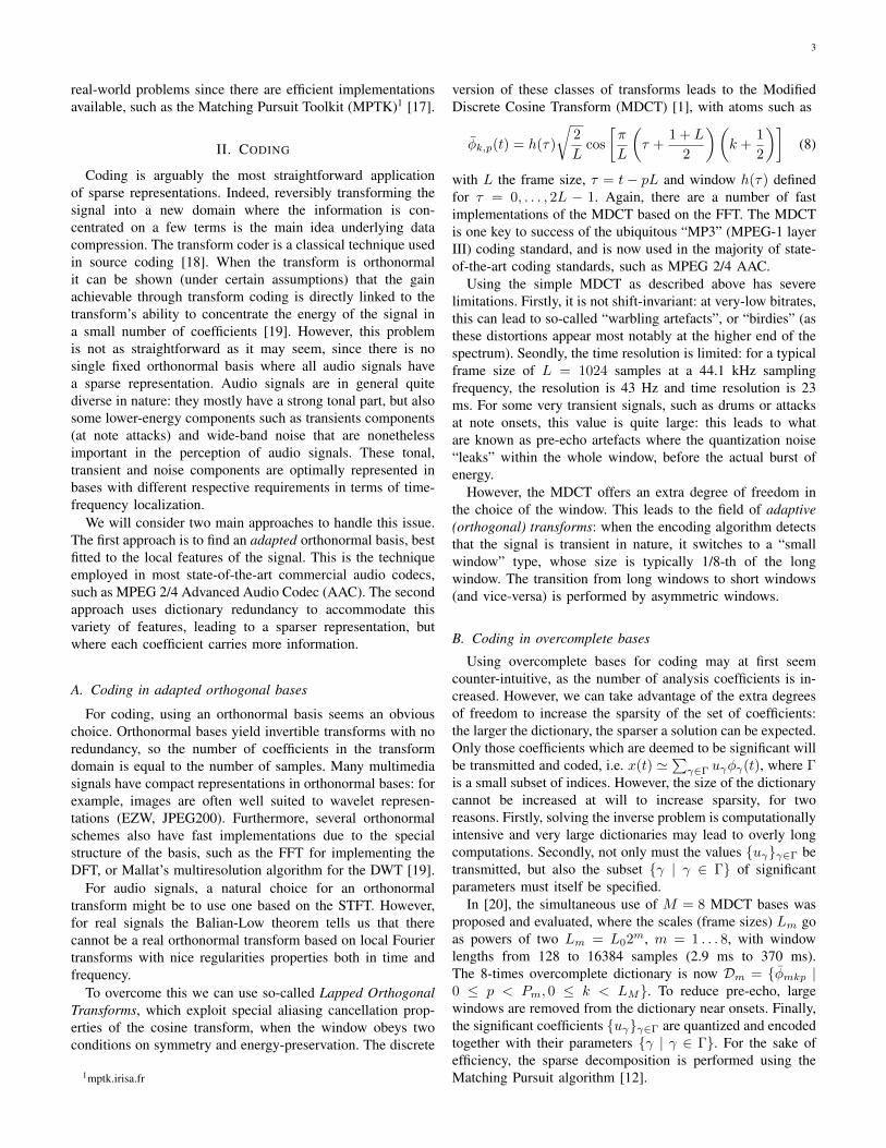
The basis dictionary A is no longer of a fixed MDCTor FFT form, but instead must be learned from the dataX = [x(�)]. To do this, we can use methods such as gradientdescent in a probabilistic framework [39], [40] or the recentK-SVD algorithm [41]. When applied to MIDI-synthesizedharpsichord music, this simple model is able to identify mostof the notes present in the piece, and produce a sparse ‘piano-roll’ representation of the music, a simple version of automaticmusic transcription (Fig. 3). For more complex sounds, suchas those produced by a real piano, the simple assumption ofscaled spectra per note no longer holds, and several sparsecoefficients are typically needed to represent each note [42].
It is also possible to apply this sparse representations modeldirectly in the time domain, by searching for shift-invariantsparse coding of the musical audio waveforms. Here a ‘spik-ing’ representation of the signal is found, which combines withthe shift-invariant dictionary to generate the audio signal. Formore details and a comparison of these methods, see [43].
V. CONCLUSIONS
In this article we have given an overview of a number ofcurrent and emerging applications of sparse representationsto audio signals. In pariticular, we have seen how we canuse sparse representations in audio coding, denoising, sourceseparation, and automatic music transcription. We believe thatis an exciting area of research, and we anticipate that therewill be many further advances in this area in the future.
ACKNOWLEDGEMENTS
The authors would like to thank Emmanuel Ravelli forFig. 1, Simon Arberet for Fig. 2 and Samer Abdallah for Fig. 3.
REFERENCES
[1] H. Malvar, “A modulated complex lapped transform and its applicationsto audioprocessing,” in Proc. Int. Conf. Acoust., Speech, and SignalProcess. (ICASSP’99), vol. 3, 1999.
[2] L. Daudet and B. Torresani, “Hybrid representations for audiophonicsignal encoding,” Signal Processing, special issue on Image and VideoCoding Beyond Standards, vol. 82, no. 11, pp. 1595–1617, 2002.
[3] F. Meyer, A. Averbuch, and R. Coifman, “Multilayered image represen-tation: Application to image compression,” IEEE Trans. Image Process.,vol. 11, no. 9, pp. 1072–1080, 2002.
[4] J.-L. Starck, M. Elad, and D. L. Donoho, “Redundant multiscale trans-forms and their application for Morphological Component Analysis,”Journal of Advances in Imaging and Electron Physics, vol. 132, pp.287–348, 2004.
[5] S. S. Chen, D. L. Donoho, and M. A. Saunders, “Atomic decompositionby basis pursuit,” SIAM Journal on Scientific Computing, vol. 20, pp.33–61, 1998.
[6] I. Daubechies, M. Defrise, and C. De Mol, “An iterative thresholdingalgorithm for linear inverse problems with a sparsity constraint,” Com-munications on Pure and Applied Mathematics, vol. 57, no. 11, pp.1413–1457, Aug. 2004.
[7] B. Efron, T. Hastie, I. Johnstone, and R. Tibshirani, “Least angleregression,” Annals of Statistics, vol. 32, no. 2, pp. 407–499, Apr. 2004.
[8] M. Figueiredo, J. Bioucas-Dias, and R. Nowak, “Majorization-minimization algorithms for wavelet-based image restoration,” IEEETrans. Image Process., vol. 16, no. 12, pp. 2980–2991, Dec. 2007.
[9] M. Elad, B. Matalon, and M. Zibulevsky, “Coordinate and subspaceoptimization methods for linear least squares with non-quadratic regu-larization,” Appl. Comput. Harm. Anal., vol. 23, pp. 346–367, 2007.
[10] W. Yin, S. Osher, D. Goldfarb, and J. Darbon, “Bregman iterative al-gorithms for l1-minimization with applications to compressed sensing,”SIAM J. Imaging Sciences, vol. 1, no. 1, pp. 143–168, 2008.
[11] P. L. Combettes and J.-C. Pesquet, “A proximal decomposition methodfor solving convex variational inverse problems,” Inverse Problems,vol. 24, article ID 065014 (27pp), 2008.
[12] S. Mallat and Z. Zhang, “Matching pursuits with time-frequency dictio-naries,” IEEE Trans. Signal Process., vol. 41, no. 12, pp. 3397–3415,1993.
[13] Y. C. Pati, R. Rezaiifar, and P. S. Krishnaprasad, “Orthogonal matchingpursuit: Recursive function approximation with applications to waveletdecomposition,” in Conference Record of The Twenty-Seventh AsilomarConference on Signals, Systems and Computers, Pacific Grove, CA, 1-3Nov. 1993, pp. 40–44.
[14] D. Needell and R. Vershynin, “Uniform uncertainty principle and signalrecovery via regularized orthogonal matching pursuit,” Foundations ofComputational Mathematics, vol. 9, pp. 317–334, 2009.
[15] D. Needell and J. Tropp, “CoSaMP: Iterative signal recovery fromincomplete and inaccurate samples.” Applied Computational HarmonicAnalysis, vol. 26, pp. 301–321, 2009.
[16] T. Blumensath and M. Davies, “Iterative hard thresholding for com-pressed sensing,” Applied and Computational Harmonic Analysis, 2009,in Press.
[17] S. Krstulovic and R. Gribonval, “MPTK: Matching Pursuit madetractable,” in Proc. Int. Conf. Acoust. Speech Signal Process.(ICASSP’06), vol. 3, Toulouse, France, May 2006, pp. III–496–499.
[18] A. Gersho and R. M. Gray, Vector quantization and signal compression.Boston: Kluwer, 1992.
[19] S. Mallat, A Wavelet Tour of Signal Processing: The Sparse Way, 3rd ed.Academic Press, 2009.
[20] E. Ravelli, G. Richard, and L. Daudet, “Union of MDCT bases foraudio coding,” IEEE Transactions on Audio, Speech, and LanguageProcessing, vol. 16, no. 8, pp. 1361–1372, Nov. 2008.
[21] ——, “Audio signal representations for indexing in the transform do-main,” IEEE Transactions on Audio, Speech, and Language Processing,vol. to appear, 2009.
[22] X. Amatriain and P. Herrera, “Transmitting audio content as soundobjects,” in Proceedings of the AES 22nd International Conference onVirtual, Synthetic and Entertainment Audio, Espoo, Finland, 2002.

8
X ≈ A × S
time/s
freq
uenc
y/kH
z
harpsichord input
0 1 2 3 4 5 6 70
1
2
3
4
5
freq
uenc
y/kH
z
harpsichord dictionary
10 20 30 40 500
1
2
3
4
5
com
pone
nt
time/s
harpsichord output
0 1 2 3 4 5 6 7
10
20
30
40
50
Fig. 3. Transcription of the music spectrogram X = [x(�)] into the individual note spectra A = [aq ] and note activitites S = [Sq(�)] [42].
[23] E. Vincent and M. D. Plumbley, “Low bitrate object coding of musicalaudio using Bayesian harmonic models,” IEEE Transactions on Audio,Speech, and Language Processing, vol. 15, no. 4, pp. 1273–1282, May2007.
[24] G. Cornuz, E. Ravelli, P. Leveau, and L. Daudet, “Object coding ofharmonic sounds using sparse and structured representations,” in Proc. ofthe 10th Int. Conference on Digital Audio Effects (DAFx-07), Bordeaux,2007, pp. 41–46.
[25] C. Fevotte, B. Torresani, L. Daudet, and S. J. Godsill, “Sparse linearregression with structured priors and application to denoising of musicalaudio,” IEEE Transactions on Audio, Speech and Language Processing,vol. 16, pp. 174–185, 2008.
[26] A. Hyvarinen, J. Karhunen, and E. Oja, Independent Component Anal-ysis. John Wiley & Sons, 2001.
[27] O. Yilmaz and S. Rickard, “Blind separation of speech mixtures viatime-frequency masking,” IEEE Transactions on Signal Processing,vol. 52, no. 7, pp. 1830–1847, Jul. 2004.
[28] P. Bofill and M. Zibulevsky, “Underdetermined blind source separationusing sparse representations,” Signal Processing, vol. 81, no. 11, pp.2353–2362, Nov. 2001.
[29] F. Abrard and Y. Deville, “Blind separation of dependent sources usingthe “TIme-Frequency Ratio Of Mixtures” approach,” in Proc. SeventhInternational Symposium on Signal Processing and Its Applications(ISSPA 2003), vol. 2, Paris, France, Jul. 2003, pp. 81–84.
[30] S. Arberet, R. Gribonval, and F. Bimbot, “A robust method to count andlocate audio sources in a stereophonic linear instantaneous mixture,”in Proc. 6th Intl. Conf. on Independent Component Analysis and BlindSignal Separation (ICA 2006), Charleston, SC, USA, ser. LNCS 3889,J. Rosca et al., Eds. Springer, Mar. 2006, pp. 536–543.
[31] P. Georgiev, F. Theis, and A. Cichocki, “Sparse component analysis andblind source separation of underdetermined mixtures,” IEEE Transac-tions on Neural Networks, vol. 16, no. 4, pp. 992–996, 2005.
[32] M. V. S. Shashanka, B. Raj, and P. Smaragdis, “Sparse overcompletedecomposition for single channel speaker separation,” in Proc. Int. Conf.Acoust. Speech Signal Process. (ICASSP’07), vol. 2, 2007, pp. II–641–II–644.
[33] L. Benaroya, F. Bimbot, and R. Gribonval, “Audio source separation witha single sensor,” IEEE Trans. Audio, Speech and Language Processing,vol. 14, pp. 191–199, Jan. 2006.
[34] A. Ozerov, P. Philippe, F. Bimbot, and R. Gribonval, “Adaptation ofBayesian models for single channel source separation and its applicationto voice / music separation in popular songs,” IEEE Trans. Audio, Speechand Language Processing, vol. 15, no. 5, pp. 1564–1578, Jul. 2007.
[35] R. Gribonval, “Piecewise linear source separation,” in Proc. SPIE’03, M. Unser, A. Aldroubi, and A. Laine, Eds., vol. 5207 Wavelets:Applications in Signal and Image Processing X, San Diego, CA, Aug.2003, pp. 297–310.
[36] E. Vincent, “Complex nonconvex lp norm minimization for underdeter-mined source separation,” in Proc. Int. Conf. Indep. Component Anal.and Blind Signal Separation (ICA2001). Springer, 2007, pp. 430–437.
[37] P. D. O’Grady, B. A. Pearlmutter, and S. T. Rickard, “Survey of sparseand non-sparse methods in source separation,” International Journal ofImaging Systems and Technology, vol. 15, no. 1, pp. 18–33, 2005.
[38] R. Gribonval and S. Lesage, “A survey of sparse component analysis forsource separation: Principles, perspectives, and new challenges,” in Proc.14th European Symposium on Artificial Neural Networks (ESANN’06),26-28 April 2006, Bruges, Belgium, 2006, pp. 323–330.
[39] B. A. Olshausen and D. J. Field, “Emergence of simple-cell receptive-field properties by learning a sparse code for natural images,” Nature,vol. 381, pp. 607–609, 1996.
[40] K. Kreutz-Delgado, J. F. Murray, B. D. Rao, K. Engan, T.-W. Lee, andT. J. Sejnowski, “Dictionary learning algorithms for sparse representa-tion,” Neural Computation, vol. 15, pp. 349–396, 2003.
[41] M. Aharon, M. Elad, and A. M. Bruckstein, “On the uniqueness ofovercomplete dictionaries, and a practical way to retrieve them,” LinearAlgebra and its Applications, vol. 416, pp. 48–67, 2006.
[42] S. A. Abdallah and M. D. Plumbley, “Unsupervised analysis of poly-phonic music by sparse coding,” IEEE Trans. Neural Netw., vol. 17, pp.179–196, Jan. 2006.
[43] M. D. Plumbley, S. A. Abdallah, T. Blumensath, and M. E. Davies,“Sparse representations of polyphonic music,” Signal Processing,vol. 86, no. 3, pp. 417–431, Mar. 2006.
Mark D. Plumbley (S’88–M’90) received the B.A.(Hons.) degree in electrical sciences in 1984 fromthe University of Cambridge, Cambridge, U.K., andthe Ph.D. degree in neural networks in 1991, alsofrom the University of Cambridge. From 1991 to2001 he was a Lecturer at King’s College London.He moved to Queen Mary University of Londonin 2002, helping to establish the Centre for DigitalMusic, and where he is now Professor of MachineLearning and Signal Processing and an EPSRCLeadership Fellow. His research focuses on the au-
tomatic analysis of music and other audio sounds, including automatic musictranscription, beat tracking, and audio source separation, and with interestin the use of techniques such as independent component analysis (ICA) andsparse representations. Prof. Plumbley chairs the ICA Steering Committee,and is an Associate Editor for the IEEE Transactions on Neural Networks.
Thomas Blumensath (S’02–M’06) received theB.Sc. (Hons.) degree in music technology fromDerby University, Derby, U.K., in 2002 and thePh.D. degree in electronic engineering from QueenMary, University of London, U.K., in 2006. Afterthree years as a Research Fellow in Digital SignalProcessing at the University of Edinburgh, he jointthe University of Southampton in 2009, where he iscurrently a Postdoctoral Research Fellow in AppliedMathematics. His research interests include mathe-matical and statistical methods in signal processing
with a focus on sparse signal models and their application.

9
Laurent Daudet (M’03) was (at the time of writing)Associate Professor at the Pierre-and-Marie-CurieUniversity (UPMC Paris 6), France. After a physicseducation at the Ecole Normale Superieure in Paris,he received a Ph.D. degree in applied mathematicsfrom the Universit de Provence, Marseille, France,in 2000. In 2001 and 2002, he was a EU Marie CuriePost-doctoral Fellow at the Centre for Digital Musicat Queen Mary University of London, UK. Between2002 and 2009, he has been working at UPMC inthe Musical Acoustics Laboratory (LAM), now part
of the D’Alembert Institute for mechanical engineering. As of Sept 2009, heis Professor at the Paris Diderot University, with research in the LangevinInstitute for Waves and Images (LOA); he is also Visiting Senior Lecturerat Queen Mary University of London, UK. He is author or coauthor of over70 publications on various aspects of audio digital signal processing, such asaudio coding with sparse decompositions.
Remi Gribonval (M’02–SM’06) graduated fromEcole Normale Superieure, Paris, France in 1997.He received the Ph. D. degree in applied mathe-matics from the University of Paris-IX Dauphine,Paris, France, in 1999, and his Habilitation a Dirigerdes Recherches in applied mathematics from theUniversity of Rennes I, Rennes, France, in 2007.He is a Senior Member of the IEEE. From 1999until 2001 he was a visiting scholar at the IndustrialMathematics Institute (IMI) in the Department ofMathematics, University of South Carolina, SC. He
is now a Senior Research Scientist (Directeur de Recherche) with INRIA (theFrench National Center for Computer Science and Control) at IRISA, Rennes,France, in the METISS group. His research focuses on sparse approximation,mathematical signal processing and applications to multichannel audio signalprocessing, with a particular emphasis in blind audio source separation andcompressed sensing. Since 2002 he has been the coordinator of severalnational, bilateral and european research projects, and in 2008 he was electeda member of the steering committee for the international conference ICA onindependent component analysis and signal separation.
Mike E. Davies (M’00) received the B.A. degree(honors) in engineering from Cambridge University,Cambridge, U.K., in 1989 and the Ph.D. degreein nonlinear dynamics and signal processing fromUniversity College London, London (UCL), U.K.,in 1993. He currently holds a SFC funded chairin Signal and Image Processing at the Universityof Edinburgh, Edinburgh, U.K. His current researchinterests include: sparse approximation, compressedsensing, and their applications. Prof. Davies wasawarded a Royal Society Research Fellowship in
1993 and was an Associate Editor for the IEEE Transactions on Audio,Speech, and Language Processing (2003–2007).