Sparse Representations

“Mallat: 05-ch01-p374370” — 2009/3/7 — 17:59 — page 1 — #1

Copyright © 2009 by Elsevier Inc. All rights reserved.

CHAPTER

1Sparse Representations

Signals carry overwhelming amounts of data in which relevant information is oftenmore difficult to find than a needle in a haystack. Processing is faster and simplerin a sparse representation where few coefficients reveal the information we arelooking for. Such representations can be constructed by decomposing signals overelementary waveforms chosen in a family called a dictionary. But the search forthe Holy Grail of an ideal sparse transform adapted to all signals is a hopeless quest.The discovery of wavelet orthogonal bases and local time-frequency dictionaries hasopened the door to a huge jungle of new transforms. Adapting sparse representa-tions to signal properties, and deriving efficient processing operators, is therefore anecessary survival strategy.

An orthogonal basis is a dictionary of minimum size that can yield a sparse repre-sentation if designed to concentrate the signal energy over a set of few vectors.Thisset gives a geometric signal description. Efficient signal compression and noise-reduction algorithms are then implemented with diagonal operators computedwith fast algorithms. But this is not always optimal.

In natural languages, a richer dictionary helps to build shorter and more precisesentences. Similarly, dictionaries of vectors that are larger than bases are neededto build sparse representations of complex signals. But choosing is difficult andrequires more complex algorithms. Sparse representations in redundant dictionariescan improve pattern recognition,compression,and noise reduction,but also the res-olution of new inverse problems. This includes superresolution, source separation,and compressive sensing.

This first chapter is a sparse book representation, providing the story line andthe main ideas. It gives a sense of orientation for choosing a path to travel.

1.1 COMPUTATIONAL HARMONIC ANALYSISFourier and wavelet bases are the journey’s starting point. They decompose sig-nals over oscillatory waveforms that reveal many signal properties and providea path to sparse representations. Discretized signals often have a very largesize N �106, and thus can only be processed by fast algorithms, typically imple-mented with O(N log N ) operations and memories. Fourier and wavelet transforms 1

“Mallat: 05-ch01-p374370” — 2009/3/7 — 17:59 — page 2 — #2

2 CHAPTER 1 Sparse Representations

illustrate the strong connection between well-structured mathematical tools andfast algorithms.

1.1.1 The Fourier KingdomThe Fourier transform is everywhere in physics and mathematics because it diago-nalizes time-invariant convolution operators. It rules over linear time-invariant signalprocessing, the building blocks of which are frequency filtering operators.

Fourier analysis represents any finite energy function f (t) as a sum of sinusoidalwaves ei�t :

f (t)�1

2�

∫ ��

��f (�) ei�t d�. (1.1)

The amplitude f (�) of each sinusoidal wave ei�t is equal to its correlation with f ,also called Fourier transform:

f (�)�

∫ ��

��f (t) e�i�t dt. (1.2)

The more regular f (t), the faster the decay of the sinusoidal wave amplitude | f (�)|when frequency � increases.

When f (t) is defined only on an interval, say [0, 1], then the Fourier transformbecomes a decomposition in a Fourier orthonormal basis {ei2�mt}m∈Z of L2[0, 1].If f (t) is uniformly regular, then its Fourier transform coefficients also have a fastdecay when the frequency 2�m increases, so it can be easily approximated withfew low-frequency Fourier coefficients. The Fourier transform therefore defines asparse representation of uniformly regular functions.

Over discrete signals, the Fourier transform is a decomposition in a discreteorthogonal Fourier basis {ei2�kn/N }0�k�N of C

N , which has properties similar to aFourier transform on functions. Its embedded structure leads to fast Fourier trans-form (FFT) algorithms,which compute discrete Fourier coefficients with O(N log N )

instead of N2.This FFT algorithm is a cornerstone of discrete signal processing.As long as we are satisfied with linear time-invariant operators or uniformly

regular signals, the Fourier transform provides simple answers to most questions.Its richness makes it suitable for a wide range of applications such as signaltransmissions or stationary signal processing. However, to represent a transientphenomenon—a word pronounced at a particular time, an apple located in theleft corner of an image—the Fourier transform becomes a cumbersome tool thatrequires many coefficients to represent a localized event. Indeed, the support ofei�t covers the whole real line, so f (�) depends on the values f (t) for all timest ∈R. This global “mix”of information makes it difficult to analyze or represent anylocal property of f (t) from f (�).

1.1.2 Wavelet BasesWavelet bases, like Fourier bases, reveal the signal regularity through the ampli-tude of coefficients, and their structure leads to a fast computational algorithm.


“Mallat: 05-ch01-p374370” — 2009/3/7 — 17:59 — page 3 — #3

1.1 Computational Harmonic Analysis 3

However, wavelets are well localized and few coefficients are needed to representlocal transient structures. As opposed to a Fourier basis, a wavelet basis defines asparse representation of piecewise regular signals,which may include transients andsingularities. In images, large wavelet coefficients are located in the neighborhoodof edges and irregular textures.

The story began in 1910, when Haar [291] constructed a piecewise constantfunction

�(t)�

⎧⎨⎩

1 if 0� t �1/2�1 if 1/2� t �1

0 otherwise

the dilations and translations of which generate an orthonormal basis{

� j,n(t)�1√2 j

�

(t �2 jn

2 j

)}( j,n)∈Z2

of the space L2(R) of signals having a finite energy

‖ f ‖2 �

∫ ��

��| f (t)|2 dt ��.

Let us write 〈 f, g〉�∫ ��

�� f (t) g∗(t) dt—the inner product in L2(R). Any finite energysignal f can thus be represented by its wavelet inner-product coefficients

〈 f , � j,n〉�

∫ ��

��f (t) � j,n(t) dt

and recovered by summing them in this wavelet orthonormal basis:

f �

��∑j��

��∑n��

〈 f , � j,n〉 �j,n. (1.3)

Each Haar wavelet � j,n(t) has a zero average over its support [2 jn, 2 j(n�1)]. If fis locally regular and 2 j is small, then it is nearly constant over this interval and thewavelet coefficient 〈 f , � j,n〉 is nearly zero.This means that large wavelet coefficientsare located at sharp signal transitions only.

With a jump in time, the story continues in 1980, when Strömberg [449] founda piecewise linear function � that also generates an orthonormal basis and givesbetter approximations of smooth functions. Meyer was not aware of this result,and motivated by the work of Morlet and Grossmann over continuous wavelettransform, he tried to prove that there exists no regular wavelet � that generatesan orthonormal basis. This attempt was a failure since he ended up constructinga whole family of orthonormal wavelet bases, with functions � that are infinitelycontinuously differentiable [375]. This was the fundamental impulse that led to awidespread search for new orthonormal wavelet bases, which culminated in thecelebrated Daubechies wavelets of compact support [194].


“Mallat: 05-ch01-p374370” — 2009/3/7 — 17:59 — page 4 — #4


The systematic theory for constructing orthonormal wavelet bases was estab-lished by Meyer and Mallat through the elaboration of multiresolution signalapproximations [362], as presented in Chapter 7. It was inspired by original ideasdeveloped in computer vision by Burt and Adelson [126] to analyze images at sev-eral resolutions. Digging deeper into the properties of orthogonal wavelets andmultiresolution approximations brought to light a surprising link with filter banksconstructed with conjugate mirror filters, and a fast wavelet transform algorithmdecomposing signals of size N with O(N ) operations [361].

Filter BanksMotivated by speech compression,in 1976 Croisier,Esteban,and Galand [189] intro-duced an invertible filter bank, which decomposes a discrete signal f [n] into twosignals of half its size using a filtering and subsampling procedure. They showedthat f [n] can be recovered from these subsampled signals by canceling the aliasingterms with a particular class of filters called conjugate mirror filters. This break-through led to a 10-year research effort to build a complete filter bank theory.Necessary and sufficient conditions for decomposing a signal in subsampled com-ponents with a filtering scheme, and recovering the same signal with an inversetransform, were established by Smith and Barnwell [444],Vaidyanathan [469], andVetterli [471].

The multiresolution theory of Mallat [362] and Meyer [44] proves that anyconjugate mirror filter characterizes a wavelet � that generates an orthonormal basisof L2(R), and that a fast discrete wavelet transform is implemented by cascadingthese conjugate mirror filters [361].The equivalence between this continuous timewavelet theory and discrete filter banks led to a new fruitful interface betweendigital signal processing and harmonic analysis,first creating a culture shock that isnow well resolved.

Continuous versus Discrete and FiniteOriginally, many signal processing engineers were wondering what is the point ofconsidering wavelets and signals as functions,since all computations are performedover discrete signals with conjugate mirror filters.Why bother with the convergenceof infinite convolution cascades if in practice we only compute a finite number ofconvolutions? Answering these important questions is necessary in order to under-stand why this book alternates between theorems on continuous time functionsand discrete algorithms applied to finite sequences.

A short answer would be “simplicity.” In L2(R), a wavelet basis is constructedby dilating and translating a single function �. Several important theorems relate theamplitude of wavelet coefficients to the local regularity of the signal f . Dilationsare not defined over discrete sequences, and discrete wavelet bases are thereforemore complex to describe.The regularity of a discrete sequence is not well definedeither, which makes it more difficult to interpret the amplitude of wavelet coeffi-cients. A theory of continuous-time functions gives asymptotic results for discrete


“Mallat: 05-ch01-p374370” — 2009/3/7 — 17:59 — page 5 — #5

1.2 Approximation and Processing in Bases 5

sequences with sampling intervals decreasing to zero.This theory is useful becausethese asymptotic results are precise enough to understand the behavior of discretealgorithms.

But continuous time or space models are not sufficient for elaborating discretesignal-processing algorithms.The transition between continuous and discrete signalsmust be done with great care to maintain important properties such as orthogo-nality. Restricting the constructions to finite discrete signals adds another layer ofcomplexity because of border problems. How these border issues affect numer-ical implementations is carefully addressed once the properties of the bases arethoroughly understood.

Wavelets for ImagesWavelet orthonormal bases of images can be constructed from wavelet orthonormalbases of one-dimensional signals. Three mother wavelets �1(x), �2(x), and �3(x),with x �(x1, x2)∈R

2,are dilated by 2 j and translated by 2 jn with n�(n1, n2)∈Z2.

This yields an orthonormal basis of the space L2(R2) of finite energy functionsf (x)� f (x1, x2):

{�k

j,n(x)�1

2 j�k

(x �2 jn

2 j

)}j∈Z,n∈Z2,1�k�3

The support of a wavelet �kj,n is a square of width proportional to the scale 2 j .

Two-dimensional wavelet bases are discretized to define orthonormal bases ofimages including N pixels. Wavelet coefficients are calculated with the fast O(N )

algorithm described in Chapter 7.Like in one dimension, a wavelet coefficient 〈 f , �k

j,n〉 has a small amplitude if

f (x) is regular over the support of �kj,n. It has a large amplitude near sharp transi-

tions such as edges. Figure 1.1(b) is the array of N wavelet coefficients. Each direc-tion k and scale 2 j corresponds to a subimage, which shows in black the positionof the largest coefficients above a threshold: |〈 f , �k

j,n〉|�T .

1.2 APPROXIMATION AND PROCESSING IN BASESAnalog-to-digital signal conversion is the first step of digital signal processing.Chapter 3 explains that it amounts to projecting the signal over a basis of an appro-ximation space. Most often, the resulting digital representation remains much toolarge and needs to be further reduced. A digital image typically includes more than106 samples and a CD music recording has 40 103 samples per second. Sparserepresentations that reduce the number of parameters can be obtained by thres-holding coefficients in an appropriate orthogonal basis. Efficient compression andnoise-reduction algorithms are then implemented with simple operators in thisbasis.


“Mallat: 05-ch01-p374370” — 2009/3/7 — 17:59 — page 6 — #6


(a) (b)

(c) (d)

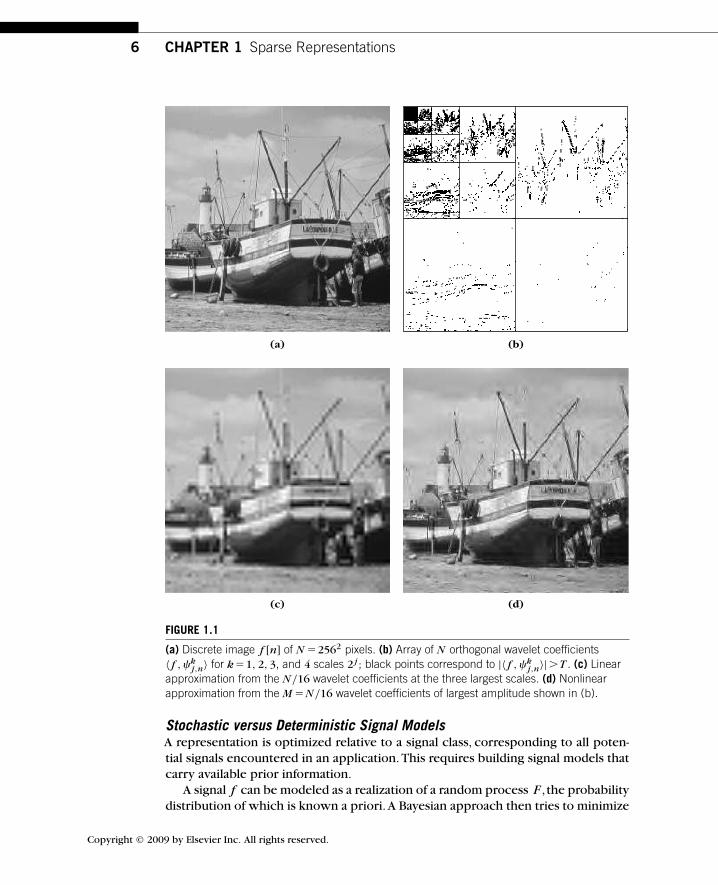
FIGURE 1.1

(a) Discrete image f [n] of N �2562 pixels. (b) Array of N orthogonal wavelet coefficients〈 f , �k

j,n〉 for k�1, 2, 3, and 4 scales 2 j ; black points correspond to |〈 f , �kj,n〉|T . (c) Linear

approximation from the N/16 wavelet coefficients at the three largest scales. (d) Nonlinearapproximation from the M �N/16 wavelet coefficients of largest amplitude shown in (b).

Stochastic versus Deterministic Signal ModelsA representation is optimized relative to a signal class, corresponding to all poten-tial signals encountered in an application. This requires building signal models thatcarry available prior information.

A signal f can be modeled as a realization of a random process F , the probabilitydistribution of which is known a priori.A Bayesian approach then tries to minimize


“Mallat: 05-ch01-p374370” — 2009/3/7 — 17:59 — page 7 — #7


the expected approximation error. Linear approximations are simpler because theyonly depend on the covariance. Chapter 9 shows that optimal linear approxima-tions are obtained on the basis of principal components that are the eigenvectorsof the covariance matrix. However,the expected error of nonlinear approximationsdepends on the full probability distribution of F . This distribution is most oftennot known for complex signals, such as images or sounds, because their transientstructures are not adequately modeled as realizations of known processes such asGaussian ones.

To optimize nonlinear representations, weaker but sufficiently powerful deter-ministic models can be elaborated. A deterministic model specifies a set �, wherethe signal belongs.This set is defined by any prior information—for example,on thetime-frequency localization of transients in musical recordings or on the geometricregularity of edges in images. Simple models can also define � as a ball in a functionalspace, with a specific regularity norm such as a total variation norm. A stochasticmodel is richer because it provides the probability distribution in �. When this dis-tribution is not available, the average error cannot be calculated and is replaced bythe maximum error over �. Optimizing the representation then amounts to mini-mizing this maximum error, which is called a minimax optimization.

1.2.1 Sampling with Linear ApproximationsAnalog-to-digital signal conversion is most often implemented with a linear approxi-mation operator that filters and samples the input analog signal. From these samples,a linear digital-to-analog converter recovers a projection of the original analog signalover an approximation space whose dimension depends on the sampling density.Linear approximations project signals in spaces of lowest possible dimensions toreduce computations and storage cost, while controlling the resulting error.

Sampling TheoremsLet us consider finite energy signals ‖ f ‖2 �

∫ | f (x)|2 dx of finite support, which isnormalized to [0, 1] or [0, 1]2 for images.A sampling process implements a filteringof f (x) with a low-pass impulse response �s(x) and a uniform sampling to outputa discrete signal:

f [n]� f � �s(ns) for 0�n�N .

In two dimensions,n�(n1, n2) and x �(x1, x2). These filtered samples can also bewritten as inner products:

f � �s(ns)�

∫f (u) �s(ns �u) du� 〈 f (x), �s(x �ns)〉

with �s(x)� �s(�x). Chapter 3 explains that �s is chosen, like in the clas-sic Shannon–Whittaker sampling theorem, so that a family of functions {�s

(x �ns)}1�n�N is a basis of an appropriate approximation space UN . The best lin-ear approximation of f in UN recovered from these samples is the orthogonal


“Mallat: 05-ch01-p374370” — 2009/3/7 — 17:59 — page 8 — #8


projection fN of f in UN , and if the basis is orthonormal, then

fN (x)�

N�1∑n�0

f [n] �s(x �ns). (1.4)

A sampling theorem states that if f ∈UN then f � fN so (1.4) recovers f (x)

from the measured samples. Most often, f does not belong to this approximationspace. It is called aliasing in the context of Shannon–Whittaker sampling, whereUN is the space of functions having a frequency support restricted to the N lowerfrequencies. The approximation error ‖ f � fN‖2 must then be controlled.

Linear Approximation ErrorThe approximation error is computed by finding an orthogonal basis B�{gm(x)}0�m�� of the whole analog signal space L2[0, 1]2, with the first N vec-tor {gm(x)}0�m�N that defines an orthogonal basis of UN . Thus, the orthogonalprojection on UN can be rewritten as

fN (x)�

N�1∑m�0

〈 f , gm〉 gm(x).

Since f �∑��

m�0 〈 f , gm〉 gm, the approximation error is the energy of the removedinner products:

�l(N , f )�‖ f � fN ‖2 �

��∑m�N

|〈 f , gm〉|2.

This error decreases quickly when N increases if the coefficient amplitudes |〈 f , gm〉|have a fast decay when the index m increases. The dimension N is adjusted to thedesired approximation error.

Figure 1.1(a) shows a discrete image f [n] approximated with N �2562 pixels.Figure 1.1(c) displays a lower-resolution image fN/16 projected on a space UN/16 ofdimension N/16,generated by N/16 large-scale wavelets. It is calculated by settingall the wavelet coefficients to zero at the first two smaller scales.The approximationerror is ‖ f � fN/16‖2/‖ f ‖2 �14 10�3. Reducing the resolution introduces moreblur and errors. A linear approximation space UN corresponds to a uniform gridthat approximates precisely uniform regular signals. Since images f are often notuniformly regular, it is necessary to measure it at a high-resolution N . This is whydigital cameras have a resolution that increases as technology improves.

1.2.2 Sparse Nonlinear ApproximationsLinear approximations reduce the space dimensionality but can introduce importanterrors when reducing the resolution if the signal is not uniformly regular, as shownby Figure 1.1(c). To improve such approximations, more coefficients should bekept where needed—not in regular regions but near sharp transitions and edges.


“Mallat: 05-ch01-p374370” — 2009/3/7 — 17:59 — page 9 — #9


This requires defining an irregular sampling adapted to the local signal regularity.This optimized irregular sampling has a simple equivalent solution through nonlinearapproximations in wavelet bases.

Nonlinear approximations operate in two stages. First, a linear operator approx-imates the analog signal f with N samples written f [n]� f � �s(ns). Then, anonlinear approximation of f [n] is computed to reduce the N coefficients f [n]to M �N coefficients in a sparse representation.

The discrete signal f can be considered as a vector of CN. Inner products and

norms in CN are written

〈 f , g〉�

N�1∑n�0

f [n] g∗[n] and ‖ f ‖2 �

N�1∑n�0

| f [n]|2.

To obtain a sparse representation with a nonlinear approximation,we choose a neworthonormal basis B� {gm[n]}m∈� of C

N , which concentrates the signal energy asmuch as possible over few coefficients. Signal coefficients {〈 f , gm〉}m∈� are com-puted from the N input sample values f [n] with an orthogonal change of basisthat takes N2 operations in nonstructured bases. In a wavelet or Fourier bases, fastalgorithms require, respectively, O(N ) and O(N log2 N ) operations.

Approximation by ThresholdingFor M �N ,an approximation fM is computed by selecting the“best”M �N vectorswithin B. The orthogonal projection of f on the space V generated by M vectors{gm}m∈ in B is

f �∑m∈

〈 f , gm〉 gm. (1.5)

Since f �∑

m∈� 〈 f , gm〉 gm, the resulting error is

‖ f � f ‖2 �∑m/∈

|〈 f , gm〉|2. (1.6)

We write | | the size of the set . The best M � | | term approximation, whichminimizes ‖ f � f ‖2, is thus obtained by selecting the M coefficients of largestamplitude. These coefficients are above a threshold T that depends on M :

fM � f T �∑

m∈ T

〈 f , gm〉 gm with T � {m∈� : |〈 f , gm〉|�T }. (1.7)

This approximation is nonlinear because the approximation set T changes withf . The resulting approximation error is:

�n(M, f )�‖ f � fM‖2 �∑

m/∈ T

|〈 f , gm〉|2. (1.8)

Figure 1.1(b) shows that the approximation support T of an image in a waveletorthonormal basis depends on the geometry of edges and textures. Keeping large


“Mallat: 05-ch01-p374370” — 2009/3/7 — 17:59 — page 10 — #10


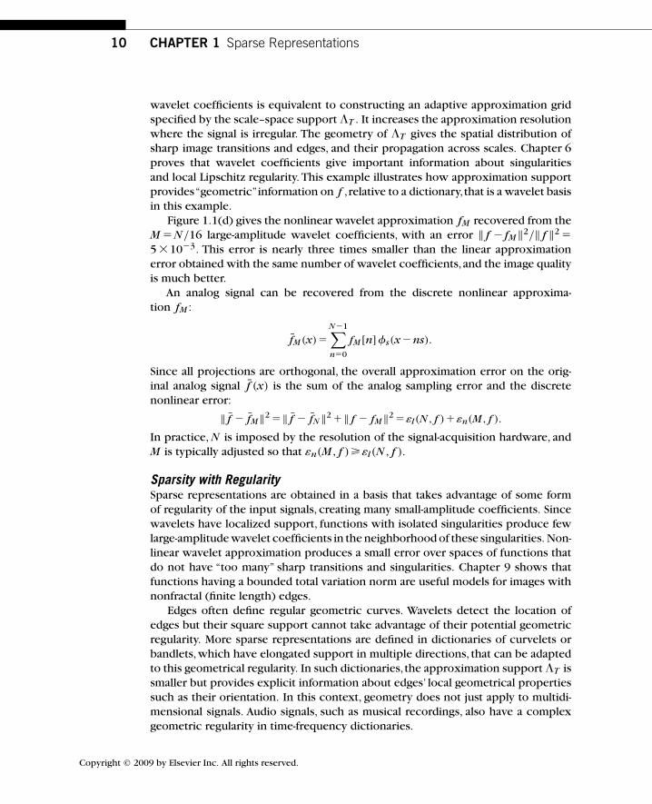
wavelet coefficients is equivalent to constructing an adaptive approximation gridspecified by the scale–space support T . It increases the approximation resolutionwhere the signal is irregular. The geometry of T gives the spatial distribution ofsharp image transitions and edges, and their propagation across scales. Chapter 6proves that wavelet coefficients give important information about singularitiesand local Lipschitz regularity. This example illustrates how approximation supportprovides“geometric”information on f ,relative to a dictionary,that is a wavelet basisin this example.

Figure 1.1(d) gives the nonlinear wavelet approximation fM recovered from theM �N/16 large-amplitude wavelet coefficients, with an error ‖ f � fM‖2/‖ f ‖2 �5 10�3. This error is nearly three times smaller than the linear approximationerror obtained with the same number of wavelet coefficients,and the image qualityis much better.

An analog signal can be recovered from the discrete nonlinear approxima-tion fM :

fM (x)�

N�1∑n�0

fM [n] �s(x �ns).

Since all projections are orthogonal, the overall approximation error on the orig-inal analog signal f (x) is the sum of the analog sampling error and the discretenonlinear error:

‖ f � fM‖2 �‖ f � fN ‖2 �‖ f � fM‖2 ��l(N , f )��n(M, f ).

In practice, N is imposed by the resolution of the signal-acquisition hardware, andM is typically adjusted so that �n(M, f )��l(N , f ).

Sparsity with RegularitySparse representations are obtained in a basis that takes advantage of some formof regularity of the input signals, creating many small-amplitude coefficients. Sincewavelets have localized support, functions with isolated singularities produce fewlarge-amplitude wavelet coefficients in the neighborhood of these singularities. Non-linear wavelet approximation produces a small error over spaces of functions thatdo not have “too many” sharp transitions and singularities. Chapter 9 shows thatfunctions having a bounded total variation norm are useful models for images withnonfractal (finite length) edges.

Edges often define regular geometric curves. Wavelets detect the location ofedges but their square support cannot take advantage of their potential geometricregularity. More sparse representations are defined in dictionaries of curvelets orbandlets,which have elongated support in multiple directions, that can be adaptedto this geometrical regularity. In such dictionaries,the approximation support T issmaller but provides explicit information about edges’ local geometrical propertiessuch as their orientation. In this context, geometry does not just apply to multidi-mensional signals. Audio signals, such as musical recordings, also have a complexgeometric regularity in time-frequency dictionaries.


“Mallat: 05-ch01-p374370” — 2009/3/7 — 17:59 — page 11 — #11


1.2.3 CompressionStorage limitations and fast transmission through narrow bandwidth channelsrequire compression of signals while minimizing degradation. Transform codescompress signals by coding a sparse representation. Chapter 10 introduces theinformation theory needed to understand these codes and to optimize theirperformance.

In a compression framework, the analog signal has already been discretized intoa signal f [n] of size N . This discrete signal is decomposed in an orthonormal basisB� {gm}m∈� of C

N :

f �∑m∈�

〈 f , gm〉 gm.

Coefficients 〈 f , gm〉 are approximated by quantized values Q(〈 f , gm〉). If Q is auniform quantizer of step �, then |x �Q(x)|��/2; and if |x|��/2, then Q(x)�0.The signal f restored from quantized coefficients is

f �∑m∈�

Q(〈 f , gm〉) gm.

An entropy code records these coefficients with R bits. The goal is to minimize thesignal-distortion rate d(R, f )�‖ f � f ‖2.

The coefficients not quantized to zero correspond to the set T � {m∈� :|〈 f , gm〉|�T } with T ��/2. For sparse signals,Chapter 10 shows that the bit budgetR is dominated by the number of bits to code T in �,which is nearly proportionalto its size | T |. This means that the “information” about a sparse representation ismostly geometric. Moreover, the distortion is dominated by the nonlinear approxi-mation error ‖ f � f T ‖2, for f T �

∑m∈ T

〈 f , gm〉gm. Compression is thus a sparseapproximation problem. For a given distortion d(R, f ), minimizing R requiresreducing | T | and thus optimizing the sparsity.

The number of bits to code T can take advantage of any prior information onthe geometry. Figure 1.1(b) shows that large wavelet coefficients are not randomlydistributed.They have a tendency to be aggregated toward larger scales, and at finescales they are regrouped along edge curves or in texture regions. Using such priorgeometric models is a source of gain in coders such as JPEG-2000.

Chapter 10 describes the implementation of audio transform codes. Image trans-form codes in block cosine bases and wavelet bases are introduced, together withthe JPEG and JPEG-2000 compression standards.

1.2.4 DenoisingSignal-acquisition devices add noise that can be reduced by estimators using priorinformation on signal properties. Signal processing has long remained mostlyBayesian and linear. Nonlinear smoothing algorithms existed in statistics, butthese procedures were often ad hoc and complex. Two statisticians, Donoho andJohnstone [221], changed the“game”by proving that simple thresholding in sparse


“Mallat: 05-ch01-p374370” — 2009/3/7 — 17:59 — page 12 — #12


representations can yield nearly optimal nonlinear estimators. This was the begin-ning of a considerable refinement of nonlinear estimation algorithms that is stillongoing.

Let us consider digital measurements that add a random noise W [n] to theoriginal signal f [n]:

X[n]� f [n]�W [n] for 0�n�N .

The signal f is estimated by transforming the noisy data X with an operator D:

F �DX .

The risk of the estimator F of f is the average error, calculated with respect to theprobability distribution of noise W :

r(D, f )�E{‖ f �DX‖2}.

Bayes versus MinimaxTo optimize the estimation operator D,one must take advantage of prior informationavailable about signal f . In a Bayes framework, f is considered a realization of arandom vector F and the Bayes risk is the expected risk calculated with respect tothe prior probability distribution � of the random signal model F :

r(D, �)�E�{r(D, F)}.Optimizing D among all possible operators yields the minimum Bayes risk:

rn(�)� infall D

r(D, �).

In the 1940s,Wald brought in a new perspective on statistics with a decision the-ory partly imported from the theory of games.This point of view uses deterministicmodels, where signals are elements of a set �, without specifying their probabilitydistribution in this set.To control the risk for any f ∈�,we compute the maximumrisk:

r(D, �)�supf ∈�

r(D, f ).

The minimax risk is the lower bound computed over all operators D:

rn(�)� infall D

r(D, �).

In practice, the goal is to find an operator D that is simple to implement and yieldsa risk close to the minimax lower bound.

Thresholding EstimatorsIt is tempting to restrict calculations to linear operators D because of their simplicity.Optimal linear Wiener estimators are introduced in Chapter 11. Figure 1.2(a) is animage contaminated by Gaussian white noise. Figure 1.2(b) shows an optimized


“Mallat: 05-ch01-p374370” — 2009/3/7 — 17:59 — page 13 — #13


(a) (b)

(c) (d)

FIGURE 1.2

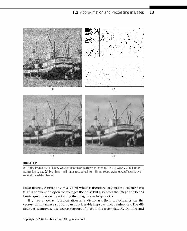
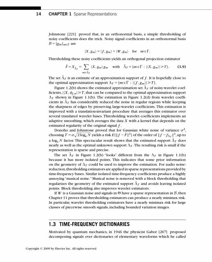
(a) Noisy image X . (b) Noisy wavelet coefficients above threshold, |〈X, �j,n〉|�T . (c) Linearestimation X � h. (d) Nonlinear estimator recovered from thresholded wavelet coefficients overseveral translated bases.

linear filtering estimation F �X � h[n],which is therefore diagonal in a Fourier basisB. This convolution operator averages the noise but also blurs the image and keepslow-frequency noise by retaining the image’s low frequencies.

If f has a sparse representation in a dictionary, then projecting X on thevectors of this sparse support can considerably improve linear estimators. The dif-ficulty is identifying the sparse support of f from the noisy data X . Donoho and


“Mallat: 05-ch01-p374370” — 2009/3/7 — 17:59 — page 14 — #14


Johnstone [221] proved that, in an orthonormal basis, a simple thresholding ofnoisy coefficients does the trick. Noisy signal coefficients in an orthonormal basisB� {gm}m∈� are

〈X, gm〉� 〈 f , gm〉� 〈W, gm〉 for m∈�.

Thresholding these noisy coefficients yields an orthogonal projection estimator

F �X T

�∑

m∈ T

〈X, gm〉 gm with T � {m∈� : |〈X, gm〉|�T }. (1.9)

The set T is an estimate of an approximation support of f . It is hopefully close tothe optimal approximation support T � {m∈� : |〈 f , gm〉|�T }.

Figure 1.2(b) shows the estimated approximation set T of noisy-wavelet coef-ficients, |〈X, �j,n|�T , that can be compared to the optimal approximation support T shown in Figure 1.1(b). The estimation in Figure 1.2(d) from wavelet coeffi-cients in T has considerably reduced the noise in regular regions while keepingthe sharpness of edges by preserving large-wavelet coefficients. This estimation isimproved with a translation-invariant procedure that averages this estimator overseveral translated wavelet bases. Thresholding wavelet coefficients implements anadaptive smoothing, which averages the data X with a kernel that depends on theestimated regularity of the original signal f .

Donoho and Johnstone proved that for Gaussian white noise of variance �2,choosing T ��

√2 loge N yields a risk E{‖ f � F‖2} of the order of ‖ f � f T ‖2,up to

a loge N factor. This spectacular result shows that the estimated support T doesnearly as well as the optimal unknown support T . The resulting risk is small if therepresentation is sparse and precise.

The set T in Figure 1.2(b) “looks” different from the T in Figure 1.1(b)because it has more isolated points. This indicates that some prior informationon the geometry of T could be used to improve the estimation. For audio noise-reduction,thresholding estimators are applied in sparse representations provided bytime-frequency bases. Similar isolated time-frequency coefficients produce a highlyannoying “musical noise.” Musical noise is removed with a block thresholding thatregularizes the geometry of the estimated support T and avoids leaving isolatedpoints. Block thresholding also improves wavelet estimators.

If W is a Gaussian noise and signals in � have a sparse representation in B, thenChapter 11 proves that thresholding estimators can produce a nearly minimax risk.In particular, wavelet thresholding estimators have a nearly minimax risk for largeclasses of piecewise smooth signals, including bounded variation images.

1.3 TIME-FREQUENCY DICTIONARIESMotivated by quantum mechanics, in 1946 the physicist Gabor [267] proposeddecomposing signals over dictionaries of elementary waveforms which he called


“Mallat: 05-ch01-p374370” — 2009/3/7 — 17:59 — page 15 — #15

1.3 Time-Frequency Dictionaries 15

time-frequency atoms that have a minimal spread in a time-frequency plane.By showing that such decompositions are closely related to our perception ofsounds, and that they exhibit important structures in speech and music recordings,Gabor demonstrated the importance of localized time-frequency signal process-ing. Beyond sounds, large classes of signals have sparse decompositions as sums oftime-frequency atoms selected from appropriate dictionaries. The key issue is tounderstand how to construct dictionaries with time-frequency atoms adapted tosignal properties.

1.3.1 Heisenberg UncertaintyA time-frequency dictionary D� {��}�∈� is composed of waveforms of unit norm‖��‖�1, which have a narrow localization in time and frequency. The time locali-zation u of �� and its spread around u, are defined by

u�

∫t|��(t)|2 dt and �2

t,� �

∫|t �u|2 |��(t)|2 dt.

Similarly, the frequency localization and spread of �� are defined by

�(2�)�1∫

�|��(�)|2 d� and �2�,� �(2�)�1

∫|��|2 |��(�)|2 d�.

The Fourier Parseval formula

〈 f , ��〉�

∫ ��

��f (t) �∗

�(t) dt �1

2�

∫ ��

��f (�) �∗

�(�) d� (1.10)

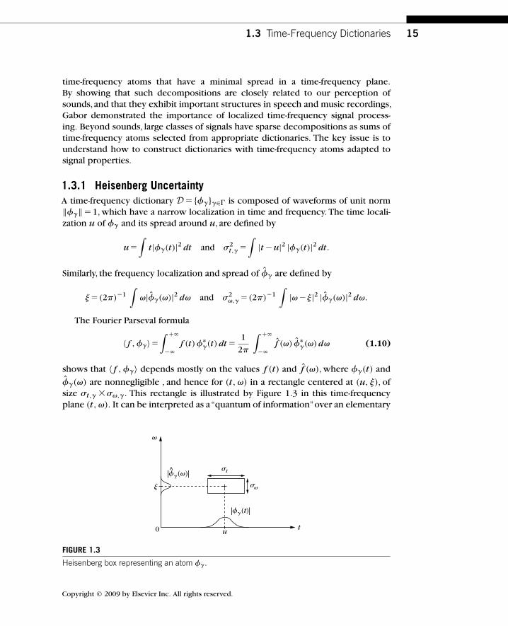
shows that 〈 f , ��〉 depends mostly on the values f (t) and f (�), where ��(t) and

��(�) are nonnegligible , and hence for (t, �) in a rectangle centered at (u, ), ofsize �t,� ��,� . This rectangle is illustrated by Figure 1.3 in this time-frequencyplane (t, �). It can be interpreted as a“quantum of information”over an elementary

u

0 t

�

|�� (t)|

|�� (�)| �t

��

^

FIGURE 1.3

Heisenberg box representing an atom �� .


“Mallat: 05-ch01-p374370” — 2009/3/7 — 17:59 — page 16 — #16


resolution cell. The uncertainty principle theorem proves (see Chapter 2) that thisrectangle has a minimum surface that limits the joint time-frequency resolution:

�t,� ��,� �1

2. (1.11)

Constructing a dictionary of time-frequency atoms can thus be thought of ascovering the time-frequency plane with resolution cells having a time width �t,� anda frequency width ��,� which may vary but with a surface larger than one-half.Windowed Fourier and wavelet transforms are two important examples.

1.3.2 Windowed Fourier TransformA windowed Fourier dictionary is constructed by translating in time and frequencya time window g(t), of unit norm ‖g‖�1, centered at t �0:

D�{gu,(t)�g(t �u) eit

}(u,)∈R2

.

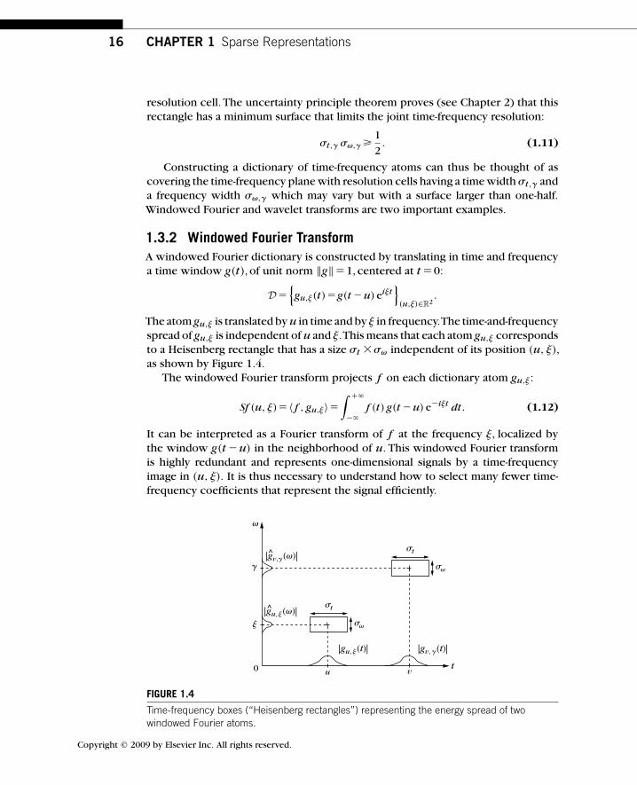
The atom gu, is translated by u in time and by in frequency.The time-and-frequencyspread of gu, is independent of u and .This means that each atom gu, correspondsto a Heisenberg rectangle that has a size �t �� independent of its position (u, ),as shown by Figure 1.4.

The windowed Fourier transform projects f on each dictionary atom gu, :

Sf (u, )� 〈 f , gu,〉�

∫ ��

��f (t) g(t �u) e�it dt. (1.12)

It can be interpreted as a Fourier transform of f at the frequency , localized bythe window g(t �u) in the neighborhood of u. This windowed Fourier transformis highly redundant and represents one-dimensional signals by a time-frequencyimage in (u, ). It is thus necessary to understand how to select many fewer time-frequency coefficients that represent the signal efficiently.

�

0 t

�

|gv,� (�)|

|gu, (�)|

|gv, � (t)||gu, (t)|

^

^

�t

��

�t

��

u v

FIGURE 1.4

Time-frequency boxes (“Heisenberg rectangles”) representing the energy spread of twowindowed Fourier atoms.


“Mallat: 05-ch01-p374370” — 2009/3/7 — 17:59 — page 17 — #17


When listening to music, we perceive sounds that have a frequency that variesin time. Chapter 4 shows that a spectral line of f creates high-amplitude win-dowed Fourier coefficients Sf (u, ) at frequencies (u) that depend on time u.These spectral components are detected and characterized by ridge points, whichare local maxima in this time-frequency plane. Ridge points define a time-frequencyapproximation support of f with a geometry that depends on the time-frequencyevolution of the signal spectral components. Modifying the sound duration or audiotranspositions are implemented by modifying the geometry of the ridge support intime frequency.

A windowed Fourier transform decomposes signals over waveforms that havethe same time and frequency resolution. It is thus effective as long as the signal doesnot include structures having different time-frequency resolutions,some being verylocalized in time and others very localized in frequency. Wavelets address this issueby changing the time and frequency resolution.

1.3.3 Continuous Wavelet TransformIn reflection seismology,Morlet knew that the waveforms sent underground have aduration that is too long at high frequencies to separate the returns of fine, closelyspaced geophysical layers. Such waveforms are called wavelets in geophysics.Instead of emitting pulses of equal duration, he thought of sending shorter wave-forms at high frequencies. These waveforms were obtained by scaling the motherwavelet, hence the name of this transform. Although Grossmann was working intheoretical physics, he recognized in Morlet’s approach some ideas that were closeto his own work on coherent quantum states.

Nearly forty years after Gabor, Morlet and Grossmann reactivated a fundamen-tal collaboration between theoretical physics and signal processing, which led tothe formalization of the continuous wavelet transform [288]. These ideas were nottotally new to mathematicians working in harmonic analysis,or to computer visionresearchers studying multiscale image processing. It was thus only the beginning ofa rapid catalysis that brought together scientists with very different backgrounds.

A wavelet dictionary is constructed from a mother wavelet � of zero average∫ ��

��(t) dt �0,

which is dilated with a scale parameter s, and translated by u:

D�{

�u,s(t)�1√s

�

(t �u

s

)}u∈R,s0

. (1.13)

The continuous wavelet transform of f at any scale s and position u is the projectionof f on the corresponding wavelet atom:

W f (u, s)� 〈 f , �u,s〉�

∫ ��

��f (t)

1√s

�∗(

t �u

s

)dt. (1.14)

It represents one-dimensional signals by highly redundant time-scale images in (u, s).


“Mallat: 05-ch01-p374370” — 2009/3/7 — 17:59 — page 18 — #18


Varying Time-Frequency ResolutionAs opposed to windowed Fourier atoms, wavelets have a time-frequency reso-lution that changes. The wavelet �u,s has a time support centered at u andproportional to s. Let us choose a wavelet � whose Fourier transform �(�) isnonzero in a positive frequency interval centered at . The Fourier transform �u,s(�)

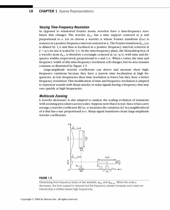
is dilated by 1/s and thus is localized in a positive frequency interval centered at �/s; its size is scaled by 1/s. In the time-frequency plane, the Heisenberg box ofa wavelet atom �u,s is therefore a rectangle centered at (u, /s), with time and fre-quency widths, respectively, proportional to s and 1/s. When s varies, the time andfrequency width of this time-frequency resolution cell changes,but its area remainsconstant, as illustrated by Figure 1.5.

Large-amplitude wavelet coefficients can detect and measure short high-frequency variations because they have a narrow time localization at high fre-quencies. At low frequencies their time resolution is lower, but they have a betterfrequency resolution.This modification of time and frequency resolution is adaptedto represent sounds with sharp attacks,or radar signals having a frequency that mayvary quickly at high frequencies.

Multiscale ZoomingA wavelet dictionary is also adapted to analyze the scaling evolution of transientswith zooming procedures across scales. Suppose now that � is real. Since it has a zeroaverage,a wavelet coefficient Wf (u, s) measures the variation of f in a neighborhoodof u that has a size proportional to s. Sharp signal transitions create large-amplitudewavelet coefficients.

|�u, s (�)|

�u, s �u0, s0

^

|�u0, s0(�)|^

0 t

�

u u0

��s

��

s0�t

s0

s

s0

s �t

FIGURE 1.5

Heisenberg time-frequency boxes of two wavelets, �u,s and �u0,s0 . When the scale sdecreases, the time support is reduced but the frequency spread increases and covers aninterval that is shifted toward high frequencies.


“Mallat: 05-ch01-p374370” — 2009/3/7 — 17:59 — page 19 — #19


Signal singularities have specific scaling invariance characterized by Lipschitzexponents. Chapter 6 relates the pointwise regularity of f to the asymptotic decayof the wavelet transform amplitude |Wf (u, s)| when s goes to zero. Singulari-ties are detected by following the local maxima of the wavelet transform acrossscales.

In images,wavelet local maxima indicate the position of edges,which are sharpvariations of image intensity. It defines scale–space approximation support of ffrom which precise image approximations are reconstructed. At different scales,the geometry of this local maxima support provides contours of image structuresof varying sizes. This multiscale edge detection is particularly effective for patternrecognition in computer vision [146].

The zooming capability of the wavelet transform not only locates isolated sin-gular events, but can also characterize more complex multifractal signals havingnonisolated singularities. Mandelbrot [41] was the first to recognize the existenceof multifractals in most corners of nature. Scaling one part of a multifractal pro-duces a signal that is statistically similar to the whole.This self-similarity appears inthe continuous wavelet transform, which modifies the analyzing scale. From globalmeasurements of the wavelet transform decay, Chapter 6 measures the singular-ity distribution of multifractals. This is particularly important in analyzing theirproperties and testing multifractal models in physics or in financial time series.

1.3.4 Time-Frequency Orthonormal BasesOrthonormal bases of time-frequency atoms remove all redundancy and define sta-ble representations.A wavelet orthonormal basis is an example of the time-frequencybasis obtained by scaling a wavelet � with dyadic scales s �2 j and translating it by2 jn, which is written �j,n. In the time-frequency plane, the Heisenberg resolutionbox of �j,n is a dilation by 2 j and translation by 2 jn of the Heisenberg box of �.A wavelet orthonormal is thus a subdictionary of the continuous wavelet transformdictionary, which yields a perfect tiling of the time-frequency plane illustrated inFigure 1.6.

One can construct many other orthonormal bases of time-frequency atoms,cor-responding to different tilings of the time-frequency plane.Wavelet packet and localcosine bases are two important examples constructed in Chapter 8, with time-frequency atoms that split the frequency and the time axis, respectively, in intervalsof varying sizes.

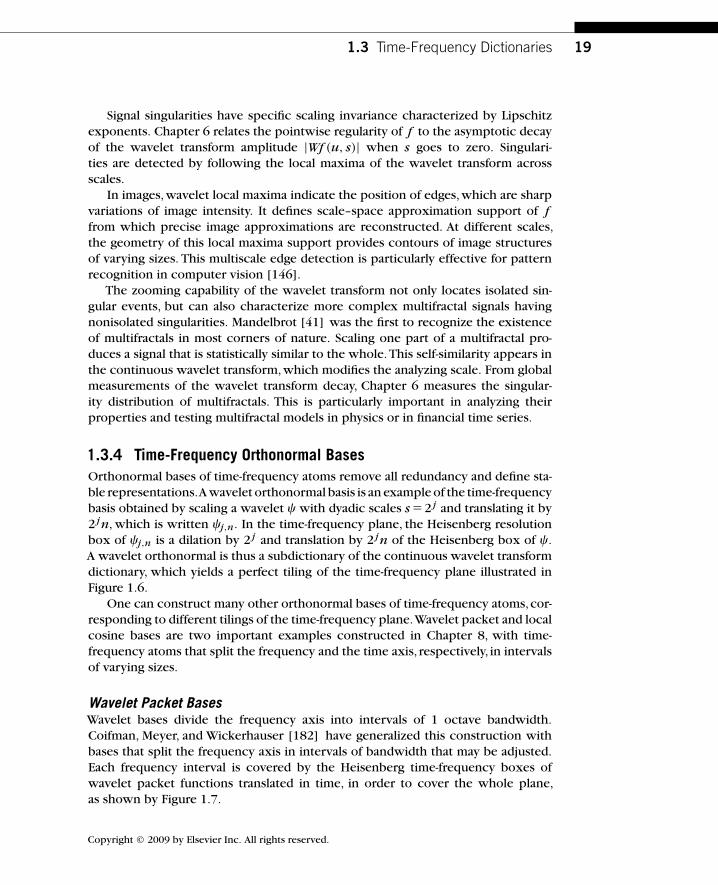
Wavelet Packet BasesWavelet bases divide the frequency axis into intervals of 1 octave bandwidth.Coifman, Meyer, and Wickerhauser [182] have generalized this construction withbases that split the frequency axis in intervals of bandwidth that may be adjusted.Each frequency interval is covered by the Heisenberg time-frequency boxes ofwavelet packet functions translated in time, in order to cover the whole plane,as shown by Figure 1.7.


“Mallat: 05-ch01-p374370” — 2009/3/7 — 17:59 — page 20 — #20


�j, n(t) �j11, p(t)

t

t

�

FIGURE 1.6

The time-frequency boxes of a wavelet basis define a tiling of the time-frequency plane.

t0

�

FIGURE 1.7

A wavelet packet basis divides the frequency axis in separate intervals of varying sizes. A tilingis obtained by translating in time the wavelet packets covering each frequency interval.

As for wavelets, wavelet-packet coefficients are obtained with a filter bank ofconjugate mirror filters that split the frequency axis in several frequency intervals.Different frequency segmentations correspond to different wavelet packet bases.For images, a filter bank divides the image frequency support in squares of dyadicsizes that can be adjusted.

Local Cosine BasesLocal cosine orthonormal bases are constructed by dividing the time axis insteadof the frequency axis.The time axis is segmented in successive intervals [ap, ap�1].The local cosine bases of Malvar [368] are obtained by designing smooth windowsgp(t) that cover each interval [ap, ap�1], and by multiplying them by cosine func-tions cos(t ��) of different frequencies. This is yet another idea that has beenindependently studied in physics,signal processing,and mathematics. Malvar’s orig-inal construction was for discrete signals. At the same time, the physicist Wilson[486] was designing a local cosine basis, with smooth windows of infinite support,


“Mallat: 05-ch01-p374370” — 2009/3/7 — 17:59 — page 21 — #21

1.4 Sparsity in Redundant Dictionaries 21

0

0

t

t

gp(t)

1p

ap21 ap11ap

�

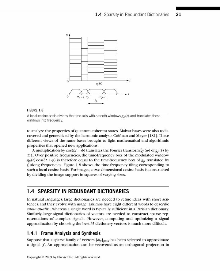
FIGURE 1.8

A local cosine basis divides the time axis with smooth windows gp(t) and translates thesewindows into frequency.

to analyze the properties of quantum coherent states. Malvar bases were also redis-covered and generalized by the harmonic analysts Coifman and Meyer [181].Thesedifferent views of the same bases brought to light mathematical and algorithmicproperties that opened new applications.

A multiplication by cos(t ��) translates the Fourier transform gp(�) of gp(t) by�. Over positive frequencies, the time-frequency box of the modulated windowgp(t) cos(t ��) is therefore equal to the time-frequency box of gp translated by along frequencies. Figure 1.8 shows the time-frequency tiling corresponding tosuch a local cosine basis. For images, a two-dimensional cosine basis is constructedby dividing the image support in squares of varying sizes.

1.4 SPARSITY IN REDUNDANT DICTIONARIESIn natural languages, large dictionaries are needed to refine ideas with short sen-tences, and they evolve with usage. Eskimos have eight different words to describesnow quality, whereas a single word is typically sufficient in a Parisian dictionary.Similarly, large signal dictionaries of vectors are needed to construct sparse rep-resentations of complex signals. However, computing and optimizing a signalapproximation by choosing the best M dictionary vectors is much more difficult.

1.4.1 Frame Analysis and SynthesisSuppose that a sparse family of vectors {�p}p∈ has been selected to approximatea signal f . An approximation can be recovered as an orthogonal projection in


“Mallat: 05-ch01-p374370” — 2009/3/7 — 17:59 — page 22 — #22


the space V generated by these vectors. We then face one of the following twoproblems.

1. In a dual-synthesis problem,the orthogonal projection f of f in V must becomputed from dictionary coefficients, {〈 f , �p〉}p∈ ,provided by an analysisoperator. This is the case when a signal transform {〈 f , �p〉}p∈� is calculated insome large dictionary and a subset of inner products are selected. Such innerproducts may correspond to coefficients above a threshold or local maximavalues.

2. In a dual-analysis problem, the decomposition coefficients of f must becomputed on a family of selected vectors {�p}p∈ . This problem appearswhen sparse representation algorithms select vectors as opposed to innerproducts.This is the case for pursuit algorithms,which compute approxima-tion supports in highly redundant dictionaries.

The frame theory gives energy equivalence conditions to solve both problemswith stable operators.A family {�p}p∈ is a frame of the space V it generates if thereexists B�A0 such that

�h∈V, A‖h‖2 �∑m∈

|〈h, �p〉|2 � B‖h‖2.

The representation is stable since any perturbation of frame coefficients impliesa modification of similar magnitude on h. Chapter 5 proves that the existenceof a dual frame {�p}p∈ that solves both the dual-synthesis and dual-analysisproblems:

f �∑p∈

〈 f , �p〉 �p �∑p∈

〈 f , �p〉 �p. (1.15)

Algorithms are provided to calculate these decompositions. The dual frame is alsostable:

�f ∈ V, B�1‖ f ‖2 �∑m∈�

|〈 f , �p〉|2 � B�1‖ f ‖2.

The frame bounds A and B are redundancy factors. If the vectors {�p}p∈� arenormalized and linearly independent, then A�1�B. Such a dictionary is called aRiesz basis of V and the dual frame is biorthogonal:

�( p, p�)∈ 2, 〈�p, �p�〉��[ p�p�].When the basis is orthonormal, then both bases are equal. Analysis and synthesisproblems are then identical.

The frame theory is also used to construct redundant dictionaries that define com-plete,stable,and redundant signal representations,where V is then the whole signalspace. The frame bounds measure the redundancy of such dictionaries. Chapter 5studies the construction of windowed Fourier and wavelet frame dictionaries by


“Mallat: 05-ch01-p374370” — 2009/3/7 — 17:59 — page 23 — #23


sampling their time, frequency, and scaling parameters, while controlling framebounds. In two dimensions, directional wavelet frames include wavelets sensitiveto directional image structures such as textures or edges.

To improve the sparsity of images having edges along regular geometric curves,Candès and Donoho [134] introduced curvelet frames, with elongated waveformshaving different directions, positions, and scales. Images with piecewise regularedges have representations that are asymptotically more sparse by thresholdingcurvelet coefficients than wavelet coefficients.

1.4.2 Ideal Dictionary ApproximationsIn a redundant dictionary D� {�p}p∈�, we would like to find the best approximationsupport with M � | | vectors, which minimize the error ‖ f � f ‖2. Chapter 12proves that it is equivalent to find T , which minimizes the corresponding appro-ximation Lagrangian

L0(T , f , )�‖ f � f ‖2 �T 2| |, (1.16)

for some multiplier T .Compression and denoising are two applications of redundant dictionary

approximations. When compressing signals by quantizing dictionary coefficients,the distortion rate varies,like the Lagrangian (1.16),with a multiplier T that dependson the quantization step. Optimizing the coder is thus equivalent to minimizing thisapproximation Lagrangian. For sparse representations,most of the bits are devotedto coding the geometry of the sparse approximation set T in �.

Estimators reducing noise from observations X � f �W are also optimized byfinding a best orthogonal projector over a set of dictionary vectors. The modelselection theory of Barron, Birgé, and Massart [97] proves that finding T , whichminimizes this same Lagrangian L0(T , X, ), defines an estimator that has a risk onthe same order as the minimum approximation error ‖ f � f T ‖2 up to a logarithmicfactor. This is similar to the optimality result obtained for thresholding estimatorsin an orthonormal basis.

The bad news is that minimizing the approximation Lagrangian L0 is an NP-hardproblem and is therefore computationally intractable. It is necessary therefore tofind algorithms that are sufficiently fast to compute suboptimal,but “good enough,”solutions.

Dictionaries of Orthonormal BasesTo reduce the complexity of optimal approximations, the search can be reduced tosubfamilies of orthogonal dictionary vectors. In a dictionary of orthonormal bases,any family of orthogonal dictionary vectors can be complemented to form an orthog-onal basis B included in D.As a result, the best approximation of f from orthogonalvectors in B is obtained by thresholding the coefficients of f in a “best basis” in D.

For tree dictionaries of orthonormal bases obtained by a recursive split oforthogonal vector spaces, the fast,dynamic programming algorithm of Coifman and


“Mallat: 05-ch01-p374370” — 2009/3/7 — 17:59 — page 24 — #24


Wickerhauser [182] finds such a best basis with O(P) operations, where P is thedictionary size.

Wavelet packet and local cosine bases are examples of tree dictionaries of time-frequency orthonormal bases of size P �N log2 N . A best basis is a time-frequencytiling that is the best match to the signal time-frequency structures.

To approximate geometrically regular edges, wavelets are not as efficient ascurvelets,but wavelets provide more sparse representations of singularities that arenot distributed along geometrically regular curves. Bandlet dictionaries, introducedby Le Pennec, Mallat, and Peyré [342, 365], are dictionaries of orthonormal basesthat can adapt to the variability of images’ geometric regularity. Minimax optimalasymptotic rates are derived for compression and denoising.

1.4.3 Pursuit in DictionariesApproximating signals only from orthogonal vectors brings rigidity that limits theability to optimize the representation. Pursuit algorithms remove this constraintwith flexible procedures that search for sparse, although not necessarily optimal,dictionary approximations. Such approximations are computed by optimizing thechoice of dictionary vectors {�p}p∈ .

Matching PursuitMatching pursuit algorithms introduced by Mallat and Zhang [366] are greedy algo-rithms that optimize approximations by selecting dictionary vectors one by one.The vector in �p0 ∈D that best approximates a signal f is

�p0 � argmaxp∈�

|〈 f , �p〉|

and the residual approximation error is

Rf � f � 〈 f , �p0〉 �p0 .

A matching pursuit further approximates the residue Rf by selecting anotherbest vector �p1 from the dictionary and continues this process over next-orderresidues Rmf , which produces a signal decomposition:

f �

M�1∑m�0

〈R m f , �pm〉 �pm �R M f .

The approximation from the M -selected vectors {�pm}0�m�M can be refined withan orthogonal back projection on the space generated by these vectors. An orthog-onal matching pursuit further improves this decomposition by orthogonalizingprogressively the projection directions �pm during the decompositon.The resultingdecompositions are applied to compression, denoising, and pattern recognition ofvarious types of signals, images, and videos.


“Mallat: 05-ch01-p374370” — 2009/3/7 — 17:59 — page 25 — #25


Basis PursuitApproximating f with a minimum number of nonzero coefficients a[ p] in a dic-tionary D is equivalent to minimizing the l 0 norm ‖a‖0, which gives the numberof nonzero coefficients.This l 0 norm is highly nonconvex,which explains why theresulting minimization is NP-hard. Donoho and Chen [158] thus proposed replac-ing the l 0 norm by the l1 norm ‖a‖1 �

∑p∈� |a[ p]|, which is convex. The resulting

basis pursuit algorithm computes a synthesis operator

f �∑p∈�

a[ p] �p, which minimizes ‖a‖1 �∑p∈�

|a[ p]|. (1.17)

This optimal solution is calculated with a linear programming algorithm.A basis pursuit is computationally more intense than a matching pursuit, butit is a more global optimization that yields representations that can be moresparse.

In approximation, compression, or denoising applications, f is recovered withan error bounded by a precision parameter �.The optimization (1.18) is thus relaxedby finding a synthesis such that

‖ f �∑p∈�

a[ p] �p‖��, which minimizes ‖a‖1 �∑p∈�

|a[ p]|. (1.18)

This is a convex minimization problem, with a solution calculated by minimizingthe corresponding l1 Lagrangian

L1(T , f , a)�‖ f �∑p∈�

a[ p] �p‖2 �T ‖a‖1,

where T is a Lagrange multiplier that depends on �. This is called an l1 Lagrangianpursuit in this book. A solution a[ p] is computed with iterative algorithms that areguaranteed to converge. The number of nonzero coordinates of a typically decrea-ses as T increases.

Incoherence for Support RecoveryMatching pursuit and l1 Lagrangian pursuits are optimal if they recover the approx-imation support T , which minimizes the approximation Lagrangian

L0(T , f , )�‖ f � f ‖2 �T 2 | |,where f is the orthogonal projection of f in the space V generated by {�p}p∈ .This is not always true and depends on T . An Exact Recovery Criteria proved byTropp [464] guarantees that pursuit algorithms do recover the optimal support T if

ERC( T )� maxq /∈ T

∑p∈ T

|〈�p, �q〉|�1, (1.19)


“Mallat: 05-ch01-p374370” — 2009/3/7 — 17:59 — page 26 — #26


where {�p}p∈ T is the biorthogonal basis of {�p}p∈ T in V T .This criterion impliesthat dictionary vectors �q outside T should have a small inner product with vectorsin T .

This recovery is stable relative to noise perturbations if {�p}p∈ has Riesz boundsthat are not too far from 1. These vectors should be nearly orthogonal and hencehave small inner products. These small inner-product conditions are interpretedas a form of incoherence. A stable recovery of T is possible if vectors in T areincoherent with respect to other dictionary vectors and are incoherent betweenthemselves. It depends on the geometric configuration of T in �.

1.5 INVERSE PROBLEMSMost digital measurement devices, such as cameras, microphones, or medical imag-ing systems, can be modeled as a linear transformation of an incoming analogsignal,plus noise due to intrinsic measurement fluctuations or to electronic noises.This linear transformation can be decomposed into a stable analog-to-digital linearconversion followed by a discrete operator U that carries the specific trans-fer function of the measurement device. The resulting measured data can bewritten

Y [q]�Uf [q]�W [q],

where f ∈CN is the high-resolution signal we want to recover, and W [q] is the

measurement noise. For a camera with an optic that is out of focus, the operatorU is a low-pass convolution producing a blur. For a magnetic resonance imagingsystem, U is a Radon transform integrating the signal along rays and the numberQ of measurements is smaller than N . In such problems, U is not invertible andrecovering an estimate of f is an ill-posed inverse problem.

Inverse problems are among the most difficult signal-processing problems withconsiderable applications. When data acquisition is difficult,costly,or dangerous,orwhen the signal is degraded, super-resolution is important to recover the highestpossible resolution information.This applies to satellite observations,seismic explo-ration,medical imaging,radar,camera phones,or degraded Internet videos displayedon high-resolution screens. Separating mixed information sources from fewer mea-surements is yet another super-resolution problem in telecommunication or audiorecognition.

Incoherence, sparsity, and geometry play a crucial role in the solution of ill-defined inverse problems.With a sensing matrix U with random coefficients,Candèsand Tao [139] and Donoho [217] proved that super-resolution becomes stable forsignals having a sufficiently sparse representation in a dictionary. This remarkableresult opens the door to new compression sensing devices and algorithms thatrecover high-resolution signals from a few randomized linear measurements.


“Mallat: 05-ch01-p374370” — 2009/3/7 — 17:59 — page 27 — #27

1.5 Inverse Problems 27

1.5.1 Diagonal Inverse EstimationIn an ill-posed inverse problem,

Y �Uf �W

the image space ImU � {Uh : h∈CN } of U is of dimension Q smaller than the high-

resolution space N where f belongs. Inverse problems include two difficulties.In the image space ImU, where U is invertible, its inverse may amplify the noiseW , which then needs to be reduced by an efficient denoising procedure. In thenull space NullU, all signals h are set to zero Uh�0 and thus disappear in themeasured data Y . Recovering the projection of f in NullU requires using somestrong prior information. A super-resolution estimator recovers an estimation of fin a dimension space larger than Q and hopefully equal to N , but this is not alwayspossible.

Singular Value DecompositionsLet f �

∑m∈� a[m] gm be the representation of f in an orthonormal basis B�

{gm}m∈�. An approximation must be recovered from

Y �∑m∈�

a[m] Ugm �W .

A basis B of singular vectors diagonalizes U ∗U. Then U transforms a subset of Qvectors {gm}m∈�Q of B into an orthogonal basis {Ugm}m∈�Q of ImU and sets allother vectors to zero. A singular value decomposition estimates the coefficientsa[m] of f by projecting Y on this singular basis and by renormalizing the resultingcoefficients

�m∈�, a[m]�〈Y , Ugm〉

‖Ugm‖2 �h2m

,

where h2m are regularization parameters.

Such estimators recover nonzero coefficients in a space of dimension Q andthus bring no super-resolution. If U is a convolution operator, then B is theFourier basis and a singular value estimation implements a regularized inverseconvolution.

Diagonal Thresholding EstimationThe basis that diagonalizes U ∗U rarely provides a sparse signal representation. Forexample,a Fourier basis that diagonalizes convolution operators does not efficientlyapproximate signals including singularities.

Donoho [214] introduced more flexibility by looking for a basis B providing asparse signal representation,where a subset of Q vectors {gm}m∈�Q are transformedby U in a Riesz basis {Ugm}m∈�Q of ImU, while the others are set to zero. With

an appropriate renormalization,{��1m Ugm}m∈�Q has a biorthogonal basis {�m}m∈�Q


“Mallat: 05-ch01-p374370” — 2009/3/7 — 17:59 — page 28 — #28


that is normalized ‖�m‖�1.The sparse coefficients of f in B can then be estimatedwith a thresholding

�m∈�Q, a[m]� Tm(��1m 〈Y, �m〉) with T (x)�x 1|x|T ,

for thresholds Tm appropriately defined.For classes of signals that are sparse in B, such thresholding estimators may

yield a nearly minimax risk, but they provide no super-resolution since this non-linear projector remains in a space of dimension Q. This result applies to classesof convolution operators U in wavelet or wavelet packet bases. Diagonal inverseestimators are computationally efficient and potentially optimal in cases wheresuper-resolution is not possible.

1.5.2 Super-resolution and Compressive SensingSuppose that f has a sparse representation in some dictionary D� {gp}p∈� ofP normalized vectors. The P vectors of the transformed dictionary DU �UD�{Ugp}p∈� belong to the space ImU of dimension Q�P and thus define a redundantdictionary. Vectors in the approximation support of f are not restricted a priorito a particular subspace of C

N . Super-resolution is possible if the approximationsupport of f in D can be estimated by decomposing the noisy data Y over DU .It depends on the properties of the approximation support of f in �.

Geometric Conditions for Super-resolutionLet w � f � f be the approximation error of a sparse representation f �∑

p∈ a[ p] gp of f . The observed signal can be written as

Y �Uf �W �∑p∈

a[ p] Ugp �Uw �W .

If the support can be identified by finding a sparse approximation of Y in DU

Y �∑p∈

a[ p] Ugp,

then we can recover a super-resolution estimation of f

F �∑p∈

a[ p] gp.

This shows that super-resolution is possible if the approximation support can beidentified by decomposing Y in the redundant transformed dictionary DU . If theexact recovery criteria is satisfy ERC( )�1 and if {Ugp}p∈ is a Riesz basis, then can be recovered using pursuit algorithms with controlled error bounds.

For most operator U, not all sparse approximation sets can be recovered. It isnecessary to impose some further geometric conditions on in �, which makessuper-resolution difficult and often unstable. Numerical applications to sparse spikedeconvolution, tomography, super-resolution zooming, and inpainting illustratethese results.


“Mallat: 05-ch01-p374370” — 2009/3/7 — 17:59 — page 29 — #29

1.5 Inverse Problems 29

Compressive Sensing with RandomnessCandès and Tao [139], and Donoho [217] proved that stable super-resolutionis possible for any sufficiently sparse signal f if U is an operator with randomcoefficients. Compressive sensing then becomes possible by recovering a closeapproximation of f ∈C

N from Q�N linear measurements [133].A recovery is stable for a sparse approximation set | |�M only if the corre-

sponding dictionary family {Ugm}m∈ is a Riesz basis of the space it generates.The M-restricted isometry conditions of Candès,Tao, and Donoho [217] imposesuniform Riesz bounds for all sets ⊂� with | |�M :

�c ∈C| |, (1��M ) ‖c‖2 �‖

∑m∈

c[ p] Ugp‖2 �(1��M ) ‖c‖2. (1.20)

This is a strong incoherence condition on the P vectors of {Ugm}m∈�, which sup-poses that any subset of less than M vectors is nearly uniformly distributed on theunit sphere of ImU.

For an orthogonal basis D� {gm}m∈�, this is possible for M �C Q(log N )�1 ifU is a matrix with independent Gaussian random coefficients. A pursuit algorithmthen provides a stable approximation of any f ∈CN having a sparse approximationfrom vectors in D.

These results open a new compressive-sensing approach to signal acquisition andrepresentation. Instead of first discretizing linearly the signal at a high-resolutionN and then computing a nonlinear representation over M coefficients in somedictionary,compressive-sensing measures directly M randomized linear coefficients.A reconstructed signal is then recovered by a nonlinear algorithm, producing anerror that can be of the same order of magnitude as the error obtained by the moreclassic two-step approximation process,with a more economic acquisiton process.These results remain valid for several types of random matrices U . Examples ofapplications to single-pixel cameras, video super-resolution, new analog-to-digitalconverters, and MRI imaging are described.

Blind Source SeparationSparsity in redundant dictionaries also provides efficient strategies to separate afamily of signals { fs}0�s�S that are linearly mixed in K �S observed signals withnoise:

Yk[n]�

S�1∑s�0

uk,s fs[n]�Wk[n] for 0�n � N and 0�k�K .

From a stereo recording, separating the sounds of S musical instruments is anexample of source separation with k�2. Most often the mixing matrix U �{uk,s}0�k�K ,0�s�S is unknown. Source separation is a super-resolution problemsince S N data values must be recovered from Q�K N �S N measurements. Notknowing the operator U makes it even more complicated.

If each source fs has a sparse approximation support s in a dictionary D,with∑S�1s�0 | s|�N , then it is likely that the sets { s}0�s�s are nearly disjoint. In this


“Mallat: 05-ch01-p374370” — 2009/3/7 — 17:59 — page 30 — #30


case, the operator U , the supports s, and the sources fs are approximated bycomputing sparse approximations of the observed data Yk in D. The distributionof these coefficients identifies the coefficients of the mixing matrix U and thenearly disjoint source supports.Time-frequency separation of sounds illustrate theseresults.

1.6 TRAVEL GUIDE1.6.1 Reproducible Computational ScienceThis book covers the whole spectrum from theorems on functions of continuousvariables to fast discrete algorithms and their applications. Section 1.1.2 arguesthat models based on continuous time functions give useful asymptotic results forunderstanding the behavior of discrete algorithms. Still, a mathematical analysisalone is often unable to fully predict the behavior and suitability of algorithmsfor specific signals. Experiments are necessary and such experiments should bereproducible, just like experiments in other fields of science [124].

The reproducibility of experiments requires having complete software and fullsource code for inspection, modification, and application under varied parame-ter settings. Following this perspective, computational algorithms presented inthis book are available as MATLAB subroutines or in other software packages.Figures can be reproduced and the source code is available. Software demonstra-tions and selected exercise solutions are available at http://wavelet-tour.com. Forthe instructor, solutions are available at www.elsevierdirect.com/9780123743701.

1.6.2 Book Road MapSome redundancy is introduced between sections to avoid imposing a linear pro-gression through the book. The preface describes several possible programs for asparse signal-processing course.

All theorems are explained in the text and reading the proofs is not necessary tounderstand the results. Most of the book’s theorems are proved in detail,and impor-tant techniques are included. Exercises at the end of each chapter give examples ofmathematical, algorithmic, and numeric applications, ordered by level of difficultyfrom 1 to 4, and selected solutions can be found at http://wavelet-tour.com.

The book begins with Chapters 2 and 3, which review the Fourier transformand linear discrete signal processing. They provide the necessary backgroundfor readers with no signal-processing background. Important properties of linearoperators, projectors, and vector spaces can be found in the Appendix. Local time-frequency transforms and dictionaries are presented in Chapter 4; the wavelet andwindowed Fourier transforms are introduced and compared. The measurement ofinstantaneous frequencies illustrates the limitations of time-frequency resolution.Dictionary stability and redundancy are introduced in Chapter 5 through the frametheory,with examples of windowed Fourier,wavelet,and curvelet frames. Chapter 6


“Mallat: 05-ch01-p374370” — 2009/3/7 — 17:59 — page 31 — #31

1.6 Travel Guide 31

explains the relationship between wavelet coefficient amplitude and local signalregularity. It is applied to the detection of singularities and edges and to the analysisof multifractals.

Wavelet bases and fast filter bank algorithms are important tools presented inChapter 7. An overdose of orthonormal bases can strike the reader while study-ing the construction and properties of wavelet packets and local cosine basesin Chapter 8. It is thus important to read Chapter 9, which describes sparseapproximations in bases. Signal-compression and denoising applications describedin Chapters 10 and 11 give life to most theoretical and algorithmic results in thebook. These chapters offer a practical perspective on the relevance of linear andnonlinear signal-processing algorithms. Chapter 12 introduces sparse decomposi-tions in redundant dictionaries and their applications. The resolution of inverseproblems is studied in Chapter 13, with super-resolution, compressive sensing, andsource separation.


“Mallat: 05-ch01-p374370” — 2009/3/7 — 17:59 — page 32 — #32

Documents

Sparse Representations