Sparse Methods for Biomedical Data

Sparse Methods for Biomedical Data

Jieping YeArizona State University

Tempe, AZ 85287

[email protected]

Jun LiuSiemens Corporate Research

Princeton, NJ [email protected]

ABSTRACTFollowing recent technological revolutions, the investigationof massive biomedical data with growing scale, diversity, andcomplexity has taken a center stage in modern data analysis.Although complex, the underlying representations of manybiomedical data are often sparse. For example, for a certaindisease such as leukemia, even though humans have tens ofthousands of genes, only a few genes are relevant to the dis-ease; a gene network is sparse since a regulatory pathwayinvolves only a small number of genes; many biomedical sig-nals are sparse or compressible in the sense that they haveconcise representations when expressed in a proper basis.Therefore, finding sparse representations is fundamentallyimportant for scientific discovery. Sparse methods basedon the `1 norm have attracted a great amount of researchefforts in the past decade due to its sparsity-inducing prop-erty, convenient convexity, and strong theoretical guaran-tees. They have achieved great success in various applica-tions such as biomarker selection, biological network con-struction, and magnetic resonance imaging. In this paper,we review state-of-the-art sparse methods and their appli-cations to biomedical data.

KeywordsSparse learning, structured sparsity, Gaussian graphical model,magnetic resonance imaging

1. INTRODUCTIONRecent technological revolutions have unleashed a torrentof biomedical data with growing scale, diversity, and com-plexity [24; 27; 77; 86; 101]. The wealth of data confrontsscientists with an urgent need for new methods and toolsthat can intelligently and automatically extract useful infor-mation from data and synthesize knowledge [17; 32; 56; 74].Although complex, the underlying representations of manyreal-world data are often sparse [32; 38; 41]. For example,for a certain disease such as leukemia, even though humanshave tens of thousands of genes, only a small number ofthem are relevant to the disease; a gene network is sparsesince a regulatory pathway involves only a small number ofgenes; the neural representation of sounds in the auditorycortex of unanesthetized animals is sparse, since the fractionof neurons active at a given instant is small; many biomed-ical signals have sparse representations when expressed in

a proper basis. Therefore, finding sparse representations isfundamentally important for scientific discovery. The lastdecade has witnessed a growing interest in the search forsparse representations of data.

The quest for sparsity is further motivated for various rea-sons. First, sparse representations enhance the interpretabil-ity of the model. For example, in many biological applica-tions, the selection of genes or proteins which are relatedto the study, is crucial to facilitate the biological interpre-tation [18; 38]. In addition, the resulting gene/protein se-lection might enable a feasible biological validation with areduced experimental cost. Second, sparseness is one way tomeasure the complexity of the learning model [84]. Regu-larization is commonly employed to penalize the complexityof a learning model and alleviate overfitting. Regularizationbased on the `0 norm maximizes sparseness, which, however,leads to an NP-hard problem. As a computationally efficientalternative, the `1 norm regularization, which also leads to asparse model, is widely used in many areas including signalprocessing, statistics, and machine learning [13; 23; 52; 93;98; 124; 127]. Finally, finding sparse representations has re-cently received increasing attention due to the current burstof research in Compressed Sensing (CS) [4; 6; 16; 25; 26;102]. CS is a technique for acquiring and reconstructing asignal utilizing the prior knowledge that it is sparse or com-pressible. It encodes a large sparse signal using a relativelysmall number of linear measurements, and minimizing the`1 norm in order to decode the signal. Recent theories [13;14; 15; 16; 25] assert that one can recover certain signalsand images from far fewer samples or measurements thantraditional methods.

In this paper, we review sparse methods for (1) incorpo-rating a priori knowledge on feature structures for featureselection, (2) constructing undirected Gaussian graphicalmodels, and (3) parallel magnetic resonance imaging.

Structured Feature Selection. Although sparse learn-ing models based on the `1 norm such as the Lasso [98]have achieved great success in many applications, they donot take the existing feature structure into consideration.Specifically, these models yield the same solution after ran-domly reshuffling the features. However, in many applica-tions, the features exhibit certain intrinsic structures, e.g.,spatial or temporal smoothness, disjoint/overlapping groups,trees, and graphs [42; 45; 51; 65; 116]. The a priori struc-ture information may significantly improve the classifica-tion/regression performance and help identify the importantfeatures. For example, in the study of arrayCGH [99; 100],the features—the DNA copy numbers along the genome—

SIGKDD Explorations Volume 14, Issue 1 Page 4

have the natural spatial order, and the fused Lasso, whichincorporates the structure information using an extensionof the `1-norm, outperforms the Lasso in both classifica-tion and feature selection. In this paper, we review variousstructured sparse learning models including group Lasso,sparse group Lasso, overlapping group Lasso, tree Lasso,fused Lasso, and graph Lasso.

Sparse Undirected Gaussian Graphical Models. Undi-rected graphical models explore the relationships among aset of random variables through their joint distribution. Theestimation of undirected graphical models has applicationsin many domains, such as computer vision, biology, andmedicine. An instance is the analysis of gene expressiondata. As shown in many biological studies, genes tend towork in groups based on their biological functions, and thereexist some regulatory relationships between genes [19]. Suchbiological knowledge can be represented as a graph, wherenodes are the genes, and edges describe the regulatory rela-tionships. Graphical models provide a useful tool for mod-eling these relationships, and can be used to explore geneactivities. One of the popular graphical models is the Gaus-sian graphical model (GGM), which assumes the variablesto be Gaussian distributed [5]. In GGM, the problem oflearning a graph is equivalent to estimating the inverse ofthe covariance matrix (precision matrix), since the nonzerooff-diagonal elements of the precision matrix represent edgesin the graph [5]. In some applications, we need to esti-mate multiple related precision matrices. For example, inthe modeling of brain networks for Alzheimer’s disease us-ing neuroimaging data [43], we want to estimate graphicalmodels for three groups: normal controls (NC), patients ofmild cognitive impairment (MCI), and Alzheimer’s patients(AD). These graphs are expected to share some commonconnections, but they are not identical. It is thus desirableto jointly estimate the three graphs. In this paper, we reviewsparse methods for estimating a single undirected graphicalmodel and for estimating multiple related undirected graph-ical models and discuss their properties.

Parallel Magnetic Resonance Imaging. Parallel imag-ing has been the single biggest innovation in magnetic reso-nance imaging in the last decade. It exploits the differencein sensitivities between individual coil elements in a receivearray to reduce the number of gradient encodings requiredfor imaging, and the increase in speed comes at a time whenother approaches to acquisition time reduction were reach-ing engineering and human limits [59]. In the SENSE-typereconstruction approach, researchers have taken advantageof the sparsity promoting penalties (e.g., wavelets and totalvariations) to reduce the acquisition time while maintainingthe image quality. Key components of sparse learning in-clude the estimation of the coil sensitivity profiles, the designof the sparsity promoting regularization, the development ofthe sampling pattern that takes advantage of sparse learn-ing, and the efficient optimization of the non-smooth inverseproblem. In this paper, we review different components ofsparse learning in magnetic resonance imaging.

The rest of the paper is organized as follows. We reviewstructured sparse learning for feature selection in Section 2.The estimation of sparse undirected Gaussian graphical mod-els is presented in Section 3. We discuss sparse learning inparallel magnetic resonance imaging in Section 4. Finally,we conclude the paper in Section 5.

2. STRUCTURED FEATURE SELECTIONWe are given a set of training samples ai, bini=1, whereai ∈ Rp denotes the p-dimensional features for the i-th sam-ple, and bi ∈ R is its response (numeric for regression, andcategorical for classification). In addition, we are given afeature structure, e.g., a group structure, a tree structure,or a graph structure, as part of the input data. We focus ona linear model h : Rp → R with h(a) = xTa, where x ∈ Rpis the vector of model parameters. To fit the model with thetraining samples, we learn the model parameter vector x bysolving the following optimization problem:

minxf(x) ≡ L(x) + λΩ(x), (1)

where L(x) is a loss function, Ω(x) is a regularization termencoding the prior knowledge on the input features, andλ > 0 is the regularization parameter controlling the trade-off between the loss L(·) and the penalty Ω(·).The formulation in (1) can be applied for regression, classi-fication, and longitudinal data analysis:

• Regression: The outcome b is a continuous value, e.g.,the hippocampus volume or the minimental state ex-amination (MMSE) score of a subject in the study ofAlzheimer’s disease. The least squares loss is com-monly used for regression.

• Classification: The outcome b is a discrete value, e.g.,disease status, including normal controls and diseasepatients. The logistic loss is commonly used for clas-sification.

• Longitudinal Data Analysis: The outcome b is the ob-served failure/censoring time. If an event occurs attime t, then the subject has a failure time t. If apatient drops from the study at time t, we considerhe/she is censored at time t. The Cox model is a pop-ular approach for longitudinal data analysis, in whichthe negative log-likelihood function of the proportionalhazard is used as the loss function [21].

The regularization term Ω(x) in (1) is commonly employedto penalize the complexity of a learning model and allevi-ate overfitting, e.g., the `2-norm regularization used in ridgeregression. However, the commonly used `2-norm regular-ization leads to a dense model, i.e., almost all model param-eters in x are non-zero. To enhance the interpretability ofthe model, a sparse model is desired. One popular sparsemodel, known as the Lasso, is based on the `1-norm penalty:

Ωlasso(x) = ‖x‖1. (2)

The Lasso has been applied widely in many biomedical ap-plications [91; 94; 107; 111; 123]. In many applications, thefeatures exhibit certain intrinsic structures, e.g., spatial ortemporal smoothness, graphs, trees, and disjoint/overlappinggroups. The a priori structure information may significantlyimprove the classification/regression performance and helpto identify the important features.

2.1 Group Lasso and Sparse Group LassoIn many applications, the features form a natural groupstructure. For example, the voxels of the positron emissiontomography (PET) images in the Alzheimer’s Disease studycan be divided into a set of non-overlapping groups accord-ing to the brain regions [43]; in the multi-factor ANOVA


Proteomics GWAS PET

Lasso

gLasso

sgLasso

Proteomics GWAS MRIMRI PET

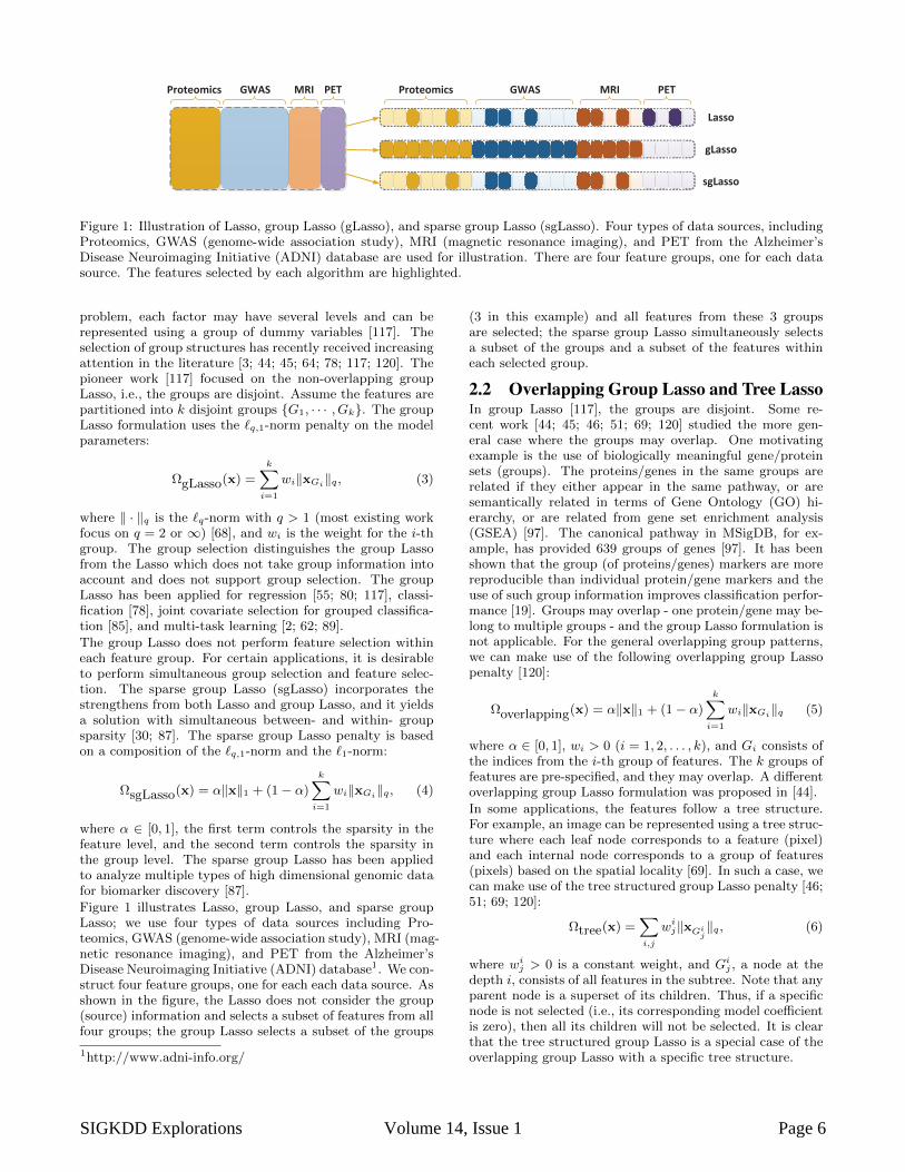
Figure 1: Illustration of Lasso, group Lasso (gLasso), and sparse group Lasso (sgLasso). Four types of data sources, includingProteomics, GWAS (genome-wide association study), MRI (magnetic resonance imaging), and PET from the Alzheimer’sDisease Neuroimaging Initiative (ADNI) database are used for illustration. There are four feature groups, one for each datasource. The features selected by each algorithm are highlighted.

problem, each factor may have several levels and can berepresented using a group of dummy variables [117]. Theselection of group structures has recently received increasingattention in the literature [3; 44; 45; 64; 78; 117; 120]. Thepioneer work [117] focused on the non-overlapping groupLasso, i.e., the groups are disjoint. Assume the features arepartitioned into k disjoint groups G1, · · · , Gk. The groupLasso formulation uses the `q,1-norm penalty on the modelparameters:

ΩgLasso(x) =

k∑i=1

wi‖xGi‖q, (3)

where ‖ · ‖q is the `q-norm with q > 1 (most existing workfocus on q = 2 or ∞) [68], and wi is the weight for the i-thgroup. The group selection distinguishes the group Lassofrom the Lasso which does not take group information intoaccount and does not support group selection. The groupLasso has been applied for regression [55; 80; 117], classi-fication [78], joint covariate selection for grouped classifica-tion [85], and multi-task learning [2; 62; 89].

The group Lasso does not perform feature selection withineach feature group. For certain applications, it is desirableto perform simultaneous group selection and feature selec-tion. The sparse group Lasso (sgLasso) incorporates thestrengthens from both Lasso and group Lasso, and it yieldsa solution with simultaneous between- and within- groupsparsity [30; 87]. The sparse group Lasso penalty is basedon a composition of the `q,1-norm and the `1-norm:

ΩsgLasso(x) = α‖x‖1 + (1− α)

k∑i=1

wi‖xGi‖q, (4)

where α ∈ [0, 1], the first term controls the sparsity in thefeature level, and the second term controls the sparsity inthe group level. The sparse group Lasso has been appliedto analyze multiple types of high dimensional genomic datafor biomarker discovery [87].

Figure 1 illustrates Lasso, group Lasso, and sparse groupLasso; we use four types of data sources including Pro-teomics, GWAS (genome-wide association study), MRI (mag-netic resonance imaging), and PET from the Alzheimer’sDisease Neuroimaging Initiative (ADNI) database1. We con-struct four feature groups, one for each each data source. Asshown in the figure, the Lasso does not consider the group(source) information and selects a subset of features from allfour groups; the group Lasso selects a subset of the groups

1http://www.adni-info.org/

(3 in this example) and all features from these 3 groupsare selected; the sparse group Lasso simultaneously selectsa subset of the groups and a subset of the features withineach selected group.

2.2 Overlapping Group Lasso and Tree LassoIn group Lasso [117], the groups are disjoint. Some re-cent work [44; 45; 46; 51; 69; 120] studied the more gen-eral case where the groups may overlap. One motivatingexample is the use of biologically meaningful gene/proteinsets (groups). The proteins/genes in the same groups arerelated if they either appear in the same pathway, or aresemantically related in terms of Gene Ontology (GO) hi-erarchy, or are related from gene set enrichment analysis(GSEA) [97]. The canonical pathway in MSigDB, for ex-ample, has provided 639 groups of genes [97]. It has beenshown that the group (of proteins/genes) markers are morereproducible than individual protein/gene markers and theuse of such group information improves classification perfor-mance [19]. Groups may overlap - one protein/gene may be-long to multiple groups - and the group Lasso formulation isnot applicable. For the general overlapping group patterns,we can make use of the following overlapping group Lassopenalty [120]:

Ωoverlapping(x) = α‖x‖1 + (1− α)

k∑i=1

wi‖xGi‖q (5)

where α ∈ [0, 1], wi > 0 (i = 1, 2, . . . , k), and Gi consists ofthe indices from the i-th group of features. The k groups offeatures are pre-specified, and they may overlap. A differentoverlapping group Lasso formulation was proposed in [44].

In some applications, the features follow a tree structure.For example, an image can be represented using a tree struc-ture where each leaf node corresponds to a feature (pixel)and each internal node corresponds to a group of features(pixels) based on the spatial locality [69]. In such a case, wecan make use of the tree structured group Lasso penalty [46;51; 69; 120]:

Ωtree(x) =∑i,j

wij‖xGij‖q, (6)

where wij > 0 is a constant weight, and Gij , a node at thedepth i, consists of all features in the subtree. Note that anyparent node is a superset of its children. Thus, if a specificnode is not selected (i.e., its corresponding model coefficientis zero), then all its children will not be selected. It is clearthat the tree structured group Lasso is a special case of theoverlapping group Lasso with a specific tree structure.


0 10 20 30 40 50−1.5

−1

−0.5

0

0.5

1

1.5

λ=0.1, α=0.5

v

x

0 10 20 30 40 50−1.5

−1

−0.5

0

0.5

1

1.5

λ=0.2, α=0.5

v

x

0 10 20 30 40 50−1.5

−1

−0.5

0

0.5

1

1.5

λ=0.3, α=0.5

v

x

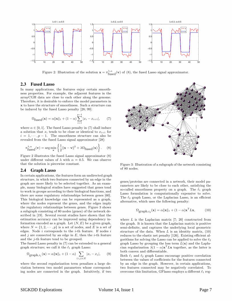
Figure 2: Illustration of the solution x = πλ,αfused

(v) of (8), the fused Lasso signal approximator.

2.3 Fused LassoIn many applications, the features enjoy certain smooth-ness properties. For example, the adjacent features in thearrayCGH data are close to each other along the genome.Therefore, it is desirable to enforce the model parameters inx to have the structure of smoothness. Such a structure canbe induced by the fused Lasso penalty [28; 99]:

Ωfused(x) = α‖x‖1 + (1− α)

p−1∑i=1

|xi − xi+1|, (7)

where α ∈ [0, 1]. The fused Lasso penalty in (7) shall inducea solution that xi tends to be close or identical to xi+1 fori = 1, · · · , p − 1. The smoothness structure can also berevealed from the fused Lasso signal approximator [28]:

πλ,αfused

(v) = arg minx

1

2‖x− v‖2 + λΩfused(x)

. (8)

Figure 2 illustrates the fused Lasso signal approximator (8)under different values of λ with α = 0.5. We can observethat the solution is piecewise constant.

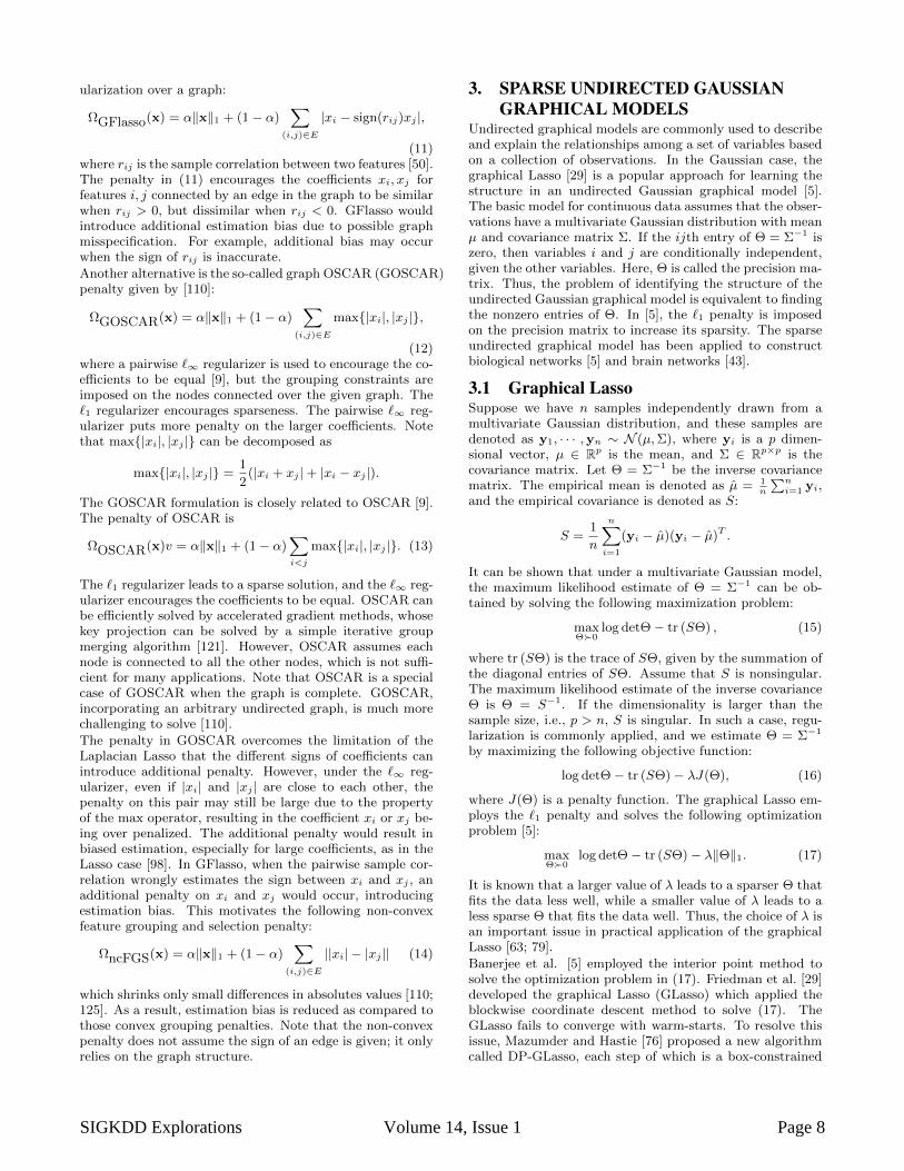
2.4 Graph LassoIn certain applications, the features form an undirected graphstructure, in which two features connected by an edge in thegraph are more likely to be selected together. As an exam-ple, many biological studies have suggested that genes tendto work in groups according to their biological functions, andthere are some regulatory relationships between genes [60].This biological knowledge can be represented as a graph,where the nodes represent the genes, and the edges implythe regulatory relationships between genes. Figure 3 showsa subgraph consisting of 80 nodes (genes) of the network de-scribed in [19]. Several recent studies have shown that theestimation accuracy can be improved using dependency in-formation encoded as a graph. Let (N,E) be a given graph,where N = 1, 2, · · · , p is a set of nodes, and E is a set ofedges. Node i corresponds to the i-th feature. If nodes iand j are connected by an edge in E, then the i-th featureand the j-th feature tend to be grouped.

The fussed Lasso penalty in (7) can be extended to a generalgraph structure; we call it the `1 graph Lasso:

Ωgraph,`1(x) = α‖x‖1 + (1− α)∑

(i,j)∈E

|xi − xj |, (9)

where the second regularization term penalizes a large de-viation between two model parameters whose correspond-ing nodes are connected in the graph. Intuitively, if two

Figure 3: Illustration of a subgraph of the network consistingof 80 nodes.

genes/proteins are connected in a network, their model pa-rameters are likely to be close to each other, satisfying theso-called smoothness property on a graph. The `1 graphLasso formulation is computationally expensive to solve.The `2 graph Lasso, or the Laplacian Lasso, is an efficientalternative, which uses the following penalty:

Ωgraph,`2(x) = α‖x‖1 + (1− α)xTLx, (10)

where L is the Laplacian matrix [7; 20] constructed fromthe graph. It is known that the Laplacian matrix is positivesemi-definite, and captures the underlying local geometricstructure of the data. When L is an identity matrix, (10)reduces to the elastic net penalty [126]. Existing efficient al-gorithms for solving the Lasso can be applied to solve the `2graph Lasso by grouping the loss term L(x) and the Lapla-cian regularization λ(1 − α)xTLx together, as the latter isboth convex and differentiable.

Both `1 and `2 graph Lasso encourage positive correlationbetween the values of coefficients for the features connectedby an edge in the graph. However, in certain applications,two features connected may be negatively correlated. Toovercome this limitation, GFlasso employs a different `1 reg-


ularization over a graph:

ΩGFlasso(x) = α‖x‖1 + (1− α)∑

(i,j)∈E

|xi − sign(rij)xj |,

(11)where rij is the sample correlation between two features [50].The penalty in (11) encourages the coefficients xi, xj forfeatures i, j connected by an edge in the graph to be similarwhen rij > 0, but dissimilar when rij < 0. GFlasso wouldintroduce additional estimation bias due to possible graphmisspecification. For example, additional bias may occurwhen the sign of rij is inaccurate.

Another alternative is the so-called graph OSCAR (GOSCAR)penalty given by [110]:

ΩGOSCAR(x) = α‖x‖1 + (1− α)∑

(i,j)∈E

max|xi|, |xj |,

(12)where a pairwise `∞ regularizer is used to encourage the co-efficients to be equal [9], but the grouping constraints areimposed on the nodes connected over the given graph. The`1 regularizer encourages sparseness. The pairwise `∞ reg-ularizer puts more penalty on the larger coefficients. Notethat max|xi|, |xj | can be decomposed as

max|xi|, |xj | =1

2(|xi + xj |+ |xi − xj |).

The GOSCAR formulation is closely related to OSCAR [9].The penalty of OSCAR is

ΩOSCAR(x)v = α‖x‖1 + (1− α)∑i<j

max|xi|, |xj |. (13)

The `1 regularizer leads to a sparse solution, and the `∞ reg-ularizer encourages the coefficients to be equal. OSCAR canbe efficiently solved by accelerated gradient methods, whosekey projection can be solved by a simple iterative groupmerging algorithm [121]. However, OSCAR assumes eachnode is connected to all the other nodes, which is not suffi-cient for many applications. Note that OSCAR is a specialcase of GOSCAR when the graph is complete. GOSCAR,incorporating an arbitrary undirected graph, is much morechallenging to solve [110].

The penalty in GOSCAR overcomes the limitation of theLaplacian Lasso that the different signs of coefficients canintroduce additional penalty. However, under the `∞ reg-ularizer, even if |xi| and |xj | are close to each other, thepenalty on this pair may still be large due to the propertyof the max operator, resulting in the coefficient xi or xj be-ing over penalized. The additional penalty would result inbiased estimation, especially for large coefficients, as in theLasso case [98]. In GFlasso, when the pairwise sample cor-relation wrongly estimates the sign between xi and xj , anadditional penalty on xi and xj would occur, introducingestimation bias. This motivates the following non-convexfeature grouping and selection penalty:

ΩncFGS(x) = α‖x‖1 + (1− α)∑

(i,j)∈E

||xi| − |xj || (14)

which shrinks only small differences in absolutes values [110;125]. As a result, estimation bias is reduced as compared tothose convex grouping penalties. Note that the non-convexpenalty does not assume the sign of an edge is given; it onlyrelies on the graph structure.

3. SPARSE UNDIRECTED GAUSSIANGRAPHICAL MODELS

Undirected graphical models are commonly used to describeand explain the relationships among a set of variables basedon a collection of observations. In the Gaussian case, thegraphical Lasso [29] is a popular approach for learning thestructure in an undirected Gaussian graphical model [5].The basic model for continuous data assumes that the obser-vations have a multivariate Gaussian distribution with meanµ and covariance matrix Σ. If the ijth entry of Θ = Σ−1 iszero, then variables i and j are conditionally independent,given the other variables. Here, Θ is called the precision ma-trix. Thus, the problem of identifying the structure of theundirected Gaussian graphical model is equivalent to findingthe nonzero entries of Θ. In [5], the `1 penalty is imposedon the precision matrix to increase its sparsity. The sparseundirected graphical model has been applied to constructbiological networks [5] and brain networks [43].

3.1 Graphical LassoSuppose we have n samples independently drawn from amultivariate Gaussian distribution, and these samples aredenoted as y1, · · · ,yn ∼ N (µ,Σ), where yi is a p dimen-sional vector, µ ∈ Rp is the mean, and Σ ∈ Rp×p is thecovariance matrix. Let Θ = Σ−1 be the inverse covariancematrix. The empirical mean is denoted as µ = 1

n

∑ni=1 yi,

and the empirical covariance is denoted as S:

S =1

n

n∑i=1

(yi − µ)(yi − µ)T .

It can be shown that under a multivariate Gaussian model,the maximum likelihood estimate of Θ = Σ−1 can be ob-tained by solving the following maximization problem:

maxΘ0

log detΘ− tr (SΘ) , (15)

where tr (SΘ) is the trace of SΘ, given by the summation ofthe diagonal entries of SΘ. Assume that S is nonsingular.The maximum likelihood estimate of the inverse covarianceΘ is Θ = S−1. If the dimensionality is larger than thesample size, i.e., p > n, S is singular. In such a case, regu-larization is commonly applied, and we estimate Θ = Σ−1

by maximizing the following objective function:

log detΘ− tr (SΘ)− λJ(Θ), (16)

where J(Θ) is a penalty function. The graphical Lasso em-ploys the `1 penalty and solves the following optimizationproblem [5]:

maxΘ0

log detΘ− tr (SΘ)− λ‖Θ‖1. (17)

It is known that a larger value of λ leads to a sparser Θ thatfits the data less well, while a smaller value of λ leads to aless sparse Θ that fits the data well. Thus, the choice of λ isan important issue in practical application of the graphicalLasso [63; 79].

Banerjee et al. [5] employed the interior point method tosolve the optimization problem in (17). Friedman et al. [29]developed the graphical Lasso (GLasso) which applied theblockwise coordinate descent method to solve (17). TheGLasso fails to converge with warm-starts. To resolve thisissue, Mazumder and Hastie [76] proposed a new algorithmcalled DP-GLasso, each step of which is a box-constrained


QP problem. The main challenge of estimating a sparse pre-cision matrix is its high computational complexity. Wittenet al. [106] and Mazumder and Hastie [75] independently de-rived a screening rule, which dramatically reduced the com-putational cost especially for large regularization parametervalues.

3.2 The Monotone PropertyHuang et al. [43] derived the monotone property of thegraphical Lasso. We first introduce the following definition.

Definition 1. In the graphical representation of the in-verse covariance, if node i is connected to node j by an arc,then node i is called a “neighbor” of node j. If node i isconnected to node k though some chain of arcs, then node iis called a “connectivity component” of node k.

Intuitively, two nodes are neighbors if they are directly con-nected, whereas two nodes belong to the same connectivitycomponent if they are indirectly connected, i.e., the con-nection is mediated through other nodes. In other words,if two nodes do not belong to the same connectivity com-ponent (i.e., two nodes completely separated in the graph),then they are completely independent of each other. Huanget al. [43] showed that the connectivity components have thefollowing monotone property:

Proposition 1. Let Ck(λ1) and Ck(λ2) be the sets of allthe connectivity components of node k with λ = λ1 and λ =λ2, respectively. If λ1 < λ2, then Ck(λ2) ⊆ Ck(λ1).

Intuitively, if two nodes are connected (either directly orindirectly) at one level of sparseness, they will be connectedat all lower levels of sparseness. This monotone propertycan be used to identify how strongly connected each node kis to its connectivity components [43].

3.3 Simultaneous Estimation of Multiple GraphsIn some applications, we need to estimate multiple relatedprecision matrices. A motivating example is the modeling ofbrain networks for Alzheimer’s disease using neuroimagingdata such as PET, in which, we want to estimate graphicalmodels for three groups: normal controls (NC), patients ofmild cognitive impairment (MCI), and Alzheimer’s patients(AD). These graphs are expected to share some commonconnections, but they are not identical. Furthermore, thegraphs are expected to evolve over time, in the order of dis-ease severity from NC to MCI to AD. Estimating the graphi-cal models separately fails to exploit the common structuresamong them. It is thus beneficial to jointly estimate thethree graphs, especially when the number of subjects in eachgroup is small. There is some recent work on the estimationof multiple precision matrices. Guo et al. [36] proposed tojointly estimate multiple graphical models using a hierarchi-cal penalty. The time-varying graphical models were stud-ied by Zhu et al. [122], and Kolar et al. [53; 54]. Danaher etal. [22] estimated multiple precision matrices simultaneouslyusing a pairwise fused penalty and grouping penalty.

Assume we are given K data sets, X(k) ∈ Rnk×p, k =1, · · · ,K with K ≥ 2, where nk is the number of samplesof the ith dataset, and p is the number of features. The pfeatures are common for all K data sets, and all samples areindependent. Furthermore, the samples within each dataset X(k) are identically distributed with a p-variate Gaus-sian distribution with zero mean and covariance matrix Σ(k).

We assume that there are many conditionally independentpairs of features, i.e., the precision matrix Θ(k) = (Σ(k))−1 issparse. Denote the sample covariance matrix for each dataset X(k) as S(k) and Θ = Θ(1), . . . ,Θ(K). We can learnmultiple precision matrices together by solving the followingoptimization problem [22; 109]:

minΘ(k)0,k=1...K

K∑k=1

(− log det(Θ(k)) + tr(S(k)Θ(k))

)+ P (Θ),

(18)

where Θ(k) =(θ

(k)ij

),

P (Θ) = λ1

K∑k=1

∑i6=j

|θ(k)ij |+ λ2

K−1∑k=1

∑i6=j

|θ(k)ij − θ

(k+1)ij |,

and λ1 and λ2 are nonnegative regularization parameters.The `1 regularization leads to a sparse solution, and thefused penalty encourages Θ(k) to be similar to its neighbors.

The optimization in (18) is computationally expensive tosolve. Danaher et al. [22] developed a screening rule forthe two graph case to speed up the computation. Thescreening rule was recently extended to the more generalcase with more than two graphs in [109]. Specifically, Yanget al. [109] considered the problem of estimating multiplegraphical models by maximizing a penalized log likelihoodwith `1 and fused regularization as in [22]. The `1 regu-larization yields a sparse solution, and the fused regulariza-tion encourages adjacent graphs to be similar. The block-wise coordinate descent method was employed to solve thefused multiple graphical Lasso (FMGL), where each step wassolved by the accelerated gradient method [83]. In addition,a screening rule was developed which enabled the efficientestimation of multiple large precision matrices. Specifically,a set of necessary conditions were derived for the solution ofFMGL to be block diagonal. These conditions were shown tobe sufficient when K ≤ 3. Yang et al. also performed exten-sive simulation studies; results indicate that these conditionsare likely sufficient for any K > 3 as well.

4. PARALLEL MAGNETIC RESONANCEIMAGING

Magnetic resonance imaging (MRI) [39; 105] is a medicalimaging technique used in radiology to visualize internalstructures of the body in detail. As a non-invasive imag-ing technique, MRI makes use of the property of nuclearmagnetic resonance to image nuclei of atoms inside the body.MRI has been applied to image the brain, muscles, the heart,cancers, etc.

4.1 Undersampled k-spaceThe acquired raw data by an MR scanner are the Fouriercoefficients, or the so-called k-space data (see Figure 4 (a)for illustration). The k-space data are typically acquiredby a series of phase encodings (each phase encoding cov-ers a given amount of k-space data that are related to thetrajectory, e.g., Cartesian sampling, radial sampling). Forexample, with Cartesian sampling, we need 256 frequencyencodings to cover the full k-space of one 256× 256 image.The time between the repetitions of the sequence is calledthe repetition time (TR) and it measures the time for ac-quiring one phase encoding. If TR=50 ms, it takes about


(a) (b)

(c) (d)

Figure 4: Illustration of MR image and the k-space data: (a)the full k-space data (displayed in logarithmic scale), (b)the image obtained by applying inverse Fourier transformto (a), (c) the undersampled k-space (displayed in logarith-mic scale), and (d) the image obtained by applying inverseFourier transform to (c).

12.8 seconds to acquire the full k-space data of one 256×256image with the Cartesian trajectory. With the same TR, ittakes about 15.4 minutes to acquire the full k-space of a256× 256× 72 volume. With higher spatial resolution, thetime for acquiring the full k-space can be even longer. Inaddition, in dynamic cine imaging, we are interested in thestudy of the motion of the object (heart, blood, etc) overtime. This leads to an increased number of phase encodingsand increased acquisition time, and one usually has to com-promise between spatial resolution and temporal resolution.

To save the acquisition time, one has to undersample the k-space, i.e., reducing the number of acquired phase encodings.For example, if the k-space data are acquired every otherline, as shown in Figure 4 (c), half of the acquisition timecan be saved. The relationship between the acquired k-spacedata and the image to be reconstructed can be written as

y = Fuf + n, (19)

where Fu is a given undersampled Fourier transform opera-tor, f denotes the MR image, y is the acquired k-space data,and n depicts the noise introduced in the acquisition. Unlikethe full k-space scenario, one cannot directly apply the in-verse Fourier transform to the undersampled data acquiredin Figure 4 (c), since otherwise an aliased image shown inFigure 4 (d) will be obtained.

4.2 Parallel MR ImagingParallel imaging [34; 47; 88; 95] has been proven effectivefor reducing the acquisition time. It exploits the differencein sensitivities between individual coil elements in a receivearray to reduce the number of gradient encodings required

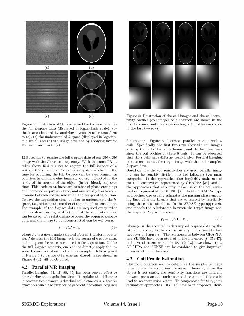
Figure 5: Illustration of the coil images and the coil sensi-tivity profiles (coil images of 8 channels are shown in thefirst two rows, and the corresponding coil profiles are shownin the last two rows).

for imaging. Figure 5 illustrates parallel imaging with 8coils. Specifically, the first two rows show the coil imagesseen by the individual coil/channel, and the last two rowsshow the coil profiles of these 8 coils. It can be observedthat the 8 coils have different sensitivities. Parallel imagingtries to reconstruct the target image with the undersampledk-space data.

Based on how the coil sensitivities are used, parallel imag-ing can be roughly divided into the following two maincategories: 1) the approaches that implicitly make use ofthe coil sensitivities, represented by GRAPPA [34], and 2)the approaches that explicitly make use of the coil sensi-tivities, represented by SENSE [88]. In the GRAPPA typeapproaches, one usually estimates the missing phase encod-ing lines with the kernels that are estimated by implicitlyusing the coil sensitivities. In the SENSE type approach,one models the relationship between the target image andthe acquired k-space data as:

yi = FuSif + ni, (20)

where yi is the acquired undersampled k-space data by thei-th coil, and Si is the coil sensitivity maps (see the lasttwo rows of Figure 5). The relationships between GRAPPAand SENSE have been studied in the literature [8; 35; 47],and several recent work [57; 58; 72; 73] have shown thatGRAPPA and SENSE can be combined to give improvedreconstruction performance.

4.3 Coil Profile EstimationThe most common way to determine the sensitivity mapsis to obtain low-resolution pre-scans. However, when theobject is not static, the sensitivity functions are differentbetween pre-scan and under-sampled scans, and this couldlead to reconstruction errors. To compensate for this, jointestimation approaches [103; 113] have been proposed. How-


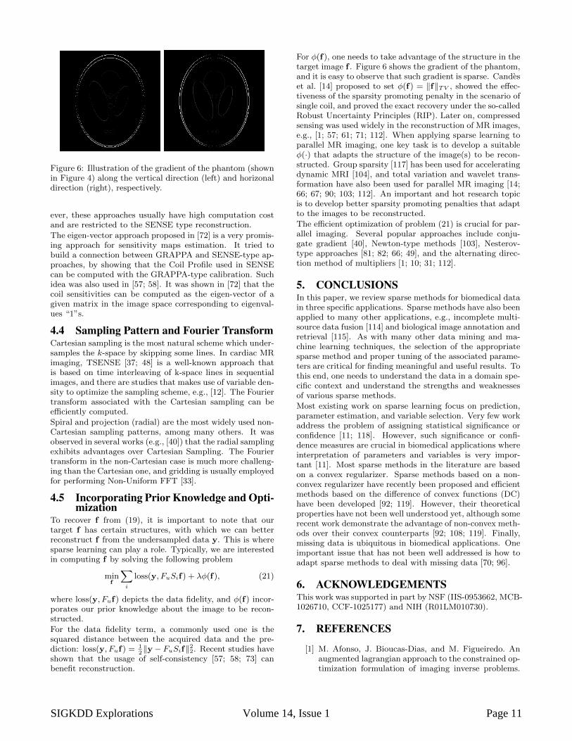
Figure 6: Illustration of the gradient of the phantom (shownin Figure 4) along the vertical direction (left) and horizonaldirection (right), respectively.

ever, these approaches usually have high computation costand are restricted to the SENSE type reconstruction.

The eigen-vector approach proposed in [72] is a very promis-ing approach for sensitivity maps estimation. It tried tobuild a connection between GRAPPA and SENSE-type ap-proaches, by showing that the Coil Profile used in SENSEcan be computed with the GRAPPA-type calibration. Suchidea was also used in [57; 58]. It was shown in [72] that thecoil sensitivities can be computed as the eigen-vector of agiven matrix in the image space corresponding to eigenval-ues “1”s.

4.4 Sampling Pattern and Fourier TransformCartesian sampling is the most natural scheme which under-samples the k-space by skipping some lines. In cardiac MRimaging, TSENSE [37; 48] is a well-known approach thatis based on time interleaving of k-space lines in sequentialimages, and there are studies that makes use of variable den-sity to optimize the sampling scheme, e.g., [12]. The Fouriertransform associated with the Cartesian sampling can beefficiently computed.

Spiral and projection (radial) are the most widely used non-Cartesian sampling patterns, among many others. It wasobserved in several works (e.g., [40]) that the radial samplingexhibits advantages over Cartesian Sampling. The Fouriertransform in the non-Cartesian case is much more challeng-ing than the Cartesian one, and gridding is usually employedfor performing Non-Uniform FFT [33].

4.5 Incorporating Prior Knowledge and Opti-mization

To recover f from (19), it is important to note that ourtarget f has certain structures, with which we can betterreconstruct f from the undersampled data y. This is wheresparse learning can play a role. Typically, we are interestedin computing f by solving the following problem

minf

∑i

loss(y, FuSif) + λφ(f), (21)

where loss(y, Fuf) depicts the data fidelity, and φ(f) incor-porates our prior knowledge about the image to be recon-structed.

For the data fidelity term, a commonly used one is thesquared distance between the acquired data and the pre-diction: loss(y, Fuf) = 1

2‖y− FuSif‖22. Recent studies have

shown that the usage of self-consistency [57; 58; 73] canbenefit reconstruction.

For φ(f), one needs to take advantage of the structure in thetarget image f . Figure 6 shows the gradient of the phantom,and it is easy to observe that such gradient is sparse. Candeset al. [14] proposed to set φ(f) = ‖f‖TV , showed the effec-tiveness of the sparsity promoting penalty in the scenario ofsingle coil, and proved the exact recovery under the so-calledRobust Uncertainty Principles (RIP). Later on, compressedsensing was used widely in the reconstruction of MR images,e.g., [1; 57; 61; 71; 112]. When applying sparse learning toparallel MR imaging, one key task is to develop a suitableφ(·) that adapts the structure of the image(s) to be recon-structed. Group sparsity [117] has been used for acceleratingdynamic MRI [104], and total variation and wavelet trans-formation have also been used for parallel MR imaging [14;66; 67; 90; 103; 112]. An important and hot research topicis to develop better sparsity promoting penalties that adaptto the images to be reconstructed.

The efficient optimization of problem (21) is crucial for par-allel imaging. Several popular approaches include conju-gate gradient [40], Newton-type methods [103], Nesterov-type approaches [81; 82; 66; 49], and the alternating direc-tion method of multipliers [1; 10; 31; 112].

5. CONCLUSIONSIn this paper, we review sparse methods for biomedical datain three specific applications. Sparse methods have also beenapplied to many other applications, e.g., incomplete multi-source data fusion [114] and biological image annotation andretrieval [115]. As with many other data mining and ma-chine learning techniques, the selection of the appropriatesparse method and proper tuning of the associated parame-ters are critical for finding meaningful and useful results. Tothis end, one needs to understand the data in a domain spe-cific context and understand the strengths and weaknessesof various sparse methods.

Most existing work on sparse learning focus on prediction,parameter estimation, and variable selection. Very few workaddress the problem of assigning statistical significance orconfidence [11; 118]. However, such significance or confi-dence measures are crucial in biomedical applications whereinterpretation of parameters and variables is very impor-tant [11]. Most sparse methods in the literature are basedon a convex regularizer. Sparse methods based on a non-convex regularizer have recently been proposed and efficientmethods based on the difference of convex functions (DC)have been developed [92; 119]. However, their theoreticalproperties have not been well understood yet, although somerecent work demonstrate the advantage of non-convex meth-ods over their convex counterparts [92; 108; 119]. Finally,missing data is ubiquitous in biomedical applications. Oneimportant issue that has not been well addressed is how toadapt sparse methods to deal with missing data [70; 96].

6. ACKNOWLEDGEMENTSThis work was supported in part by NSF (IIS-0953662, MCB-1026710, CCF-1025177) and NIH (R01LM010730).

7. REFERENCES

[1] M. Afonso, J. Bioucas-Dias, and M. Figueiredo. Anaugmented lagrangian approach to the constrained op-timization formulation of imaging inverse problems.


IEEE Transactions on Image Processing, 20:681–695,2011.

[2] A. Argyriou, T. Evgeniou, and M. Pontil. Con-vex multi-task feature learning. Machine Learning,73(3):243–272, 2008.

[3] F. R. Bach. Consistency of the group lasso and multi-ple kernel learning. Journal of Machine Learning Re-search, 9:1179–1225, 2008.

[4] W. Bajwa, J. Haupt, A. Sayeed, and R. Nowak. Com-pressive wireless sensing. In International Conferenceon Information Processing in Sensor Networks, 2006.

[5] O. Banerjee, L. El Ghaoui, and A. d’Aspremont.Model selection through sparse maximum likelihoodestimation for multivariate gaussian or binary data.The Journal of Machine Learning Research, 9:485–516, 2008.

[6] R. Baraniuk. Compressive sensing. IEEE Signal Pro-cessing Magazine, 24(4):118–121, 2007.

[7] M. Belkin and P. Niyogi. Laplacian eigenmaps for di-mensionality reduction and data representation. Neu-ral Computation, 15:1373–1396, 2003.

[8] M. Blaimer, F. Breuer, M. Muller, R. Heidemann,M. A. Griswold, and P. M. Jakob. SMASH, SENSE,PILS, GRAPPA. Top Magn Reson Imaging, 15:223–236, 2004.

[9] H. Bondell and B. Reich. Simultaneous regressionshrinkage, variable selection, and supervised cluster-ing of predictors with oscar. Biometrics, 64(1):115–123, 2008.

[10] S. Boyd, N. Parikh, E. Chu, B. Peleato, and J. Eck-stein. Distributed optimization and statistical learningvia the alternating direction method of multipliers.Foundations and Trends in Machine Learning, 3:1–122, 2011.

[11] P. Buhlmann. Statistical significance in high-dimensional linear models. Arxiv preprintarXiv:1202.1377v1, 2012.

[12] R. Busse, K. Wang, J. Holmes, J. Brittain, and F. Ko-rosec. Optimization of variable-density cartesian sam-pling for time-resolved imaging. In International Soci-ety for Magnetic Resonance in Medicine, 2009.

[13] E. Candes and J. Romberg. Quantitative robust un-certainty principles and optimally sparse decompo-sitions. Foundations of Computational Mathematics,6(2):227–254, 2006.

[14] E. Candes, J. Romberg, and T. Tao. Robust uncer-tainty principles: Exact signal reconstruction fromhighly incomplete frequency information. IEEE Trans-actions on Information Theory, 52(2):489–509, 2006.

[15] E. Candes and T. Tao. Near optimal signal recoveryfrom random projections: Universal encoding strate-gies? IEEE Transactions on Information Theory,52(12):5406–5425, 2006.

[16] E. Candes and M. Wakin. An introduction to com-pressive sampling. IEEE Signal Processing Magazine,25(2):21–30, 2008.

[17] S. Carroll, J. Grenier, and S. Weatherbee. From DNAto Diversity: Molecular Genetics and the Evolution ofAnimal Design. 2nd edition. Malden, MA: BlackwellPub, 2005.

[18] W. Chu, Z. Ghahramani, F. Falciani, and D. Wild.Biomarker discovery in microarray gene expres-sion data with gaussian processes. Bioinformatics,21(16):3385–3393, 2005.

[19] H. Chuang, E. Lee, Y. Liu, D. Lee, and T. Ideker.Network-based classification of breast cancer metasta-sis. Molecular systems biology, 3:140, 2007.

[20] F. Chung. Spectral Graph Theory. American Mathe-matical Society, 1997.

[21] D. Cox. Regression models and life-tables. Journal ofthe Royal Statistical Society. Series B (Methodologi-cal), 34(2):187–220, 1972.

[22] P. Danaher, P. Wang, and D. Daniela. The joint graph-ical lasso for inverse covariance estimation across mul-tiple classes. Arxiv preprint arXiv:1111.0324, 2011.

[23] A. d’Aspremont, L. El Ghaoui, M. Jordan, andG. R. G. Lanckriet. A direct formulation for sparsePCA using semidefinite programming. In NIPS, 2005.

[24] D. Donoho. High-dimensional data analysis: Thecurses and blessings of dimensionality. 2000.

[25] D. Donoho. Compressed sensing. IEEE Transactionson Information Theory, 52:1289–1306, 2006.

[26] M. Duarte, M. Davenport, M. Wakin, and R. Bara-niuk. Sparse signal detection from incoherent projec-tions. In ICASSP, 2006.

[27] J. Fan and J. Lv. A selective overview of variable se-lection in high dimensional feature space. StatisticaSinica, 20:101–148, 2010.

[28] J. Friedman, T. Hastie, H. Hofling, and R. Tibshirani.Pathwise coordinate optimization. Annals of AppliedStatistics, 1(2):302–332, 2007.

[29] J. Friedman, T. Hastie, and R. Tibshirani. Sparse in-verse covariance estimation with the graphical lasso.Biostatistics, 9(3):432–441, 2008.

[30] J. Friedman, T. Hastie, and R. Tibshirani. A note onthe group lasso and a sparse group lasso. Technicalreport, Department of Statistics, Stanford University,2010.

[31] T. Goldstein and S. Osher. The split bregman methodfor l1-regularized problems. SIAM Journal on ImagingSciences, 2:323–343, 2009.

[32] T. R. Golub, D. K. Slonim, P. Tamayo, C. Huard,M. Gaasenbeek, J. P. Mesirov, H. Coller, M. L. Loh,J. R. Downing, M. A. Caligiuri, and C. D. Bloomfield.Molecular classification of cancer: Class discovery andclass prediction by gene expression monitoring. Sci-ence, 286(5439):531–537, 1999.


[33] L. Greengard and J. Lee. Accelerating the nonuni-form fast fourier transform. SIAM Review, 46:443–454,2004.

[34] M. A. Griswold, P. M. Jakob, R. M. Heidemann,M. Nittka, V. Jellus, J. Wang, K. B., and A. Haase.Generalized autocalibrating partially parallel acquisi-tions (GRAPPA). Magnetic Resonance in Medicine,47:1202–1210, 2002.

[35] M. A. Griswold, S. Kannengiesser, R. M. Heidemann,J. Wang, and P. M. Jakob. Field-of-view limitationsin parallel imaging. Magnetic Resonance in Medicine,52:1118–1126, 2004.

[36] J. Guo, E. Levina, G. Michailidis, and J. Zhu. Jointestimation of multiple graphical models. Biometrika,98(1):1–15, 2011.

[37] M. A. Guttman, P. Kellman, A. J. Dick, R. J. Led-erman, and E. R. McVeigh. Real-time accelerated in-teractive MRI with adaptive TSENSE and UNFOLD.Magnetic Resonance in Medicine, 50:315–321, 2003.

[38] I. Guyon, J. Weston, S. Barnhill, and V. Vapnik. Geneselection for cancer classification using support vectormachines. Machine Learning, 46(1-3):389–422, 2002.

[39] E. M. Haacke, R. W. Brown, M. R. Thompson, andR. Venkatesan, editors. Magnetic Resonance Imaging:Physical Principles and Sequence Design. Wiley-Liss,1999.

[40] M. S. Hansen, C. Baltes, J. Tsao, S. Kozerke, K. P.Pruessmann, and H. Eggers. k-t BLAST reconstruc-tion from non-cartesian k-t space sampling. MagneticResonance in Medicine, 55:85–91, 2006.

[41] T. Hromadka, M. DeWeese, and A. Zador. Sparse rep-resentation of sounds in the unanesthetized auditorycortex. PLoS Biol, 6(1):e16, 2008.

[42] J. Huang, T. Zhang, and D. Metaxas. Learning withstructured sparsity. Journal of Machine Learning Re-search, 12:3371–3412, 2011.

[43] S. Huang, J. Li, L. Sun, J. Liu, T. Wu, K. Chen,A. Fleisher, E. Reiman, and J. Ye. Learning brainconnectivity of alzheimer’s disease from neuroimagingdata. In NIPS, pages 808–816, 2009.

[44] L. Jacob, G. Obozinski, and J. Vert. Group lasso withoverlap and graph lasso. In ICML, 2009.

[45] R. Jenatton, J.-Y. Audibert, and F. Bach. Struc-tured variable selection with sparsity-inducing norms.Journal of Machine Learning Research, 12:2777–2824,2011.

[46] R. Jenatton, J. Mairal, G. Obozinski, and F. Bach.Proximal methods for sparse hierarchical dictionarylearning. In ICML, 2010.

[47] P. Kellman. Parallel imaging: the basics. In ISMRMEducational Course: MR Physics for Physicists, 2004.

[48] P. Kellman, F. H. Epstein, and E. R. McVeigh. Adap-tive sensitivity encoding incorporating temporal filter-ing (tsense). Magnetic Resonance in Medicine, 45:846–852, 2001.

[49] K. Khare, C. J. Hardy, K. F. King, P. A. Turski, andL. Marinelli. Accelerated MR imaging using compres-sive sensing with no free parameters. Magnetic Reso-nance in Medicine, 2012.

[50] S. Kim and E. Xing. Statistical estimation of corre-lated genome associations to a quantitative trait net-work. PLoS genetics, 5(8):e1000587, 2009.

[51] S. Kim and E. P. Xing. Tree-guided group lassofor multi-task regression with structured sparsity. InICML, 2010.

[52] K. Koh, S. Kim, and S. Boyd. An interior-pointmethod for large-scale l1-regularized logistic regres-sion. Journal of Machine Learning Research, 8:1519–1555, 2007.

[53] M. Kolar, L. Song, A. Ahmed, and E. Xing. Esti-mating time-varying networks. The Annals of AppliedStatistics, 4(1):94–123, 2010.

[54] M. Kolar and E. Xing. On time varying undirectedgraphs. In AISTAT, 2011.

[55] M. Kowalski. Sparse regression using mixed norms.Applied and Computational Harmonic Analysis,27(3):303–324, 2009.

[56] S. Kumar, K. Jayaraman, S. Panchanathan, R. Gu-runathan, A. Marti-Subirana, and S. Newfeld. BEST:A novel computational approach for comparing geneexpression patterns from early stages of Drosophilamelanogaster development. Genetics, 162(4):2037–2047, 2002.

[57] P. Lai, M. Lustig, B. A. C., V. S. S., B. P. J., andA. M. Efficient L1SPIRiT reconstruction (ESPIRiT)for highly accelerated 3d volumetric MRI with parallelimaging and compressed sensing. In ISMRM, 2010.

[58] P. Lai, M. Lustig, V. S. S., and B. A. C. ESPIRiT (effi-cient eigenvector-based l1spirit) for compressed sens-ing parallel imaging - theoretical interpretation andimproved robustness for overlapped FOV prescription.In ISMRM, 2011.

[59] D. J. Larkman and R. G. Nunes. Parallel magneticresonance imaging. Physics in Medicine and Biology,52:R15–55, 2007.

[60] C. Li and H. Li. Network-constrained regularizationand variable selection for analysis of genomic data.Bioinformatics, 24(9):1175–1182, 2008.

[61] D. Liang, B. Liu, J. Wang, and L. Ying. Accelerat-ing SENSE using compressed sensing. Magnetic Reso-nance in Medicine, 62:1574–1584, 2009.

[62] H. Liu, M. Palatucci, and J. Zhang. Blockwise co-ordinate descent procedures for the multi-task lasso,with applications to neural semantic basis discovery.In ICML, 2009.


[63] H. Liu, K. Roeder, and L. Wasserman. Stability ap-proach to regularization selection (StARS) for high di-mensional graphical models. In NIPS, 2011.

[64] J. Liu, S. Ji, and J. Ye. Multi-task feature learning viaefficient `2,1-norm minimization. In UAI, 2009.

[65] J. Liu, S. Ji, and J. Ye. SLEP: Sparse Learning withEfficient Projections. Arizona State University, 2009.

[66] J. Liu, J. Rapin, T. Chang, A. Lefebvre, M. Zenge,E. Mueller, and M. S. Nadar. Dynamic cardiac MRI re-construction with weighted redundant haar wavelets.In ISMRM, 2012.

[67] J. Liu, J. Rapin, T. Chang, P. Schmitt, X. Bi,A. Lefebvre, M. Zenge, E. Mueller, and M. S.Nadar. Regularized reconstruction using redundanthaar wavelets: A means to achieve high under-sampling factors in non-contrast-enhanced 4D MRA.In ISMRM, 2012.

[68] J. Liu and J. Ye. Efficient `1/`q norm regularization.Arxiv preprint arXiv:1009.4766v1, 2010.

[69] J. Liu and J. Ye. Moreau-Yosida regularization forgrouped tree structure learning. In NIPS, 2010.

[70] P. Loh and M. Wainwright. High-dimension regressionwith noisy and missing data: Provable guarantees withnon-convexity. In NIPS, 2011.

[71] M. Lustig, D. L. Donoho, and J. M. Pauly. SparseMRI: The application of compressed sensing forrapid MR imaging. Magnetic Resonance in Medicine,58:1182–1195, 2007.

[72] M. Lustig, P. Lai, M. Murphy, S. Vasanawala, M. Elad,J. Zhang, and J. Pauly. An eigen-vector approachto autocalibrating parallel MRI, where SENSE meetsGRAPPA. In ISMRM, 2011.

[73] M. Lustig and J. M. Pauly. SPIRiT: Iterative self-consistent parallel imaging reconstruction from ar-bitrary k-space. Magnetic Resonance in Medicine,64:457–471, 2010.

[74] M. Marton et al. Drug target validation and identi-fication of secondary drug target effects using DNAmicroarrays. Nature Medicine, 4(11):1293–1301, 1998.

[75] R. Mazumder and T. Hastie. Exact covariance thresh-olding into connected components for large-scalegraphical lasso. Arxiv preprint arXiv:1108.3829, 2011.

[76] R. Mazumder and T. Hastie. The graphical lasso:New insights and alternatives. Arxiv preprintarXiv:1111.5479, 2011.

[77] S. Megason and S. Fraser. Imaging in systems biology.Cell, 130(5):784–795, 2007.

[78] L. Meier, S. Geer, and P. Buhlmann. The group lassofor logistic regression. Journal of the Royal StatisticalSociety: Series B, 70:53–71, 2008.

[79] N. Meinshausen and P. Buhlmann. Stability selection.Journal of the Royal Statistical Society: Series B,72:417–473, 2010.

[80] S. Negahban and M. Wainwright. Joint support recov-ery under high-dimensional scaling: Benefits and per-ils of `1,∞-regularization. In NIPS, pages 1161–1168.2008.

[81] A. Nemirovski. Efficient methods in convex program-ming. Lecture Notes, 1994.

[82] Y. Nesterov. Introductory Lectures on Convex Opti-mization: A Basic Course. Kluwer Academic Publish-ers, 2004.

[83] Y. Nesterov. Gradient methods for minimizing com-posite objective function. CORE, 2007.

[84] A. Ng. Feature selection, `1 vs. `2 regularization, androtational invariance. In ICML, 2004.

[85] G. Obozinski, B. Taskar, and M. I. Jordan. Joint co-variate selection for grouped classification. Technicalreport, Statistics Department, UC Berkeley, 2007.

[86] H. Peng. Bioimage informatics: a new area of engineer-ing biology. Bioinformatics, 24(17):1827–1836, 2008.

[87] J. Peng, J. Zhu, B. A., W. Han, D.-Y. Noh, J. R. Pol-lack, and P. Wang. Regularized multivariate regres-sion for identifying master predictors with applicationto integrative genomics study of breast cancer. Annalsof Applied Statistics, 4(1):53–77, 2010.

[88] K. Pruessmann, M. Weiger, M. Scheidegger, andP. Boesiger. SENSE: sensitivity endcoding for fastMRI. Magnetic Resonance in Medicine, 42:952–962,1999.

[89] A. Quattoni, X. Carreras, M. Collins, and T. Dar-rell. An efficient projection for `1,∞ regularization. InICML, 2009.

[90] S. Ramani and J. A. Fessler. Parallel MR image recon-struction using augmented lagrangian methods. IEEETransactions on Medical Imaging, 30:694–706, 2011.

[91] S. Ryali, K. Supekar, D. Abrams, and V. Menon.Sparse logistic regression for whole-brain classificationof fMRI data. Neuroimage, 51(2):752–764, 2010.

[92] X. Shen, W. Pan, and Y. Zhu. Likelihood-based se-lection and sharp parameter estimation. Journal ofAmerican Statistical Association, 107:223–232, 2012.

[93] J. Shi, W. Yin, S. Osher, and P. Sajda. A fast algo-rithm for large scale `1-regularized logistic regression.Technical report, CAAM TR08-07, 2008.

[94] W. Shi, K. Lee, and G. Wahba. Detecting disease-causing genes by lasso-patternsearch algorithm. BMCProceedings, 1(Suppl 1):S60, 2007.

[95] D. Sodickson and W. Manning. Simultaneous acqui-sition of spatial harmonics (SMASH): fast imagingwith radiofrequency coil arrays. Magnetic Resonancein Medicine, 38:591–603, 1997.

[96] N. Stadler and P. Buhlmann. Missing values: sparseinverse covariance estimation and an extension tosparse regression. Statistics and Computing, 22:219–235, 2012.


[97] A. Subramanian et al. Gene set enrichment analysis:a knowledge-based approach for interpreting genome-wide expression profiles. Proceedings of the NationalAcademy of Sciences of the United States of America,102(43):15545–15550, 2005.

[98] R. Tibshirani. Regression shrinkage and selection viathe lasso. Journal of the Royal Statistical Society Se-ries B, 58(1):267–288, 1996.

[99] R. Tibshirani, M. Saunders, S. Rosset, J. Zhu, andK. Knight. Sparsity and smoothness via the fusedlasso. Journal Of The Royal Statistical Society SeriesB, 67(1):91–108, 2005.

[100] R. Tibshirani and P. Wang. Spatial smoothing andhot spot detection for cgh data using the fused lasso.Biostatistics, 9(1):18–29, 2008.

[101] P. Tomancak, A. Beaton, R. Weiszmann, E. Kwan,S. Shu, S. E. Lewis, S. Richards, M. Ashburner,V. Hartenstein, S. E. Celniker, and G. M. Rubin.Systematic determination of patterns of gene expres-sion during Drosophila embryogenesis. Genome Biol-ogy, 3(12):research0088.1–14, 2002.

[102] A. Tropp, A. Gilbert, and M. Strauss. Algorithms forsimultaneous sparse approximation: part I: Greedypursuit. Signal Processing, 86(3):572–588, 2006.

[103] M. Uecker, T. Hohage, K. T. Block, and J. Frahm. Im-age reconstruction by regularized nonlinear inversion -joint estimation of coil sensitivities and image content.Magnetic Resonance in Medicine, 60:674–682, 2008.

[104] M. Usman, C. Prieto, T. Schaeffter, and P. G.Batchelor. k-t group sparse: A method for accelerat-ing dynamic MRI. Magnetic Resonance in Medicine,66:1163–1176, 2011.

[105] M. T. Vlaardingerbroek and J. A. Boer, editors. Mag-netic Resonance Imaging. Spinger, 2004.

[106] D. Witten, J. Friedman, and N. Simon. New in-sights and faster computations for the graphical lasso.Journal of Computational and Graphical Statistics,20(4):892–900, 2011.

[107] T. Wu, Y. Chen, T. Hastie, E. Sobel, and K. Lange.Genome-wide association analysis by lasso penal-ized logistic regression. Bioinformatics, 25(6):714–721,2009.

[108] S. Xiang, X. Shen, and J. Ye. Efficient sparse groupfeature selection via nonconvex optimization. Arxivpreprint arXiv:1205.5075, 2012.

[109] S. Yang, Z. Pan, X. Shen, P. Wonka, and J. Ye. Fusedmultiple graphical lasso. Technical Report, ArizonaState University, 2012.

[110] S. Yang, L. Yuan, Y.-C. Lai, X. Shen, P. Wonka, andJ. Ye. Feature grouping and selection over an undi-rected graph. In KDD, 2012.

[111] J. Ye, M. Farnum, E. Yang, R. Verbeeck, V. Lobanov,N. Raghavan, G. Novak, A. DiBernardo, andV. Narayan. Sparse learning and stability selection forpredicting MCI to AD conversion using baseline ADNIdata. BMC Neurology, 2012.

[112] X. Ye, Y. Chen, and F. Huang. Computational accel-eration for MR image reconstruction in partially par-allel imaging. IEEE Transactions on Medical Imaging,30:1055–1063, 2011.

[113] L. Ying and J. Sheng. Joint image reconstruction andsensitivity estimation in sense (JSENSE). MagneticResonance in Medicine, 57:1196–1202, 2007.

[114] L. Yuan, Y. Wang, P. Thompson, V. Narayand, andJ. Ye. Multi-source feature learning for joint analy-sis of incomplete multiple heterogeneous neuroimagingdata. NeuroImage, 61(3):622–632, 2012.

[115] L. Yuan, A. Woodard, S. Ji, Y. Jiang, Z.-H. Zhou,S. Kumar, and J. Ye. Learning sparse representationsfor fruit-fly gene expression pattern image annotationand retrieval. BMC Bioinformatics, 13:107, 2012.

[116] M. Yuan, V. R. Joseph, and H. Zou. Structuredvariable selection and estimation. Annals of AppliedStatistics, 3:1738–1757, 2009.

[117] M. Yuan and Y. Lin. Model selection and estimationin regression with grouped variables. Journal Of TheRoyal Statistical Society Series B, 68(1):49–67, 2006.

[118] C.-H. Zhang and S. Zhang. Confidence intervalsfor low-dimensional parameters with high-dimensionaldata. Arxiv preprint arXiv:1110.2563v1, 2011.

[119] T. Zhang. Analysis of multi-stage convex relaxationfor sparse regularization. Journal of Machine LearningResearch, 11:1081–1107, 2010.

[120] P. Zhao, G. Rocha, and B. Yu. The composite abso-lute penalties family for grouped and hierarchical vari-able selection. Annals of Statistics, 37(6A):3468–3497,2009.

[121] L. Zhong and J. Kwok. Efficient sparse modeling withautomatic feature grouping. ICML, 2011.

[122] S. Zhou, J. Lafferty, and L. Wasserman. Time varyingundirected graphs. COLT, 2008.

[123] J. Zhu and T. Hastie. Classification of gene microar-rays by penalized logistic regression. Biostatistics,5(3):427–443, 2004.

[124] J. Zhu, S. Rosset, T. Hastie, and R. Tibshirani. 1-norm support vector machines. In Neural InformationProcessing Systems, pages 49–56, 2003.

[125] Y. Zhu, X. Shen, and W. Pan. Simultaneous group-ing pursuit and feature selection in regression over anundirected graph. Preprint, 2012.

[126] H. Zou and T. Hastie. Regularization and variable se-lection via the elastic net. Journal of The Royal Sta-tistical Society Series B, 67(2):301–320, 2005.

[127] H. Zou, T. Hastie, and R. Tibshirani. Sparse princi-ple component analysis. Journal of Computational andGraphical Statistics, 15(2):262–286, 2006.


Documents

Sparse Methods for Biomedical Data