Embed Size (px)
Citation preview
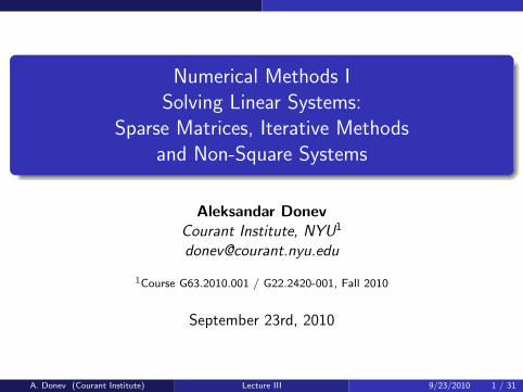
Numerical Methods ISolving Linear Systems:
Sparse Matrices, Iterative Methodsand Non-Square Systems
Aleksandar DonevCourant Institute, NYU1
1Course G63.2010.001 / G22.2420-001, Fall 2010
September 23rd, 2010
A. Donev (Courant Institute) Lecture III 9/23/2010 1 / 31
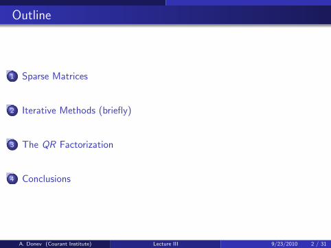
Outline
1 Sparse Matrices
2 Iterative Methods (briefly)
3 The QR Factorization
4 Conclusions
A. Donev (Courant Institute) Lecture III 9/23/2010 2 / 31
Sparse Matrices
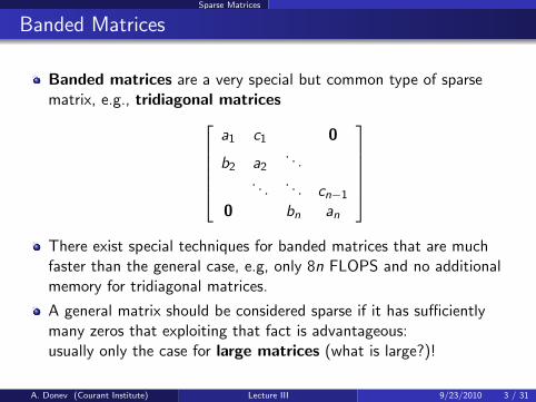
Banded Matrices
Banded matrices are a very special but common type of sparsematrix, e.g., tridiagonal matrices
a1 c1 0
b2 a2. . .
. . .. . . cn−1
0 bn an
There exist special techniques for banded matrices that are muchfaster than the general case, e.g, only 8n FLOPS and no additionalmemory for tridiagonal matrices.
A general matrix should be considered sparse if it has sufficientlymany zeros that exploiting that fact is advantageous:usually only the case for large matrices (what is large?)!
A. Donev (Courant Institute) Lecture III 9/23/2010 3 / 31
Sparse Matrices
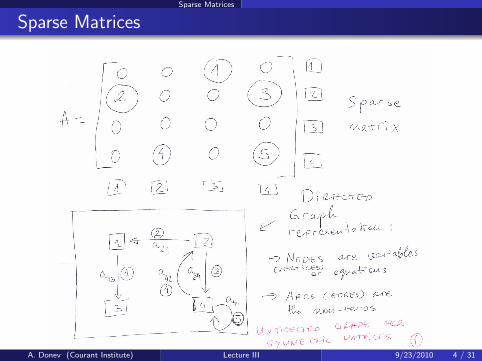
Sparse Matrices
A. Donev (Courant Institute) Lecture III 9/23/2010 4 / 31
Sparse Matrices
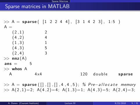
Sparse matrices in MATLAB
>> A = sparse ( [ 1 2 2 4 4 ] , [ 3 1 4 2 3 ] , 1 : 5 )A =
( 2 , 1 ) 2( 4 , 2 ) 4( 1 , 3 ) 1( 4 , 3 ) 5( 2 , 4 ) 3
>> nnz (A)ans = 5>> whos A
A 4 x4 120 d o u b l e sparse
>> A = sparse ( [ ] , [ ] , [ ] , 4 , 4 , 5 ) ; % Pre−a l l o c a t e memory>> A(2 ,1)=2 ; A(4 ,2 )=4 ; A(1 ,3 )=1; A(4 ,3)=5; A(2 ,4)=3;
A. Donev (Courant Institute) Lecture III 9/23/2010 5 / 31
Sparse Matrices
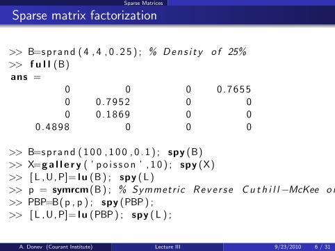
Sparse matrix factorization
>> B=s p r a n d ( 4 , 4 , 0 . 2 5 ) ; % Dens i t y o f 25%>> f u l l (B)ans =
0 0 0 0.76550 0 .7952 0 00 0 .1869 0 0
0 .4898 0 0 0
>> B=s p r a n d ( 1 0 0 , 1 0 0 , 0 . 1 ) ; spy (B)>> X=g a l l e r y ( ’ p o i s s o n ’ , 1 0 ) ; spy (X)>> [ L , U, P]= l u (B ) ; spy ( L )>> p = symrcm (B ) ; % Symmetric Reve r s e C u t h i l l−McKee o r d e r i n g>> PBP=B( p , p ) ; spy (PBP ) ;>> [ L , U, P]= l u (PBP ) ; spy ( L ) ;
A. Donev (Courant Institute) Lecture III 9/23/2010 6 / 31
Sparse Matrices
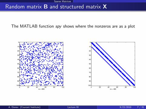
Random matrix B and structured matrix X
The MATLAB function spy shows where the nonzeros are as a plot
0 20 40 60 80 100
0
10
20
30
40
50
60
70
80
90
100
nz = 960
0 20 40 60 80 100
0
10
20
30
40
50
60
70
80
90
100
nz = 460
A. Donev (Courant Institute) Lecture III 9/23/2010 7 / 31
Sparse Matrices
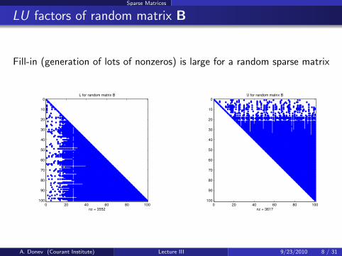
LU factors of random matrix B
Fill-in (generation of lots of nonzeros) is large for a random sparse matrix
0 20 40 60 80 100
0
10
20
30
40
50
60
70
80
90
100
nz = 3552
L for random matrix B
0 20 40 60 80 100
0
10
20
30
40
50
60
70
80
90
100
nz = 3617
U for random matrix B
A. Donev (Courant Institute) Lecture III 9/23/2010 8 / 31
Sparse Matrices
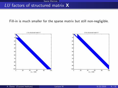
LU factors of structured matrix X
Fill-in is much smaller for the sparse matrix but still non-negligible.
0 20 40 60 80 100
0
10
20
30
40
50
60
70
80
90
100
nz = 1009
L for structured matrix X
0 20 40 60 80 100
0
10
20
30
40
50
60
70
80
90
100
nz = 1009
U for structured matrix X
A. Donev (Courant Institute) Lecture III 9/23/2010 9 / 31
Sparse Matrices
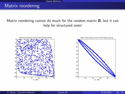
Matrix reordering
Matrix reordering cannot do much for the random matrix B, but it canhelp for structured ones!
0 20 40 60 80 100
0
10
20
30
40
50
60
70
80
90
100
nz = 960
Matrix B permuted by reverse Cuthill−McKee ordering
0 20 40 60 80 100
0
10
20
30
40
50
60
70
80
90
100
nz = 460
Matrix X permuted by reverse Cuthill−McKee ordering
A. Donev (Courant Institute) Lecture III 9/23/2010 10 / 31
Sparse Matrices
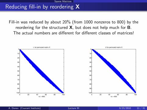
Reducing fill-in by reordering X
Fill-in was reduced by about 20% (from 1000 nonzeros to 800) by thereordering for the structured X, but does not help much for B.
The actual numbers are different for different classes of matrices!
0 20 40 60 80 100
0
10
20
30
40
50
60
70
80
90
100
nz = 805
L for permuted matrix X
0 20 40 60 80 100
0
10
20
30
40
50
60
70
80
90
100
nz = 805
U for permuted matrix X
A. Donev (Courant Institute) Lecture III 9/23/2010 11 / 31
Sparse Matrices
Importance of Sparse Matrix Structure
Important to remember: While there are general techniques fordealing with sparse matrices that help greatly, it all depends on thestructure (origin) of the matrix.
Pivoting has a dual, sometimes conflicting goal:
1 Reduce fill-in, i.e., improve memory use: Still active subject ofresearch!
2 Reduce roundoff error, i.e., improve stability. Typically somethreshold pivoting is used only when needed.
Pivoting for symmetric non-positive definite matrices is trickier:One can permute the diagonal entries only to preserve symmetry,but small diagonal entries require special treatment.
For many sparse matrices iterative methods (briefly covered nextlecture) are required to large fill-in.
A. Donev (Courant Institute) Lecture III 9/23/2010 12 / 31
Iterative Methods (briefly)
Why iterative methods?
Direct solvers are great for dense matrices and can be made to avoidroundoff errors to a large degree. They can also be implemented verywell on modern machines.
Fill-in is a major problem for certain sparse matrices and leads toextreme memory requirements (e.g., three-d.
Some matrices appearing in practice are too large to even berepresented explicitly (e.g., the Google matrix).
Often linear systems only need to be solved approximately, forexample, the linear system itself may be a linear approximation to anonlinear problem.
Direct solvers are much harder to implement and use on (massively)parallel computers.
A. Donev (Courant Institute) Lecture III 9/23/2010 13 / 31
Iterative Methods (briefly)
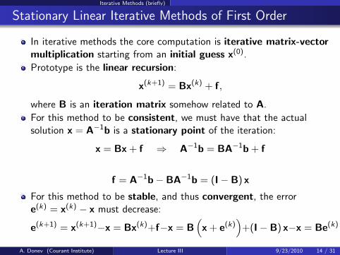
Stationary Linear Iterative Methods of First Order
In iterative methods the core computation is iterative matrix-vectormultiplication starting from an initial guess x(0).
Prototype is the linear recursion:
x(k+1) = Bx(k) + f,
where B is an iteration matrix somehow related to A.
For this method to be consistent, we must have that the actualsolution x = A−1b is a stationary point of the iteration:
x = Bx + f ⇒ A−1b = BA−1b + f
f = A−1b− BA−1b = (I− B) x
For this method to be stable, and thus convergent, the errore(k) = x(k) − x must decrease:
e(k+1) = x(k+1)−x = Bx(k)+f−x = B(
x + e(k))
+(I− B) x−x = Be(k)
A. Donev (Courant Institute) Lecture III 9/23/2010 14 / 31
Iterative Methods (briefly)
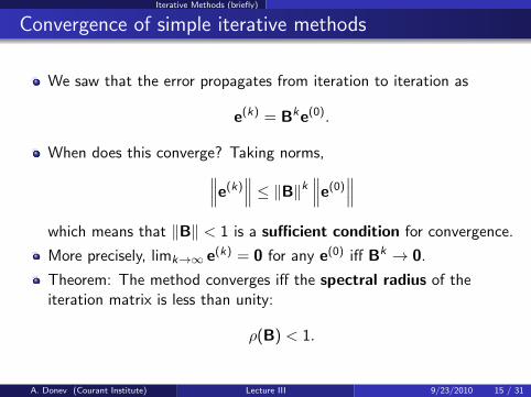
Convergence of simple iterative methods
We saw that the error propagates from iteration to iteration as
e(k) = Bke(0).
When does this converge? Taking norms,∥∥∥e(k)∥∥∥ ≤ ‖B‖k ∥∥∥e(0)
∥∥∥which means that ‖B‖ < 1 is a sufficient condition for convergence.
More precisely, limk→∞ e(k) = 0 for any e(0) iff Bk → 0.
Theorem: The method converges iff the spectral radius of theiteration matrix is less than unity:
ρ(B) < 1.
A. Donev (Courant Institute) Lecture III 9/23/2010 15 / 31
Iterative Methods (briefly)
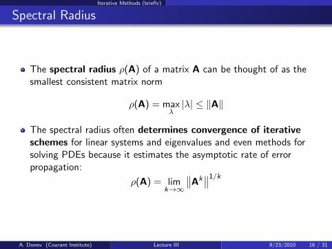
Spectral Radius
The spectral radius ρ(A) of a matrix A can be thought of as thesmallest consistent matrix norm
ρ(A) = maxλ|λ| ≤ ‖A‖
The spectral radius often determines convergence of iterativeschemes for linear systems and eigenvalues and even methods forsolving PDEs because it estimates the asymptotic rate of errorpropagation:
ρ(A) = limk→∞
∥∥Ak∥∥1/k
A. Donev (Courant Institute) Lecture III 9/23/2010 16 / 31
Iterative Methods (briefly)
Termination
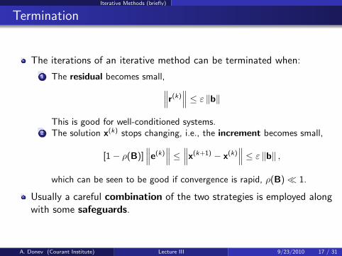
The iterations of an iterative method can be terminated when:
1 The residual becomes small,∥∥∥r(k)∥∥∥ ≤ ε ‖b‖
This is good for well-conditioned systems.2 The solution x(k) stops changing, i.e., the increment becomes small,
[1− ρ(B)]∥∥∥e(k)
∥∥∥ ≤ ∥∥∥x(k+1) − x(k)∥∥∥ ≤ ε ‖b‖ ,
which can be seen to be good if convergence is rapid, ρ(B)� 1.
Usually a careful combination of the two strategies is employed alongwith some safeguards.
A. Donev (Courant Institute) Lecture III 9/23/2010 17 / 31
Iterative Methods (briefly)
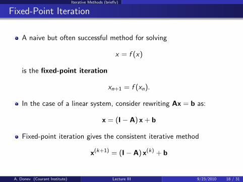
Fixed-Point Iteration
A naive but often successful method for solving
x = f (x)
is the fixed-point iteration
xn+1 = f (xn).
In the case of a linear system, consider rewriting Ax = b as:
x = (I− A) x + b
Fixed-point iteration gives the consistent iterative method
x(k+1) = (I− A) x(k) + b
A. Donev (Courant Institute) Lecture III 9/23/2010 18 / 31
Iterative Methods (briefly)
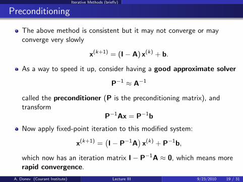
Preconditioning
The above method is consistent but it may not converge or mayconverge very slowly
x(k+1) = (I− A) x(k) + b.
As a way to speed it up, consider having a good approximate solver
P−1 ≈ A−1
called the preconditioner (P is the preconditioning matrix), andtransform
P−1Ax = P−1b
Now apply fixed-point iteration to this modified system:
x(k+1) =(I− P−1A
)x(k) + P−1b,
which now has an iteration matrix I− P−1A ≈ 0, which means morerapid convergence.
A. Donev (Courant Institute) Lecture III 9/23/2010 19 / 31
Iterative Methods (briefly)
Preconditioned Iteration
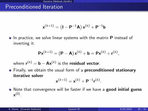
x(k+1) =(I− P−1A
)x(k) + P−1b
In practice, we solve linear systems with the matrix P instead ofinverting it:
Px(k+1) = (P− A) x(k) + b = Px(k) + r(k),
where r(k) = b− Ax(k) is the residual vector.
Finally, we obtain the usual form of a preconditioned stationaryiterative solver
x(k+1) = x(k) + P−1r(k).
Note that convergence will be faster if we have a good initial guessx(0).
A. Donev (Courant Institute) Lecture III 9/23/2010 20 / 31
Iterative Methods (briefly)
Some Standard Examples
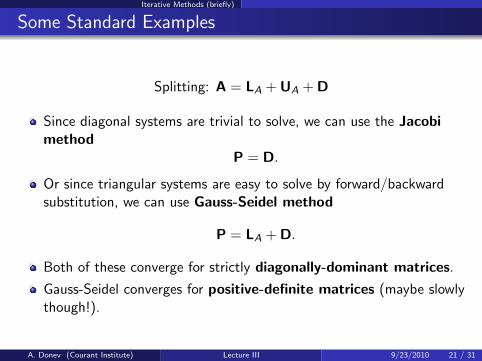
Splitting: A = LA + UA + D
Since diagonal systems are trivial to solve, we can use the Jacobimethod
P = D.
Or since triangular systems are easy to solve by forward/backwardsubstitution, we can use Gauss-Seidel method
P = LA + D.
Both of these converge for strictly diagonally-dominant matrices.
Gauss-Seidel converges for positive-definite matrices (maybe slowlythough!).
A. Donev (Courant Institute) Lecture III 9/23/2010 21 / 31
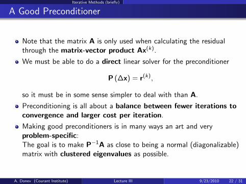
Iterative Methods (briefly)
A Good Preconditioner
Note that the matrix A is only used when calculating the residualthrough the matrix-vector product Ax(k).
We must be able to do a direct linear solver for the preconditioner
P (∆x) = r(k),
so it must be in some sense simpler to deal with than A.
Preconditioning is all about a balance between fewer iterations toconvergence and larger cost per iteration.
Making good preconditioners is in many ways an art and veryproblem-specific:The goal is to make P−1A as close to being a normal (diagonalizable)matrix with clustered eigenvalues as possible.
A. Donev (Courant Institute) Lecture III 9/23/2010 22 / 31
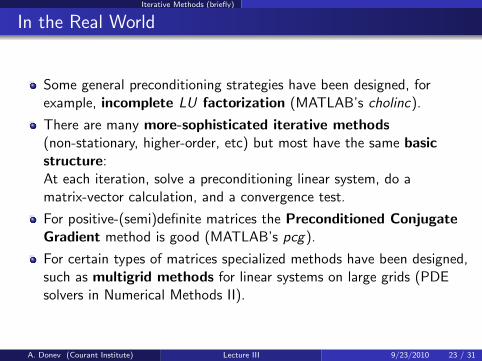
Iterative Methods (briefly)
In the Real World
Some general preconditioning strategies have been designed, forexample, incomplete LU factorization (MATLAB’s cholinc).
There are many more-sophisticated iterative methods(non-stationary, higher-order, etc) but most have the same basicstructure:At each iteration, solve a preconditioning linear system, do amatrix-vector calculation, and a convergence test.
For positive-(semi)definite matrices the Preconditioned ConjugateGradient method is good (MATLAB’s pcg).
For certain types of matrices specialized methods have been designed,such as multigrid methods for linear systems on large grids (PDEsolvers in Numerical Methods II).
A. Donev (Courant Institute) Lecture III 9/23/2010 23 / 31
The QR Factorization
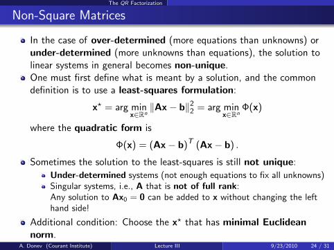
Non-Square Matrices
In the case of over-determined (more equations than unknowns) orunder-determined (more unknowns than equations), the solution tolinear systems in general becomes non-unique.One must first define what is meant by a solution, and the commondefinition is to use a least-squares formulation:
x? = arg minx∈Rn‖Ax− b‖2
2 = arg minx∈Rn
Φ(x)
where the quadratic form is
Φ(x) = (Ax− b)T (Ax− b) .
Sometimes the solution to the least-squares is still not unique:
Under-determined systems (not enough equations to fix all unknowns)Singular systems, i.e., A that is not of full rank:Any solution to Ax0 = 0 can be added to x without changing the lefthand side!
Additional condition: Choose the x? that has minimal Euclideannorm.
A. Donev (Courant Institute) Lecture III 9/23/2010 24 / 31
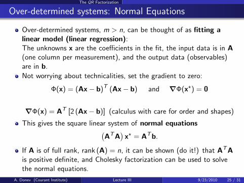
The QR Factorization
Over-determined systems: Normal Equations
Over-determined systems, m > n, can be thought of as fitting alinear model (linear regression):The unknowns x are the coefficients in the fit, the input data is in A(one column per measurement), and the output data (observables)are in b.
Not worrying about technicalities, set the gradient to zero:
Φ(x) = (Ax− b)T (Ax− b) and ∇Φ(x?) = 0
∇Φ(x) = AT [2 (Ax− b)] (calculus with care for order and shapes)
This gives the square linear system of normal equations(ATA
)x? = ATb.
If A is of full rank, rank (A) = n, it can be shown (do it!) that ATAis positive definite, and Cholesky factorization can be used to solvethe normal equations.
A. Donev (Courant Institute) Lecture III 9/23/2010 25 / 31
The QR Factorization
Problems with the normal equations
(ATA
)x? = ATb.
The conditioning number of the normal equations is
κ(ATA
)= [κ(A)]2
Furthermore, roundoff can cause ATA to no longer appear aspositive-definite and the Cholesky factorization will fail.
If the normal equations are ill-conditioned, another approach isneeded.
Also note that multiplying AT (n ×m) and A (m × n) takes n2
dot-products of length m, so O(mn2) operations, which can be muchlarger than O(n3) for the Cholesky factorization if m� n (fitting lotsof data with few parameters).
A. Donev (Courant Institute) Lecture III 9/23/2010 26 / 31
The QR Factorization
The QR factorization
For nonsquare or ill-conditioned matrices of full-rank r = n ≤ m, theLU factorization can be replaced by the QR factorization:
A =QR
[m × n] =[m × n][n × n]
where Q has orthogonal columns, QTQ = In, and R is anon-singular upper triangular matrix.
Observe that orthogonal / unitary matrices are well-conditioned(κ2 = 1), so the QR factorization is numerically better (but also moreexpensive!) than the LU factorization.
For matrices not of full rank there are modified QR factorizationsbut the SVD decomposition is better (next class).
In MATLAB, the QR factorization can be computed using qr (withcolumn pivoting).
A. Donev (Courant Institute) Lecture III 9/23/2010 27 / 31
The QR Factorization
Solving Linear Systems via QR factorization
(ATA
)x? = ATb where A = QR
Observe that R is the Cholesky factor of the matrix in the normalequations:
ATA = RT(QTQ
)R = RTR
(RTR
)x? =
(RTQT
)b ⇒ x? = R−1
(QTb
)which amounts to solving a triangular system with matrix R.This calculation turns out to be much more numerically stableagainst roundoff than forming the normal equations (and has similarcost).For under-determined full-rank systems, r = m ≤ n, one does a QRfactorization of AT = QR and the least-squares solution is
x? = Q(
R−T
b)
Practice: Derive the above formula and maybe prove least-squares.A. Donev (Courant Institute) Lecture III 9/23/2010 28 / 31
The QR Factorization
Computing the QR Factorization
Assume that
∃x s.t. b = Ax, that is,b ∈ range(A)
b = Q (Rx) = Qy ⇒ x = R−1y
showing that the columns of Q form an orthonormal basis for therange of A (linear subspace spanned by the columns of A).The QR factorization is thus closely-related to the orthogonalizationof a set of n vectors (columns) {a1, a2, . . . , an} in Rm.Classical approach is the Gram-Schmidt method: To make a vectorb orthogonal to a do:
b = b− (b · a)a
(a · a)
Practice: Verify that b · a = 0Repeat this in sequence: Start with a1 = a1, then make a2 orthogonalto a1, then make a3 orthogonal to a2 and a3.
A. Donev (Courant Institute) Lecture III 9/23/2010 29 / 31
The QR Factorization
Modified Gram-Schmidt Orthogonalization
More efficient formula (standard Gram-Schmidt):
ak+1 = ak+1 −k∑
j=1
(ak+1 · qj
)qj , qk+1 =
ak+1
‖ak+1‖,
with cost ∼ mn2 FLOPS.
A mathematically-equivalent but numerically much superior againstroundoff error is the modified Gram-Schmidt, in which eachorthogonalization is carried in sequence and repeated against eachof the already-computed basis vectors:Start with a1 = a1, then make a2 orthogonal to a1, then make a3
orthogonal to a2 and then make it orthogonal to a3.
The modified procedure is twice more expensive, ∼ 2mn2 FLOPS,but usually worth it.
Pivoting is strictly necessary for matrices not of full rank but it canalso improve stability in general.
A. Donev (Courant Institute) Lecture III 9/23/2010 30 / 31
Conclusions
Conclusions/Summary
Sparse matrices deserve special treatment but the details depend onthe specific field of application.
In particular, special sparse matrix reordering methods or iterativesystems are often required.
When sparse direct methods fail due to memory or otherrequirements, iterative methods are used instead.
Convergence of iterative methods depends strongly on the matrix, anda good preconditioner is often required.
There are good libraries for iterative methods as well (but youmust supply your own preconditioner!).
The QR factorization is a numerically-stable method for solvingfull-rank non-square systems.
For rank-defficient matrices the singular value decomposition (SVD)is best, discussed in later lectures.
A. Donev (Courant Institute) Lecture III 9/23/2010 31 / 31


![Solving Linear Systems: Iterative Methods and Sparse · PDF fileSolving Linear Systems: Iterative Methods and Sparse Systems ... [non-singular] matrix O(n3) LU decomposition Works](https://img.dokumen.tips/doc/110x75/5a7957ed7f8b9ac53b8d88c9/solving-linear-systems-iterative-methods-and-sparse-linear-systems-iterative.jpg)