Spacecraft Charging at Geosynchronous Altitudes: Current

Air Force Institute of Technology Air Force Institute of Technology

AFIT Scholar AFIT Scholar

Theses and Dissertations Student Graduate Works

3-3-2003

Spacecraft Charging at Geosynchronous Altitudes: Current Spacecraft Charging at Geosynchronous Altitudes: Current

Balance and Critical Temperature in a Non-Maxwellian Plasma Balance and Critical Temperature in a Non-Maxwellian Plasma

Jose T. Harris

Follow this and additional works at: https://scholar.afit.edu/etd

Part of the Plasma and Beam Physics Commons

Recommended Citation Recommended Citation Harris, Jose T., "Spacecraft Charging at Geosynchronous Altitudes: Current Balance and Critical Temperature in a Non-Maxwellian Plasma" (2003). Theses and Dissertations. 4166. https://scholar.afit.edu/etd/4166

This Thesis is brought to you for free and open access by the Student Graduate Works at AFIT Scholar. It has been accepted for inclusion in Theses and Dissertations by an authorized administrator of AFIT Scholar. For more information, please contact [email protected].

https://scholar.afit.edu/

https://scholar.afit.edu/etd

https://scholar.afit.edu/graduate_works

https://scholar.afit.edu/etd?utm_source=scholar.afit.edu%2Fetd%2F4166&utm_medium=PDF&utm_campaign=PDFCoverPages

http://network.bepress.com/hgg/discipline/205?utm_source=scholar.afit.edu%2Fetd%2F4166&utm_medium=PDF&utm_campaign=PDFCoverPages

https://scholar.afit.edu/etd/4166?utm_source=scholar.afit.edu%2Fetd%2F4166&utm_medium=PDF&utm_campaign=PDFCoverPages

mailto:[email protected]

SPACECRAFT CHARGING

AT GEOSYNCHRONOUS ALTITUDES:

CURRENT-BALANCE AND CRITICAL TEMPERATURE

IN A NON-MAXWELLIAN PLASMA

THESIS

Jose T. Harris, Captain, USAF

AFIT/GAP/ENP/03-05

DEPARTMENT OF THE AIR FORCE AIR UNIVERSITY

AIR FORCE INSTITUTE OF TECHNOLOGY

Wright-Patterson Air Force Base, Ohio

APPROVED FOR PUBLIC RELEASE; DISTRIBUTION UNLIMITED

The views expressed in this thesis are those of the author and do not reflect the

official policy or position of the United States Air Force, Department of Defense, or

the United States Government.

AFIT/GAP/ENP/03-05

SPACECRAFT CHARGING


CURRENT BALANCE AND CRITICAL TEMPERATURE


THESIS

Presented to the Faculty

Department of Engineering Physics

Air Force Institute of Technology

Air University

Air Education and Training Command

In Partial Fulfillment of the Requirements for the

Degree of Master of Science (Applied Physics)

Jose T. Harris, B.S.

Captain, USAF

March 2003

APPROVED FOR PUBLIC RELEASE; DISTRIBUTION UNLIMITED

AFIT

/GAP /ENP /03-05

SPACECRAFT CHARGING




Jose

T. Harris, B.B

Captain, USAF

Approved:

2-'t-~eb 03Date

Shu T. Lai (Member) Date

Date

AFIT/GAP/ENP/03-05

SPACECRAFT CHARGING




Jose T. Harris, B.S

Captain, USAF

Approved:

Date

Shu T. Lai (Member) Date

Date

Preface

The secret of success is consistency of purpose.

Benjamin Disraeli

Service is a privilege I do not take lightly. A primary part of the service I

am allowed to perform includes doing my part to protect our American way of life.

This includes doing my best to see that the guy on the other side of the war front

gets to be a hero. This has been my duty since I first entered the Air Force during

the Cold War, and it is my duty now. I remind myself that this scientific endeavor

has a military application or the Air Force wouldn’t be paying me to carry it out.

All the while, I’m also privileged to improve myself and extend my usefulness to

the Air Force and my country. I’m thankful to the United States Air Force for the

opportunity to serve my country in this and other capacities.

This is definitely the most scientifically noteworthy challenge I’ve ever taken

up, and I hope that it proves successful. Any success achieved in this endeavor is

largely due to the following:

Dr. Shu T. Lai of AFRL, who is among the pioneering researchers in the area

of spacecraft charging, and whose work provides the bulk of the foundation upon

which my work rests, offered the thesis topic. His suggested outline for approaching

the problem was the basis for my methodology. Maj Devin J. Della-Rose, who is

among the best academic instructors I’ve had the pleasure of learning from, guided

me through the research process. He has been an encourager as he enthusiastically

paralleled some of my research to gain insight into the problem. The time and effort

he expended in helping me were critical for me to understand, define, and work

through this research. Dr. Aihua Wood helped me sort out some of the critical

mathematical issues, and her help with respect to limits and rates of convergence of

the Kummer functions was especially crucial for broadening the applicability of the

kappa current balance equation.

iv

Table of Contents

Page

Preface . . . . . . . . . . . . . . . . . . . . . . . . . . . . . . . . . . . . iv

List of Figures . . . . . . . . . . . . . . . . . . . . . . . . . . . . . . . . vii

List of Tables . . . . . . . . . . . . . . . . . . . . . . . . . . . . . . . . . viii

Abstract . . . . . . . . . . . . . . . . . . . . . . . . . . . . . . . . . . . . ix

I. Introduction . . . . . . . . . . . . . . . . . . . . . . . . . . . . 1

1.1 Objective . . . . . . . . . . . . . . . . . . . . . . . . . 1

1.2 Motivation . . . . . . . . . . . . . . . . . . . . . . . . 1

1.3 Scope . . . . . . . . . . . . . . . . . . . . . . . . . . . 2

II. Background . . . . . . . . . . . . . . . . . . . . . . . . . . . . . 4

2.1 Spacecraft Environment at Geosynchronous Altitudes . 4

2.1.1 Plasmasphere . . . . . . . . . . . . . . . . . . 4

2.1.2 Plasma Densities at Geosynchronous Altitudes 5

2.1.3 Gradient-Curvature Drift . . . . . . . . . . . . 5

2.1.4 Key Particle Descriptions and Distributions . 5

2.2 Spacecraft Charging . . . . . . . . . . . . . . . . . . . 8

2.2.1 The Thick Sheath Limit . . . . . . . . . . . . 8

2.2.2 Surface Charging Scenarios for GEO Spacecraft 9

2.3 Charging Associated with Eclipse and Coronal Mass Ejec-

tions . . . . . . . . . . . . . . . . . . . . . . . . . . . . 14

2.4 Measurement of Spacecraft Potentials . . . . . . . . . . 15

2.5 The Current Balance Equation . . . . . . . . . . . . . 16

2.6 Critical Temperature . . . . . . . . . . . . . . . . . . . 17

vi

Page

2.6.1 Maxwellian Distribution . . . . . . . . . . . . 17

2.6.2 The Need for a Non-Maxwellian Distribution . 19

2.6.3 The Suitability of the kappa Distribution . . . 20

III. Approach . . . . . . . . . . . . . . . . . . . . . . . . . . . . . . 25

3.1 Development of the Current Balance Equation Using the

kappa Distribution . . . . . . . . . . . . . . . . . . . . 25

3.2 Data Selection and Acquisition . . . . . . . . . . . . . 32

3.3 Method of Analysis . . . . . . . . . . . . . . . . . . . . 34

IV. Analysis . . . . . . . . . . . . . . . . . . . . . . . . . . . . . . . 40

4.1 Principal Features of Concern . . . . . . . . . . . . . . 40

4.2 Observations of Spacecraft Charging on 14 March 1999 41

4.2.1 Satellite 1991-080 . . . . . . . . . . . . . . . . 42

4.2.2 Satellite 1994-084 . . . . . . . . . . . . . . . . 48

4.2.3 Satellite 1997A . . . . . . . . . . . . . . . . . 54

V. Results and Recommendations . . . . . . . . . . . . . . . . . . 62

5.1 Summary of Results . . . . . . . . . . . . . . . . . . . 62

5.2 Recommendations . . . . . . . . . . . . . . . . . . . . 63

5.3 Suggestions for Further Study . . . . . . . . . . . . . . 64

Appendix A. Determination of Eclipse Periods for Spacecraft in Geosyn-

chronous Orbit . . . . . . . . . . . . . . . . . . . . . . 66

Appendix B. Development of the kappa Current Balance Equation Us-

ing the Whittaker Function . . . . . . . . . . . . . . . 68

Appendix C. (Partial) Table of Channel Energies . . . . . . . . . . . 71

Appendix D. Critical Temperatures for non-activated CuBe . . . . . 72

vii

Page

Bibliography . . . . . . . . . . . . . . . . . . . . . . . . . . . . . . . . . 73

Vita . . . . . . . . . . . . . . . . . . . . . . . . . . . . . . . . . . . . . . 75

viii

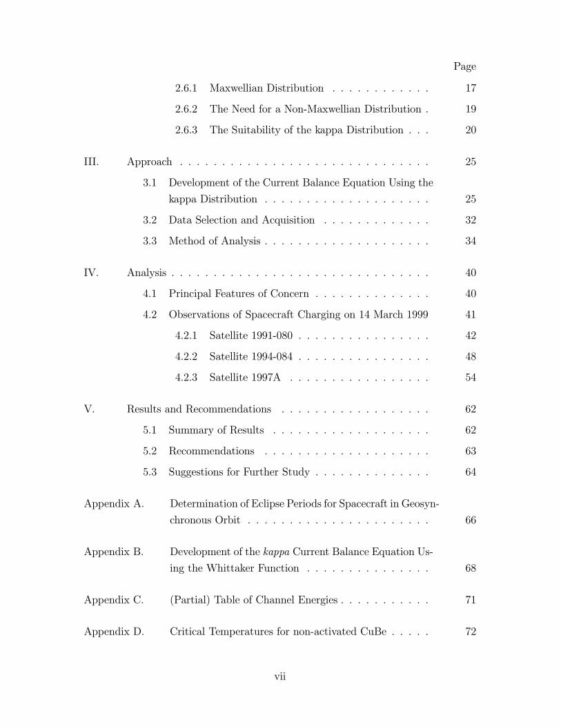
List of FiguresFigure Page

1. Secondary (δe - dot), backscattered (ηe - dash), and δe + ηe

(solid) electron emission coefficients due to normal incidence of

primary electrons on a surface composed of non-activated CuBe

vs. primary electron energy ε. . . . . . . . . . . . . . . . . . 7

2. Correlation Between Spacecraft Potential and Electron Temper-

ature from LANL 1994-084 Measurements Taken on 14 March

1999. The line at −2 kV highlights the period of spacecraft

eclipse. (Data courtesy of Michelle F. Thomsen, Los Alamos

National Laboratory.) . . . . . . . . . . . . . . . . . . . . . . 11

3. Spacecraft Charging in Sunlight vs. Charging in Eclipse as

Determined from LANL 1994-084 Measurements Taken on 14

March 1999. (Data courtesy of Michelle F. Thomsen, Los Alamos


4. kappa velocity distributions (Equation (??)) for κ = 3 (solid

line) and κ = 6 (dashed line), respectively, plotted versus the

speed normalized to the most probable speed. The limiting case

κ→∞, which is simply the Maxwell distribution exp(−v2/w2),and which has the same most probable speed is superimposed. 21

5. Electron Distribution Function vs. Electron Energy for LANL

1991-080 Data at 22.04 UT (22.57 LT) on 14 March 1999 Demon-

strating Superiority of the kappa Distribution over the Maxwellian

at Capturing the High Energy Tail. Plotted are LANL Data

Values (circles), kappa Distribution (solid), and Maxwellian Dis-

tribution (dash). (Data Courtesy of Michelle F. Thomsen, Los

Alamos National Laboratory.) . . . . . . . . . . . . . . . . . 23

6. Normalized Current I/I0 vs. Electron Temperature for non-

activated CuBe. Curves are the kappa Current Balance Equa-

tion with κ = 1.6 (dot), κ = 2.5 (dash-dot), κ = 5.5 (dash),

and the Maxwellian Current Balance Equation (solid). . . . . 30

ix

Figure Page

7. Normalized Current I/I0 vs. Electron Temperature for kapton.

Curves are the kappa Current Balance Equation with κ = 1.6

(dot), κ = 2.5 (dash-dot), κ = 5.5 (dash), and the Maxwellian

Current Balance Equation (solid). . . . . . . . . . . . . . . . 32

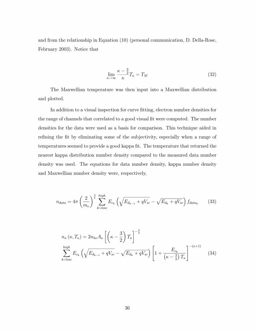
8. Electron Distribution Function vs. Electron Energy for LANL

1994-084 Data taken at 16.67 UT (23.57 LT) on 09 March

1999. Plotted are LANL data values (circles), kappa distri-

bution (solid line), and Maxwellian Distribution (dash). (Data

Courtesy of Michelle F. Thomsen, Los Alamos National Labo-

ratory.) . . . . . . . . . . . . . . . . . . . . . . . . . . . . . 38

9. Electron Distribution Function vs. Electron Energies for LANL

1994-084 Data taken at 16.79 UT (23.69 LT) on 09 March

1999. Plotted are LANL data values (circles), kappa distri-

bution (solid line), and Maxwellian Distribution (dash). (Data

Courtesy of Michelle F. Thomsen, Los Alamos National Labo-

ratory.) . . . . . . . . . . . . . . . . . . . . . . . . . . . . . 39

10. Spacecraft Potential and Electron Temperature Curves for LANL

1991-080 on 14 March 1999/16-24 UT. The black line at −2kV potential shows the period of eclipse. (Data Courtesy of

Michelle F. Thomsen, Los Alamos National Laboratory.) . . . 42

11. Electron Distribution Function vs. Electron Energy at 20.90

UT (21.42 LT) on 14 March 1999 from LANL 1991-080 Data.

Displayed are the Data Derived (circles), the kappa (solid), and

the Maxwellian (dash) Distribution Functions. (Data Courtesy

of Michelle F. Thomsen, LANL.) . . . . . . . . . . . . . . . . 43

12. Electron Distribution Function vs. Electron Energy at 20.90 UT

(21.42 LT) on 14 March 1999 from LANL 1991-080 Data. The

Fit is with Respect to the Maxwellian Temperature. Displayed

are the Data Derived (circles) and the Maxwellian (dash) Dis-

tribution Functions. (Data Courtesy of Michelle F. Thomsen,

LANL.) . . . . . . . . . . . . . . . . . . . . . . . . . . . . . . 44

x

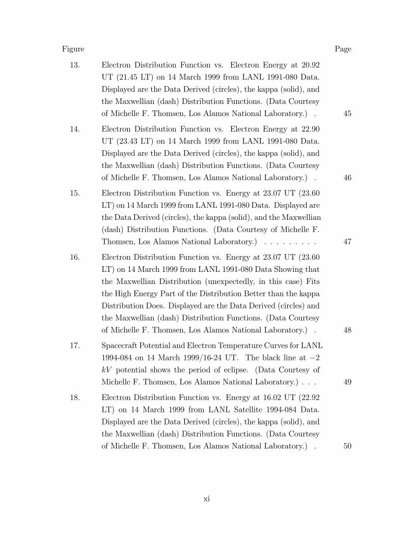
Figure Page





of Michelle F. Thomsen, Los Alamos National Laboratory.) . 45






15. Electron Distribution Function vs. Energy at 23.07 UT (23.60

LT) on 14 March 1999 from LANL 1991-080 Data. Displayed are

the Data Derived (circles), the kappa (solid), and the Maxwellian

(dash) Distribution Functions. (Data Courtesy of Michelle F.

Thomsen, Los Alamos National Laboratory.) . . . . . . . . . 47


LT) on 14 March 1999 from LANL 1991-080 Data Showing that

the Maxwellian Distribution (unexpectedly, in this case) Fits

the High Energy Part of the Distribution Better than the kappa

Distribution Does. Displayed are the Data Derived (circles) and




1994-084 on 14 March 1999/16-24 UT. The black line at −2kV potential shows the period of eclipse. (Data Courtesy of



LT) on 14 March 1999 from LANL Satellite 1994-084 Data.




xi

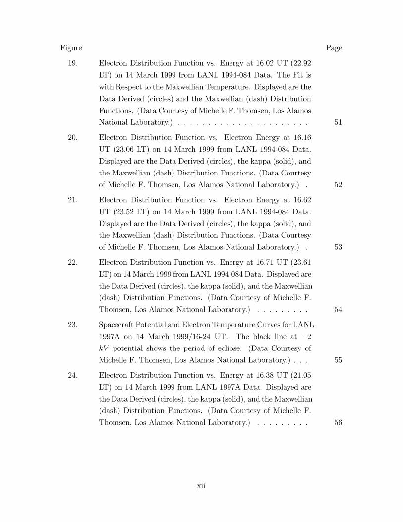
Figure Page


LT) on 14 March 1999 from LANL 1994-084 Data. The Fit is

with Respect to the Maxwellian Temperature. Displayed are the

Data Derived (circles) and the Maxwellian (dash) Distribution

Functions. (Data Courtesy of Michelle F. Thomsen, Los Alamos


















1997A on 14 March 1999/16-24 UT. The black line at −2kV potential shows the period of eclipse. (Data Courtesy of



LT) on 14 March 1999 from LANL 1997A Data. Displayed are




xii

Figure Page


LT) on 14 March 1999 from LANL 1997A Data. The Fit is

with Respect to the Maxwellian Temperature. Displayed are the

Data Derived (circles) and the Maxwellian (dash) Distribution

Functions. (Data Courtesy of Michelle F. Thomsen, Los Alamos



UT (21.17 LT) on 14 March 1999 from LANL 1997A Data.





UT (21.17 LT) on 14 March 1999 from LANL 1997A Data. The

Fit is with Respect to the Maxwellian Temperature, and the

Potential is−45 V . Displayed are the Data Derived (circles) andthe Maxwellian (dash) Distribution Functions. (Data Courtesy



UT (21.65 LT) on 14 March 1999 from LANL 1997A Data.





LT) on 14 March 1999 from LANL 1997A Data. Displayed are




xiii

List of TablesTable Page

1. (Partial) Table of Channel Energies . . . . . . . . . . . . . . 71

2. Critical Temperatures for CuBe (non-activated) with kappa =

2.5 to 17.5 . . . . . . . . . . . . . . . . . . . . . . . . . . . . 72

xiv

AFIT/GAP/ENP/03-05

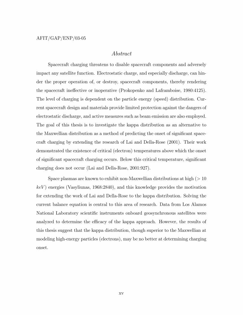
Abstract

Spacecraft charging threatens to disable spacecraft components and adversely

impact any satellite function. Electrostatic charge, and especially discharge, can hin-

der the proper operation of, or destroy, spacecraft components, thereby rendering

the spacecraft ineffective or inoperative (Prokopenko and Laframboise, 1980:4125).

The level of charging is dependent on the particle energy (speed) distribution. Cur-

rent spacecraft design and materials provide limited protection against the dangers of

electrostatic discharge, and active measures such as beam emission are also employed.

The goal of this thesis is to investigate the kappa distribution as an alternative to

the Maxwellian distribution as a method of predicting the onset of significant space-

craft charging by extending the research of Lai and Della-Rose (2001). Their work

demonstrated the existence of critical (electron) temperatures above which the onset

of significant spacecraft charging occurs. Below this critical temperature, significant

charging does not occur (Lai and Della-Rose, 2001:927).

Space plasmas are known to exhibit non-Maxwellian distributions at high (> 10

keV ) energies (Vasyliunas, 1968:2840), and this knowledge provides the motivation

for extending the work of Lai and Della-Rose to the kappa distribution. Solving the

current balance equation is central to this area of research. Data from Los Alamos

National Laboratory scientific instruments onboard geosynchronous satellites were

analyzed to determine the efficacy of the kappa approach. However, the results of

this thesis suggest that the kappa distribution, though superior to the Maxwellian at

modeling high-energy particles (electrons), may be no better at determining charging

onset.

xv

SPACECRAFT CHARGING




I. Introduction

1.1 Objective

The goal of this research is to refine the correlation of spacecraft charging at

geosynchronous altitudes to a threshold temperature above which significant space-

craft charging can occur. Emphasis is placed on the accumulation of charge on the

spacecraft surface (surface charging). In an effort to reach the stated goal, an ana-

lytical formulation of the current-balance equation using a kappa distribution will be

accomplished. A numerical comparison of the theoretical results against observations

will be used to evaluate the success of the approach.

1.2 Motivation

Spacecraft charging threatens to disable spacecraft components and adversely

impact any satellite function. Electrostatic charge, and especially discharge, can

destroy the functionality of components or components themselves, thereby ren-

dering them ineffective or inoperative (Prokopenko and Laframboise, 1980:4125).

Additionally, a local environment consisting of excess charge can interfere with data

collection, causing measurements taken by spacecraft instruments to be misleading

and giving rise to improper conclusions about the space environment (DeForest,

1972:659; Lai, 1999:3). Presently, spacecraft design and materials provide limited

protection against the dangers of electrostatic discharge.

1

Environmental assessment and space weather event forecasting, including fore-

casts of operational impacts of space weather, are among the primary missions of Air

Force Weather Agency space weather operations. Informing space systems operators

of when and where spacecraft charging can occur with sufficient warning time can

aid in minimizing adverse operational impacts such as permanent damage to space

assets. Furthermore, post-event engineering assessments of satellite failures can be

improved if we can tell the satellite operators that charging did (or did not) play a

role in a given failure.

The current balance equation reveals the limiting conditions for which the

current into a surface element equals the current out of the element. Outside of these

conditions, the net current is nonzero — i.e., charging can occur. Thus, the solution

of the current balance equation is central to solving charging-related problems.

1.3 Scope

This study aims to refine the process of determining the critical temperature

for the onset of spacecraft charging by incorporating the kappa distribution solution

of the current balance equation as noted above. This research will examine data

from Los Alamos National Laboratory (LANL) instruments aboard United States

Department of Energy satellites 1997A, 1994-084, and 1991-081 from the following

time frames: March and April 1999; March, June, and September 2000. The time

periods were selected to coincide with previous work by Lai and Della-Rose (2001)

as an extension for a non-Maxwellian plasma environment.

Eclipse events and a coronal mass ejection (CME) event will be examined.

These two types of events fit the common theme of previous research and so will be

useful for comparison of results. When the plane of the satellite’s orbit intersects

the earth-sun line, the satellite will be eclipsed by the earth’s shadow near local mid-

night. Spacecraft charging can result from various mechanisms. The mechanisms

we will explore are charging due to ambient plasma (ions and electrons), secondary

2

and backscattered electrons, and photoelectrons as well as charging associated with

combinations of these particles. In this analysis, only charging due to ambient ions

and electrons combined with secondary and backscattered electrons will be modeled

mathematically. Other types of charging include differential charging, beam charg-

ing, bootstrap charging, and mechanically induced charging. These latter types are

outside the scope of this thesis.

3

II. Background

This chapter will describe key parameters associated with spacecraft charging

at geosynchronous orbit (GEO). First, the plasmasphere, which GEO spacecraft

encounter daily will be covered. This will be followed by a brief description of

particles responsible for spacecraft charging along with their associated distributions

and energies outside the plasmasphere, where significant spacecraft charging tends to

occur. Then a brief introduction to spacecraft charging will be presented. Finally,

various charging scenarios will be discussed. The convention adopted here will be

to represent particle temperatures in terms of energy (eV ) — i.e., T = kBT ., where

kB = 1.3806568× 10−23 JK−1 = 8.617385× 10−5 eVK−1 is Boltzmann’s constant.

2.1 Spacecraft Environment at Geosynchronous Altitudes

The following sections will describe environmental factors affecting spacecraft

at GEO. First, we will examine the plasmasphere, which is not normally associated

with significant charging. This will be followed by a description of particles that in-

fluence spacecraft charging, including number densities and distributions associated

with each type of particle.

2.1.1 Plasmasphere. The plasmasphere is a near-Earth region containing

cold (∼ 1 eV ), dense plasma. Electron densities in the plasmasphere typically range

from 10 to 104 cm−3 (Su, et al., 2001:1185). It extends from the terrestrial ionosphere

into space over ranges of about 1 to 7 RE, where 1 RE is the radius of the Earth (6370

km). If the spacecraft is within the plasmasphere, the relatively dense (> 1.0 cm−3)

and cool (∼ few eV ) plasma can envelop the satellite. Charging in this region is

often induced by the photoelectric effect, which typically results in potentials of only

a few volts (DeForest, 1972:655, 659). This charging process is further explained in

Section 2.2.2.2. At the plasmapause, first noted independently by Carpenter (1963)

and Gringauz (1963), electron densities tend to drop considerably. The location of

4

the plasmapause varies with the level of geomagnetic activity (Carpenter, 1963), and

it can extend beyond geosynchronous altitudes during “quiet times” (Kp < 2). Kp

is a logarithmic, planetary index (0 to 9) of the disturbance of the geomagnetic field,

with higher values implying greater disturbances (Parks, 1991:512).

2.1.2 Plasma Densities at Geosynchronous Altitudes. Beyond the plasma-

pause, electron densities are typically about 0.1 to 3 cm−3 at geosynchronous alti-

tudes depending on the local time of the spacecraft and the level of geomagnetic

activity.

2.1.3 Gradient-Curvature Drift. At geosynchronous altitudes, a gradient-

curvature drift induced by the Earth’s magnetic field determines the directions of

the electrons and positively charged ions (see, for example, Kivelson and Russell,

1995:310-312). This gradient-curvature drift causes electrons to flow eastward and

ions to flow westward. Thus, even after local midnight, a GEO spacecraft may

experience significant charging due to electron currents.

2.1.4 Key Particle Descriptions and Distributions. The following sections

describe electrons from various sources as well as (positive) ions and their associated

distributions and fluxes at GEO. These particles, and their distributions with respect

to kinetic energy, dictate the charging environment of GEO satellites.

2.1.4.1 Ambient Ions and Electrons. Ambient ion and electron den-

sities are approximately 0.1 to 1.0 cm−3 at GEO. With the injection of magnetotail

plasma, the density can increase to approximately 3.0 cm−3 (Hastings and Garrett,

1996:69-70).

2.1.4.2 Photoelectrons. Photoelectrons are created when photons

strike the spacecraft surface and impart enough energy to induce electron emission

from the spacecraft surface. Typical photoelectron energy is only a few eV (Hastings

5

and Garrett, 1996:148; Lai, 1999:5). Since photon densities are very high, photoelec-

tron densities will be proportionately large. The number of photoelectrons produced

and their energies are largely dependent on spacecraft material properties and design

(Hastings and Garrett, 1996:147-148). The number flux of photoelectrons tends to

be much greater than that of ambient electrons.

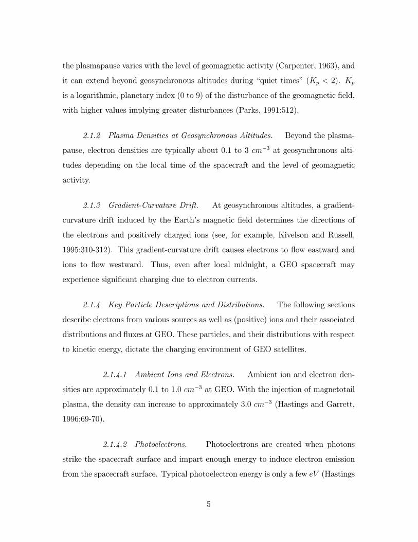
2.1.4.3 Secondary and Backscattered Electrons. When electrons

strike a spacecraft, they will either be reflected or absorbed. If they are of low

enough energy, they will be reflected. The reflection coefficient is approximately

0.05 (Hastings and Garrett, 1996:148) — that is, most electrons are absorbed. When

electrons are absorbed, they will either collide with other electrons and backscatter or

produce secondary electrons (explained below). Backscattered electrons are primary

electrons that are ejected after they penetrate the surface. These electrons typically

have slightly lower energy than they had upon impact. Sternglass (1954:345,352-

356) considered backscattered electrons as those emitted with energies greater than

50 eV , and he found their energies to be about 12of that of incident electrons for

primary energies of 0.2 to 32 keV . For this discussion, backscattered electrons can

be incorporated as a reduction factor for incident electrons (Hastings and Garrett,

1996:149,169-170). The probability that backscattered electrons are emitted is de-

noted by η(ε). Sternglass considered emitted electrons with energies below 50 eV as

secondary electrons, and this is the convention adopted here.

Secondary electrons are emitted when a primary, high-energy, electron pene-

trates the spacecraft surface and imparts enough energy to neighboring electrons that

these neighboring electrons can escape. If the energy of the primary electrons is large

enough, but not too large, secondary electrons may be ejected. Also, energy from

the primary electron may be imparted to more than one neighboring electron. So

it is possible, even probable over some energy ranges, that the number of secondary

electrons leaving the spacecraft surface is greater than the number of incoming — i.e.,

δ(ε) > 1, where δ(ε) is the probability of secondary electron emission.

6

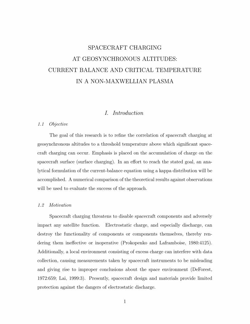
Figure 1 illustrates the dependence of secondary and backscattered electron

emission on the primary energy of electrons impacting the spacecraft surface com-

posed of non-activated CuBe with normal incidence. Secondary and backscattered

yield curves are based on data fits derived by Sanders and Inouye (1978) and

Prokopenko and Laframboise (1980), respectively. Note that in this example, δ(ε) =

1 for primary electron energies of about 0.05 and 1.42 keV . Observe that δ(ε) < η(ε)

up to about 10 eV , and that the sum δ(ε)+η(ε) approaches a constant (0.31) as the

primary energy approaches 10 keV .

1 .10 3 0.01 0.1 1 10 1000

0.5

1

1.5

2

2.5

Primary Electron Energy (keV)

Seco

ndar

y/B

acks

catte

red

Elec

tron

Yie

ld

I II III

Figure 1 Secondary (δe - dot), backscattered (ηe - dash), and δe+ηe (solid) electron

emission coefficients due to normal incidence of primary electrons on a

surface composed of non-activated CuBe vs. primary electron energy ε.

7

2.2 Spacecraft Charging

Garrett (1981:577-579) gives an historical overview of spacecraft charging and

related research up to 1981. He characterizes associated research into four distinct

periods, beginning with the use of the Langmuir probe. He notes, “The first example

of a spacecraft charging effect is in a paper by Johnson and Meadows [1955].” Large

negative potentials (−20 kV ) were observed in eclipse on Applications TechnologySatellite 6 (ATS-6) (1981:578) in the 1970’s. Such potentials are characteristic of

particle distributions that are well represented by the kappa distribution. DeForest

(1972) was the first to note spacecraft charging at GEO.

Spacecraft charging is the buildup of potential on a spacecraft relative to that

of the ambient (surrounding the spacecraft) plasma. By convention, the potential

of the ambient space plasma is taken to be zero. When the spacecraft potential is

nonzero relative to the space plasma, the spacecraft is charged. Spacecraft charging

includes, but is not limited to, surface charging, frame charging, differential charging

and deep dielectric charging. It is induced by a local difference in ion and electron

fluxes (Lai, 1999:4), and most GEO spacecraft often charge to about 0.2 — 1 keV .

(Hastings and Garrett, 1995:149; Lai, 1999:5).

Negative charging is predominant since the electron flux is about two orders of

magnitude greater than the ion flux. This is a natural consequence of the differences

in magnitude of the particle masses — i.e., if the electron and ion energies are assumed

to be approximately equal, then the ratio of the electron velocity to the ion velocity

is approximately equal to the inverse square root of the ratio of the ion mass to the

electron mass. Therefore, in a quasi-neutral gas, the particle flux ratio varies as the

ratio of the particle velocities.

2.2.1 The Thick Sheath Limit. When examining spacecraft charging at

GEO vs. low- or middle- Earth orbit, it is important to note the distinction between

thin and thick sheath limits. Hastings and Garrett define the sheath as the region

8

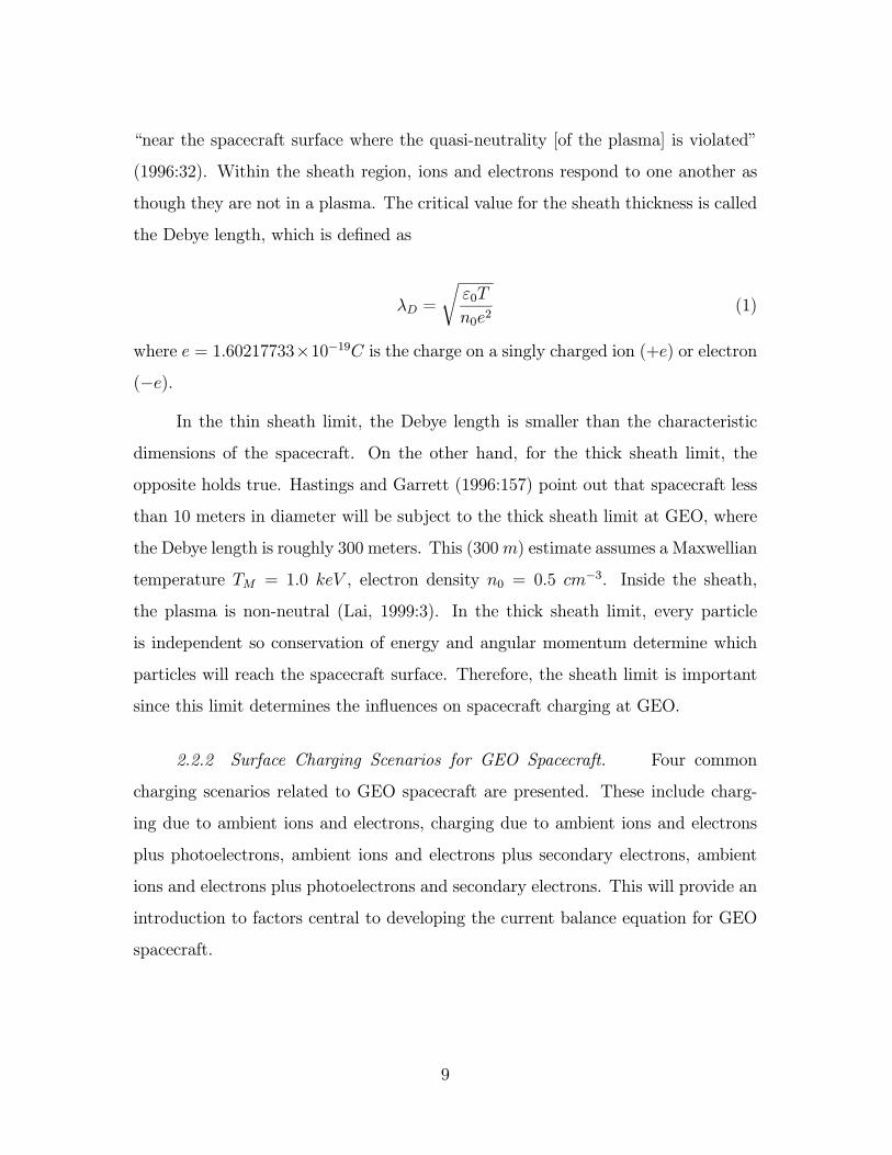
“near the spacecraft surface where the quasi-neutrality [of the plasma] is violated”

(1996:32). Within the sheath region, ions and electrons respond to one another as

though they are not in a plasma. The critical value for the sheath thickness is called

the Debye length, which is defined as

λD =

rε0T

n0e2(1)

where e = 1.60217733×10−19C is the charge on a singly charged ion (+e) or electron(−e).

In the thin sheath limit, the Debye length is smaller than the characteristic

dimensions of the spacecraft. On the other hand, for the thick sheath limit, the

opposite holds true. Hastings and Garrett (1996:157) point out that spacecraft less

than 10 meters in diameter will be subject to the thick sheath limit at GEO, where

the Debye length is roughly 300 meters. This (300m) estimate assumes a Maxwellian

temperature TM = 1.0 keV , electron density n0 = 0.5 cm−3. Inside the sheath,

the plasma is non-neutral (Lai, 1999:3). In the thick sheath limit, every particle

is independent so conservation of energy and angular momentum determine which

particles will reach the spacecraft surface. Therefore, the sheath limit is important

since this limit determines the influences on spacecraft charging at GEO.

2.2.2 Surface Charging Scenarios for GEO Spacecraft. Four common

charging scenarios related to GEO spacecraft are presented. These include charg-

ing due to ambient ions and electrons, charging due to ambient ions and electrons

plus photoelectrons, ambient ions and electrons plus secondary electrons, ambient

ions and electrons plus photoelectrons and secondary electrons. This will provide an

introduction to factors central to developing the current balance equation for GEO

spacecraft.

9

2.2.2.1 Ambient Ions and Electrons. First we will examine the am-

bient ion and electron charging environment while neglecting photoelectrons and

secondary and backscattered electrons. To begin, we determine whether the space-

craft will charge positively or negatively, if at all. Consider the flux, Γ = nu, of ions

and electrons at zero spacecraft potential, where u is the particle (electron or ion)

velocity, and suppose that ne = ni as for a quasi-neutral plasma. Since me << mi,

if we assume that the ion and electron energies are approximately the same, then

ue >> ui, so the electron flux is much greater than the ion flux, and the electron

current causes the spacecraft to accumulate a negative charge, which will eventually

serve as a potential barrier to incoming electrons, as well as enlarge the ion current.

Now to determine how much the spacecraft charges, we seek an equilibrium

state where the net flux–and therefore the net current–is zero. Without loss of

generality, consider that the spacecraft charges to some negative potential, Vsc, re-

sulting in a potential barrier with energy, eVsc. Incoming electrons with kinetic

energy, T < eVsc, will not be able to penetrate the barrier. So the number flux of

electrons is limited, and an equilibrium state is achieved once the number flux of

ions and electrons is equal. Note that the thermal energy of the electrons (electron

temperature) is pivotal to determining how much charge will accumulate (Hastings

and Garrett, 1996:168).

2.2.2.2 Ambient Ions and Electrons and Photoelectrons. Now con-

sider the case of the spacecraft in sunlight (without regard for secondary and backscat-

tered electrons). This can result in large numbers of photoelectrons being emitted

from the spacecraft.

Recall that the number density of photoelectrons is much greater than that

of ambient electrons. This results in a net positive charge about the sunlit surface.

Since photoelectrons are directed away from the spacecraft, the resulting net posi-

tive potential will serve to attract escaping photoelectrons. However, photoelectron

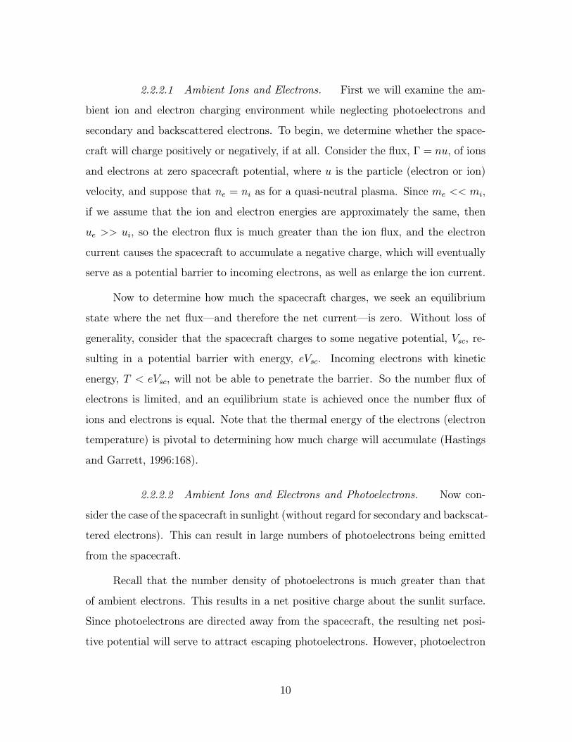
10

energy is typically only a few eV , so the total charge about a sunlit surface typically

can reach only a few volts positive.

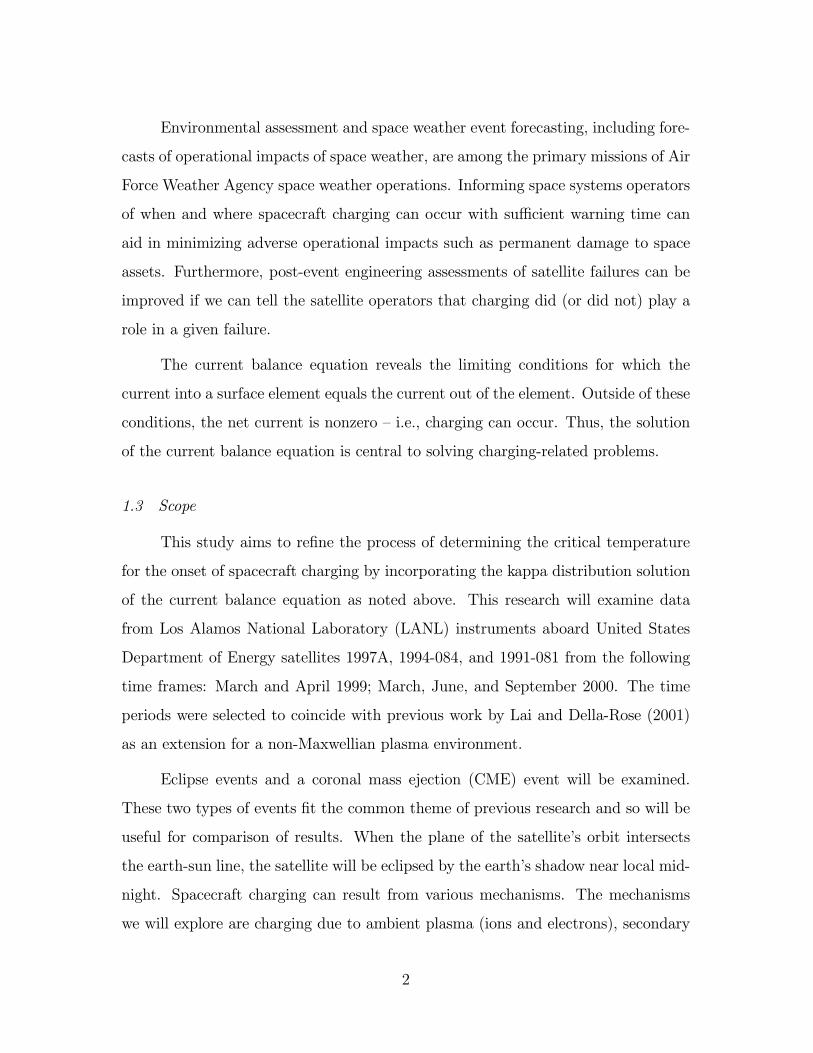
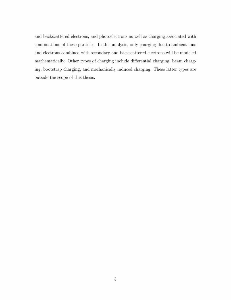
Figures 2 and 3 illustrate the dependence of potential on temperature and are

prime examples of the distinct differences between charging in sunlight vs. charging

in eclipse. Notice that when the spacecraft is in eclipse it can reach much larger

potentials than when it charges in sunlight. Measurements are from LANL 1994-084

data on 14 Mar 1999, and spacecraft local time is approximately six hours later than

UT. The period of eclipse is highlighted in Figure 2 by the line at −2 kV . Alsoevident in Figure 3 is a threshold temperature for significant charging to begin. The

determination of eclipse periods is described in Appendix A.

0 4 8 12 16 20 244

2

0

2

4

6

Time (UT)

Pote

ntia

l (kV

)

T

empe

ratu

re (k

eV)

Figure 2 Correlation Between Spacecraft Potential and Electron Temperature

from LANL 1994-084 Measurements Taken on 14 March 1999. The line

at −2 kV highlights the period of spacecraft eclipse. (Data courtesy of

Michelle F. Thomsen, Los Alamos National Laboratory.)

11

0 0.5 1 1.5 2 2.5 3 3.5 4 4.50

0.5

1

1.5

2

2.5

3

Temperature (keV)

Pote

ntia

l (kV

)

Spacecraft in Eclipse

Spacecraft in Sunlight

Figure 3 Spacecraft Charging in Sunlight vs. Charging in Eclipse as Determinedfrom LANL 1994-084 Measurements Taken on 14 March 1999. (Datacourtesy of Michelle F. Thomsen, Los Alamos National Laboratory.)

2.2.2.3 Ambient ions and electrons and secondary electrons. As an

introduction, this discussion will cover a monoenergetic energy distribution of the

ambient electrons and ions. The case of an energy distribution over a range of

energies is presented in Section 2.6. Recall that backscattered electrons serve as

a scaling factor for the incident electron flux, and so they are absorbed into the

ambient electron flux term.

Now consider the three regions I, II, and III of in Figure 1 (ignoring the contri-

bution of photoelectrons), where the regions are delimited according to the secondary

electron yield (dotted line). In region I, the primary energy is too low to force emis-

sion of more electrons than are incident on the surface. That is, the incoming flux

will be greater than the outgoing flux, but with low kinetic energy less than that

of the first crossing where δ(ε) = 1, and the electron current causes the spacecraft

12

to accumulate a negative charge dependent on the ambient plasma electron temper-

ature (Rubin, et al., 1980:9). For a monoenergetic beam, the maximum potential

attained will be no greater than the voltage equivalent corresponding to the δ(ε) = 1

energy at the region I boundary.

In region II, the energy of the primary electrons is in the range where the

number of secondary electrons produced exceeds the number of incident electrons,

so the incoming flux of electrons will be less than the outgoing flux. Therefore, the

secondary electrons will determine the amount of spacecraft charging, which will

be positive with a potential corresponding to the energy of the outgoing secondary

electrons. Since secondary electrons are of relatively low energy, the overall potential

is typically not substantial.

In region III, the primary energy is so great that incident electrons may pen-

etrate too quickly for neighboring electrons at the surface to respond. That is, the

primaries may not spend enough time next to prospective secondary electrons to

impart sufficient energy for them to escape. Additionally, incident electrons can

penetrate so deeply that secondary electrons will not have enough energy to es-

cape. Thus the secondary yield decreases to a value less than unity at these higher

energies, and the ambient electron temperature again determines the spacecraft po-

tential. Consistent with the high electron temperature in this region, we can expect

spacecraft charging to large potentials (> 1 kV ). When a spacecraft is in eclipse

(i.e., no photoelectrons present), the charging will be determined by the ambient ion

and electron and secondary electron considerations noted here.

The energy corresponding to the δ(ε) = 1 transition between regions II and

III has an electron temperature associated with it. Based on the preceding dis-

cussion, above this electron temperature, the primary electron flux is greater than

the secondary electron flux, and significant negative charging can occur. For a mo-

noenergetic incident electron flow, this temperature at which δ(ε) = 1 is the critical

temperature.

13

2.2.2.4 Ambient Ions and Electrons, Photoelectrons, and Secondary Elec-

trons. Finally, we consider the combined influence of ambient ions and electrons,

photoelectrons, and secondary and backscattered electrons. This will be the case

when the spacecraft is in sunlight. On the sunlit side of the spacecraft, the photo-

electron emission will dominate. While on the dark side, if δ(ε) < 1, ambient ion

and electron flux will determine charging, but if δ(ε) ≥ 1, the secondary electronemission will rule. In both cases, differential charging tends to occur even if the

sunlit side swings negative since the dark side will tend to charge more negatively

than the sunlit side. Once the sunlit side is charged to a few volts, a positively

charged barrier potential begins to form. This barrier potential (a “saddle point”

in the potential sunward of the spacecraft that causes a sunward-directed electric

field between the satellite and the “minimum” of the saddle) grows as differential

charging develops across the spacecraft (since one side is sunlit and the other is in

darkness). Eventually, the barrier potential prevents photoelectrons from escaping

the satellite, and large negative potentials can result. (Hastings & Garrett, 1996:176;

private communication, D. Della-Rose, January 2003).

Recall that the charging discussion above is associated with monoenergetic

ambient electrons, and this constraint will be relaxed in Section 2.6.

2.3 Charging Associated with Eclipse and Coronal Mass Ejections

DeForest (1972:655) states that a GEO spacecraft goes into eclipse for about

12hour every night for a period of about 3 to 4 weeks on either side of equinox.

For the data examined in the present research, the duration of eclipse approached

one hour by 16 March 1999. An example of this is illustrated in Figure 2 above.

DeForest (1972:651) determined that ATS-5 could charge to potentials as high as 10

kV during eclipse and 200 V in sunlight.

CMEs also provide relatively large amounts of solar plasma, which is injected

into the geosynchronous orbit of the spacecraft. During both eclipse charging events

14

and CMEs, the plasma is typically high-energy, but not necessarily dense. However,

Hastings and Garrett (1996:69-70) indicate that the plasma density and high-energy

portion of the distribution function increase during geomagnetic storming. This

concept is consistent with the injection of magnetotail plasma into the near-Earth

environment, in addition to the plasma already present. They conclude that this

increase in the high-energy distribution has a decisive impact on spacecraft charging.

This, too, is consistent with the higher potentials reached as the plasma density and

high-energy portion of the distribution function increased as evidenced in the data

examined.

The level of charging is also related to the Kp value (Garrett, 1981:580,584).

Higher Kp values imply greater disturbances, which follows from higher energy

plasma impinging on the near-Earth region (Kivelson and Russell, 1995:294-295).

These higher particle energies can result in large spacecraft surface potentials.

2.4 Measurement of Spacecraft Potentials

A charged spacecraft attracts charged particles of the opposite sign and repels

those of the same sign, resulting in an energy shift where the energies of ions and elec-

trons inside the sheath are different from those outside the sheath. Since we consider

the ambient plasma (outside the sheath) to be at zero potential, this shift represents

the spacecraft potential. When hot plasma is injected into geosynchronous orbit, the

hot electron flux increases, causing a satellite to charge to large negative potentials

with respect to the ambient environment. This negative potential accelerates the

low-energy (v 0 eV ) ions arriving at the spacecraft, shifting ion energies by qVsc.

The charged spacecraft, on the other hand, repels the electrons, and this repulsion

results in the electrons with energies between 0 and qVsc not being measured since

they don’t reach the spacecraft surface (Lai, 1999:4).

If the low-energy ambient ion density is large enough, acceleration through the

spacecraft sheath produces a distinct gap, or narrow peak, in the ion energy distri-

15

bution (i.e., an ion line) at the spacecraft potential, which can be easily identified

on spectrograms or by instruments, providing a clearly identifiable measure of the

potential. If no ion line is found, the spacecraft potential can be determined through

iterative procedures (Garrett, 1981:580-581; Lai, 1999:3-4; Thomsen, et al., 1999:11-

13). Though measurement of potentials is outside the scope of this research, the

measured potentials are central to calculating corrected energies (cf. Section 3.3).

2.5 The Current Balance Equation

As previously noted, charging occurs due to an imbalance of incoming versus

outgoing flux of charged particles, namely, electrons and (positive) ions. The prin-

cipal particle fluxes for charging onset are those of incident electrons and secondary

electrons. Strictly speaking, this is true only in eclipse, where photoelectrons are

not a factor. Considering the argument in Section 2.2.2.4, we note that the barrier

potential has an effect on the current balance outside of eclipse as well. Thus, differ-

ential charging effects can cause large negative charging events to commence outside

of eclipse. Again, our study does not attempt to model such effects.

With regard to electron flux, the incoming electron flux is balanced by the out-

going secondary emission and backscattered electrons at the critical temperature. As

noted above, we can neglect the ion flux (for charging onset) since it is approximately

two orders of magnitude smaller than the electron flux.

Now consider a distribution of ambient electron energies in regions II and III

(as opposed to the earlier monoenergetic assumption). While the portion of the

distribution with energies corresponding to region II will result in a net flux of

outgoing electrons, the part of the ambient distribution with energies in the range

of region III will result in a net flux of electrons toward the spacecraft. When these

two fluxes balance, the net current to the spacecraft is zero. The temperature T ,

where this balance occurs, is the critical temperature. But when the net electron

flux toward the spacecraft (region III) exceeds the net outgoing flux (region II), the

16

spacecraft will charge negatively. More importantly, the spacecraft can charge to

high negative voltages. Equation (6) gives a mathematical definition of the critical

temperature.

The mathematical implementation of the Maxwellian distribution is explained

in Section 2.6.1, and the implementation of the kappa distribution is in Section 3.1.

2.6 Critical Temperature

Rubin, et al., observed a threshold electron temperature below which ATS-5

instruments did not detect charging and above which charging occurred. In the

spacecraft charging arena, this threshold temperature is commonly referred to the

“critical temperature” for the onset of spacecraft charging. The associated spacecraft

potential varied almost linearly with the electron temperature above this threshold

(Rubin, et al., 1980:6, 9). Lai (1991) provides a theoretical basis for calculating

the critical temperature. This threshold temperature commonly appears in the 1.5

- 2.5 keV range (Lai and Tautz, 2001:11), and this range is consistent for various

spacecraft surface materials and configurations.

Up to now, research related to the calculation of the critical temperature has

been limited to the Maxwellian approach.

2.6.1 Maxwellian Distribution. It is appropriate to convert the velocity

moment into terms of energy to obtain

Z ∞

0

v3F (v)dv =

Z ∞

0

εf(ε)dε (2)

where the distribution functions are appropriately normalized. Here, F (v) is the

velocity distribution. In the Maxwellian model, the energy distribution f (ε), for a

given mass m, density n, and Maxwellian temperature TM , is

17

fM(ε) = n

µm

2πTM

¶32

e(− ε

TM)ε12 (3)

The secondary electron, δ(ε), and backscatter, η(ε), coefficients are measured

as functions of energy, where

δ(ε) = c(e−εa − e− ε

b ) (4)

and

η(ε) = A−Be−εC (5)

as determined (by data fits) by Sanders and Inouye (1978:74) and Prokopenko and

Laframboise (1980:4127), respectively. Here a = 4.3Emax, b = 0.367Emax and

c = 1.37δmax. δmax is the maximum value of δ(ε), and Emax is the primary elec-

tron energy corresponding to δmax (Lai, 1991:1630). Prokopenko and Laframboise

(1980:4127) state, “The coefficients A,B, and C are functions of the atomic number

Z of the surface material.” To emphasize, these values are material dependent. It is

convenient to calculate the current balance in terms of energy (cf. Lai, 1991:1630).

When the incident electron flux is balanced by the secondary and backscattered flux,

the spacecraft potential is zero, and we can write the current balance equation as

Z ∞

0

ε12f(ε)dε =

Z ∞

0

ε12f(ε)[δ(ε) + η(ε)]dε (6)Z ∞

0

εe(− ε

TM)dε =

Z ∞

0

εe(− ε

TM)[c(e−

εa − e− ε

b ) +A−Be−εC ]dε (7)

where Equation (6) is valid for an arbitrary energy distribution function, and Equa-

tion (7) follows when the distribution function in Equation (3) is substituted into

Equation (6). Observe that the normalization constants divide out since fM (ε) is

18

a term on both sides of the equation, so there is no dependence on electron density

(Lai, 1991:1630). Recall that ion flux is omitted since it is not substantial when con-

sidering spacecraft charging onset. Integrating Equation (6) and simplifying yields

c[(1 +TMa)−2 + (1 +

TMb)−2] +A−B(1 + TMC)−2 − 1 = 0 (8)

The solution TM of this equation is the critical temperature for charging onset,

assuming a Maxwellian plasma. Strictly speaking, this equation is valid for spacecraft

in eclipse since photoelectrons are not considered. Note that the resulting critical

temperature is material dependent. For example, the critical temperature is 1.341

keV for non-activated CuBe, and 0.5 keV for kapton. Both of these materials are

examined in the present research. Lai and Della-Rose (2001:923) present a table of

critical temperatures (rounded up to the next 0.1 keV ) for various materials.

2.6.2 The Need for a Non-Maxwellian Distribution. For relatively low-

energy particles (∼ 10 keV or less) in space, the Maxwell distribution gives accurate

results for electron and ion velocity distributions (Meyer-Vernet, 2001:248). We

expect the Maxwell distribution to be representative since lower thermal energies

(particle velocities) result in larger collision cross-sections. Conversely, as velocities

increase, cross-sections decrease. Thus it follows that the collisional properties of a

gas would become less dominant.

Therefore, the weakness of the Maxwell distribution for space plasmas at or

near geosynchronous satellite orbits is attributable to the fact that the thermal en-

ergy (velocity) is high while the density is often low. Thus the mean free path of

particles sometimes becomes greater than the scale height, which is the length-scale

corresponding to a 1/e (exponential) decrease in plasma density and pressure with

altitude, resulting in an essentially collisionless plasma. So the non-equilibrium pro-

cesses limit the practical application of the Maxwell distribution to this problem

(Meyer-Vernet, 1999:173). Specifically, the lack of collisions leads to a high-energy

19

tail not captured by the Maxwellian distribution. This leads to the need for a non-

Maxwellian distribution to describe the environment at high energies (> 10 keV ).

As early as the mid-1960s, observations from electrostatic analyzers flown

aboard Soviet spacecraft showed that plasma sheet electrons exhibit a quasi-thermal

energy spectrum and a high-energy non-Maxwellian tail (Vasyliunas, 1968:2841).

The plasma sheet is a sheet-like current on the night side of the magnetosphere

(Parks, 1991:61), and the “inner boundary of the plasma sheet varies from about 5.5

to 12 RE.” (Vasyliunas, 1968:2849). To illustrate, consider that if the temperature

is chosen such that the lower energy channels of the analyzers are well represented,

then the higher energy channels are excluded from the fit, suggesting evidence of a

high-energy, non-Maxwellian tail (Vasyliunas, 1968:2866). It will be shown that this

high-energy tail is primarily responsible for spacecraft charging.

2.6.3 The Suitability of the kappa Distribution. One approach that allows

for an essentially collisionless medium and captures the high-energy tail (Christon,

et. al., 1988:2562) is utilizing the kappa distribution. The kappa distribution is

especially suitable since the limiting case (as kappa approaches infinity) converges

to the Maxwellian distribution. The superiority of the kappa distribution over the

Maxwellian as fitted to data from three environments — namely, near-Earth, near-

Jupiter, and near-Saturn, has been demonstrated for this problem with regard to

particle velocities and fluxes (Meyer-Vernet, 2001:247-248).

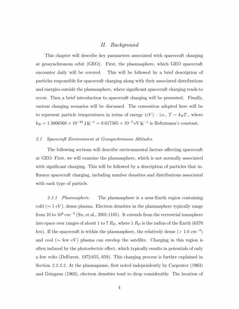
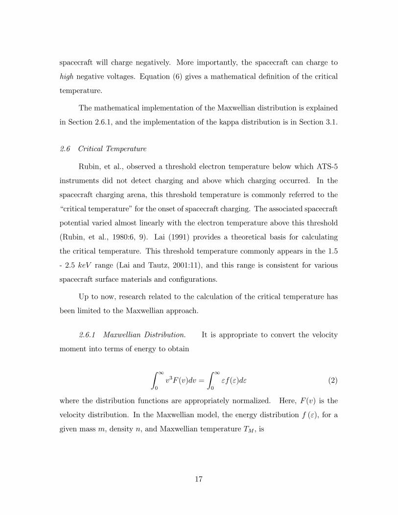
Figure 4, after Meyer-Vernet (1999:174), depicts the high-energy tail for κ = 3

and κ = 6 against a normalized velocity distribution, as in Equation (9). The

Maxwellian distribution, which corresponds to κ = ∞ (see Equation (10), for ex-

ample) is also plotted. Notice the similarity in the distributions for v ≤ w, whereasthe kappa distributions have an excess of high-speed particles not captured by the

Maxwellian distribution. The distributions are normalized so they have the same

number density and same most probable speed. Therefore, the low-energy distri-

20

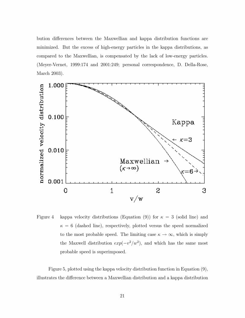
bution differences between the Maxwellian and kappa distribution functions are

minimized. But the excess of high-energy particles in the kappa distributions, as

compared to the Maxwellian, is compensated by the lack of low-energy particles.

(Meyer-Vernet, 1999:174 and 2001:249; personal correspondence, D. Della-Rose,

March 2003).

Figure 4 kappa velocity distributions (Equation (9)) for κ = 3 (solid line) and

κ = 6 (dashed line), respectively, plotted versus the speed normalized

to the most probable speed. The limiting case κ → ∞, which is simplythe Maxwell distribution exp(−v2/w2), and which has the same mostprobable speed is superimposed.

Figure 5, plotted using the kappa velocity distribution function in Equation (9),

illustrates the difference between a Maxwellian distribution and a kappa distribution

21

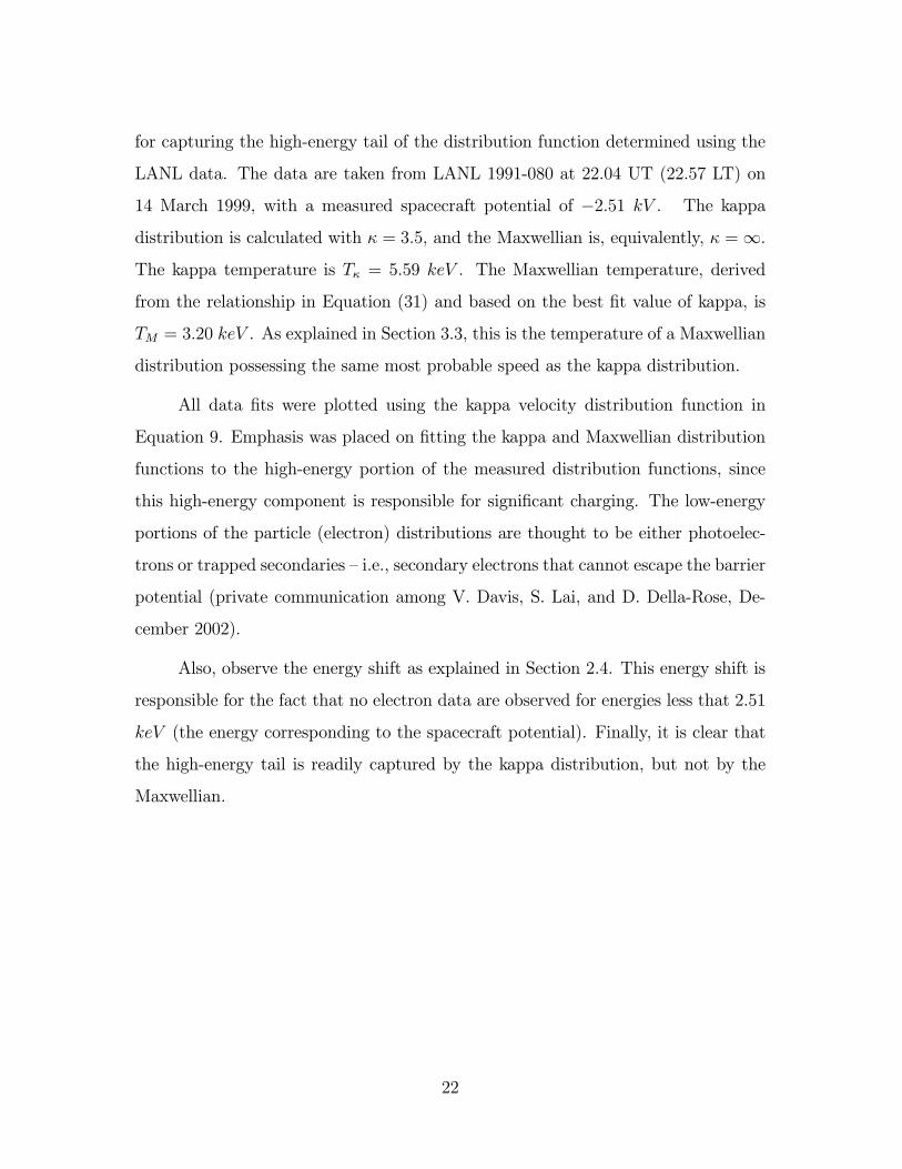
for capturing the high-energy tail of the distribution function determined using the

LANL data. The data are taken from LANL 1991-080 at 22.04 UT (22.57 LT) on

14 March 1999, with a measured spacecraft potential of −2.51 kV . The kappa

distribution is calculated with κ = 3.5, and the Maxwellian is, equivalently, κ =∞.The kappa temperature is Tκ = 5.59 keV . The Maxwellian temperature, derived

from the relationship in Equation (31) and based on the best fit value of kappa, is

TM = 3.20 keV . As explained in Section 3.3, this is the temperature of a Maxwellian

distribution possessing the same most probable speed as the kappa distribution.

All data fits were plotted using the kappa velocity distribution function in

Equation 9. Emphasis was placed on fitting the kappa and Maxwellian distribution

functions to the high-energy portion of the measured distribution functions, since

this high-energy component is responsible for significant charging. The low-energy

portions of the particle (electron) distributions are thought to be either photoelec-

trons or trapped secondaries — i.e., secondary electrons that cannot escape the barrier

potential (private communication among V. Davis, S. Lai, and D. Della-Rose, De-

cember 2002).

Also, observe the energy shift as explained in Section 2.4. This energy shift is

responsible for the fact that no electron data are observed for energies less that 2.51

keV (the energy corresponding to the spacecraft potential). Finally, it is clear that

the high-energy tail is readily captured by the kappa distribution, but not by the

Maxwellian.

22

0.01 0.1 1 10 1001 .10 35

1 .10 34

1 .10 33

1 .10 32

1 .10 31

1 .10 30

1 .10 29

1 .10 28

1 .10 27

1 .10 26

1 .10 25

1 .10 24

1 .10 23

Energy (keV)

Dis

tribu

tion

Func

tion

(sec

^3/c

m^6

)

κ 3.5= Tκ 5.59= keV

TM 3.20= keV

V 2.51−= kV Kp = 3 2/3

Figure 5 Electron Distribution Function vs. Electron Energy for LANL 1991-080

Data at 22.04 UT (22.57 LT) on 14 March 1999 Demonstrating Superior-

ity of the kappa Distribution over the Maxwellian at Capturing the High

Energy Tail. Plotted are LANL Data Values (circles), kappa Distribution

(solid), and Maxwellian Distribution (dash). (Data Courtesy of Michelle

F. Thomsen, Los Alamos National Laboratory.)

Vasyliunas was possibly the first to use the kappa distribution in its general

form and to note its relationship to the Maxwellian. He presents the kappa velocity

distribution as (Vasyliunas, 1968:2866-2867)

23

fκ(v) =n

(κw20)32

Γ (κ+ 1)

π32Γ¡κ− 1

2

¢ ·1 + v2

κw20

¸−(κ+1)(9)

where

n = the total number density

w0 = the most probable speed

κ = the exponent of the differential flux at high energies

That is, κ is really only of consequence in the high-energy portion of the dis-

tribution, since this part of the distribution is the basis for significant charging.

Vasyliunas notes appearances of kappa distributions, specifically with κ = 2, in ear-

lier literature (Vasyliunas, 1968:2866-2867; Summers and Thorne, 1991:1836). It is

the inverse power law relation

fκ(v) ∝·1 +

v2

κw20

¸−(κ+1)that is crucial to capturing the high-energy tail missed by the Maxwellian (Vasyliu-

nas, 1968:2866; Meyer-Vernet, 2001:248-249). Larger kappa values are more like the

Maxwellian, but the high-energy tail is captured by lower kappa values (Summers

and Thorne, 1991:1836). Here we also note that

limκ→∞

·1 +

v2

κw20

¸−(κ+1)= e

−mv2

2TM

= fM(v) (10)

which is the Maxwellian velocity distribution.

24

III. Approach

The approach taken for this research, which was geared toward suggestions

by Dr. Shu T. Lai of the Air Force Research Laboratory (personal correspondence

between S. Lai and D. Della-Rose, November 2001) was to first become familiar with

the Maxwellian theory which is presented in Section 2.6.1. This included a study

of the distribution function and the current balance equation using secondary and

backscattered coefficients. The next step was to become familiar with kappa theory

and understand its application to the high-energy tail in the electron distribution

functions. This was followed by formulation of the kappa current balance equation

with secondary and backscattered coefficients and deriving the analytical result.

Finally, comparison was made with the analytical results and observations.

3.1 Development of the Current Balance Equation Using the kappa Distribution

As in the Maxwellian model, we can define the kappa energy distribution func-

tion for a given mass m, density n, and (kappa) temperature Tκ (in energy units),

as

fκ(ε) = nAκ

µ2

κmw2

¶ 32

ε12

"1 +

ε¡κ− 3

2

¢Tκ

#−(κ+1)(11)

= nAκ

·µκ− 3

2

¶Tκ

¸− 32

ε12

"1 +

ε¡κ− 3

2

¢Tκ

#−(κ+1)(12)

where we note the requirement that κ > 3/2 and Aκ is the normalization factor

Aκ =Γ(κ+ 1)

Γ(32)Γ(κ− 1

2)

(13)

So the integral form of the current balance equation (with normalization terms can-

celled since they are not functions of ε) is then

25

Z ∞

0

ε

"1 +

ε¡κ− 3

2

¢Tκ

#−(κ+1)dε

=

Z ∞

0

ε

"1 +

ε¡κ− 3

2

¢Tκ

#−(κ+1)[c(e−

εa − e− ε

b ) +A−Be−εC ]dε (14)

Recall that this is an integration of the velocity moment as in Equation (2).

Originally, the integration was carried out in MATLABR°, which returned the

left-hand side of the equation as

Z ∞

0

ε

"1 +

ε¡κ− 3

2

¢Tκ

#−(κ+1)dε =

·(2κ− 3)Tκ2(κ− 1)

¸2(15)

but not in this simplified form, and MATLABR°returned the right-hand side as

Z ∞

0

ε

"1 +

ε¡κ− 3

2

¢Tκ

#−(κ+1)[c(e−

εa − e− ε

b ) +A−Be−εC ]dε

=(2κ− 3)Tκ2Γ(κ+ 1)

ca{Γ(κ− 1)(2κ− 3)Tκ2a

M

µ2, 2− κ,

(2κ− 3)Tκ2a

¶+π csc(πκ)κ

·(2κ− 3)Tκ

2a

¸κM

µκ+ 1,κ,

(2κ− 3)Tκ2a

¶}

−(2κ− 3)Tκ2Γ(κ+ 1)

cb{Γ(κ− 1)(2κ− 3)Tκ2b

M

µ2, 2− κ,

(2κ− 3)Tκ2b

¶+π csc(πκ)κ

·(2κ− 3)Tκ

2b

¸κM

µκ+ 1,κ,

(2κ− 3)Tκ2b

¶}

+

·(2κ− 3)Tκ2(κ− 1)

¸2A

−(2κ− 3)TκB2Γ(κ+ 1)C

{Γ(κ− 1)(2κ− 3)TκC2

M

µ2, 2− κ,

(2κ− 3)TκC2

¶+π csc(πκ)κ

·(2κ− 3)TκC

2

¸κM

µκ+ 1,κ,

(2κ− 3)TκC2

¶} (16)

26

which is likewise simplified from the original MATLABR°result for display here.

Dividing through by the left-hand side of Equation (14) and further simplifying

yields

c{Mµ2, 2− κ,

(2κ− 3)Tκ2a

¶+πκ csc(πκ)

Γ(κ− 1)·(2κ− 3)Tκ

2a

¸κ−1M

µκ+ 1,κ,

(2κ− 3)Tκ2a

¶−M

µ2, 2− κ,

(2κ− 3)Tκ2b

¶+πκ csc(πκ)

Γ(κ− 1)·(2κ− 3)Tκ

2b

¸κ−1M

µκ+ 1,κ,

(2κ− 3)Tκ2b

¶}

−B{Mµ2, 2− κ,

(2κ− 3)TκC2

¶+πκ csc(πκ)

Γ(κ− 1)·(2κ− 3)TκC

2

¸κ−1M

µκ+ 1,κ,

(2κ− 3)TκC2

¶}

+A− 1= 0 (17)

Now observe that

πκ csc(πκ)

Γ(κ− 1) =κ(−κ)Γ(−κ)Γ(κ)

Γ(κ− 1)= −Γ(κ+ 1)Γ(2− κ)

(κ− 1)Γ(κ− 1)= −Γ(κ+ 1)Γ(2− κ)

Γ(2)Γ(κ)(18)

since (Abramowitz and Stegun, 1965:256)

π csc(πκ) = (−κ)Γ(−κ)Γ(κ)

27

and

Γ(2) = 1

Now we note that

κ

Γ(κ− 1) = −Γ(κ+ 1)Γ(2− κ)

Γ(2)Γ(κ)

sinπκ

π(19)

= −Γ(κ+ 1)Γ(2− κ)

Γ(2)Γ(κ)

1

Γ(κ)Γ(1− κ)(20)

and consider

M (2, 2− κ, z) +πκ csc(πκ)

Γ(κ− 1) zκ−1M (κ+ 1,κ, z)

= M (2, 2− κ, z) +κ

Γ(κ− 1)π

sinπκzκ−1M (κ+ 1,κ, z)

= zκ−1π

sinπκ

½z1−κ

M (2, 2− κ, z)

π csc(πκ)+

κ

Γ(κ− 1)M (κ+ 1,κ, z)

¾= zκ−1

π

sinπκ

½z1−κ

M (2, 2− κ, z)

Γ(κ)Γ(1− κ)− Γ(κ+ 1)Γ(2− κ)

Γ(2)Γ(κ)

M (κ+ 1,κ, z)

Γ(κ)Γ(1− κ)

¾= zκ−1κ (κ− 1) π

sinπκ

½M (κ+ 1,κ, z)

Γ(2)Γ(κ)− z1−κ M (2, 2− κ, z)

Γ(κ+ 1)Γ(2− κ)

¾(21)

= zκ−1κ (κ− 1) π

sinπb

½M (a, b, z)

Γ(1 + a− b)Γ(b) − z1−bM (1 + a− b, 2− b, z)

Γ(a)Γ(2− b)¾

= zκ−1κ (κ− 1)U (a, b, z) (22)

where we let a = κ + 1 and b = κ, corresponding to the definition of Kummer’s

function (Abramowitz and Stegun, 1965:504),

M(a, b, z) = 1 +az

b+(a)2z

2

(b)22!+ · · ·+ (a)nz

n

(b)nn!+ · · ·

where

28

(a)n = a(a+ 1)(a+ 2) . . . (a+ n− 1)(a)0 = 1

and

U(a, b, z) =π

sinπb

·M(a, b, z)

Γ(1 + a− b)Γ(b) − z1−bM(1 + a− b, 2− b, z)

Γ(a)Γ(2− b)¸

This leads to our initial result for the kappa current balance equation:

κ (κ− 1)·(2κ− 3)Tκ

2

¸κ−1{ca1−κU

µκ+ 1,κ,

(2κ− 3)Tκ2a

¶−cb1−κU

µκ+ 1,κ,

(2κ− 3)Tκ2b

¶−BCκ−1U

µκ+ 1,κ,

(2κ− 3)TκC2

¶}

+A− 1= 0 (23)

The solution Tκ of this equation is the critical (kappa) temperature for charging

onset for a given material and value of kappa. For reference, a table of critical

temperatures calculated for non-activated CuBe over a range of values, κ = 2.5 to

17.5, is available in Appendix D.

However, a more direct approach is the Whittaker function (Appendix B). The

practical application of the Whittaker function came to light long after the initial

analysis of the current balance equation was complete. The graphs of the two are

(theoretically) identical, but the Whittaker function converges more quickly to the

Maxwellian possibly since there is less error propagation due to round-off in the

numerical calculations.

29

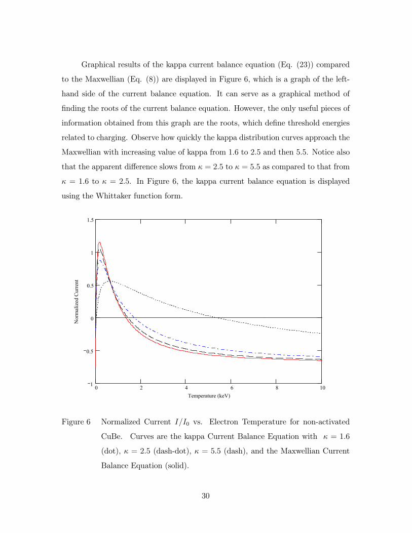
Graphical results of the kappa current balance equation (Eq. (23)) compared

to the Maxwellian (Eq. (8)) are displayed in Figure 6, which is a graph of the left-

hand side of the current balance equation. It can serve as a graphical method of

finding the roots of the current balance equation. However, the only useful pieces of

information obtained from this graph are the roots, which define threshold energies

related to charging. Observe how quickly the kappa distribution curves approach the

Maxwellian with increasing value of kappa from 1.6 to 2.5 and then 5.5. Notice also

that the apparent difference slows from κ = 2.5 to κ = 5.5 as compared to that from

κ = 1.6 to κ = 2.5. In Figure 6, the kappa current balance equation is displayed

using the Whittaker function form.

0 2 4 6 8 101

0.5

0

0.5

1

1.5

Temperature (keV)

Nor

mal

ized

Cur

rent

Figure 6 Normalized Current I/I0 vs. Electron Temperature for non-activated

CuBe. Curves are the kappa Current Balance Equation with κ = 1.6

(dot), κ = 2.5 (dash-dot), κ = 5.5 (dash), and the Maxwellian Current

Balance Equation (solid).

30

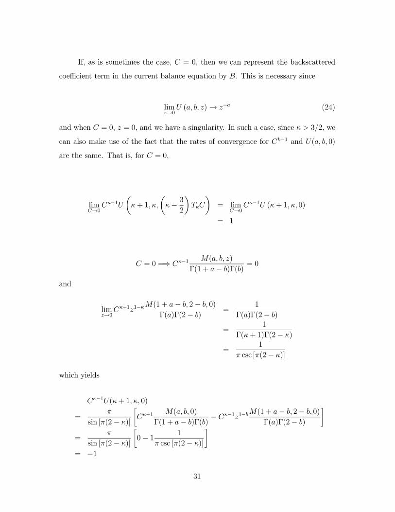
If, as is sometimes the case, C = 0, then we can represent the backscattered

coefficient term in the current balance equation by B. This is necessary since

limz→0

U (a, b, z)→ z−a (24)

and when C = 0, z = 0, and we have a singularity. In such a case, since κ > 3/2, we

can also make use of the fact that the rates of convergence for Ck−1 and U(a, b, 0)

are the same. That is, for C = 0,

limC→0

Cκ−1Uµκ+ 1,κ,

µκ− 3

2

¶TκC

¶= lim

C→0Cκ−1U (κ+ 1,κ, 0)

= 1

C = 0 =⇒ Cκ−1 M(a, b, z)

Γ(1 + a− b)Γ(b) = 0

and

limz→0

Cκ−1z1−κM(1 + a− b, 2− b, 0)

Γ(a)Γ(2− b) =1

Γ(a)Γ(2− b)=

1

Γ(κ+ 1)Γ(2− κ)

=1

π csc [π(2− κ)]

which yields

Cκ−1U(κ+ 1,κ, 0)

=π

sin [π(2− κ)]

·Cκ−1 M(a, b, 0)

Γ(1 + a− b)Γ(b) − Cκ−1z1−b

M(1 + a− b, 2− b, 0)Γ(a)Γ(2− b)

¸=

π

sin [π(2− κ)]

·0− 1 1

π csc [π(2− κ)]

¸= −1

31

and the last term in the current balance equation takes on the value of B (private

communication, Aihua W. Wood, December 2002). As in the case of the Kummer

form of the current balance equation, we can set the backscattered coefficient term

in the Whittaker form to B when C = 0. Figure 7 is a graph of the normalized

current vs. temperature for kapton — a material for which C = 0.

0 2 4 6 8 101

0.5

0

0.5

1

1.5

Temperature (keV)

Nor

mal

ized

Cur

rent

Figure 7 Normalized Current I/I0 vs. Electron Temperature for kapton. Curves

are the kappa Current Balance Equation with κ = 1.6 (dot), κ = 2.5

(dash-dot), κ = 5.5 (dash), and the Maxwellian Current Balance Equa-

tion (solid).

3.2 Data Selection and Acquisition

Following the determination of the dates of interest for comparison to data

analyzed by Lai and Della-Rose (2001), the data were made available for ftp acqui-

sition by the Los Alamos National Laboratory. The data were then converted into

32

a useable format for graphical analysis in Mathcad R°. However, the LANL dataobtained covered only a subset of the cases examined in Lai and Della-Rose (2001),

so emphasis was placed on eclipse charging events occurring in March 1999. Data

for April 1999, and June 2000 were also examined for significant (potential > 1 kV )

spacecraft charging events.

Data measurements were taken by magnetospheric plasma analyzers (MPAs)

deployed on a number of Department of Energy GEO satellites. The purpose of

the MPAs is to monitor the three-dimensional plasma electron and ion distributions

at GEO in support of the spacecraft mission (Thomsen, et al., 1999:1). The data

studied were angle-averaged from the full three-dimensional distribution, which is

obtained in one approximately 10-second satellite spin (Thomsen, et al., 1999:1).

The charging events selected include the following associated data used in this

study:

Date-time group (UT and spacecraft LT), spacecraft geographic coordinates

(km - discussed in Appendix A), spacecraft potential (V ), IP flags, electron density

(#/cm−3), parallel and perpendicular hot electron temperatures, and differential

particle fluxes in each of 40 channels. IP flags signify whether an ion line was found

or an iteration procedure was used to determine the spacecraft potential. The use of

ion lines to determine spacecraft potential is generally considered reliable (Thomsen,

et al., 1999:11-13). Based on a graphical comparison of data for ion lines found vs.

iteration, iteration data also appeared reliable.

The particle fluxes in the data were measured at the instrument, but were not

corrected for spacecraft potential (personal correspondence between M. Thomsen

and D. Della-Rose, October 2002). The temperatures are experimentally derived

using

33

T =1

n

Zm (v−V) (v−V) f(v)d3v (25)

=1

n

Zm (vv) f(v)d3v−mVV (26)

where v is the total velocity, V is the average velocity of the electrons in the plasma,

and f(v) is the measured phase space density as a function of v. The distribution

function based on channel energy data is determined by multiplying the differential

flux F (cm−2 s−1 sr−1 eV −1) by Ke and dividing this product by the center energy

Ec (eV ) for that channel (Thomsen, et al., 1999:2, 14-15, 18-19). That is,

fdatai =FiKe

Eci(27)

where i is the channel number (1-40) and

Ke =m2e

2= 1.616× 10−31eV 2cm−4s4 (28)

3.3 Method of Analysis

Three distribution functions were plotted against the channel center energies

on a log-log plot and visually analyzed. The distribution functions examined were

from the LANL data, the kappa distribution, and the Maxwellian distribution. Vi-

sual fitting was utilized because the numerical routines for fitting failed to achieve

reasonable results. Though the distribution functions averaged out in the numerical

routines, the averages resulted from large deviations above and below the measured

distributions (i.e., the fits were clearly poor).

All data fits were plotted using the kappa velocity distribution function in

Equation (9). Emphasis was placed on fitting the kappa and Maxwellian distribution

functions to the high-energy portion of the measured distribution functions, since

34

this high-energy component is responsible for significant charging. The low-energy

portions of the particle (electron) distributions are thought to be either photoelec-

trons or trapped secondaries (i.e., secondary electrons that cannot escape the barrier

potential), as opposed to being part of the ambient plasma.

The channel center energies are calculated by taking the geometric mean of

the (corrected) edge energies Ed for each channel. The corrected energy of a particle

(based on the energy shift as explained in Section 2.4) can be represented by taking

the energy at infinity E0 and subtracting the spacecraft potential, i.e., (Thomsen, et

al., 1999:14)

E = E0 − qVsc (29)

The distribution function graphs were then examined to visually fit a kappa

value to the high-energy, non-Maxwellian tails of the plots. Observe that on the

log-log plots, since

log

"1 +

ε¡κ− 3

2

¢Tκ

#−(κ+1)= −(κ+ 1) log

"1 +

ε¡κ− 3

2

¢Tκ

#(30)

the kappa values determined the slopes of the curves when the second term in the

argument of the logarithm is much greater than 1. Next, the kappa temperature

was varied until a fit was achieved. This kappa temperature was converted to a

Maxwellian representation by using the temperature conversion

TM =

¡κ− 3

2

¢κ

Tκ (31)

where Tκ is derived by computing12m hv2i (i.e., the average kinetic energy) for the

kappa distribution and equating it to 32Tκ. The relationship between TM and Tκ

follows from the fact that the most probable speed, w0, is independent of kappa

35

and from the relationship in Equation (10) (personal communication, D. Della-Rose,

February 2003). Notice that

limκ→∞

κ− 32

κTκ = TM (32)

The Maxwellian temperature was then input into a Maxwellian distribution

and plotted.

In addition to a visual inspection for curve fitting, electron number densities for

the range of channels that correlated to a good visual fit were computed. The number

densities for the data were used as a basis for comparison. This technique aided in

refining the fit by eliminating some of the subjectivity, especially when a range of

temperatures seemed to provide a good kappa fit. The temperature that returned the

nearest kappa distribution number density compared to the measured data number

density was used. The equations for data number density, kappa number density

and Maxwellian number density were, respectively,

ndata = 4π

µ2

me

¶ 32highXk=low

Eck

³qEdk−1 + qVsc −

pEdk + qVsc

´fdatak (33)

nκ (κ, Tκ) = 2nheAκ

·µκ− 3

2

¶Tκ

¸− 32

highXk=low

Eck


pEdk + qVsc

´"1 +

Eck¡κ− 3

2

¢Tκ

#−(κ+1)(34)

36

nM (TM) = 4π

µ1

πTM

¶ 32

nhe

highXk=low

Eck


pEdk + qVsc

´e(−Eck

TM)

(35)

where low is the lowest channel number (corresponding to highest energy channel),

and high is the highest channel number fitted, q is the charge on the particle of

interest (electron), and Ec and Ed are the corrected channel center energy and un-

corrected channel edge energy, respectively. For example, consider Figure 8 where

channels 1-7 are fit well with the kappa curve. Note, too, that nκ and nM are func-

tions of nhe, the hot electron number density provided in the LANL data. A partial

table of (uncorrected) channel energies is available in Appendix C.

Figures 8 and 9 show the electron distribution function vs. electron energy for

09 March 1999 at 16.67 UT (23.57 LT) and 16.79 UT (23.69 LT), respectively, for

LANL 1994-084 data. The time in Figure 8 is about 8 minutes before the satellite

enters eclipse and near the onset of a period of charging. In this figure, κ = 5.5,

the kappa temperature from the fitting procedure is Tκ = 1.43 keV , the Maxwellian

temperature is TM = 1.04 keV , and the spacecraft potential is V = −22 V . Thegeomagnetic index was Kp = 3

13during this time frame.

37

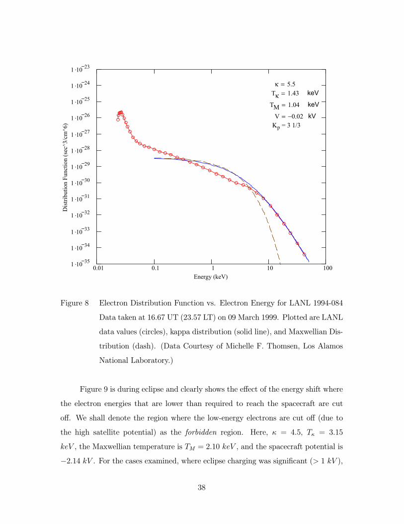
0.01 0.1 1 10 1001 .10 35

1 .10 34

1 .10 33

1 .10 32

1 .10 31

1 .10 30

1 .10 29

1 .10 28

1 .10 27

1 .10 26

1 .10 25

1 .10 24

1 .10 23

Energy (keV)

Dis

tribu

tion

Func

tion

(sec

^3/c

m^6

)

κ 5.5= Tκ 1.43= keV

TM 1.04= keV

V 0.02−= kV Kp = 3 1/3

Figure 8 Electron Distribution Function vs. Electron Energy for LANL 1994-084

Data taken at 16.67 UT (23.57 LT) on 09 March 1999. Plotted are LANL

data values (circles), kappa distribution (solid line), and Maxwellian Dis-

tribution (dash). (Data Courtesy of Michelle F. Thomsen, Los Alamos

National Laboratory.)

Figure 9 is during eclipse and clearly shows the effect of the energy shift where

the electron energies that are lower than required to reach the spacecraft are cut

off. We shall denote the region where the low-energy electrons are cut off (due to

the high satellite potential) as the forbidden region. Here, κ = 4.5, Tκ = 3.15

keV , the Maxwellian temperature is TM = 2.10 keV , and the spacecraft potential is

−2.14 kV . For the cases examined, where eclipse charging was significant (> 1 kV ),

38

charging normally began as eclipse approached, and the potential tended to reach

the maximum values for the day during eclipse.

0.01 0.1 1 10 1001 .10 35

1 .10 34

1 .10 33

1 .10 32

1 .10 31

1 .10 30

1 .10 29

1 .10 28

1 .10 27

1 .10 26

1 .10 25

1 .10 24

1 .10 23

Energy (keV)

Dis

tribu

tion

Func

tion

(sec

^3/c

m^6

)

κ 4.5= Tκ 3.15= keV

TM 2.10= keV

V 2.14−= kV Kp = 3 1/3

Figure 9 Electron Distribution Function vs. Electron Energies for LANL 1994-084

Data taken at 16.79 UT (23.69 LT) on 09 March 1999. Plotted are LANL

data values (circles), kappa distribution (solid line), and Maxwellian Dis-

tribution (dash). (Data Courtesy of Michelle F. Thomsen, Los Alamos


39

IV. Analysis

This chapter presents an examination of an eclipse charging event which took place

during one of the periods examined by Lai and Della-Rose (2001). This event was

chosen since it is representative of significant charging that can occur during eclipse,

and the pattern of charging is consistent with other charging events of this type in

the data we examined. The data presented will provide a basis for evaluating the

value of the kappa distribution, as compared to the Maxwellian distribution, as a

predictor of the onset of significant spacecraft charging.

As noted in Section 3.3, in the interest of minimizing subjectivity, electron

number densities were calculated for use in conjunction with visual fits. The num-

ber densities were calculated from Equations (33), (34), and (35). These number

densities were used to help narrow down the best temperature fit corresponding to

the chosen kappa value. The kappa value was selected based on its sufficiency for

modeling the slope of the high-energy part of a given particle distribution.

4.1 Principal Features of Concern

As the electron energy distribution shifts to higher energies, the slope of the tail

with energies > 10 keV decreases, indicating that smaller kappa values are associated

with more high-energy electrons. These low kappa values are positively correlated

to higher potentials, as expected. This follows since, for incident electrons in region

III of the secondary emission curve, a large potential must develop before a balance

between incoming and outgoing currents will be achieved, resulting in a steady-state

potential. Conversely, large kappa values tend to signify lower distributions of high-

energy electrons, resulting in lower spacecraft potentials. This is evident in Figures

8 and 9, and it is consistent with the explanation given by Hastings and Garrett

(1996:70). These incident, high-energy electrons characterized by the tail continue

to increase the spacecraft surface potential until a steady-state potential is reached.

40

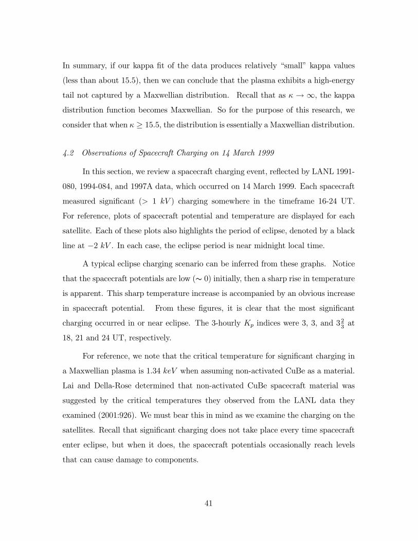
In summary, if our kappa fit of the data produces relatively “small” kappa values

(less than about 15.5), then we can conclude that the plasma exhibits a high-energy

tail not captured by a Maxwellian distribution. Recall that as κ → ∞, the kappadistribution function becomes Maxwellian. So for the purpose of this research, we

consider that when κ ≥ 15.5, the distribution is essentially a Maxwellian distribution.

4.2 Observations of Spacecraft Charging on 14 March 1999

In this section, we review a spacecraft charging event, reflected by LANL 1991-

080, 1994-084, and 1997A data, which occurred on 14 March 1999. Each spacecraft

measured significant (> 1 kV ) charging somewhere in the timeframe 16-24 UT.

For reference, plots of spacecraft potential and temperature are displayed for each

satellite. Each of these plots also highlights the period of eclipse, denoted by a black

line at −2 kV . In each case, the eclipse period is near midnight local time.

A typical eclipse charging scenario can be inferred from these graphs. Notice

that the spacecraft potentials are low (∼ 0) initially, then a sharp rise in temperature

is apparent. This sharp temperature increase is accompanied by an obvious increase

in spacecraft potential. From these figures, it is clear that the most significant

charging occurred in or near eclipse. The 3-hourly Kp indices were 3, 3, and 323at

18, 21 and 24 UT, respectively.

For reference, we note that the critical temperature for significant charging in

a Maxwellian plasma is 1.34 keV when assuming non-activated CuBe as a material.

Lai and Della-Rose determined that non-activated CuBe spacecraft material was

suggested by the critical temperatures they observed from the LANL data they

examined (2001:926). We must bear this in mind as we examine the charging on the

satellites. Recall that significant charging does not take place every time spacecraft

enter eclipse, but when it does, the spacecraft potentials occasionally reach levels

that can cause damage to components.

41

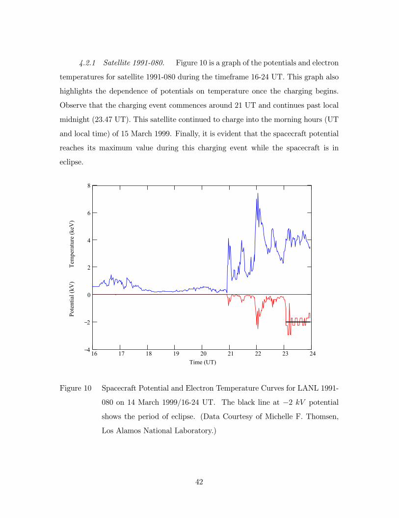
4.2.1 Satellite 1991-080. Figure 10 is a graph of the potentials and electron

temperatures for satellite 1991-080 during the timeframe 16-24 UT. This graph also

highlights the dependence of potentials on temperature once the charging begins.

Observe that the charging event commences around 21 UT and continues past local

midnight (23.47 UT). This satellite continued to charge into the morning hours (UT

and local time) of 15 March 1999. Finally, it is evident that the spacecraft potential

reaches its maximum value during this charging event while the spacecraft is in

eclipse.

16 17 18 19 20 21 22 23 244

2

0

2

4

6

8

Time (UT)

Pote

ntia

l (kV

)

T

empe

ratu

re (k

eV)

Figure 10 Spacecraft Potential and Electron Temperature Curves for LANL 1991-

080 on 14 March 1999/16-24 UT. The black line at −2 kV potential

shows the period of eclipse. (Data Courtesy of Michelle F. Thomsen,

Los Alamos National Laboratory.)

42

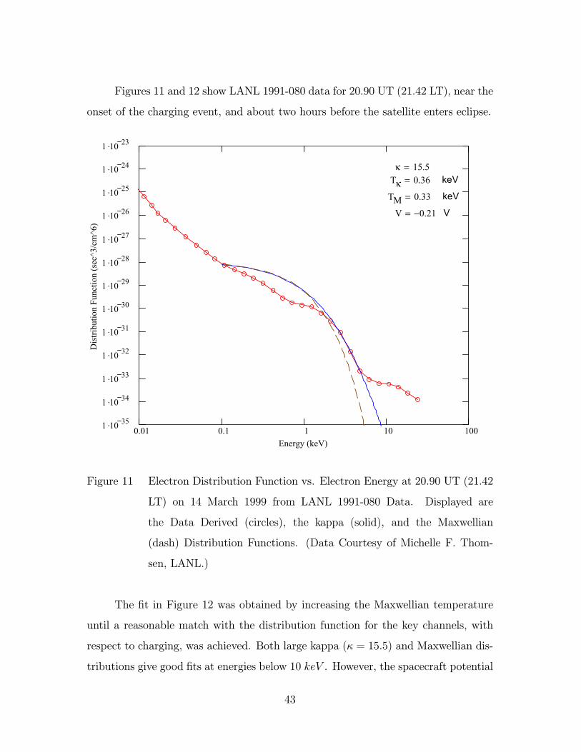
Figures 11 and 12 show LANL 1991-080 data for 20.90 UT (21.42 LT), near the

onset of the charging event, and about two hours before the satellite enters eclipse.

0.01 0.1 1 10 1001 .10 35

1 .10 34

1 .10 33

1 .10 32

1 .10 31

1 .10 30

1 .10 29

1 .10 28

1 .10 27

1 .10 26

1 .10 25

1 .10 24

1 .10 23

Energy (keV)

Dis

tribu

tion

Func

tion

(sec

^3/c

m^6

)

κ 15.5= Tκ 0.36= keV

TM 0.33= keV

V 0.21−= V

Figure 11 Electron Distribution Function vs. Electron Energy at 20.90 UT (21.42



(dash) Distribution Functions. (Data Courtesy of Michelle F. Thom-

sen, LANL.)

The fit in Figure 12 was obtained by increasing the Maxwellian temperature

until a reasonable match with the distribution function for the key channels, with

respect to charging, was achieved. Both large kappa (κ = 15.5) and Maxwellian dis-

tributions give good fits at energies below 10 keV . However, the spacecraft potential

43

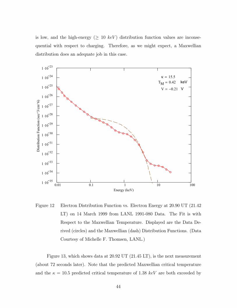
is low, and the high-energy (≥ 10 keV ) distribution function values are inconse-

quential with respect to charging. Therefore, as we might expect, a Maxwellian

distribution does an adequate job in this case.

0.01 0.1 1 10 1001 .10 35

1 .10 34

1 .10 33

1 .10 32

1 .10 31

1 .10 30

1 .10 29

1 .10 28

1 .10 27

1 .10 26

1 .10 25

1 .10 24

1 .10 23

Energy (keV)

Dis

tribu

tion

Func

tion

(sec

^3/c

m^6

)

κ 15.5=TM 0.42= keV

V 0.21−= V


LT) on 14 March 1999 from LANL 1991-080 Data. The Fit is with

Respect to the Maxwellian Temperature. Displayed are the Data De-

rived (circles) and the Maxwellian (dash) Distribution Functions. (Data

Courtesy of Michelle F. Thomsen, LANL.)

Figure 13, which shows data at 20.92 UT (21.45 LT), is the next measurement

(about 72 seconds later). Note that the predicted Maxwellian critical temperature

and the κ = 10.5 predicted critical temperature of 1.38 keV are both exceeded by

44

the fitted kappa temperature. This is consistent with the theory that significant

charging can occur above the critical temperature. One key feature of this graph is

that the kappa fit is noticeably better than the Maxwellian fit in the high-energy part

of the distribution, even if the Maxwellian temperature is increased. This graph, and

those with potentials larger than about 20 eV that follow, are solid examples of the

energy shift described in Section 3.3. The correlation between this energy shift, qV ,

and the associated spacecraft potential, V , stands out in each case.

0.01 0.1 1 10 1001 .10 35

1 .10 34

1 .10 33

1 .10 32

1 .10 31

1 .10 30

1 .10 29

1 .10 28

1 .10 27

1 .10 26

1 .10 25

1 .10 24

1 .10 23

Energy (keV)

Dis

tribu

tion

Func

tion

(sec

^3/c

m^6

)

κ 10.5= Tκ 2.44= keV

TM 2.09= keV

V 0.20−= kV


LT) on 14 March 1999 from LANL 1991-080 Data. Displayed are the

Data Derived (circles), the kappa (solid), and the Maxwellian (dash)

Distribution Functions. (Data Courtesy of Michelle F. Thomsen, Los

Alamos National Laboratory.)

45

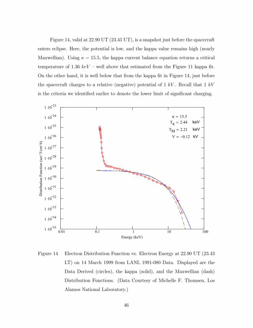
Figure 14, valid at 22.90 UT (23.45 UT), is a snapshot just before the spacecraft

enters eclipse. Here, the potential is low, and the kappa value remains high (nearly

Maxwellian). Using κ = 15.5, the kappa current balance equation returns a critical

temperature of 1.36 keV — well above that estimated from the Figure 11 kappa fit.

On the other hand, it is well below that from the kappa fit in Figure 14, just before

the spacecraft charges to a relative (negative) potential of 1 kV . Recall that 1 kV

is the criteria we identified earlier to denote the lower limit of significant charging.

0.01 0.1 1 10 1001 .10 35

1 .10 34

1 .10 33

1 .10 32

1 .10 31

1 .10 30

1 .10 29

1 .10 28

1 .10 27

1 .10 26

1 .10 25

1 .10 24

1 .10 23

Energy (keV)

Dis

tribu

tion

Func

tion

(sec

^3/c

m^6

)

κ 15.5= Tκ 2.44= keV

TM 2.21= keV

V 0.12−= kV






46

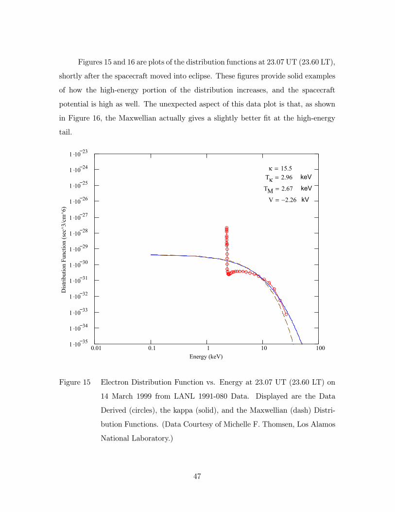
Figures 15 and 16 are plots of the distribution functions at 23.07 UT (23.60 LT),

shortly after the spacecraft moved into eclipse. These figures provide solid examples

of how the high-energy portion of the distribution increases, and the spacecraft

potential is high as well. The unexpected aspect of this data plot is that, as shown

in Figure 16, the Maxwellian actually gives a slightly better fit at the high-energy

tail.

0.01 0.1 1 10 1001 .10 35

1 .10 34

1 .10 33

1 .10 32

1 .10 31

1 .10 30

1 .10 29

1 .10 28

1 .10 27

1 .10 26

1 .10 25

1 .10 24

1 .10 23

Energy (keV)

Dis

tribu

tion

Func

tion

(sec

^3/c

m^6

)

κ 15.5= Tκ 2.96= keV

TM 2.67= keV

V 2.26−= kV

Figure 15 Electron Distribution Function vs. Energy at 23.07 UT (23.60 LT) on

14 March 1999 from LANL 1991-080 Data. Displayed are the Data

Derived (circles), the kappa (solid), and the Maxwellian (dash) Distri-

bution Functions. (Data Courtesy of Michelle F. Thomsen, Los Alamos


47

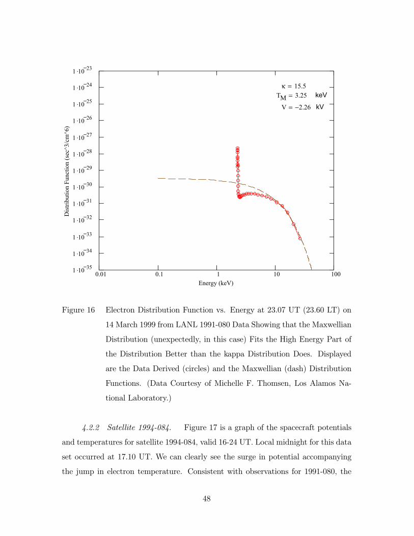
0.01 0.1 1 10 1001 .10 35

1 .10 34

1 .10 33

1 .10 32

1 .10 31

1 .10 30

1 .10 29

1 .10 28

1 .10 27

1 .10 26

1 .10 25

1 .10 24

1 .10 23

Energy (keV)

Dis

tribu

tion

Func

tion

(sec

^3/c

m^6

)

κ 15.5=TM 3.25= keV

V 2.26−= kV


14 March 1999 from LANL 1991-080 Data Showing that the Maxwellian

Distribution (unexpectedly, in this case) Fits the High Energy Part of

the Distribution Better than the kappa Distribution Does. Displayed

are the Data Derived (circles) and the Maxwellian (dash) Distribution

Functions. (Data Courtesy of Michelle F. Thomsen, Los Alamos Na-

tional Laboratory.)

4.2.2 Satellite 1994-084. Figure 17 is a graph of the spacecraft potentials

and temperatures for satellite 1994-084, valid 16-24 UT. Local midnight for this data

set occurred at 17.10 UT. We can clearly see the surge in potential accompanying

the jump in electron temperature. Consistent with observations for 1991-080, the

48

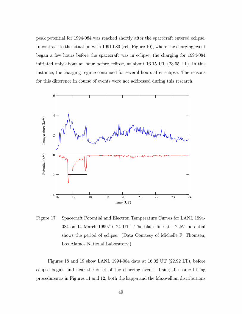
peak potential for 1994-084 was reached shortly after the spacecraft entered eclipse.

In contrast to the situation with 1991-080 (ref. Figure 10), where the charging event

began a few hours before the spacecraft was in eclipse, the charging for 1994-084

initiated only about an hour before eclipse, at about 16.15 UT (23.05 LT). In this

instance, the charging regime continued for several hours after eclipse. The reasons

for this difference in course of events were not addressed during this research.

16 17 18 19 20 21 22 23 244

2

0

2

4

6

Time (UT)

Pote

ntia

l (kV

)

T

empe

ratu

re (k

eV)

Figure 17 Spacecraft Potential and Electron Temperature Curves for LANL 1994-

084 on 14 March 1999/16-24 UT. The black line at −2 kV potential

shows the period of eclipse. (Data Courtesy of Michelle F. Thomsen,

Los Alamos National Laboratory.)

Figures 18 and 19 show LANL 1994-084 data at 16.02 UT (22.92 LT), before

eclipse begins and near the onset of the charging event. Using the same fitting

procedures as in Figures 11 and 12, both the kappa and the Maxwellian distributions

49

give good fits at energies below 10 keV , but the kappa fit in Figure 18 is clearly

superior overall in this case. This result contrasts with that for the first data plots

of satellite 1991-080.

0.01 0.1 1 10 1001 .10 35

1 .10 34

1 .10 33

1 .10 32

1 .10 31

1 .10 30

1 .10 29

1 .10 28

1 .10 27

1 .10 26

1 .10 25

1 .10 24

1 .10 23

Energy (keV)

Dis

tribu

tion

Func

tion

(sec

^3/c

m^6

)

κ 10.5= Tκ 0.71= keV

TM 0.61= keV

V 3.30−= V


14 March 1999 from LANL Satellite 1994-084 Data. Displayed are the




50

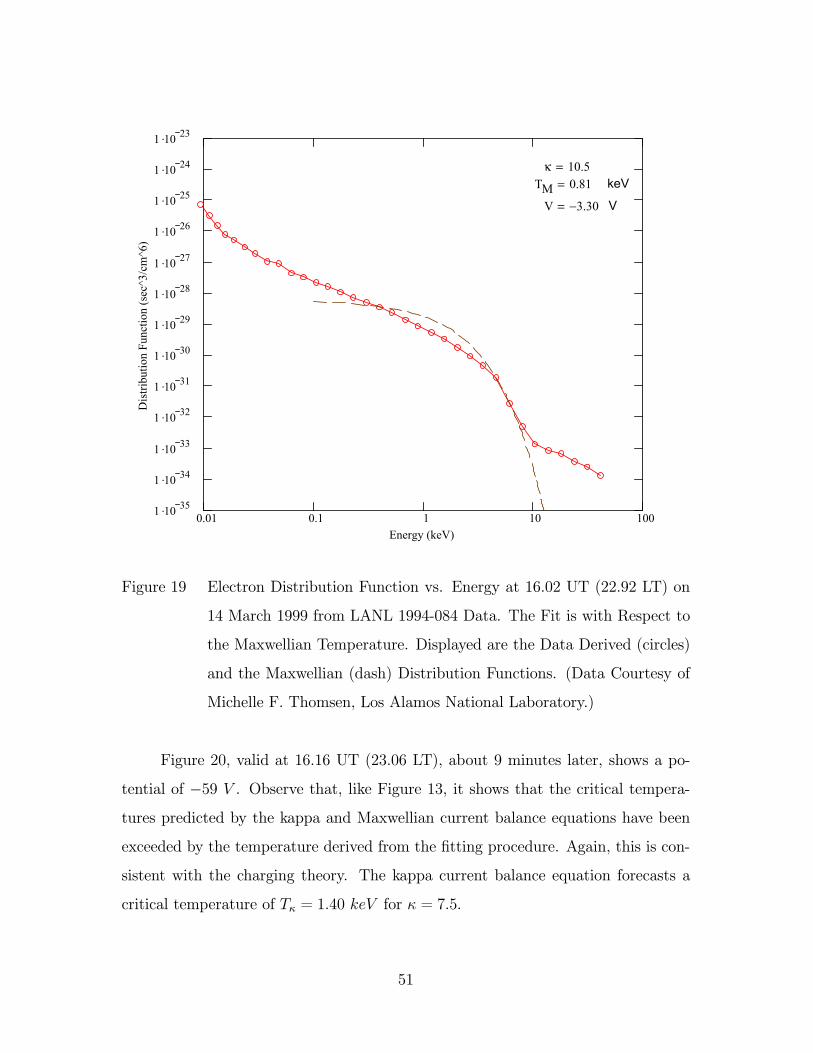
0.01 0.1 1 10 1001 .10 35

1 .10 34

1 .10 33

1 .10 32

1 .10 31

1 .10 30

1 .10 29

1 .10 28

1 .10 27

1 .10 26

1 .10 25

1 .10 24

1 .10 23

Energy (keV)

Dis

tribu

tion

Func

tion

(sec

^3/c

m^6

)

κ 10.5=TM 0.81= keV

V 3.30−= V


14 March 1999 from LANL 1994-084 Data. The Fit is with Respect to

the Maxwellian Temperature. Displayed are the Data Derived (circles)

and the Maxwellian (dash) Distribution Functions. (Data Courtesy of


Figure 20, valid at 16.16 UT (23.06 LT), about 9 minutes later, shows a po-

tential of −59 V . Observe that, like Figure 13, it shows that the critical tempera-tures predicted by the kappa and Maxwellian current balance equations have been

exceeded by the temperature derived from the fitting procedure. Again, this is con-

sistent with the charging theory. The kappa current balance equation forecasts a

critical temperature of Tκ = 1.40 keV for κ = 7.5.

51

A notable feature of the next three data plots, including Figure 20, is that the

kappa distribution clearly does a superior job of representing the measured distribu-

tion functions. Notice how the slope of the high-energy data is picked up by the kappa

distribution in all cases. Moreover, as the potential increases, the slope decreases,

and the kappa values follow suit. Even the low voltage case was better depicted by

the kappa curves than by the Maxwellian. This fact sets these measurements apart

from those on the other two spacecraft.

0.01 0.1 1 10 1001 .10 35

1 .10 34

1 .10 33

1 .10 32

1 .10 31

1 .10 30

1 .10 29

1 .10 28

1 .10 27

1 .10 26

1 .10 25

1 .10 24

1 .10 23

Energy (keV)

Dis

tribu

tion

Func

tion

(sec

^3/c

m^6

)

κ 7.5= Tκ 1.75= keV

TM 1.40= keV

V 0.06−= kV






52

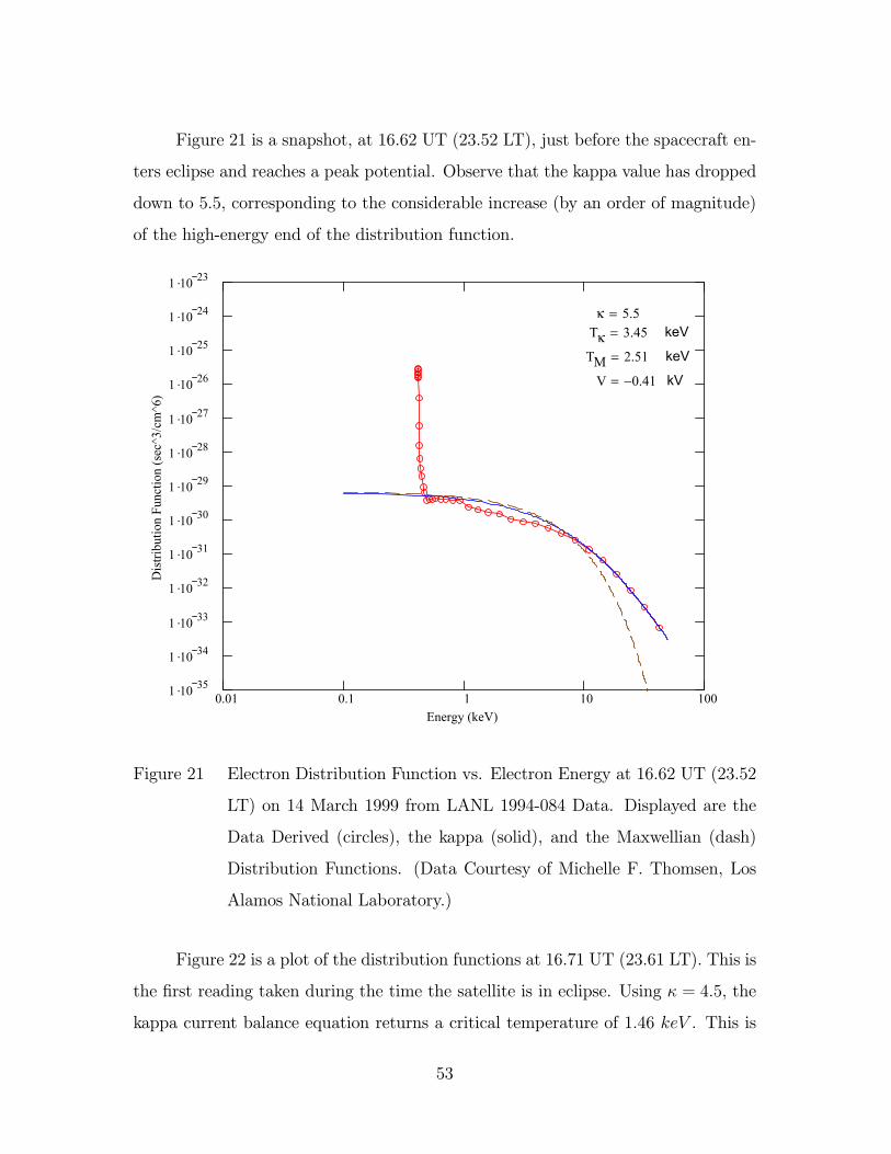
Figure 21 is a snapshot, at 16.62 UT (23.52 LT), just before the spacecraft en-

ters eclipse and reaches a peak potential. Observe that the kappa value has dropped

down to 5.5, corresponding to the considerable increase (by an order of magnitude)

of the high-energy end of the distribution function.

0.01 0.1 1 10 1001 .10 35

1 .10 34

1 .10 33

1 .10 32

1 .10 31

1 .10 30

1 .10 29

1 .10 28

1 .10 27

1 .10 26

1 .10 25

1 .10 24

1 .10 23

Energy (keV)

Dis

tribu

tion

Func

tion

(sec

^3/c

m^6

)

κ 5.5= Tκ 3.45= keV

TM 2.51= keV

V 0.41−= kV






Figure 22 is a plot of the distribution functions at 16.71 UT (23.61 LT). This is

the first reading taken during the time the satellite is in eclipse. Using κ = 4.5, the

kappa current balance equation returns a critical temperature of 1.46 keV . This is

53

far below the corresponding temperatures that make the curves fit well for Figures

21 and 22. This contrasts with using κ = 10.5 in Figure 18, which returns a critical

temperature of 1.38 keV — well above that which produced a good fit at that time.

0.01 0.1 1 10 1001 .10 35

1 .10 34

1 .10 33

1 .10 32

1 .10 31

1 .10 30

1 .10 29

1 .10 28

1 .10 27

1 .10 26

1 .10 25

1 .10 24

1 .10 23

Energy (keV)

Dis

tribu

tion

Func

tion

(sec

^3/c

m^6

)

κ 4.5= Tκ 2.78= keV

TM 1.85= keV

V 2.80−= kV


14 March 1999 from LANL 1994-084 Data. Displayed are the Data




4.2.3 Satellite 1997A. Finally, we examine LANL 1997A data. One clear

difference between this and the other spacecraft is that 1997A underwent significant

charging in the middle of the period 16-24 UT. Notice that charging began almost

three hours before the satellite migrated into eclipse, and the event continued for

54

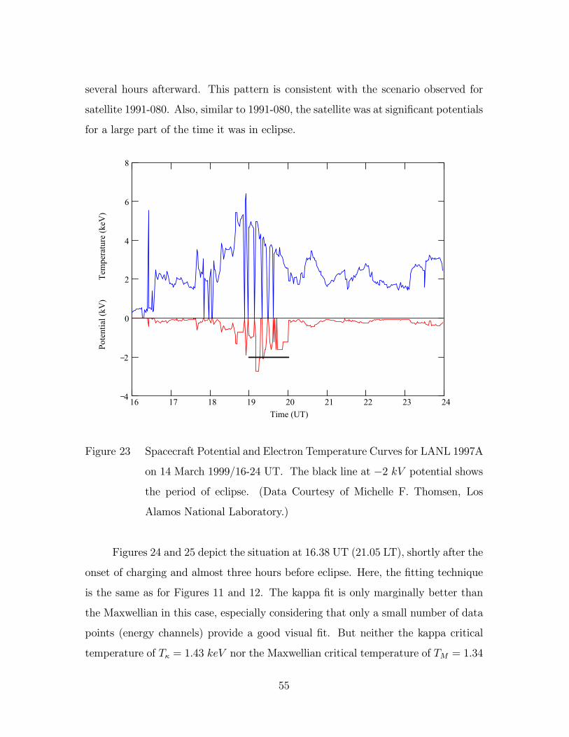
several hours afterward. This pattern is consistent with the scenario observed for

satellite 1991-080. Also, similar to 1991-080, the satellite was at significant potentials

for a large part of the time it was in eclipse.

16 17 18 19 20 21 22 23 244

2

0

2

4

6

8

Time (UT)

Pote

ntia

l (kV

)

T

empe

ratu

re (k

eV)

Figure 23 Spacecraft Potential and Electron Temperature Curves for LANL 1997A

on 14 March 1999/16-24 UT. The black line at −2 kV potential showsthe period of eclipse. (Data Courtesy of Michelle F. Thomsen, Los


Figures 24 and 25 depict the situation at 16.38 UT (21.05 LT), shortly after the

onset of charging and almost three hours before eclipse. Here, the fitting technique

is the same as for Figures 11 and 12. The kappa fit is only marginally better than

the Maxwellian in this case, especially considering that only a small number of data

points (energy channels) provide a good visual fit. But neither the kappa critical

temperature of Tκ = 1.43 keV nor the Maxwellian critical temperature of TM = 1.34

55

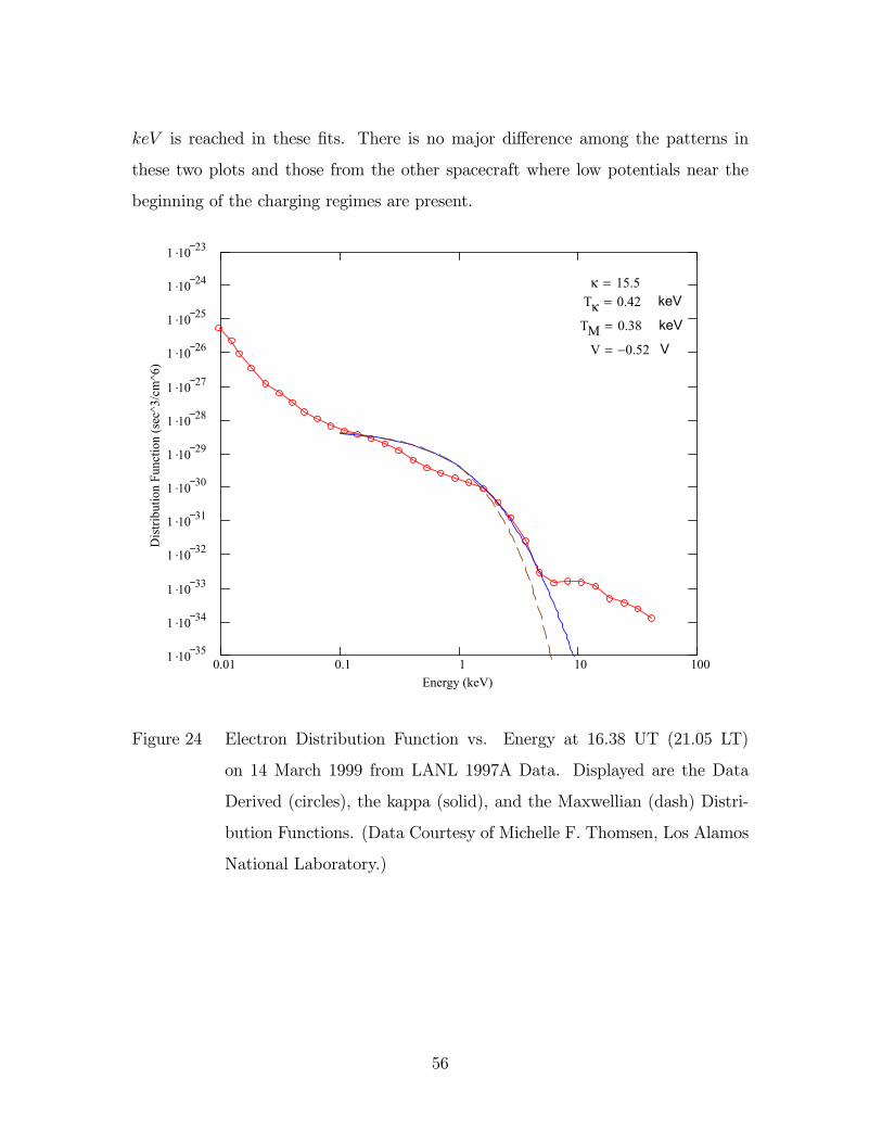
keV is reached in these fits. There is no major difference among the patterns in

these two plots and those from the other spacecraft where low potentials near the

beginning of the charging regimes are present.

0.01 0.1 1 10 1001 .10 35

1 .10 34

1 .10 33

1 .10 32

1 .10 31

1 .10 30

1 .10 29

1 .10 28

1 .10 27

1 .10 26

1 .10 25

1 .10 24

1 .10 23

Energy (keV)

Dis

tribu

tion

Func

tion

(sec

^3/c

m^6

)

κ 15.5= Tκ 0.42= keV

TM 0.38= keV

V 0.52−= V

Figure 24 Electron Distribution Function vs. Energy at 16.38 UT (21.05 LT)

on 14 March 1999 from LANL 1997A Data. Displayed are the Data




56

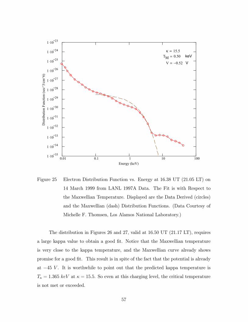
0.01 0.1 1 10 1001 .10 35

1 .10 34

1 .10 33

1 .10 32

1 .10 31

1 .10 30

1 .10 29

1 .10 28

1 .10 27

1 .10 26

1 .10 25

1 .10 24

1 .10 23

Energy (keV)

Dis

tribu

tion

Func

tion

(sec

^3/c

m^6

)

κ 15.5=TM 0.50= keV

V 0.52−= V


14 March 1999 from LANL 1997A Data. The Fit is with Respect to

the Maxwellian Temperature. Displayed are the Data Derived (circles)

and the Maxwellian (dash) Distribution Functions. (Data Courtesy of


The distribution in Figures 26 and 27, valid at 16.50 UT (21.17 LT), requires

a large kappa value to obtain a good fit. Notice that the Maxwellian temperature

is very close to the kappa temperature, and the Maxwellian curve already shows

promise for a good fit. This result is in spite of the fact that the potential is already

at −45 V . It is worthwhile to point out that the predicted kappa temperature isTκ = 1.365 keV at κ = 15.5. So even at this charging level, the critical temperature

is not met or exceeded.

57

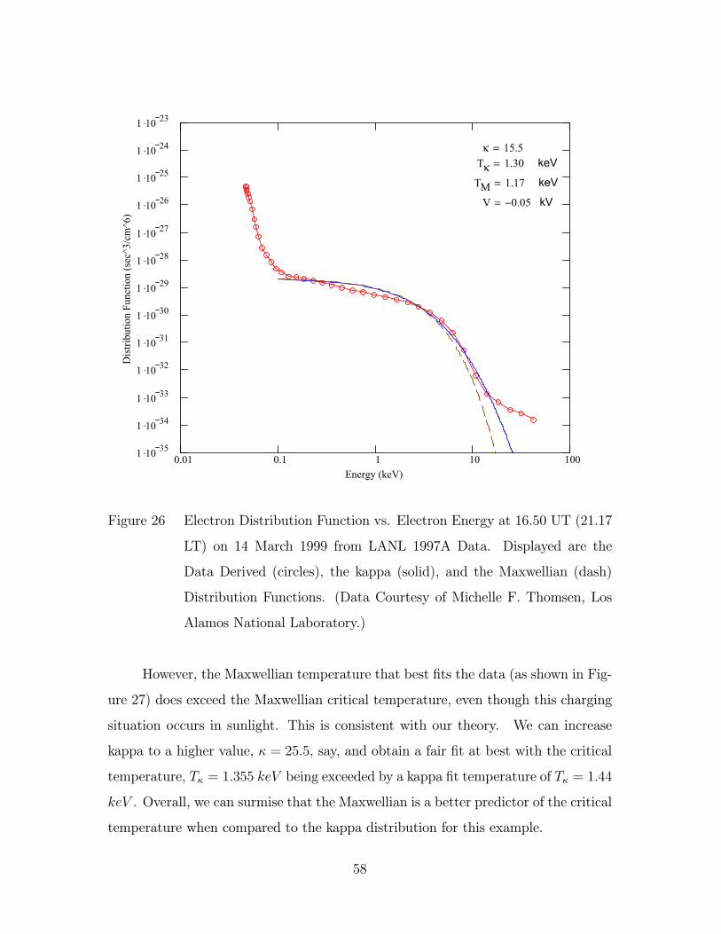
0.01 0.1 1 10 1001 .10 35

1 .10 34

1 .10 33

1 .10 32

1 .10 31

1 .10 30

1 .10 29

1 .10 28

1 .10 27

1 .10 26

1 .10 25

1 .10 24

1 .10 23

Energy (keV)

Dis

tribu

tion

Func

tion

(sec

^3/c

m^6

)

κ 15.5= Tκ 1.30= keV

TM 1.17= keV

V 0.05−= kV


LT) on 14 March 1999 from LANL 1997A Data. Displayed are the




However, the Maxwellian temperature that best fits the data (as shown in Fig-

ure 27) does exceed the Maxwellian critical temperature, even though this charging

situation occurs in sunlight. This is consistent with our theory. We can increase

kappa to a higher value, κ = 25.5, say, and obtain a fair fit at best with the critical

temperature, Tκ = 1.355 keV being exceeded by a kappa fit temperature of Tκ = 1.44

keV . Overall, we can surmise that the Maxwellian is a better predictor of the critical

temperature when compared to the kappa distribution for this example.

58

0.01 0.1 1 10 1001 .10 35

1 .10 34

1 .10 33

1 .10 32

1 .10 31

1 .10 30

1 .10 29

1 .10 28

1 .10 27

1 .10 26

1 .10 25

1 .10 24

1 .10 23

Energy (keV)

Dis

tribu

tion

Func

tion

(sec

^3/c

m^6

)

κ 15.5=TM 1.39= keV

V 0.05−= kV


LT) on 14 March 1999 from LANL 1997A Data. The Fit is with Respect

to the Maxwellian Temperature, and the Potential is −45 V . Displayedare the Data Derived (circles) and the Maxwellian (dash) Distribution

Functions. (Data Courtesy of Michelle F. Thomsen, Los Alamos Na-

tional Laboratory.)

Figure 28 shows the distribution functions at 16.98 UT (21.65 LT). At this

point, the potential has doubled as compared to the potential measured about 30

minutes before. This data plot exhibits a good kappa fit, and the critical tempera-

ture determined by the kappa value from the fit is well above the predicted critical

temperature of 1.52 keV .

59

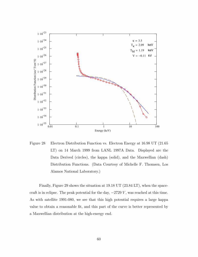
0.01 0.1 1 10 1001 .10 35

1 .10 34

1 .10 33

1 .10 32

1 .10 31

1 .10 30

1 .10 29

1 .10 28

1 .10 27

1 .10 26

1 .10 25

1 .10 24

1 .10 23

Energy (keV)

Dis

tribu

tion

Func

tion

(sec

^3/c

m^6

)

κ 3.5= Tκ 2.09= keV

TM 1.19= keV

V 0.11−= kV


LT) on 14 March 1999 from LANL 1997A Data. Displayed are the




Finally, Figure 29 shows the situation at 19.18 UT (23.84 LT), when the space-

craft is in eclipse. The peak potential for the day, −2729 V , was reached at this time.As with satellite 1991-080, we see that this high potential requires a large kappa

value to obtain a reasonable fit, and this part of the curve is better represented by

a Maxwellian distribution at the high-energy end.

60

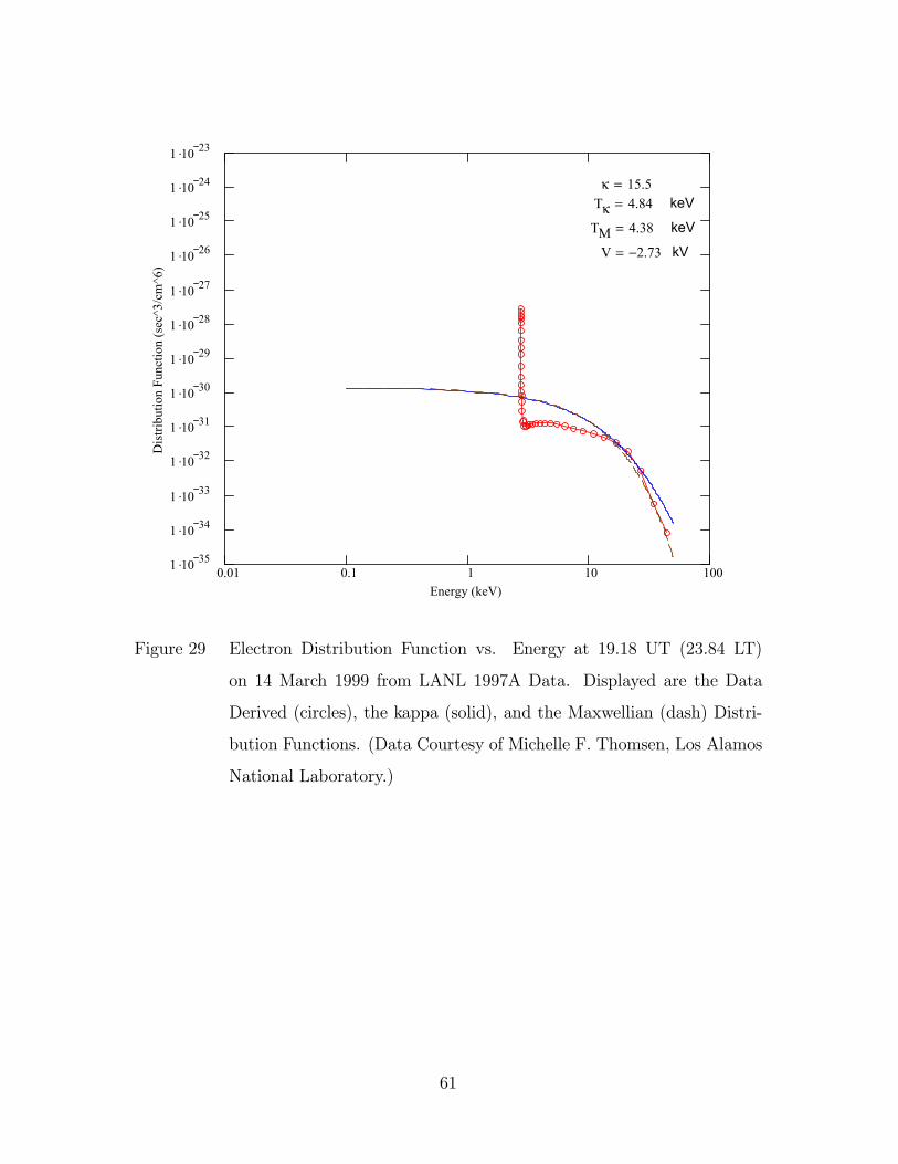
0.01 0.1 1 10 1001 .10 35

1 .10 34

1 .10 33

1 .10 32

1 .10 31

1 .10 30

1 .10 29

1 .10 28

1 .10 27

1 .10 26

1 .10 25

1 .10 24

1 .10 23

Energy (keV)

Dis

tribu

tion

Func

tion

(sec

^3/c

m^6

)

κ 15.5= Tκ 4.84= keV

TM 4.38= keV

V 2.73−= kV

Figure 29 Electron Distribution Function vs. Energy at 19.18 UT (23.84 LT)

on 14 March 1999 from LANL 1997A Data. Displayed are the Data




61

V. Results and Recommendations

5.1 Summary of Results

At charging onset in sunlight, there appears to be no non-Maxwellian, high-

energy (> 10 keV ) tail in most of the data we examined. The distributions where

charging in sunlight occurred were nearly, if not distinctly, Maxwellian in shape. So

application of the kappa distribution does not seem to contribute substantially in

such cases. Additionally, the existence of such low-level charging cases does not seem

to depend on the critical temperature charging predictions of Equation (6), which

model only incoming, backscattered, and secondary electrons. Perhaps this is due to

the fact that photoelectrons still dominate at this point. Recall that photoelectron

flux was not incorporated into the current balance equation. However, by the time

the spacecraft charges to more than about −50 V , the critical temperature criteriaare exceeded for both the kappa and the Maxwellian data fits. This is true even for

values of kappa less than 15.5, which is the threshold we used to delineate between

non-Maxwellian and Maxwellian distributions.

None of the charging cases examined contradicted critical temperature theory

— i.e., the existence of a critical temperature for significant (> 1 kV ) charging was

verified. When significant charging was observed, the kappa and the Maxwellian

critical temperature predictions, based on the solutions of the respective current

balance equations, were realized. So the critical temperature theory proved successful

in this research.

In most cases studied, very low-level (< 50 V ) charging can occur independent

of critical temperature predictions. But such cases can occur in sunlight, where

Equation (6) is not strictly valid. However, the current balance equation appeared

to be applicable when potentials greater than 50 V were observed, even in sunlight.

This held true for both the kappa and the Maxwellian forms of the equation.

62

Contrary to expectations, this research found no concrete benefit of using

the kappa distribution over the Maxwellian in low-level charging cases. Many of

the charging events commence under ambient plasma conditions that are modeled

equally well by both the Maxwellian and the kappa distributions. This was espe-

cially apparent in the LANL 1991-080 and 1997A data. The 1994-084 data seemed

to be an exception, but the reasons for this difference were not investigated in this

research.

Some of the LANL distributions that corresponded to kilovolt charging were fit

equally well by the Maxwellian distribution when compared to the kappa distribution

(see, for example, Figures 15 and 16). This result seems unphysical since the ambient

plasma is expected to be non-Maxwellian during large charging events. It may be

due to the fact that a single distribution function is inadequate to model the space

environment in such cases.

On the other hand, since the kappa distribution fits well with electron energies

above 10 keV , it may be better than the Maxwellian distribution at determining the

peak potentials that could be obtained. It has been noted that the linear dependence

of potential on temperature is only approximate (Lai and Della-Rose, 2001:927). At

higher potentials, the Maxwellian fails to determine the spacecraft charge, so the

kappa may offer promise in this regard.

5.2 Recommendations

Based on the success of the critical temperature predictions, the Air Force

Weather Agency (AFWA) should begin using these predictions for identifying GEO

charging events. At this juncture, the Maxwellian current balance equation appears

to be as successful as the kappa equation at predicting critical temperatures. Since

it is also computationally simpler than the kappa equation, it should be the equation

of choice until (if) a better tool comes along.

63

Determination of critical temperatures may require additional processing of

LANL data received by AFWA. Moreover, knowledge of the actual spacecraft ma-

terials used on monitored spacecraft would greatly aid in nailing down the critical

temperatures. Furthermore, such knowledge could help narrow down whether charg-

ing played an instrumental role in a spacecraft, or instrument, failure.

5.3 Suggestions for Further Study

Closer examination of the 14 March 1999 charging event could enhance the

understanding of the circumstances under which a given distribution function (kappa

or Maxwellian) gives the best results. Along this line, closer scrutiny might also aid

in understanding why LANL 1994-084 data fit more quickly, and definitely, to the

kappa distribution than either 1991-080 or 1997A. Recall that the data from these

latter two data sets were similar, but distinctly different from the 1994-084 data,

in that the high and low potential plots showed a tendency toward fitting with

Maxwellian distributions.

Extending the study to additional cases would help broaden the basis for com-

parison of the distribution functions. Such further examination could help to gener-

alize, or refine, conclusions made in this research.

The present research is restricted to an assumption of normal incidence. Broad-

ening the formulation of the current balance equation to include angle-dependent

secondary and backscattered coefficients would aid in analysis of “dwell time” near

the surface, allowing for more secondaries to be produced (Hastings and Garrett,

1996:150). The coefficients for isotropic incidence are made available by Lai (1991:1630-

1631).

Hellberg and Mace (2002) discuss the benefits of using a kappa-Maxwellian

distribution in plasma dispersion functions. Due to the anisotropy of space plasmas,

using the kappa distribution in a parallel temperature relation and the Maxwellian

in the perpendicular could possibly result in a more inclusive fit. The applicability of

64

this approach to current balance has not been investigated and is merely a suggestion

for consideration. However, since LANL instruments take parallel and perpendicular

electron temperature measurements, there may be some applicability.

Concurrent with increased charging, the forbidden region becomes evident,

and the high-energy tail distribution increases. This brings about an “elbow” at

the cut off point. There is currently no explanation for this, so the significance of

this feature, if any, is undetermined. The presence of this “elbow” is highlighted in

Section 4.2.

65

Appendix A. Determination of Eclipse Periods for Spacecraft in

Geosynchronous Orbit

The LANL data examined for this research provided spacecraft location in terms

of geographic coordinates (GEO). The GEO coordinate system is the same as that

used to identify locations on Earth (latitude and longitude). This system is oriented

with respect to the earth’s spin axis and equator. However, the coordinate system

reported in the LANL data is spacecraft centered (Thomspen, et al., 1999:19), so

the reported values must be divided by RE.

As per a suggestion by Michelle Thomsen of the Los Alamos National Labo-

ratory, the procedure for determining whether or not a spacecraft is in eclipse is to

convert the spacecraft location coordinates from GEO to GSM (see, for example,

Kivelson and Russell, 1995:Appendix 3) and verify if SQRT(YGSM2 + ZGSM2) < 1

(personal correspondence between M. Thomsen and D. Della-Rose, November 2002).

This appeared to work well since the times determined to be eclipse periods were

near spacecraft local midnight.

The geocentric solar magnetospheric system (GSM) is oriented with respect to

the earth-sun line and the earth’s magnetic dipole (though, not parallel to this dipole)

which is offset from the spin axis by about 11◦ latitude. The critical difference that

makes this system useful for determining eclipse is that the satellite will be opposite

the sun in the plane of the earth-sun line at equatorial latitudes near equinox and,

therefore, in the earth’s shadow. In addition to the criteria mentioned above, it

was necessary to ensure the spacecraft was not on the dayside of its orbit since

the critical criteria SQRT(YGSM2 + ZGSM2) < 1 occurred both in the noon and

midnight sectors.

The verification of the criteria SQRT(YGSM2 + ZGSM2) < 1 was accom-

plished by converting GEOPACK (Tsyganenko, 2001) library FORTRAN code into

MATLABR°(with modifications specific to the problem at hand). GEOPACK is a

66

software package designed to aid scientists in converting among various space physics

related coordinate systems for research and analysis purposes.

The output was imported into MathcadR°and graphically incorporated into

Figures 2 and 3 as well as similar figures in following sections.

67

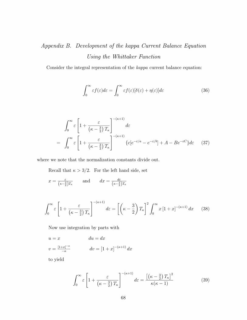
Appendix B. Development of the kappa Current Balance Equation

Using the Whittaker Function

Consider the integral representation of the kappa current balance equation:

Z ∞

0

εf(ε)dε =

Z ∞

0

εf(ε)[δ(ε) + η(ε)]dε (36)

Z ∞

0

ε

"1 +

ε¡κ− 3

2

¢Tκ

#−(κ+1)dε

=

Z ∞

0

ε

"1 +

ε¡κ− 3

2

¢Tκ

#−(κ+1){c[e−ε/a − e−ε/b] +A−Be−εC}dε (37)

where we note that the normalization constants divide out.

Recall that κ > 3/2. For the left hand side, set

x = ε

(κ−32)Tκ

and dx = dε

(κ− 32)Tκ

Z ∞

0

ε

"1 +

ε¡κ− 3

2

¢Tκ

#−(κ+1)dε =

·µκ− 3

2

¶Tκ

¸2 Z ∞

0

x [1 + x]−(κ+1) dx (38)

Now use integration by parts with

u = x du = dx

v = [1+x]−κ

−κ dv = [1 + x]−(κ+1) dx

to yield

Z ∞

0

ε

"1 +

ε¡κ− 3

2

¢Tκ

#−(κ+1)dε =

£¡κ− 3

2

¢Tκ¤2

κ(κ− 1) (39)

68

which is also the coefficient of A on the right hand side of the equation.

With α = 1/a, 1/b, or C as applicable, for the right hand side, set

c− a− 1 = −(κ+ 1) a− 1 = 1

c− a = −κ a = 2

c− 2 = −κ

c = 2− κ

u = εα z =¡κ− 3

2

¢Tκα

Substituting these values into the Whittaker function (Morse and Feshbach,

1954:612,672):

U2(a|c|z) = eiaπz−a

Γ(a)

Z ∞

0

e−uua−1h1 +

u

z

ic−a−1du (40)

and we note that a = 2 yields

ei2πz−2 = z−2

Γ(2) = 1

and apply this term by term except for A. We get

Z ∞

0

e−εαεα2−1"1 +

εα¡κ− 3

2

¢Tκα

#2−κ−2−1d (εα)

= α2Z ∞

0

e−εαε

"1 +

ε¡κ− 3

2

¢Tκ

#−(κ+1)dε (41)

=

·µκ− 3

2

¶Tκα

¸2U2(2|2− κ|

µκ− 3

2

¶Tκα) (42)

69

Therefore,

Z ∞

0

e−εαε

"1 +

ε¡κ− 3

2

¢Tκ

#−(κ+1)dε =

·µκ− 3

2

¶Tκ

¸2U2(2|2− κ|

µκ− 3

2

¶Tκα)

(43)

Finally, replace α with 1/a, 1/b, or C representing the terms on the right hand

side. Now set the left hand side equal to the right hand side and simplify to get

κ(κ− 1){c[U2(2|2− κ|µκ− 3

2

¶Tκa)− U2(2|2− κ|

µκ− 3

2

¶Tκb)]

−BU2(2|2− κ|µκ− 3

2

¶TκC)}+A− 1

= 0 (44)

The solution Tκ of this equation, for a given κ, is the critical temperature for

the onset of spacecraft charging.

70

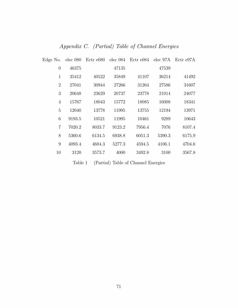
Appendix C. (Partial) Table of Channel Energies

Edge No. elec 080 Ectr e080 elec 084 Ectr e084 elec 97A Ectr e97A

0 46375 47135 47539

1 35412 40522 35849 41107 36214 41492

2 27041 30944 27266 31264 27586 31607

3 20648 23629 20737 23778 21014 24077

4 15767 18043 15772 18085 16008 18341

5 12040 13778 11995 13755 12194 13971

6 9193.5 10521 11995 10461 9289 10643

7 7020.2 8033.7 9123.2 7956.4 7076 8107.4

8 5360.6 6134.5 6938.8 6051.3 5390.3 6175.9

9 4093.4 4684.3 5277.3 4594.5 4106.1 4704.6

10 3120 3573.7 4000 3492.8 3100 3567.8

Table 1 (Partial) Table of Channel Energies

71

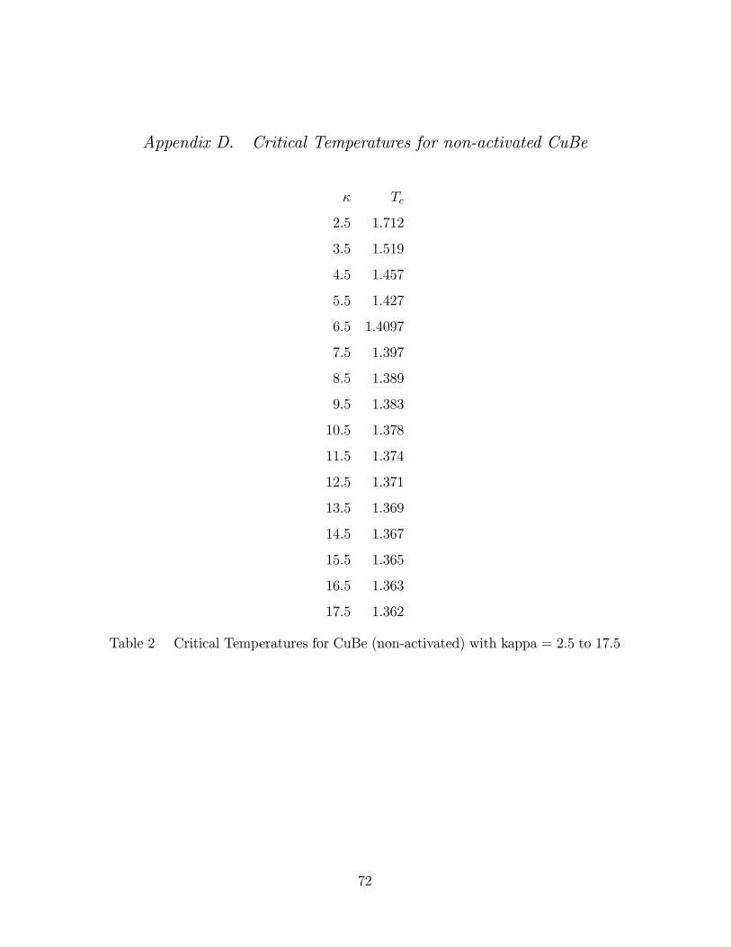
Appendix D. Critical Temperatures for non-activated CuBe

κ Tc

2.5 1.712

3.5 1.519

4.5 1.457

5.5 1.427

6.5 1.4097

7.5 1.397

8.5 1.389

9.5 1.383

10.5 1.378

11.5 1.374

12.5 1.371

13.5 1.369

14.5 1.367

15.5 1.365

16.5 1.363

17.5 1.362

Table 2 Critical Temperatures for CuBe (non-activated) with kappa = 2.5 to 17.5

72

Bibliography

Abramowitz, Milton and Irene A. Stegun, eds. Handbook of Mathematical Func-tions. Washington, DC: National Bureau of Standards, 1964.

Carpenter, D. L. “Whistler Evidence of a ‘Knee’ in the Magnetospheric IonizationDensity Profile.” Journal of Geophysical Research, 68 (No. 6):1675-1682 (March1963).

Christon, S. P. and others. “Energy Spectra of Plasma Sheet Ions and Electronsfrom 12650 eV/e to 1261 MeV During Plasma Temperature Transitions.” Journalof Geophysical Research, 93 (No. A4):2652-2572 (April 1988).

DeForest, Sherman E. “Spacecraft Charging at Synchronous Orbit.” Journal ofGeophysical Research, 19:577-616 (November 1981).

Gringauz, K. I. “The Structure of the Ionized Gas Envelope of Earth from DirectMeasurements in the USSR of Local Charged Particle Concentrations.” Planetaryand Space Science, 11:281-296 (1963).

Hastings, Daniel and Henry Garrett. Spacecraft-Environment Interactions. Cam-bridge: Cambridge University Press, 1996.

Kivelson, Margaret G. and Christopher T. Russell, eds. Introduction to SpacePhysics. Cambridge: Cambridge University Press, 1995.

Lai, Shu T. “Spacecraft Charging Thresholds in Single and Double MaxwellianSpace Environments.” IEEE Trans on Nuclear Science., 38:1629-1634 (December1991).

Lai, Shu T. “Lectures on Spacecraft Charging and Mitigation.” Graduate SchoolProgramme, Space Physics Department, Umea University, Kiruna, Sweden,September/October 1999.

Lai, Shu T. and Devin J. Della-Rose. “Spacecraft Charging at GeosynchronousAltitudes: New Evidence of the Existence of Critical Temperature.” Journal ofSpacecraft and Rockets, 38 (No. 6): 922-928 (November/December 2001).

Lai, Shu T. and M. Tautz. “Critical Temperature for the Onset of Spacecraft Charg-ing at Geosynchronous Altitudes: A Statistical Study.” EOS Trans. AGU, 83(19),Spring Meet. Suppl., Abstract SM52A-12, 2002.

Hellberg, M.A. and R.L. Mace. “Generalized Plasma Dispersion Function for aPlasma with a kappa-Maxwellian Velocity Distribution.” Physics of Plasmas, Vol.9 (No. 5):1495-1504 (May 2002).

Meyer-Vernet, Nicole: “How Does the Solar Wind Blow? A Simple Kinetic Model.”European Journal of Physics, 20: 167-176 (February 1999).

73

Meyer-Vernet, Nicole: “Large Scale Structure of Planetary Environments: TheImportance of Not Being Maxwellian.” Planetary and Space Science, 49: 247-260(May 2001).

Morse, Philip M. and Herman Feshbach.Methods of Theoretical Physics. New York:McGraw-Hill Book Company, 1953.

Parks, George K. Physics of Space Plasmas. Reading, MA:Perseus Books, 1991.

Prokopenko, S. M. L. and J. G. Laframboise. “High-Voltage Differential Chargingof Geostationary Spacecraft.” Journal of Geophysical Research, 85 (No. A8): 4125-4131 (August 1980).

Rubin, A., Garrett, H. B., and A. H. Wendel: “Spacecraft Charging on ATS-5.”Air Force Geophysics Laboratory, AFGL-TR-80-0168, AD-A090508, 1980.

Sanders, N. L. and G. T. Inouye. “Secondary Emission Effects on Spacecraft Charg-ing: Energy Distribution Considerations.” Spacecraft Charging Technology1978, Ed.R. C. Finke and C. P. Pike. 747-755, Air Force Geophysics Laboratory. NASA-2071,AD-A084626, 1978.

Sternglass, Ernest J. “Backscattering of Kilovolt Electrons from Solids.” PhysicalReview, 95 (No.2):345 (July 1954).

Su, Yi-Jiun and others. “Plasmaspheric Observations at Geosynchronous Orbit.”Journal of Atmospheric and Solar-Terrestrial Physics, 63:1185-1197 (July, 2001).

Summers, Danny and Richard M. Thorne. ”The Modified Plasma Dispersion Func-tion.” Physics of Fluids B, Vol. 3 (No. 8):1835-1847 (August 1991).

Thomsen, Michelle and others. ”Calculation of Moments from Measurements by theLos Alamos Magnetospheric Plasma Analyzer.” Los Alamos National Laboratory.LA-13566-MS, May 1999.

Tsyganenko, N. A. “GEOPACK.” FORTRAN Subroutines: SUN, RECALC,GEOGSM. http://www-spof.gsfc.nasa.gov/Modeling/geopack.html. 27 November2002.

Vasyliunas, Vytenis M. ”A Survey of Low-Energy Electrons in the Evening Sectorof the Magnetosphere with OGO 1 and OGO 3.” Journal of Geophysical Research,73 (No. 9): 2839-2884 (May 1968).

74

Vita

Capt Harris entered service in the United States Air Force in 1984. He served

as a Russian linguist before obtaining a commission through the Air Force Airman

Education and Commissioning Program in 1995. During the program, he earned a

B.S. in Meteorology and one in Mathematics at The Florida State University.

As an Air Force weather officer, he has served at Mountain Home AFB, ID

(366 OSS/OSW); Camp Red Cloud, ROK (Det 2, 607WS); and Shaw AFB, SC (28

OWS). He authored this thesis as a student at the Air Force Institute of Technology,

Wright-Patterson AFB, OH. His follow-on assignment is to Offutt AFB, NE.

75

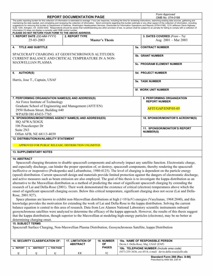
REPORT DOCUMENTATION PAGE Form Approved OMB No. 074-0188

The public reporting burden for this collection of information is estimated to average 1 hour per response, including the time for reviewing instructions, searching existing data sources, gathering and maintaining the data needed, and completing and reviewing the collection of information. Send comments regarding this burden estimate or any other aspect of the collection of information, including suggestions for reducing this burden to Department of Defense, Washington Headquarters Services, Directorate for Information Operations and Reports (0704-0188), 1215 Jefferson Davis Highway, Suite 1204, Arlington, VA 22202-4302. Respondents should be aware that notwithstanding any other provision of law, no person shall be subject to an penalty for failing to comply with a collection of information if it does not display a currently valid OMB control number. PLEASE DO NOT RETURN YOUR FORM TO THE ABOVE ADDRESS. 1. REPORT DATE (DD-MM-YYYY)

25-03-2003 2. REPORT TYPE

Master’s Thesis

3. DATES COVERED (From – To) Aug 2001 – Mar 2003

5a. CONTRACT NUMBER

5b. GRANT NUMBER

4. TITLE AND SUBTITLE SPACECRAFT CHARGING AT GEOSYNCHRONOUS ALTITUDES: CURRENT BALANCE AND CRITICAL TEMPERATURE IN A NON-MAXWELLIAN PLASMA

5c. PROGRAM ELEMENT NUMBER

5d. PROJECT NUMBER 5e. TASK NUMBER

6. AUTHOR(S) Harris, Jose T., Captain, USAF 5f. WORK UNIT NUMBER

7. PERFORMING ORGANIZATION NAMES(S) AND ADDRESS(S) Air Force Institute of Technology Graduate School of Engineering and Management (AFIT/EN) 2950 Hobson Street, Building 640 WPAFB OH 45433-7765

8. PERFORMING ORGANIZATION REPORT NUMBER AFIT/GAP/ENP/03-05

10. SPONSOR/MONITOR’S ACRONYM(S)

9. SPONSORING/MONITORING AGENCY NAME(S) AND ADDRESS(ES) HQ AFWA/XOGX 106 Peacekeeper Dr Suite 2N3 Offutt AFB, NE 68113-4039

11. SPONSOR/MONITOR’S REPORT NUMBER(S)

12. DISTRIBUTION/AVAILABILITY STATEMENT APPROVED FOR PUBLIC RELEASE; DISTRIBUTION UNLIMITED.

13. SUPPLEMENTARY NOTES 14. ABSTRACT Spacecraft charging threatens to disable spacecraft components and adversely impact any satellite function. Electrostatic charge, and especially discharge, can hinder the proper operation of, or destroy, spacecraft components, thereby rendering the spacecraft ineffective or inoperative (Prokopenko and Laframboise, 1980:4125). The level of charging is dependent on the particle energy (speed) distribution. Current spacecraft design and materials provide limited protection against the dangers of electrostatic discharge, and active measures such as beam emission are also employed. The goal of this thesis is to investigate the kappa distribution as an alternative to the Maxwellian distribution as a method of predicting the onset of significant spacecraft charging by extending the research of Lai and Della-Rose (2001). Their work demonstrated the existence of critical (electron) temperatures above which the onset of significant spacecraft charging occurs. Below this critical temperature, significant charging does not occur (Lai and Della-Rose, 2001:927). Space plasmas are known to exhibit non-Maxwellian distributions at high (>10 keV) energies (Vasyliunas, 1968:2840), and this knowledge provides the motivation for extending the work of Lai and Della-Rose to the kappa distribution. Solving the current balance equation is central to this area of research. Data from Los Alamos National Laboratory scientific instruments onboard geosynchronous satellites were analyzed to determine the efficacy of the kappa approach. However, the results of this thesis suggest that the kappa distribution, though superior to the Maxwellian at modeling high-energy particles (electrons), may be no better at determining charging onset. 15. SUBJECT TERMS Spacecraft Surface Charging, Non-Maxwellian Plasma Distribution, Geosynchronous Satellite, kappa Distribution

16. SECURITY CLASSIFICATION OF: 19a. NAME OF RESPONSIBLE PERSON Devin J. Della-Rose, Maj, USAF (ENP)

a. REPORT

U

b. ABSTRACT

U

c. THIS PAGE

U

17. LIMITATION OF ABSTRACT

UU

18. NUMBER OF PAGES

92

19b. TELEPHONE NUMBER (Include area code) (937) 255-3636, ext 4514; e-mail: [email protected]

Standard Form 298 (Rev. 8-98) Prescribed by ANSI Std. Z39-18

Documents

Spacecraft Charging at Geosynchronous Altitudes: Current