Sources of Geographic Variation in Health Care

Sources of Geographic Variation in Health Care:Evidence from Patient Migration

Online Appendix

Amy FinkelsteinMIT and NBER

Matthew GentzkowStanford and NBER

Heidi WilliamsMIT and NBER

April 2016

1 Corrected Health Measures

Evidence in Song et al. (2010) suggests that standard health measures based on diagnoses recorded in claims datainclude an important place-specific measurement error. A given HRR’s estimated rate of hypertension, for example, isbased on the number of patients who have had recent Medicare claims that included a code for hypertension diagnosis.Such codes are typically only recorded when a patient visits a doctor and receives a billable treatment related to herhypertension.1 A high-utilization and a low-utilization HRR that had the same underlying rates of hypertension willtherefore tend to have very different recorded rates: patients in the high-utilization area may visit the doctor moreoften, and be more likely to receive billable treatment for their hypertension conditional on visiting. Song et al.(2010) use an empirical strategy similar to ours to show that patients who move across quintiles of the HRR spendingdistribution experience large, discrete changes in health status as measured by standard proxies, consistent with ahigher probability of diagnoses being recorded in claims in more intensive areas.

To correct for this measurement error, we assume that measured health hmeasi jt is a function of true, patient health

hit and a measurement error whose distribution depends on place and year:

hmeasi jt = hit +ξi jt ,(1)

where

hit = αhi + xitβ

h(2)ξi jt = γ

hj + τ

ht + ε

hi jt .(3)

Note that Online Appendix equation (1) has the same form as equation (2) of the main text. We use the same strategybased on patient movers to identify the patient component of health (hit) separately from the place and year-specificmeasurement error (ξi jt ), and assume that the analogous identifying conditions hold. Note that we interpret the differ-ential trends for movers captured by the relative-year fixed effects and age dummies in xit as changes in true health.2

We consider the four standard health status measures discussed in Section V and defined in more detail in OnlineAppendix Section 3.2. For HCC score, we define hmeas

i jt to be the log of HCC score; for all the other measures, wedefine hmeas

i jt to be each measure plus one, following our strategy when we analyzed utilization. We estimate equation(1) by OLS, and form estimates hit of true health for each patient-year.

1See chapter 23 of the Medicare Claims Processing Manual (Centers for Medicare and Medicaid Services 2014).2These components may in fact represent a mix of true health and measurement error. For example, older patients may both have more chronic

conditions and be more likely to have a given chronic condition recorded in claims. We include these terms in hit for simplicity; this should beborne in mind in interpreting the results.

1

Online Appendix Figure 1 shows an event study analogous to Figure VI of the main text using the number ofchronic conditions as the outcome. Consistent with Song et al. (2010), we see sharp changes in measured health statuswhen patients move. There is no meaningful pre-trend and a small post-trend. The size of the jump is roughly 0.5,implying that half of the cross-area differences in measured health are due to measurement error.3

The event-study figures also shed light on the nature of the measurement process. For example, Online AppendixFigure 1 shows that measured health adjusts immediately on move with little post-move adjustment, and OnlineAppendix Figure 15 shows that the adjustment is symmetric for moves up and moves down. This pattern may suggestthat the endogenous component is mainly related to the recording of diagnoses in claims rather than to diagnoses per se.If the primary force were endogeneity of diagnoses (that is, patients in some places learn they have hypertension whilethe hypertension elsewhere goes undiagnosed), we would have expected to see more adjustment up than adjustmentdown.

2 Definition of Utilization Measures

2.1 Overall Utilization

Following standard practice in the literature, we construct our health care utilization measure by aggregating careprovided to Medicare beneficiaries as recorded in the inpatient, outpatient, and carrier claims data. The inpatient filerecords payments to inpatient hospital providers (such as hospitals), the outpatient file records payments to institutionaloutpatient providers (such as hospital outpatient departments), and the carrier file records payments to physicians andother non-institutional providers (such as independent ambulance providers). Following the methodology of Gottliebet al. (2010),4 we transform the claims (spending) data in these files into a quantity-based measure of utilization thatis stripped of geographic variation in Medicare prices. This section describes our approach. The price adjustmentprocedures of Gottlieb et al. (2010) are specific to the types of claims examined, so we separately describe our priceadjustment procedure for inpatient, outpatient, and carrier claims. Our measure of health care utilization excludesseveral dimensions of care, including durable medical equipment, home health agency care, hospice care, skillednursing facility care, inpatient rehabilitation facility care, and claims filed through Medicare Part D (prescription drugcoverage). Recent work (Newhouse and Garber 2013) has suggested there is substantial variation in these additionalmeasures of care.

2.1.1 Inpatient Claims

Inpatient payments are determined by an algorithm that we now describe.5 First, Medicare sets so-called “standardizedpayment amounts” per discharge. These base payment amounts are meant to capture “the operating and capital coststhat efficient facilities would be expected to incur in furnishing covered inpatient services.” For example, for the fiscalyear 2010, the operating base rate was $5,223, and the capital rate was $430.

Second, this base payment is adjusted by an area wage index to “reflect the expected differences in local marketprices for labor.” The wage index is revised annually. The wage index is applied to the labor-related portion of thebase payment, where the labor-related portion is defined differently across hospitals as a function of the wage index:for hospitals with a wage index above 1.0, CMS applies a labor share of 68.8 percent; for hospitals with a wage indexless than or equal to 1.0, CMS applies a labor share of 62 percent.

Third, the wage-adjusted base payment is adjusted for case mix using diagnosis related group (DRG) relativeweights. To understand these weights, note that over the time period of our data, inpatient payments are covered bya prospective payment system. Inpatient claims are centered around DRGs for specific services. Each DRG has arelative weight that aims to reflect “the expected relative costliness of inpatient treatment for patients in that group.”DRG weights are set annually.

3Online Appendix Figure 15 presents event-study figures for our other health measures. Online Appendix Table 10 presents decompositions ofthe variation in health status analogous to Table II that confirm the share due to place-specific measurement error is about 0.5 to 0.6.

4See http://www.dartmouthatlas.org/downloads/papers/std_prc_tech_report.pdf.5This section is based on details from various MedPAC reports describing reimbursement rules for inpatient services.

2

http://www.dartmouthatlas.org/downloads/papers/std_prc_tech_report.pdf

Finally, several factors are added to this wage- and case-adjusted base payment, including an adjustment for fa-cilities that operate a resident training program (indirect medical education payment, IME), an adjustment for facil-ities that treat a disproportionate share of low-income patients (DSP), adjustments for bad debts (non-payments ofdeductibles and copayments by beneficiaries), new technology payments, and outlier payments for particularly ex-pensive cases. Payments are reduced in cases of transfers, and critical access hospitals are paid separately on a costbasis.

Taken together, this description suggests that the key geographic price variation that we want to strip out comesfrom the area wage index, IME payments to residency programs, DSP payments to disproportionate share hospitals,bad debt adjustments, new technology payments, and outlier payments. In practice, our data do not include IMEpayments to residency programs, DSP payments to disproportionate share hospitals, bad debt adjustments, or newtechnology payments, so only the area wage index and outlier payments are relevant. Following Gottlieb et al. (2010),we define the price-adjusted inpatient level utilization for individual i’s receipt of procedure k in region j at time t tobe:

Uik jt = Pt ×DRGkt +OPikt/WI jt

where Pt is the national-level base payment rate at time t (not wage-adjusted), DRGik jt is the DRG weight used todetermine payment for procedure k, OPikt is the outlier payment (if any), and WI jt is the wage index factor defined as

WI jt = 0.25+0.75× (wage index for region j at time t) .

Gottlieb et al. (2010) clarify that they wage-adjust the outlier payments to account for differences in price level costsacross regions, where region is defined as the provider’s Core-Based Statistical Area (CBSA). If a provider is notlocated in a CBSA, we use the state’s rural wage index. For the few cases in which a provider’s CBSA was uncertainand it was located within a state that does not have a rural wage index (MA, NJ, RI, DC, PR), we used the median ofall the urban wage indices in that state for that year.

To ensure that price-adjusted hospital expenditures add up to aggregated actual expenditures, we follow Gottliebet al. (2010) and make a further adjustment (λ ) to ensure the adding up constraint, where λ is defined implicitly by:

∑∑∑∑ ik jtTotal Hospital Expenditures = λ ∑∑∑∑ ik jtUik jt

where the sum is taken over all age groups (including the under 65 population) after randomly dropping 75 percent ofthe non-movers. Note that Gottlieb et al. (2010) further adjust for age, sex, and race, which we do not do.

2.1.2 Carrier Claims

Carrier claim based reimbursements are centered around Healthcare Common Procedure Coding System (HCPCS)codes for specific services.6 Payments at the HCPCS code level—with the caveat that HCPCS codes are sometimesmore specific when “modifier” codes are included—are determined as follows.7

First, CMS estimates the “amount of work required to provide a service, expenses related to maintaining a practice,and liability costs.” Each of these three components—work (W), practice expense (PE), and professional liabilityinsurance (PLI)—are assigned a relative value unit (RVU) weight.

Second, each of the three RVU components (W, PE, PLI) are adjusted by separate geographic practice cost indices(GPCIs).

Third, the GPCI-weighted sum of the three RVU components is then multiplied by a conversion factor of 0.8,reflecting that beneficiaries pay 20 percent of carrier costs directly through their coinsurance.

Finally, several payment modifiers are applied, including adjustments for different types of providers (physiciansversus non-physicians, participating versus nonparticipating physicians), geographic bonuses paid to providers in des-ignated “health provider shortage areas” (HPSAs), and service-specific adjustments for primary care and major surgi-cal procedures.

6This section is based on details from various MedPAC reports describing reimbursement rules for carrier claims.7We follow Gottlieb et al.’s (2010) treatment of claims associated with multiple modifier codes, and use only the first modifier code.

3

Taken together, this description suggests that the key geographic price variation that we want to strip out comesfrom the three RVU-specific geographic practice cost indices (GPCIs) and the geographic specific HPSA bonuses. Got-tlieb et al. (2010) estimate carrier-specific utilization by—for each HCPCS code (and HCPCS-modifier code combi-nation, if applicable)—merging on national (that is, not area-specific) RVU weight as documented in a CMS-providedfee schedule. Some HCPCS codes have an RVU of zero in the fee schedule (mainly due to statutory exclusions) or donot merge to the fee schedule. For such codes, we follow Gottlieb et al. (2010) and assign the RVU weight to be themedian carrier payment by HCPCS code-modifier-year, divided by a year-specific price conversion factor.

As with our inpatient claims calculation, we make an adjustment to ensure that price-adjusted hospital expendituresadd up to aggregated actual expenditures. Gottlieb et al. (2010) use a different standard price adjustment for ambulatorysurgery centers, anesthesia, and certified nurse anesthetists which we do not do for simplicity.

2.1.3 Outpatient Claims

Like inpatient services, outpatient payments are covered by a prospective payment system over the time period of ourdata.8 Outpatient claims are centered around ambulatory payment classifications (APCs) for specific services. EachAPC has a relative weight that aims to reflect “resource requirements of services.” APC weights are set annually, andpayments are determined as follows.

First, APC weights are multiplied by a wage-adjusted conversion factor. Specifically, the labor share—set at 60percent for all institutions—is adjusted by a hospital wage index, while the remaining (40 percent) non-labor share isunadjusted.9 Second, adjustments are made for cancer hospitals, children’s hospitals, rural hospitals with 100 or fewerbeds, and sole community hospitals. Finally, outlier payments can be made for particularly expensive cases.

Taken together, this description suggests that the key geographic price variation that we want to strip out comesfrom the wage index and the hospital type adjustments. Gottlieb et al. (2010) simplify this to focus on the wage index.Specifically, they construct

WI jt = 0.4+0.6× (wage index for region j at time t)

and divide payments to providers by this wage adjustment factor. As with inpatient and carrier claims, we also makean adjustment to ensure that price-adjusted outpatient expenditures add up to aggregated actual expenditures.

2.2 Components of Overall Utilization

To explore our aggregate utilization estimates in more detail, we construct a number of disaggregated measures. Thefirst four measures (inpatient, outpatient, emergency room, and other) are mutually exclusive and exhaustive.

• Inpatient utilization. This measures utilization recorded in the inpatient claims data excluding claims with rev-enue center codes for emergency room services. We construct a quantity-based measure of inpatient utilizationthat is stripped of geographic variation in Medicare prices (as described above), as well as an indicator for anyhospitalization (defined as any inpatient utilization).

• Outpatient utilization. This measures utilization recorded in the outpatient claims data, including office visitsrecorded in the carrier claims data, excluding claims with revenue center codes for emergency room services. Weconstruct a quantity-based measure of outpatient utilization that is stripped of geographic variation in Medicareprices (as described above).

8This section is based on a 2010 MedPAC report summarizing the reimbursement rule for outpatient claims. Seehttp://www.medpac.gov/documents/medpac_payment_basics_10_opd.pdf.

9New technology APCs are reimbursed differently, but as best we can tell are not addressed by Gottlieb et al. (2010).

4

http://www.medpac.gov/documents/medpac_payment_basics_10_opd.pdf

• Emergency room utilization. This measures utilization recorded in inpatient or outpatient claims with revenuecenter codes for emergency room services, together with carrier claims that take place in an emergency room.We construct a quantity-based measure of emergency room utilization that is stripped of geographic variation inMedicare prices (as described above), in addition to an indicator for any emergency room utilization.

• Other utilization. This includes carrier claims not included in our inpatient, outpatient, and emergency roomutilization measures described above; this includes laboratory claims, ambulance claims, nursing facility claims,and skilled nursing facility claims.

• Whether a patient has seen a primary care physician or (separately) a specialist physician. Our definitionof primary care physicians and specialists follows the Dartmouth Atlas.10 Specifically, we crosswalk the primarycare and specialist definitions in the Dartmouth Atlas to the list of physician categories included in the providerspecialty table provided by the Centers for Medicare and Medicaid Services (CMS) in order to replicate thecategories listed in the Dartmouth Atlas.11 When we examine physicians in the inpatient claims data, we relyon the attending physician ID; when we examine physicians in the carrier claims data, we rely on the referringphysician ID; when we examine physicians in the outpatient claims data, we rely on the attending physician ID.

• Diagnostic and imaging tests. Our definition of diagnostic and imaging tests follows Song et al. (2010), and isbased on BETOS codes: codes beginning with T are diagnostic tests, and codes beginning with I are imagingtests.

• Preventive care procedures. We measure a count of “preventive care” procedures following those measured inthe Dartmouth Atlas and the Centers for Medicare and Medicaid:

– Mammogram is defined following the Dartmouth Atlas.12 Specifically, we define this based on CPT codes76090-76092 and 76083; ICD-9 codes 87.36 and 87.37; V codes 76.11 and 76.12; and revenue center code0403.

– Hemoglobin A1c testing, blood lipids testing, negative retinal exam, and negative retinal or dilated eyeexam are defined following the Dartmouth Atlas.13

– Ambulatory visits are defined following the Dartmouth Atlas.14

– Cardiovascular screening blood testing, seasonal influenza virus vaccine, diabetes self-management train-ing, bone mass measurements, colorectal cancer screening, pap smears, pelvic examinations, and prostatecancer screening are defined following CMS’s preventive care definitions.15 Note that for colorectal cancerscreening, we only use CPT code 82270 and HCPCS code G0328.

• Number of different doctors seen. We identify unique physicians by linking time-varying physician identifiers.The count of “different doctors seen” is constructed by summing the number of unique physicians that billed fora given patient in that year.16

Online Appendix Table 11 reports the share of patient-years for which an utilization component or health measurehas a value of zero.

10See http://www.dartmouthatlas.org/downloads/methods/research_methods.pdf, page 6.11The provider specialty table used is available at http://www.resdac.org/sites/resdac.org/files/HCFA%20Provider%20Specialty%20Table.txt.

Crosswalking from the Dartmouth Atlas definitions to the CMS-provided table is straightforward as the two sources enable an exact match.12See http://www.dartmouthatlas.org/data/table.aspx?ind=169.13See http://www.dartmouthatlas.org/data/map.aspx?ind=160.14See http://www.dartmouthatlas.org/data/table.aspx?ind=170.15See http://www.cms.gov/Medicare/Prevention/PrevntionGenInfo/Downloads/MPS_QuickReferenceChart_1.pdf.16Any provider with a unique set of identifiers is considered a different “doctor”, though these identifiers can be used for billing groups and

non-physician practitioners as well.

5

http://www.dartmouthatlas.org/downloads/methods/research_methods.pdf

http://www.resdac.org/sites/resdac.org/files/HCFA%20Provider%20Specialty%20Table.txt

http://www.dartmouthatlas.org/data/table.aspx?ind=169

http://www.dartmouthatlas.org/data/map.aspx?ind=160

http://www.dartmouthatlas.org/data/table.aspx?ind=170

http://www.cms.gov/Medicare/Prevention/PrevntionGenInfo/Downloads/MPS_QuickReferenceChart_1.pdf

3 Additional Results

3.1 Descriptive Evidence on Movers

We present additional descriptive evidence on movers and their moves. Online Appendix Figure 2 plots the distri-bution of the distance from a mover’s origin to their destination HRR. Online Appendix Figure 3 shows the distributionof movers across destination HRRs. Online Appendix Table 1 shows the distribution of movers by census division.

Online Appendix Figure 4 plots mean log utilization in each relative year for movers. Since log utilization willnaturally trend upward due to aging and the passage of time, we also plot the mean log utilization of a matched sampleof non-movers for comparison. We construct both a matched sample of non-movers from the movers’ origin HRRs, asin Figure IV, and an analogous matched sample of non-movers from the movers’ destination HRRs. The figure showsthat moving is associated with an increase in utilization in general, and with an upward spike in utilization in the yearof the move.

Table I provides some comparison of the characteristics of movers and non-movers. For additional information, wealso report results from the Health and Retirement Study (HRS). The HRS is a nationally representative longitudinalsurvey of Americans over the age of 50.17 Since 1992, the HRS has been administered in (approximately) two-yearcycles, following individuals and their spouses from their time of entry to the survey sample until their death. We usedata through 2008. Data without individual identifiers and zip code-level geographic information can be downloadedfrom the HRS website.18 Our analysis uses the restricted-access HRS data, which contains zip code-level geographicinformation, in order to identify movers. We define movers as individuals who move between HRRs. In order to defineHRRs, we merge the HRS data with a zip code-HRR crosswalk downloaded from the Dartmouth Atlas website.

Our analysis uses a version of the HRS data prepared by the RAND Corporation (RAND HRS). The RAND HRScontains most measures that are surveyed in the HRS, and aims to create variables consistent across the waves of thesurvey. We merged in the “reasons for move” question, which is not included in the RAND HRS. Waves are definedas follows: Wave 1 (1992), Wave 2 (1993 and 1994), Wave 3 (1995 and 1996), Wave 4 (1998), Wave 5 (2000), Wave6 (2002), Wave 7 (2004), Wave 8 (2006), and Wave 9 (2008).

We limit the sample to individuals aged over 65 to match our Medicare data, and define a mover as an individualwho moves between HRRs exactly once. This gives us a sample of about 22,000 individuals, observed on average forabout 4 waves (i.e., 8 years); about 10 percent of the sample moved during this time. In addition, about 1,100 of the2,000 movers answered a question about why they moved.

Online Appendix Table 2 reports summary statistics for movers and non-movers in the HRS data. It indicates thatmovers are more likely to be white, not married, and higher educated than non-movers.

Online Appendix Figure 5 shows the most common reasons given for moving.We also used the HRS to investigate time-varying correlates of moving. Specifically we estimated the following

panel-wave level regression:

MOVEit = αi + τt +δX it + εit .(4)

The dependent variable MOVEit is an indicator variable if person i is living in a different HRR in wave t than in wavet − 1. Conditional on individual fixed effects (αi) and wave fixed effects (τt ), we analyze the bivariate associationbetween various time varying covariates (X it) and the probability of moving. Online Appendix Table 3 shows theresults for different indicator variables X it . In row (1) we consider an indicator variable for whether the individual isnot married; in row (2), for whether they are separated or divorced; in row (3) for whether they are widowed; in row(4) for whether they are retired or partly retired; and in row (5) for self-reported health being “fair” or “poor” (insteadof “good”, “very good” or “excellent”).

3.2 Correlates of patient and place characteristics

We construct measures of area-level patient and place characteristics from several sources.We briefly describe themeasures and their sources here. Since we use these measures to look at the correlates of place effects and average

17The HRS (Health and Retirement Study) is sponsored by the National Institute on Aging (grant number NIA U01AG009740) and is conductedby the University of Michigan.

18See http://hrsonline.isr.umich.edu/.

6

http://hrsonline.isr.umich.edu/

patient effects in an HRR, we construct each variable at the HRR level. Online Appendix Table 12 shows the meanand standard deviation across HRRs (with each HRR weighted equally). We limit our analysis to 96 out of the 306HRRs for which we can measure all 12 of the patient and physician preference measures described below. These 96HRRs include about 60 percent of our patient sample. We now describe the data sources and variable construction foreach of our measures:

Medicare data: age, race, sex, and health measures

From our baseline sample, we construct HRR-level summary measures of basic patient demographic characteris-tics: average age, percent black, and percent female.

We also construct HRR-level averages of four standard patient health measures in our baseline sample. Thesepatient health measures are in turn constructed based on the health recorded in the diagnosis codes in the Medicareclaims data: Hierarchical Condition Categories (HCC) score, number of chronic conditions, Charlson ComorbidityIndex, and number of Iezzoni Chronic Conditions. All of these measures take diagnosis codes as inputs. They differin which diagnoses they use (although there is considerable overlap), the weights assigned to them, and the look-backperiod. The HCC score is defined by the Centers for Medicare and Medicaid Services (CMS) for use in computingMedicare payments, and is designed to approximate predicted spending given demographics (including age, gender,and Medicaid eligibility) and diagnoses coded in the previous year.19 The number of chronic conditions is a count of27 conditions defined by CMS; they are measured based on diagnoses coded in the past 1-3 years depending on thecondition.20 The Charlson Comorbidity Index (Charlson et al. 1987) is a weighted count of specific diagnoses codedin that year that is designed to predict ten-year mortality.21 The number of Iezzoni Chronic Conditions (Iezzoni et al.1994) counts diagnoses for a specific set of conditions recorded in that year.22

In the paper, we analyze adjusted measures of the log of the Hierarchical Condition Categories (HCC) score, andthe log of one plus: the count of a patient’s chronic conditions, the Charlson Comorbidity Index, and the count ofa patient’s Iezzoni Chronic Conditions. The adjustment, which is discussed more in the paper (see Section V andespecially in Online Appendix Section 1), is made to purge these measures of the place-specific measurement errorcomponent and to thus create what we refer to as our “corrected” health measures.

Census data

We turn to the Census data to construct HRR-level statistics for two additional demographic measures: incomeand education. These are based on population-wide estimates. Specifically, we average data from the 2000 census andthe five-year estimates from the 2007-2011 American Community Surveys (ACS).23 These data report (at the zip codelevel) median household income and the percent of the 25 and over population with a high school degree. To constructthe income measure, we compute the median household income across zipcodes, separately using the 2000 census dataand the 2007-2011 ACS five-year estimates; we then take the average of the two. To construct the education measure,we compute the total number of people who completed high school across all zipcodes in an HRR as a share of HRRpopulation, separately using the census data and the ACS data; we then take the average of the two.

Patient and physician preferences

We draw on two surveys conducted by Cutler et al. (2015) to create proxies for patient preferences for health care19Our HCC score derivation is based on Pope et al. (2004).20See https://www.ccwdata.org/web/guest/condition-categories. The conditions are Acquired Hypothyroidism (reference time period: 1 year),

Acute Myocardial Infarction (1 year), Alzheimer’s Disease and Related Disorders or Senile Dementia (3 years), Alzheimer’s Disease (3 years),Anemia (1 year), Asthma (1 year), Atrial Fibrillation (1 year), Benign Prostatic Hyperplasia (1 year), Breast Cancer (1 year), Cataract (1 year),Chronic Kidney Disease (2 years), Chronic Obstructive Pulmonary Disease (1 year), Colorectal Cancer (1 year), Depression (1 year), Diabetes (2years), Endometrial Cancer (1 year), Glaucoma (1 year), Heart Failure (2 years), Hip/Pelvic Fracture (1 year), Hyperlipidemia (1 year), Hyper-tension (1 year), Ischemic Heart Disease (2 years), Lung Cancer (1 year), Osteoporosis (1 year), Prostate Cancer (1 year), Rheumatoid Arthritis /Osteoarthritis (2 years), and Stroke / Transient Ischemic Attack (1 year).

21The conditions are Acute Myocardial Infarction, AIDS/HIV, Cancer, Cerebrovascular Disease, Chronic Pulmonary Disease, Congestive HeartFailure, Dementia, Diabetes with chronic complications, Diabetes without complications, Hemiplegia or Paraplegia, Metastatic Carcinoma, MildLiver Disease, Moderate or Severe Liver Disease, Peptic Ulcer Disease, Peripheral Vascular Disease, Renal Disease, and Rheumatologic Disease(Connective Tissue Disease).

22The conditions are Chronic Pulmonary Disease, Congestive Heart Failure, Coronary Artery Disease, Dementia, Diabetes With End OrganDamage, Malignant Cancer, Leukemia, Peripheral Vascular Disease, Renal Failure, and Severe Chronic Liver Disease.

23These data can be downloaded at http://factfinder.census.gov/faces/nav/jsf/pages/index.xhtml

7

https://www.ccwdata.org/web/guest/condition-categories

http://factfinder.census.gov/faces/nav/jsf/pages/index.xhtml

(ηi) and physician beliefs regarding appropriate treatment (λ j). For both measures, we average the individual-leveldata to create HRR-level summary measures. We are extremely grateful to these authors both for conducting thesesurveys and for generously sharing the data with us.

To measure patient preferences (ηi), we use Medicare beneficiaries’ survey responses to desired care in hypothet-ical cases. We use survey responses from 1,519 Medicare beneficiaries; on average we have about 16 responses perHRR. Following Cutler et al. (2015), we construct four measures of patient preferences: the share of patients in eacharea who report that they would (1) “have unneeded tests”, (2) “see unneeded cardiologist”, (3) like aggressive end-of-life care (“aggressive patient preferences ratio”), and (4) like palliative end-of-life care even if it shortens their life(“comfort patient preferences ratio”). On average in an HRR, patients report a high frequency of wanting unneededtests or seeing an unneeded cardiologist; about half report that they would like palliative end-of-life care even if itshortens life, and very few report that they would like aggressive end-of-life care.

To measure physician beliefs about appropriate treatment (λ j), we use survey responses of primary care providers(PCPs) and cardiologists (separately) to (specialty-specific) hypothetical clinical vignettes. We use survey responsesfrom 674 PCPs and 447 cardiologists. The average HRR includes responses from seven PCPs and five cardiologists;all have at least two PCPs or cardiologists. Following the classification of Cutler et al. (2015), we code each physicianas “high follow-up” or “low follow-up” if they recommend follow-up visits more (or less) frequently than clinicalguidelines would suggest; because the guidelines for the vignettes are themselves quite broad in the range of timerecommended for a follow-up visit, there is a fairly large share of physicians who are coded as neither high nor lowfollow-up. We also follow the authors’ classification and code physicians as “cowboys” if they recommend care moreintensive than the guidelines, and as “comforters” if they recommend palliative care for severely ill patients; theseare not mutually exclusive. On average in an HRR, about half of PCPs and about 30 percent of cardiologists are“comforters”; about a quarter of each are “cowboys”.

Hospital Compare Score (“Timely and Effective Care”)

We measure the average quality of hospitals in an HRR using “process of care” measures that are publicly reportedby CMS.24 These measures (also known as “timely and effective care measures”) show the share of patients with acertain condition who received certain evidence based interventions. Hospitals report their utilization of these pro-cesses to CMS, which publishes the information online and uses it to adjust hospital payments. The data pertain to alleligible patients irrespective of their insurer, and are not limited to patients covered by Medicare. The data are avail-able beginning in 2005. During years that overlap with our baseline sample (2005-2008), which we use to constructthe HRR level measures, it includes measures for the following conditions: heart attacks, heart failure, pneumonia,and (beginning in 2008) children’s asthma. The measures include, for example, the share of patients given aspirin atarrival (for heart attack patients) and the share of patients given oxygenation assessment (for pneumonia patients).25

We construct averages across measures and hospitals within an HRR for each reporting cycle, then average acrossreporting cycles within each year, and finally average across years to obtain the HRR-level measures. On average inan HRR, hospitals deliver about 80 percent of the recommended “timely and effective care.”

Physician prevalence

We construct HRR-level measures of specialists per thousand residents and PCPs per thousand residents usingcounts of physicians from the 2011 AMA Physician Masterfile, and population estimates from averaging over the2000 Census and the 2007-2011 ACS.

Hospital characteristics

We construct HRR-level measures of hospital beds per thousand residents using counts of hospital beds fromthe 1998-2008 American Hospital Association’s (AHA’s) annual survey of hospitals, and the population estimatesdescribed above. We also use the AHA data to compute the percent of hospitals in an HRR that are non-profit (asopposed to public or for-profit).

24These data can be downloaded at https://data.medicare.gov/data/archives/hospital-compare25More details can be found at https://www.medicare.gov/hospitalcompare/Data/Measures.html

8

https://data.medicare.gov/data/archives/hospital-compare

https://www.medicare.gov/hospitalcompare/Data/Measures.html

4 Robustness analysis

In this section, we discuss in more detail the robustness analysis briefly summarized in the main text.

4.1 Validity of identifying assumption

Online Appendix Table 4 explores the sensitivity of our main results to relaxing a variety of identifying assump-tions. For each specification, the table reports the patient share of the difference between above- and below-medianHRRs, analogous to column (1) of Table II. Event-study figures for some of these specifications are shown in OnlineAppendix Figure 13.

A central assumption of our baseline model is that there are no differential trends in the log utilization of moversthat vary systematically with their origin or destination. The event study in Figure VI suggests that this assumptionis almost, but not perfectly, satisfied: there is no meaningful post-trend, but there is a small positive pre-trend. Rows(2)-(4) of Online Appendix Table 4 relax the assumption of no differential trends by using movers’ data only inprogressively smaller windows around the move year. As we would expect given the positive pre-trend, the estimatedpatient share increases with smaller windows, rising from 0.47 at baseline to 0.56 when we use data only in the yearbefore or after the move. Identification in this latter case is analogous to a regression discontinuity, requiring only theassumption that there are no shocks to utilization that vary systematically with the origin and destination and coincideexactly with the timing of the move.

A second important assumption is that place and patient differences in log utilization are constant over time, upto the variation allowed by the age controls and relative year fixed effects ρr(i,t) in xit . The simplest way to relax thisassumption is to estimate our model separately for different sub-periods of the data, effectively allowing all of theplace and patient parameters to vary between them. Rows (5) through (7) of Online Appendix Table 4 report resultsusing the sub-periods 1998-2001, 2002-2005, and 2006-2008 respectively. The estimated share due to patients rangesfrom 0.49 in the first period to 0.62 in the latest period.

Another way to allow more flexible changes over time is to estimate equation (2) in first differences, allowing forpatient and place-specific trends in log utilization:

(5) ∆yi jt = αFDi + γ

FDj +∆γ j +∆τt +∆xitβ +∆εi jt .

Here αFDi and γFD

j are new parameters added to the model, and the remaining terms are simply the differenced versionof equation (2). The term ∆γ j is zero if the patient is in the same HRR in periods t−1 and t, and

(γ j− γ j′

)for a patient

who moves from j′ to j. Results from this model are presented in row (8) of Online Appendix Table 4. They imply apatient share of 0.58, somewhat higher than our baseline estimate.

A third important assumption is that y∗it and γ j enter the equation for log utilization additively. Violations of thisassumption that lead the γ j to be relatively more important for some patients and relatively less important for otherswould mean our estimate of the patient share is local to the characteristics of our patient movers, and not necessarilygeneralizable to the full population. As a first step in relaxing this assumption, row (9) of Online Appendix Table 4reports results from a model that allows different γ j by quartile of patient age. This seems like a reasonable diagnosticfor more general violations where the γ j differ for high- and low-utilization patients, since age is one of the largestobservable patient predictors of the level of utilization. We find a patient share of 0.44 in the more flexible model, veryclose to our baseline estimate. That changes in log utilization for patients moving from low to high-utilization HRRsare similar to those for patients moving from high to low (Figure IV and Section IV.A) provides further support foradditivity. Finally, a version of our model with a fully saturated set of HRR-patient fixed effects has an adjusted R2

of 0.515, compared to 0.503 for our preferred specification. The relatively small increase in explanatory power putssome bound on the scope for violations of additivity, as emphasized by Card et al. (2013).26

A fourth important assumption is that the errors in our model are not correlated with entering or exiting the sampledue to death, HMO status, or failure to enroll for a complete year in Medicare Part A or B. To get a feel for the im-portance of this assumption, rows (10)-(12) of Online Appendix Table 4 present results excluding all observations forpatients who die in sample, are ever in an HMO, or enter or exit the sample for any of the above reasons, respectively.The associated patient shares are all somewhat higher than our baseline estimate.

26If we estimate the models using only movers, the adjusted R2 values are 0.554 for the fully saturated model and 0.490 for the baselinespecification.

9

A final assumption is that HRRs provide an adequate market definition. We need not assume that all patientsreceive care within their home HRR, but we do need to assume that the geographic distribution of care received bymovers in a given a HRR is similar to that of non-movers in that HRR. Otherwise, this could lead the effective γ jfor movers to be different, and so violate our assumption of additivity. We discuss this in Section II.C in the paperwhere we note that our analysis requires the assumption that the assignment of patients to physicians within area isindependent of patient characteristics.

To address this, rows (13) and (14) of Online Appendix Table 4 show results for alternative market definitions.In row (13), we define markets to be US states, which yields a patient share of 0.45. In row (14), we define marketsto be Hospital Service Areas (HSAs), geographic units that are subsets of HRRs. (There are 3,436 HSAs in the US,compared to 306 HRRs.) This yields a patient share of 0.56, somewhat higher than our main estimate.

As a further robustness check related to market definition, the final two rows of Online Appendix Table 4 showspecifications where we only include movers who cross state lines or who cross census region boundaries respectively.Among other things, this alleviates the concern that patients might have been seeking care in their destination (origin)before (after) their move. The patient shares for both of these subsamples are very close to our baseline estimate.

4.2 Analysis of Utilization in Levels (Instead of Logs)

For the econometric and economic reasons discussed in the main text, our preferred outcome measure is the logof utilization. However, as discussed in Section IV.B we can use our baseline estimated (log) model to ask about howthe geographic variation in level utilization would change if either the place component γ j or the distribution of thepatient component y∗it were equalized across areas.

Starting from our estimated baseline model, we first predict expected log utilization for each patient year as:

yi jt = y∗it + γ j + τt .(6)

Next, we compute counterfactual log utilization when γ j is set for all j to its average γ as:

(7) ypleqi jt = y∗it + γ + τt .

Finally, we compute counterfactual log utilization when the distribution of y∗it is equalized across areas as:

(8) ypateqi jt = y∗

′it + τ + γ j.

where y∗′

it is a random draw without replacement from the set Y ∗t of all patient components in year t.To compute baseline and counterfactual utilization in levels, we exponentiate each of these terms, and average them

by HRR, weighting non-movers up by four as usual to account for our sampling procedure. Let ¯y j, ¯ypleqj , and ¯ypateq

j be

these HRR-level means. For a group of HRRs R, let ¯yR, ¯ypleqR , and ¯ypateq

R denote their simple averages across HRRs inR. Define the share of the level utilization difference between R and R′ that would be eliminated if we equalized placeeffects as:

(9) Slevelplace

(R,R′

)= 1−

¯ypleqR − ¯ypleq

R′¯yR− ¯yR′

Define the share that would be eliminated if we equalized the distribution of patient effects as:

(10) Slevelpat(R,R′

)= 1−

¯ypateqR − ¯ypateq

R′¯yR− ¯yR′

Note that unlike the log versions Splace and Spat , Slevelplace and Slevel

pat need not sum to one.Results are presented in Online Appendix Table 5. We also explored sensitivity of our results to our functional form

choice for the dependent variable. In Online Appendix Table 8, we present results for models in which yi jt is definedto be the level of utilization and a patient’s percentile rank in the national distribution of utilization respectively; the

10

corresponding event studies are shown in Online Appendix Figure 14. These specifications yield patient shares of 23percent and 30 percent. The same table also presents specifications where yi jt is a dummy variable for the patientbeing in the top X percent of the national distribution of utilization for different definitions of X . These shares rangefrom 17 percent to 51 percent, with some trend toward lower patient shares at the top of the distribution.

4.3 Alternative Definitions of Movers

Online Appendix Table 6 shows robustness of our main results to alternative ways of defining who is a mover. Thefirst row repeats our baseline results. As described in Section III, our baseline definition of a mover is someone whoseHRR of residence (based on their address on file for Social Security payments) changes exactly once, and if they areobserved to have at least one claim both pre- and post-move, their average share of claims in the destination HRR mustincrease by at least 0.75 in years after the move relative to years before the move. Rows (2) and (3) show that ourestimate of the role of patients is not sensitive to making this claim share threshold looser (0.6) or tighter (0.9). Row(4) shows results when we eliminate the claim share criterion entirely, including all individuals whose address on filechanges exactly once. This increases our number of movers by about 50 percent, and, without further adjustment, alsoincreases the patient share to 0.592.

However, as shown in Online Appendix Figure 6 this definition of movers based solely on address change includesa substantial number of mismeasured moves; Figure II shows our baseline definition. Some moves “begin” prior tothe move year. In particular, there is a six percentage point drop in the share of claims in one’s origin HRR betweenrelative year -2 and relative year -1 (both of which are supposed to be pre-move years). There is also a more gradualbut still noticeable downward trajectory in the share of claims in the origin in all years prior to the move year; intotal, about a six percentage point drop in the share between relative years -10 and -2. Likewise, some moves seem tohappen “after” the move year, as evidenced by the continued upward trajectory of claim share in destination relativeto origin in years after the move.

In addition, we make an adjustment to our basic estimating equation to allow for the possibility that we observethe timing of moves with error. Let J (i, t) be i’s current observed HRR (o(i) for r (i, t) < 0 and d (i) for r (i, t) > 0),and let J′ (i, t)be i’s other observed HRR (d (i) for r < 0 and o(i) for r > 0). We assume that in relative year r thecurrent residence is reported correctly with probability µr, and misreported with probability 1−µr, independent of allother variables in the model:

J (i, t) =

{J (i, t) with probability µr

J′ (i, t) with probability 1−µr.

Our model now becomes:

(11) yit = αi +µr(i,t)γJ(i,t)+(1−µr(i,t)

)γJ′(i,t)+ τt + xitβ + εit

where εit = εit + γJ(i,t)− µr(i,t)γJ(i,t)−(1−µr(i,t)

)γJ′(i,t) remains conditionally mean zero. We estimate µr from the

analysis in Figure II, then estimate Online Appendix equation (11) plugging in these estimates. Note that for non-movers, J (i, t) = J′ (i, t) by definition.

When we make this adjustment to our baseline definition of movers and the claim share pattern, we find that, notsurprisingly given our ability to measure move timing much more cleanly, this makes relatively little difference. Asshown in row (5), our estimate of the role for patients changes from 0.465 in the baseline to 0.444 with this adjustment.

Finally, we explored the sensitivity to including individuals who move multiple times in the analysis; as describedin Section III such individuals are excluded from the baseline analysis. As in our baseline definition of movers, for anindividual with multiple moves to be included in our mover sample, we required each move to satisfy the criterion thatthe share of claims in their destination HRR (out of total claims in either the destination or origin HRR) increased byat least 0.75 in the post-move year relative to the pre-move year, provided that we observe at least one claim both pre-and post-move. This resulted in 46,985 multiple movers whom we added to our original sample of 497,097 movers;the modal “multiple movers” had two moves.

With the inclusion of multiple movers, we adjusted our main estimating equation (equation 2) to allow for relativeyear to differ for patients who move exactly once and for patients who move more than once, and to differ across themoves of multiple movers. Specifically, in the estimating equation, ρ1

r(i,t), . . . ,ρNr(i,t) replace ρr(i,t) within xit , where

each of the ρnr(i,t),n = 1,2, . . . ,N terms are fixed effects for movers in relative year r (i, t) relative to their nth move. We

once again exclude the move years for each mover. The results, shown in row (6) of Online Appendix Table 6 indicate

11

that the role for patients changes from 0.465 in the baseline to 0.474 with the inclusion of these multiple movers.

4.4 Alternative Specifications

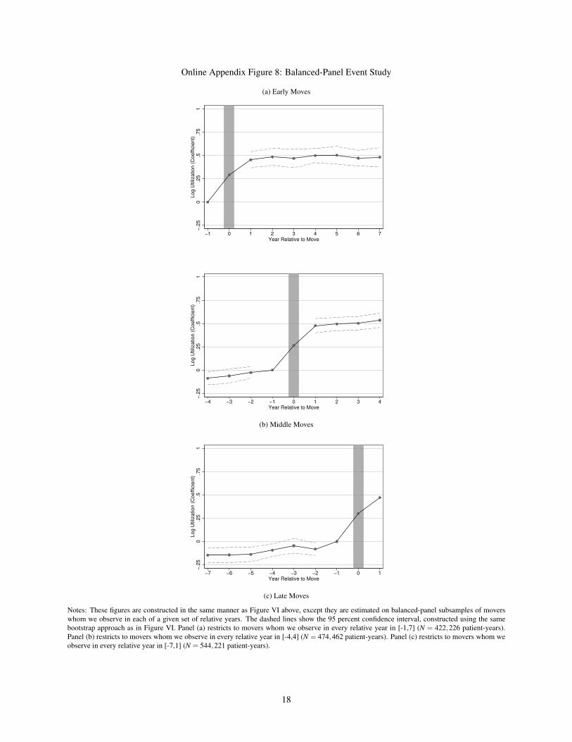
Online Appendix Table 9 presents a number of additional robustness checks. We estimate the model using onlymovers, without the age controls and relative year fixed effects ρr(i,t) in xit . We use alternative dependent variables:expenditure rather than utilization, and the log of 10 plus utilization or 0.1 plus utilization rather than 1 plus utilization.We drop moves to Florida, Arizona, and California. We estimate equation (2) using the balanced panel samples fromOnline Appendix Figure 8. In all these cases, the results remain similar in magnitude.

Online Appendix Figure 8 presents three alternative event-study plots using balanced panels. Panel (a) restricts thesample to early movers for whom we have data for relative years -1 through 7, using only these years in estimation.Panels (b) and (c) are analogous, restricting the sample to movers with data for relative years -4 through 4 and -7through 1 respectively. The balanced panel figures suggest if anything a slightly larger patient share, and confirm thefinding of a small pre-trend and no post-trend.

4.5 Empirical Bayes Adjustment for Event Study

Figure VI in the main text presents event-study estimates of equation (6). To account for noise in estimating δi,in Online Appendix Figure 7 we apply an Empirical Bayes (EB) adjustment procedure to these estimates as in Morris(1983). Specifically, we compute for each HRR j a convex combination of the estimated y j terms and the overall meanof log utilization across HRRs, which we denote y. The EB-adjusted estimates are given as

(12) yEBj =

(1− B j

)y j + B j y

where

(13) B j =

(NH −1−2

NH −1

)σ2

j

σ2j + σ2 .

σ2j is the standard error of the HRR mean y j, which is the within-HRR standard deviation divided by the square root

of the number of observations in the HRR. σ2 is the weighted average of squared deviations of the y j terms from y lessthe weighted average of the σ2

j terms. σ2 is computed from the following equations through an iterative procedure.

σ2 = max

0,∑ j Wj

{(NH

NH−1

)(y j− y)2− σ2

j

}∑ j Wj

(14)

Wj =1

σ2j + σ2(15)

We iterate the weight W until we obtain a stable σ2 term. NH = 306, the number of HRRs.Once we have the estimates yEB

j for each HRR j, we can compute δ EBi for each patient i as follows,

(16) δEBi = δi = yEB

d(i)− yEBo(i)

Then we estimate the event-study regression shown in equation (17), and plot the coefficients on the θr(i,t)δEBi terms.

(17) yit = αi +θr(i,t)δEBi + τt + xitβ + εit

We use the following posterior distribution for the yEBj terms when computing bootstrapped standard errors:

(18) N(yEB

j , σ2j(1− B j

)).

12

ReferencesCard, David, Joerg Heining, and Patrick M. Kline. 2013. “Workplace Heterogeneity and the Rise of West German

Wage Inequality.” Quarterly Journal of Economics, 128(3): 967–1015.

Centers for Medicare and Medicaid Services. 2014. “Medicare Claims Processing Manual.” Centers for Medicareand Medicaid Services.

Charlson, Mary E., Peter Pompei, Kathy L. Ales, and C. Ronald MacKenzie. 1987. “A New Method of Classify-ing Prognostic Comorbidity in Longitudinal Studies: Development and Validation.” Journal of Chronic Diseases,40(5): 373–383.

Cutler, David, Jonathan Skinner, Ariel Dora Stern, and David Wennberg. 2015. “Physician Beliefs and PatientPreferences: A New Look at Regional Variation in Health Care Spending.” Harvard Business School Working Paper15-090.

Gottlieb, Daniel J., Weiping Zhou, Yunjie Song, Kathryn G. Andrews, Jonathan S. Skinner, and Jason M.Sutherland. 2010. “Prices Don’t Drive Regional Medicare Spending Variations.” Health Affairs, 29(3): 537–543.

Health and Retirement Study. 2014. Restricted data public use datasets. Produced and distributed by the Universityof Michigan with funding from the National Institute on Aging (grant number NIA U01AG009740), Ann Arbor,MI, 2014.

Iezzoni, Lisa I., Timothy Heeren, Susan M. Foley, Jennifer Daley, John Hughes, and Gerald A. Coffman. 1994.“Chronic Conditions and Risk of in-Hospital Death.” Health Services Research, 29(4): 435–460.

Morris, Carl N. 1983. “Parametric Empirical Bayes Inference: Theory and Applications.” Journal of the AmericanStatistical Association, 78(391): 47–55.

Newhouse, Joseph P., and Alan M. Garber. 2013. “Geographic Variation in Medicare Services.” New EnglandJournal of Medicine, 368(16): 1465–1468.

Pope, Gregory C., John Kautter, Randall P. Ellis, Arlene S. Ash, John Z. Ayanian, Lisa I. Iezzoni, Melvin J.Ingber, Jesse M. Levy, and John Robst. 2004. “Risk Adjustment of Medicare Capitation Payments Using theCMS-HCC Model.” Health Care Financing Review, 25(4): 119–141.

Song, Yunjie, Jonathan Skinner, Julie Bynam, Jason Sutherland, and Elliott Fisher. 2010. “Regional Variationsin Diagnostic Practices.” New England Journal of Medicine, 363(1): 45–53.

13

Online Appendix Figure 1: Event Study of Log Number of Chronic Conditions

−.2

50

.25

.5.7

51

Ln(#

of C

hro

nic

Conditio

ns +

1)

(Coeffic

ient)

−10 −9 −8 −7 −6 −5 −4 −3 −2 −1 0 1 2 3 4 5 6 7 8 9Year Relative to Move

Notes: Figure is constructed in the same manner as Figure VI, except that it uses the log number of chronic conditions as the dependent variable.The dashed lines show the 95 percent confidence interval, constructed using the same bootstrap approach as in Figure VI. The sample includes allmover-years except 1998, as chronic conditions are not observed in that year (N = 3,407,590 patient-years).

14

Online Appendix Figure 2: Distribution of Distance Moved

0.0

5.1

.15

.2S

hare

of M

overs

0 1000 2000 3000 4000 5000Distance Moved (Miles)

Mean: 588.4SD: 615.6 Q1: 119.8Median: 356.5Q3: 913.2

Notes: Figure shows the distribution of distances moved. Distance is measured between the population-weighted centroids of HRRs. The sample isall movers (N = 497,097 patients).

Online Appendix Figure 3: Distribution of the Number of Movers Across Destination HRRs

135 − 535535 − 873873 − 13771377 − 23832383 − 12797

Notes: Map shows the distribution of the number of movers in different destinations in quintiles. Lower and upper limits of each quintile aredisplayed in the legend. The sample is all movers (N = 497,097 patients).

15

Online Appendix Figure 4: Log Utilization Over Relative Years

6.5

77.5

8Log U

tiliz

ation

−10 −9 −8 −7 −6 −5 −4 −3 −2 −1 0 1 2 3 4 5 6 7 8 9Relative Year

Mean Log Utilization of Movers

Mean Log Utilization of Matched Non−Movers

Notes: Figure shows the mean log utilization by relative year for movers and a matched sample of non-movers. In Figure IV, we describe theconstruction of a matched sample of non-movers from the mover’s origin HRR; we construct an analogous sample of non-movers in the mover’sdestination HRR. For each relative year, we compute the mean of log utilization each matched sample of non-movers, and take the average of thetwo. The sample is all movers (N = 3,702,189 patient-years) and the same number of non-mover patient-years.

Online Appendix Figure 5: HRS Top Reasons for Move

Near/with children

Other

Health problem/services

Near/with relatives/friends

Smaller/less expensive home

Work/retirement

Climate or weatherMarital status change

30.56%

26.37%

13.12%

9.601%

7.032%

4.936%

4.26%4.124%

Notes: Pie chart shows the most common reasons for moving, based on the HRS. Reasons mentioned fewer than 50 times are grouped under the“Other” category. Of the 2,025 movers in the data, 1,144 provide reasons; some provide multiple. The sample is all reasons given (N = 1,479observations).

16

Online Appendix Figure 6: Share of Claims in Destination (All Address Changers)

0.2

5.5

.75

1S

hare

of C

laim

s in D

estination H

RR


Notes: Figure displays the mean share of claims in the destination HRR by relative year. Here, we categorize someone as a mover if their HRR ofresidence changes exactly once (N = 5,698,027 patient-years). By contrast, in our baseline definition we apply the additional sample restrictionthat movers must also increase the share of claims in their destination HRR, among claims in either their origin or destination HRR, by at least 0.75in the post-move years relative to the pre-move years.

Online Appendix Figure 7: Event Study with Empirical Bayes Adjustment

−.2

50

.25

.5.7

51

Log U

tiliz

ation (

Coeffic

ient)


Standard Event Study EB Adjusted Event Study

Notes: The EB adjusted event study is shown superimposed over the standard event study from Figure VI. The EB adjusted event study isconstructed in the same manner as Figure VI, except the estimates of δi are adjusted using the empirical Bayes (EB) procedure. The dashed linesshow the 95 percent confidence interval, constructed using the same bootstrap approach as in Figure VI. The sample is all movers (N = 3,702,189patient-years).

17

Online Appendix Figure 8: Balanced-Panel Event Study

(a) Early Moves

−.2

50

.25

.5.7

51

Log U

tiliz

ation (

Coeffic

ient)

−1 0 1 2 3 4 5 6 7Year Relative to Move

−.2

50

.25

.5.7

51

Log U

tiliz

ation (

Coeffic

ient)

−4 −3 −2 −1 0 1 2 3 4Year Relative to Move

(b) Middle Moves

−.2

50

.25

.5.7

51

Log U

tiliz

ation (

Coeffic

ient)

−7 −6 −5 −4 −3 −2 −1 0 1Year Relative to Move

(c) Late Moves

Notes: These figures are constructed in the same manner as Figure VI above, except they are estimated on balanced-panel subsamples of moverswhom we observe in each of a given set of relative years. The dashed lines show the 95 percent confidence interval, constructed using the samebootstrap approach as in Figure VI. Panel (a) restricts to movers whom we observe in every relative year in [-1,7] (N = 422,226 patient-years).Panel (b) restricts to movers whom we observe in every relative year in [-4,4] (N = 474,462 patient-years). Panel (c) restricts to movers whom weobserve in every relative year in [-7,1] (N = 544,221 patient-years).

18

Online Appendix Figure 9: Time Series of Mean Log Utilization of HRRs by Quintile

6.5

77.5

8M

ean L

og U

tiliz

ation

1998 2000 2002 2004 2006 2008Observation Year

Notes: Figure displays a time series plot of the mean log utilization for each HRR quintile and year. HRR quintiles are defined by taking the averageacross individuals within each HRR-year, up-weighting non-movers by four, and then taking the simple average within HRR across years. Thesample is all movers (N = 3,702,189 patient-years).

19

Online Appendix Figure 10: Event-Study Results for Various Components of Utilization

(a) Seen a Primary Care Physician−

.25

0.2

5.5

.75

11.2

5S

een a

Prim

ary

Care

Physic

ian (

Coeffic

ient)


(b) Seen a Specialist

−.2

50

.25

.5.7

51

1.2

5S

een a

Specia

list (C

oeffic

ient)


−.2

50

.25

.5.7

51

1.2

5A

ny H

ospitaliz

ation (

Coeffic

ient)


(c) Any Hospitalization

−.2

50

.25

.5.7

51

1.2

5A

ny E

merg

ency R

oom

Utiliz

ation (

Coeffic

ient)


(d) Any Emergency Room Utilization

−.2

50

.25

.5.7

51

1.2

5Ln(#

of dia

gnostic tests

+1)

(Coeffic

ient)


(e) Log Number of Diagnostic Tests

−.2

50

.25

.5.7

51

1.2

5Ln(#

of im

agin

g tests

+1)

(Coeffic

ient)


(f) Log Number of Imaging Tests

20

−.2

50

.25

.5.7

51

1.2

5Ln(#

of P

reventive C

are

Measure

s+

1)

(Coeffic

ient)


(g) Log Number of Preventive Care Measures

−.2

50

.25

.5.7

51

1.2

5Ln(#

of docto

rs+

1)

(Coeffic

ient)


(h) Log Number of Different Doctors Seen

−.2

50

.25

.5.7

51

1.2

5Ln(I

npatient R

BU

+1)

(Coeffic

ient)


(i) Log Inpatient Utilization

−.2

50

.25

.5.7

51

1.2

5Ln(O

utp

atient R

BU

+1)

(Coeffic

ient)


(j) Log Outpatient Utilization

−.2

50

.25

.5.7

51

1.2

5Ln(E

merg

ency R

oom

RB

U +

1)

(Coeffic

ient)


(k) Log Emergency Room Utilization

−.2

50

.25

.5.7

51

1.2

5Ln(O

ther

RB

U +

1)

(Coeffic

ient)


(l) Log Other Utilization

Notes: These figures are constructed in the same manner as Figure VI, except the dependent variable is now an alternate utilization measure. Thedashed lines show the 95 percent confidence interval, constructed using the same bootstrap approach as in Figure VI. All log outcome measuresare the log of the outcome plus one. Online Appendix Table 11 shows the percent with zero for each of these outcomes. The sample is all movers(N = 3,702,189 patient-years).

21

Online Appendix Figure 11: Event Study, Moves Up and Moves Down

(a) Moves from Low to High-Utilization HRRs

−.2

50

.25

.5.7

51

Log U

tiliz

ation (

Coeffic

ient)


−.2

50

.25

.5.7

51

Log U

tiliz

ation (

Coeffic

ient)


(b) Moves from High to Low-Utilization HRRs

Notes: These figures are constructed in the same manner as Figure VI, except they are estimated on moves up in panel (a) and on moves down inpanel (b). A move up is defined to be a move to a destination HRR with higher mean log utilization than the mean log utilization of the origin. Amove down is defined to be a move to a destination HRR with lower mean log utilization than the mean log utilization of the origin. The dashedlines show the 95 percent confidence interval, constructed using the same bootstrap approach as in Figure VI. The sample in panel (a) is all moverswho move up (N = 1,792,033 patient-years). The sample in panel (b) is all movers who move down (N = 1,910,156 patient-years).

22

Online Appendix Figure 12: Event Study, Results By Age Quartile−

.25

0.2

5.5

.75

1Log U

tiliz

ation (

Coeffic

ient)


(a) Age Quartile 1

−.2

50

.25

.5.7

51

Log U

tiliz

ation (

Coeffic

ient)


(b) Age Quartile 2

−.2

50

.25

.5.7

51

Log U

tiliz

ation (

Coeffic

ient)


(c) Age Quartile 3

−.2

50

.25

.5.7

51

Log U

tiliz

ation (

Coeffic

ient)


(d) Age Quartile 4

Notes: These figures are constructed in the same manner as Figure VI, except that they are estimated on subsamples of all movers divided by agequartiles. Quartiles of age are determined based on the mean age over the years observed for each patient. Panel (a) provides estimates for thefirst quartile of age (mean age 68.5), panel (b) provides estimates for the second quartile of age (mean age 72.8), panel (c) provides estimates forthe third quartile of age (mean age 78.3), and panel (d) provides estimates for the fourth quartile of age (mean age 86.1). The dashed lines showthe 95 percent confidence interval, constructed using the same bootstrap approach as in Figure VI. The sample in panel (a) includes movers in thefirst quartile of age (N = 746,132 patient-years); panel (b) includes movers in the second quartile (N = 868,531 patient-years); panel (c) includesmovers in the third quartile (N = 977,512 patient-years); panel (d) includes movers in the fourth quartile (N = 1,110,014 patient-years).

23

Online Appendix Figure 13: Event Study for Robustness Specifications

(a) First Third of Sample Only (1998-2001)

−.2

50

.25

.5.7

51

Log U

tiliz

ation (

Coeffic

ient)

−3 −2 −1 0 1 2 3Year Relative to Move

(b) Second Third of Sample Only (2002-2005)

−.2

50

.25

.5.7

51

Log U

tiliz

ation (

Coeffic

ient)


(c) Third Third of Sample Only (2006-2008)

−.2

50

.25

.5.7

51

Log U

tiliz

ation (

Coeffic

ient)


(d) Patients Who Never Die

−.2

50

.25

.5.7

51

Log U

tiliz

ation (

Coeffic

ient)


(e) Patients Never in an HMO

−.2

50

.25

.5.7

51

Log U

tiliz

ation (

Coeffic

ient)


(f) Patients Never Missing Outcomes

−.2

50

.25

.5.7

51

Log U

tiliz

ation (

Coeffic

ient)


24

−.2

50

.25

.5.7

51

Log U

tiliz

ation (

Coeffic

ient)


(g) Analysis at State Level

−.2

50

.25

.5.7

51

Log U

tiliz

ation (

Coeffic

ient)


(h) Analysis at Hospital Service Area (HSA) Level

−.2

50

.25

.5.7

51

Log U

tiliz

ation (

Coeffic

ient)


(i) Limit to Cross State Movers

−.2

50

.25

.5.7

51

Log U

tiliz

ation (

Coeffic

ient)


(j) Limit to Cross Census Region Movers

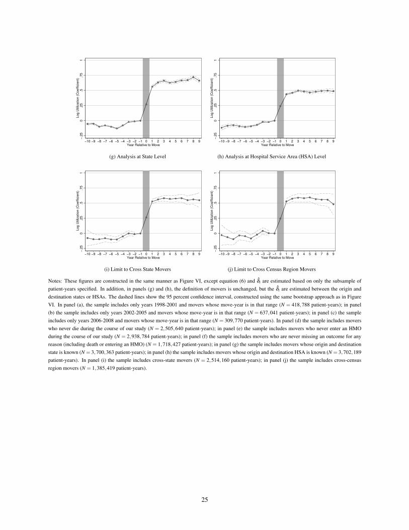
Notes: These figures are constructed in the same manner as Figure VI, except equation (6) and δi are estimated based on only the subsample ofpatient-years specified. In addition, in panels (g) and (h), the definition of movers is unchanged, but the δi are estimated between the origin anddestination states or HSAs. The dashed lines show the 95 percent confidence interval, constructed using the same bootstrap approach as in FigureVI. In panel (a), the sample includes only years 1998-2001 and movers whose move-year is in that range (N = 418,788 patient-years); in panel(b) the sample includes only years 2002-2005 and movers whose move-year is in that range (N = 637,041 patient-years); in panel (c) the sampleincludes only years 2006-2008 and movers whose move-year is in that range (N = 309,770 patient-years). In panel (d) the sample includes moverswho never die during the course of our study (N = 2,505,640 patient-years); in panel (e) the sample includes movers who never enter an HMOduring the course of our study (N = 2,938,784 patient-years); in panel (f) the sample includes movers who are never missing an outcome for anyreason (including death or entering an HMO) (N = 1,718,427 patient-years); in panel (g) the sample includes movers whose origin and destinationstate is known (N = 3,700,363 patient-years); in panel (h) the sample includes movers whose origin and destination HSA is known (N = 3,702,189patient-years). In panel (i) the sample includes cross-state movers (N = 2,514,160 patient-years); in panel (j) the sample includes cross-censusregion movers (N = 1,385,419 patient-years).

25

Online Appendix Figure 14: Event-Study Analysis of Level Utilization and Percentile of Utilization

(a) Level Utilization

−.2

50

.25

.5.7

51

1.2

51.5

Utiliz

ation (

Coeffic

ient)


(b) Percentile of Utilization

−.2

50

.25

.5.7

51

1.2

51.5

Perc

entile

of U

tiliz

ation (

Coeffic

ient)


Notes: These figures are constructed in the same manner as Figure VI , except in panel (a) the dependent variable is level utilization and in panel (b)the dependent variable is percentile of utilization. The dashed lines show the 95 percent confidence interval, constructed using the same bootstrapapproach as in Figure VI. The sample is all movers (N = 3,702,189 patient-years).

26

Online Appendix Figure 15: Event-Study Results for Health Measures

−.2

50

.25

.5.7

51

Ln(H

CC

Com

munity S

core

) (C

oeffic

ient)


(a) Log HCC Score, All Moves

−.2

50

.25

.5.7

51

Ln(#

of Ie

zzoni C

hro

nic

Conditio

ns+

1)

(Coeffic

ient)


(b) Log Iezzoni Chronic Conditions, All Moves

−.2

50

.25

.5.7

51

Ln(C

harlson C

om

orb

idity Index+

1)

(Coeffic

ient)


(c) Log Charlson Comorbidity Index, All Moves

27

−.2

50

.25

.5.7

51

Ln(H

CC

Com

munity S

core

) (C

oeffic

ient)


(d) Log HCC Score. Early Moves. Moves Up.

−.2

50

.25

.5.7

51

Ln(H

CC

Com

munity S

core

) (C

oeffic

ient)


(e) Log HCC Score. Early Moves. Moves Down.

−.2

50

.25

.5.7

51

Ln(C

harlson C

om

orb

idity Index+

1)

(Coeffic

ient)


(f) Log Charlson Comorbidity Index. Early Moves. Moves Up.

−.2

50

.25

.5.7

51

Ln(C

harlson C

om

orb

idity Index+

1)

(Coeffic

ient)


(g) Log Charlson Comorbidity Index. Early Moves. Moves Down.

−.2

50

.25

.5.7

51

Ln(#

of Ie

zzoni C

hro

nic

Conditio

ns+

1)

(Coeffic

ient)


(h) Log Iezzoni Chronic Conditions. Early Moves. Moves Up.

−.2

50

.25

.5.7

51

Ln(#

of Ie

zzoni C

hro

nic

Conditio

ns+

1)

(Coeffic

ient)


(i) Log Iezzoni Chronic Conditions. Early Moves. Moves Down.

Notes: These figures are constructed in the same manner as Figure VI, except the dependent variables are various health measures and they areestimated on balanced-panel subsamples of movers whom we observe in each of a given set of relative years. The dashed lines show the 95 percentconfidence interval, constructed using the same bootstrap approach as in Figure VI. All log outcome measures are the log of the outcome plus one,except the HCC score which is bounded away from 0. Online Appendix Table 11 shows the percent with zero for each of these outcomes. In panels(a)-(c) the sample is all movers (N = 3,702,189 patient-years). In panels (d), (f), and (h), the sample is movers whom we observe in every relativeyear in [-1,7] and who move to higher utilization areas (N = 212,958 patient-years). In panels (e), (g), and (i), the sample is movers whom weobserve in every relative year in [-1,7] and who move to lower utilization areas (N = 209,268 patient-years).

28

Online Appendix Figure 16: Event Study with Non-Movers Included

−.2

50

.25

.5.7

51

Log U

tiliz

ation (

Coeffic

ient)


Standard Event Study Include Non−Movers

Notes: The event study including non-movers is shown superimposed over the standard event study from Figure VI. The event study with non-movers is constructed in the same manner as Figure VI except for non-movers we adapt equation 5, setting δi to zero and o(i) to patient i’s areaof residence. This yields an event-study equation similar to equation 6, with δi equal to zero for non-movers. The dashed lines show the 95percent confidence interval, constructed using the same bootstrap approach as in Figure VI. In the standard event study, the sample is all movers(N = 3,702,189 patient-years). When we include non-movers, the sample is all movers and non-movers (N = 16,432,955 patient-years).

29

Online Appendix Figure 17: Lasso: Covariates of Place Effects

0.0 0.1 0.2 0.3 0.4 0.5

−0.0

50.0

00.0

50.1

0

L1 Norm

Coeffic

ients

0 9 16 21 21 25

Percent Female

Adjusted Log Chronic Conditions

Adjusted Log Iezzoni

Hospital Beds Per Capita

Non−Profit Hospitals

High follow−up PCP

Comforter PCP

Cowboy Cardiologists

Notes: This figure shows the paths of the Lasso coefficients as the penalty bound is varied. Each line represents a coefficient plotted as a functionof the L1 norm of the set of coefficients, illustrating the set of covariates that would have been chosen for various penalty levels. The dashed lineindicates the model selected by minimizing the mean-squared error when performing 10-fold cross-validation. Each variable is standardized to havemean zero and a standard deviation of one prior to performing Lasso.

30

Online Appendix Figure 18: Lasso: Covariates of Patient Effects

0.0 0.1 0.2 0.3 0.4

−0.0

4−

0.0

20.0

00.0

20.0

40.0

6

L1 Norm

Coeffic

ients

0 7 15 20 26

Percent Black

Percent Female

Average Education

Adjusted Log Chronic Conditions

Adjusted Log Charlson

Adjusted Log Iezzoni

Have Unneeded Tests

Aggressive Patient

Comforter Patient

Hospital Compare ScorePCP Per Capita

Hospital Beds Per Capita

Non−Profit Hospitals

High follow−up PCP

Low follow−up PCP

Cowboy PCP

High Follow−up Cardiologists Low Follow−up Cardiologists

Cowboy Cardiologists

Notes: This figure shows the paths of the Lasso coefficients as the penalty bound is varied. Each line represents a coefficient plotted as a functionof the L1 norm of the set of coefficients, illustrating the set of covariates that would have been chosen for various penalty levels. The dashed lineindicates the model selected by minimizing the mean-squared error when performing 10-fold cross-validation. Each variable is standardized to havemean zero and a standard deviation of one prior to performing Lasso.

31

Online Appendix Figure 19: Event-Study Analysis for Moves Across Specific Geographic Areas

(a) Above and Below Median−

.75

−.5

−.2

50

.25

.5.7

51

1.2

51.5

Log U

tiliz

ation (

Coeffic

ient)


(b) Top and Bottom Quartiles

−.7

5−

.5−

.25

0.2

5.5

.75

11.2

51.5

Log U

tiliz

ation (

Coeffic

ient)


(c) Top and Bottom 10 Percent

−.7

5−

.5−

.25

0.2

5.5

.75

11.2

51.5

Log U

tiliz

ation (

Coeffic

ient)


(d) Top and Bottom 5 Percent

−.7

5−

.5−

.25

0.2

5.5

.75

11.2

51.5

Log U

tiliz

ation (

Coeffic

ient)


Notes: These figures are constructed in the same manner as Figure VI, except that they are estimated on the sample of moves between areas in thegiven percentiles of average utilization. The dashed lines show the 95 percent confidence interval constructed using the same bootstrap approachas in Figure VI. The samples in panels (a), (b), (c), and (d) are all movers who move between areas with above median and below median averageutilization (N = 1,386,791), all movers who move between areas in the top quartile and the bottom quartile of average utilization (N = 275,638),all movers who move between areas in the top 10 percent and bottom 10 percent of average utilization (N = 40,328), and all movers who movebetween areas in the top 5 percent and the bottom 5 percent of average utilization (N = 13,102), respectively. These correspond to the movesanalyzed in columns (1) through (4), respectively, of Table II

32

Online Appendix Table 1: Movements Between Census Divisions (Movers Only, as Percentage of All Moves)

Destination

ENC ESC M-A M NE P SA WNC WSC Total

Origin

East North Central 7.00 0.94 0.32 0.91 0.14 0.65 2.53 0.63 0.73 13.86

East South Central 0.65 1.56 0.10 0.14 0.04 0.15 1.13 0.14 0.49 4.40

Mid-Atlantic 0.58 0.28 6.26 0.53 0.92 0.56 5.57 0.15 0.36 15.21

Mountain 0.62 0.17 0.20 2.64 0.10 1.58 0.57 0.65 0.75 7.29

New England 0.15 0.08 0.40 0.19 1.56 0.21 1.54 0.05 0.10 4.26

Pacific 0.53 0.28 0.26 2.74 0.14 9.04 0.93 0.51 1.00 15.43

South Atlantic 2.51 1.59 2.71 0.77 1.06 0.84 13.12 0.50 1.00 24.10

West North Central 0.52 0.15 0.07 0.63 0.04 0.36 0.47 2.44 0.66 5.35

West South Central 0.54 0.55 0.14 0.65 0.07 0.59 0.85 0.62 6.08 10.10

Total 13.12 5.60 10.47 9.21 4.08 13.97 26.73 5.69 11.18 100.00

Notes: Table shows the percentage of moves that take place between each of the 81 origin-destination pairs of census divisions. The denominatoris all movers (N = 497,097 patients).

33

Online Appendix Table 2: HRS Summary Statistics

(1) (2)Non-movers Movers

Average age over observed waves 74.93 77.03Average age in first observed wave 70.65 72.26Average age in 1992 64.60 68.23Female 0.55 0.60White 0.81 0.89Hispanica 0.08 0.04

EducationLess than high school 0.33 0.26GED 0.04 0.04High school 0.30 0.31Some college 0.18 0.20College 0.15 0.19

Retirement status (in first observed wave)b

Retired 0.51 0.51Partly retired 0.16 0.15Retired or partly retired 0.66 0.66

Earnings (in first observed wave)c

Average $5,803 $5,115Average conditional on positive $22,641 $21,505Median conditional on positive $13,000 $13,000Share with zero 0.67 0.79

Marital status (in first observed wave)Married or partnered 0.66 0.63Separated or divorced 0.08 0.09Widowed 0.23 0.27Never married 0.03 0.01

# of patients 20,998 2,025# of patient-years 83,202 11,068

aThere are three race categories in the data: White/Caucasian, Black/African-American, and Other. Hispanic is a separate variable, so someone canappear as White and Hispanic, Black and Hispanic, White and Non-Hispanic, etc.

bRespondents are asked whether they consider themselves retired. They can have the following non-missing responses: not retired, completelyretired, and partly retired.cThe sum of respondent’s wage/salary income, bonuses/overtime pay/commissions/tips, second job or military reserve earnings, professional prac-tice or trade income.

34

Online Appendix Table 3: HRS Summary of Regression Results

(1) (2) (3)Row Xit # patient-

waves% moves

in thesample

Estimatedcoefficient

(standard error)

(1) Unmarried & unpartnered 81,613 0.0192 0.0122 (0.0026)(2) Separated/divorced 81,613 0.0192 0.0033 (0.0050)(3) Widowed 81,613 0.0192 0.0094 (0.0025)(4) Retired or partly retired 66,472 0.0204 0.0035 (0.0019)(5) Poor/fair Health 94,270 0.0215 -0.0021 (0.0015)

Notes: Table shows the coefficients and standard errors from estimating the regression in Online Appendix equation (4) for each of the indicatorvariables in the rows of the table. For each row, column (1) shows the number of patient-waves for which the indicator variable is not missing.Column (2) shows the fraction of patient-waves counted in column (1) in which a move happens. Column (3) shows results from estimating a linearregression with wave fixed effects and person fixed effects. Because of missing data, rows have different sample sizes (column (1)) and slightlydifferent percentages moving (column (2)).

35

Online Appendix Table 4: Robustness

(1) (2) (3) (4)Specification N Mean of log

utilizationAbove / below medianutilization difference

Share dueto patients

(1) Baseline 16,031,875 7.193 0.283 0.465

(2) Relative years -5 to 5 15,430,835 7.193 0.283 0.469(3) Relative years -3 to 3 14,689,929 7.193 0.283 0.499(4) Relative years -1 to 1 13,511,698 7.192 0.284 0.557

(5) First third of sample only (1998-2001) 4,857,799 6.936 0.284 0.490(6) Second third of sample only (2002-2005) 5,238,278 7.252 0.290 0.519(7) Third third of sample only (2006-2008) 3,599,208 7.452 0.303 0.621

(8) First differences with fixed effects 16,432,955 7.197 0.281 0.583

(9) HRR fixed effects interacted with age quartiles 16,031,875 7.193 0.283 0.441

(10) Patients who never die 10,999,832 6.904 0.292 0.527(11) Patients never in an HMO 13,432,817 7.224 0.284 0.468(12) Patients never missing outcomes 8,135,140 6.921 0.287 0.509

(13) Using states as geographic unit 16,029,246 7.146 0.282 0.446(14) Using HSAs as geographic unit 16,031,875 7.201 0.391 0.561

(15) Cross state movers only 14,974,181 7.192 0.283 0.451(16) Cross census region movers only 13,967,660 7.190 0.284 0.451

Notes: Table reports the share of the difference in utilization between above and below median HRRs due to patients, analogous to column (1)of Table II, for alternative samples and specifications. Columns report the sample size, mean of log utilization, difference in average utilizationbetween above and below median utilization HRRs (yR− yR′ ) and patient share (Spat (R,R′)). Rows (2) to (4) narrow the sample of years for moversto relative years -5 to 5, relative years -3 to 3, and relative years -1 to 1, respectively. Rows (5)-(7) limit the sample to patient years in 1998-2001,2002-2005, and 2006-2008, respectively, excluding movers whose move year falls outside the time window in question. In row (8) we estimate themodel in first differences, allowing for patient and place-specific trends in log utilization (see equation 5); here we do not drop the year of the move(relative year 0), but use the adjustment technique described in Online Appendix Section 4.3 assuming that there is no misreporting in move timingother than a 50 percent chance of a patient being in their origin in relative year zero and a 50 percent chance of a patient being in their destinationin relative year 0. In row (9), we add interaction terms between HRR dummies and dummies for age quartiles. Rows (10), (11), and (12) restrictthe sample to patients who do not die in sample, who are never in an HMO, and who never have a missing value of utilization for any reason,respectively. Rows (13) and (14) change the geographic of unit of analysis to states and Hospital Service Areas (HSAs), respectively. We do notchange our sample selection criteria for movers when we vary the definition of the geographic unit j in the model. In row (13), the sample size fallsslightly because there is a small number of patients for whom we do not have a valid state code. Rows (15) and (16) restrict the sample of moversto those who cross state or census region boundaries, respectively.

36

Online Appendix Table 5: Additive Decomposition (Estimation in Logs, Decomposition in Levels)

(1) (2) (3) (4) (5) (6)Above / below

medianTop &

bottom 25%Top &

bottom 10%Top &

bottom 5%McAllen &

El PasoMiami &

Minneapolis

Difference in mean predicted utilizationOverall 807 1,294 1,768 2,074 2,053 3,692If we equalize patient effects 592 898 1,159 1,319 1,340 1,790If we equalize place effects 228 410 605 749 551 1,493

Slevelpat (R,R′) 0.267 0.306 0.345 0.364 0.347 0.515

(0.041) (0.036) (0.041) (0.045) (0.214) (0.054)Slevel

place (R,R′) 0.718 0.683 0.658 0.639 0.732 0.596

(0.041) (0.038) (0.045) (0.049) (0.183) (0.060)

Notes: Table based on estimation of equation (2); the estimates are transformed based on Online Appendix equations (6), (7), and (8). The measuresreported in this table are explained in Online Appendix Section 4.2. Each column defines a set of areas R and R′. The first row reports the differencein average predicted level utilization overall between the two sets ( ¯yR− ¯yR′ ); the second row reports the difference in predicted level utilization thatwould remain if we counterfactually equalized patient effects ( ¯yR,pateq− ¯yR′,pateq); the third row reports the difference in predicted level utilizationthat would remain if we counterfactually equalized place effects ( ¯yR,pleq− ¯yR′,pleq). The fourth row reports the share of difference in predicted levelutilization due to patients. The fifth row reports the share of the difference in predicted level utilization due to place. Standard errors (in parentheses)are calculated using a bootstrap procedure with 50 repetitions at the patient level. In columns (1)-(4), the partitions of places shown in the columnsare defined based on average utilization in each HRR. The sample size is the same as in Table II.

Online Appendix Table 6: Alternative Definitions of Movers

(1) (2) (3) (4)Mover definition Mean of

log uti-lization

Above /below

medianutilizationdifference


N (% of movers retained)

(1) Baseline 7.193 0.283 0.465 16,031,875 (100%)(2) Looser claim share criterion (0.6) 7.195 0.282 0.489 16,250,644 (106%)(3) Stricter claim share criterion (0.9) 7.190 0.284 0.443 15,659,995 (90.5%)(4) No claim share criterion 7.199 0.282 0.592 17,792,048 (153%)(5) Baseline, adjusted for move timing measurement error 7.193 0.283 0.444 16,031,875 (100%)(6) Include multiple movers 7.193 0.282 0.474 16,322,118 (102%)

Notes: Table reports the share of the difference in utilization between above and below median HRRs due to patients, analogous to column (1) ofTable II, for alternative samples and specifications. Columns report the mean of log utilization, difference in average utilization between above andbelow median utilization HRRs , patient share (Spat (R,R′)), and sample size and percent of movers retained. Row (1) repeats our baseline results.

Row (2): We modify the baseline definition to categorize someone as a mover if their HRR of residence changes and their average claim share inthe destination HRR increases by at least 0.6 instead of 0.75; the remainder of the definition remains unchanged.

Row (3): We modify the baseline definition to categorize someone as a mover if their HRR of residence changes and their average claim share inthe destination HRR increases by at least 0.9 instead of 0.75; the remainder of the definition remains unchanged.

Row (4): We categorize someone as a mover if their HRR of residence changes.

Row (5): Same as Row (1), but we adjust for measurement error in move timing by estimating Online Appendix equation (11).

Row (6): We modify the baseline definition to include movers who change their HRR of residence more than once.

37

Online Appendix Table 7: Narrow Window Specifications for Components of Utilization

(1) (2)Utilization Measure Share due to

patientsShare due to Patients,Relative Years -1 to 1

(1) Baseline: Log(utilization) 0.465 0.557

(2) Seen a primary care physician 0.452 0.547(3) Seen a specialist 0.322 0.390(4) Any hospitalization 0.410 0.376(5) Any emergency room visit 0.714 0.679

(6) Log (# of diagnostic tests) 0.092 0.129(7) Log(# of imaging tests) 0.142 0.176(8) Log(# of preventive care measures)a 0.611 0.652(9) Log(# of different doctors seen) 0.392 0.467

(10) Log(inpatient utilization)b 0.242 0.195(11) Log(outpatient utilization)b 0.358 0.406(12) Log(emergency room utilization)b 0.639 0.662(13) Log(other utilization)b 0.124 0.145

Notes: Table reports the share of the difference in utilization between above and below median HRRs due to patients, analogous to column (1)of Table II, for alternative samples and specifications. Column (1) reports the share of the difference in the average utilization measure betweenabove and below median HRRs that is due to patients (Spat (R,R′)). Column (2) reports this same share, but narrows the sample of movers used forestimation to relative years -1 and +1. All log outcome measures are the log of the outcome plus 1. The partition of HRRs into above and belowmedian groups is based on the utilization of individuals in the baseline sample and differs in each row according to the definition of utilizationused; it is computed separately for each column. Online Appendix Table 11 shows the percent with zero for each of these outcomes. The samplesize is the same as in Table II in column (1). In column (2), the sample is all non-movers and mover relative years -1 and +1 (N = 13,511,698patient-years).a“# of preventive care measures” includes how many of the following treatments the patient received in the past year: Ambulatory Care, EyeScreening, Hemoglobin Test, Lipid Screen, Cardio Screen, Diabetes Management, Pelvic Screen, Bone Mass Test, Colorectal Cancer Screening,Flu Shot, or in the past two years: Mammogram, Pap Test, and Prostate Cancer Screening.

38

Online Appendix Table 8: Alternative Measures of Utilization

(1) (2) (3)Outcome Mean of

outcomeAbove / below mediandifference in outcome


(1) Utilization (in levels) 6629.120 1231.389 0.228(2) Percentile in national distribution 49.791 3.694 0.295(3) In top 80% of utilization 0.791 0.048 0.505(4) In top 50% of utilization 0.484 0.059 0.252(5) In top 20% of utilization 0.195 0.032 0.317(6) In top 10% of utilization 0.097 0.022 0.165(7) In top 5% of utilization 0.048 0.014 0.225

Notes: Table reports the share of the difference in utilization between above and below median HRRs due to patients, analogous to column (1) ofTable II, for alternative samples and specifications. Columns report the mean of log utilization, difference in average utilization between above andbelow median utilization HRRs (yR− yR′ ) and patient share (Spat (R,R′)). In row (1), the outcome is level utilization. In row (2), the outcome isthe percentile of the national distribution of utilization that a patient is in. In rows (3) to (7), the outcome is an indicator for being in the top 80percent, 50 percent, 20 percent, 10 percent, and 5 percent, respectively, of the national distribution of utilization. The partition of HRRs into aboveand below median groups is based on the utilization of individuals in the baseline sample and differs in each row according to the definition ofutilization used. The sample size is the same as in Table II.

Online Appendix Table 9: Additional Robustness Checks

(1) (2) (3) (4)Specification N Mean of log

utilizationAbove / below medianutilization difference


(1) Baseline 16,031,875 7.193 0.283 0.465

(2) Movers only 3,301,109 7.252 0.287 0.481(3) Drop age as a covariate 16,031,875 7.193 0.283 0.446(4) Drop relative year as a covariate 16,031,875 7.193 0.283 0.485

(5) Log(total expenditure) 16,031,875 7.156 0.291 0.453(6) Log(utilization+0.1) 16,031,875 7.062 0.326 0.508(7) Log(utilization+10) 16,031,875 7.339 0.243 0.360

(8) Drop moves to Florida 15,640,033 7.193 0.282 0.447(9) Drop moves to Florida, Arizona, and California 15,250,903 7.192 0.283 0.428

(10) Early moves 13,106,078 7.190 0.284 0.453(11) Middle moves 13,152,510 7.190 0.284 0.456(12) Late moves 13,214,518 7.190 0.284 0.532

Notes: Table reports the share of the difference in utilization between above and below median HRRs due to patients, analogous to column (1)of Table II, for alternative samples and specifications. Columns report the sample size, mean of log utilization, difference in average utilizationbetween above and below median utilization HRRs (yR− yR′ ) and patient share (Spat (R,R′)). Row (2) only uses movers when estimating equation(2). Row (3) drops age as a covariate when estimating equation (2) and row (4) drops relative year when estimating equation (2). Rows (5) to (7)change the outcome variable to the log of total expenditures, the log of utilization + 0.1, and the log of utilization + 10, respectively. Rows (8) and(9) drop moves to Florida and to Florida, Arizona, and California, respectively. Row (10) includes movers only if they are observed continuously ineach relative year in [-1,7] and all non-movers; row (11) includes movers only if they are observed continuously in each relative year [-4,4] and allnon-movers; row (12) includes movers only if they are observed continuously in each relative year [-7,1] and all non-movers.

39

Online Appendix Table 10: Additive Decomposition of Health Outcomes

(1) (2) (3) (4) (5) (6)Outcome Mean of Difference in average outcome Share of

differenceShare of

differenceOutcome Overall Due to

patientsDue toplace

due topatients

due to place

(1) Log(HCC score) -0.132 0.115 0.056 0.059 0.485 0.515(2) Log(Charlson Comorbidity Index) 0.672 0.102 0.044 0.058 0.430 0.570(3) Log(Iezzoni chronic conditions) 0.495 0.100 0.042 0.058 0.418 0.582(4) Log(# of chronic conditions) 1.181 0.138 0.059 0.079 0.430 0.570

Notes: Table reports the share of the difference in utilization between above and below median HRRs due to patients and places, analogous tocolumn (1) of Table II, for alternative dependent variables. Columns report the mean of the dependent variable, difference in the average outcomebetween above and below median utilization HRRs, the difference due to place (γR− γR′ ), the difference due to patients (y∗R− y∗R′ ), the patient share(Spat (R,R′)), and the place share (Splace (R,R′)). HRRs are partitioned into above and below median places based on the average of the givenoutcome (by row) in each HRR. All log outcome measures are the log of the outcome plus one, except the HCC score which is bounded away fromzero. Online Appendix Table 11 shows the percent with zero for each of these outcomes. The sample size is the same as in Table II in rows (1)-(3).In row (4), the sample also excludes the year 1998, as chronic conditions are not observed in that year (N = 14,598,443 patient-years).

Online Appendix Table 11: Share Zero for Components of Utilization and Health Measures

(1) (2)Non-Movers Movers

(1) # of diagnostic tests 0.33 0.30(2) # of imaging tests 0.45 0.42(3) # of preventive care measures 0.10 0.09(4) # of different doctors seen 0.07 0.07

(5) Inpatient utilization 0.75 0.74(6) Outpatient utilization 0.07 0.07(7) Emergency room utilization 0.71 0.69(8) Other utilization 0.35 0.31

(9) Charlson Comorbity Index 0.16 0.14(10) # of Iezzoni Chronic Conditions 0.41 0.40(11) # of Chronic Conditions 0.49 0.47

# of patient-years 12,730,766 3,702,189

Notes: We report the share of patient-years for which the utilization component or health measure has a value of zero. We use the log of thesemeasures plus one in Tables IV and V, Online Appendix Tables 7 and 10, and Online Appendix Figures 10 and 15. The sample is all movers andnon-movers (N = 16,432,955 patient-years).

40

Online Appendix Table 12: HRR-level Patient and Place Covariate Summary Statistics

(1) (2)Mean Standard Deviation

Medicare dataPatient demographics

Average age 76.0 (0.6)Percent black 0.084 (0.081)Percent female 0.589 (0.017)

Patient healthAdjusted Log HCC score -0.163 (0.046)Adjusted Log Chronic Conditions 1.236 (0.042)Adjusted Log Charlson 0.654 (0.034)Adjusted Log Iezzoni 0.500 (0.038)

Census dataMedian household income (thousands) 49.090 (13.997)High school completion rate 0.838 (0.041)

Patient PreferencesHave unneeded tests 0.715 (0.146)See unneeded cardiologist 0.548 (0.174)Aggressive patient preferences ratio 0.066 (0.076)Comfort patient preferences ratio 0.513 (0.160)

Physician PreferencesPCPs

High follow-up 0.026 (0.058)Low follow-up 0.069 (0.134)Cowboy 0.223 (0.237)Comforter 0.513 (0.275)

CardiologistsHigh follow-up 0.184 (0.237)Low follow-up 0.013 (0.055)Cowboy 0.248 (0.249)Comforter 0.292 (0.263)

Hospital Compare ScorePercent timely and effective care 80.385 (3.8)

Physician prevalenceSpecialists per thousand residents 2.633 (1.051)PCPs per thousand residents 1.190 (0.313)

Hospital characteristicsHospital beds per thousand residents 3.174 (0.869)Percent non-profit hospitals 0.805 (0.159)

Notes: Table reports the mean and standard deviation (shown in parentheses) of each correlate of the patient and place effects outlined in Appendix3.2. These statistics are computed among N = 96 HRRs, comprising about 60 percent of our baseline sample.

41

Online Appendix Table 13: Correlates of Patient and Place Fixed Effects Using All 306 HRRs

(1) (2) (3) (4)Patient Effects Place Effects

306 HRRs 96 HRRs 306 HRRs 96 HRRs

Patient demographics

Average Age -0.008 0.034 0.011(0.014) (0.014) (0.014)

Percent Black -0.011 0.008(0.009) (0.010)

Percent Female 0.034 0.006 0.008(0.014) (0.011) (0.018)

Patient SES

Median household income 0.006 -0.013 -0.019(0.006) (0.016) (0.011)

High school completion rate 0.044 0.046 -0.028 -0.009(0.007) (0.009) (0.010) (0.016)

Patient health

Adjusted Log HCC Score -0.088(0.023)

Adjusted Log Chronic Conditions 0.058 0.052 0.045 0.041(0.009) (0.022) (0.016) (0.025)

Adjusted Log Charlson 0.030 -0.009(0.009) (0.022)

Adjusted Log Iezzoni 0.030 0.052 -0.002(0.024) (0.020) (0.031)

Provider characteristics

Percent timely and effective care 0.005 0.011 0.019(0.024) (0.006) (0.010)

Specialists per thousand residents 0.008(0.014)

PCPs per thousand residents 0.032 0.014 0.017 -0.037(-0.019) (0.011) (0.016) (0.027)

Beds per thousand residents -0.013 -0.043 0.023 0.028(0.006) (0.011) (0.009) (0.017)

Percent non-profit hospitals -0.009 -0.032 -0.037 -0.041(0.006) (0.011) (0.008) (0.014)

Observations 306 96 306 96R2 0.530 0.631 0.300 0.286

Notes: Table reports the correlates of the patient (columns (1) and (2)) and place effects (columns (3) and (4)). Columns (1) and (3) report resultsfrom post-Lasso regression on all 306 HRRs. Columns (2) and (4) report results from post-Lasso on the 96 HRRs with non-missing measures forpatient preferences and provider styles. All covariates have been standardized to have mean zero with a standard deviation of one. Robust standarderrors are reported in parentheses.

42

Documents

Sources of Geographic Variation in Health Care