Embed Size (px)
Citation preview

Communications in Mathematical Finance, vol.1, no.1, 2012, 51-74
ISSN: 2241-1968 (print), 2241-195X (online)
Scienpress Ltd, 2012
Some Numerical Methods for
Options Valuation
C.R. Nwozo1 and S.E. Fadugba2
Abstract
Numerical Methods form an important part of options valuation
and especially in cases where there is no closed form analytic formula.
We discuss three numerical methods for options valuation namely Bi-
nomial model, Finite difference methods and Monte Carlo simulation
method. Then we compare the convergence of these methods to the
analytic Black-Scholes price of the options. Among the methods con-
sidered, Crank Nicolson finite difference method is unconditionally sta-
ble, more accurate and converges faster than binomial model and Monte
Carlo Method when pricing vanilla options, while Monte carlo simula-
tion method is good for pricing path dependent options.
Mathematics Subject Classification:65C05, 91G60, 60H30, 65N06
Keywords: Binomial model, Finite difference method,
Monte Carlo simulation method, Real Options
1 Department of Mathematics, University of Ibadan, Nigeria,
e-mail: [email protected] Department of Mathematical and Physical Sciences, Afe Babalola University,
Ado Ekiti, Nigeria, e-mail: [email protected]
Article Info: Received : July 3, 2012. Revised : August 6, 2012
Published online : August 10, 2012
52 Some Numerical Methods for Options Valuation
1 Introduction
Numerical methods are needed for pricing options in cases where analytic
solutions are either unavailable or not easily computable. Examples of the
former include American style options and most discretely observed path de-
pendent options, while the latter includes the analytic formula for valuing
continuously observed Asian options which is very hard to calculate for a wide
range of parameter values encountered in practice.
The subject of numerical methods in the area of options valuation and
hedging is very broad. A wide range of different types of contracts are avail-
able and in many cases there are several candidate models for the stochastic
evolution of the underlying state variables [13].
Now, we present an overview of three popular numerical methods available
in the context of Black-Scholes-Merton [2, 8] for vanilla and path dependent
options valuation which are binomial model for pricing options based on risk-
neutral valuation derived by Cox-Ross-Rubinstein [6], finite difference methods
for pricing derivative governed by solving the underlying partial differential
equations was considered by Brennan and Schwarz [5] and Monte Carlo ap-
proach introduced by Boyle [3] for pricing European option and path dependent
options. The comparative study of finite difference method and Monte Carlo
method for pricing European option was considered by [9]. These procedures
provide much of the infrastructure in which many contributions to the field
over the past three decades have been centered.
2 Numerical Methods for Options Valuation
This section presents three numerical methods for options valuation namely:
• Binomial Methods.
• Finite Difference Methods.
• Monte Carlo Methods.

C.R. Nwozo and S.E. Fadugba 53
2.1 Binomial Model
This is defined as an iterative solution that models the price evolution
over the whole option validity period. For some types of options such as the
American options, using an iterative model is the only choice since there is no
known closed form solution that predicts price over time. Black-Scholes model
seems dominated the option pricing, but it is not the only popular model, the
Cox-Ross-Rubinstein (CRR) “Binomial” model has a large popularity. The
binomial model was first suggested by Cox-Ross-Rubinstein model in paper
“Option Pricing: A Simplified Approach” [6] and assumes that stock price
movements are composed of a large number of small binomial movements. The
Cox-Ross-Rubinstein model [7] contains the Black-Scholes analytical formula
as the limiting case as the number of steps tends to infinity.
We know that after one time period, the stock price can move up to Su
with probability p or down to Sd with probability (1 − p). Therefore the
corresponding value of the call option at the first time movement δt is given
by
fu = max(Su−K, 0) (1)
fd = max(Sd−K, 0) (2)
where fu and fd are the values of the call option after upward and downward
movements respectively.
We need to derive a formula to calculate the fair price of the option. The
risk neutral call option price at the present time is
f = e−rδt[pfu + (1− p)fd] (3)
where the risk neutral probability is given by
p =erδt − d
u− d(4)
Now, we extend the binomial model to two periods. Let fuu denote the
call value at time 2δt for two consecutive upward stock movement, fud for one
downward and one upward movement and fdd for two consecutive downward
movement of the stock price. Then we have
fuu = max(Suu−K, 0) (5)

54 Some Numerical Methods for Options Valuation
fud = max(Sud−K, 0) (6)
fdd = max(Sdd−K, 0 (7)
The values of the call options at time δt are
fu = e−rδt[pfuu + (1− p)fud] (8)
fd = e−rδt[pfud + (1− p)fdd] (9)
Substituting (8) and (9) into (3), we have
f = e−rδt[pe−rδt(pfuu + (1− p)fud) + (1− p)e−rδt(pfud + (1− p)fdd)]
f = e−2rδt[
p2fuu + 2p(1− p)fud + (1− p)2fdd]
(10)
(10) is called the current call value using time 2δt, where the numbers p2,
2p(1 − p) and (1 − p)2 are the risk neutral probabilities that the underlying
asset prices Suu, Sud and Sdd respectively are attained.
We generalize the result in (10) to value an option at T = Nδt as
f = e−Nrδt
N∑
j=0
(Nj )pj(1− p)N−jfujdN−j
f = e−Nrδt
N∑
j=0
(
Nj
)
pj(1− p)N−j max(SujdN−j −K, 0) (11)
where fujdN−j = max(SujdN−j − K, 0) and(
Nj
)
= N !(N−j)!j!
is the binomial
coefficient . We assume that m is the smallest integer for which the option’s
intrinsic value in (11) is greater than zero. This implies that SumdN−m ≥ K.
Then (11) is written as
f = Se−Nrδt
N∑
j=0
(
Nj
)
pj(1− p)N−jujdN−j
−Ke−Nrδt
N∑
j=0
(
Nj
)
pj(1− p)N−j (12)
which gives us the present value of the call option.
The term e−Nrδt is the discounting factor that reduces f to its present
value. The first term(
Nj
)
pj (1− p)N−j is the binomial probability of j up-
ward movements to occur after the first N trading periods and SujdN−j is the
corresponding value of the asset after j upward move of the stock price.
C.R. Nwozo and S.E. Fadugba 55
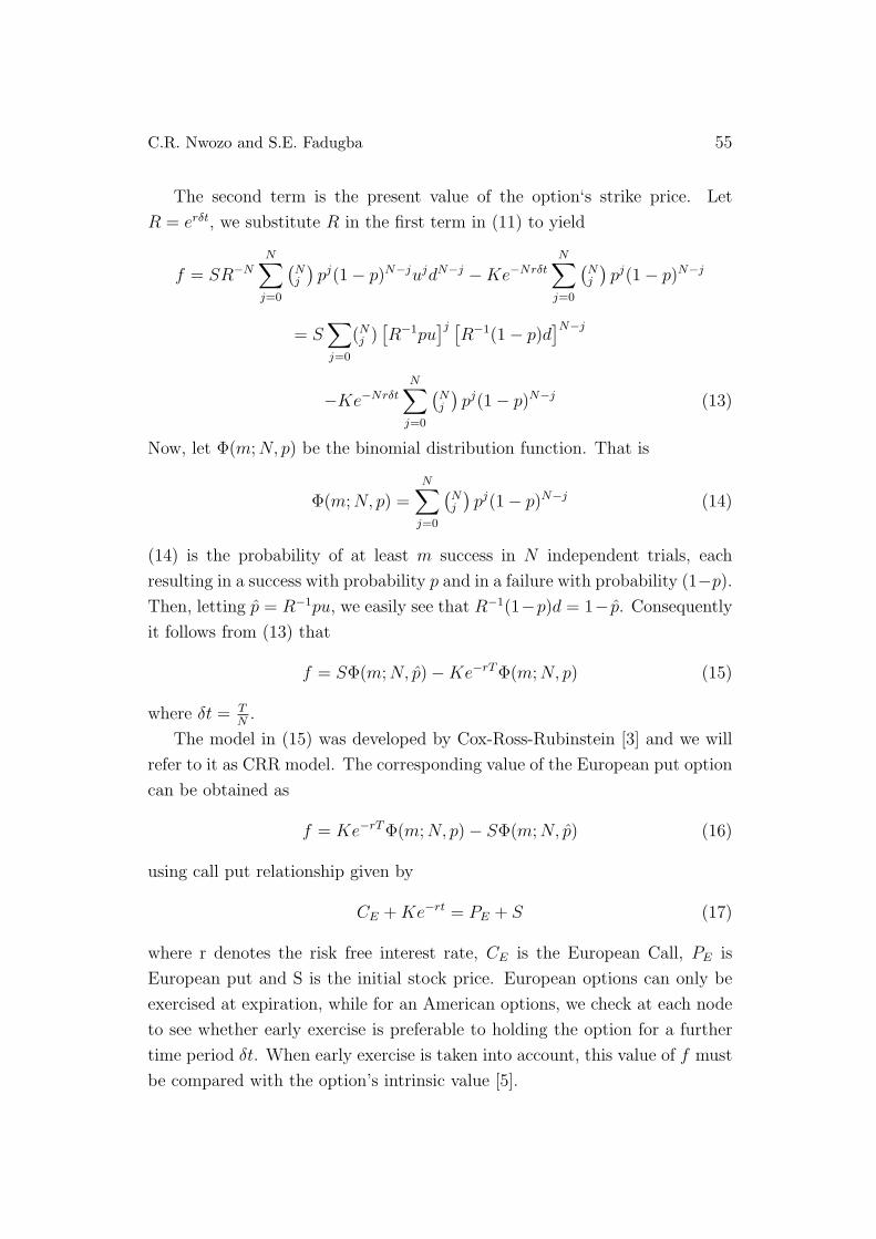
The second term is the present value of the option‘s strike price. Let
R = erδt, we substitute R in the first term in (11) to yield
f = SR−N
N∑
j=0
(
Nj
)
pj(1− p)N−jujdN−j −Ke−Nrδt
N∑
j=0
(
Nj
)
pj(1− p)N−j
= S∑
j=0
(Nj )[
R−1pu]j [
R−1(1− p)d]N−j
−Ke−Nrδt
N∑
j=0
(
Nj
)
pj(1− p)N−j (13)
Now, let Φ(m;N, p) be the binomial distribution function. That is
Φ(m;N, p) =N∑
j=0
(
Nj
)
pj(1− p)N−j (14)
(14) is the probability of at least m success in N independent trials, each
resulting in a success with probability p and in a failure with probability (1−p).
Then, letting p̂ = R−1pu, we easily see that R−1(1−p)d = 1− p̂. Consequently
it follows from (13) that
f = SΦ(m;N, p̂)−Ke−rTΦ(m;N, p) (15)
where δt = TN.
The model in (15) was developed by Cox-Ross-Rubinstein [3] and we will
refer to it as CRR model. The corresponding value of the European put option
can be obtained as
f = Ke−rTΦ(m;N, p)− SΦ(m;N, p̂) (16)
using call put relationship given by
CE +Ke−rt = PE + S (17)
where r denotes the risk free interest rate, CE is the European Call, PE is
European put and S is the initial stock price. European options can only be
exercised at expiration, while for an American options, we check at each node
to see whether early exercise is preferable to holding the option for a further
time period δt. When early exercise is taken into account, this value of f must
be compared with the option’s intrinsic value [5].
56 Some Numerical Methods for Options Valuation
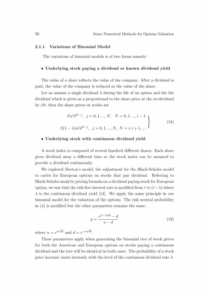
2.1.1 Variations of Binomial Model
The variations of binomial models is of two forms namely:
• Underlying stock paying a dividend or known dividend yield
The value of a share reflects the value of the company. After a dividend is
paid, the value of the company is reduced so the value of the share.
Let us assume a single dividend λ during the life of an option and the the
dividend which is given as a proportional to the share price at the ex-dividend
by iδt, then the share prices at nodes are
SujdN−j, j = 0, 1, ..., N, N = 0, 1, ..., i− 1
S(1− λ)ujdN−j, j = 0, 1, ..., N, N = i, i+ 1, ...
}
(18)
• Underlying stock with continuous dividend yield
A stock index is composed of several hundred different shares. Each share
gives dividend away a different time so the stock index can be assumed to
provide a dividend continuously.
We explored Merton’s model, the adjustment for the Black-Scholes model
to carter for European options on stocks that pay dividend. Referring to
Black-Scholes analytic pricing formula on a dividend paying stock for European
option, we saw that the risk-free interest rate is modified from r to (r−λ) where
λ is the continuous dividend yield [14]. We apply the same principle in our
binomial model for the valuation of the options. The risk neutral probability
in (4) is modified but the other parameters remains the same.
p =e(r−λ)δt − d
u− d(19)
where u = eσ√δt and d = e−σ
√δt.
These parameters apply when generating the binomial tree of stock prices
for both the American and European options on stocks paying a continuous
dividend and the tree will be identical in both cases. The probability of a stock
price increase varies inversely with the level of the continuous dividend rate λ.
C.R. Nwozo and S.E. Fadugba 57
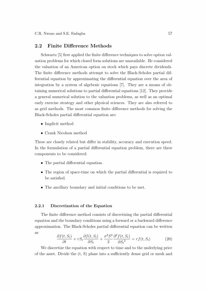
2.2 Finite Difference Methods
Schwartz [5] first applied the finite difference techniques to solve option val-
uation problems for which closed form solutions are unavailable. He considered
the valuation of an American option on stock which pays discrete dividends.
The finite difference methods attempt to solve the Black-Scholes partial dif-
ferential equation by approximating the differential equation over the area of
integration by a system of algebraic equations [7]. They are a means of ob-
taining numerical solutions to partial differential equations [12]. They provide
a general numerical solution to the valuation problems, as well as an optimal
early exercise strategy and other physical sciences. They are also referred to
as grid methods. The most common finite difference methods for solving the
Black-Scholes partial differential equation are:
• Implicit method
• Crank Nicolson method
These are closely related but differ in stability, accuracy and execution speed.
In the formulation of a partial differential equation problem, there are three
components to be considered:
• The partial differential equation.
• The region of space-time on which the partial differential is required to
be satisfied.
• The ancillary boundary and initial conditions to be met.
2.2.1 Discretization of the Equation
The finite difference method consists of discretizing the partial differential
equation and the boundary conditions using a forward or a backward difference
approximation. The Black-Scholes partial differential equation can be written
as∂f(t, St)
∂t+ rSt
∂f(t, St)
∂St
+σ2S2
2
∂2f(t, St)
∂St2 = rf(t, St) (20)
We discretize the equation with respect to time and to the underlying price
of the asset. Divide the (t, S) plane into a sufficiently dense grid or mesh and
58 Some Numerical Methods for Options Valuation
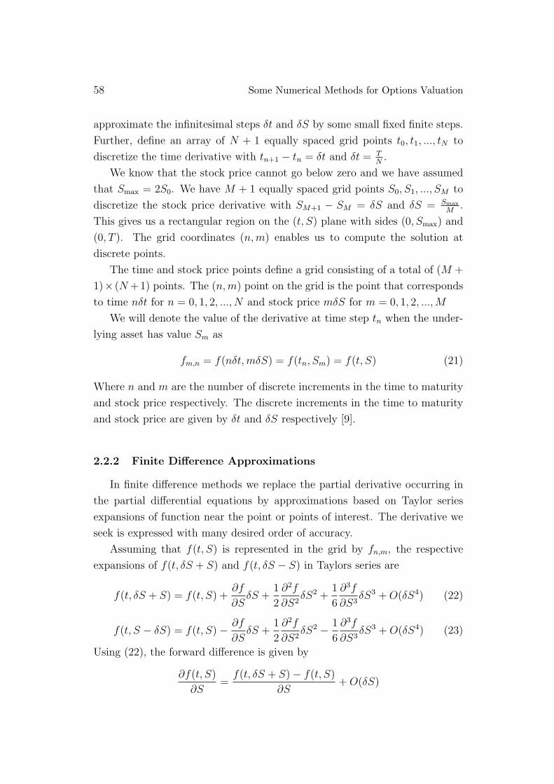
approximate the infinitesimal steps δt and δS by some small fixed finite steps.
Further, define an array of N + 1 equally spaced grid points t0, t1, ..., tN to
discretize the time derivative with tn+1 − tn = δt and δt = TN.
We know that the stock price cannot go below zero and we have assumed
that Smax = 2S0. We have M + 1 equally spaced grid points S0, S1, ..., SM to
discretize the stock price derivative with SM+1 − SM = δS and δS = Smax
M.
This gives us a rectangular region on the (t, S) plane with sides (0, Smax) and
(0, T ). The grid coordinates (n,m) enables us to compute the solution at
discrete points.
The time and stock price points define a grid consisting of a total of (M +
1)× (N +1) points. The (n,m) point on the grid is the point that corresponds
to time nδt for n = 0, 1, 2, ..., N and stock price mδS for m = 0, 1, 2, ...,M
We will denote the value of the derivative at time step tn when the under-
lying asset has value Sm as
fm,n = f(nδt,mδS) = f(tn, Sm) = f(t, S) (21)
Where n and m are the number of discrete increments in the time to maturity
and stock price respectively. The discrete increments in the time to maturity
and stock price are given by δt and δS respectively [9].
2.2.2 Finite Difference Approximations
In finite difference methods we replace the partial derivative occurring in
the partial differential equations by approximations based on Taylor series
expansions of function near the point or points of interest. The derivative we
seek is expressed with many desired order of accuracy.
Assuming that f(t, S) is represented in the grid by fn,m, the respective
expansions of f(t, δS + S) and f(t, δS − S) in Taylors series are
f(t, δS + S) = f(t, S) +∂f
∂SδS +
1
2
∂2f
∂S2δS2 +
1
6
∂3f
∂S3δS3 +O(δS4) (22)
f(t, S − δS) = f(t, S)− ∂f
∂SδS +
1
2
∂2f
∂S2δS2 − 1
6
∂3f
∂S3δS3 +O(δS4) (23)
Using (22), the forward difference is given by
∂f(t, S)
∂S=
f(t, δS + S)− f(t, S)
∂S+O(δS)
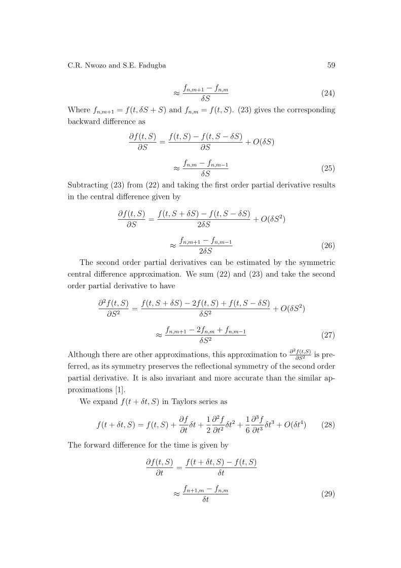
C.R. Nwozo and S.E. Fadugba 59
≈ fn,m+1 − fn,m
δS(24)
Where fn,m+1 = f(t, δS + S) and fn,m = f(t, S). (23) gives the corresponding
backward difference as
∂f(t, S)
∂S=
f(t, S)− f(t, S − δS)
∂S+O(δS)
≈ fn,m − fn,m−1
δS(25)
Subtracting (23) from (22) and taking the first order partial derivative results
in the central difference given by
∂f(t, S)
∂S=
f(t, S + δS)− f(t, S − δS)
2δS+O(δS2)
≈ fn,m+1 − fn,m−1
2δS(26)
The second order partial derivatives can be estimated by the symmetric
central difference approximation. We sum (22) and (23) and take the second
order partial derivative to have
∂2f(t, S)
∂S2=
f(t, S + δS)− 2f(t, S) + f(t, S − δS)
δS2+O(δS2)
≈ fn,m+1 − 2fn,m + fn,m−1
δS2(27)
Although there are other approximations, this approximation to ∂2f(t,S)∂S2 is pre-
ferred, as its symmetry preserves the reflectional symmetry of the second order
partial derivative. It is also invariant and more accurate than the similar ap-
proximations [1].
We expand f(t+ δt, S) in Taylors series as
f(t+ δt, S) = f(t, S) +∂f
∂tδt+
1
2
∂2f
∂t2δt2 +
1
6
∂3f
∂t3δt3 +O(δt4) (28)
The forward difference for the time is given by
∂f(t, S)
∂t=
f(t+ δt, S)− f(t, S)
δt
≈ fn+1,m − fn,m
δt(29)
60 Some Numerical Methods for Options Valuation
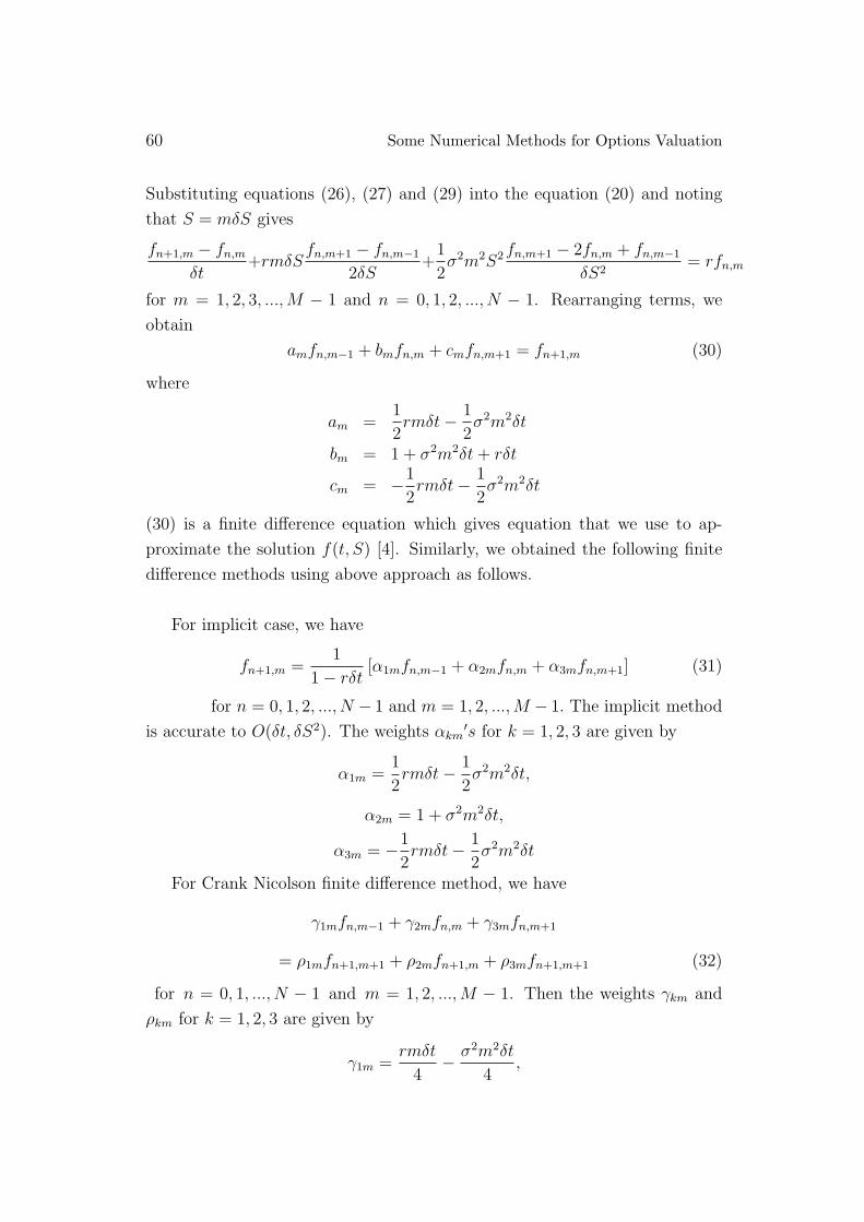
Substituting equations (26), (27) and (29) into the equation (20) and noting
that S = mδS gives
fn+1,m − fn,m
δt+rmδS
fn,m+1 − fn,m−1
2δS+1
2σ2m2S2fn,m+1 − 2fn,m + fn,m−1
δS2= rfn,m
for m = 1, 2, 3, ...,M − 1 and n = 0, 1, 2, ..., N − 1. Rearranging terms, we
obtain
amfn,m−1 + bmfn,m + cmfn,m+1 = fn+1,m (30)
where
am =1
2rmδt− 1
2σ2m2δt
bm = 1 + σ2m2δt+ rδt
cm = −1
2rmδt− 1
2σ2m2δt
(30) is a finite difference equation which gives equation that we use to ap-
proximate the solution f(t, S) [4]. Similarly, we obtained the following finite
difference methods using above approach as follows.
For implicit case, we have
fn+1,m =1
1− rδt[α1mfn,m−1 + α2mfn,m + α3mfn,m+1] (31)
for n = 0, 1, 2, ..., N − 1 and m = 1, 2, ...,M − 1. The implicit method
is accurate to O(δt, δS2). The weights αkm′s for k = 1, 2, 3 are given by
α1m =1
2rmδt− 1
2σ2m2δt,
α2m = 1 + σ2m2δt,
α3m = −1
2rmδt− 1
2σ2m2δt
For Crank Nicolson finite difference method, we have
γ1mfn,m−1 + γ2mfn,m + γ3mfn,m+1
= ρ1mfn+1,m+1 + ρ2mfn+1,m + ρ3mfn+1,m+1 (32)
for n = 0, 1, ..., N − 1 and m = 1, 2, ...,M − 1. Then the weights γkm and
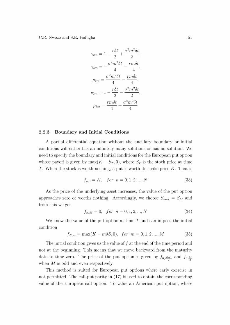
ρkm for k = 1, 2, 3 are given by
γ1m =rmδt
4− σ2m2δt
4,
C.R. Nwozo and S.E. Fadugba 61
γ2m = 1 +rδt
2+
σ2m2δt
2,
γ3m = −σ2m2δt
4− rmδt
4,
ρ1m =σ2m2δt
4− rmδt
4,
ρ2m = 1− rδt
2− σ2m2δt
2,
ρ3m =rmδt
4+
σ2m2δt
4
2.2.3 Boundary and Initial Conditions
A partial differential equation without the ancillary boundary or initial
conditions will either has an infinitely many solutions or has no solution. We
need to specify the boundary and initial conditions for the European put option
whose payoff is given by max(K − ST , 0), where ST is the stock price at time
T . When the stock is worth nothing, a put is worth its strike price K. That is
fn,0 = K, for n = 0, 1, 2, ..., N (33)
As the price of the underlying asset increases, the value of the put option
approaches zero or worths nothing. Accordingly, we choose Smax = SM and
from this we get
fn,M = 0, for n = 0, 1, 2, ..., N (34)
We know the value of the put option at time T and can impose the initial
condition
fN,m = max(K −mδS, 0), for m = 0, 1, 2, ...,M (35)
The initial condition gives us the value of f at the end of the time period and
not at the beginning. This means that we move backward from the maturity
date to time zero. The price of the put option is given by f0,M+1
2
and f0,M2
when M is odd and even respectively.
This method is suited for European put options where early exercise in
not permitted. The call-put parity in (17) is used to obtain the corresponding
value of the European call option. To value an American put option, where
62 Some Numerical Methods for Options Valuation
early exercised is permitted, we need to make only one simple modification [9].
After each linear system solution, we need to consider whether early exercise
is optimal or not. We compare fn,m with the intrinsic value of the option,
(K − mδS). If the intrinsic value is greater, then set fn,m to the intrinsic
value.
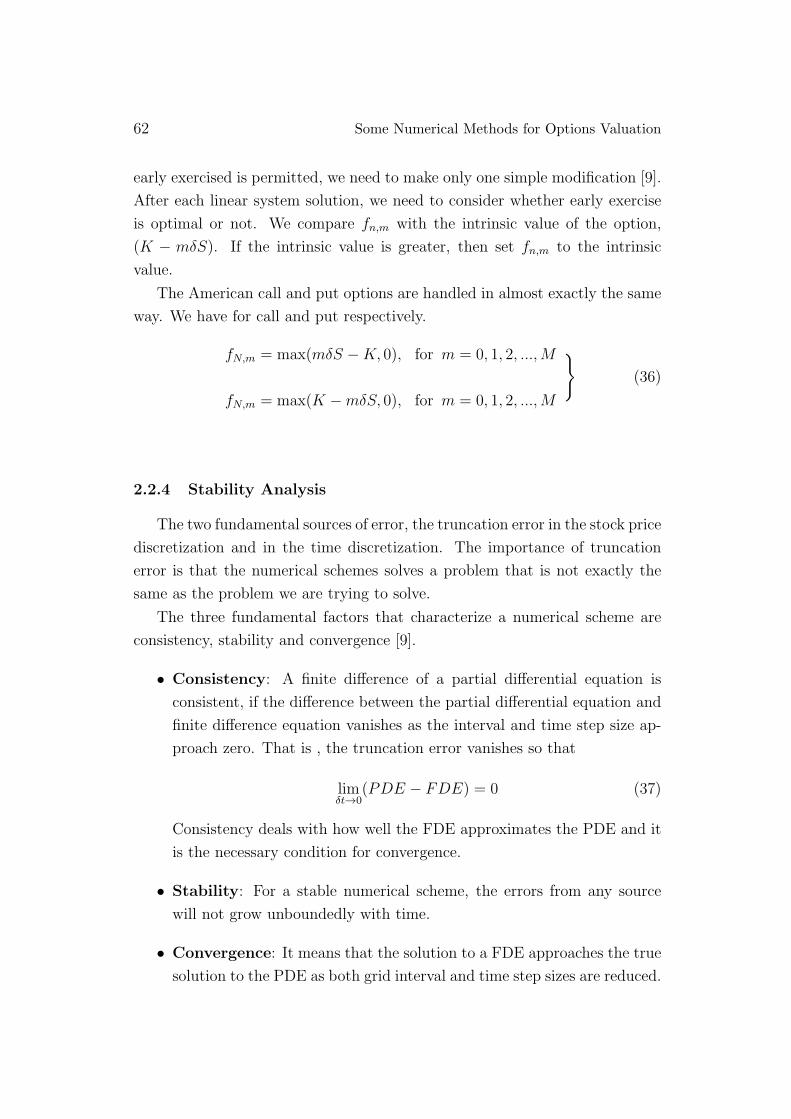
The American call and put options are handled in almost exactly the same
way. We have for call and put respectively.
fN,m = max(mδS −K, 0), for m = 0, 1, 2, ...,M
fN,m = max(K −mδS, 0), for m = 0, 1, 2, ...,M
}
(36)
2.2.4 Stability Analysis
The two fundamental sources of error, the truncation error in the stock price
discretization and in the time discretization. The importance of truncation
error is that the numerical schemes solves a problem that is not exactly the
same as the problem we are trying to solve.
The three fundamental factors that characterize a numerical scheme are
consistency, stability and convergence [9].
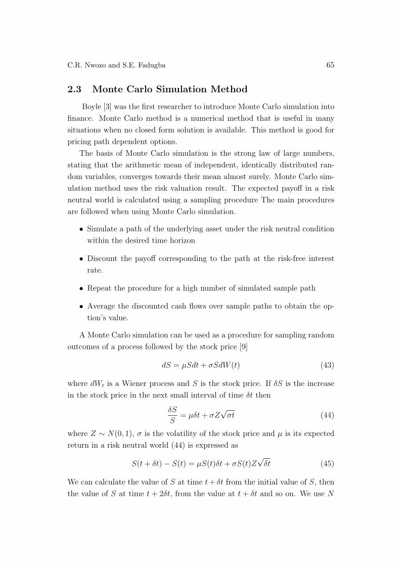
• Consistency: A finite difference of a partial differential equation is
consistent, if the difference between the partial differential equation and
finite difference equation vanishes as the interval and time step size ap-
proach zero. That is , the truncation error vanishes so that
limδt→0
(PDE − FDE) = 0 (37)
Consistency deals with how well the FDE approximates the PDE and it
is the necessary condition for convergence.
• Stability: For a stable numerical scheme, the errors from any source
will not grow unboundedly with time.
• Convergence: It means that the solution to a FDE approaches the true
solution to the PDE as both grid interval and time step sizes are reduced.

C.R. Nwozo and S.E. Fadugba 63
These three factors that characterize a numerical scheme are linked together
by Lax equivalence theorem [8] which states as follows;
Theorem 2.1. Given a well posed linear initial value problem and a consis-
tent finite difference scheme, stability is the necessary and sufficient condition
for convergence.
In general, a problem is said to be well posed if:
• a solution to the problem exists.
• the solution is unique when it exists.
• the solution depends continuously on the problem data.
2.2.5 A Necessary and Sufficient Condition for Stability
Let fn+1 = Afn be a system of equations. Matrix A and the column vectors
fn+1 and fn are as represented in (30). We have
fn = Afn−1
= A2fn−2
...
= Anf0
for n = 1, 2, ..., N (38)
where f0 is the vector of initial values. we are concerned with stability and
we investigate the propagation of a perturbation. Perturb the vector of initial
values f0 to f̂0. The exact solution at the nth time-row will then be
f̂n = Anf̂0 (39)
Let the perturbation or ‘error’ vector e be denoted by
e = f̂ − f
and using the perturbation vector (38) and (39) we have
en = f̂n − fn
= Anf̂0 − Anf0
= An(f̂0 − f0)

64 Some Numerical Methods for Options Valuation
Therefore,
en = Ane0, for n = 1, 2, ..., N (40)
Hence for compatible matrix and vector norms [8]
‖en‖ ≤ ‖An‖‖e0‖
Lax and Richmyer defined the difference scheme to be stable when there exists
a positive number L, independent of n, δt and δS such that
‖An‖ ≤ L, for n = 1, 2, ..., N
This limits the amplification of any initial perturbation and therefore of any
arbitrary initial rounding errors because it implies that
‖en‖ ≤ L‖e0‖
since ‖An‖ = ‖An−1A‖ ≤ ‖A‖‖An−1‖ ≤ · · · ≤ ‖A‖n, then the Lax-Richmyer
definition of stability is satisfied when
‖A‖ ≤ 1 (41)
condition (41) is the necessary and sufficient condition for the difference equa-
tions to be stable [8]. Since the spectral radius ρ(A) satisfies
ρ(A) ≤ ‖A‖
it follows automatically from (41) that
ρ(A) ≤ 1
We note that if matrix A is real and symmetric, then by definition [6], we
have
‖A‖∞ = moduli of the maximum row of matrix A
‖A‖2 = ρ(A) = max |λn| (42)
where λn is an eigenvalue of matrix A which is given by λn = y+2(√xz) cos nπ
N,
for n = 1, 2, ..., N where x, y and z are referred to as weights which may be
real or complex.
By Lax equivalence theorem, the two finite difference methods are consistent,
unconditionally stable and convergent.
C.R. Nwozo and S.E. Fadugba 65
2.3 Monte Carlo Simulation Method
Boyle [3] was the first researcher to introduce Monte Carlo simulation into
finance. Monte Carlo method is a numerical method that is useful in many
situations when no closed form solution is available. This method is good for
pricing path dependent options.
The basis of Monte Carlo simulation is the strong law of large numbers,
stating that the arithmetic mean of independent, identically distributed ran-
dom variables, converges towards their mean almost surely. Monte Carlo sim-
ulation method uses the risk valuation result. The expected payoff in a risk
neutral world is calculated using a sampling procedure The main procedures
are followed when using Monte Carlo simulation.
• Simulate a path of the underlying asset under the risk neutral condition
within the desired time horizon
• Discount the payoff corresponding to the path at the risk-free interest
rate.
• Repeat the procedure for a high number of simulated sample path
• Average the discounted cash flows over sample paths to obtain the op-
tion’s value.
A Monte Carlo simulation can be used as a procedure for sampling random
outcomes of a process followed by the stock price [9]
dS = µSdt+ σSdW (t) (43)
where dWt is a Wiener process and S is the stock price. If δS is the increase
in the stock price in the next small interval of time δt then
δS
S= µδt+ σZ
√σt (44)
where Z ∼ N(0, 1), σ is the volatility of the stock price and µ is its expected
return in a risk neutral world (44) is expressed as
S(t+ δt)− S(t) = µS(t)δt+ σS(t)Z√δt (45)
We can calculate the value of S at time t+ δt from the initial value of S, then
the value of S at time t + 2δt, from the value at t + δt and so on. We use N
66 Some Numerical Methods for Options Valuation
random samples from a normal distribution to simulate a trial for a complete
path followed by S. It is more accurate to simulate lnS than S, we transform
the asset price process using Ito’s lemma
d(lnS) =
(
µ− σ2
2
)
dt+ σdW (t)
so that
lnS(t+ δt)− lnS(t) =
(
µ− σ2
2
)
δt+ σZ√δt
or
S(t+ δt) = S(t) exp
[(
µ− σ2
2
)
δt+ σZ√δt
]
(46)
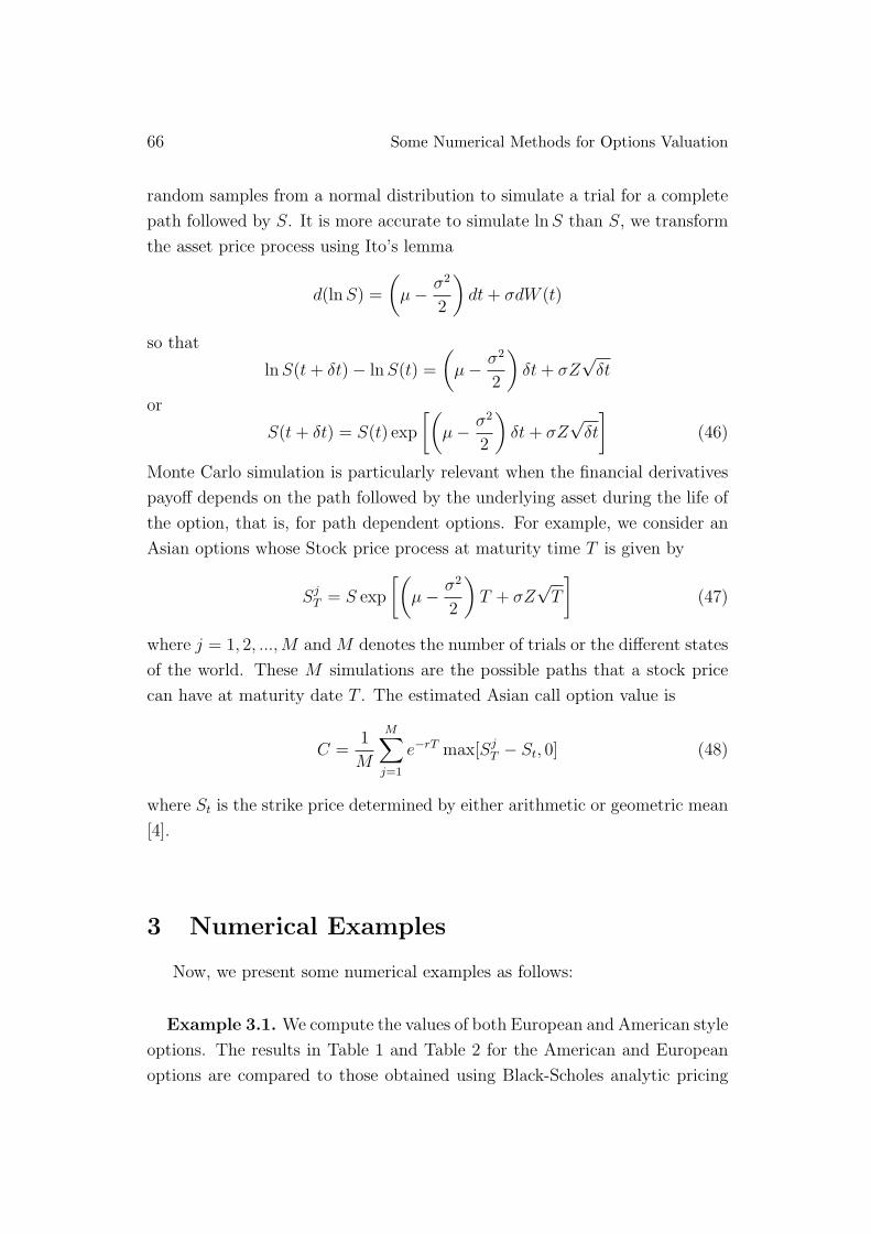
Monte Carlo simulation is particularly relevant when the financial derivatives
payoff depends on the path followed by the underlying asset during the life of
the option, that is, for path dependent options. For example, we consider an
Asian options whose Stock price process at maturity time T is given by
SjT = S exp
[(
µ− σ2
2
)
T + σZ√T
]
(47)
where j = 1, 2, ...,M and M denotes the number of trials or the different states
of the world. These M simulations are the possible paths that a stock price
can have at maturity date T . The estimated Asian call option value is
C =1
M
M∑
j=1
e−rT max[SjT − St, 0] (48)
where St is the strike price determined by either arithmetic or geometric mean
[4].
3 Numerical Examples
Now, we present some numerical examples as follows:
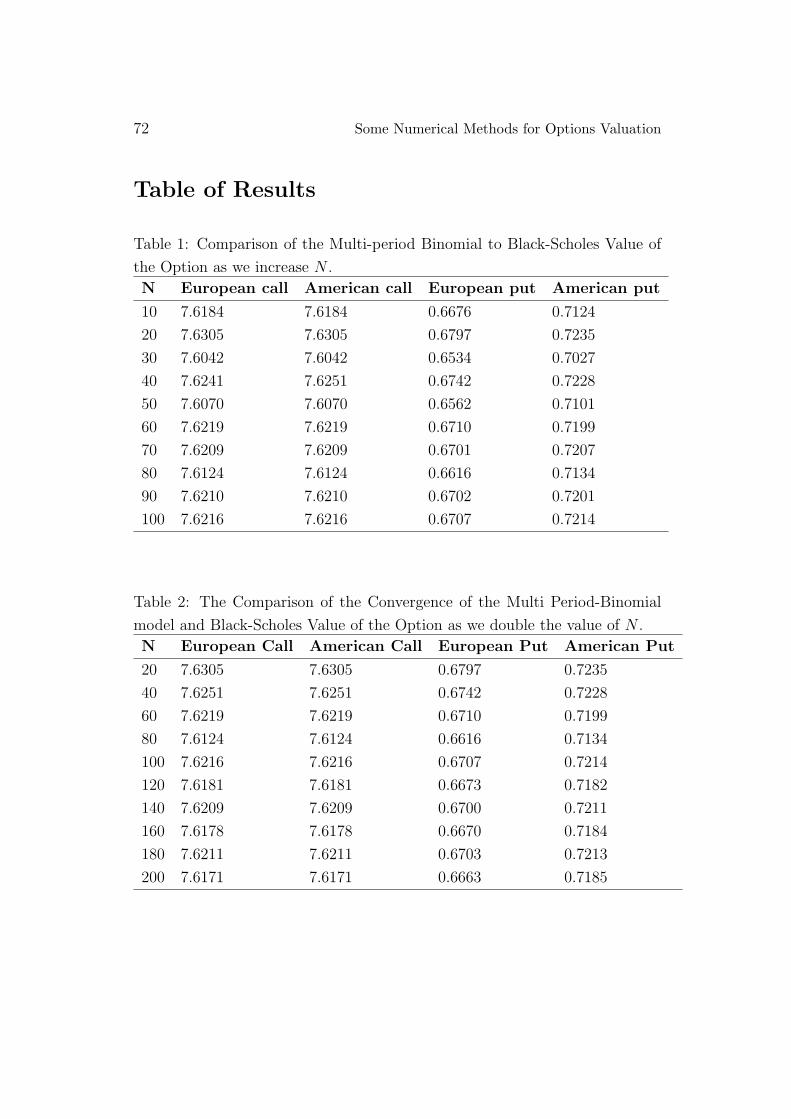
Example 3.1. We compute the values of both European and American style
options. The results in Table 1 and Table 2 for the American and European
options are compared to those obtained using Black-Scholes analytic pricing

C.R. Nwozo and S.E. Fadugba 67
formula. The rate of convergence for multi-period method may be assessed
by repeatedly doubling the number of time steps N . Tables 1 and 2 use the
parameters:
S = 45, K = 40, T = 0.5, r = 0.1, σ = 0.25
in computing the options prices as we increase the number of steps. The Black-
Scholes price for call option and put option are 7.6200 and 0.6692 respectively.
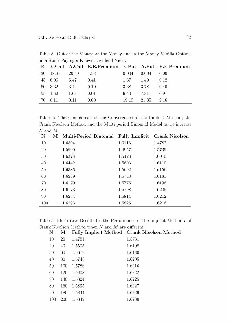
Example 3.2. Consider pricing a vanilla option on a stock paying a known
dividend yield with the following parameters:
S = 50, r = 0.1, T = 0.5, σ = 0.25, τ =1
6, λ = 0.05
The results obtained are shown in the Table 3 below.
Example 3.3. We consider the convergence of the multi-period binomial
model, fully implicit and the Crank Nicolson method with relation to the
Black-Scholes value of the option. We price the European call option on a non
dividend paying stock with the following parameters:
S = 50, K = 60, r = 0.05, σ = 0.2, T = 1
The Black-Scholes price for the call option is 1.6237. The results obtained are
shown in the Tables 4 and 5.
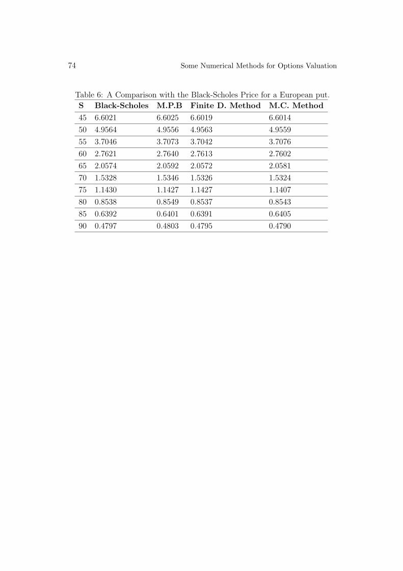
Example 3.4. We consider the performance of the three numerical meth-
ods against the ‘true’ Black-Scholes price for a European put with
K = 50, r = 0.05, σ = 0.25, T = 3
The results obtained are shown in the Table 6 below.
Next, we will now attempt to price an Asian options for which there is no
closed form solution available.
68 Some Numerical Methods for Options Valuation
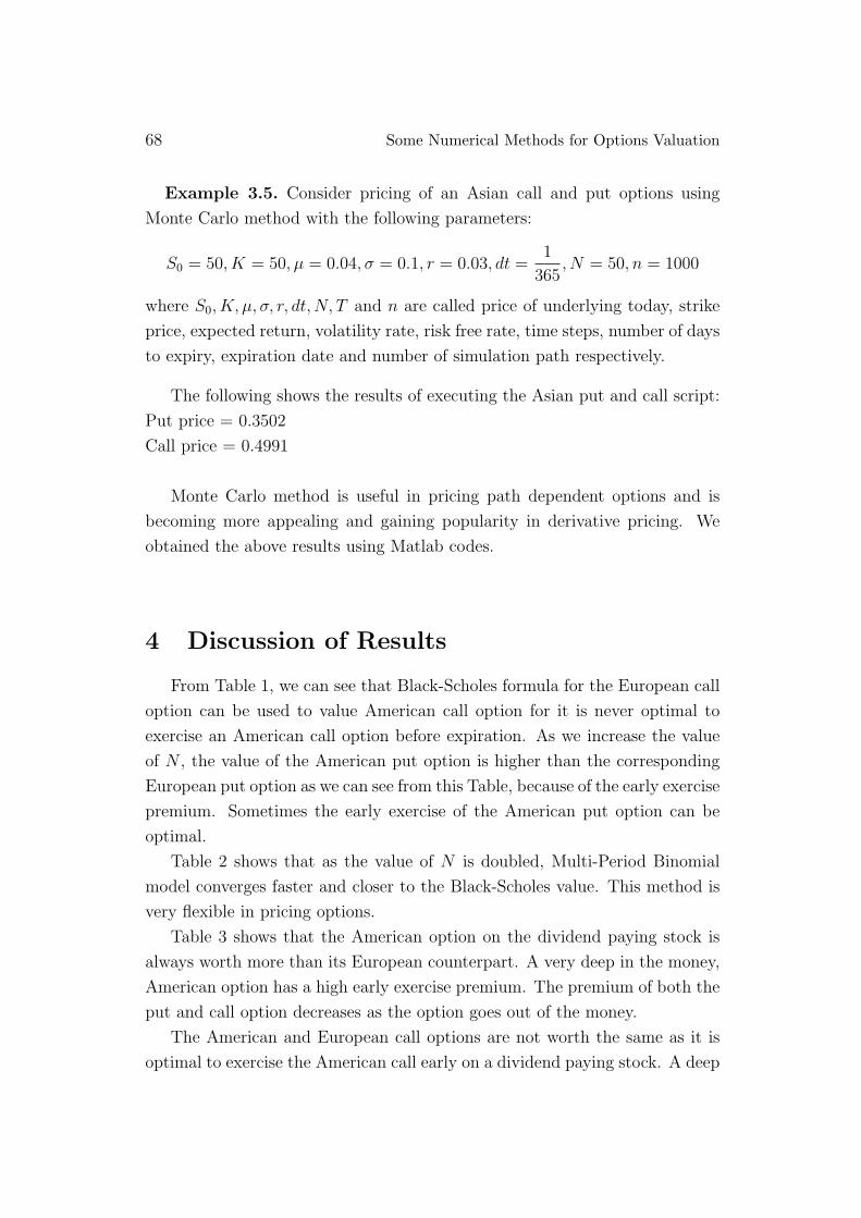
Example 3.5. Consider pricing of an Asian call and put options using
Monte Carlo method with the following parameters:
S0 = 50, K = 50, µ = 0.04, σ = 0.1, r = 0.03, dt =1
365, N = 50, n = 1000
where S0, K, µ, σ, r, dt, N, T and n are called price of underlying today, strike
price, expected return, volatility rate, risk free rate, time steps, number of days
to expiry, expiration date and number of simulation path respectively.
The following shows the results of executing the Asian put and call script:
Put price = 0.3502
Call price = 0.4991
Monte Carlo method is useful in pricing path dependent options and is
becoming more appealing and gaining popularity in derivative pricing. We
obtained the above results using Matlab codes.
4 Discussion of Results
From Table 1, we can see that Black-Scholes formula for the European call
option can be used to value American call option for it is never optimal to
exercise an American call option before expiration. As we increase the value
of N , the value of the American put option is higher than the corresponding
European put option as we can see from this Table, because of the early exercise
premium. Sometimes the early exercise of the American put option can be
optimal.
Table 2 shows that as the value of N is doubled, Multi-Period Binomial
model converges faster and closer to the Black-Scholes value. This method is
very flexible in pricing options.
Table 3 shows that the American option on the dividend paying stock is
always worth more than its European counterpart. A very deep in the money,
American option has a high early exercise premium. The premium of both the
put and call option decreases as the option goes out of the money.
The American and European call options are not worth the same as it is
optimal to exercise the American call early on a dividend paying stock. A deep

C.R. Nwozo and S.E. Fadugba 69
out of the money, American and European call and put options are worth the
same. This is due to the fact that they might not be exercised early as they
are worthless.
Table 4 shows that the Crank Nicolson method in (32) converges faster than
fully implicit method in (31) as N → ∞, δt → 0 and as M → ∞, δS → 0.
The multi-period binomial is closer to the solution for small values of N than
the two finite difference methods.
Table 5 shows that when N and M are different, the finite difference meth-
ods converges faster than when N andM the same. For the implicit and Crank
Nicolson schemes, the number of time steps N initially set at 10 and doubled
with each grid M refinement. We conclude that the finite difference methods,
just as the binomial model are very powerful in pricing of vanilla options. The
Crank Nicolson method has a higher accuracy than the implicit method and
therefore it converges faster. The results obtained highlight that the two finite
difference methods are unconditionally stable.
Table 6 shows the variation of the option price with the underlying price S.
The results demonstrate that the three numerical methods perform well, are
mutually consistent and agree with the Black-Scholes value. However, finite
difference method (F.D.M) is the most accurate and converges faster than
multi period binomial model (M.P.B) and Monte Carlo method (M.C.M).
5 Conclusion
We have at our disposal three numerical methods for options valuation. In
general, each of the three numerical methods has its advantages and disadvan-
tages of use. Binomial models are good for pricing options with early exercise
opportunities and they are relatively easy to implement but can be quite hard
to adapt to more complex situations. Finite difference methods converge faster
and more accurate, they are fairly robust and good for pricing vanilla options
where there is possibilities of early exercise. They can also require sophis-
ticated algorithms for solving large sparse linear systems of equations and
are relatively difficult to code. Finally, Monte Carlo method works very well
for pricing European options, approximates every arbitrary exotic options, it
is flexible in handling varying and even high dimensional financial problems,

70 Some Numerical Methods for Options Valuation
moreover, despite significant progress, early exercise remain problematic for
Monte Carlo method.
Among the methods considered in this work, we conclude that Crank Nicol-
son finite difference method is unconditionally stable, more accurate and con-
verges faster than binomial model and Monte Carlo Method when pricing
vanilla options as shown in Table 4 and Table 6, while Monte carlo simulation
method is good for pricing path dependent options.
When pricing options the important thing is to choose the correct numerical
method from the wide array of methods available.
References
[1] W. Ames, Numerical Methods for Partial Differential Equations, Aca-
demic Press, New York, 1977.
[2] F. Black and M. Scholes, The Pricing of Options and Corporate Liabilities,
Journal of Political Economy, 81(3), (1973), 637-654.
[3] P. Boyle, Options: A Monte Carlo Approach, Journal of Financial Eco-
nomics, 4(3), (1977), 323-338.
[4] P. Boyle , M. Broadie and P. Glasserman, Monte Carlo Methods for Secu-
rity Pricing, Journal of Economic Dynamics and Control, 21(8-9), (1997),
1267-1321.
[5] M. Brennan and E. Schwartz, Finite Difference Methods and Jump Pro-
cesses Arising in the Pricing of Contingent Claims, Journal of Financial
and Quantitative Analysis, 5(4), (1978), 461-474.
[6] J. Cox, S. Ross and M. Rubinstein, Option Pricing: A Simplified Ap-
proach, Journal of Financial Economics, 7, (1979), 229-263.
[7] J. Hull, Options, Futures and other Derivatives, Pearson Education Inc.
Fifth Edition, Prentice Hall, New Jersey, 2003.
[8] R.C. Merton, Theory of Rational Option Pricing, Bell Journal of Eco-
nomics and Management Science, 4(1), (1973), 141-183.
C.R. Nwozo and S.E. Fadugba 71
[9] C. Nwozo, S. Fadugba and T. Babalola, The Comparative Study of Finite
Difference Method and Monte Carlo Method for Pricing European Option,
Mathematical Theory and Modeling, USA, 2(4), (2012), 60-66.
[10] G.D. Smith, Numerical Solution of Partial Differential Equations: Finite
Difference Methods, Clarendon Press, Third Edition, Oxford, 1985.
[11] D. Tavella and C. Randall, Pricing Financial Instruments: The Finite
Difference Method, John Wiley and Sons, New York, 2000.
[12] A. Tveito and R. Winther, Introduction to Partial Differential Equation
Instruments: The Finite Difference Method, John Wiley and Sons, New
York, 1998.
[13] J. Weston, T. Copeland and K. Shastri, Financial Theory and Corporate
Policy, Fourth Edition, New York, Pearson Addison Wesley, 2005.
[14] J. Zhou, Option Pricing and Option Market in China, University of Not-
tingham, 2004.
72 Some Numerical Methods for Options Valuation
Table of Results
Table 1: Comparison of the Multi-period Binomial to Black-Scholes Value of
the Option as we increase N .
N European call American call European put American put
10 7.6184 7.6184 0.6676 0.7124
20 7.6305 7.6305 0.6797 0.7235
30 7.6042 7.6042 0.6534 0.7027
40 7.6241 7.6251 0.6742 0.7228
50 7.6070 7.6070 0.6562 0.7101
60 7.6219 7.6219 0.6710 0.7199
70 7.6209 7.6209 0.6701 0.7207
80 7.6124 7.6124 0.6616 0.7134
90 7.6210 7.6210 0.6702 0.7201
100 7.6216 7.6216 0.6707 0.7214
Table 2: The Comparison of the Convergence of the Multi Period-Binomial
model and Black-Scholes Value of the Option as we double the value of N .
N European Call American Call European Put American Put
20 7.6305 7.6305 0.6797 0.7235
40 7.6251 7.6251 0.6742 0.7228
60 7.6219 7.6219 0.6710 0.7199
80 7.6124 7.6124 0.6616 0.7134
100 7.6216 7.6216 0.6707 0.7214
120 7.6181 7.6181 0.6673 0.7182
140 7.6209 7.6209 0.6700 0.7211
160 7.6178 7.6178 0.6670 0.7184
180 7.6211 7.6211 0.6703 0.7213
200 7.6171 7.6171 0.6663 0.7185
C.R. Nwozo and S.E. Fadugba 73
Table 3: Out of the Money, at the Money and in the Money Vanilla Options
on a Stock Paying a Known Dividend Yield.
K E.Call A.Call E.E.Premium E.Put A.Put E.E.Premium
30 18.97 20.50 1.53 0.004 0.004 0.00
45 6.06 6.47 0.41 1.37 1.49 0.12
50 3.32 3.42 0.10 3.38 3.78 0.40
55 1.62 1.63 0.01 6.40 7.31 0.91
70 0.11 0.11 0.00 19.19 21.35 2.16
Table 4: The Comparison of the Convergence of the Implicit Method, the
Crank Nicolson Method and the Multi-period Binomial Model as we increase
N and M .N = M Multi-Period Binomial Fully Implicit Crank Nicolson
10 1.6804 1.3113 1.4782
20 1.5900 1.4957 1.5739
30 1.6373 1.5423 1.6010
40 1.6442 1.5603 1.6110
50 1.6386 1.5692 1.6156
60 1.6289 1.5743 1.6181
70 1.6179 1.5776 1.6196
80 1.6178 1.5798 1.6205
90 1.6254 1.5814 1.6212
100 1.6293 1.5826 1.6216
Table 5: Illustrative Results for the Performance of the Implicit Method and
Crank Nicolson Method when N and M are different.N M Fully Implicit Method Crank Nicolson Method
10 20 1.4781 1.5731
20 40 1.5505 1.6108
30 60 1.5677 1.6180
40 80 1.5748 1.6205
50 100 1.5786 1.6216
60 120 1.5808 1.6222
70 140 1.5824 1.6225
80 160 1.5835 1.6227
90 180 1.5844 1.6229
100 200 1.5849 1.6230
74 Some Numerical Methods for Options Valuation
Table 6: A Comparison with the Black-Scholes Price for a European put.
S Black-Scholes M.P.B Finite D. Method M.C. Method
45 6.6021 6.6025 6.6019 6.6014
50 4.9564 4.9556 4.9563 4.9559
55 3.7046 3.7073 3.7042 3.7076
60 2.7621 2.7640 2.7613 2.7602
65 2.0574 2.0592 2.0572 2.0581
70 1.5328 1.5346 1.5326 1.5324
75 1.1430 1.1427 1.1427 1.1407
80 0.8538 0.8549 0.8537 0.8543
85 0.6392 0.6401 0.6391 0.6405
90 0.4797 0.4803 0.4795 0.4790