J Nonlinear SciDOI 10.1007/s00332-013-9191-4

Some Joys and Trials of Mathematical Neuroscience

Philip Holmes

Received: 7 August 2013 / Accepted: 30 October 2013© Springer Science+Business Media New York 2013

Abstract I describe the basic components of the nervous system—neurons and theirconnections via chemical synapses and electrical gap junctions—and review themodel for the action potential produced by a single neuron, proposed by Hodgkin andHuxley (HH) over 60 years ago. I then review simplifications of the HH model andextensions that address bursting behavior typical of motoneurons, and describe somemodels of neural circuits found in pattern generators for locomotion. Such circuitscan be studied and modeled in relative isolation from the central nervous system andbrain, but the brain itself (and especially the human cortex) presents a much greaterchallenge due to the huge numbers of neurons and synapses involved. Nonetheless,simple stochastic accumulator models can reproduce both behavioral and electro-physiological data and offer explanations for human behavior in perceptual decisions.In the second part of the paper I introduce these models and describe their relation toan optimal strategy for identifying a signal obscured by noise, thus providing a normagainst which behavior can be assessed and suggesting reasons for suboptimal per-formance. Accumulators describe average activities in brain areas associated with thestimuli and response modes used in the experiments, and they can be derived, albeitnon-rigorously, from simplified HH models of excitatory and inhibitory neural pop-

Communicated by P. Newton.

P. Holmes (B)Department of Mechanical and Aerospace Engineering, Program in Applied and ComputationalMathematics, Princeton University, Princeton, NJ 08544, USAe-mail: pholmes@math.princeton.edu

P. HolmesPrinceton Neuroscience Institute, Princeton University, Princeton, NJ 08544, USA

J Nonlinear Sci

ulations. Finally, I note topics excluded due to space constraints and identify someopen problems.

Keywords Accumulator · Averaging · Central pattern generator · Decision making ·Bifurcation · Drift-diffusion process · Mean field reduction · Optimality ·Phase reduction · Speed-accuracy tradeoff

Mathematics Subject Classification 34Cxx · 34Dxx · 37Cxx · 37N25 · 60H10 ·91E10 · 92C20

1 Introduction

Neuroscience is currently generating much excitement and some hyperbole (a re-cent review of a popular book referred to “neuromania” (McGinn 2013)). This islargely due to recent advances in experimental techniques and associated meth-ods for analysis of “big data.” Striking examples are the CLARITY methodthat allows imaging of entire neural circuits and captures subcellular structuraldetail (Chung et al. 2013), and Connectomics (Seung 2012), which aims to deter-mine neural connectivity and hence function at the cellular level. In announcing theUS Brain Initiative in April 2013, President Obama spoke of “giving scientists thetools they need to get a dynamic picture of the brain in action and better under-stand how we think and how we learn and how we remember” (Insel et al. 2013).Such tools are not solely experimental (Abbott 2008). Computational approachesalready play a substantial rôle in neuroscience (De Schutter 2008, 2009), and theyare becoming more ambitious: the European Blue Brain project (Markram 2006)(http://bluebrain.epfl.ch/) proposes to simulate all the cells and most of the synapsesin an entire brain, thereby hoping to “challenge the foundations of our understandingof intelligence and generate new theories of consciousness.”

In this article I have a more modest goal: to show how mathematical models andtheir analyses are contributing to our understanding of some small parts of brainsand central nervous systems. I will describe how reductions of biophysically basedmodels of single cells and circuits to low-dimensional dynamical systems can re-veal mechanisms that might otherwise remain hidden in massive data analyses andcomputer simulations. In this regard mathematics does not merely enable numericalsimulation and motivate experiments, it provides an analytical complement withoutwhich they can lose direction and lack explanatory power.

Mathematical treatments of the nervous system began in the mid 20th century.An early example is Norbert Wiener’s “Cybernetics,” published in 1948 and basedon work with the Mexican physiologist Arturo Rosenblueth (Wiener 1948). Weinerintroduced ideas from dissipative dynamical systems, symmetry groups, statisticalmechanics, time series analysis, information theory, and feedback control. He alsodiscussed the relationship between digital computers (then in their infancy) and neu-ral circuits, a theme that John von Neumann subsequently addressed in a book pub-lished in the year following his death (von Neumann 1958). While developing oneof the first programmable digital computers (JONIAC, built at the Institute for Ad-vanced Study in Princeton in the late 1940s), von Neumann “tried to imitate some

J Nonlinear Sci

of the known operations of the live brain” (von Neumann 1958, Preface). In devel-oping cybernetics, Wiener drew on von Neumann’s earlier works in analysis, ergodictheory, computation and game theory, as well his own studies of Brownian motion(a.k.a. Wiener processes). Some of these ideas appear in Sect. 4 of the present paper.

These books (Wiener 1948; von Neumann 1958) were directed at the brain andnervous system in toto, although much of the former was based on detailed studiesof heart and leg muscles in animals. The first cellular-level mathematical model of asingle neuron was developed in the early 1950s by the British physiologists Hodgkinand Huxley (1952d). This work, which won them the Nobel Prize in Physiology in1963, grew out of a long series of experiments on the giant axon of the squid Loligoby themselves and others, as noted in Sect. 2 (also see Huxley’s obituary (Mackey andSantillán 2013)). Since their pioneering work, mathematical neuroscience has growninto a subdiscipline, served worldwide by courses long and short (e.g. Kopell et al.2009, Whittington et al. 2009), textbooks (e.g. Wilson 1999, Dayan and Abbott 2001,Keener and Sneyd 2009, Ermentrout and Terman 2010, Gabbiani and Cox 2010), andreview articles (recent examples include Wang 2010, Kopell et al. 2010, McCarthyet al. 2012, Deco et al. 2013). The number of mathematical models must now exceedthe catalogue of brain areas by several orders of magnitude. I can present but fewexamples here, inevitably biased toward my own interests.

Models can be of two broad types: empirical (also called descriptive or phe-nomenological), or mechanistic. The former ignore (possibly unknown) anatomicalstructure and physiology, and seek to reproduce input–output or stimulus–responserelationships of the system under study. Mechanistic models attempt to describestructure and function in some detail, reproducing observed behaviors by appropri-ate choice of model components and parameters and thereby revealing mechanismsresponsible for those behaviors. Models can reside throughout a continuum frommolecular to organismal scales, and many are not easily classifiable, but one commonfeature is nonlinearity. Unlike much of physical science and engineering, biology isinherently nonlinear. For example, the functions describing ion channels opening incells in response to transmembrane voltage increase or characterizing neural firingrate dependence on input current are typically bounded above and below, and oftenmodeled by sigmoids.

The first part of this article covers mechanistic models, beginning in Sect. 2 withthe Hodgkin–Huxley (HH) equations for the generation and propagation of a singleaction potential (AP, or spike); it then discusses dimensional reductions that are easierto analyze and extensions of HH to describe neurons that emit bursts of spikes, andintroduces models for synapses. Section 3 considers small neural circuits found incentral pattern generators for locomotion, and shows how HH models of them can besimplified to phase oscillators. While mathematical methods such as averaging anddimensional reduction via time scale separation are used to simplify coupled sets ofHH equations in these cases, the models are all based on cellular biophysiology.

In Sect. 4 I change scale to introduce empirical models of activity in brain areasthat may contain millions of neurons. Focusing on simple binary decisions in which anoisy stimulus must be identified, I show how a pair of competing nonlinear stochas-tic accumulators can model the integration of noisy evidence toward a threshold, trig-gering a response. Linearizing and considering a limiting case, this model reduces to

J Nonlinear Sci

a scalar drift-diffusion (DD) process, which is in turn a continuum limit of the se-quential probability ratio test (SPRT). The SPRT is known to be optimal in that itrenders decisions of specified accuracy in the shortest possible time. The tractabilityof the DD process allows one to derive an explicit optimal speed-accuracy tradeoff,against which human and animal behavior can be assessed. Behavioral experimentsreveal both approximations to and deviations from optimality, and further analyses ofthe model and data suggest three potential reasons for the latter: avoidance of errors,poor time estimation, and minimization of the cost of cognitive control.

Section 5 sketches computations based on mean-field theory which start with poolsof spiking neurons having distinct “tuning curves” that respond differently to the twostimuli and lead to stochastic accumulator models like those of Sect. 4. While thisis neither rigorous nor as complete as the reduction methods of Sect. 3, it providesfurther support for such models by connecting them to simplified neuron models ofHH type. It also suggests a fourth, physiological reason for suboptimality, namely,nonlinear dynamics. Section 6 contains a brief discussion, provides references someof the many topics omitted due to space limitations, and notes some open problems.

2 The Components: Neurons, Synapses and the Hodgkin–Huxley Equations

The basic components of the nervous system are neurons: electrically active cellsthat can generate and propagate signals over distance. These signals are action po-tentials (APs, or spikes): voltage fluctuations of O(100) mV, each lasting 1–5 msec,across the cell membrane. Structurally, neurons come in many shapes and sizes, butall share the basic features of a soma or cell body, dendrites: multiply branchingextensions that receive signals from other neurons, and an axon, a cable-like exten-sion that may also be branched, along which APs propagate to other neurons.1 Theconnections between axons and dendrites are called synapses, and they may be elec-trical, communicating voltage differences, or chemical, releasing neurotransmittersupon the arrival of an AP from the presynaptic cell. Functionally, neurons are eitherexcitatory or inhibitory, tending to increase or depress the transmembrane voltageof postsynaptic cells to which they connect. In this section we describe models forsingle neurons and for synapses.

2.1 The Hodgkin–Huxley Equations

As noted above, following years of beautiful and painstaking experiments reportedin an impressive series of papers (Hodgkin et al. 1949, 1952; Hodgkin and Hux-ley 1952b,a,c), Hodgkin and Huxley created the first mathematical model for theAP (Hodgkin and Huxley 1952d). This work gained them a Nobel prize in 1963,along with J.C. Eccles (for work on synapses and discovery of excitatory and in-hibitory postsynaptic potentials: see Sect. 2.5). They used the giant axon of a squid,part of the animal’s escape reflex system. The cell’s size allowed them to thread asilver wire through it, equalizing voltages along the axon, thus removing spatial vari-ations and allowing them to describe its dynamics in terms of nonlinear ordinary

1Biologists refer to dendrites and axons as processes: confusing terminology for a mathematician!

J Nonlinear Sci

Fig. 1 Equivalent circuit for thegiant axon of squid,from Hodgkin and Huxley(1952d, Fig. 1). Leakconductance is constant, butsodium and potassiumconductances vary, indicated byvariable resistors. Batteriesrepresent reversal potentials,transmembrane capacitance isCm µF/cm2 and applied currentis I µA/cm2

differential equations (ODEs):

Cm

dv

dt= −gKn4(v − vK) − gNam

3h(v − vNa) − gL(v − vL) + I, (1a)

dm

dt= αm(v)(1 − m) − βm(v)m, (1b)

dn

dt= αn(v)(1 − n) − βn(v)n, (1c)

dh

dt= αh(v)(1 − h) − βh(v)h. (1d)

(A term ∂2v

∂x2 was subsequently added to (1a) to model propagation of the AP alongthe axon (Hodgkin and Huxley 1952d), creating a reaction–diffusion equation.) I nowbriefly describe the electro-chemical mechanisms encoded in the ODEs (1a–1d);for further details and historical notes, see Keener and Sneyd (2009, Sect. 5.1),and Hodgkin and Huxley (1952d).

Before starting it is important to know that ionic transport across cell membranesoccurs through ion-specific channels and pores. It is driven passively by concentra-tion and potential differences and by active pumps that exchange sodium for potas-sium and remove calcium from the cell. The Nernst–Planck equation, from bio-physics, relates transmembrane flux, concentration and potential differences for eachionic species, and allows one to compute equilibrium conditions consistent with zeroflux (Keener and Sneyd 2009, Sect. 2.6). At this resting potential, sodium concen-trations are higher outside the cell than inside, while potassium concentrations arehigher inside it.

Hodgkin and Huxley had noted that during a spike the initial inward current wasfollowed by an outward current. They hypothesized that the former was due to sodiumions (Na+) flowing in from their higher extracellular concentration, and that the out-ward current was due to potassium ions (K+) leaving the cell. They also included apassive leak current, due primarily to chloride ions (Cl−). These three currents ap-pear in (1a) as gNam

3h(v−vNa), gKn4(v−vK), and gL(v−vL) µA/cm2 respectively,along with an externally applied current I , corresponding to Kirchhoff’s law whichdescribes the rate of change of transmembrane voltage v in the circuit of Fig. 1. The

J Nonlinear Sci

barred parameters in the sodium and potassium conductances denote constant valuesthat multiply time-dependent functions of n(t),m(t) and h(t) to form “dynamical”conductances gKn4 and gNam

3h. Voltage dependencies of the ion channels are alsocharacterized by the Nernst reversal potentials vK = −12 mV, vNa = 115 mV andvL = 10.6 mV; as the name suggests, the currents change direction as v crosses thesevalues.

The rôle of each ionic species was revealed by experiments in which all but oneactive species were removed and the transmembrane voltage held constant and thenstepped from one value to another, while the current I (t) required to maintain thatvoltage was recorded. This voltage clamp method determined each ionic conduc-tance as a function of voltage. Moreover, by examining transient responses followingsteps of given sizes, Hodgkin and Huxley could fit sigmoids to the six functionsαm(v), . . . βh(v) across the relevant voltage range. (Note that (1b–1d) are linear forfixed v.) They postulated a single gating variable n(t) ∈ [0,1] to describe potassiumactivation and noted that while conductance dropped sharply from higher levels fol-lowing a downward step in v, it rose gently from zero after a step increase. This ledto the fourth power in the potassium conductance gKn4 (cf. Hodgkin and Huxley1952d, Figs. 2 and 3). Sodium dynamics proved more complicated, involving a rapidincrease in conductance followed by slower decrease (Hodgkin and Huxley 1952d,Fig. 6), a non-monotonic response that required two variables m(t), h(t) ∈ [0,1] todescribe activation and deactivation, producing the m3h term in gNam

3h.The resulting forms of the α and β functions are

αm(v) = 0.125 − v

exp( 25−v10 ) − 1

, βm(v) = 4 exp

(−v

18

), (2)

αh(v) = 0.07 exp

(−v

20

), βh(v) = 1

exp( 30−v10 ) + 1

, (3)

αn(v) = 0.0110 − v

exp( 10−v10 ) − 1

, βn(v) = 0.125 exp

(−v

80

), (4)

and the conductances are gNa = 120, gK = 36, and gL = 0.3 mSiemens/cm2. Toemphasize the equilibrium potential n∞(v) at which n remains constant, and the timescale τn(v), the gating equations may be rewritten as follows:

dn

dt= n∞(v) − n

τn(v), where

n∞(v) = αn(v)

αn(v) + βn(v), τn(v) = 1

αn(v) + βn(v), (5)

with analogous expressions for m and h. See Hodgkin and Huxley (1952d, Figs. 4–5,7–8 and 9–10) for graphs of αn(v),βn(v), n∞(v), etc.

Figure 2 shows time courses of voltage and gating variables during a typical AP,obtained by numerical solution of (1a)–(1d). Note the four phases:

(1) rapid increase in v and m as sodium conductance rises towards the sodium Nernstpotential in a brief depolarized AP.

J Nonlinear Sci

Fig. 2 (a) Time courses ofmembrane voltage (a) andgating variables (b) during anaction potential and thesubsequent refractory andrecovery periods: m solid,n dash-dotted and h dashed.Voltage scale has been shifted sothat resting potential is at 0 mV.Note the differing timescalesand approximate anticorrelationof n(t) and h(t)

(2) At higher voltages h decreases, lowering sodium conductance, and n increases,increasing potassium conductance and driving v down towards the potassiumpotential.

(3) During the ensuing refractory period m falls quickly to its resting value, but n

stays high and h remains low because their equations have longer time constants,thus holding v down (hyperpolarized) and preventing APs.

(4) As n and h return to values that allow an AP, the cell enters its recovery phase.

The variables m,n and h can be interpreted as probabilities that gates in the cor-responding ionic channels are open, and the exponents in the conductances as thenumbers of gates that must be open. It is now known that potassium channels con-tain tetrameric structures that must cooperate for ions to flow, in agreement with theempirical n4 fit.

J Nonlinear Sci

Fig. 3 Phase planes of thereduced HH equations(7a)–(7b), showing nullclinesv = 0, n = 0 (bold) for I = 0 (a)and I = 15 (b). Orbits flow tothe left above v = 0 and to theright below it; diamonds at endsof orbit segments indicate flowdirection. Approximatelyhorizontal componentscorrespond to fast flows andsolutions move slowly near theslow manifold v = 0

2.2 Two-Dimensional Reductions of HH

I now introduce two simplifications of the Hodgkin–Huxley equations, a reductionof HH due to Krinsky and Kokoz (1973) and, independently, Rinzel (1985), and theFitzHugh-Nagumo (FN) equations (FitzHugh 1961; Nagumo et al. 1962), (Wilson1999, Chaps. 8–9). Examining the behavior of the HH state variables, we see thatm(t) changes relatively rapidly because its timescale τm = 1/(αm + βm) � τn, τh inthe relevant voltage range (cf. (2–5) and Fig. 2). We may therefore assume that it isalmost always equilibrated so that m ≈ 0, implying that

m(t) ≈ m∞(v) = αm(v)

αm(v) + βm(v), (6)

cf. (5). Moreover, as Fig. 2(b) shows, n(t) and h(t) are approximately anti-correlatedin that throughout the AP and recovery phase their sum remains almost constant:h + n ≈ a. Thus m and h may be replaced by m∞(v) and a − n and dropped as statevariables, reducing the system to

Cm

dv

dt= −gKn4(v − vK) − gNam∞(v)3(a − n)(v − vNa) − gL(v − vL) + I, (7a)

τn(v)dn

dt= n∞(v) − v. (7b)

This reduction to a planar system can be made rigorous by use of geometric singularperturbation methods (Jones 1994).

Planar system methods (Hirsch et al. 2004) reveal the phase portrait of (7a)–(7b).The n = 0 nullcline, on which solutions move vertically in Fig. 3, can be writtenexplicitly, but the v = 0 nullcline, for horizontal motion, demands solution of a quar-tic polynomial, which can be done numerically to yield the phase portrait of Fig. 3.Fixed points lie at the intersections of these nullclines. The left-hand plot, for I = 0,features a sink near v = 0 along with a saddle and a source. In the right-hand plot,

J Nonlinear Sci

Fig. 4 Phase planes of theFizHugh–Nagumo equations(8a)–(8b), showing nullclinesand indicating fast and slowflows for τv = 0.1, τr = 1.25,and I = 0 (left) and I = 1.5(right). At left, all orbitsapproach a sink; at right a limitcycle encircles a source. Orbitsshown as in Fig. 3

for I = 15, a limit cycle has appeared. Figure 3 displays the spiking threshold vthat a local minimum of the v = 0 nullcline. When the leftmost fixed point lies to theleft of vth it is stable, as for I = 0. In this excitable state spikes can occur due toperturbations that push v past vth, but absent further perturbations the state returnsto the sink. When the fixed point moves to the right of vth (I = 15) it loses stabilityand solutions repeatedly cross threshold, yielding periodic spiking in the manner ofa relaxation oscillator (Guckenheimer and Holmes 1983, Sect. 2.1).

Here, to illustrate the rich dynamics that a planar system with nonlinear nullclinescan exhibit, we have chosen I values for which (7a)–(7b) has three fixed points; forothers, it has only one (as do the original H–H equations) (Rinzel 1985).

The FN equations preserve this qualitative structure, replacing the complicatedsigmoids of (2–4) by cubic and linear functions:

v = 1

τv

(v − v3

3− r + I

), (8a)

r = 1

τr

(−r + 1.25v + 1.5), (8b)

Wilson (1999, Sect. 8.3). Timescales are normally chosen so that τv � τr = O(1) topreserve the relaxation oscillation with fast rise and fall in v, but the relative durationsof the depolarized and hyperpolarized episodes are approximately equal, unlike theHH dynamics of Fig. 2. The reason for this becomes clear when we examine thenullclines shown in Fig. 4.

First note that the basic behavior of the reduced HH equations (7a)–(7b) is pre-served: for low I (on the left), there is a stable sink, while for higher I (on the right),there is a stable limit cycle. However, unlike Fig. 3, the cubic v = 0 nullcline is sym-metric about v = 0, so that the slow orbit segments are similar in duration. Moreover,since the slope of the r = 0 nullcline (1.25) exceeds the maximum slope of the v = 0nullcline (1), (8a)–(8b) has a single fixed point for all I . It can be shown that thisloses stability in a supercritical Hopf bifurcation (Guckenheimer and Holmes 1983,Sect. 3.4) as I increases, creating the limit cycle, and that the limit cycle vanishes in asecond Hopf bifurcation at a higher I , where the fixed point restabilizes, correspond-ing to persistent depolarization of the neuron. This bifurcation sequence also occursfor the full HH equations, but in that case the first Hopf bifurcation is subcritical, in

J Nonlinear Sci

Fig. 5 Periodic spiking in aleaky IF model for vss > vth,including a refractory period.Trajectory of v(t) withoutthreshold shown dashed andmarked vss (in red)(Color figure online)

which an unstable limit cycle converges on the stable hyperpolarized fixed point. Theunstable cycle appears in a saddle-node bifurcation of periodic orbits (Guckenheimerand Holmes 1983, Sect. 3.5), along with a stable limit cycle at a slightly lower I . TheFN simplification loses both quantitative and fine qualitative detail, but is nonethelesspopular among applied mathematicians due to its analytical tractability.

2.3 Integrate-and-Fire Models

Integrate-and-fire (IF) models effect further reduction to a single ODE by replac-ing the spike dynamics with a stereotypic AP description inserted when v exceedsa threshold vth, followed by reset to a resting potential vr , possibly after a fixed re-fractory period. The model was first introduced in 1907 in studying the sciatic nerveof leg muscles in frogs (Lapicque 1907; Brunel and van Rossum 2007), but furtherstudies came decades later (Stein 1965; Knight 1972a,b). The linear IF model retainsonly the leak and applied currents of (1a) and is written

Cv = −gL(v − vL) + I, for v ∈ [vr , vth). (9)

A delta function δ(t − tk) is inserted and voltage reset if v reaches vth at t = tk ,making (9) a hybrid dynamical system (Back et al. 1993; Guckenheimer and Johnson1995). Without resets, all solutions would approach the sink at vss = vL + I/gL asthey do for vss ≤ vth, but if vss > vth repetitive spiking occurs as shown in Fig. 5.

The decelerating subthreshold voltage profile of the linear IF model differs fromthe acceleration characteristic of more realistic models (cf. Fig. 2(a)). This can berepaired by using nonlinear functions, common choices being quadratic (Ermen-trout and Kopell 1986; Latham et al. 2000; Latham and Brunel 2003) or exponen-tial (Foucaud-Trocme et al. 2003; Foucaud-Trocme and Brunel 2005). The reset uponreaching threshold prevents orbits escaping to infinity in finite time. See Izhikevich(2004) for comparisons and Burkitt (2006a,b) for model reviews.

Interspike intervals and hence firing rates are easily computed for scalar IF models,but it is difficult to obtain explicit results for all but the simplest multi-unit circuitsbecause one must compute threshold arrival times for every cell and paste togetherthe intervening orbit segments to obtain the flow map. Nonetheless, IF models arein wide use for large-scale numerical simulations of cortical circuits; an exampleappears below in Sect. 5.

J Nonlinear Sci

Fig. 6 Left: A branch ofequilibria (red) for the “frozenc” system containing twosaddle-nodes (SN) and a Hopfbifurcation (H). The v = 0 andc = 0 nullclines and a typicalbursting orbit are projected ontothe (c, v) plane. Right: Thevoltage time history exhibitingperiodic bursts. Adaptedfrom Ghigliazza and Holmes(2004b, Fig. 11)(Color figure online)

2.4 A Model for Bursting Neurons

As well as reducing them, one can augment the HH equations by adding ionic species.Incorporating slow processes such as calcium (Ca++) release introduces long timescales that can interact with the medium and short timescales of periodic APs toproduce bursts of spikes followed by refractory periods. This is characteristic of mo-toneurons, and more generally of cells involved in generating rhythmic activity (Chayand Keizer 1983; Sherman et al. 1988). Let c(t) denote a slow gating variable gov-erned by

τc(v)c = ε(c∞(v) − c

), ε � 1, (10)

and for simplicity suppose that the medium scale ionic dynamics has been reducedto a single variable n, as in (7a)–(7b). The voltage equation analogous to (7a) nowcontains an ionic current depending on c, but since c = O(ε), we may appeal to per-turbation methods (Holmes 2013) and regard c as a “frozen” parameter. Changes inc can cause bifurcations in the two-dimensional (v,n) system that lead from quies-cence (a stable fixed point), to periodic spiking, as in Fig. 3, and the slow dynamicsof (10) can drive the full system periodically between these states.

Figure 6 shows an example from Ghigliazza and Holmes (2004b). For small c

the (v,n) system has a source surrounded by a stable limit cycle, and for high c

a single sink, which continues to the lower saddle-node bifurcation point. The up-per saddle node creates the source and a saddle point. Below the c = 0 nullcline,c decreases, moving the state along the lower, stable branch of equilibria duringthe refractory period. At the lower saddle node, the state jumps to the limit cycle,which lies above c = 0, so that c now increases. However, before reaching the uppersaddle-node the limit cycle collides with the saddle and vanishes in a homoclinic loopbifurcation (Guckenheimer and Holmes 1983, Sect. 6.1).

More on bursting mechanisms and their classification via the fast subsystem’s bi-furcations as the slow c variable drifts back and forth can be found in Wilson (1999,Chap. 10) and Keener and Sneyd (2009, Chap. 9).

J Nonlinear Sci

2.5 Neural Connectivity: Synapses and Gap Junctions

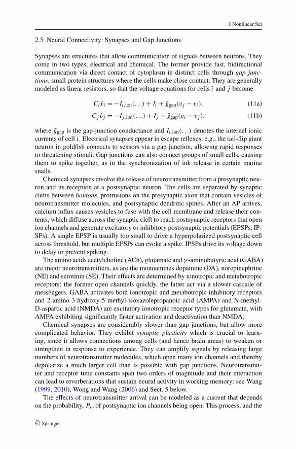
Synapses are structures that allow communication of signals between neurons. Theycome in two types, electrical and chemical. The former provide fast, bidirectionalcommunication via direct contact of cytoplasm in distinct cells through gap junc-tions, small protein structures where the cells make close contact. They are generallymodeled as linear resistors, so that the voltage equations for cells i and j become

Civi = −Ii,ion(. . .) + Ii + ggap(vj − vi), (11a)

Cj vj = −Ij,ion(. . .) + Ij + ggap(vi − vj ), (11b)

where ggap is the gap-junction conductance and Ii,ion(. . .) denotes the internal ioniccurrents of cell i. Electrical synapses appear in escape reflexes: e.g., the tail-flip giantneuron in goldfish connects to sensors via a gap junction, allowing rapid responsesto threatening stimuli. Gap junctions can also connect groups of small cells, causingthem to spike together, as in the synchronization of ink release in certain marinesnails.

Chemical synapses involve the release of neurotransmitter from a presynaptic neu-ron and its reception at a postsynaptic neuron. The cells are separated by synapticclefts between boutons, protrusions on the presynaptic axon that contain vesicles ofneurotransmitter molecules, and postsynaptic dendritic spines. After an AP arrives,calcium influx causes vesicles to fuse with the cell membrane and release their con-tents, which diffuse across the synaptic cleft to reach postsynaptic receptors that openion channels and generate excitatory or inhibitory postsynaptic potentials (EPSPs, IP-SPs). A single EPSP is usually too small to drive a hyperpolarized postsynaptic cellacross threshold, but multiple EPSPs can evoke a spike. IPSPs drive its voltage downto delay or prevent spiking.

The amino acids acetylcholine (ACh), glutamate and γ -aminobutyric acid (GABA)are major neurotransmitters, as are the monoamines dopamine (DA), norepinephrine(NE) and serotinin (SE). Their effects are determined by ionotropic and metabotropicreceptors; the former open channels quickly, the latter act via a slower cascade ofmessengers. GABA activates both ionotropic and metabotropic inhibitory receptorsand 2-amino-3-hydroxy-5-methyl-isoxazolepropanoic acid (AMPA) and N-methyl-D-aspartic acid (NMDA) are excitatory ionotropic receptor types for glutamate, withAMPA exhibiting significantly faster activation and deactivation than NMDA.

Chemical synapses are considerably slower than gap junctions, but allow morecomplicated behavior. They exhibit synaptic plasticity which is crucial to learn-ing, since it allows connections among cells (and hence brain areas) to weaken orstrengthen in response to experience. They can amplify signals by releasing largenumbers of neurotransmitter molecules, which open many ion channels and therebydepolarize a much larger cell than is possible with gap junctions. Neurotransmit-ter and receptor time constants span two orders of magnitude and their interactioncan lead to reverberations that sustain neural activity in working memory: see Wang(1999, 2010), Wong and Wang (2006) and Sect. 5 below.

The effects of neurotransmitter arrival can be modeled as a current that dependson the probability, Ps , of postsynaptic ion channels being open. This process, and the

J Nonlinear Sci

closure of channels as the transmitter unbinds from receptors, can be modeled likethe gating variables in the HH equations:

dPs

dt= αs(1 − Ps) − βsPs, (12)

where αs and βs determine the rates at which channels open and close, effectively en-coding the neurotransmitter time scales: see Destexhe et al. (1999, p. 15) and Dayanand Abbott (2001, p. 180). Opening is typically faster than closure, so αs � βs, andβs is often assumed constant, but αs depends on neurotransmitter concentration in thesynaptic cleft, and thus on the presynaptic voltage vi . Again, a sigmoid provides anacceptable model:

αs(vi) = αsCNT,max

1 + exp[−kpre(vi − vpresyn)]

, (13)

(Destexhe et al. 1999; Dayan and Abbott 2001), where CNT,max represents the max-imal neurotransmitter concentration, v

presyn sets the voltage at which vesicles begin to

open, kpre sets the “sharpness” of the switch, and the scale factor αs allows one tolump the effects of all the synapses between the two cells.

As for the internal ionic currents in the HH model, the postsynaptic current in cellj due to an AP in cell i involves a reversal potential, vpost

syn , and is scaled by a maximalconductance, gsyn, so that the voltage equation for the postsynaptic cell is

Cvj = −Ij,ion(. . .) + Ij − gsynPs(vj − v

postsyn

). (14)

Equation (14) and the analogous voltage equations for all presynaptic cells, with theirassociated full or reduced gating equations, are solved together with (12). See Ghigli-azza and Holmes (2004a) for examples.

This model can be simplified by noting that the rapid rise and fall of the AP vi ,acting via (13), makes αs(vi) behave like a rectangular pulse with duration of theAP and height αsCNT,max. Equation (12) may then be solved explicitly during andfollowing the AP and the resulting exponentials matched to produce a piecewise-smooth rising and falling pulse. Alternatively, this may be approximated as a sum oftwo exponentials or as an “alpha” function:

Ps(t) = Pmaxt

τsexp

(1 − t

τs

), t ≥ 0, (15)

which starts at zero, rises to a peak Pmax at t = τs, and then decays back to zerowith time constant τs. For further discussions of synaptic mechanisms, see Dayanand Abbott (2001), Keener and Sneyd (2009, Chap. 8) and Johnston and Wu (1997,Chaps. 11–15).

As noted in Sect. 2.1, Hodgkin and Huxley modeled the propagation of APs alongan axon by adding a diffusive spatial term to (1a) (Hodgkin and Huxley 1952d). Morecomplex geometries including branching dendrites and axons are often representedby multiple compartments (sometimes in the hundreds). This leads to large sets ofODEs for each cell, but allows one to capture subtle effects that influence intercellularcommunication. Not only do dendrite sizes affect their conductances (Rall 1959) and

J Nonlinear Sci

transmission delays occur in dendritic trees, but EPSPs arriving at nearby synapsesinteract to produce less excitation than their sum predicts (Rall et al. 1967). Nonlinearinteractions due to shunting inhibition that changes membrane conductance can alsoreduce excitatory currents (Rall 1964). See London and Häusser (2005) for reviewsof such “dendritic computations.”

3 Central Pattern Generators and Phase Reduction

Central pattern generators (CPGs) are networks in the spinal cords of vertebratesand invertebrate thoracic ganglia, capable of generating muscular activity in the ab-sence of sensory feedback (Cohen et al. 1988; Getting 1988; Pearson 2000; Marder2000; Ijspeert 2008), cf (Wilson 1999, Chaps. 12–13). CPGs drive many rhythmic ac-tions, including locomotion, scratching, whisking (e.g. in rats), moulting (in insects),chewing and digestion. The stomato-gastric ganglion in lobster is perhaps the best-understood example (Marder and Bucher 2007). Experiments are typically done inisolated in vitro preparations, with sensory and higher brain inputs removed (Cohenet al. 1988; Grillner 1999), but it is increasingly acknowledged that an integrativeapproach, including muscle and body-limb dynamics, environmental reaction forcesand proprioceptive feedback, is needed to fully understand their function (Chiel andBeer 1997; Holmes et al. 2006; Tytell et al. 2011). Indeed, without reaction forces,animals would go nowhere! CPGs nonetheless provide examples of neural networkscapable of generating interesting behaviors, but small enough to allow the study ofdetailed biophysically based models.

After introducing a phase reduction method that is particularly useful for suchsystems and applies to any ODE with a hyperbolic limit cycle and showing how itleads to systems of coupled phase oscillators via averaging theory, I describe a modelof an insect CPG. For an early review of CPG models that use phase reduction andaveraging, see Kopell (1988).

3.1 Phase Reduction and Phase Response Curves

Phase reduction was originally developed by Malkin (1949, 1956), and indepen-dently, with biological applications in mind, by Winfree (2001). For extensive treat-ments, see Hoppensteadt and Izhikevich (1997, Chap. 9) and Ermentrout and Terman(2010, Chap. 8). Consider a system

x = f(x) + εg(x, . . .); x ∈ Rn, 0 ≤ ε � 1, n ≥ 2, (16)

where g(x, . . .) represents external inputs (e.g. (16) might be an ODE of HH type(1a)–(1d)) or a busting neuron model (Sect. 2.4). Suppose that (16) possesses a stablehyperbolic limit cycle Γ0 of period T0 for ε = 0, and let x0(t) denote a solution ly-ing in Γ0. Invariant manifold theory (Hirsch et al. 1977; Guckenheimer and Holmes1983) guarantees that, in a neighborhood U of Γ0, the state space splits into a phasevariable ϕ ∈ [0,2π) along the closed curve Γ0 and a smooth foliation of transverseisochrons (Guckenheimer 1975). Each isochron is an (n − 1)-dimensional manifoldMϕ with the property that any two solutions starting on the same leaf Mϕi

are mapped

J Nonlinear Sci

Fig. 7 The direct method forcomputing the PRC, showingthe geometry of isochrons, theeffect of the perturbation at x∗that results in a jump to a newisochron, recovery to the limitcycle, and the resulting phaseshift. Adapted from Brown et al.(2004)

by the flow to another leaf Mϕjand hence approach Γ0 with equal asymptotic phases

as t → ∞: see Fig. 7. For points x ∈ U , phase is therefore defined by a smooth func-tion ϕ(x) and the leaves Mϕ ⊂ U are labeled by the inverse function x(ϕ). Moreover,this structure persists for small ε > 0, so Γ0 perturbs to a nearby limit cycle Γε .

The phase coordinate ϕ(x) is chosen so that progress around the limit cycle occursat constant speed when ε = 0:

ϕ(x(t)

)∣∣x∈Γ0

= ∂ϕ(x(t))

∂x· f

(x(t)

)∣∣∣∣x∈Γ0

= 2π

T0

def= ω0. (17)

Applying the chain rule, using (16) and (17), we obtain the scalar phase equation:

ϕ = ∂ϕ(x)

∂x· x = ω0 + ε

∂ϕ

∂x· g

(x0(ϕ), . . .

)∣∣Γ0(ϕ)

+O(ε2). (18)

The assumption that coupling and external influences are weak (ε � 1) allows ap-proximation of their effects by evaluating g(x, . . .) along Γ0.

For spiking-neuron models in which inputs enter only via the voltage equation

(e.g., (1a)–(1d)), the only nonzero component in the vector ∂ϕ∂x is ∂ϕ

∂V= ∂ϕ

∂x · ∂x∂V

def=z(ϕ). This phase response curve (PRC) describes how an impulsive perturbation ad-vances or retards the next spike as a function of the phase during the cycle at whichit acts. PRCs may be calculated using a finite-difference approximation to the deriva-tive:

z(ϕ) = ∂ϕ

∂V= lim

V →0

[ϕ(x∗ + ( V,0)T) − ϕ(x∗)

V

], (19)

where the numerator ϕ = [ϕ(x∗+( V,0)T)−ϕ(x∗)] describes the change in phasedue to the delta function perturbation V → V + V at x∗ ∈ Γ0: see Fig. 7. PRCs mayalso be found from adjoint equations (Ermentrout and Terman 2010, Chap. 8).

3.2 Weak Coupling, Averaging and Half-Center Oscillators

A common structure appearing in GPG models is the half-center oscillator: a pair ofunits, often identical and hence bilaterally (or reflection-) symmetric and sometimes

J Nonlinear Sci

each containing several neurons, connected via mutual inhibition to produce an alter-nating rhythm (Ermentrout and Terman 2010, Sect. 9.6). See Hill et al. (2001), Daun-Gruhn et al. (2009), Doloc-Mihu and Calabrese (2011) and Wilson (1999, Sect. 13.1)for examples. Phase reduction provides a simple expression of this architectural sub-unit, which can be written as a system on the torus:

ϕ1 = ω0 + ε[δ1 + z1(ϕ1)h1(ϕ1, ϕ2)

] def= ω0 + εH1(ϕ1, ϕ2), (20a)

ϕ2 = ω0 + ε[δ2 + z2(ϕ2)h2(ϕ2, ϕ1)

] def= ω0 + εH2(ϕ2, ϕ1). (20b)

Here small frequency differences εδj are allowed and the O(ε2) terms neglected.Transformation to slow phases ψi = ϕi − ω0t removes the common frequency ω0and puts (20a)–(20b) in a form to which the averaging theorem for periodically forcedODEs can be applied (Guckenheimer and Holmes 1983, Sect. 4.1–2):

ψ1 = εH1(ψ1 + ω0t,ψ2 + ω0t), (21a)

ψ2 = εH2(ψ2 + ω0t,ψ1 + ω0t). (21b)

Recalling that the common period of the uncoupled oscillators is T0, the averagesof the terms on the RHS of (21a)–(21b) are

Hi(ψi,ψj ) = 1

T0

∫ T0

0Hi(ψi + ω0t,ψj + ω0t)dt. (22)

Changing variables by setting τ = ψj + ω0t , so that dt = dτω0

= T0 dτ2π

, and using thefact that the Hi are 2π -periodic, the integral of (22) becomes

Hi(ψi,ψj ) = 1

2π

∫ 2π

0Hi(ψi − ψj + τ, τ )dτ

def= Hi(ψi − ψj); (23)

hence the averaged system (up to O(ε2)) is

ψ1 = εH1(ψ1 − ψ2), ψ2 = εH2(ψ2 − ψ1). (24)

The functions Hi(ψi − ψj) are 2π -periodic and depend only on phase differenceθ = ψ1 − ψ2. Equations (24) may therefore be subtracted to yield

θ = ε[H1(θ) − H2(−θ)

] def= εG(θ). (25)

Phase reduction and averaging have simplified a system with at least two voltagevariables, associated gating variables, and possibly additional synaptic variables, to aflow on the circle.

For mutually symmetric coupling between identical units, h2(ϕ2, ϕ1) = h1(ϕ1, ϕ2)

in (20a)–(20b). Integration preserves this symmetry under permutation of ϕ1 and ϕ2,

so that the averaged functions satisfy H2(−θ) = H1(θ)def= H(θ). In this case, since H

is 2π -periodic, G(π) = H(π) − H(−π) = H(π) − H(π) = 0 and G(0) = H(0) −

J Nonlinear Sci

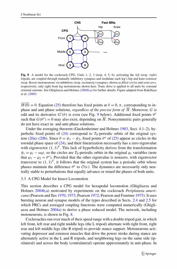
Fig. 8 A model for the cockroach CPG. Units 1, 2, 3 (resp. 4, 5, 6), activating the left (resp. right)tripods, are coupled through mutually inhibitory synapses and modulate each leg’s hip and knee extensor(resp. flexor) motoneurons via inhibitory (resp. excitatory) synapses, shown as filled circles and semi-arcs,respectively; only right front leg motoneurons shown here. Tonic drive is applied to all units by constantexternal currents. See Ghigliazza and Holmes (2004b,a) for further details. Figure adapted from Kukillayaet al. (2009)

H(0) = 0. Equation (25) therefore has fixed points at θ = 0,π , corresponding to in-phase and anti-phase solutions, regardless of the precise form of H . Moreover, G isodd and its derivative G′(θ) is even (see Fig. 9 below). Additional fixed points θe

such that G(θe) = 0 may also exist, depending on H . Nonsymmetric pairs generallydo not have exact in- and anti-phase solutions.

Under the averaging theorem (Guckenheimer and Holmes 1983, Sect. 4.1–2), hy-perbolic fixed points of (24) correspond to T0-periodic orbits of the original sys-tem (20a)–(20b). Since θ = ψ1 − ψ2, fixed points θe of (25) appear as circles in thetoroidal phase space of (24), and their linearization necessarily has a zero eigenvaluewith eigenvector (1,1)T. This lack of hyperbolicity derives from the transformationψi = ϕi − ω0t , so the circles are T0-periodic orbits in the original ϕi variables (notethat ϕ1 − ϕ2 = θe). Provided that the other eigenvalue is nonzero, with eigenvectortransverse to (1,1)T, it follows that the original system has a periodic orbit whosephases maintain the difference θe to O(ε). The dynamics are necessarily only neu-trally stable to perturbations that equally advance or retard the phases of both units.

3.3 A CPG Model for Insect Locomotion

This section describes a CPG model for hexapedal locomotion (Ghigliazza andHolmes 2004b,a) motivated by experiments on the cockroach Periplaneta ameri-cana (Pearson and Iles 1970, 1973; Pearson 1972; Pearson and Fourtner 1975). It usesbursting neuron and synapse models of the types described in Sects. 2.4 and 2.5 forwhich PRCs and averaged coupling functions were computed numerically (Ghigli-azza and Holmes 2004a) to derive a phase reduced model. The network, includingmotoneurons, is shown in Fig. 8.

Cockroaches run over much of their speed range with a double tripod gait, in whichleft front, left rear and right middle legs (the L tripod) alternate with right front, rightrear and left middle legs (the R tripod) to provide stance support. Motoneurons acti-vating depressor and extensor muscles that drive the power stroke during stance arealternately active in the L and R tripods, and neighboring legs on the same side (ip-silateral) and across the body (contralateral) operate approximately in anti-phase. In

J Nonlinear Sci

Fig. 8 cells 1, 2, 3 drive the L tripod and 4, 5, 6 drive the R tripod. Extensors spikepersistently to support the animal’s weight when standing still: they must be deacti-vated to swing the leg in running; in contrast, flexors must shut off during stance. Asproposed in Pearson (1972), Pearson and Iles (1973), during its burst a single CPGinterneuron can simultaneously inhibit an extensor and excite a flexor; during the in-terneuron’s refractory phase the extensor can resume spiking and the excitable flexorremain hyperpolarized and inactive. The model simplifies by allowing excitatory andinhibitory synapses on the same axon; in reality at least one disynaptic path would benecessary.

Little is known about architecture and neuron types in the cockroach, but represen-tation of each leg unit by a single bursting cell, as in Fig. 8, is certainly minimal. Forexample, hemisegments of lamprey spinal cord each contain three different cell typesas well as motoneurons (Buchanan and Grillner 1987; Hellgren et al. 1992; Wallenet al. 1992; Várkonyi et al. 2008), and in stick insects separate oscillators with mul-tiple interneurons have been identified for each joint on a single leg (Daun-Gruhn2011; Daun-Gruhn and Toth 2011; Toth and Daun-Gruhn 2011).

In Fig. 8 one-way paths connect CPG interneurons to motoneurons, so the basicstepping rhythm is determined by the six CPG units, which may be studied in isola-tion. The reduced phase CPG model is

ψ1 = gsynH(ψ1 − ψ4) + gsynH(ψ1 − ψ5),

ψ2 = gsyn

2H(ψ2 − ψ4) + gsynH(ψ2 − ψ5) + gsyn

2H(ψ2 − ψ6),

ψ3 = gsynH(ψ3 − ψ5) + gsynH(ψ3 − ψ6),

ψ4 = gsynH(ψ4 − ψ1) + gsynH(ψ4 − ψ2), (26)

ψ5 = gsyn

2H(ψ5 − ψ1) + gsynH(ψ5 − ψ2) + gsyn

2H(ψ5 − ψ3),

ψ6 = gsynH(ψ6 − ψ2) + gsynH(ψ6 − ψ3),

where all cells are identical and connection strengths are chosen so that the net effecton each cell from its presynaptic neighbors is the same. The middle leg cells 2 and5 receive three inputs, and front and hind leg cells receive two, hence the ipsilateralconnections from front and hind to middle are of strength gsyn/2.

The PRC is a complicated function with multiple sign changes caused by the burstof spikes (not shown here, see Ghigliazza and Holmes (2004a, Fig. 7)), but the inte-gral required by averaging yields fairly simple functions H(−θ) and H(θ): Fig. 9.Their subtraction produces an odd function G(θ) with zeroes at θ = 0 and π , as notedin Sect. 3.2, that is also remarkably close to a simple sinusoid, as assumed in an ear-lier phase oscillator model for lamprey CPG (Cohen et al. 1982), although this wasnot justified for some 25 years (Várkonyi et al. 2008).

Seeking L-R tripod solutions of the form ψ1 = ψ2 = ψ3 ≡ ψL(t), ψ4 = ψ5 =ψ6 ≡ ψR(t), (26) collapse to the pair of ODEs

ψL = 2gsynH(ψL − ψR) and ψR = 2gsynH(ψR − ψL), (27)

J Nonlinear Sci

Fig. 9 (a) The couplingfunction gsynHji(θ) (solid) foran inhibitory synapse;gsynHji(−θ) also shown(dash-dotted). (b) The phasedifference coupling functiongsynG(θ) = gsyn[Hji(θ) −Hji(−θ)]. Note thatG(0) = G(π) = 0 andgsynG′(0) > 0 > gsynG′(π).From Ghigliazza and Holmes(2004a)

and the arguments used in Sect. 3.2 may be applied to conclude that ψR = ψL + π

and ψR = ψL are fixed points of (27), independent of the precise form of H . For thisargument to hold, note that the sums on the right-hand sides of the first three andlast three equations of (26) must be identical when evaluated on the tripod solutions;hence, net inputs to each cell from its synaptic connections must be equal. Also, sincefor gsyn > 0 we have G′(0) > 0 > G′(π) (Fig. 9(b)), so that we expect the in-phasesolution to be unstable and the anti-phase one to be stable. To confirm this in the fullsix-dimensional phase space we compute the 6 × 6 Jacobian matrix:

gsyn

⎡⎢⎢⎢⎢⎢⎢⎣

2H ′ 0 0 −H ′ −H ′ 00 2H ′ 0 −H ′/2 −H ′ −H ′/20 0 2H ′ 0 −H ′ −H ′

−H ′ −H ′ 0 2H ′ 0 0−H ′/2 −H ′ −H ′/2 0 2H ′ 0

0 −H ′ −H ′ 0 0 2H ′

⎤⎥⎥⎥⎥⎥⎥⎦

, (28)

with derivatives H ′ evaluated at appropriate phase differences π or 0. The anti-phase tripod solution ψL − ψR = π has one zero eigenvalue with eigenvector(1,1,1,1,1,1)T; the remaining eigenvalues and eigenvectors are

λ = gsynH′(π) : (1,0,−1,1,0,−1)T,

λ = 2gsynH′(π),m = 2 : (1,−1,1,0,0,0)T and (0,0,0,−1,1,−1)T,

λ = 3gsynH′(π) : (1,0,−1,−1,0,1)T, (29)

λ = 4gsynH′(π) : (1,1,1,−1,−1,−1)T.

Since gsynH′(π) < 0 (Fig. 9(a)), this proves asymptotic stability with respect to per-

turbations that disrupt the tripod phase relationships; moreover, the system recovers

J Nonlinear Sci

fastest from perturbations that disrupt the relative phasing of the L and R tripods(λ = 4gsynH

′: last entry of (29)). Since gsynH′(0) > 0 (Fig. 9(a)), the pronking gait

with all legs in phase (ψL(t) ≡ ψR(t)) is unstable.This CPG model was created in the absence of information on coupling strengths

among different hemisegments, and symmetry assumptions were made for mathe-matical convenience, allowing the reduction to a pair of tripod oscillators. Recentexperiments support bilateral symmetry, but indicate that descending connections arestronger than ascending ones (Fuchs et al. 2011). Similar rostral-caudal asymmetrieshave been identified in the lamprey spinal cord (Hagevik and McClellan 1994; Ayaliet al. 2007). The model is currently being modified to fit the data.

In introducing this section it was noted that integrated neuro-mechanical modelsare needed to better understand the rôle of CPGs in producing locomotion. Examplesof these for the cockroach appear in Kukillaya and Holmes (2007, 2009) and, withproprioceptive feedback, in Proctor and Holmes (2010), Kukillaya et al. (2009). Mod-els for lamprey swimming can be found in McMillen and Holmes (2006), McMillenet al. (2008), Tytell et al. (2010).

4 Models of Perceptual Decisions

I now move to a different topic and scale to consider decision making, specficiallytwo-alternative forced-choice (2AFC) tasks and stochastic accumulator models thatdescribe average activities of large groups of cortical neurons. These belong to a gen-eral class of connectionist neural networks (Rumelhart and McClelland 1986), which,while not directly connected to cellular-level descriptions such as the HH equations,are still biologically plausible. Specifically, in nonhuman primates performing per-ceptual decisions, intracellular recordings in oculomotor regions such as the lateralintraparietal area (LIP), frontal eye fields, and superior colliculus show that spikerates evolve like sample paths of a stochastic process, rising to a threshold prior toresponse (Schall 2001; Gold and Shadlen 2001; Shadlen and Newsome 2001; Roit-man and Shadlen 2002; Ratcliff et al. 2003, 2006; Mazurek et al. 2003). In specialcases accumulators reduce to drift-diffusion (DD) processes, which have been usedto model reaction time distributions and error rates in 2AFC tasks for over 50 years,e.g. Stone (1960), Laming (1968), Ratcliff (1978), Ratcliff et al. (1999), Smith andRatcliff (2004). Subsequently, Sect. 5 sketches how biophysically based neural net-works can be reduced to nonlinear leaky competing accumulator (LCAs), providinga path from biological detail to tractable models. For a broad review of decision mod-els, see Doya and Shadlen (2012).

4.1 Accumulators and Drift-Diffusion Processes

In the simplest LCA a pair of units with activity levels (x1, x2) represent pools ofneurons selectively responsive to two stimuli (Usher and McClelland 2001). Thesemutually inhibit via functions that express neural activity (e.g., short-term firing rates)in terms of inputs that include constant currents representing mean stimulus levels and

J Nonlinear Sci

i.i.d. Wiener processes modeling noises that pollute the stimuli and/or enter the localcircuit from other brain regions, as described by the stochastic differential equations:

dx1 = [−γ x1 − βf (x2) + μ1]

dt + σ dW1, (30)

dx2 = [−γ x2 − βf (x1) + μ2]

dt + σ dW2, (31)

where γ,β are leak and inhibition rates and μj ,σ the means and standard deviationof the noisy stimuli. A decision is reached when the first xj (t) exceeds a thresh-old xj,th. See Rumelhart and McClelland (1986), Grossberg (1988), Usher and Mc-Clelland (2001) for background on related connectionist networks, and Miller andFumarola (2012) on the equivalence of different integrator models. For stochasticODEs, see Gardiner (1985), Arnold (1974).

The function characterizing neural response is typically sigmoidal:

f (x) = 1

1 + exp[−g(x − b)] , (32)

or piecewise linear (Usher and McClelland 2001; Brown et al. 2005). With appro-priate gain g and bias b (30–31) without noise (σ = 0) can have one or two sta-ble equilibria, separated by a saddle point. In the noisy system these correspond to“choice attractors,” and if γ and β are sufficiently large, a one-dimensional, attractingcurve exists that contains the equilibria and orbits connecting them: see Feng et al.(2009, Fig. 2) and Brown et al. (2005). Hence, after rapid transients decay follow-ing stimulus onset, the dynamics relax to that of a nonlinear Ornstein–Uhlenbeck(OU) process (Brown et al. 2005; Roxin and Ledberg 2008). The dominant terms arefound by linearizing (30–31) and subtracting to yield an equation for the differencex = x1 − x2:

dx = [(μ1 − μ2) + (β − γ )x

]dt + σ dW. (33)

If leak and inhibition are balanced (β = γ ), and initial data are unbiased, appropri-ate when stimuli appear with equal probability and have equal reward values, (33) be-comes a DD process

dx = Adt + σ dW ; x(0) = 0, (34)

where A = μ1 − μ2 denotes the drift rate. Responses are given when x first crosses athreshold ±xth; if A > 0 then crossing of +xth corresponds to a correct response andcrossing −xth to an incorrect one. Here x is the logarithmic likelihood ratio (Gold andShadlen 2002; Bogacz et al. 2006), measuring the difference in evidence accumulatedfor the two options. The error rate and mean decision time are

p(err) = 1

1 + exp(2ηθ)and 〈DT〉 = θ

[exp(2ηθ) − 1

exp(2ηθ) + 1

], (35)

Busemeyer and Townsend (1993) and Bogacz et al. (2006, Appendix). Here the threeparameters A,σ and xth reduce to two: η ≡ (A/σ)2, signal-to-noise ratio (SNR),having units of inverse time, and θ ≡ |xth/A|, threshold-to-drift ratio, the decision

J Nonlinear Sci

time for noise-free drift x(t) = At . Accuracy may be adjusted by changing xth or theinitial condition x(0), see Sect. 4.7 below.

The DD process (34) is a continuum limit of the sequential probability ratiotest (Wald and Wolfowitz 1948) which, for statistically stationary signal detec-tion tasks, yields decisions of specified average accuracy in the shortest possibletime (Gold and Shadlen 2002; Bogacz et al. 2006). This property leads to an opti-mal speed-accuracy tradeoff that maximizes reward rate, enabling the experimentsand analyses described below.

4.2 An Optimal Speed-Accuracy Tradeoff

If SNR and the mean delay between each response and next stimulus onset (response-to-stimulus interval DRSI) remain constant across each block of trials and block dura-tions are fixed, optimality corresponds to maximising reward rate: average accuracydivided by average trial duration:

RR = 1 − p(err)

〈DT〉 + T0 + DRSI. (36)

Here T0 is the part of reaction time due to non-decision-related sensory and motorprocessing. Since T0 and η also typically remain (approximately) constant for eachparticipant, we may substitute (35) into (36) and maximize RR for fixed η,T0 andDRSI, obtaining a unique threshold-to-drift ratio θ = θop for each pair (η,Dtot):

exp(2ηθop) − 1 = 2η(Dtot − θop), where Dtot = T0 + DRSI. (37)

Inverting the relationships (35) to obtain

θ = 〈DT〉1 − 2p(err)

and η = 1 − 2p(err)

2〈DT〉 log

[1 − p(err)

p(err)

], (38)

the parameters θop, η in (37) can be replaced by the performance measures, p(err) and〈DT〉, yielding a unique, parameter-free relationship describing the speed-accuracytradeoff that maximizes RR:

〈DT〉Dtot

=[

1

p(err) log[ 1−p(err)p(err) ] + 1

1 − 2p(err)

]−1

. (39)

Equation (39) defines an optimal performance curve (OPC) (Bogacz et al. 2006):Fig. 10(a). Different points on the OPC represent θop’s and corresponding speed-accuracy trade-offs for different values of difficulty (η) and timing (Dtot): lower orhigher thresholds, associated with faster or slower responses, yield lower rewards (di-amonds in Fig. 10(a)). The OPC’s shape is intuitively understood by noting that verynoisy stimuli (η ≈ 0) contain little information, so that, if they are equally likely, itis optimal to choose at random, giving p(err) = 0.5 and 〈DT〉 = 0 (SNR = 0.1 atthe right of Fig. 10(a)). As η → ∞, stimuli become so easily discriminable that both〈DT〉 and p(err) approach zero (SNR = 100). Intermediate SNRs require some in-tegration of evidence (SNR = 1,10). Being parameter free, the OPC can be used tocompare performance with respect to optimality across conditions, tasks, and indi-viduals, irrespective of differences in difficulty or timing.

J Nonlinear Sci

Fig. 10 (a) The optimal performance curve (OPC) of (39) relates mean normalized decision time〈DT〉/Dtot to error rate p(err). Triangles and circles mark hypothetical performances under eight dif-ferent task conditions; diamonds mark suboptimal performances resulting from thresholds at ±1.25θopfor SNR = 1 and Dtot = 2, respectively more accurate but too slow (upper diamond), and faster but lessaccurate (lower diamond); both reduce RR by ≈ 1.3 %. (b) OPC (curve) and data from 80 human partici-pants (boxes) sorted according to total rewards accrued over all conditions. White: all participants; lightest:lowest 10 % excluded; medium: lowest 50 % excluded; darkest: lowest 70 % excluded. Vertical lines showstandard errors. From Bogacz et al. (2006), Zacksenhouse et al. (2010)

4.3 Experimental Evidence: Failures to Optimize

Two 2AFC experiments (Bogacz et al. 2006, 2010) tested whether humans optimizereward rate in accord with the OPC. In the first, 20 participants viewed motion stim-uli (Britten et al. 1993) and were rewarded for correct responses. Trials were groupedin 7-minute blocks with different DRSI’s fixed through each block. In the second ex-periment, 60 participants discriminated if the majority of 100 locations on a static dis-play were filled with stars or empty. Two difficulty conditions were used in 4-minuteblocks. Participants were told to maximize total earnings, and practice blocks wereadministered prior to testing.

Mean decision times 〈DT〉’s were estimated by fitting the DD model to reac-tion time distributions; the 0–50 % error-rate range was divided into 10 bins, and〈DT/Dtot〉 were computed for each bin by averaging over those results and condi-tions with error rates in that bin. This yields the open (tallest) bars in Fig. 10(b);the shaded bars derive from similar analyses restricted to subgroups of participantsranked by their total rewards accrued over all different conditions. The top 30 %group performs close to the OPC, achieving near-optimal performance, but a major-ity of participants are significantly suboptimal due to longer decision times (Bogaczet al. 2010). This suggests two possibilities:

(1) Participants seek to optimize another criterion, such as accuracy, instead of, or aswell as, maximizing reward.

(2) Participants seek to maximize reward, but systematically fail due to constraint(s)on performance and/or other cognitive factors. We now address these.

J Nonlinear Sci

4.4 A Preference for Accuracy?

A substantial literature suggests that humans favor accuracy over speed in reactiontime tasks (e.g., Myung and Busemeyer 1989). This could explain the observations inFig. 10(b), since longer decision times typically lead to greater accuracy. Participantsmay seek to maximize accuracy in addition to rewards (Maddox and Bohil 1998;Bohil and Maddox 2003). This can be expressed in at least two ways (Bogacz et al.2006):

RA = RR − qp(err)

Dtot, or RRm = (1 − p(err)) − qp(err)

〈DT〉 + Dtot. (40)

The first (reward + accuracy, RA) subtracts a fraction of error rate from RR; the sec-ond (modified reward rate, RRm) penalizes errors by reducing previous winnings. Inboth the parameter q ∈ (0,1) specifies a weight placed on accuracy. Increasing q

drives the OPC upward (Bogacz et al. 2006, Fig. 13), consistent with the empiricalobservations of Fig. 10(b), suggesting that participants assume that errors are explic-itly penalized.

However, alternative accounts of the data preserve the assumption of reward max-imization. Specifically, timing uncertainty may degrade RR estimates, systematicallycausing longer decision times, or participants may allow for costs of cognitive controlrequired for changing parameters, especially if these yield small increases in RR (cf.diamonds in Fig. 10(a)).

4.5 Robust Decisions in the Face of Uncertainty?

In the analyses of Sects. 4.2–4.4 an objective function is maximized, given knowntask parameters. However, accurate values may not be available: RR depends on inter-trial delays and SNR, both of which may be hard to estimate. Information-gap the-ory (Ben-Haim 2006) assumes that parameters lie in a bounded uncertainty set anduses a maximin strategy to optimize a worst case scenario.

Interval timing studies (Buhusi and Meck 2005) indicate that time estimates arenormally distributed around the true duration with a standard deviation proportionalto it (Gibbon 1977). This prompted the assumption in Zacksenhouse et al. (2010)that the estimated delay Dtot lies in a set Up(αp; Dtot) = {Dtot > 0 : |Dtot − Dtot| ≤αpDtot}, of size proportional to the actual delay Dtot, with uncertainty αp analogousto the coefficient of variation in scalar expectancy theory (Gibbon 1977). Instead ofthe optimal threshold of (37), the maximin strategy selects the threshold θMM thatmaximizes the worst possible RR for Dtot ∈ Up(αp; Dtot), yielding a one-parameterfamily of maximin performance curves (MMPCs) (Zacksenhouse et al. 2010):

〈DT〉Dtot

= (1 + αp)Dtot

Dtot

[1

p(err) log(1−p(err)p(err) )

+ 1

1 − 2p(err)

]−1

. (41)

Like the functions (40), (41) predicts longer mean decision times than the OPC (39),of which they are scaled versions. Uncertain SNRs can be treated similarly, yield-ing families of MMPCs that differ from both the OPC and (41), rising to peaks at

J Nonlinear Sci

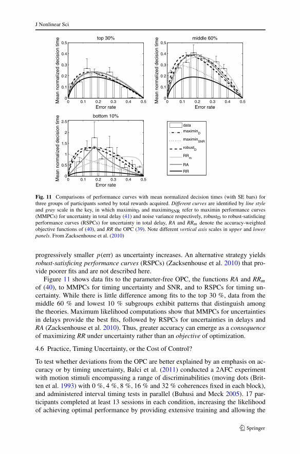
Fig. 11 Comparisons of performance curves with mean normalized decision times (with SE bars) forthree groups of participants sorted by total rewards acquired. Different curves are identified by line styleand gray scale in the key, in which maximinD and maximinSNR refer to maximin performance curves(MMPCs) for uncertainty in total delay (41) and noise variance respectively, robustD to robust-satisficingperformance curves (RSPCs) for uncertainty in total delay, RA and RRm denote the accuracy-weightedobjective functions of (40), and RR the OPC (39). Note different vertical axis scales in upper and lowerpanels. From Zacksenhouse et al. (2010)

progressively smaller p(err) as uncertainty increases. An alternative strategy yieldsrobust-satisficing performance curves (RSPCs) (Zacksenhouse et al. 2010) that pro-vide poorer fits and are not described here.

Figure 11 shows data fits to the parameter-free OPC, the functions RA and RRm

of (40), to MMPCs for timing uncertainty and SNR, and to RSPCs for timing un-certainty. While there is little difference among fits to the top 30 %, data from themiddle 60 % and lowest 10 % subgroups exhibit patterns that distinguish amongthe theories. Maximum likelihood computations show that MMPCs for uncertaintiesin delays provide the best fits, followed by RSPCs for uncertainties in delays andRA (Zacksenhouse et al. 2010). Thus, greater accuracy can emerge as a consequenceof maximizing RR under uncertainty rather than an objective of optimization.

4.6 Practice, Timing Uncertainty, or the Cost of Control?

To test whether deviations from the OPC are better explained by an emphasis on ac-curacy or by timing uncertainty, Balci et al. (2011) conducted a 2AFC experimentwith motion stimuli encompassing a range of discriminabilities (moving dots (Brit-ten et al. 1993) with 0 %,4 %,8 %,16 % and 32 % coherences fixed in each block),and administered interval timing tests in parallel (Buhusi and Meck 2005). 17 par-ticipants completed at least 13 sessions in each condition, increasing the likelihoodof achieving optimal performance by providing extensive training and allowing the

J Nonlinear Sci

Fig. 12 Mean normalized decision times (dots) grouped by coherence vs. error proportions for sessions1 (highest points and curve, red), 2–5 (second highest points and curve, blue), 6–9 (green) and 10–13(pink). Data points and fitted curves for sessions 6–13 are very similar. (a) Performance compared withOPC (lowest curve, black) and best-fitting MMPCs for each coherence condition. Performance convergestoward the OPC, but DTs remain high for p(err) > 0.35. (b) Performance compared with DD fits tosingle threshold for all coherences. Solid and dotted horizontal lines connect model fits and dotted verticallines connect data points from different sessions having the same coherence. Fits connected by solid linesexclude 0 and 4 % coherences; fits connected by dotted lines include all coherences. Single threshold fitscapture longer DTs at high error rates better than OPC and MMPCs. Panel (b) adapted from Balci et al.(2011) (Color figure online)

study of practice effects (Dutilh et al. 2009; Petrov et al. 2011). There were four mainfindings.

First, average performance converges toward the OPC with increasing experience.Figure 12(a) shows mean normalized decision times (dots) for five error bins averagedover sessions 1, 2–5, 6–9 and 10–13. Performance during the final two sets of sessionsis indistinguishable from the OPC for higher coherences, but decision times remainsignificantly above the OPC for 0 and 4 % coherences.

Second, the accuracy-weighted objective function RRm of (40) outperforms theOPC in fitting decision times, with accuracy weight decreasing monotonicallythrough sessions 1–9 and thereafter remaining at q ≈ 0.2 (not shown here, see Balciet al. (2011, Fig. 9)), suggesting that participants may initially favor accuracy, butthat this diminishes with practice.

Third, timing inaccuracy throughout all but the first session, independently as-sessed by participants’ coefficients of variation in a peak-interval task, is significantlycorrelated with their distances from the OPC (Balci et al. 2011). Moreover, this pro-vides a better account of deviations from the OPC than weighting accuracy by theparameter q in RRm, supporting the hypothesis that humans can learn to maximizerewards by devaluing accuracy, with a deviation from optimality inversely relatedto their timing ability. However, even after long practice, MMPCs based on timinguncertainty fail to capture performance for the two lowest coherences (Fig. 12(a)),suggesting that other factors may be involved, including the cost of cognitive con-trol (Posner and Snyder 1975).

To test this fourth possibility, Balci et al. (2011) computed the single optimalthreshold over all coherence conditions. Figure 12(b) shows that the resulting curve

J Nonlinear Sci

fits the full range of data for later sessions (6–13), suggesting that, given practice,participants adopted such a threshold. Rewards for this single threshold differed littlefrom those for thresholds optimized for each coherence condition, suggesting thatparticipants may seek one threshold that does best over all conditions, avoiding es-timation of coherences and control of thresholds from block to block. Control costsare discussed in Holmes and Cohen (2014).

4.7 Prior Expectations and Trial-to-Trial Adjustments

Given prior information on the probabilities of observing each stimulus in a 2AFCtask, a DD process can be optimized by appropriately shifting the initial conditionx(0); rewards that favor one response over the other can be treated similarly (Bo-gacz et al. 2006). Comparisons of these predictions with human behavioral data werecarried out in Simen et al. (2009), finding that participants achieved 97–99 % ofmaximum reward. A related study of monkeys used a fixed stimulus presentation pe-riod that obviates the need for a speed-accuracy tradeoff, but in which differencesin rewards for the two responses were signaled before each trial and motion coher-ences varied randomly between trials. The animals achieved 98 % and 99.5 % ofmaximum rewards (Feng et al. 2009), and fits of LIP recordings to an accumulatormodel (Gao et al. 2011) indicated that this was also done by shifting initial condi-tions. Human behavioral studies revealed similar near-optimal shifts in response tobiased rewards (Gao et al. 2011).

Humans also exhibit adjustment effects in response to repetition and alternationpatterns that necessarily occur, given stimuli chosen with equal probability (Soetenset al. 1985). Accumulator models developed in Cho et al. (2002), Jones et al. (2002),Gao et al. (2009), Goldfarb et al. (2012) indicate that this is also due to initial condi-tion shifts, presumably due to expectations that patterns will persist even when stimuliare purely random. In fact pattern recognition is advantageous in natural situations, al-lowing prior beliefs to adapt to match stationary or slowly changing environments (Yuand Cohen 2009).

The work described in this section depends on simple models that at first reproduceprevious data, then predict outcomes of new experiments, and finally admit analysesand modifications that account for differences between predictions and the new data.The explicit OPC expression (39) is crucial here; it seems unlikely that such predic-tions could readily emerge from computational simulations alone. These models arecertainly useful, but they do not immediately connect to cellular-level descriptionssuch as those of Sects. 2–3. We now discuss this connection.

5 Connecting the Levels

The accumulator models of Sect. 4 address optimality constraints at the systems level,but they are too abstract to identify mechanisms or constraints arising from underly-ing neural circuits. To do this the abstract models must be related to biophysicalaspects of neural function. For example, spiking-neuron models can be reduced indimension by averaging over populations of cells (Brunel and Wang 2001; Wong

J Nonlinear Sci

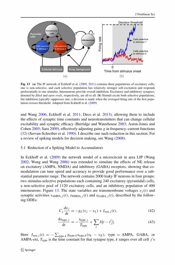
Fig. 13 (a) The IF network of Eckhoff et al. (2009, 2011) contains three populations of excitatory cells;one is non-selective, and each selective population has relatively stronger self-excitation and respondspreferentially to one stimulus. Interneurons provide overall inhibition. Excitatory and inhibitory synapses,denoted by filled and open ovals, respectively, are all to all. (b) Stimuli excite both selective populations,but inhibition typically suppresses one; a decision is made when the averaged firing rate of the first popu-lation crosses threshold. Adapted from Eckhoff et al. (2009)

and Wang 2006; Eckhoff et al. 2011; Deco et al. 2013), allowing them to includethe effects of synaptic time constants and neurotransmitters that can change cellularexcitability and synaptic efficacy (Berridge and Waterhouse 2003; Aston-Jones andCohen 2005; Sara 2009), effectively adjusting gains g in frequency–current functions(32) (Servan-Schreiber et al. 1990). I describe one such reduction in this section. Fora review of spiking models for decision making, see Wang (2008).

5.1 Reduction of a Spiking Model to Accumulators

In Eckhoff et al. (2009) the network model of a microcircuit in area LIP (Wang2002; Wong and Wang 2006) was extended to simulate the effects of NE releaseon excitatory (AMPA, NMDA) and inhibitory (GABA) receptors, showing that co-modulation can tune speed and accuracy to provide good performance over a sub-stantial parameter range. The network contains 2000 leaky IF neurons in four groups:two stimulus-selective populations each containing 240 excitatory (pyramidal) cells,a non-selective pool of 1120 excitatory cells, and an inhibitory population of 400interneurons: Figure 13. The state variables are transmembrane voltages vj (t) andsynaptic activities sAMPA,j (t), sNMDA,j (t) and sGABA,j (t), described by the follow-ing ODEs:

Cj

dvj

dt= −gL(vj − vL) + Isyn,j (t), (42)

dstype,j

dt= − stype,j

Ttype+

∑l

δ(t − t lj

). (43)

Here Isyn,j (t) = −∑type,k gtype,kstype,k(vk − vE), type = AMPA, GABA, or

AMPA-ext, Ttype is the time constant for that synapse type, k ranges over all cell j ’s

J Nonlinear Sci

presynaptic neurons, and superscripts l index times t lj at which the j th cell crossesa threshold vth, emits a delta function and is reset to vr for a refractory period τref,cf. Sect. 2.3 and Fig. 5. The NMDA dynamics require two ODEs to model fast risefollowed by slow decay (Eckhoff et al. 2011), cf. Sect. 2.5:

dsNMDA,j (t)

dt= − sNMDA,j (t)

τNMDA,decay+ αxj (t)

[1 − sNMDA,j (t)

], (44)

dxj (t)

dt= − xj (t)

τNMDA,rise+

∑l

δ(t − t lj

). (45)

External inputs sAMPA-ext,j (t), modeled by OU processes driven by Gaussiannoise of mean μ and standard deviation σ , enter all cells:

dsAMPA-ext,j = − (sAMPA-ext,j − μ)dt

τAMPA+ σ dWj . (46)

Stimuli are represented by modified mean inputs μ(1 ± E) to the selective cells withappropriately adjusted variances σj , where E ∈ [0,1] denotes stimulus discriminabil-ity (E = 1 for high SNR; E = 0 for zero SNR). Neuromodulation is represented bymultiplying excitatory and inhibitory conductances gAMPA,k, gNMDA,k and gGABA,k

by factors γE , γI . Eliminating irrelevant stype,j ’s (excitatory neurons do not releaseGABA, inhibitory neurons do not release AMPA or NMDA), (42–46) constitute a9200-dimensional hybrid, stochastic dynamical system that is analytically intractableand computationally demanding.

Following the mean-field method of Brunel and Wang (2001), Renart et al. (2003),Wong and Wang (2006), the network is first reduced to four populations by assum-ing a fixed average voltage v = (vr + vth)/2 to estimate synaptic currents. Theseare multiplied by the appropriate numbers Nj of presynaptic cells in each popula-tion and by averaged synaptic variables stype,j , and summed to create input currentsItype,j to each population (the index j ∈ {1,2,3,4} now denotes the population). In-dividual, evolving cell voltages are replaced by population-averaged, time-dependentfiring rates determined by frequency–current (f–I) curves ϕj (Isyn,j ), analogous to theinput–output function of (32). This yields an 11-dimensional system described by 4firing rates νj (t), one inhibitory population-averaged synaptic variable sGABA(t), andtwo variables sAMPA,j (t) and sNMDA,j (t) for each excitatory subpopulation (6 in all).

Further reduction to two populations relies on time scale separation (Jones 1994;Guckenheimer and Holmes 1983). Time constants for AMPA and GABA are fast(TAMPA = 2 ms, TGABA = 5 ms), while that for NMDA decay is slow (TNMDA = 100ms); sAMPA,j (t) and sGABA,j (t) therefore rapidly approach quasi-steady states, asin Rinzel’s reduction of HH in Sect. 2.2, This eliminates 3 ODEs for the excitatorypopulations and 1 for the inhibitory population. Firing rates likewise track values setby the f–I curves, since they are determined by TAMPA:

dνj

dt= −(νj − ϕj (Isyn,j ))

TAMPA, (47)

so νj (t) ≈ ϕj (Isyn,j (t)) for the non-selective and interneuron populations and theODEs for ν3 and νI drop out. Also, with stimuli on, the non-selective population

J Nonlinear Sci

Fig. 14 Contour maps of RR over the (γE,γI )-neuromodulation plane for the full network (a) and reduced2-population system (b). Inhibition dominates at upper left where excitatory cells rarely exceed threshold,at lower right excitation dominates and thresholds are rapidly crossed, giving high error rates; a ridge ofhigh RRs separates these low RR regions. From Eckhoff et al. (2011) (Color figure online)

typically has a less variable firing rate than the selective populations, so that sNMDA,3can be fixed, leaving four ODEs for the synaptic variables and firing rates of theselective populations:

dsj

dt= − sj

TNMDA+ 0.641(1 − sj )

νj

1000, (48)

dνj

dt= −νj − ϕj (Isyn,j )

Tpopf

; j = 1,2, (49)

where we write sNMDA,j = sj for brevity.2 The sj (t)’s and the firing rates νj (t) cor-respond to the activity levels xj (t) in the LCA (30–31), and white noise is added asin those SDEs.

To complete the reduction, currents must be estimated self-consistently. This iscomplicated by the fact that Isyn,j in (49) contains terms that depend on both sj andϕj (Isyn,j ), so that the vector field is defined recursively. Ideally, we seek relation-ships of the form Isyn,j = αj1s1 + αj2s2 + βj1ν1 + βj2ν2 + Iconst,j , as in Wong andWang (2006). Piecewise-smooth f–I curves help here (Eckhoff et al. 2011), sincethey predict critical currents beyond which firing rates rise linearly. The parametersγE,γI enter via the AMPA, NMDA and GABA components of the currents Iconst,jand coefficients αjk,βjk . See Eckhoff et al. (2011) for details.

Computations of reward rates over the neuromodulation plane verify that (48–49) capture key properties of the full spiking model: Fig. 14. Bifurcation diagrams(Fig. 15) reveal that up to nine fixed points, including four sinks, can coexist, asshown in the phase-plane projections of Fig. 16. The linear and approximatelyparabolic components of each nullcline derive from sub- and super-threshold parts of

2Division by 103 accommodates the conventional units of millivolts, nanoamps, and nanosiemens forconductances.

J Nonlinear Sci

Fig. 15 Bifurcation diagrams for the noise-free 2-population model for (γE,γI ) = (1,1) with E = 0 (a)and E = 0.128 (b), showing s1 vs. stimulus strength μ. Pitchfork bifurcations and pairs of saddle-nodesoccur for E = 0 (a), finite coherence breaks the symmetry (b). Only the upper- and lower-most branchesare stable, cf. Fig. 16

Fig. 16 Dynamics of the 2-population model projected onto (s1, s2) plane, with ˙s1 = 0 nullcline verticalline and curve with maximum at top (orange), ˙s2 = 0 nullcline horizontal line and curve with maximum atright (green), sinks as filled circles, saddles with one- and two-dimensional stable manifolds as open tri-angles and open circles. From top left clockwise, nullclines, fixed points, and sample trial paths are shownwithout stimulus at (γE,γI ) = (1,1), with stimulus and E = 0 (symmetric) at (γE,γI ) = (1,1), withoutstimulus at (γE,γI ) = (2,1.2), and with stimulus for E = 0.128 at (γE,γI ) = (1,1). From Eckhoff et al.(2011) (Color figure online)

the f–I curves ϕj (Isyn,j ), as described in Eckhoff et al. (2011). In the top two and bot-tom left panels of Fig. 16 (γE, γI ) = (1,1) (on the RR ridge of Fig. 14(b)) cases with-

J Nonlinear Sci

out stimulus, with identical stimuli E = 0,SNR = 0 and with E = 0.128,SNR > 0are shown. States with both sj ’s low represent lack of response, possibly awaitingstimulus appearance. With stimuli present, the basin of attraction of the low-low sinkshrinks, allowing noisy trials to reach the choice attractors s1 � s2 and s2 � s1, asin Wong and Wang (2006); the basin of the correct attractor is larger for E > 0 (bot-tom left panel). Finally, for (γE, γI ) = (2,1.2) (lower right region in Fig. 14(b) andFig. 16, bottom right panel), s1, s2 both high corresponds to impulsive behavior inwhich near-random choices occur.

5.2 Physiological Constraints to Optimality?

The global dynamics of the reduced system (48–49), with its multiple attractors(Fig. 16), differs qualitatively and quantitatively from the optimal DD process of (34).While the dynamics near a saddle point approximate the approach of orbits to a driftalong one-dimensional DD dynamics, acceleration away from the saddle and decel-eration toward an attractor cause suboptimal integration. Moreover, even if an attract-ing one-dimensional subspace exists, deviations from it effectively blur the decisionthresholds, and firing rate bounds preclude negative and arbitrarily high activations,preventing perfect subtraction as in (33) (van Ravenzwaaij et al. 2012, Figs. 5–7).Adjustments in baseline activity and gain can keep accumulator states in near-lineardynamical ranges (Servan-Schreiber et al. 1990; Cohen et al. 1990), but the fact thatnonlinear dynamics emerge from a biophysically based model suggests physiologicalobstructions to optimality, especially when task conditions span a wide range (Decoet al. 2013).

In this regard it is worth noting that choice attractors such as those of Fig. 16,which can persist in the absence of stimuli (Fig. 15(a)), have been identified withshort-term working memory states (Usher and Cohen 1999; Wang 1999; Renart et al.2003; Wong and Wang 2006; Deco et al. 2013). Working memory is clearly importantfor delayed-response tasks such as those of Zhang and Barash (2004), Feng et al.(2009), Rorie et al. (2010), Gao et al. (2011) and in many other aspects of our lives.It is therefore plausible that cortical circuits have evolved to allow flexible multi-attractor dynamics that are inconsistent with optimal strategies in artificially simpletasks such as 2AFC.

6 Discussion: Some Omissions and Open Problems

In this article I have outlined some mathematical models in neuroscience that drawon dynamical systems theory. Specifically, Sects. 2–3 describe mechanistic, cellular-scale models for the generation of action potentials (spikes) and for electrical andchemical synapses, discuss methods for reducing their dimension and hence simplify-ing their analysis, and illustrate with a model of a central pattern generator for leggedlocomotion. This represents the dominant approach to modeling among neuroscien-tists and applied mathematicians. In contrast, Sect. 4 takes a high level perspective,using stochastic ODEs and a drift-diffusion (DD) model to represent accumulation ofevidence in brain areas and to predict a strategy for maximizing reward rate in binaryperceptual choice tasks, enabled by the simplicity of the DD model. Such models

J Nonlinear Sci

exemplify the connectionist neural networks in wide use among cognitive psycholo-gists. They can be justified empirically by their ability to fit behavioral data, and, moredirectly, from observations of spike rates in animal studies. They can also be derived,albeit non-rigorously, from cellular-scale spiking models, as sketched in Sect. 5.

These models illustrate the range of scales and models in mathematical neuro-science, but as noted in Sect. 1, many important ideas and approaches are miss-ing from this account. While spinal and thoracic CPGs generate functional motorrhythms, brains exhibit cortical oscillations over a wide frequency range (2–100 Hz),as detected via electroencephalography (scalp electrodes) and extracellular electrodesrecording local field potentials (Buzsaki 2006; Baker 2007; Fries et al. 2007). Thereis much debate about the mechanisms and functions of such oscillations (Kopell et al.2009; Whittington et al. 2009; Wang 2010), including their rôles in “binding” differ-ent sensory modalities (Gray et al. 1989; Gray and Singer 1995; Fries 2005) and indiseased states (McCarthy et al. 2011, 2012; Uhlhaas and Singer 2010), and theirgeneration by and effects on spikes from individual cells (Wang 2010). Further mod-eling, with phase oscillators as well as HH-type equations, could shed light on thesecortical rhythms.

The study of how organisms learn about and adapt to changing environments is amajor area in which reinforcement learning (RL) (Sutton 1988; Sutton and Barto1998) and the extended notion of hierarchical reinforcement learning (Botvinicket al. 2009; Botvinick 2012) draw on studies of the dopamine neuromodulation sys-tem (Schultz et al. 1997, 2000) to propose discrete dynamical updates followingrewarded behaviors. Dimension reduction can occur in RL (Swinehard and Abbott2006). Goal-directed planning and searching also employ iterative models in whichdifferent strategies are explored (Solway and Botvinick 2012). On the mechanisticlevel, cortical rhythms also may be important in learning (Torta et al. 2009).

Probabilistic ideas are also widely used, perhaps more widely than those fromdynamical systems. An influential subculture considers probabilistic computationsbased on Bayes’ rule (Bayes 1763) that offer normative accounts of task performanceas dynamic updating of priors. Models have been developed for sensori-motor con-trol, e.g. Kording et al. (2004), Kording and Wolpert (2006), Wolpert (2007), andproposed to describe stimulus identification, decision making and learning (Knill andPouget 2004; Liu et al. 2009; Yu et al. 2009; Bejjanki et al. 2011; Dayan 2012; Sol-way and Botvinick 2012). These models are mostly empirical, but there is increasingevidence that the brain can code probability distributions and perform Bayesian com-putations, possibly via cortico-basal ganglia circuits (Pouget et al. 2003; Knill andPouget 2004; Ma et al. 2006, 2008; Bogacz and Gurney 2007; Bogacz and Larsen2011; Coulthard et al. 2012). Information theory (Shannon 1948), originally sug-gested by Weiner as a descriptor for sensory receptors (Wiener 1948, especiallyChap. III) has also been used to analyze spike trains and quantify their informationcontent in attempts to understand neural coding (Rieke et al. 1997, Chap. 3) as wellas learning (MacKay 2003). More generally, probabilistic methods including hiddenMarkov models are useful in analyzing multi-electrode recordings in terms of transi-tions among brain states, e.g. Seidemann et al. (1996), Gervasoni et al. (2004), Joneset al. (2007).

In closing I note some open problems, focusing on ones that arise from the modelsdiscussed in Sects. 2–5. A persistent difficulty is in identifying brain areas and neu-

J Nonlinear Sci

ral substrates in which specific “computations” are done. Excepting some specializedsensory and sensori-motor circuits, such as those dedicated to reflexive actions, mostcomputations appear to activate multiple brain areas. For example, while neural firingrates in area LIP are similar to DD processes (Shadlen and Newsome 2001; Roitmanand Shadlen 2002), pharmacological inactivation of LIP may not deprive an animalof the ability to identify stimuli and respond appropriately (Balan and Gottlieb 2009)(although it may slow him down). Computational models involving multiple brainareas have been constructed for over 30 years (Rumelhart and McClelland 1986), butthere have been few attempts to analyze them mathematically (an exception is Liuet al. (2008), which shows that the multi-layer network of Cohen et al. (1992) can bereduced to a DD process with time-varying input). Moreover, until recently simul-taneous neural recordings from multiple areas have not been available to constrainmulti-area models.

Here are suggestions some specific things to pursue:

• Improved theory and analytical methods for hybrid dynamical systems, especially(large) networks of integrate-and-fire cells.

• Better descriptions of, and methods for extracting macroscopic activity states inaveraging over large cell populations.

• Nested sets of models for simple tasks, fitted to electrophysiological and behavioraldata.

• Further use of time scale separation in creating and analyzing models of cognitivedynamics.

• Analyses of iterative learning algorithms as dynamical systems.

The joys celebrated herein are chiefly in the works of others, the trials come in myattempts to understand them, and to contribute new ideas.

Acknowledgements This article draws upon work done since 2000, variously supported by NSF underDMS-0101208 and EF-0425878, AFOSR under FA9550-07-1-0537 and FA9550-07-1-0528, NIH underP50 MH62196, the US-Israel Binational Science Foundation under BSF 2011059, and the J. Insley PyneFund of Princeton University. The material in Sects. 2–3 was adapted from notes for a course taught atPrinceton since 2006 to which Philip Eckhoff contributed much. An extended version of Sect. 4 appearsin Holmes and Cohen (2014). The author thanks Fuat Balci for providing Fig. 12 and the anonymousreviewers for their suggestions, and gratefully acknowledges the contributions of many other collaborators,not all of whose work could be cited here.

References

Abbott, L.F.: Theoretical neuroscience rising. Neuron 60, 489–495 (2008)Arnold, L.: Stochastic Differential Equations. Wiley, New York (1974)Aston-Jones, G., Cohen, J.D.: An integrative theory of locus coeruleus-norepinephrine function: adaptive

gain and optimal performance. Annu. Rev. Neurosci. 28, 403–450 (2005)Ayali, A., Fuchs, E., Hulata, E., Jacob, E.B.: The function of inter segmental connections in determining

temporal characteristics of the spinal cord rhythmic output. Neuroscience 147, 236–246 (2007)Back, A., Guckenheimer, J., Myers, M.: A dynamical simulation facility for hybrid systems. In: Lecture

Notes in Computer Science, vol. 736, pp. 255–267. Springer, Berlin (1993)Baker, S.N.: Oscillatory interactions between sensorimotor cortex and periphery. Curr. Opin. Neurobiol.

17, 649–655 (2007)Balan, P.F., Gottlieb, J.: Functional significance of nonspatial information in monkey lateral intraparietal

area. J. Neurosci. 29(25), 8166–8176 (2009)

J Nonlinear Sci

Balci, F., Simen, P., Niyogi, R., Saxe, A., Holmes, P., Cohen, J.D.: Acquisition of decision making criteria:reward rate ultimately beats accuracy. Atten. Percept. Psychophys. 73(2), 640–657 (2011)

Bayes, T.: An essay toward solving a problem in the doctrine of chances. Philos. Trans. R. Soc. Lond. 53,370–418 (1763)

Bejjanki, V.R., Lu, Z.L., Beck, J.M., Pouget, A.: Perceptual learning as improved probabilistic inferencein early sensory areas. Nat. Neurosci. 14(6), 783–790 (2011)

Ben-Haim, Y.: Information Gap Decision Theory: Decisions Under Severe Uncertainty, 2nd edn. Aca-demic Press, New York (2006)

Berridge, C.W., Waterhouse, B.D.: The locus coeruleus-noradrenergic system: modulation of behavioralstate and state-dependent cognitive processes. Brains Res. Rev. 42, 33–84 (2003)

Bogacz, R., Gurney, K.: The basal ganglia and cortex implement optimal decision making between alter-native actions. Neural Comput. 19, 442–477 (2007)

Bogacz, R., Larsen, T.: Integration of reinforcement learning and optimal decision-making theories of thebasal ganglia. Neural Comput. 23, 817–851 (2011)

Bogacz, R., Brown, E., Moehlis, J., Holmes, P., Cohen, J.D.: The physics of optimal decision making:a formal analysis of models of performance in two alternative forced choice tasks. Psychol. Rev.113(4), 700–765 (2006)

Bogacz, R., Hu, P., Holmes, P., Cohen, J.D.: Do humans produce the speed-accuracy tradeoff that maxi-mizes reward rate? Q. J. Exp. Psychol. 63(5), 863–891 (2010)

Bohil, C.J., Maddox, W.T.: On the generality of optimal versus objective classifier feedback effects ondecision criterion learning in perceptual categorization. Mem. Cogn. 31(2), 181–198 (2003)

Botvinick, M.M.: Hierarchical reinforcement learning and decision making. Curr. Opin. Neurobiol. 22,956–962 (2012)

Botvinick, M.M., Niv, Y., Barto, A.C.: Hierarchically organized behavior and its neural foundations:a reinforcement-learning perspective. Cognition 113, 262–280 (2009)

Britten, K.H., Shadlen, M.N., Newsome, W.T., Movshon, J.A.: Responses of neurons in macaque MT tostochastic motion signals. Vis. Neurosci. 10, 1157–1169 (1993)

Brown, E., Moehlis, J., Holmes, P.: On the phase reduction and response dynamics of neural oscillatorpopulations. Neural Comput. 16(4), 673–715 (2004)

Brown, E., Gao, J., Holmes, P., Bogacz, R., Gilzenrat, M., Cohen, J.: Simple networks that optimize deci-sions. Int. J. Bifurc. Chaos 15(3), 803–826 (2005)

Brunel, N., van Rossum, M.C.W.: Lapicque’s 1907 paper: from frongs to integrate-and-fire. Biol. Cybern.97, 337–339 (2007)

Brunel, N., Wang, X.-J.: Effects of neuromodulation in a cortical network model. J. Comput. Neurosci. 11,63–85 (2001)

Buchanan, J.T., Grillner, S.: Newly identified glutamate interneurons and their role in locomotion in thelamprey spinal cord. Science 236, 312–314 (1987)

Buhusi, C.V., Meck, W.H.: What makes us tick? Functional and neural mechanisms of interval timing.Nature 6, 755–765 (2005)

Burkitt, A.N.: A review of the integrate-and-fire neuron model: I. Homogeneous synaptic input. Biol.Cybern. 95, 1–19 (2006a)

Burkitt, A.N.: A review of the integrate-and-fire neuron model: II. Inhomogeneous synaptic input andnetwork properties. Biol. Cybern. 95, 97–112 (2006b)

Busemeyer, J.R., Townsend, J.T.: Decision field theory: a dynamic-cognitive approach to decision makingin an uncertain environment. Psychol. Rev. 100, 432–459 (1993)

Buzsaki, G.: Rhythms of the Brain. Oxford University Press, New York (2006)Chay, T.R., Keizer, J.: Minimal model for membrane oscillations in the pancreatic β-cell. Biophys. J. 42,

181–190 (1983)Chiel, H.J., Beer, R.D.: The brain has a body: adaptive behavior emerges from interactions of nervous

system, body and environment. Trends Neurosci. 20(12), 553–557 (1997)Cho, R.Y., Nystrom, L.E., Brown, E., Jones, A.D., Braver, T.S., Holmes, P., Cohen, J.D.: Mechanisms

underlying dependencies of performance on stimulus history in a two-alternative forced-choice task.Cogn. Affect. Behav. Neurosci. 2(4), 283–299 (2002)

Chung, K., Wallace, J., Kim, S.-Y., Kalyanasundaram, S., Andalman, A.S., Davidson, T.J., Mirzabekov,J.J., Zalocusky, K.A., Mattis, J., Denisin, A.K., Pak, S., Bernstein, H., Ramakrishnan, C., Grosenick,L., Gradinaru, V., Deisseroth, K.: Structural and molecular interrogation of intact biological systems.Nature 497, 332–337 (2013)

J Nonlinear Sci

Cohen, A.H., Holmes, P., Rand, R.H.: The nature of coupling between segmental oscillators of the lampreyspinal generator for locomotion: a model. J. Math. Biol. 13, 345–369 (1982)

Cohen, A.H., Rossignol, S., Grillner, S. (eds.): Neural Control of Rhythmic Movements in Vertebrates.Wiley, New York (1988)

Cohen, J.D., Dunbar, K., McClelland, J.L.: On the control of automatic processes: a parallel distributedprocessing model of the Stroop effect. Psychol. Rev. 97(3), 332–361 (1990)

Cohen, J.D., Servan-Schreiber, D., McClelland, J.L.: A parallel distributed processing approach to auto-maticity. Am. J. Psychol. 105, 239–269 (1992)

Coulthard, E.J., Bogacz, R., Javed, S., Mooney, L.K., Murphy, G., Keeley, S., Whone, A.L.: Distinctroles of dopamine and subthalamic nucleus in learning and probabilistic decision making. Brain 135,3721–3734 (2012)

Daun-Gruhn, S.: A mathematical modeling study of inter-segmental coordination during stick insect walk-ing. J. Comput. Neurosci. 30(2), 255–278 (2011)

Daun-Gruhn, S., Toth, T.I.: An inter-segmental network model and its use in elucidating gait-switches inthe stick insect. J. Comput. Neurosci. 31(1), 43–60 (2011)

Daun-Gruhn, S., Rubin, J.E., Rybak, I.A.: Control of oscillation periods and phase durations in half-centercentral pattern generators: a comparative mechanistic analysis. J. Comput. Neurosci. 27(1), 3–36(2009)

Dayan, P.: How to set the switches on this thing. Curr. Opin. Neurobiol. 22, 1068–1074 (2012)Dayan, P., Abbott, L.F.: Theoretical Neuroscience: Computational and Mathematical Modeling of Neural

Systems. MIT Press, Cambridge (2001)De Schutter, E.: Why are computational neuroscience and systems biology so separate? PLoS Comput.

Biol. 4(5), e1000078 (2008)De Schutter, E. (ed.): Computational Modeling Methods for Neuroscientists. MIT Press, Cambridge

(2009)Deco, G., Rolls, E.T., Albantakis, L., Romo, R.: Brain mechanisms for perceptual and reward-related

decision-making. Prog. Neurobiol. 103, 194–213 (2013)Destexhe, A., Mainen, Z.F., Sejnowski, T.J.: Kinetic models of synaptic transmission. In: Koch, C., Segev,

I. (eds.) Methods in Neuronal Modeling: From Ions to Networks, 2nd edn., pp. 1–25. MIT Press,Cambridge (1999)

Doloc-Mihu, A., Calabrese, R.L.: A database of computational models of a half-center oscillator for ana-lyzing how neuronal parameters influence network activity. J. Biol. Phys. 37(3), 263–283 (2011)

Doya, K., Shadlen, M.N. (eds.): Decision making. Curr. Opin. Neurobiol. 22(6) (2012). Special issueDutilh, G., Vandekerckhove, J., Tuerlinckx, F., Wagenmakers, E.J.: A diffusion model decomposition of

the practice effect. Psychon. Bull. Rev. 16(6), 1026–1036 (2009)Eckhoff, P., Wong-Lin, K.F., Holmes, P.: Optimality and robustness of a biophysical decision-making

model under nonepinephrine modulation. J. Neurosci. 29(13), 4301–4311 (2009)Eckhoff, P., Wong-Lin, K.F., Holmes, P.: Dimension reduction and dynamics of a spiking neuron model

for decision making under neuromodulation. SIAM J. Appl. Dyn. Syst. 10(1), 148–188 (2011)Ermentrout, G.B., Kopell, N.: Parabolic bursting in an excitable system coupled with a slow oscillation.

SIAM J. Appl. Math. 46, 233–253 (1986)Ermentrout, G.B., Terman, D.: Mathematical Foundations of Neuroscience. Springer, New York (2010)Feng, S., Holmes, P., Rorie, A., Newsome, W.T.: Can monkeys choose optimally when faced with noisy

stimuli and unequal rewards? PLoS Comput. Biol. 5(2), e1000284 (2009)FitzHugh, R.: Impulses and physiological states in models of nerve membrane. Biophys. J. 1, 445–466

(1961)Foucaud-Trocme, N., Brunel, N.: Dynamics of the instantaneous firing rate in response to changes in input

statistics. J. Comput. Neurosci. 18, 311–321 (2005)Foucaud-Trocme, N., Hansel, D., van Vreeswijk, C., Brunel, N.: How spike generation mechanisms deter-

mine the neuronal response to fluctuating inputs. J. Neurosci. 23, 11628–11640 (2003)Fries, P.: A mechanism for cognitive dynamics: neuronal communication through neuronal coherence.

Trends Cogn. Sci. 9, 474–480 (2005)Fries, P., Nikolic, D., Singer, W.: The gamma cycle. Trends Neurosci. 30, 309–316 (2007)Fuchs, E., Holmes, P., Kiemel, T., Ayali, A.: Intersegmental coordination of cockroach locomotion: adap-

tive control of centrally coupled pattern generator circuits. Frontiers Neural Circuits 4, 125 (2011)Gabbiani, F., Cox, S.: Mathematics for Neuroscientists. Academic Press, San Diego (2010)Gao, J., Wong-Lin, K.F., Holmes, P., Simen, P., Cohen, J.D.: Sequential effects in two-choice reaction time

tasks: decomposition and synthesis of mechanisms. Neural Comput. 21(9), 2407–2436 (2009)

J Nonlinear Sci

Gao, J., Tortell, R., McClelland, J.L.: Dynamic integration of reward and stimulus information in percep-tual decision-making. PLoS ONE 6(3), e16749 (2011)

Gardiner, C.W.: Handbook of Stochastic Methods for Physics, Chemistry and the Natural Sciences.Springer, New York (1985), 3rd edn. (2004)

Gervasoni, D., Lin, S.-C., Ribeiro, S., Soares, E.S., Pantoja, J., Nicolelis, M.A.L.: Global forebrain dy-namics predict rat behavioral states and their transitions. J. Neurosci. 24(49), 11137–11147 (2004)

Getting, P.A.: Comparative analysis of invertebrate central pattern generators. In: Cohen, A.H., Rossignol,S., Grillner, S. (eds.) Neural Control of Rhythmic Movements in Vertebrates, pp. 101–128. Wiley,New York (1988), Chap. 4

Ghigliazza, R.M., Holmes, P.: A minimal model of a central pattern generator and motoneurons for insectlocomotion. SIAM J. Appl. Dyn. Syst. 3(4), 671–700 (2004a)

Ghigliazza, R.M., Holmes, P.: Minimal models of bursting neurons: how multiple currents, conductancesand timescales affect bifurcation diagrams. SIAM J. Appl. Dyn. Syst. 3(4), 636–670 (2004b)

Gibbon, J.: Scalar expectancy theory and Weber’s law in animal timing. Psychol. Rev. 84(3), 279–325(1977)

Gold, J.I., Shadlen, M.N.: Neural computations that underlie decisions about sensory stimuli. Trends Cogn.Sci. 5(1), 10–16 (2001)

Gold, J., Shadlen, M.: Banburismus and the brain: decoding the relationship between sensory stimuli,decisions, and reward. Neuron 36, 299–308 (2002)

Gold, J.I., Shadlen, M.N.: Banburismus and the brain: decoding the relationship between sensory stimuli,decisions, and reward. Neuron 36, 299–308 (2002)

Goldfarb, S., Wong-Lin, K.F., Schwemmer, M., Leonard, N.E., Holmes, P.: Can post-error dynamics ex-plain sequential reaction time patterns? Frontiers Psychol. 3, 213 (2012)

Gray, C.M., Singer, W.: Visual feature integration and the temporal correlation hypothesis. Annu. Rev.Neurosci. 18, 555–586 (1995)

Gray, C.M., König, P., Engel, A.K., Singer, W.: Oscillatory responses in cat visual cortex exhibit inter-columnar synchronization which reflects global stimulus properties. Nature 338, 334–337 (1989)

Grillner, S.: Bridging the gap—from ion channels to networks and behaviour. Curr. Opin. Neurobiol. 9,663–669 (1999)

Grossberg, S.: Nonlinear neural networks: principles, mechanisms, and architectures. Neural Netw. 1, 17–61 (1988)

Guckenheimer, J.: Isochrons and phaseless sets. J. Math. Biol. 1, 259–273 (1975)Guckenheimer, J., Holmes, P.: Nonlinear Oscillations, Dynamical Systems and Bifurcations of Vector

Fields. Springer, New York (1983), 6th edn. (2002)Guckenheimer, J., Johnson, S.: Planar hybrid systems. In: Lecture Notes in Computer Science, vol. 999,

pp. 202–225. Springer, Berlin (1995)Hagevik, A., McClellan, A.D.: Coupling of spinal locomotor networks in larval lamprey revealed by recep-

tor blockers for inhibitory amino acids: neurophysiology and computer modeling. J. Neurophysiol.72, 1810–1829 (1994)

Hellgren, J., Grillner, S., Lansner, A.: Computer simulation of the segmental neural network generatinglocomotion in lamprey by using populations of network interneurons. Biol. Cybern. 68, 1–13 (1992)

Hill, A.A., Lu, J., Masino, M.A., Olsen, O.H., Calabrese, R.L.: A model of a segmental oscillator in theleech heartbeat neuronal network. J. Comput. Neurosci. 10, 281–302 (2001)

Hirsch, M.W., Pugh, C.C., Shub, M.: Invariant Manifolds. Springer Lecture Notes in Mathematics, vol.583. Springer, Berlin (1977)

Hirsch, M.W., Smale, S., Devaney, R.L.: Differential Equations, Dynamical Systems and an Introductionto Chaos. Academic Press/Elsevier, San Diego (2004)

Hodgkin, A.L., Huxley, A.F.: The components of membrane conductance in the giant axon of Loligo.J. Physiol. 116, 473–496 (1952a)

Hodgkin, A.L., Huxley, A.F.: Currents carried by sodium and potassium ions through the membrane of thegiant axon of Loligo. J. Physiol. 116, 449–472 (1952b)

Hodgkin, A.L., Huxley, A.F.: The dual effect of membrane potential on sodium conductance in the giantaxon of Loligo. J. Physiol. 116, 497–506 (1952c)

Hodgkin, A.L., Huxley, A.F.: A quantitative description of membrane current and its application to con-duction and excitation in nerve. J. Physiol. 117, 500–544 (1952d)

Hodgkin, A.L., Huxley, A.F., Katz, B.: Ionic currents underlying activity in the giant axon of the squid.Arch. Sci. Physiol. 3, 129–150 (1949)

J Nonlinear Sci

Hodgkin, A.L., Huxley, A.F., Katz, B.: Measurement of current-voltage relations in the membrane of thegiant axon of Loligo. J. Physiol. 116, 424–448 (1952)

Holmes, M.H.: Introduction to Perturbation Methods, 2nd edn. Springer, New York (2013)Holmes, P., Cohen, J.D.: Optimality and some of its discontents: successes and shortcomings of existing

models for binary decisions. Top. Cog. Sci. 6 (2014). To appearHolmes, P., Full, R.J., Koditschek, D., Guckenheimer, J.: The dynamics of legged locomotion: models,

analyses and challenges. SIAM Rev. 48(2), 207–304 (2006)Hoppensteadt, F.C., Izhikevich, E.M.: Weakly Connected Neural Networks. Springer, New York (1997)Ijspeert, A.J.: Central pattern generators for locomotion control in animals and robots: a review. Neural

Netw. 21, 642–653 (2008)Insel, T.R., Landis, S.C., Collins, F.S.: The NIH BRAIN initiative. Science 340(6133), 687–688 (2013)Izhikevich, E.M.: Which model to use for cortical spiking neurons? IEEE Trans. Neural Netw. 15, 1063–

1070 (2004)Johnston, D., Wu, S.: Foundations of Cellular Neurophysiology. MIT Press, Cambridge (1997)Jones, C.K.R.T.: Geometric Singular Perturbation Theory. Lecture Notes in Mathematics, vol. 1609.

Springer, Heidelberg (1994). C.I.M.E. LecturesJones, A.D., Cho, R.Y., Nystrom, L.E., Cohen, J.D., Brown, E.T., Braver, T.S.: A computational model

of anterior cingulate function in speeded response tasks: effects of frequency, sequence, and conflict.Cog. Affect. Behav. Neurosci. 2(4), 300–317 (2002)

Jones, L.M., Fontanini, A., Sadacca, B.F., Miller, P., Katz, D.B.: Natural stimuli evoke dynamic sequencesof states in sensory cortical ensembles. Proc. Natl. Acad. Sci. USA 104(47), 18772–18777 (2007)

Keener, J., Sneyd, J.: Mathematical Physiology, 2nd edn. Springer, New York (2009), 2 volsKnight, B.W.: Dynamics of encoding in a population of neurons. J. Gen. Physiol. 59, 734–766 (1972a)Knight, B.W.: The relationship between the firing rate of a single neuron and the level of activity in a

population of neurons. Experimental evidence for resonant enhancement in the population response.J. Gen. Physiol. 59, 767–778 (1972b)

Knill, D.C., Pouget, A.: The Bayesian brain: the role of uncertainty in neural coding and computation.Trends Neurosci. 27(12) (2004)

Kopell, N.: Toward a theory of modelling central pattern generators. In: Cohen, A.H., Rossignol, S., Grill-ner, S. (eds.) Neural Control of Rhythmic Movements in Vertebrates, pp. 3369–3413. Wiley, NewYork (1988)

Kopell, N., Traub, R.D., Whittington, M.A.: Modeling rhythms: from physiology to function. In: ShortCourse 2, Rhythms of the Neocortex: Where Do They Come From and What Are They Good For?Society for Neuroscience (2009). http://www.sfn.org/shortcourses

Kopell, N., Börgers, C., Pervouchine, D., Malerba, P., Tort, A.B.L.: Gamma and theta rhythms in bio-physical models of hippocampal circuits. In: Cutsuridis, V., Graham, B.F., Cobb, S., Vida, I. (eds.)Hippocampal Microcircuits: A Computational Modeller’s Resource Book, pp. 423–457. Springer,New York (2010)

Kording, K.P., Wolpert, D.M.: Bayesian decision theory in sensorimotor control. Trends Cogn. Sci. 10,319–326 (2006)

Kording, K.P., Ku, S., Wolpert, D.: Bayesian integration in force estimation. J. Neurophysiol. 92, 3161–3165 (2004)

Krinsky, V.I., Kokoz, Yu.M.: Reduction of the Hodgkin-Huxley system to a second order system. Biofizika18(3), 506–511 (1973)

Kukillaya, R.P., Holmes, P.: A hexapedal jointed-leg model for insect locomotion in the horizontal plane.Biol. Cybern. 97, 379–395 (2007)

Kukillaya, R.P., Holmes, P.: A model for insect locomotion in the horizontal plane: feedforward activationof fast muscles, stability, and robustness. J. Theor. Biol. 261(2), 210–226 (2009)

Kukillaya, R.P., Proctor, J., Holmes, P.: Neuro-mechanical models for insect locomotion: Stability, maneu-verability, and proprioceptive feedback. CHAOS: Interdiscip. J. Nonlinear Sci. 19(2), 026107 (2009)

Laming, D.R.J.: Information Theory of Choice-Reaction Times. Academic Press, New York (1968)Lapicque, L.: Recherches quantitatives sur l’excitatabilité électrique des nerfs traitée comme une polarisa-

tion. J. Physiol. Pathol. Gen. 9, 620–635 (1907)Latham, P., Brunel, N.: Firing rate of the noisy quadratic integrate-and-fire neuron. Neural Comput. 15,

2281–2306 (2003)Latham, P.E., Richmond, B.J., Nelson, P.G., Nirenberg, S.: Intrinsic dynamics in neuronal networks. I.

Theory. J. Neurophysiol. 83, 808–827 (2000)

J Nonlinear Sci

Liu, Y.S., Holmes, P., Cohen, J.D.: A neural network model of the Eriksen task: reduction, analysis, anddata fitting. Neural Comput. 20(2), 345–373 (2008)

Liu, Y.S., Yu, A.J., Holmes, P.: Dynamical analysis of Bayesian inference models for the Eriksen task.Neural Comput. 21(6), 1520–1553 (2009)

London, M., Häusser, M.: Dendritic computation. Annu. Rev. Neurosci. 28, 503–532 (2005)Ma, W.J., Beck, J.M., Latham, P.E., Pouget, A.: Bayesian inference with probabilistic population codes.

Nat. Neurosci. 9, 1432–1438 (2006)Ma, W.J., Beck, J.M., Pouget, A.: Spiking networks for Bayesian inference and choice. Curr. Opin. Neu-

robiol. 18, 217–222 (2008)MacKay, D.J.C.: Information Theory, Inference and Learning Algorithms. Cambridge University Press,

Cambridge (2003)Mackey, M.C., Santillán, M.: Andrew Fielding Huxley (1917–1952). AMS Not. 60(5), 576–584 (2013)Maddox, W.T., Bohil, C.J.: Base-rate and payoff effects in multidimensional perceptual categorization.

J. Exp. Psychol. 24(6), 1459–1482 (1998)Malkin, I.G.: Methods of Poincaré and Linstedt in the Theory of Nonlinear Oscillations. Gostexisdat,

Moscow (1949). In RussianMalkin, I.G.: Some Problems in Nonlinear Oscillation Theory. Gostexisdat, Moscow (1956). In RussianMarder, E.: Motor pattern generation. Curr. Opin. Neurobiol. 10(6), 691–698 (2000)Marder, E., Bucher, D.: Understanding circuit dynamics using the stomatogastric nervous system of lob-

sters and crabs. Annu. Rev. Physiol. 69, 291–316 (2007)Markram, H.: The blue brain project. Nat. Rev. Neurosci. 7, 153–160 (2006)Mazurek, M.E., Roitman, J.D., Ditterich, J., Shadlen, M.N.: A role for neural integrators in perceptual

decision making. Cereb. Cortex 13(11), 891–898 (2003)McCarthy, M.M., Moore-Kochlacs, C., Gu, X., Boyden, E.S., Han, X., Kopell, N.: Striatal origin of the

pathologic beta oscillations in Parkinson’s disease. Proc. Nat. Acad. Sci. 108(28), 11620–11625(2011)

McCarthy, M.M., Ching, S., Whittington, M.A., Kopell, N.: Dynamical changes in neurological diseaseand anesthesia. Curr. Opin. Neurobiol. 22(4), 693–703 (2012)

McGinn, C.: What can your neurons tell you? New York Review of Books. LX 12:49–50 (2013), by J.-P.Changeux

McMillen, T., Holmes, P.: An elastic rod model for anguilliform swimming. J. Math. Biol. 53, 843–866(2006)

McMillen, T., Williams, T.L., Holmes, P.: Nonlinear muscles, passive viscoelasticity and body taper con-spire to create neuro-mechanical phase lags in anguilliform swimmers. PLoS Comput. Biol. 4(8),e1000157 (2008)

Miller, K.D., Fumarola, F.: Mathematical equivalence of two common forms of firing rate models of neuralnetworks. Neural Comput. 24, 25–31 (2012)

Myung, J., Busemeyer, J.R.: Criterion learning in a deferred decision-making task. Am. J. Psychol. 102(1),1–16 (1989)

Nagumo, J.S., Arimoto, S., Yoshizawa, S.: An active pulse transmission line simulating a nerve axon. Proc.IRE 50, 2061–2070 (1962)

Pearson, K.G.: Central programming and reflex control of walking in the cockroach. J. Exp. Biol. 56,173–193 (1972)

Pearson, K.G.: Motor systems. Curr. Opin. Neurobiol. 10, 649–654 (2000)Pearson, K.G., Fourtner, C.R.: Non-spiking interneurons in walking system of the cockroach. J. Neuro-

physiol. 38, 33–51 (1975)Pearson, K.G., Iles, J.F.: Discharge patterns of coxal levator and depressor motoneurones of the cockroach,

Periplaneta americana. J. Exp. Biol. 52, 139–165 (1970)Pearson, K.G., Iles, J.F.: Nervous mechanisms underlying intersegmental co-ordination of leg movements

during walking in the cockroach. J. Exp. Biol. 58, 725–744 (1973)Petrov, A.A., Van Horn, N.M., Ratcliff, R.: Dissociable perceptual-learning mechanisms revealed by

diffusion-model analysis. Psychon. Bull. Rev. 18(3), 490–497 (2011)Posner, M.I., Snyder, C.R.R.: Attention and cognitive control. In: Solso, R. (ed.) Information Processing

and Cognition: The Loyola Symposium. Lawrence Erlbaum, Hillsdale (1975)Pouget, A., Dayan, P., Zemel, R.S.: Inference and computation with population codes. Annu. Rev. Neu-

rosci. 26, 381–410 (2003)Proctor, J., Holmes, P.: Reflexes and preflexes: on the role of sensory feedback on rhythmic patterns in

legged locomotion. Biol. Cybern. 2, 513–531 (2010)

J Nonlinear Sci

Rall, W.: Branching dendritic trees and motoneuron membrane resistivity. Exp. Neurol. 1(5), 491–517(1959)

Rall, W.: Theoretical significance of dendritic trees for neuronal input-output relations. In: Reiss, R. (ed.)Neural Theory and Modeling, pp. 93–97. Stanford Univ. Press, Stanford (1964)

Rall, W., Burke, R.E., Smith, T.G., Nelson, P.G., Frank, K.: Dendritic location of synapses and possiblemechanisms for the monosynaptic EPSP in motoneurons. J. Neurophysiol. 30, 1169–1193 (1967)

Ratcliff, R.: A theory of memory retrieval. Psychol. Rev. 85, 59–108 (1978)Ratcliff, R., Van Zandt, T., McKoon, G.: Connectionist and diffusion models of reaction time. Psychol.

Rev. 106(2), 261–300 (1999)Ratcliff, R., Cherian, A., Segraves, M.A.: A comparison of macaque behavior and superior colliculus

neuronal activity to predictions from models of two choice decisions. J. Neurophysiol. 90, 1392–1407 (2003)

Ratcliff, R., Hasegawa, Y.T., Hasegawa, R.P., Smith, P.L., Segraves, M.A.: Dual-diffusion model for single-cell recording data from the superior colliculus in a brightness-discrimination task. J. Neurophysiol.97, 1756–1774 (2006)

Renart, A., Brunel, N., Wang, X.-J.: Mean-field theory of recurrent cortical networks: from irregularlyspiking neurons to working memory. In: Feng, J. (ed.) Computational Neuroscience: A Comprehen-sive Approach. CRC Press, Boca Raton (2003)

Rieke, F., Bialek, W., Warland, D., De Ruyter van Steveninck, R.: Spikes: Exploring the Neural Code. MITPress, Cambridge (1997)

Rinzel, J.: Excitation dynamics: insights from simplified membrane models. Fed. Proc. 37, 2944–2946(1985)

Roitman, J., Shadlen, M.: Response of neurons in the lateral intraparietal area during a combined visualdiscrimination reaction time task. J. Neurosci. 22, 9475–9489 (2002)

Rorie, A., Gao, J., McClelland, J.L., Newsome, W.T.: Integration of sensory and reward information duringperceptual decision-making in lateral intraparietal cortex (LIP). PLoS ONE 5(2), e9308 (2010)

Roxin, A., Ledberg, A.: Neurobiological models of two-choice decision making can be reduced to a one-dimensional nonlinear diffusion equation. PLoS Comput. Biol. 4(3), e10000146 (2008)

Rumelhart, D.E., McClelland, J.L.: Parallel Distributed Processing: Explorations in the Microstructure ofCognition. MIT Press, Cambridge (1986)

Sara, S.J.: The locus coeruleus and noradrenergic modulation of cognition. Nat. Rev. Neurosci. 10, 211–223 (2009)

Schall, J.D.: Neural basis of deciding, choosing and acting. Nat. Rev. Neurosci. 2, 33–42 (2001)Schultz, W., Dayan, P., Montague, P.R.: A neural substrate of prediction and reward. Science 275, 1593–

1599 (1997)Schultz, W., Tremblay, K.L., Hollerman, J.R.: Reward processing in primate orbitofrontal cortex and basal

ganglia. Cereb. Cortex 10, 272–284 (2000)Seidemann, E., Meilijson, I., Abeles, M., Bergman, H., Vaadia, E.: Simultaneously recorded single units in

the frontal cortex go through sequences of discrete and stable states in monkeys performing a delayedlocalization task. J. Neurosci. 16(2), 752–768 (1996)

Servan-Schreiber, D., Printz, H., Cohen, J.D.: A network model of catecholamine effects: gain, signal-to-noise ratio, and behavior. Science 249, 892–895 (1990)

Seung, S.: Connectome: How the Brain’s Wiring Makes Us Who We Are. Houghton Mifflin Harcourt,New York (2012)

Shadlen, M.N., Newsome, W.T.: Neural basis of a perceptual decision in the parietal cortex (area LIP) ofthe rhesus monkey. J. Neurophysiol. 86, 1916–1936 (2001)

Shannon, C.E.: A mathematical theory of communication. Bell Syst. Tech. J. 27(3), 379–423 (1948), alsopp. 623–656. Reprinted in Shannon and Weaver (1949)

Shannon, C.E., Weaver, W.: The Mathematical Theory of Communication. University of Illinois Press,Urbana (1949)

Sherman, A., Rinzel, J., Keizer, J.: Emergence of organized bursting in clusters of pancreatic β-cells bychannel sharing. Biophys. J. 54, 411–425 (1988)

Simen, P., Contreras, D., Buck, C., Hu, P., Holmes, P., Cohen, J.D.: Reward rate optimization in two-alternative decision making: empirical tests of theoretical predictions. J. Exp. Psychol. Hum. Percept.Perform. 35(6), 1865–1897 (2009)

Smith, P.L., Ratcliff, R.: Psychology and neurobiology of simple decisions. Trends Neurosci. 27(3), 161–168 (2004)

J Nonlinear Sci

Soetens, E., Boer, L., Hueting, J.: Expectancy or automatic facilitation? Separating sequential effects intwo-choice reaction times. J. Exp. Psychol. Hum. Percept. Perform. 11, 598–616 (1985)

Solway, A., Botvinick, M.M.: Goal-directed decision making as probabilistic inference: a computationalframework and potential neural correlates. Psychol. Rev. 119, 120–154 (2012)

Stein, R.: A theoretical analysis of neuronal variability. Biophys. J. 5, 173–194 (1965)Stone, M.: Models for choice-reaction time. Psychometrika 25, 251–260 (1960)Sutton, R.: Learning to predict by the method of temporal differences. Mach. Learn. 3, 9–44 (1988)Sutton, R.S., Barto, A.G.: Reinforcement Learning. MIT Press, Cambridge (1998)Swinehard, C., Abbott, L.F.: Dimensional reduction in reward-based learning. Netw. Comput. Neural Syst.

17, 235–252 (2006)Torta, A.B.L., Komorowskie, R.W., Manns, J.R., Kopell, N.J., Eichenbaum, H.: Theta-gamma coupling in-

creases during the learning of item-context associations. Proc. Natl. Acad. Sci. USA 106(49), 20942–20947 (2009)

Toth, T.I., Daun-Gruhn, S.: A putative neuronal network controlling the activity of the leg motoneurons ofthe stick insect. NeuroReport 22(18), 943–946 (2011)

Tytell, E.D., Hsu, C.-Y., Williams, T.L., Cohen, A.H., Fauci, L.J.: Interactions between body stiffness,muscle activation, and fluid environment in a neuromechanical model of lamprey swimming. Proc.Natl. Acad. Sci. 107(46), 19832–19837 (2010)

Tytell, E.D., Holmes, P., Cohen, A.H.: Spikes alone do not behavior make: why neuroscience needs biome-chanics. Curr. Opin. Neurobiol. 21, 816–822 (2011)

Uhlhaas, P.J., Singer, W.: Abnormal neural oscillations and synchrony in schizophrenia. Nat. Rev. Neu-rosci. 11, 100–113 (2010)

Usher, M., Cohen, J.D.: Short term memory and selection processes in a frontal-lobe model. In: Heinke,D., Humphreys, G.W., Olson, A.J. (eds.) Connectionist models in cognitive neuroscience: the 5thneural computation and psychology workshop, pp. 78–91. Springer, Birmingham (1999)

Usher, M., McClelland, J.L.: On the time course of perceptual choice: the leaky competing accumulatormodel. Psychol. Rev. 108, 550–592 (2001)

van Ravenzwaaij, D., van der Maas, H.L.J., Wagenmakers, E.J.: Optimal decision making in neural inhi-bition models. Psychol. Rev. 119(1), 201–215 (2012)

Várkonyi, P.L., Kiemel, T., Hoffman, K., Cohen, A.H., Holmes, P.: On the derivation and tuning of phaseoscillator models for lamprey central pattern generators. J. Comput. Neurosci. 25, 245–261 (2008)

von Neumann, J.: The Computer and the Brain, 2nd edn. Yale University Press, New Haven (1958). Witha foreward by P.M. and Churchland P.S. (2000)

Wald, A., Wolfowitz, J.: Optimum character of the sequential probability ratio test. Ann. Math. Stat. 19,326–339 (1948)

Wallen, P., Ekeberg, O., Lansner, A., Brodin, L., Traven, H., Grillner, S.: A computer-based model forrealistic simulations of neural networks. II. The segmental network generating locomotor rhythmicityin the lamprey. J. Neurophysiol. 68, 1939–1950 (1992)

Wang, X.-J.: Synaptic basis of cortical persistent activity: the importance of NMDA receptors to workingmemory. J. Neurosci. 19, 9587–9603 (1999)

Wang, X.-J.: Probabilistic decision making by slow reverberation in cortical circuits. Neuron 36, 955–968(2002)

Wang, X.-J.: Decision making in recurrent neuronal circuits. Neuron 60, 215–234 (2008)Wang, X.-J.: Neurophysiological and computational principles of cortical rhythms in cognition. Physiol.

Rev. 90, 1195–1268 (2010)Whittington, M.A., Traub, R.D., Kopell, N.: Diverse origins of network rhythms in cortical local circuits.

In: Short Course 2, Rhythms of the Neocortex: Where do They Come From and What Are They GoodFor? Society for Neuroscience (2009). http://www.sfn.org/shortcourses

Wiener, N.: Cybernetics: Or Control and Communication in the Animal and the Machine, 2nd edn. MITPress, Cambridge (1948). 1961

Wilson, H.: Spikes, Decisions and Actions: The Dynamical Foundations of Neuroscience. Oxford Univer-sity Press, Oxford (1999)

Winfree, A.T.: The Geometry of Biological Time, 2nd edn. Springer, New York (2001)Wolpert, D.: Probabilistic models in human sensorimotor control. Hum. Mov. Sci. 26, 511–524 (2007)Wong, K.F., Wang, X.-J.: A recurrent network mechanism of time integration in perceptual decisions.

J. Neurosci. 26(4), 1314–1328 (2006)Yu, A.J., Cohen, J.D.: Sequential effects: superstition or rational behavior? In: Platt, J.C., Koller, D., Singer,

Y., Roweis, S. (eds.) Advances in Neural Information Processing Systems, vol. 21, pp. 1873–1880.

J Nonlinear Sci

MIT Press, Cambridge (2009)Yu, A.J., Dayan, P., Cohen, J.D.: Dynamics of attentional selection under conflict: toward a rational

Bayesian account. J. Exp. Psychol. Hum. Percept. Perform. 35(3), 700–717 (2009)Zacksenhouse, M., Holmes, P., Bogacz, R.: Robust versus optimal strategies for two-alternative forced

choice tasks. J. Math. Psychol. 54, 230–246 (2010)Zhang, M., Barash, S.: Persistent LIP activity in memory antisaccades: working memory for a sensorimotor

transformation. J. Neurophysiol. 91, 1424–1441 (2004)