SOME CONSIDERATIONS OF VEHICULAR DENSITY ON URBAN FREEWAYS

by

John J. Haynes Professor and Head of the Civil Engineering Department

Arlington State College - Arlington, Texas (Formerly Assistant Research Engineer - Texas)

Transportation Institute - Texas A&M University)

Research Report Number 24-6

Freeway Surveillance and Control Research Project Number 2-8-61-24

Sponsored by

The Texas Highway Department In Cooperation with the

U. S. Department of Commerce, Bureau of Public Roads

April, 1965

TEXAS TRANSPORTATION INSTITUTE Texas A&M University College Station, Texas

'

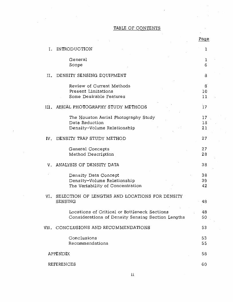
TABLE OF CONTENTS

Page

I. INTRODUCTION 1

General 1 Scope 6

II. DENSITY SENSING EQUIPMENT 8

Review of Current Methods 8 Present Limitations 10 Some Desirable Features 11

III. AERIAL PHOTOGRAPHY STUDY METHODS 17

The Houston Aerial Photography Study 17 Data Reduction 18 Density-Volume Relationship 21

IV. DENSITY TRAP STUDY METHOD 27

General Concepts 27 Method Description 28

v. ANALYSIS OF DENSITY DATA 38

Density Data Concept 38 Density-Volume Relationship 39 The Variability of Concentration 42

VI. SELECTION OF LENGTHS AND LOCATIONS FOR DENSITY · SENSING 48

Locations of Critical or Bottleneck Sections 48 Considerations of Density Sensing Section Lengths 50

VII. CONCLUSIONS AND RECOMMENDATIONS 53

Conclusions 53 Recommendations 55

APPENDIX 58

REFERENCES 60

ii

UST OF FIGURES

Page

1. The Speed-Volume-Density Surface 4

2. Desirable Summation Gridwork of Sensors 13

3. Undesirable Scheme Utilizing Difference of Counting Sums 13

4. Standing Wave Variation Along A Transmission Line 16

s. Transmission Line Circuitry Scheme 16

6. Typical Time-Lapse Photographs 19

7. Typical Continuous Strip Photograph 20

8. Volume-Density Relationship Obtained from Continuous Strip Aerial Photography 24

9. Estimated Volume Versus Actual Volumes Obtained in the Continuous Strip Aerial Photography Study 25

10. Wiring Scheme for Density Trap Apparatus 29

11. Filming Station for Density Trap Study 31

12. Manual Count Station at Edge of Freeway 33

13. Manual Count Station Adjacent to Bridge 33

14. Volume Rates In and Out of a Density Trap 38

15. Volume-Density Relationship Obtained From Density Trap Studies 41

16. Concentration Distributions Obtained From Density Trap Studies 45

17. Density Contours (Three-Lane Total) 49

18. Relationship Between the Standard Deviation Per Cent of the Mean Concentration and the Length of Sensing Section at High Volumes 52

iii

UST OF TABLES

Page

1. Continuous Strip Aerial Photography Density Study Tabulation 23

2. Summary of Density Trap Study Method Runs in Houston 36

3. Density Trap Study Method Travel Time and Space Mean Speed Tabulation 40

4. Standard Deviations Obtained in Density Trap Studies 47

iv

GEN_ERAL

I

INTRODUCTION

A widespread urban freeway problem is that of the overcrowding or

congestion which results from the peak traffic demands. The work traffic

is customarily associated with the peak demand such that for a short time

each weekday morning and afternoon many urban freeway sections offer a

poor level of service to the motorists.

Although control of freeway traffic is 1 in itself, an anomaly 1 it has

become increasingly apparent that some regulation or control of the traf-

fic during such critical periods is necessary. Investigations are being

made of the effect of metering or restricting input to freeways and speed

advisory signs for the traffic on the freeways are being used and evaluated.

Whatever the control action may be, there is a need for practical,

reliable 1 and efficient information which will actuate or initiate the con­

trol measure or measures. Control systems will consist of an input .

sensor component which will supply the necessary information, a logic

component which will translate input information into a course of action

and a control component which will enforce the chosen course of action.

An iterative series of the foregoing phases will continuously sample,

decide, and act throughout a period when control may be necessary.

Surveillance systems combine the first and part of the second compo-

nents of a.control system. Surveillance systems can be thought of as

preludes to control systems. A television surveillance system uses

television cameras and pictures as the sensor component and human

beings as the logic component. Traffic stream element detector systems

are also used as surveillance devices. Electronic vehicle detectors and

speed detectors are used in typical element detector systems as the

sensing components and analogue electrical circuitry is used as a part

of the logic component.

Although traffic stream element surveillance systems have the obvious

limitation of not presenting the whole "picture" of the traffic situation

they are more susceptible to adaptation to an automatic control system.

Up until the present time,. only the time based elements of the traffic

stream have been utilizedJ or sensed, by these element systems 1 namely,

volume (in vehicles per hour} and/ or speed (in miles per hour} • It is

possible with some of the systems to measure the percent occupancy which

is related to density but is a point obtained value and must be based on a

time interval.

In the general traffic stream equation q = kv 1 q is the flow (or volume)

in vehicles per unit of time, vis the space mean speed of the vehicles in

the traffic stream in distance per unit of time, and k is the concentration

(or density) of vehicles in a length of roadway in vehicles per unit of

length. If any two of these three traffic stream elements are known, the

-2-

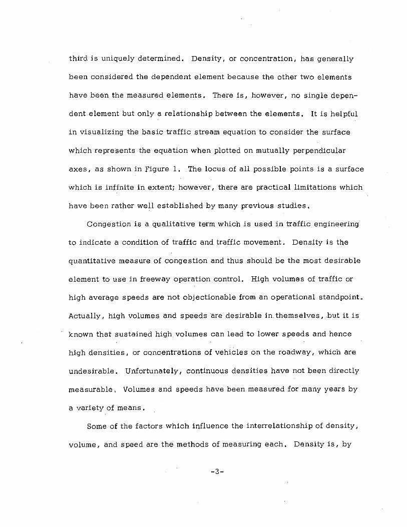
third is uniquely determined. Density, or concentration, has generally

been considered the dependent element because the other two elements

have been the measured elements. There is, however, no single depen­

dent element but only a relationship between the elements. It is helpful

in visualizing the basic traffic stream equation to consider the surface

which represents the equation when plotted on mutually perpendicular

axes, as shown in Figure 1. The locus of all possible points is a surface

which is infinite in extent; however 1 there are practical limitations which

have been rather well established by many previous studies.

Congestion is a qualitative term which is used in traffic engineering

to indicate a condition of traffic and traffic movement. Density is the

quantitative measure of congestion and thus should be the most desirable

element to use in freeway operation control. High volumes of traffic or

high average speeds are not objectionable from an operational standpoint.

Actually, high volumes and speeds are desirable in themselves I but it is

known that sustained high volumes can lead to lower speeds and hence

high densities 1 or concentrations of vehicles on the roadway, which are

undesirable. Unfortunately, continuous densities have not been directly

measurable. Volumes and speeds have been measured for many years by

a variety of means.

Some of the factors which influence the interrelationship of density 1

volume, and speed are the methods of measuring each. Density is, by

-3-

X (volume)

r I density)

... Q) Q. .. Q)

...------ INTERRELATIONSHIP SURFACE·

BOUNDARY

Figure 1. The Speed- Volume - Density Surface (One La~e)

-4-

y (speed)

its very nature, a space element of the traffic stream; volume is a time-

point (nonspatial) element; speeds are sometimes point elements (spo~

speeds or instantaneous speeds) or are sometimes based on travel times

over a finite, short distance (space mean speeds). Sensing devices have

been used to determine speeds and volumes at a point ( 1)* (or over a

very limited length of roadway) , and densities have been rapidly approxi-

mated at short time intervals, by electronic means, on the basis of such

point information. This process, in effect, extrapolates speed and

volume information obtained at a point to density over a distance of up

to a mile. Density fluctuates continuously and it becomes critically

high in certain spaces on a freeway in connection with the creation of

bottlenecks. Investigations at Texas A&M University by Keese, Pinnell,

and McCasland (2) have shown that traffic in the near vicinity of entrance

ramps becomes congested enough to reduce speeds as much as 50 per

cent or more during regular peak flow periods. From the fundamental 9 ":. 1:<-_,()_-

relationship: Volume is equalto density times speed,. 'it is obvious that

if a given volume of vehicles slows down, the density must increase,

resulting in more congestion.

It would be desirable to sense density directly over a given length

of roadway. From a control standpoint, it is hypothesized that density

* Numbers in pare:;-ttheses refer to references at th~~ end of the text.

-s.:.

sensing offers greater promise than the current methods of computing

density on the basis of speed and volume information.

If by some satisfactory means density were sensed, there would

remain the problem of determining the proper selected locations of

sensors, the required lengths of roadway to be sensed for density, and

the critical density values to be used for the controlled operation of

freeway traffic. It is necessary that the characteristics of density be

carefully studied by itself prior to its utilization as a control element.

Because density has been the dependent or calculated element heretofore,

little has been developed which would enable the study of the basic nature

of density.

SCOPE

This report includes parts of a general study of the various aspects

of vehicular density for use in the control of freeway traffic (3). Density

is herein considered singly as a possible control element of a freeway

operational system. This study provides information which may be useful

for freeway control methods. Electronic equipment manufacturers should

be encouraged by this study to develop density sensing systems.

The scope of this report specifically involves principal study areas

described as follows:

1. The principal features of existing methods used to measure or

estimate density are reviewed. There are two basic methods

-6-

involved. One is a process in which density is estimated on the

basis of speeds and volumes which are sensed at a point. The

other method, which is not yet operational, involves the actual

measurement of the density, or concentration of vehicles in a

space. The undesirable features and limitations of existing

equipment are listed, and the general features which are desirable

in density sensors are described.

2. Results of aerial photography studies of the Gulf Freeway in

Houston, Texas, are utilized to show how density may be related

to volume as well as to certain geometric features of the freeway

facility.

3. A field study method is described which yields continuous values

of vehicular concentration on certain sections of a freeway. The

results of several of these density-trap studies are analyzed for

the purpose of determining the variability and frequency distribu­

tions of freeway concentration and relating the length of sensing

sections to the variability of concentration.

4. The analysis of the data demonstrates a means of establishing

optimum, or critical, freeway concentration values and provides

a means of identifying critical, or bottleneck, sections at a free­

way which exhibit recurring high densities.

-7-

II

DENSITY SENSING EQUIPMENT

REVIEW OF CURRENT METHODS

There are presently several different firms which supply electronic

density computers. General Railway Signal Company of New York and

Automatic Signal Division of Connecticut have developed such systems.

Actually, the systems available at the present time are capable of

measuring both speeds and volumes; density is computed on the basis

of these values.

The computers utilized in density computations usually generate

analogue functions which may be recorded as analog data, displayed on

output meters, or used in connection with control systems. The input

information which is necessary for density computation by a computer

requires time to accumulate. The passage of a number of vehicles or

the time passage of several seconds or minutes is necessary in order

for the traffic stream to generate. data to be evaluated.

The electronic circuitry involved in existing traffic surveillance

analogue computers is beyond the scope of this study. It is possible,

according to some of the manufacturers, to modify or adjust the output

of such systems for a wide variety of purposes. A preselected time

period has been mentioned as a necessary constant for computing volumes

and average speeds. In many instances, manufacturers will offer several

-8-

different time intervals which may be used.

An altogether different type of density sensing is being developed

in England by the Road Research Laboratories. Charlesworth, Head of

the Traffic Section of the Laboratories, replied to this author• s inquiry

:=-:about the actual sensing of vehicles in a space, rather than computing

the concentration on the basis of speed and volume. In the reply, it

was stated that there had been a development of such a system which

11 measured the number of vehicles in the area adjacent to a large loop

detector. 11 It was stated that the detector produced an output depen­

dent upon the number of vehicles adjacent to its detector loop and has

been used to determine when the 11 level of traffic 11 in a traffic circle

exceeded a critical value. It was further stated that this instrument

would be commercially available in the 11 near future. 11

The detector loop referred to in connection with the instrumentation

in England is a known and utilized device in this country. Vehicle pres­

ence detectors which operate with loops installed just below the pavement .

surface are used at toll gates, traffic signals, etc.

These vehicle detectors, however, are used only to detect the

presence or absence of a single vehicle adjacent to (just above) the loop.

The output is a two-step function only, indicating an event is, or is not,

occurring. The development of the loop detectors to indicate the number

of vehicles adjacent to a large loop ( 1000 feet or more in perimeter) would

-9-

involve an analogue function output which would be indicative of the

number of vehicles. In this sense, the Road Research Laboratory is

developing a true density (or concentration) sensor rather than a density

computer.

PRESENT LIMITATIONS

The density (or occupancy) computers now available involve the

limitations of point sensing and time lag which are not actually limita­

tions of the density element, but are imposed by the means which are

now utilized in the computer-sensor scheme. As stated in the earlier

part of this chapter, density is not presently sensed by available equip­

ment; it is computed on the basis of volume and speeds, both of which

are time dependent elements of the traffic stream and must be measured

at a point on a facility. The information obtained at a point is then

extended such that, assuming unchanging conditions exist downstream

from the point, a density or concentration of vehicles is estimated on

the basis of a required r preselected time interval.

Density is a function of vehicles and roadway length only; time is

not a dimension of this element. Density exists continuously at all

instants in time. It is the one element which can be obtained at any

instant without counting for a predetermined time interval and thus would

be more readily available for control decisions.

Conditions do change from section to section along a freeway and

-10-

conditions at one point do not accurately predict or represent condi­

tions at all other adjacent points. Density is more nearly related to

congestion and it should be sensed directly in order to accurately

measure congestion. The devices now in use only predict, with limiting

assumptions, what the density might be downstream, and only then

after an arbitrary time period of counting.

It would seem that improved methods are forthcoming and that true

density sensing will be done in the future.

SOME DESIRABLE FEATURES

Economy is a feature to be desired in a density sensing device.

Methods are now possible which are too costly to consider. In order

to utilize density as an element of control information, it must be

economically feasible to sense it. A determination of the economic jus­

tification of density sensing or the benefit-cost ratio of traffic surveil­

lance systems is perhaps difficult at the present time. It is presumed

that in the developmental stages some research and traffic surveying

systems are not immediately economical but may result in long-term

savings in terms of lives, dollars , time, and information. It remains,

however, to develop an economical means of sensing density.

The systems developed should, of course, be density sensors (or

concentration sensors), and not concentration computers or estimators.

Such systems would desirably be highly reliable. As in any automated

-11-

device, it would be desirable to incorporate "fail safe" features or

positive indications when the system was out of order.

The scheme of operation of a density sensor should be such

that the failure of one component or sub-part would not create an

accumulative error in the output of the system~ Schemes involving a

continuous counting routine are typical of those which would accumu­

late an error if one counting element failed. More specifically, it

would be more desirable to feed the continuous output of a gridwork of

vehicle detectors into one total output such as that shown in Figure 2 .

than to periodically deduct the "out" detector sums from the "in"

detector sums in an arrangement similar to that shown in Figure 3.

The failure of one sensor in the gridwork scheme would cause a small

non-accumulative error in the output, whereas the failure of one sensor

in the scheme of counting 1 shown in Figure 3 1 would result in an ever­

increasing error as time progressed. An additional feature of the

desirable system shown in Figure 2 is that it requires no starting

technique. It would yield continuously 1 from the time the sensors were

activated, the concentration of vehicles within the section. The un­

desirable scheme shown in Figure 3 requires some special starting tech­

nique for the determination of the number of vehicles in the section at

the time the counting begins.

It would be highly desirable that the density sensors be unaffected by

-12-

IN

Figure 2. Desirable Summation Griawork of Sensors

OUT

Lane

Lane 2

Lane 3

Figure 3, Undesirable Scheme Utilizing Difference of Counting Sums

the speed of the vehicle. Some vehicle detector loops and radar

detectors will not operate if the vehicular speeds are below 5 miles per

hour. Detector loops may cease to detect the presence of a stopped

vehicle after a short period of time. The system would desirably sense

vehicles at high speeds as well as those which have stopped.

If vehicles could be sensed according to lanes, the system would

have more utility. It might also be desirable to let the influence of

large trucks be represented in the output of the system.

A system would desirably be durable and easily installed and

maintained. The utility of a density sensing device would be increased

if there was a wide range of roadway lengths which could be sensed.

In a very limited experimentation program undertaken at Arlington

State College, certain studies concerning the development of density

sensors were made. Attempts were made to utilize low frequency

electromagnetics which depend upon an electromagnetic field of a very

low frequency and a magnetic detection unit.. The poor isolation proper­

ties of the low frequency field resulted in unreliable detections because

the flux was not controlled, or confined, to a desired region. The use

of magnetometers was considered; however, a review of the cost of

such a system revealed that such a method would be too expensive to

investigate in this study. The method of sensing impedance shifts of

a transmission line placed along the center line of a lane was investiga­

ted and proved to offer promise in a revised application.

A system which appears to be feasible because of its economy,

reliability 1 and simple circuitry is one in which equally spaced, short

transmission lines are placed at right angles to the center line of a lane.

An oscillator supplies energy to the transmission line and a standing

wave pattern is set up adjacent to the line. Figure 4 illustrates the

relationship between the voltage and the distance along the line.

In the absence of any vehicle adjacent to the transmission line 1 a

-14-

voltage detector fixed at point A, Figure 4, would read some small

minimum voltage. The presence of a vehicle near the line causes a

shift in the standing wave pattern which would result in an increase

in voltage at point A. The direction of the wave shift is of no concern

because the wave pattern is symmetrical and a small shift in either

direction would result in the same voltage increase.

A schematic diagram of a transmission line circuit is shown in

Figure 5. The line itself is comprised of simply two ordinary parallel

wires. An oscillator is used which operates in the 100 megacycles per

second range and is rather inexpensive, costing about 2 0 dollars. The

rectifier serves as an envelope detector and the output voltage is

largely D. C.

Multiple detectors may be incorporated into a sensing system

similar to that shown in Figure 2. The voltage outputs of each detector

system can be combined to operate a voltmeter which could be cqlibrated

to read in vehicles rather than volts.

-15-

1

0

A

i\ 2

No C a r--___,

Distance Along a Transmisson Line-----_.

Figure 4. Standing Wave Variation Along a Transmission Line

t + Oscillator V (Output)·

Figure 5. Transmission Line Circuitry Scheme

-16-

III

AERIAL PHOTOGRAPHY STUDY METHODS

THE HOUSTON AERIAL PHOTOGRAPHY STUDY

In September I 1962 I aerial photography studies were made of a five

mile section on the Gulf Freeway (U. S. Highway 7 5) which extended from

the edge of the central business district in Houston southeastward to the

Reveille Interchange 1 where State Highways 22 5 and 36 intersect the

freeway. Two methods of aerial photography were incorporated in these

studies under the direction of the Texas Transportation Institute in cooper­

ation with the Texas Highway Department and the Bureau of Public Roads.

The two methods were the time-lapse and the continuous-strip.

There were two principal objectives of the aerial photography study

of the Gulf Freeway. It was de sired that the two aerial photographic

methods be compared for their applicability to aerial traffic surveys and

also considerable information concerning the operational characteristics

of the freeway was expected. The work was· contracted to two aerial

photography firms. Each firm utilized a Cessna 195 fixed wing aircraft.

Each company began flights at about 6:30a.m. and continued until about

8:00 a.m. and the two planes were required to be separated by at least

a two minute interval. The time-lapse plane was required to make nine

runs and the strip-film plane was required to make as many runs as pos­

sible and furthermore 1 was required to repeat its schedule of runs from

-17-

/

6:30a.m. until 8:00a.m. on a subsequent morning as soon thereafter

as practicable. This arrangement resulted in the nine time-lapse runs

and a total of twenty-two continuous strip-film runs. The planes were

requested to fly only one outbound run on the first filming day and the

strip-film plane was requested to repeat this procedure on its second

filming day.

During the filming runs, ground observers made volume counts at

several points along the five mile section of freeway. Several control

vehicles were specially marked on the roof and made runs in and out

continuously during the filming sequences for which they recorded

their travel times. No communication between the ground stations and

the airplanes was provided for. There was a synchronization of watches

one-half hour before the start of the filming flights.

Each of the twenty-two strip-film runs was developed and furnished

as positive film transparencies at a scale of about 1 inch to 300 feet. The

nine time-lapse film runs were developed and printed at a scale of 1 inch

to 100 feet. Figures 6 and 7 illustrate 1 to a reduced scale, these furnished

photographic types.

DATA REDUCTION

McCasland (4) 1 in reporting on the data reduction techniques used on

the Houston aerial photography study 1 emphasized that it was decided that

each method and each run would be subjected to as complete a reduction

-18-

-19-

-20-

of data as possible. Had it been desired only to analyze the films for

a particular characteristic I such as density, the total time involved

could have been reduced.. The basic reduction of the film data was com­

pleted in the spring of 1963 and was in a general form on punched cards

which could be utilized for many different types of analysis.

DENSITY-VOLUME RELATIONSHIP

Since it is the volume which ideally should be kept as high as

practically possible 1 the relationship between volume and density

should be well established if density is to be used as a control ele­

ment. Each freeway may exhibit a different characteristic volume­

density relationship. It is furthermore likely that different sections

along a freeway will have their particular volume-density characteris­

tics. Factors which can influence this relationship are not only the

geometric features of the freeway such as lane widths, grades 1 median

widths 1 shoulder widths I curvature 1 sight distance 1 entrance and exit

ramps I etc. I but also the posted speed limits I size ·Of the metropolitan

area I and distance from the central business district I etc.

Any specific section of a particular freeway facility can be studied

for the volume-density relationship. The continuous strip aerial photog­

raphy described earlier was utilized to make a study of this type. A

test section was selected such that no entrance or exit was possible

within the section 1 but all vehicles entering at one end exited at the

-21-

other end or stopped within the section.

The number of vehicles within the test section was obtained for each

of the 22 different flights. The speeds of the vehicles were averaged

(space mean speeds) and the volumes were then computed on the basis

of the density and the speeds. Table l is a tabulation of the 22 runs.

The 22 points obtained in this study are plotted in Figure 8, which

shows the volume-density relationship for this particular study section.

A curvilinear regression, using a second degree parabolic relationship,

yielded the equation of best fit:

v = 7 5 D - 0 • 2 0 5 D2 - 8 12 I

in which V = Three-lane volume (veh/hr).

and D = Three-lane density (veh/mi).

Thi.s regression analysis placed no restrictions on the constant term 1

thus a when the density in this equation is zero, the volume is -812.

The true relationship is such that volume is zero when density is zero.

The equation, however, is the best second degree curve fit for the points

shown, all of which are in the volume range of 2500 to 6500 vehicles per

hour.

The volumes as predicted by the equation were computed for each of

the 22 densities obtained in this study and plotted versus the volumes,

obtained in the study u as shown in Figure 9. The coefficient of correla­

tion for these points is 0. 9 06 and R-square is 0. 82 1 or it could be said

that the second degree equation accounts for about 82 percent of the

-22-

TABLE 1

Continuous Strip Aerial Photography Density Study Tabulation

Vehicular Concentration (per 2000 ft)

Space Lane Lane Lane Mean

Run 1 2 3 Total Density Speed Volume

1 4 5 8 17 44.9 53.6 2407 2 7 10 9 26 68.6 38.3 2627 3 9 11 6 26 68.6 51.5 3533 4 8 10 11 29 76.6 50.5 3868 5 14 22 18 54 142.6 46.9 6688 6 13 18 14 45 118.8 43.3 5144 7 11 19 18 48 126.7 43.0 5448 8 15 24 17 56 147.8 41.7 6163 9 14 21 20 55 145.2 38.6 5605

10 12 14 15 41 108.2 45.1 4880 11 9 11 15 35 92.4 49.1 4537 12 8 14 12 34 89.8 48.7 4373 13 9 14 10 33 87.1 50.2 4372 14 9 14 11 34 89.8 52.9 4750 15 10 15 13 38 100.3 47.1 4724 16 15 20 17 52 13 7. 3 43.1 5918 17 14 21 23 58 153 .. 1 33.2 5083 18 12 20 15 47 124.1 40.2 4989 19 13 14 15 42 110.9 39.8 4414 20 16 18 19 53 139.9 40.8 5708 21 15 20 19 54 142.6 43.2 6160 22 15 19 18 52 137.3 40.9 5616

-23-

..: J:

""':-..s::. 41

~ 41 E ;:)

0 >

41 c 0 _, I 41 41 ...

..s::. 1-

7000

6000

5000

.4000

3000

2000

1000

0 0

I 1/

~~~~ :.-

~ ;"" ......

... k

I-AI

1/11 I'"' &/

[J • I?

1/ v •

l% t- ~= 7 D 0 2( 5[ 2_ 812

1/

50 100 150 200

Three-lane Density (Veh.jMi.)

Figure 8. Volume-Density Relationship Obtained from Continuous Strip Aerial Photography

-24-

..... J: 7000 ':-..c.

Q)

> 6000 Q)

E ::;)

5000 0 >

Q)

r:: 4000 0 _, I

Q) Q) 3000 .....

..c. 1-

"'tl 2000 e Q)

0 E 1000 -"' w

1000 2000 3000 4000 5000 6000 7000

Actual Three-Lane Volume (Veh:/Hr.)

Figlire 9. Estimated Volume Versus Actual Volumes Obtained in the Continuous

Strip Aerial Photography Study

-25-

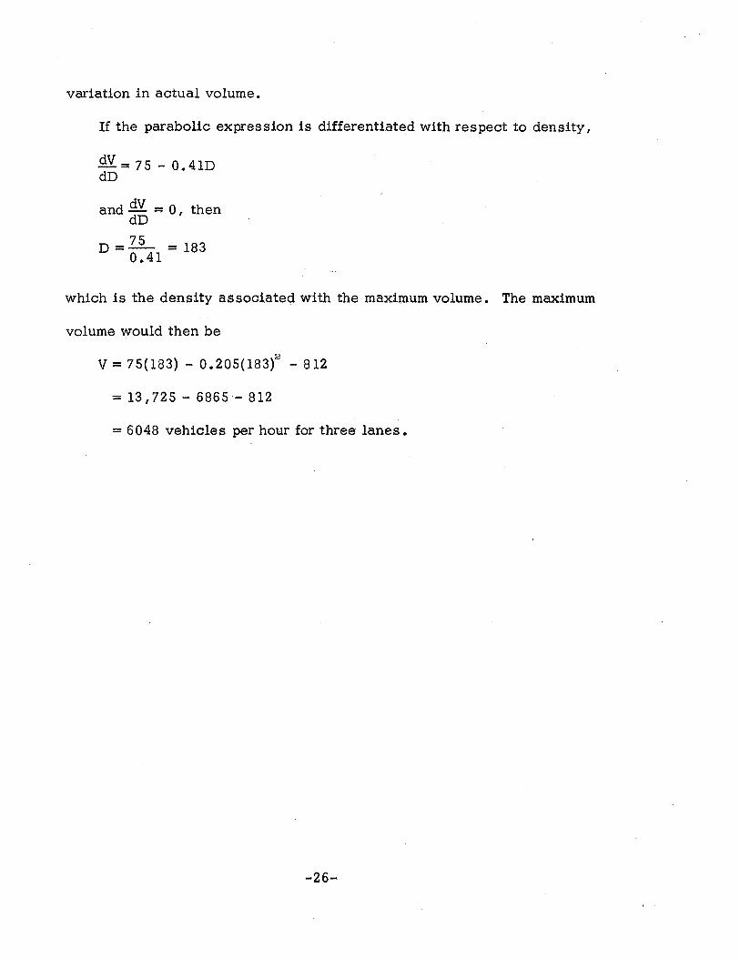
variation in actual volume.

If the parabolic expression is differentiated with respect to density,

dV = 75- 0.41D dD

and dV ::; 0, then dD

D =.z.L = 183 0.41

which is the density associated with the maximum volume. The maximum

volume would then be

v = 75(183)- 0.205(183)2

- 812

= 131725- 6865- 812

= 6048 vehicles per hour for three lanes.

-26-

IV

DENSITY TRAP STUDY METHOD

GENERAL CONCEPTS

In veiw of the expense of aerial photography methods of studying

freeway traffic flow characteristics and because only a few instan­

taneous states of density were available from such studies 1 it was

necessary that another study procedure be developed which would pro­

vide more 1 and preferably continuous 1 density information. Economy

and mobility were important factors in the development of this procedure.

It is emphasized that the study method which was developed was not

basically a method to be developed for automatic density sensing; some

desirable features of automatic density sensing are discus sed in Part II.

This procedure involved a means of obtaining a continuous record from

which actual densities 1 or more correctly 1 vehicular concentrations

within a section of the freeway were derived after a data reduction of

the record.

The density trap involves a selected length or section of roadway.

The upstream end of the lanes of one-direction traffic constitutes the

beginning of the trap or the "in" point. The downstream end of the

section is the end or "out" point. Vehicles are counted in and out of

the section or trap. The simplest case is that which involves no entrance

or exit points within the trap. The number of vehicles I k I in the trap at

-27-

any time, t, can be expressed

t t k = k0 + ~ I(T) - :E O(T)

T=to T=to

where k0 is the number of vehicles in the trap at some beginning time,

t 0 , I(T) is the number of vehicles passing in as a function of time and

O(T) is the number of vehicles passing out as a function of time.

Several practical problems exist when attempts are ma:l e to put

this principle into actual use. First, the vehicles must be counted

very accurately because any error made in counting will be thereafter

reflected in the concentration, k. Second, since the number of vehicles

passing in and out have the same time base, there should be no error

in synchronization of the beginning time or lapsed time after beginning.

Third, the number of vehicles 1 k0 in the trap at a beginning time, t0

, is

not readily determinable. Finally, the record of such values as k, I(T) ,

and O(T) is continuously changing in time and requires some dependable

recording scheme.

METHOD DESCRIPTION

It was decided, as a matter of expediency, that the vehicles would

be counted manually. Adequate numbers of personnel were available who

had experience in counting traffic and it was felt that automatic vehicle

counters were not economically justified. The installation of the counters

would have also been time consuming and would not have had the mobility

-28-

of human observers. ·It was realized that a method of checking would have

to be developed regardless of whether automatic or manual counters were

used.

In order to obtain a common time base and properly synchronize all in

and out counts, it was decided that each observer 1 or traffic counter 1 would

operate an electrical switch which was wired to an electrical counter mounted

on a centrally located counter board. All counters for both the 11 in 11 and "out"

points were mounted on the same counter board, thus could be observed

simultaneously at any instant in time. Figure 10 shows a wiring scheme

for the density trap method.

In order to accurately ascertain the number of vehicles 1 k0 , in the

trap at some beginning time, t0 1 a span of pace cars were required to

maneuver such that they were abreast of each other when traveling through

IN POINT

Common Ground

Counter Board

Common Ground

Figure 10. Wiring Scheme for Density Trap Apparatus

-29-

OUT POINT

the trap thus preventing any vehicles from passing them or their passing

any vehicles.

The pace cars were the first cars counted by every observer 1 thus 1

when the out points began counting 1 the difference between the total in

and the total out was the actual concentration of vehicles within the trap.

A check on the accuracy of the counting was pro~tded by having the

pace cars pass through the section a second time to end the count. The

pace cars passed through the section abreast and were the last vehicles

counted by every observer. The final totals of the vehicles in and the

vehicles out were identical if no mistakes had been made in counting.

The recording of the data was accomplished by photographing the

counter board with a 16 mm. moving picture camera at a rate of 10 frames

per second. This system provided a continuous record of the density

trap studies I each of which lasted from about 6 to 18 minutes. The

reaction time of the observers was found to vary about 0.2 second.

Several observers were required to actuate their counting switches for the

same vehicles passing a given point in order to determine this variation.

This variation in counting could have been overcome by using automatic

vehicle counters; however, for the purposes of this study of vehicular

densities 1 manual counting was considered sufficiently accurate. The

camera speed of 10 frames per second was deemed sufficiently fast con­

sistent with the variation in manual counting accuracy.

-30-

The counters were flush-mounted on a small plywood board which

comprised the face of a folding leg frame. An electric clock from an

automobile was mounted on the face of the panel and was operated by a

12 volt dry cell battery. The clock provided a record of the time of day

and, by observing the second hand I an accurate check was made of the

number of frames per second taken by the moving picture camera. The

camera was equipped with a 1200 foot film magazine and an electric drive.

The power for the camera drive motor was provided by a portable I gasoline­

powered generator. Figure 11 shows the camera in position for filming the

counter board during a study at the Gulf Freeway in Houston.

Radio communication between the pace car drivers I the filming station

Figure 11. Filming Station for Density frap Study

-31-

and the counter stations was provided. Ideally, there would be a total

of four transceivers for such a study; one in a pace car, one at each

counting station, and one at the filming station. Each transmitter

should have a range of several miles in order to insure communication

with the pace car which might be required to travel considerable distances

from the trap section. Field telephones could be utilized between the

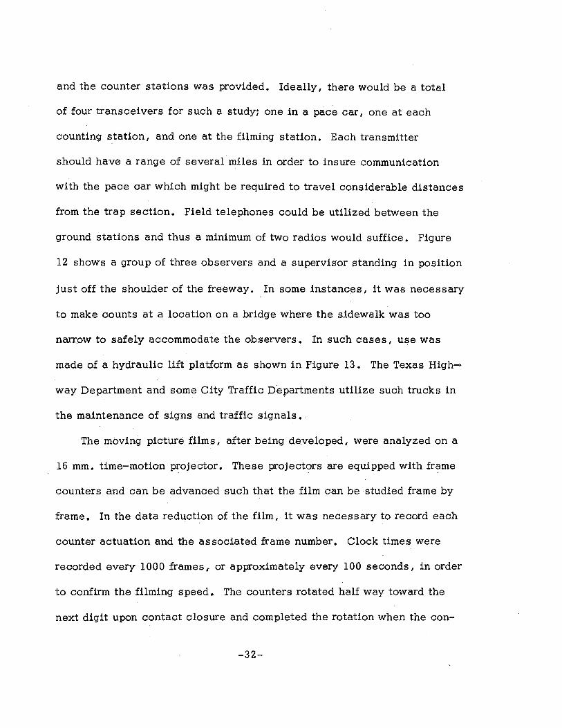
ground stations and thus a minimum of two radios would suffice. Figure

12 shows a group of three observers and a supervisor standing in position

just off the shoulder of the freeway. In some instances, it was necessary

to make counts at a location on a bridge where the sidewalk was too

narrow to safely accommodate the observers. In such cases, use was

made of a hydraulic lift platform as shown in Figure 13. The Texas High._

way Department and some City Traffic Departments utilize such trucks in

the maintenance of signs and traffic signals.

The moving picture films, after being developed, were analyzed on a

16 mm. time-motion projector .. These projectors are equipped with frame

counters and can be advanced such that the film can be studied frame by

frame. In the data reduction of the film, it was necessary to record each

counter actuation and the associated frame number. Clock times were

recorded every 1000 frames, or approximately every 100 seconds, in order

to confirm the filming speed. The counters rotated half way toward the

next digit upon contact closure and completed the rotation when the con-

-32-

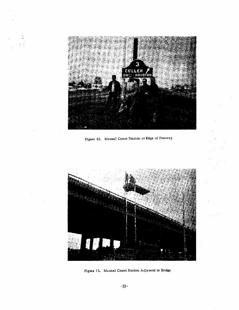
Figure 12. Manual Count Station at Edge of Freeway,

Figure 13. Manual Count Station Adjacent to Bridge

-33-

tact was broken. Attention was given to recording the precise frame

number of the initial contact closure.

An added feature of the density trap method was incorporated

during the studies made in early 1964 in order to obtain the travel times

of several vehicles through the trap section. Two additional counters

were used for this purpose and were also mounted on the counter board.

Additional circuits with switches were provided similar to the counting

circuits for each of the two additional counters. The observers using

these counters were stationed at each end of the trap section near the

volume count observers and were provided with communication with one

another. Either field telephones or portable radios could be used for

this purpose. The observer stationed at the in point selected a 11 floating 11

vehicle and actuated his switch when the vehicle entered the trap section.

He then described the vehicle to the other observer at the out point, who,

in turnr actuated his counter when the described vehicle exited the trap.

The filmed record of these two counters provided sufficient information

to calculate the speeds of these vehicles through the trap.

It should be pointed out that the trip times through the trap were not

necessary, but were obtained as a possible source of verification of

speeds calculated from the volume and density information obtained in

the study.

A total of six density trap study runs were made in Houston on

-34-

Wednesday morning, November 27, 1963. The study site was selected

on the Gulf Freeway in the region of Station Number 100. The inbound

lanes of the facility have no entrance or exit ramps for a distance of

about 1800 feet at this particular location ·(see Figures 6 and 7). The

out-count station was set up at Station 86 + 50 and the in-count stations

were set up at three different points in order to vary the trap length. In­

point stations at 92 + 30, 95 + 40, and 102 + 80 provided trap lengths of

580 feet, 890 feet and 1630 feet respectively. Personnel from the Texas

Transportation Institute and the Texas Highway Department were utilized

in making the Houston studies. Table 2 lists the run numbers and lengths

of trap sections and also shows the difference in the final in and out counts

obtained. Only runs 1, 4 1 and 5, which tallied exactly, were reduced

frame by frame for complete analysis. The film reduction, frame by frame,

required two persons about 42 hours of moving projector time and about 84

man-hours.

No serious conge_stion occurred during any of the six study runs._

Information concerning volumes of traffic associated with high densities

was desired.

A new study site for congested conditions was sought which would

provide vantage points for observers from which they could make accurate

counts without calling attention to themselves. The North Central Express­

way in Dallas is. a partly depressed facility 1 that is, it passes under many

-35-

TABLE 2

Summary of Density Trap Study Method Ruris in Houston

Run Time Run Trap Total Total Count No. . (A.M.) Duration Length Vehicles In Vehicles Out Error

1 7:40 15 min 580 1 1268 1268 0

2 8:30 12 min 890' 749 746 3

3 9:15 12 min 1630 1 476 477 1

4 10:45 12 min 1630• 499 499 0

5 11:10 11 min 890 1 466 466 0

6 11:40 11 min sao• 419 421 2

of the major streets. The embankments in the regions of overpassing

major streets or the overpassing structures themselves provide positions

from which observers can accurately count traffic from less obvious

positions. At the Haskell Street overpass, the North Central Express-

way provides a section about 1200 feet in length with no entrance or

exit ramps. This section of Expressway was observed to congest rather

heavily each day on the outbound lanes during the P.M .. peak. On Friday

afternoon, February 7, 1964, personnel from the Texas Transportation

Institute and Arlington State College made a study at the Haskell Street

location on the North Central Expressway. The study involved two runs,

hereafter referred to as runs 7 and 8. Run 8 involved a difference of 9

-36-

vehicles in the in and out count and was not analyzed frame by frame.

Run 7 was made at about 5:00 p .. m. and had a duration of six minutes.

The trap length was 900 feet and the total vehicles counted was 459, at

both the in and out stations.

-37-

v

ANALYSIS OF DENSI1Y DATA

DENSI1Y DATA CONCEPT

Volume, when reduced to its most elemental form based on time

gaps between successive vehicles, is quite widely variable. Of course,

when longer periods of time are used to count more than two vehicles,

the variability is reduced. In the density trap study method, the volume

in and the volume out of a particular section might be represented as

shown in Figure 14. Although the shortest-term volume rates in and out

may be quite variable, the density of vehicles within the section will be

less variable if there is an average of over two vehicles in the trap. The

volume out is not independent of the volume in. If an average travel

time through the trap were ~t, there would be similarity between the two

volumes if the origin of the. volume were shifted an amount equal to t.t.

c:

Gl -0

"' Gl

E ~

0 >

TIME

-~ 0 Gl -0

"' Gl

Trap Section ;

I • I c; Ave rage Travel

Time=~ t

>

Figure 14. Volume Rates In and Out ot a JJensity Trap

-38-

TIME

As the trap length increases, this similarity between volumes tends to

diminish. The longer the trap length, the less variable the density will

be. This is comparable to a longer counting period for volumes entering

(and leaving).

DENSITY-VOLUME RELATIONSHIP

The density trap study method provided considerable data suitable

for establishing the relationship between density and volume. The

approach in this analysis involved the assumption that a short-term

rate of flow-in immediately preceding any specific concentration should

be compared to that concentration. Furthermore, the short-term rate of

flow-out immediately succeeding any particular concentration was com­

pared to that concentration. The basis for this concept is illustrated in

Figure 14. The time involved in the rates of flow were based on the

approximate average travel time through the trap. The average travel

times through the trap were either measured, as described earlier, or

obtained from the Ume required for the pace cards to traverse the trap

at the beginning and end of any run. Since a rate of flow was being

computed which involved dividing the number of vehicles observed during

the time period by that time period, the precise time interval to be used

was not of absolute importance as long as the time interval was generally

about the average travel time for the trap. The time intervals used for

the various runs analyzed are shown in Table 3.

-39-

Run No.

1

4

5

7

TABLE 3

Density Trap Study Method Travel Time And Space Mean Speed Tabulation

Average Travel Time Hrs.

0.00300

0.00680

0.00357

0.01070

Average Speed (Mi./Hr.)

36.6

45.4

47.2

15.9

A computer program was written to determine the rates of flow in and

out for each concentration obtained in runs 1$ 4$ 5, and 7 and the rates of

flow were extended to volumes, in vehicles per hour, and the concentra-

tions were expanded to density, in vehicles per mile. A curvilinear

regression involving a second degree parabola resulted in the equation

V = 65.5D- 0.179D2 - 80

Only every twentieth value of density and the corres pending value of

volume is shown in Figure 15. The large number of obtained points renders . .

plotting every point impractical.

When this expression is solved for the maximum volume, by differen­

dv tiating and setting dD = 0, the maximum volume is 5930 vehicles per hour

for three lanes and the optimum density associated with this maximum volume

is 183 vehicles per mile for three lanes.

dv The differential of this equation, dD = 65.5 - 0. 3 58D, represents the

-40-

8 =Run No.1 • = Run No.5

• =Run No.4 • = Run No.7

7000 f)

1 ..

6000

... :::t: 5000

I "'-..

.j:>. .i. ....... I ~

Q)

4000

E ::::>

0 > 3000 Q) 1: 0 ....

f) ·s & (t

~v ~[ ~ Pi: 2_ . ~ ~ ,_..

j :Iii ' -....... I=~ 5. o. 80 e ~ r-.....

~ ft (j) lt8 e " •V e e e e e .......

~ . . v . . . ·f' liM Q . . . . . 'I\.

ek' le p

" W..! ~~·

" I 2000 Q) Q) ... If."

..r: 1-

"' lf

1000 li 0 ll

0 50 100 150 200 250 300 350 400

Three-lane Density (Veh/Mi.)

Figure 15, Volume-Density Relationship Obtained From Density Trap Stmlles

slope of the volume-density curve at any point and when density is

zero, the slope is 6 5. 5. The slope at zero density is what might be

termed the 11 free flowing 11 speed of the section of freeway since the

slope is volume, in miles per hour divided by density, in vehicles

per mile which is equal to the space mean speed in miles per hour. To

be completely correct, the curve should pass through the origin; however,

this curve comes considerably closer to the origin than the one developed

in the continuous strip aerial photography study.

The true shape of the volume-density curve past the maximum volume

point is difficult to ascertain. The volumes associated with extremely

congested traffic conditions are known to be quite small and the density

reaches its maximum value when the stream of vehicles has been halted

in a 11 bumper to bumper 11 stoppage. For the purposes of this study, it is

not necessary to determine this branch of the curve; the maximum volume

and its associated density is the limit of importance in using density as

an element of control. ·It is believed that the density trap method, however,

might be a useful study procedure for determining the congested, or right,

branch of this curve.

THE VARIABIUTY OF CONCENTRATION

Although density is, by current usage, defined as the number of

vehicles in a one-mile length of roadway, concentration is taken to mean

the number of vehicles in a length of roadway less than a mile long. The

-42-

two important factors affecting the variability of concentration are the

length of section involved and the volume of traffic.

A simulation of freeway traffic with an IBM 709 digital computer (3)

indicated that distributions of concentrations could be approximated

rather closely by the Poisson distribution, particularly for light to medium

volumes of traffic. This simulation indicated that the mean concentration

was directly proportional to the length of section involved for any given

volume. The simulation furthermore indicated that the variability of con-

centration was inversely proportional to the length of section involved for

any given volume. Specifically, the standard deviation of concentrations

was related to the length of section by the following relationship:

cr , where cr is the standard deviation of the concentrations a 1

observed in a length of section 1 1 , and era is the standard deviation of

the concentrations observed in a length of section La • The lengths of

sections investigated ranged from 500 feet to 2000 feet.

The standard deviations were observed in the simulation program to

be a function of volume, however, for a section length of 1000 feet, cr

ranged between 3 and 4 vehicles for all volumes. The actual validity of

these simulated variations was established rather well by the field studies.

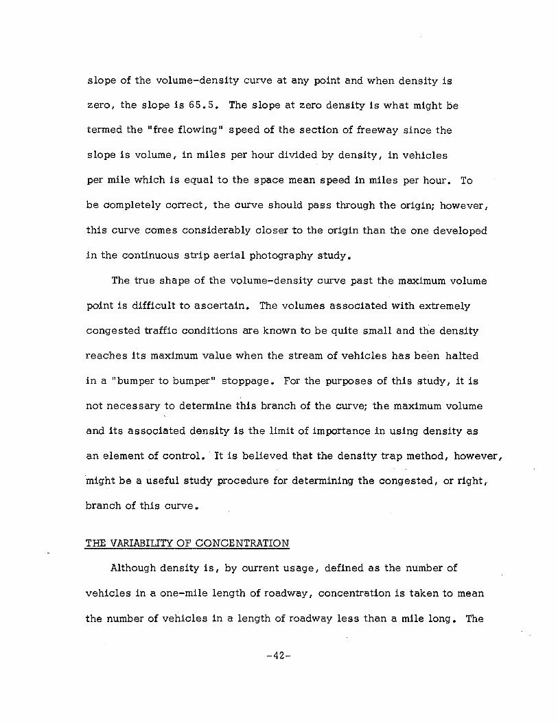
The frequency distributions of concentrations obtained from the

density trap field studies were calculated on a time basis. The frequency,

in other words, refers to that portion of the time that a particular concen-

-43-

tration was observed. Figure 16 shows the frequency distributions for

runs 1, 4, 5, and 7, and the Poisson distribution with the same mean

value is superimposed on each plot. Runs 4 and 5, as previously stated,

involved moderate to light volumes of traffic and it is seen that the

concentration distributions are quite similar to Poisson distributions. The

standard deviations of these two runs are approximately equal to the

square root of the mean, which would be the case for a Poisson distribu­

tion. Run 1 involved high volume flow, or generally optimum volume of

flow. The distribution of density for this ru;n is observed to be significantly

less variable than the corresponding Poisson distribution. Run 7 involved

congested flow conditions with volumes less than optimum. The standard

deviation obtained in this run was considerably less than would have been

obtained with a Poisson distribution.

It should be pointed out that there was no control of volume in these

field studies and only the lengths of traps were varied. The durations of

the runs were comparatively short, however, and it is unlikely that a

general change in the volume occurred during any specific run. The

lengths of the traps had an obvious effect on the mean value of concen­

tration for any similar volume conditions. For example, the mean concen­

tration value, considering moderate to light volumes of traffic, of a trap

length of 1630 feet in run 4 was 15.67 vehicles as compared to a mean of

8. 72 in a trap length of 890 feet in run 5. The standard deviation of the

-44-

..... lliliilliliilii&iiiilliill!lll liili.iiiiiiillliiliillllillllililliiil. .20

>-

g () z .IS w

"' ::J ::J 0 0 -w 1.1.1 .• 10. a::: .10

a::: u.. ..... w lolA > > ~ .OS -- <( s -1

w I a::: ... 00 I 20

30 ___ 11_0 so 60 IJ 30 Ml. * ~Q. 70 10 ll

CONCENTRATION ll CONCENTRATION

I

&; I

..20..i.ll I I I I 1.11.11 1..1._0 Lt"l..ilLI 0..1 II I ill I I I I 1.1 I Ill I 1·1 I I I I I I I I I I I I I I Ill I I I I I I I II .20

>i >-u u z J5 z .15 w w ::J ::J 0 0 w w a:: JO a::: .10 .... _u.. ~ w > > ...... .D5

..., .OS 1-c( <t

--1 -1 L&.t w .0::, a::: .o .o

401 60 70 0 10 .20 30 110_ so 60 70 0 10 20 30 50

ll ll CONCENTRATION CONCENTRATION

Figure 16. Concentration Distributions Obtained From Density Trap Studies

concentrations in run 4 was approxim'ately equal to the square root of the

ratio of the trap length used in run 4 to the tr~p length used in run 5 times

the standard deviation of concentrations in run 5, or

This would appear to be a fairly reliable relationship between the lengths

of sections involved and the variability of concentrations for light and

medium volumes. For the greatest volumes as well as for the congested

flow conditions, the variability of concentration was observed to be con-

siderably less than for the light to moderate volumes. It might be pointed

out, however, that for runs 1 and 7 the relationship

did happen to be very nearly correct.

The standard deviations obtained in these four.field studies were all

calculated for an arbitrary trap length of 1000 feet by us.ing the relationship

Table 4 lists these values along with the approximate volumes. The values

in these studies indicate that the standard deviation of concentrations ob-

served in a 1000 foot section of three lanes of freeway will be about three

for high volume flow and also for congestedlower volumes and, for light to

moderate traffic flow conditions, will be about four. Stated another way, it

-46-

can be said that the standard deviation of concentrations observed in a

1000 foot section was found to be about four for lower concentrations and

three or less for medium to high concentrations.

TABLE 4

Standard Deviations Obtained in Density Trap Studies

Run Number

1

4

5

7

am

2.24

4.73

3.79

2.78

a 1000

2.94

3.71

3.94

2.88

-47-

Approximate Volume

5050

2550

2650

4300

VI

SELECTION OF LENGTHS AND LOCATIONS FOR DENSITY SENSING

LOCATIONS OF CRITICAL OR BOTTLENECK SECTIONS

Aerial photogrammetry studies of traffic flow characteristics have

been analyzed for density contours by May, Athol, Parker 1 and Rudden ( 5) •

In such an analysis, the concentrations of vehicles along the roadway are

obtained for successive short time intervals of about five minutes. A con­

tour is obtained by plotting the densities on a chart with the station num­

bering (100 foot stations) as an abscissa and time of day as ordinate.

Studies made during peak traffic flow periods will show the position, or

station numbering I of high density locations and the time of day the high

densities exist. The duration of high density, or congested conditions,

can be determined by noting the vertical height (time) of any particular

density contour at a particular location along the freeway. If studies

made on several different days have similar locations of high density con­

ditions 1 it is .reasonably certain that the particular locations· are critical

or bottleneck sections.

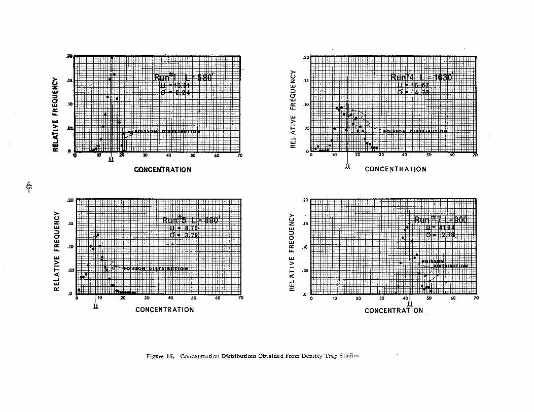
The aerial photogrammetry studies made on the Gulf Freeway in the

fall of 19 62 were analyzed for the purpose of plotting density contours.

Drew ( 6) has shown that the morning peak flow toward the city of Houston

results in several locations of high density flow. Figure 17 shows the

results of the three-lane density contour for the Gulf Freeway~ from 6:45 to

-48-

I. & G.N. RR SCOTT ST. CULLEN H.B.&T. RR DUMBLE H.B.& T. RR TELEPHONE

~1.40_........... "----~ .......... r-._ .......

~ 7;35 ( ) - '-- ~ ~

....... ~

/ --...... _,.) - 7:25 ~ ·-- v "-

........... 1.40 ........... <::'" I--,.. ...---& 7:15 .... ~

';/ ....._1~ ~1.40 -- ....... - /"' 140

0 7:05 v100 • - "':;>- -= 1::1.40-.~ 6:55

(""' 100 ..... I

~ Station20 30 40 50 60 70 80 90 100 110 120 130 140 150 I

\AYSIDE BRAYS BAYOU GRIGGS~[ WOOlRIDGE REVEl~ r~ l

~ ....... /

' / .......... \ ......... / 1\ )p--- ~~~l~ \ \

I "' {I\. I 4~ \ 1-.:35 ~ ""' ~ \

""' 7:25 '-... ~2.40-~ -- - ......._ r-..__ t--360 t-- - -·.· ·- "'"'"' -- 7:15 --- ~~ ---;::. ~ (_ L-240 ~----- 1:os 1--1-140- -.. - '-

!'----::> t-. 1 tsU' ::.:::::: ~ - 6:55 ·ltv\. ~6'0~ ........ v

f.-..-:-':" ~

160 ___ 17j) ____ ____1!_0 190 200 210 220 ~ 230 240 250 260 270 2·80 290 300

Figure 17. Density Contours (Three-Lane Total)

7:45a.m. A line sketch of the freeway, frontage roads, entr~nce ramps,

and exit ramps is shown above the contours.

It can be seen that in the region of Station 285 + 00 extremely high

densities did occur. A three-lane density of over 420 vehicles per mile

corresponds to almost a complete stoppage of vehicles, or, at best, a

stop-and-go or crawling-speed condition. The merging of two state

highways with the Gulf Freeway at this location presents a serious problem

on the facility. Subsequent studies made on the Gulf Freeway indicate that

the critical sections shown on this density contour generally tend to appear

at the same locations more or less regularly.

This study procedure appears to provide a u.seful basis for the selection

of density sensing locations. The contours also seem to indicate that

lengths of 1000 feet or less might suffice for density sensing trap lengths.

CONSIDERATIONS OF DENSI'IY SENSING SECTION LENGTHS

The volume-density relationship obtained from field studies of a

section of the Gulf Freeway indicated that the density associated with

the maximum flow rate was about 180 vehicles per mile for three lanes.

The concentration in a section 1000 feet long corresponding to this optimum

density would be about 34 vehicles. The variability of concentration in

a 1000 foot section indicated that the standard deviation of concentration

would be about three vehicles for moderately heavy or heavy volumes and

that the distribution of concentrations would be approximately normal. A

-50-

standard deviation which is only 9 percent of the mean concentration

indicates the high degree of reliability which is inherent in sensing

concentration (or density), and, as it has been pointed out, this sensing

can be continuous thus affording instantaneous indications of the traffic

flow condition.

It may not be economically feasible or even necessary to sense

density continuously along a freeway facility. A density contour analysis

would seem to provide a basis for the selection of sections to be sensed.

There is an indication that the standard deviation of the concentration, for

any specific volume of traffic, is related to the length of section being

sensed by the equation

As the length of a sensing section increases, the concentration of

vehicles increases proportionally. The standard deviation increases

proportional to the square root of the section length, thus, the ratio of

the standard deviation to the mean decreases as the length of section

increases. Figure 18 shows this relationship. It would appear that

little increase in confidence would result from sections longer than 1500

feet and that acceptable sensing reliability may be possible with sections

as short as 500 feet.

-51-

J, N

I

0 S2 )(

\)I~

I --+ r ..... l i--! _, I

20~-----Ll-~~~~~~~~~~~~-r~~~~--j·--·--,---t---'---:----+--+-

~~-J ______ J --- -----··-··-f·----·+· . I

;

·---t--~- - -- . ! -· .;...-. --~ . .. -+

15.-~~----~~------~------~-r-+~-+~-4----~--~----~~--~~--

---.-+--" ;\ ____ ·----f-;.. --+---·-I

. ·-·-·- ----+- .. -----4-- ..... ___ -----· --·----+----·

···--r--~------- -;------. .;..- .................. ---f..-

10~~----~--~---+--~~~-+~~~-+------L~~~~-+~~

---·---- -------··----+--

5 I

t i j .. ···--;-----+ --~---·-··-t

. I 1-----~-- ............... t-----t

300 600 900 1200 1500 1800 Length Of Section

Figure 18. Relationship Between the Standard Deviation Percent of the Mean Concentration and the

Length of Sensing Section at High Volumes

VII

CONCLUSIONS AND RECOMMENDATIONS

This study of vehicular density has singled out the one element of the

traffic stream which, because of the difficulty of measuring it directly,

has been largely relegated to be the dependent variable in the expression

q = k v. By a focused attention upon this element, this study offers these

conclusions, subject to the recommendations which follow.

CONCLUSIONS

1. Density, or concentration, is an independent element of the traffic

stream which is subject to direct measurement, feasible to sense directly

and is most directly related to the congestion of traffic. The q-k-v sur­

face, as shown in Figure 1, is a useful concept in considerfng the rela­

tionship between speed, volume, and density.

2. Reasonably close agreement was found between the maximum or optimum

density and theoretical optimum densities. It is possible, with field studies,

to establish the optimum density, associated with a maximum volume, for-·

particular sections of a freeway, and these optimum densities may not be

the same for all sections along a freeway.

3. Frequency distributions of densities were found to be closely approxi­

mated by the Poisson distribution, or a random spacing of the vehicles, for

light and medium volume conditions, or uncongested conditions; the distri­

bution of densities was found to be considerably less variable, however,

-53-

for heavy volume or congested flow conditions. These relationships

agree with several theoretical considerations of traffic flow.

4. The mean concentration of vehicles within a section was a function

of volume which was approximated rather well by a parabolic relationship

for the light traffic volumes up through the maximum volumes of flow.

5. The mean concentration was also proportional to the length of the

section considered.

6. The variance of the concentrations was approximately proportional tC>

the length of the section involved. Thus I the standard deviation was

approximately proportional to the square root of the section length. For

any particular volume 1 an increase in section length will result in a

standard deviation of concentration which is a smaller percentage of

the mean concentration.

7. Density sensing systems can offer the unique advantage of having

continuous and instantaneous values for use in the control of freeway

traffic systems and will not depend upon some time interval for counting

and averaging before a new output is available for control purposes.

8. It is possible to develop a density sensing system utilizing high

frequency 1 transmission-line type sensors which make use of voltage shifts

caused by vehicles adjacent to the sensors.

9 • Aerial photography methods of studying traffic characteristics can be

utilized to determine volume-density relationships; such methods are use-

-54-

ful in obtaining the density contours for a facility. The density contours

can be used to identify the regular bottleneck sections which recur daily.

10. The density trap method of study offers advantages in studying the

continuously variable nature of density and the relationship between den­

sity and speed and volume ..

RECOMMENDATIONS

An actual density sensing system needs to be developed ai).d produced

for evaluation. Such a system should have a continuous output proportional

to the sum of the vehicles in the section at any instant and should not be

based on the result of a subtraction process or data processing which sub­

tracts a downstream count from an upstream count. A proper system would

not involve a cumulative I or increasing error if a particular sensor in the

system failed 1 but would continue to give an output in error only by the

amount attributed to the faulty sensor ..

A density sensing system which has been properly evaluated should be

installed at a section or sections on a freeway which have been previously·

selected as critical locations by the density contour method of analysis.

The density sensing system should then be studied as an operational control

system. The critical values of density predetermined from traffic studies

should be corrected for any observed inaccuracies. It will be necessary to

consider the entire freeway system in establishing critical densities for

control in order to insure a balanced or optimum operation of the system.

-55-

Studies should be made to determine what minimum portion of the

total length of controlled freeway should be sensed for density in order

to obtain the required degree of reliability for operational control. A

combination of volume sensing and density sensing could be considered

in the determination of the minimum proportion of freeway to be sensed

for density. Although density sensing can be useful in freeway operation

control, a lengthy freeway section probably should have volume sensing used

in combination with density sensing over certain lengths of the total section.

A very long section sensed for only density would not present information

concerning the bunching of vehicles within the sensed section; volume

information would be useful in combination with density information in this

repsect.

Little has been done to relate the nature of one-lane traffic flow character­

istics to multiple-lane flow characteristics. It is possible to sense density

by lane as well as by total of all lanes. Relationships between individual

lane densities and total den-sities should be established by further studies.

The density trap method of studying traffic could be improved. Automatic

vehicle counters could perhaps be utilized to replace the manual counters.

The entire system could be operated wireless, or by radio, rather than by

multi-wire cable and the voice communication could then be incorporated

into the radio counters. In special locations where closed circuit television

surveillance systems are in operation, it is possible to make density trap

-56-

studies by viewing the monitors. This study method offers direct informa­

tion concerning concentration, volume rate, and speed and is a useful

study procedure for determining the relationships between these basic

elements of a traffic stream. The process of data reduction from the motion

picture film is rather tedious. Improvements could be made in this process,

particularly if the records were made on punched tape rather than motion

picture film. A machine reduction of the information would then be possible.

The congested portion of the volume-density relationship should be

investigated further. The density trap method should prove to be a useful

procedure for such studies. The right branch, or congested portion, of the

volume-density relationship should be less influenced by the geometrical

features of the roadway or the geographic location of the way drivers space

themselves at slow speeds in congested conditions.

-57-

APPENDIX

-58-

DEFINITION OF TERMS

Bottleneck: A section which has a smaller capacity for accommodating vehicles than adjacent sections upstream or downstream.

Concentration: The accumulation, or number, of vehicles within a section of roadway less than one mile in length.

Congested Operation: Operation at densities, or concentrations, greater than the critical density ..

Critical Density: The density at which the maximum flow rate, or volume, occurs.

Density: The number of vehicles with a one mile length of roadway.

Density Trap: A section of roadway for which the input and output volumes are measured synchronously.

Light Volume Operation: The uncongested traffic operation involving volumes less than maximum and densities less than critical.

Rate of Flow: The number of vehicles passing a given point on a roadway in a period of time less than one hour.

Section Length: A length of roadway under consideration for vehicular concentration.

Sensing: The automatic detection of some aspect of traffic flow.

Space Mean Speed: The mean, or average, speed of the vehicles within a given space of roadway.

Time Mean Speed: The mean, or average, speed of the vehicles passing a given point during some period of time.

Volume: The number of vehicles passing a given point on a roadway in a one-hour period.

-59-

REFERENCES

1. "Spot Speed Survey Devices 1 " by the Institute of Traffic Engineers Technical Committee 7-G~ "Traffic Engineering, Vol. 32, No. 8, May, 19621 pp,. 45-53 o

2. Keese, C. J., Pinnell, C., and McCasland, W. R., "A Study of Freeway Traffic Operation," Highway Research Board Bulletin 235, Washington, D. C., 19 59.

3. Haynes, John J., The Development of the Use of Vehicular Density as a Control Element for Freeway Operation, A Dissertation Submitted for Publication at Texas A&M University, College Station, Texas, August, 1964.

4. McCasland, William R., "Comparison of Two Techniques of Aerial Photography for Applications in Freeway Traffic Operations Studies," Paper presented at the 43rd Annual Meeting of the Highway Research Board, Washington, D. C., January, 1964.

5. May, A. D., Athol, P., Parker, W., and Rudden, J. B., "Development and Evaluation of Congress Street Expressway Pilot Detection System, 11

Highway Research Board, Record No. 21, Washington, D. C., 1963, p. 48.

6. Drew, Don R., A Study of Freeway Traffic Congestion, A Dissertation Submitted for Publication at Texas A&M University, College Station, Texas, May, 1964.

-60-

PUBLICATIONS

Project 2-8-61-24 Freeway Surveillance and Control

1. Research Report 24-1 1 "Theoretical Approaches to the Study and Control of Freeway Congestion" by Donald R. Drew.

2. Research Report 24-2 I "Optimum Distribution of Traffic Over: a Capaci­tated Street Network" by Charles Pinnell.

3. Research Report 24-3 1 "Freeway Level of Service as Influenced by Volume Capacity Characteristics" by Donald R. Drew and Charles J. Keese.

4. Research Report 24-4 1 "Deterministic Aspects of Freeway Operations and Control" by Donald R. Drew.

5. Research Report 24-5 I "Stochastic Considerations in Freeway Operations and Control" by Donald R. Drew.

6. Research Report 24-6 I "Some Considerations of Vehicular Density on Urban Freeways" by John J. Haynes.

-61-