Solving Steiner Tree Problems in Graphs to · PDF fileSolving Steiner Tree Problems in Graphs to Optimality ... on an integer programming formulation ... ), SOLVING STEINER TREE PROBLEMS

Solving Steiner Tree Problems in Graphsto Optimality

T. Koch, A. Martin

Konrad-Zuse-Zentrum fur Informationstechnik Berlin, Takustrasse 7, D-14195 Berlin–Dahlem,Germany

Received 11 February 1997; accepted 9 April 1998

Abstract: In this paper, we present the implementation of a branch-and-cut algorithm for solving Steinertree problems in graphs. Our algorithm is based on an integer programming formulation for directedgraphs and comprises preprocessing, separation algorithms, and primal heuristics. We are able to solvenearly all problem instances discussed in the literature to optimality, including one problem that—to ourknowledge—has not yet been solved. We also report on our computational experiences with some verylarge Steiner tree problems arising from the design of electronic circuits. All test problems are gatheredin a newly introduced library called SteinLib that is accessible via the World Wide Web. q 1998 JohnWiley & Sons, Inc. Networks 32: 207–232, 1998

Keywords: branch-and-cut; cutting planes; reduction methods; Steiner tree; Steiner tree library

1. INTRODUCTION are exact algorithms, heuristic procedures, approximationalgorithms, polynomial algorithms for special instances,polyhedral approaches, preprocessing techniques, andGiven an undirected graph G Å (V, E) and a node set Tmore. Excellent surveys were given in Winter [40], Mac-⊆ V, a Steiner tree for T in G is a subset S ⊆ E of theulan [32], Hwang and Richards [25], and Hwang et al.edges such that (V ( S) , S) contains a path from s to t for[26]. To solve the Steiner tree problem to optimality,all s , t √ T , where V ( S) denotes the set of nodes incidentAneja [1] proposed a row-generation algorithm based onto an edge in S . In other words, a Steiner tree is an edgean undirected formulation, Dreyfus and Wagner [11] andset S that spans T . The Steiner tree problem is to find aLawler [29] used dynamic programming techniques,minimal Steiner tree with respect to some given edge costsBeasley [4, 5] presented a Lagrangean relaxation ap-ce , e √ E . This problem is known to be NP-hard (Karpproach, Wong [43] described a dual-ascent method, Lu-[28]), even for grid graphs (Garey and Johnson [18]).cena [31] combined Lagrangean and polyhedral methods,Nourished from the increasing demand in the designand Chopra et al. [8] developed a branch-and-cut algo-of electronic circuits, the solution of Steiner tree problemsrithm. In particular, polyhedral methods have turned out

has received considerable and strongly growing attentionto be quite powerful in finding optimal solutions for vari-

in the last 20 years. Among the proposed solution methodsous Steiner tree problems. Reasons for that are the betterunderstanding of the associated polyhedra, the availabilityof fast and robust LP solvers, and the experience gainedCorrespondence to: A. Martinto turn the theory into an algorithmic tool.Mathematical Subject Classification (1995): 05C40, 90C06, 90C10,

90C35 This paper moves within this framework and presents

q 1998 John Wiley & Sons, Inc. CCC 0028-3045/98/030207-26

207

836/ 8u26$$0836 08-17-98 14:34:18 netwa W: Networks

208 KOCH AND MARTIN

(uSP)

a branch-and-cut algorithm. It is strongly related to thealgorithm described in Chopra et al. [8]; we solve thesame integer programming formulation, again by meansof the separation of cutting planes. However, the newalgorithm differs considerably, not only in several aspects

min cTx

( i) x(d(W )) ¢ 1, for all W , V,

W > T x M,

(V "W ) > T x M,

( ii) 0 ° xe ° 1, for all e √ E ,

( iii) x integer,

of implementation but also due to some extensions. Themain extensions are a more effective preprocessing phaseby incorporating three preprocessing tests, an extensionof the initial integer program with so-called flow-balanceconstraints, and a more careful and more efficient separa-tion of active cut constraints resulting in leaner LPs. In where d(X ) denotes the cut induced by X ⊆ V, that is,Section 2, we review two different integer programming the set of edges with one end node in X and one in itsformulations. The second, on which the branch-and-cut complement, and x(F) :Å (e√F xe , for F ⊆ E . It is easyalgorithm is based, is a bidirected version of the first. In to see that there is a one-to-one correspondence betweenSection 3, we discuss preprocessing and exploit ideas Steiner trees in G and 0/1 vectors satisfying (uSP) (i) .known from the literature. In particular, our presolve algo- Hence, the Steiner tree problem can be solved via (uSP).rithm includes three strong reduction techniques of Duin Another way to model the Steiner tree problem is toand Volgenant [13, 14]. Our computational results dem- consider the problem in a directed graph. We replace eachonstrate how important preprocessing is: Without this edge [u , £] √ E by two antiparallel arcs (u , £) and (£,tool, it would not have been possible to solve any of the u) . Let A denote this set of arcs and D Å (V, A) , thelarge instances. Details of the cutting plane phase of our resulting digraph. We choose some terminal r √ T , whichbranch-and-cut algorithms are discussed in Section 4. It will be called the root. A Steiner arborescence (rootedincludes refined separation strategies (resulting in leaner at r) is a set of arcs S ⊆ A such that (V ( S) , S) containsLPs) and improved primal heuristics such that at an ear- a directed path from r to t for all t √ T" {r}. Obviously,lier stage the lower- and upper-bound values meet. Exten- there is a one-to-one correspondence between (undi-sive tests are given in Section 5. We solve almost all test rected) Steiner trees in G and Steiner arborescences in Dinstances from the literature including one problem that— which contain at most one of two antiparallel arcs. Thus,to our knowledge—has not yet been solved and find the if we choose arc costs c

u (u,£ ) :Å cu (£,u ) :Å c[u,£ ] , for [u , £]

optimal solution for many very large instances arising √ E , the Steiner tree problem can be solved by findingfrom real-world problems in the design of electronic cir- a minimal Steiner arborescence with respect to c

u. Note

cuits. We introduce a library for Steiner tree problems that there is always an optimal Steiner arborescence whichcalled SteinLib ( including most of the models from the does not contain an arc and its antiparallel counterpart,literature and all new VLSI-instances discussed in this since c

u¢ 0. Introducing variables ya for a √ A with the

paper) . This library is available via anonymous ftp or interpretation that ya :Å 1, if arc a is in the Steiner arbores-from WWW at URL: ftp:// ftp.zib.de/pub/Packages/mp- cence, and ya :Å 0, otherwise, we obtain the integer pro-testdata/steinlib/ . gram

(dSP)

2. INTEGER PROGRAMMINGFORMULATION

min cu

Ty

( i) y(d/(W )) ¢ 1, for all W , V,

r √ W ,

(V "W ) > T x M,

( ii) 0 ° ya ° 1, for all a √ A ,

( iii) y integer,

In this section, we present the integer programming for-mulation that we are going to solve with our branch-and-cut algorithm. Let an undirected graph G Å (V, E) withedge costs ce¢ 0, e√ E , be given. We assume throughoutthe paper that the edge costs are nonnegative and integer. where d/(X ) :Å {(u , £) √ AÉu √ X , £ √ V "X } for X

, V, that is, the set of arcs with tail in X and head in itsIn addition, there is a node set T ⊆ V, called the set ofterminals. We will denote an instance of the Steiner tree complement. Again, it is easy to see that each 0/1 vector

satisfying (dSP) (i) corresponds to a Steiner arbores-problem by the triple ST(G , T , c) .A canonical way to formulate the Steiner tree problem cence, and, conversely, the incidence vector of each

Steiner arborescence satisfies (dSP) (i) – (iii ) . How areas an integer program is to introduce, for each edge e√ E , a variable xe , indicating whether e is in the Steiner the models (uSP) and (dSP) related?

Polyhedral aspects of both models are intensively dis-tree (xeÅ 1) or not (xeÅ 0). Consider the integer program


SOLVING STEINER TREE PROBLEMS IN GRAPHS TO OPTIMALITY 209

large scale. The idea, in general, is to detect unnecessaryinformation in the problem description and to reduce thesize of the problem by logical implications. For theSteiner tree problem, many reduction methods are dis-cussed in the literature and have been shown to be veryeffective for solving large instances; see, for example,Balakrishnan and Patel [2] , Beasley [4] , Chopra et al.[8] , Duin [12], Duin and Volgenant [14], Lucena [31],Winter [41], and Winter and Smith [42]. These methodsfocus on detecting special configurations that allow oneto neglect certain edges and/or nodes for the optimizationor they show that some edges and/or nodes are containedin some optimal solution. In this section, we sketch themain concepts from the literature and show how they areincorporated in our code.Fig. 1. Original problem.

How successful preprocessing methods might be inreducing the size of some problem is demonstrated in

cussed in the literature. The undirected model was studied Figures 1 and 2. Figure 1 shows the original graph ofin Grotschel and Monma [23], Goemans [19], Goemans problem br (complete graph on 58 nodes; for a descrip-and Myung [20], and Chopra and Rao [9, 10], whereas tion of the problem, see Section 5), and Figure 2, thethe directed version, in Ball et al. [3] , Fischetti [17], graph that we obtain after applying our preprocessingGoemans and Myung [20], and Chopra and Rao [9, 10]. algorithm.Chopra and Rao [9] and Goemans and Myung [20] re-lated both formulations. Chopra and Rao [9] showed that

3.1. Degree-Test Ithe optimal value of the LP relaxation of the directedThe following tests summarized under the name degree-model zd :Å min{c

u

TyÉy satisfies (dSP) (i) and (ii)} istest I (see [4]) are easy to check:greater or equal to the corresponding value of the undi-

rected formulation zu :Å min{cTxÉx satisfies (uSP) (i)( i ) A nonterminal node of degree one can be removed.and (ii)}. Even, if the undirected formulation is tightened

(ii) If a nonterminal node £ is of degree two, node £ andby the so-called Steiner partition inequalities (seethe two incident edges [u , £] and [£, w] , u x w ,Grotschel and Monma [23]; Chopra and Rao [9]) andcan be replaced by an edge connecting u and w ofodd hole inequalities (see Chopra and Rao [9]) , thiscost c[u,w ] Å c[u,£ ] / c[£,w ] .relation holds. In addition, Goemans and Myung [20]

(iii ) An edge incident to a terminal node of degree oneshowed that zd is independent of the choice of the root r .is always in an optimal solution.These results suggest the directed model and we followed

this suggestion. Nevertheless, one disadvantage of the (iv) If an edge e is of minimal cost among the edgesdirected model is that the number of variables is doubled. incident to a terminal node, and the other end nodeBut it will turn out that this is not really a bottleneck, is also a terminal, then e is choosable in any optimalsince we are minimizing a nonnegative objective function, solution.and thus the variable of one of two antiparallel arcs willusually be at its lower bound. 3.2. Special-Distance-Test

It should be mentioned that further models to solveThis test ( introduced in Duin and Volgenant [13]) com-the Steiner tree problem can be found in the literature;putes for each pair of nodes a number (called the specialfor example, models based on flow formulations (Wongdistance) which can be exploited to remove some edges.[43]; Maculan [32]) or models extending the undirected

formulation by introducing node variables (Lucena [31];Goemans and Myung [20]) . Relations between relax-ations of these and the above-discussed models can befound in Wong [43], Maculan [32], Duin [12], andGoemans and Myung [20].

3. PREPROCESSING

Preprocessing is a very important algorithmic tool in solv-Fig. 2. Reduced problem.ing combinatorial and integer programming problems of


210 KOCH AND MARTIN

Definition 3.1 (Special Distance). Let two nodes u , £ has to be introduced. (In case of parallel edges, only oneedge will be retained.) Of course, this might create many√ V with u x £ be given, and consider some path P ⊆ E

connecting u and £. Set TP Å V ( P) > T < {u , £} and new edges, but, in general, most of these can be elimi-nated by the special-distance-test.let

The running time for this test is O(2mrg) , where g

denotes the time for computing a minimal spanning tree.b(P) Å max{c(F)ÉF ⊆ P is a path connectingDue to the exponential behavior, we perform this test

two nodes from TP such that only for m ° 3. In fact, the bottleneck degree m testgeneralizes the ones in Section 3.1 (i) , where m Å 1, andÉTP > V ( F)É Å 2}.Section 3.1 (ii ) , where m Å 2.

The number

3.4. Terminal-Distance-Tests(u , £) Å min{b(P)ÉP is a path connecting u and £}

In this test, we consider a connected subgraph H Å (W ,is called the special distance (between u and £) . F) of G with T > W x M and T"W x M. Let e

To give an idea what s(u , £) means, consider each Å argmine =√d (W )ce = and f Å argminf=√d (W )" {e }cf= be aterminal as a petrol station and suppose you want to drive shortest and a second shortest edge of the cut induced by W.from location u to £. Then, s(u , £) denotes the distance Edge e Å [u , £] with u √ W and £ √ V "W is part ofyou must be able to drive without refilling if you choose some optimal solution of ST(G , T , c) and can thus beamong all possible routes. Note that the following rela- contracted, iftions

cf ¢ du / ce / d£,

s(u , £) ° d(u , £) ° c[u,£ ]

with du Å min{d( t , u)Ét √ T > W } and d£Å min{d( t ,

hold, where d (u , £ ) denotes the length of a shortest£)Ét √ T"W }.

path between u and £. The special distance can be com-Duin and Volgenant [14] introduced this test and gave

puted by a modified shortest path algorithm (cf. Hwangan implementation in O(ÉVÉ

3) steps. In Duin [12], it iset al. [ 26 ] ) .

shown that the detection of all edges satisfying the condi-Given the values s(u , £) for all u , £ √ V, there is an

tion of the terminal-distance-test needs only O(ÉVÉ2)

easy and very effective test for deleting edges. An optimalsteps. Note that the last two tests in Section 3.1 (iii ) and

solution S* of a Steiner tree problem ST(G , T , c) cannot( iv) are special cases of the terminal-distance-test. Two

contain any edge [u , £] √ E with s(u , £) õ c[u,£ ] . other special cases are the R-R aggregation method ofThe special-distance-test is a generalization of many

Balakrishnan and Patel [2] and the nearest vertex test ofother tests known in the literature; this was comprehen-

Beasley [4] .sively treated in Duin and Volgenant [13]. Concerningimplementation, it should be noted that certain specialcases of this test can be implemented more efficiently. 3.5. ResultsHowever, one can also resort to a well-performing ap-

When it comes to implement these reduction methods,proximation of the special-distance-test that runs inseveral questions arise: Which of these tests should beO(ÉVÉ log ÉVÉ / ÉEÉ / ÉTÉ2) (cf. Duin [12]) .implemented? For each single test, should all cases bechecked (complete test) which might result in high run-

3.3. Bottleneck Degree m Test ning times or should one restrict the search to certainpromising special cases which might result in an incom-The bottleneck degree m test introduced in Duin and Vol-plete test? In which order should the methods be called?genant [14] is the following: Consider some node £ √ NHow often should they be called? Some reduction of onewith Éd(£)É Å m . Let (W , F) be the complete graph ontest might give rise to further reductions by some othernode set W :Å V (d(£))" {£} with edge costs s

V [u,£ ] Å s(u ,(already performed) test. These questions were already

£) for [u, £] √ F. If, for all subsets U ⊆ W with ÉUÉ ¢ 3,addressed in Duin and Volgenant [14]. With respect toour algorithm, we should also answer the questions: HowsV (B*) ° ∑

u√U

c[£,u ] ,much effort and computation time should one spent inthe preprocessing phase? At what point is it usually betterto switch over to the branch-and-cut phase? We tried towhere B* is the edge set of a minimal spanning tree in

(W , F) , holds, node £ can be deleted, and for all u , w find answers in the following way: First, we implementedall the tests and each test in the complete version. We√ W , u x w , edge [u , w] with cost c[u,w ] Å c[u,£ ] / c[£,w ]



called all these tests consecutively and iterated this pro- (9) branch if necessary, otherwise remove the leaffrom the treecess until no more reductions could be found. Of course,

this might be very time consuming but for large difficult (10) until branch-and-bound tree is empty(11) print the optimal solutionproblems it might be worth to reduce as much as possible

(see Section 5). For small and medium-sized problems, (12) STOP.the situation is different. Often it did not pay to performa complete test, but rather to switch to the branch-and- In the Initialization phase, we set up the first LP and

initialize the branch-and-bound tree with the root nodecut phase which usually solved the (reduced) problemvery fast. We performed many test runs to find a balance representing the whole problem. In our case, the starting

LP is essentially empty, consisting only of the trivialbetween the total running times and the success of thereduction methods. Algorithm 3.2 shows our default se- inequalities (dSP) (ii ) . We experimented with initial cuts

for the first LP by doing a breadth-first search from thelection:root to every other terminal and adding the cuts betweennodes of different depth. Although these cuts have disjointAlgorithm 3.2 (Default Presolve)support for each root-terminal pair, only the smaller in-stances profited from this idea. While the number of cut-(1) Degree-Test Iting plane iterations [i.e., the number of runs through(2) Special-Distance-TestSteps (4) – (8)] needed to solve the problems was always(3) Degree-Test Ismaller, the effect from initially having a lot of dense(4) Terminal-Distance-Testinequalities ( i.e., inequalities with many nonzero entries)(5) Special-Distance-Testin the LP considerably slows down the whole process.(6) Degree-Test I

For solving the linear programs, we used CPLEX*,(7) Special-Distance-TestVersions 4.0.9 and 5.0, a very fast and robust linear pro-(8) Degree-Test Igramming solver, which features both a primal and dual(9) Returnsimplex solver and a primal-dual barrier solver. We usedthe dual simplex algorithm, since the LPs from one itera-Note that the bottleneck degree m test is not includedtion to the next stay dual feasible, when cutting planesin our default strategy. For some difficult instances, how-are added or variables are fixed to one of their bounds.ever, it pays to use the bottleneck degree m test and iterateIt turned out that the best pricing strategy was steepest-all four tests as along as there is some reduction possible.edge pricing, that is, to select a variable entering the basisThe success of our presolve strategy is illustrated in Sec-that has largest (obtuse) angle with the gradient of thetion 5.objective function. However, for some instances (in par-ticular, for large grid problems), the arising LPs arehighly primal and dual-degenerated.

4. IMPLEMENTATION DETAILS We tried to avoid degeneracy by perturbing theobjective function. We used c Å c

u0 b1a , where

In this section, we describe the implementation of ourb Å minS 1001 ,

12 (ÉAÉ / 1 ) D , and 1a √ [0, 1) isbranch-and-cut algorithm for solving the Steiner tree

problem. We assume that the reader is familiar with thesome uniformly distributed random number for each ageneral outline of a branch-and-cut algorithm (see Ca- √ A . Since we assumed that c is an integer, our choiceprara and Fischetti [7] for a survey). Algorithm 4.1 pres-of c ensures that an optimal solution with c is also optimalents the main steps of such an algorithm:for cu . The running times for solving the LPs were alwaysbetter with the perturbed objective function than with the

Algorithm 4.1 (Branch-and-Cut Algorithm)original. Nevertheless, some of the larger problems con-tinued to show signs of degeneracy. We tried two further

(1) Initialization ways to remedy degeneracy: First, we perturbed the objec-(2) repeat tive function with b Å 0.1. This, however, requires reopti-(3) select a leaf from the tree and consider the associ- mization with the original objective function after the

ated LP problem has been solved for the perturbed objective func-(4) repeat ( iterate) tion. Sometimes, this reoptimization step needed several(5) solve the LP thousand simplex iterations and we obtained a significant(6) call primal heuristics speed up only in very few cases. Second, we tried the(7) separate violated inequalities and add them to

the LP(8) until there are no violated inequalities * CPLEX is a registered trademark of ILOG.


212 KOCH AND MARTIN

primal-dual barrier solver of the CPLEX package. The heuristic is called in our code is specified by some param-eter (default is every five cutting plane iterations) .barrier code does not suffer from degeneracy, but has to

solve each LP from scratch so that, on average, it could In 138 out of 414 test examples, the first call to theheuristic found the optimal solution, and in 90% of thenot outperform the dual simplex method with our initial

perturbation. Thus, our default choice to solve the LPs is cases, the gap [(heuristic solution 0 lower bound)/ lowerbound] was below 5%.to use the perturbed objective function c and apply the

dual simplex algorithm with steepest-edge pricing. We also experimented with the Rayward-Smith [35]heuristic. The results are quite promising; however, amain bottleneck is the running time, especially for big4.1. Branching and Selecting Leafsproblems. The reason is that the heuristic requires all-to-all node distances, and due to memory limitations, weIn Step (9), if it is necessary to branch, we use strong

branching (Bixby [6]) , that is, we determine a set of must compute these on the fly, so most of the time isspent for calculating shortest paths.variables whose LP value is close to 0.5, perform for each

variable of this set a certain number of simplex iterationsfor the linear program where the variable is set to one orzero, and, finally, select the variable in the set as

4.3. Separating Inequalitiesbranching variable that obtained the best increase in theLP value. In this section, we start with the description of our separa-

We run through the branching tree in a depth-first- tion routines for the cut inequalities (dSP) (i) . We firstsearch fashion. The reasons are that the memory require- discuss how the generic cut separation works and give anments for the whole tree stay small and that we try to efficient implementation. In the following three subsec-find a good primal solution as soon as possible. It almost tions, we discuss three improvements on the generic cuts:never happened that our branching tree grew to much. back cuts, nested cuts, and creep-flow cuts. All these cutsBranching was a rather rare event in our computations aim at selecting violated cuts that give the most progressanyway (within the time limit and with the default param- in terms of an increase in the lower bound with respecteter setting branching was necessary only in 37 of 414 to the running time. We finally present a further class ofcases; see Section 5). inequalities, the so-called flow-balance inequalities, that

may strengthen the LP relaxation further. All four sugges-tions can be combined with each other, resulting in 164.2. Primal Heuristicpossible ways to separate inequalities. Based on some

The primal heuristic that we use is basically the one intro- computational tests in the last subsection, we present ourduced by Takahashi and Matsuyama [38]. The idea of final separation strategy.this heuristic is to start from one terminal and connect aterminal by a shortest path that is closest to the startingterminal. The next terminal is chosen among the re- 4.3.1. Generic Cutsmaining terminals in such a way that it is closest to thealready existing path or subtree in general. This process It is well known that the separation problem for the cut

inequalities (dSP) (i) can be solved by any max-flowis continued until all terminals are connected. As edgecosts for this heuristic we use (1 0 xe)rce for e √ E , if algorithm and can thus be solved in polynomial time. We

regard the LP solution as capacities in the graph andx is the optimal solution of the current LP, that is, we tryto prefer those edges that are already chosen in the LP check, for each t √ T" {r}, whether the minimal (r , t)-

cut is less than one. If so, a violated cut inequality issolution. (A slightly different objective function was sug-gested in Lucena [31] who used as edge costs 0, if xe found; otherwise, there is none. We add inequalities only

if they are violated by at least some epsilon (default isÅ 1, and ce , otherwise; Chopra et al. [8] used the originaledge costs, but considered only edges e with positive LP 1004) . To determine a minimal (r , t)-cut, for all t

√ T" {r}, we must call, in principle, (ÉTÉ 0 1) times avalue xe ú 0.) As suggested in Rayward-Smith and Clare[36], we also try to improve the heuristic solution by max-flow algorithm. However, Hao and Orlin [24]

showed that by a careful implementation of a preflow-computing a minimal spanning tree among the chosennodes and prune nonterminal leaves as long as possible. push algorithm the time to determine minimal cuts from

the root node r to all other nodes is comparable with theA parameter to be specified for this heuristic is thestarting terminal. Since running the algorithm for all ter- time to find a single (r , t)-cut. If we use the highest label

preflow-push algorithm of Goldberg and Tarjan [21] theminals is usually too time-consuming, we made the fol-lowing selection: We always try the terminal which gave overall running time of the Hao–Orlin algorithm to deter-

mine a minimal (r , t)-cut, for all t √ T" {r}, isthe best solution so far and try in addition up to 10 ran-domly selected terminals. The frequency in which the O(ÉVÉ

2ÉEÉ1/2 ) .



ered, the time needed for reoptimization the linear pro-grams decreased by a factor of 10. Moreover, the reduc-tion in the number of cutting plane iterations by usingthese ideas over just adding pure (r , t)-cuts is betweentwo and three orders of magnitude.

4.3.5. Flow-Balance Inequalities

In our cutting plane phase we take another class of ine-qualities into consideration. An (optimal) Steiner arbores-cence can be viewed as a set of flows sending one unit

Fig. 3. alue7229. from the root r to each terminal in T" {r}. This meansthat for all nonterminal nodes that are not branching nodesin the Steiner arborescence the flow-balance equality

4.3.2. Back Cuts y(d0(£))Å y(d/(£)) must hold, and for the other nonter-minal nodes, y(d0(£)) ° y(d/(£)) . This is expressed inChopra et al. [8] described a method to increase the num-the following set of inequalities:ber of separated inequalities by swapping the flow on

each arc and checking in addition all ( t , r)-cuts, for t√ T" {r}. A drawback here is that we cannot use thespeed-up feature mentioned above, since for each ( t , r)-cut computation, the source node changes and thus thealgorithm has to start from scratch again. However, as

Å 0, if £ Å r ;

y(d0(£)) Å 1, if £ √ T" {r} ;

° 1, if £ √ N ;

y(d0(£)) ° y(d/(£)) , for £ √ N ;

y(d0(£)) ¢ ye , for all e √ d/(£) ,

£ √ N .

we will see in Section 4.3.6, this idea significantly im-proves the overall running time compared with the genericcut generation.

(1)

4.3.3. Nested Cuts

Another way to increase the number of violated inequali- Note that this system of inequalities is not valid for allties is to nest the cuts. After finding a minimal cut between Steiner arborescences (e.g., cycles are cut off) , but therer and some terminal t , we temporary fix all corresponding is always an optimal solution that satisfies these condi-variables in the actual LP solution to one and try again tions, since the objective function is nonnegative. Noteto find a cut between r and t . We repeat this procedure that the addition of inequalities (1) to (dSP) has alreadyuntil the flow between r and t is at least one. This idea been considered in Duin [12]. He gives an example wherecan be combined with back cuts so that we are trying to these inequalities strengthen the LP relaxation.find nested inequalities in both directions. The results ofthis procedure are usually an increase in the time spent 4.3.6. A Comparisonfor separation and reoptimization the linear programs per

We performed several tests to evaluate the performanceiteration, while the total number of cutting plane iterationsof these four separation routines and all its combinations.drastically decreases, resulting in a total running time ofFigures 3 and 4 show the results of all 16 possible separa-about one magnitude faster than without nested and backtion strategies for examples alue7229 and taq0631 (forcuts.

4.3.4. Creep-Flow

We obtained another major speedup in the performanceof our algorithm when we implemented the followingidea: Instead of trying to increase the number of separatedinequalities, we tried to raise the ‘‘quality’’ of the inequal-ities. Since most of the variables in our LP solution arezero, the optimal solution of the min-cut algorithm is notnecessarily arc minimal. So, we add a tiny capacity ofsome e ( in the code we use e Å 1006) to all arcs to getamong all weight minimal cuts one that is also arc mini-mal. While this increased the running time for computing

Fig. 4. taq0631.a minimal cut, since much more arcs have to be consid-


214 KOCH AND MARTIN

have chosen the ‘‘C--F’’ option as the final separationstrategy in our branch-and-cut algorithm.

4.4. Removing Inequalities

Sometimes in the iteration process inequalities becomenonbinding, that is, the slack of the inequalities are posi-tive. In these cases the inequality can be removed fromthe LP without changing its optimal value. Although theinequality can be violated again, it is, in general, a goodFig. 5. gr.idea to remove these inequalities in order to keep the LPsmall. To minimize the occurrences of these reviolatedinequalities, we added a ‘‘life’’ counter to each inequalitya description of these problems, see Section 5). F means

that flow-balance inequalities are applied; C , B , and N , currently in the LP. If the slack of an inequality is non-zero, the counter is decreased; if the slack is zero, it isindicates that creep-flow cuts, back cuts, and nested cuts

are added, respectively; and ‘‘----’’ indicates that just the reset to an initial value (in our implementation 5). If thecounter reaches zero, the inequality is removed. This waygeneric cut separation is applied. The x-axis shows the

16 possibilities sorted according to their total running we are delaying the removal of inequalities to a pointwhere it is more likely that it will never be used again.time in decreasing order from left to right. The curves

depict the total running time (in seconds) , the separationtime per iteration (in hundredth of seconds) , the total 4.5. Reduced Costs and Reduced Setnumber of added cuts ( in thousands) , and the average of Variablesnumber of nonzeros per row. We observe that the differ-ences in the running times are up to two orders of magni- Every time the primal heuristic finds a better solution, we

try to fix variables by the reduced-cost criterium. For atude (note that the y axis is logarithmically scaled). Wealso see that the strategy ‘‘-B--’’ that was used in Chopra discussion on reduced-cost fixing, see for instance Pad-

berg and Rinaldi [34]. With the exception of the classet al. [8] gives a significant speed up compared withjust adding generic cuts, although the separation time per of so-called incidence problems (see Section 5), this idea

has little effect on the performance of our algorithm. Dueiteration increases. This was already observed by Chopraet al. However, their strategy is not the overall best. For to the high degeneracy of the LPs, the reduced costs tend

to be very small and, thus, the reduced-cost criteriumalmost all combinations, it is better to apply flow-balanceinequalities. The same holds for creep-flows; the strategy (and possibly also other reduction methods that are based

on reduced costs, see Duin [12]) are likely to fail.with creep-flows is always better than the one without.The reason is mainly a significant reduction in the number Another commonly known idea is to work only on a

reduced set of variables by fixing variables temporally toof generated cuts. In both figures, the eight combinationsusing creep-flows together with ‘‘-BNF’’ are always the one of its bounds. After the problem has been solved on

the reduced set, we check the reduced costs of the tempo-best. We evaluated these nine strategies on some largerinstances. Figures 5 and 6 show the results for problem rally fixed variables, add them if necessary to the current

set of variables, and reoptimize. Instead of really remov-gr and msm1234 (note that the curves are not uniformlyand the y-axis is not logarithmically scaled any more to ing the variables that are fixed from the problem as it is

usually done in such a type of column-generation algo-better illustrate the differences of the strategies) .The ‘‘-BNF-’’ strategy shows a big increase in the rithm, we only fix these variables to their bounds and

keep them in the LP. CPLEX (the LP solver that we use)number of cuts and nonzeros resulting in high LP times(LP times are not shown in the diagram). The increasein the LP time per iteration is not completely compensatedby the decrease in the total number of iterations, resultingin running times that are not among the best. For largerinstances, this effect becomes even clearer. Again, werecognize the positive impact of the flow inequalities. Forexample, in problem gr , the ‘‘C--F’’ strategy has the bestnonzero per row index. In fact, this strategy is very robust:It is always among the four best, while the performanceof the other strategies does not seem to be predictable. Itis remarkable that the connection of C with B and N (with

Fig. 6. msm1234.or without F) does not outperform ‘‘C--F.’’ Therefore, we



manages fixed variables very efficiently so that we could difference between the lower and upper bound is less than1, the upper bound in the last column is shown in boldnot detect a major loss of performance (under the assump-

tion that limits of memory are not reached). The advan- face to indicate that the optimal solution was found. Ifthere is still a gap greater than 1 between LB and UB ,tage is that we do not have to take care of the management

of inequalities for which some of the variables are in the we have not found the optimal solution within the timelimit.current set of variables and some are not. For the limited

test runs that we performed for this column-generation Tables I and II show our results for the test seriesintroduced by Beasley [5] . Test set C is easy: We solveidea, we could not obtain a speedup on average.all instances with one exception within a minute. Interest-ing to note is that already the first call to the heuristic(without any dual information) gives in 11 out of 205. COMPUTATIONAL RESULTSexamples the optimal solution. Series D with 1000 nodesis a bit more difficult: The running times increase up toIn this section, we report on computational experiences6 minutes. However, the optimal solution is obtained inwith our branch-and-cut algorithm. Our code is imple-the root node in all but one case (d19) , that is, branchingmented in C and all runs (with the exception of the inci-was not necessary. To solve test series E (with the excep-dence problems, see the relevant page in the sequel) aretion of e18) , we need up to 2 hours per instance, althoughperformed on a Sun SPARC 20 Model 71. The test exam-still no branching is necessary. The number of cuts neededples include public available benchmarks discussed in theto solve these examples increases to about 66,000. Weliterature, some instances that authors of other Steinercould not detect a correlation between the number oftree codes made us available, and some realistic problemsviolated inequalities and the number of variables or termi-arising in the design of electronic circuits. All instancesnals. The number of inequalities in the final LP is ratherare gathered in the library SteinLib that is available viahigh compared with the number of cuts separated. Thisanonymous ftp or the World Wide Web.†means that the inequalities mostly stay in the LP when-The format of our tables is as follows: The first columnever they are added and elimination does not happen toogives the problem name and columns 2–4 and 5–7 giveoften. The exception of test series E is e18 . To the bestthe number of nodes, edges, and terminals of the originalof our knowledge, nobody solved this problem up to nowproblem and the reduced problem, respectively. Compar-to optimality. We are able to solve it within half a daying these two sets of columns reflects the success of ourof CPU time, where Algorithm 3.2 was replaced by apreprocessing algorithm. The next three columns givecomplete reduction test. e18 and d19 are the only exam-statistics about the branch-and-cut algorithm. Nod con-ples of Beasley’s test set where branching was necessarytains the number of branch-and-bound nodes (1 meanswith the default parameter setting.‡that no branching was necessary) , Iter gives the number

Figure 7 depicts a diagram of the run for e16 . Theof cutting plane iterations, and Cuts gives the number ofx-axis shows the number of cutting plane iterations (i.e.,violated cuts added to the LP. The following three col-the number of LPs that have been solved). There wereumns provide information of the root LP, which is the267 iterations for example e16 (see Table II) . The curvesfinal linear program if no branching was necessary and,in the diagram illustrate trends of certain numbers in theotherwise, the last linear program before branching. Fraccourse of the algorithm. The top curve Integer gives thedenotes the number of fractional variables in the root LP,number of variables that are integer in the actual LP solu-and Rows and NZ , the number of rows and nonzeros.tion. In the first LP, all variables are integer, since weThen, time statistics follow: Pre stands for presolve time;start just with the trivial inequalities (see above). Thus,Heu , for the heuristic time; and LP , for the time spentthe straight line indicates that almost all variables areto solve the LPs; the separation time is shown in columninteger during the whole run of the algorithm (we willSep , and, finally, Tot gives the whole running time tosee different patterns for other problems in a moment) .solve the problem. The times are in CPU seconds. TheThe next two curves show the upper and lower bounds.time limit for all runs (with the exceptions of e18,The horizontal line for the upper bound means that thediw0234 , and some incidence problems) was 10,000 sec-first call to the heuristic already found an optimal solution.onds. The last three columns show the solution values.The lowest curve gives the number of rows in the LP. ItsHeu(1) is the value of the solution found by the first callsteady increase demonstrates the effect just mentionedto the primal heuristic, that is, when no linear program-that elimination of inequalities from the LP does not fre-ming solution is at hand (x Å 0). Comparing this valuequently happen. This property is common to many testto the lower bound depicted in column LB provides infor-

mation about the quality of the primal heuristic. If the‡ In fact, branching was only necessary to obtain an optimal solution;

the objective function value of the root LP rounded up already yieldsthe optimal solution value.† URL: ftp: / / ftp.zib.de/pub/Packages/mp-testdata/steinlib.


216 KOCH AND MARTIN

TA

BLE

I.B

easl

ey’s

test

sets

Can

dD

Ori

gina

lP

reso

lved

B&

CR

oot

LP

Tim

eS

olut

ions

Nam

eÉVÉ

ÉEÉ

ÉTÉ

ÉVÉ

ÉEÉ

ÉTÉ

Nod

Iter

Cut

sF

rac

Row

sN

ZP

reH

euL

PS

epT

otH

eu(1

)L

BU

B

c01

500

625

513

824

75

123

110

2510

687

20.

10.

00.

10.

20.

585

84.7

85

c02

500

625

1012

021

88

130

212

019

614

040.

10.

10.

30.

30.

914

414

4.0

144

c03

500

625

8310

015

747

18

373

035

023

810.

10.

20.

20.

31.

075

575

4.0

754

c04

500

625

125

9614

552

18

322

029

816

860.

10.

30.

20.

20.

910

8010

79.0

1079

c05

500

625

250

4561

351

1320

414

175

989

0.1

0.1

0.1

0.1

0.5

1579

1578

.515

79

c06

500

1000

536

883

95

148

269

3426

528

290.

20.

20.

91.

32.

955

54.2

55

c07

500

1000

1038

085

69

135

399

7038

442

980.

20.

31.

01.

63.

310

210

1.5

102

c08

500

1000

8333

766

970

123

1486

013

6819

,680

0.7

2.7

3.1

5.8

13.0

510

509.

050

9

c09

500

1000

125

288

517

951

1713

9726

1290

18,2

110.

75.

32.

23.

812

.771

570

6.2

707

c10

500

1000

250

112

165

741

741

013

368

2185

0.7

0.8

0.2

0.3

2.3

1093

1092

.510

93

c11

500

2500

549

820

455

111

841

889

406

8480

2.7

1.6

5.3

6.8

16.7

3231

.232

c12

500

2500

1049

317

8610

175

550

1454

310

,008

2.6

1.2

3.7

4.9

12.8

4645

.546

c13

500

2500

8342

096

979

125

1916

816

5125

,911

2.4

3.9

5.4

8.3

20.9

262

257.

225

8

c14

500

2500

125

333

643

991

1514

090

1341

21,7

622.

05.

31.

65.

014

.532

432

3.0

323

c15

500

2500

250

180

284

102

19

750

070

269

521.

82.

60.

51.

26.

655

755

6.0

556

c16

500

12,5

005

500

3504

51

2214

414

144

3499

14.8

0.8

1.0

2.6

19.6

1110

.511

c17

500

12,5

0010

500

3002

101

7558

314

573

15,1

1212

.61.

85.

28.

728

.919

17.5

18

c18

500

12,5

0083

471

1384

801

4031

4614

919

3051

,146

9.9

5.9

56.1

31.6

104.

812

011

2.2

113

c19

500

12,5

0012

544

610

9411

71

2423

900

2195

39,2

749.

09.

19.

413

.341

.815

014

6.0

146

c20

500

12,5

0025

020

135

111

41

760

70

606

4485

7.6

3.8

0.4

0.9

13.2

268

267.

026

7

d01

1000

1250

527

350

75

139

231

4520

318

720.

20.

20.

60.

71.

810

610

5.2

106

d02

1000

1250

1028

452

110

128

304

7428

823

090.

10.

10.

40.

81.

722

021

9.6

220

d03

1000

1250

167

186

288

841

762

50

585

4208

0.3

1.6

0.4

0.6

3.4

1570

1565

.015

65

d04

1000

1250

250

126

183

731

1353

30

464

3427

0.4

1.1

0.3

0.6

2.8

1936

1935

.019

35

d05

1000

1250

500

6693

511

824

324

227

1244

0.3

0.3

0.1

0.1

1.0

3252

3250

.032

50

d06

1000

2000

576

117

385

112

963

919

651

580

560.

61.

67.

07.

317

.070

66.1

67

d07

1000

2000

1074

717

0810

110

056

452

539

7486

0.8

1.8

4.2

7.0

14.1

103

102.

310

3

d08

1000

2000

167

661

1307

151

122

3302

930

4253

,930

2.8

37.1

11.6

26.6

79.8

1092

1071

.510

72

d09

1000

2000

250

531

946

199

112

2340

121

2214

27,9

523.

158

.13.

111

.377

.514

6214

47.3

1448

d10

1000

2000

500

230

348

156

111

1212

096

893

072.

813

.91.

02.

621

.321

1321

10.0

2110

d11

1000

5000

599

143

905

115

759

973

556

14,3

9911

.14.

512

.923

.552

.729

28.1

29

d12

1000

5000

1099

638

2410

110

778

495

758

16,3

5412

.73.

810

.719

.347

.142

41.1

42

d13

1000

5000

167

833

1890

156

120

2799

026

8347

,796

11.3

42.4

7.6

23.9

87.1

510

500.

050

0

d14

1000

5000

250

707

1430

213

121

3861

133

3513

77,3

0310

.689

.410

.549

.616

2.4

675

666.

866

7

d15

1000

5000

500

321

514

192

110

1549

2613

9817

,553

8.8

32.6

1.8

4.8

49.2

1120

1115

.511

16

d16

1000

25,0

005

1000

8621

51

7039

425

392

13,5

6510

1.5

4.9

8.6

25.1

140.

813

12.3

13

d17

1000

25,0

0010

1000

8035

101

115

1104

5010

9146

,932

98.4

9.1

31.3

57.4

197.

123

22.1

23

d18

1000

25,0

0016

794

829

2216

01

3553

5986

4117

93,7

8659

.748

.676

.812

0.4

308.

023

822

3.0

223

d19

1000

25,0

0025

092

225

1423

53

4785

7718

250

7824

3,18

055

.841

9.5

105.

228

1.7

868.

832

531

0.0

310

d20

1000

25,0

0050

052

397

529

51

1223

320

2148

26,1

6846

.712

1.5

3.3

34.7

208.

653

953

7.0

537



TA

BLE

II.B

easl

ey’s

test

set

E

Ori

gina

lP

reso

lved

B&

CR

oot

LP

Tim

eS

olut

ions

Nam

eÉVÉ

ÉEÉ

ÉTÉ

ÉVÉ

ÉEÉ

ÉTÉ

Nod

Iter

Cut

sF

rac

Row

sN

ZP

reH

euL

PS

epT

otH

eu(1

)L

BU

B

e01

2500

3125

567

812

825

143

251

6324

422

530.

90.

40.

81.

94.

311

111

0.2

111

e02

2500

3125

1070

713

1510

171

590

7056

260

770.

91.

13.

14.

29.

721

421

3.1

214

e03

2500

3125

417

494

776

244

113

2539

4421

9528

,965

2.7

93.6

4.6

11.1

114.

040

5240

12.3

4013

e04

2500

3125

625

342

517

210

19

1260

010

6175

213.

043

.61.

02.

451

.251

1451

01.0

5101

e05

2500

3125

1250

109

153

901

1363

50

457

3599

2.6

1.8

0.4

0.7

5.9

8130

8128

.081

28

e06

2500

5000

518

4543

155

179

541

5348

260

313.

93.

25.

712

.425

.573

72.3

73

e07

2500

5000

1018

8943

6410

113

613

4125

799

117

,361

4.1

7.7

33.7

37.0

83.4

149

144.

114

5

e08

2500

5000

417

1651

3269

379

125

9512

083

3617

1,68

828

.169

5.6

51.2

288.

810

70.2

2686

2640

.026

40

e09

2500

5000

625

1360

2454

472

123

7802

069

9612

5,74

631

.899

2.3

33.6

181.

612

45.5

3656

3604

.036

04

e10

2500

5000

1250

627

957

402

113

3879

029

4164

,688

27.5

372.

97.

937

.144

8.8

5614

5600

.056

00

e11

2500

12,5

005

2498

11,8

685

113

069

152

612

16,1

0181

.414

.824

.078

.319

9.5

3433

.134

e12

2500

12,5

0010

2498

11,3

9310

113

217

2125

413

1950

,051

110.

022

.479

.318

0.3

393.

268

66.1

67

e13

2500

12,5

0041

721

1348

3139

61

4116

,314

012

,577

454,

207

124.

210

16.9

398.

912

67.0

2816

.313

1212

80.0

1280

e14

2500

12,5

0062

518

0336

9651

11

2092

930

8634

208,

710

118.

011

20.4

64.4

300.

616

10.9

1752

1732

.017

32

e15

2500

12,5

0012

5081

112

9050

31

2473

8910

040

6912

2,73

695

.288

5.8

80.1

226.

712

94.0

2792

2783

.727

84

e16

2500

62,5

005

2500

25,1

845

126

795

114

944

41,7

2410

34.5

66.6

99.9

388.

615

91.7

1514

.215

e17

2500

62,5

0010

2500

21,5

0810

117

618

8970

1864

83,6

2887

9.5

57.9

110.

445

9.1

1508

.726

24.3

25

e18a

2500

62,5

0041

722

2459

9639

419

306

66,6

5876

010

,650

375,

453

3508

.512

,443

.719

,116

.333

,840

.868

,949

.160

856

3.9

564

e19

2500

62,5

0062

522

0755

8458

01

3013

,026

110

11,1

7528

4,80

449

9.4

1660

.531

8.3

2092

.145

81.5

788

758.

075

8

e20

2500

62,5

0012

5012

5723

3067

11

1686

670

7907

262,

341

424.

415

95.3

27.7

260.

523

16.2

1349

1342

.013

42

aT

his

run

was

perf

orm

edw

ith

the

defa

ult

para

met

erse

ttin

gex

cept

that

aco

mpl

ete

redu

ctio

nte

stw

asus

edin

stea

dof

Alg

orit

hm3.

2an

dno

tim

eli

mit

was

give

n.


218 KOCH AND MARTIN

Fig. 9. gap3100.Fig. 7. e16.

examples (see also Figs. 8–10). The bottom bars depict Table IV contains a collection of examples describedin Chopra et al. [8] . E. Gorres made these instancesthe number of simplex iterations to solve the LPs; the

higher the bars, the more difficult were the LPs to solve. available to us. We solved all these instances within sec-onds.§ Interesting to note is that almost always the rootWe see that the number of simplex iterations is high if

there is an increase in the lower bound, and the numbers LP is integer (see Column Frac) .The next series, denoted by R , is taken from Soukupare low when there is no progress in the lower bound. We

have observed this behavior on many Beasley instances. and Chow [37] (see Table V). We solve all of them inabout 1 minute. Worthwhile to note are that in 24 of 38Table III contains some instances made us available

by Margot [33] and some problems on complete graphs. examples the first call to the heuristic already found theoptimal solution and that the LP time dominates all otherbr was introduced in Ferreira [16], whereas berlin and

gr are taken from the TSP library, where some nodes are times. The latter fact seems to be typical for grid exam-ples, which the test set R consists of entirely. This phe-defined as terminals. It turns out that the winning proce-

dure for complete instances is presolve. Algorithm 3.2 nomenon will become clearer in some of the next tests.Tables VI and VII show results for the so-called inci-reduces up to 98% of the edges (variables) and provides

the bases for solving even the big gr example with over dence problems obtained from C. Duin. These problems,described in Duin [12] and Duin and Voß [15], are ran-200,000 variables within 6 minutes.

The diagram of example gr in Figure 8 shows some domly generated and have the following sizes: There arefour sizes of the node set £ :Å ÉVÉ Å 80, 160, 320, anddifferent sign patterns from the one of e16 . We observe

that the number of fractionals (see the curve reflecting 640; for each of them, 20 variants are generated combin-the number of Integers) is low at the beginning, increases ing four sizes of the terminal set ÉTÉ Å log £,

√£ , 2

√£ ,

continuously until the middle of the run, and decreases and £ /4 with five different densities ÉEÉ Å (3£) /2, £ lnagain toward the end. This u-shape behavior is typical £, [£(£ 0 1)]/2, 2£, and [£(£ 0 1)]/10, all values arefor complete instances. We also see that the difficulty of rounded down to the next integer. Every variant wasthe LPs is correlated to the number of fractional variables, drawn five times. The problem names have the patternwhich is also true for the examples depicted in Figures 9 £.tei , where £ Å 80, 160, 320, and 640 gives the numberand 10. of nodes of the problem, t Å 0, 1, 2, 3 indicates which

of the four alternatives (in the above sequence) of thesizes for the terminal sets have been chosen, e Å 0, 1, 2,3, 4 stands for the five densities, and i Å 1, 2, 3, 4, 5distinguishes the five instances drawn for each variant.To give an example, problem 160.141 is the first out offive instances with 160 nodes, [£(£ 0 1)]/10 Å (160r159)/10 Å 2544 edges, and

√£ Å

√160 Å 12 termi-

nals. For each variant, our algorithm behaves very simi-larly for the five instances; thus, we show only the firstin Tables VI and VII. The computations for these prob-

§ The optimal values sometimes differ from the one described inChopra et al. [8] , because they did not add the values of variables fixedby presolve.Fig. 8. gr.



Fig. 10. es40o.

lems were performed on a Sun Enterprise 3000 at a laterdate, using CPLEX Version 5.0 (instead of Version 4.0.9as for the other computations) .

The incidence problems show completely different so-lution characteristics. One main difference is that our pre-solve algorithm (neither the default nor complete test)could not find any significant reductions (note that theproblems were generated with the intention to have diffi-cult problems for presolve, see Duin [12] and Duin andVoß [15]) . On the other hand, the examples do not showthe same sign of degeneracy and we could fix many vari-ables in the course of the algorithm by the reduced costcriterium (see Section 4.5) . To tackle the incident prob-lems, it turned out to be a good idea to restart our branch-and-cut algorithm from scratch after a certain percentageof the variables could be fixed. Column R in Tables VIand VII shows the number of restarts performed and Col-umns 5–7 give, instead of the sizes of the presolvedproblems (which are almost always identical to the origi-nal sizes) , the sizes of the problems after the last restart.We see that with this idea of iterative restarts sometimesa significant amount of variables can be fixed, especiallyif the number of terminals is small (for instance, thenumber of edges of 640.021 can be reduced by 97%).We are able to solve all problems on 80 and 160 nodes.However, we have difficulties to solve some of the largerinstances. There are problems like 320.311 or 640.141that we even cannot solve within 1 day. Table VII presentsthe results, where we used a unique time limit of 10,000seconds for the difficult instances. Within this time limit,we can give a solution guarantee of at least 4.2% for allincidence problems.

What one would like to have at this point is a compari-son with other codes. However, this is very difficult. Peo-ple have different machines with different storage spaces,use different packages for the solution of subproblemslike linear programs, and so on. We refrain from givinga comparison here. The interested reader may refer toBeasley [5] , Chopra et al. [8] , Duin [12], or Lucena[31], who developed comparable codes for the Steinertree problem in graphs. T

AB

LEIII

.E

xam

ple

so

fFr

anco

isM

arg

ot

and

com

ple

tein

stan

ces

Ori

gina

lP

reso

lved

B&

CR

oot

LP

Tim

eS

olut

ions

Nam

eÉVÉ

ÉEÉ

ÉTÉ

ÉVÉ

ÉEÉ

ÉTÉ

Nod

Iter

Cut

sF

rac

Row

sN

ZP

reH

euL

PS

epT

otH

eu(1

)L

BU

B

mc1

140

076

021

319

328

010

11

3883

20

588

2957

0.2

6.7

1.2

2.0

10.9

11,7

2211

,689

.011

,689

mc1

315

011

,175

8014

966

980

5723

255

0136

198

916

,538

1.4

513.

314

3.8

77.4

739.

595

91.1

92

mc2

120

7140

6012

048

960

1160

1806

283

792

14,4

820.

697

.527

.710

.513

7.2

7671

.071

mc3

9746

5645

9712

0445

1172

2518

575

2193

84,1

800.

445

0.0

209.

013

.267

4.1

4846

.147

mc7

400

760

170

277

455

123

121

1065

088

360

540.

28.

71.

83.

214

.634

8634

17.0

3417

mc8

400

760

188

248

364

129

133

1262

7978

041

900.

214

.82.

74.

022

.615

7015

65.5

1566

berl

in52

1326

1648

147

151

1315

90

152

1481

0.1

0.0

0.1

0.1

0.4

1048

1044

.010

44

br58

1653

2539

113

101

1597

088

902

0.1

0.0

0.1

0.1

0.4

13,6

6613

,655

.013

,655

gr66

622

1,44

517

459

931

1413

71

4131

430

1930

58,7

6916

1.9

32.1

86.3

46.4

329.

912

3,07

612

2,46

7.0

122,

467


220 KOCH AND MARTIN

TA

BLE

IV.

Tes

tse

to

fE

.G

orr

es

Ori

gina

lP

reso

lved

B&

CR

oot

LP

Tim

eS

olut

ions

Nam

eÉVÉ

ÉEÉ

ÉTÉ

ÉVÉ

ÉEÉ

ÉTÉ

Nod

Iter

Cut

sF

rac

Row

sN

ZP

reH

euL

PS

epT

otH

eu(1

)L

BU

B

p401

100

4950

583

183

51

2611

30

106

886

0.3

0.2

0.1

0.2

0.9

155

155.

015

5p4

0210

049

505

6814

25

18

320

3015

90.

20.

10.

00.

00.

611

611

6.0

116

p403

100

4950

587

198

51

3212

50

121

1333

0.3

0.2

0.2

0.2

1.0

181

179.

017

9p4

0410

049

5010

6412

39

115

710

6843

70.

20.

10.

10.

00.

627

027

0.0

270

p405

100

4950

1065

124

91

977

076

510

0.2

0.1

0.0

0.1

0.6

270

270.

027

0p4

0610

049

5010

8317

210

113

111

010

591

40.

30.

10.

10.

10.

729

029

0.0

290

p407

100

4950

2081

159

181

1320

10

198

1695

0.3

0.1

0.1

0.2

0.9

590

590.

059

0p4

0810

049

5020

6412

117

113

183

017

413

260.

20.

10.

10.

10.

854

354

2.0

542

p409

100

4950

5020

2615

17

680

6727

20.

20.

10.

00.

00.

596

496

3.0

963

p455

100

4950

510

010

575

156

337

018

194

370.

40.

42.

42.

56.

011

6611

38.0

1138

p456

100

4950

510

088

05

181

358

025

711

,680

0.4

0.4

3.2

2.9

7.2

1228

1228

.012

28p4

5710

049

5010

9965

410

150

450

031

311

,135

0.3

0.3

2.7

1.7

5.3

1639

1609

.016

09p4

5810

049

5010

100

594

101

3142

20

264

7937

0.3

0.2

3.2

1.0

4.9

1868

1868

.018

68p4

5910

049

5020

9841

520

123

261

023

938

510.

30.

20.

40.

61.

723

4523

45.0

2345

p460

100

4950

2097

448

201

2646

80

352

8568

0.3

0.2

2.7

0.8

4.3

2976

2959

.029

59p4

6110

049

5050

6813

632

116

205

018

710

980.

20.

10.

20.

20.

944

8244

74.0

4474

p463

200

19,9

0010

200

2213

101

7297

70

444

30,5

744.

61.

626

.510

.944

.115

1915

10.0

1510

p464

200

19,9

0020

195

1760

181

5812

280

493

30,5

844.

11.

346

.69.

161

.525

5325

45.0

2545

p465

200

19,9

0040

191

811

391

3710

020

815

16,7

703.

11.

26.

14.

615

.638

6238

53.0

3853

p466

200

19,9

0010

014

330

268

120

536

041

631

172.

81.

50.

80.

86.

462

5262

34.0

6234

p601

100

180

577

134

51

2212

80

121

705

0.0

0.0

0.1

0.2

0.4

10,2

3010

,230

.010

,230

p602

100

180

577

133

51

2112

10

117

673

0.0

0.0

0.1

0.1

0.3

8083

8083

.080

83p6

0310

018

05

7813

65

116

750

7139

40.

00.

00.

10.

10.

250

2250

22.0

5022

p604

100

180

1072

124

81

2015

20

145

905

0.0

0.0

0.1

0.2

0.4

11,3

9711

,397

.011

,397

p605

100

180

1075

128

91

1699

082

407

0.0

0.0

0.1

0.1

0.3

10,3

5510

,355

.010

,355

p606

100

180

1080

135

91

1813

90

125

710

0.0

0.0

0.1

0.1

0.3

13,0

4813

,048

.013

,048

p607

100

180

2056

9116

118

178

015

183

80.

00.

10.

10.

10.

415

,358

15,3

58.0

15,3

58p6

0810

018

020

5487

151

1313

10

124

647

0.0

0.0

0.1

0.1

0.3

14,4

3914

,439

.014

,439

p609

100

180

2069

114

161

2121

60

184

1120

0.0

0.1

0.2

0.1

0.5

18,4

6218

,263

.018

,263

p610

100

180

5038

5818

112

110

089

376

0.0

0.0

0.0

0.0

0.2

30,1

6130

,161

.930

,161

p611

100

180

5030

4217

19

780

7429

60.

00.

00.

00.

00.

126

,903

26,9

03.0

26,9

03p6

1210

018

050

3754

181

1313

50

117

512

0.0

0.0

0.1

0.0

0.3

30,2

5830

,258

.030

,258

p613

200

370

1016

929

210

138

408

026

618

230.

00.

11.

20.

72.

218

,429

18,4

29.0

18,4

29p6

1420

037

020

181

309

191

3449

00

366

2338

0.0

0.2

0.9

0.9

2.2

27,5

2727

,276

.027

,276

p615

200

370

4015

425

239

122

542

043

427

610.

00.

30.

80.

82.

242

,879

42,4

74.0

42,4

74p6

1620

037

010

061

8835

117

202

017

574

30.

10.

10.

10.

10.

662

,263

62,2

63.0

62,2

63p6

1910

018

05

8616

05

121

122

010

967

20.

00.

00.

10.

10.

474

8574

85.0

7485

p620

100

180

586

160

51

4117

90

167

1115

0.0

0.1

0.2

0.3

0.7

8746

8746

.087

46

Tab

leIV

cont

inue

s



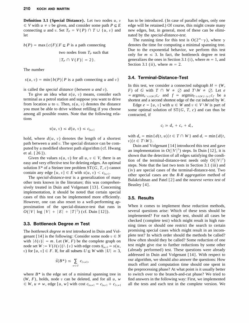
Tables VIII–X give computational results on real-world VLSI instances. One of the challenging problemsin the design of electronic circuits is the routing problem,which is, roughly speaking, the task to connect terminalsets via wires on a predefined area. Depending on theunderlying technology and the design rules, subproblemsarise that can be formulated as the problem of packingSteiner trees in certain graphs (see Lengauer [30] for anexcellent treatment of this subject) . The problems that weare going to consider result from seven different circuitsdescribed in Junger et al. [27]. The underlying graphsare grid graphs that contain holes. The holes result fromso-called cells that block certain areas of the grid. Thesets of terminals are located on the border of these holes.For each of the seven circuits and for each terminal setTi (where index i runs from 1 to the number of terminalsets of the circuit) , we constructed an instance of theSteiner tree problem. For the graph G , we have chosen theunderlying grid graph restricted to the minimal enclosingrectangle of the terminal set. The distance of two neigh-bored grid points in horizontal and vertical directions dif-fer for these circuits. This results in different edge costsfor horizontal and vertical edges in G .

In the library SteinLib, we put all instances with termi-nal sets whose cardinality is at least 10 (in total 475).The examples are distinguished by the name of the circuitfollowed by the index of the terminal set. For example,msm1234 means that the instance is defined by terminalset 1234 of circuit msm . As test problems for our algo-rithm, we chose for each circuit all instances whose twoleading nonzeros of the index of the terminal set differfrom the two leading nonzeros of all other indices. Ifthere are more than one index with the same two leadingnonzeros, we chose the instance with the smallest index(for instance, among examples msm3727, msm3731,msm3761 , and msm3786 , we chose msm3727) . In addi-tion, we added an instance with the smallest and largestnumber of terminals for each circuit. This way we ob-tained 116 different VLSI test instances.

The success of our branch-and-cut algorithm is shownin Tables VIII–X. We solve 83 out of the 116 instances tooptimality within 10,000 seconds and provide a solutionguarantee [(upper bound 0 lower bound)/ lower bound]of less than 10% for 85% of the examples. The biggestwith respect to number of terminals that we solve withinthe time limit are alue5067 and alue6735 with 68 termi-nals each. The biggest in size of the number of edges ismsm3727 with over 8000 edges. However, there are alsosmaller instances, for example, diw0795 with 10 termi-nals or msm2601 with less than 5000 variables after pre-solve, that we do not solve within the time limit. Allruns were performed with the default strategy (except fordiw0234 and alut2625) ; in particular, we applied Algo-rithm 3.2 to reduce the problem and did not perform a

TA

BLE

IV.

Co

ntin

ued

Ori

gina

lP

reso

lved

B&

CR

oot

LP

Tim

eS

olut

ions

Nam

eÉVÉ

ÉEÉ

ÉTÉ

ÉVÉ

ÉEÉ

ÉTÉ

Nod

Iter

Cut

sF

rac

Row

sN

ZP

reH

euL

PS

epT

otH

eu(1

)L

BU

B

p621

100

180

586

160

51

3518

80

151

1014

0.0

0.0

0.3

0.2

0.7

8741

8688

.086

88p6

2210

018

010

8715

910

125

224

019

313

140.

00.

00.

30.

20.

716

,546

15,9

72.0

15,9

72p6

2310

018

010

8615

610

127

277

023

415

230.

00.

00.

50.

20.

919

,496

19,4

96.0

19,4

96p6

2410

018

020

8114

214

116

187

017

297

00.

00.

00.

10.

10.

420

,246

20,2

46.0

20,2

46p6

2510

018

020

8415

120

121

317

028

218

910.

00.

10.

50.

31.

023

,677

23,0

78.0

23,0

78p6

2610

018

020

8114

320

117

252

022

413

890.

00.

10.

20.

20.

522

,346

22,3

46.0

22,3

46p6

2710

018

050

4773

241

1213

60

102

447

0.0

0.0

0.1

0.1

0.3

40,6

4740

,647

.040

.647

p628

100

180

5057

9429

115

180

016

086

90.

00.

00.

10.

10.

440

,008

40,0

08.0

40,0

08p6

2910

018

050

5385

251

1314

129

137

647

0.0

0.0

0.1

0.1

0.3

43,2

8743

,286

.543

,287

p630

200

370

1018

935

510

140

498

032

925

810.

00.

12.

40.

93.

626

,125

26,1

25.0

26,1

25p6

3120

037

020

185

342

201

3656

50

464

3253

0.0

0.2

1.7

0.9

3.1

39,1

9339

,067

.039

,067

p632

200

370

4017

732

234

125

692

056

740

830.

00.

22.

31.

13.

956

,562

56,2

17.0

56,2

17p6

3320

037

010

099

160

511

1629

60

253

1355

0.0

0.4

0.3

0.3

1.2

86,5

7386

,268

.086

,268

complete reduction test (see Section 3). If there is no time


222 KOCH AND MARTIN

TA

BLE

V.

Tes

tse

to

fS

ouk

upan

dC

how

Ori

gina

lP

reso

lved

B&

CR

oot

LP

Tim

eS

olut

ions

Nam

eÉVÉ

ÉEÉ

ÉTÉ

ÉVÉ

ÉEÉ

ÉTÉ

Nod

Iter

Cut

sF

rac

Row

sN

ZP

reH

euL

PS

epT

otH

eu(1

)L

BU

B

r01

1522

511

175

17

200

1971

0.0

0.0

0.0

0.0

0.0

187

187.

018

7

r02

1217

64

53

12

60

618

0.0

0.0

0.0

0.0

0.0

164

164.

016

4

r03

2845

719

327

112

600

5024

00.

00.

00.

00.

00.

123

723

6.0

236

r04

6411

28

4990

81

2320

90

145

1012

0.0

0.0

0.3

0.1

0.6

258

254.

025

4

r07

3049

1219

2912

110

540

4818

50.

00.

00.

00.

00.

125

424

8.0

248

r08

2437

1216

2212

15

370

3510

60.

00.

00.

00.

00.

123

623

6.0

236

r09

1522

710

147

13

170

1757

0.0

0.0

0.0

0.0

0.0

164

164.

016

4

r10

3660

624

436

112

580

5629

60.

00.

00.

10.

00.

117

717

7.0

177

r11

3049

621

356

17

330

3314

60.

00.

00.

00.

00.

114

414

4.0

144

r12

2742

922

369

113

730

5527

30.

00.

00.

10.

00.

118

018

0.0

180

r13

4271

932

549

113

105

092

465

0.0

0.0

0.1

0.1

0.2

150

150.

015

0

r14

3660

1210

146

12

140

1442

0.0

0.0

0.0

0.0

0.0

260

260.

026

0

r15

100

180

1489

165

141

2027

324

234

1567

0.0

0.1

0.4

0.2

0.8

150

147.

314

8

r17

4882

1034

6010

117

106

010

154

60.

00.

00.

10.

10.

220

020

0.0

200

r18

182

337

6215

626

452

121

477

042

421

720.

00.

60.

50.

52.

140

640

4.0

404

r19

168

310

1416

230

314

130

491

152

331

2606

0.1

0.1

1.9

0.8

3.0

190

187.

318

8

r21

1522

511

165

14

200

2074

0.0

0.0

0.0

0.0

0.0

192

192.

019

2

r22

1624

47

103

14

80

827

0.0

0.0

0.0

0.0

0.0

6363

.063

r23

1624

47

103

13

70

723

0.0

0.0

0.0

0.0

0.1

6565

.065

r24

1624

48

124

15

120

1243

0.0

0.0

0.0

0.0

0.0

3030

.030

r27

1624

46

93

14

80

826

0.0

0.0

0.0

0.0

0.1

133

133.

013

3

r28

1217

49

144

15

130

1348

0.0

0.0

0.0

0.0

0.0

2424

.024

r29

912

36

83

14

100

1037

0.0

0.0

0.0

0.0

0.1

200

200.

020

0

r30

2845

1219

3012

112

690

5726

20.

00.

00.

00.

00.

111

011

0.0

110

r31

130

237

1411

621

614

125

415

111

323

2375

0.0

0.1

1.3

0.4

1.9

267

258.

425

9

r32

210

391

1919

236

419

141

1069

294

541

5303

0.0

0.3

15.3

1.8

17.5

315

312.

131

3

r33

132

241

1813

224

118

130

474

172

351

2414

0.0

0.1

2.0

0.6

2.9

268

267.

126

8

r34

272

511

1925

949

219

162

1914

069

984

840.

10.

664

.74.

269

.825

724

1.0

241

r35

240

449

1822

843

218

150

1127

289

524

5047

0.0

0.4

16.8

2.2

19.7

159

150.

915

1

r37

4984

834

618

115

100

095

532

0.0

0.0

0.1

0.0

0.2

9090

.090

r38

100

180

1475

140

121

1825

036

220

1388

0.0

0.0

0.3

0.1

0.6

166

165.

516

6

r39

100

180

1470

130

121

1821

40

189

1157

0.0

0.0

0.2

0.2

0.5

166

166.

016

6

r40

6411

210

5497

101

2221

839

166

1017

0.0

0.0

0.3

0.1

0.5

155

154.

215

5

r41

144

263

2013

524

920

124

474

103

372

2514

0.0

0.1

1.3

0.5

2.1

224

223.

222

4

r42

8114

415

6912

715

117

221

4218

812

550.

00.

00.

30.

10.

615

415

2.3

153

r43

195

362

1617

933

516

146

1078

048

246

220.

10.

212

.41.

514

.425

825

5.0

255

r44

196

364

1717

633

117

155

1164

274

467

4879

0.1

0.3

16.1

2.0

18.6

256

251.

925

2

r45

270

507

1925

648

519

170

1865

315

686

8216

0.1

0.6

58.0

4.3

63.4

223

219.

722

0



TA

BLE

VI.

Tes

tse

t80

and

160

of

C.

Dui

n

Ori

gina

lF

inal

size

B&

CR

oot

LP

Tim

eS

olut

ions

Nam

eÉVÉ

ÉEÉ

ÉTÉ

ÉVÉ

ÉEÉ

ÉTÉ

RN

ItF

rac

Row

sN

ZH

LP

Sep

Tot

Heu

(1)

LB

UB

80.0

0180

120

680

120

60

115

098

657

0.0

0.1

0.0

0.2

1787

1787

.017

87

80.0

1180

350

677

195

61

156

2619

732

150.

00.

30.

30.

814

8214

78.2

1479

80.0

2180

3160

680

448

61

188

060

226

,151

0.0

2.1

2.8

5.5

1175

1175

.011

75

80.0

3180

160

680

160

60

118

010

082

20.

00.

00.

10.

215

7015

70.0

1570

80.0

4180

632

679

302

61

110

20

364

9827

0.0

1.3

1.0

2.5

1279

1276

.012

76

80.1

0180

120

880

120

80

115

010

362

10.

00.

00.

10.

126

0826

08.0

2608

80.1

1180

350

880

350

80

363

039

998

110.

12.

30.

84.

020

5120

25.4

2051

80.1

2180

3160

880

589

81

185

088

139

,730

0.1

3.4

3.4

7.5

1561

1561

.015

61

80.1

3180

160

880

160

80

136

020

216

630.

00.

10.

20.

422

8422

84.0

2284

80.1

4180

632

875

216

82

110

70

242

4654

0.1

1.7

1.5

3.5

1847

1788

.017

88

80.2

0180

120

1680

120

160

122

017

813

880.

00.

10.

10.

348

6247

60.0

4760

80.2

1180

350

1680

350

160

133

049

813

,993

0.0

1.5

0.6

2.3

3758

3631

.036

31

80.2

2180

3160

1680

1015

162

110

70

1489

70,5

860.

28.

812

.122

.131

5831

58.0

3158

80.2

3180

160

1680

160

160

118

026

426

360.

00.

10.

20.

444

5643

54.0

4354

80.2

4180

632

1680

632

160

115

913

305

499

47,9

350.

992

9.0

58.8

1097

.135

5134

87.1

3538

80.3

0180

120

2080

120

200

19

015

410

580.

00.

00.

10.

255

3055

19.0

5519

80.3

1180

350

2080

350

200

138

101

434

13,9

520.

07.

01.

38.

647

0845

53.0

4554

80.3

2180

3160

2080

783

203

122

40

1037

37,2

450.

510

.517

.329

.839

3239

32.0

3932

80.3

3180

160

2080

160

200

523

030

136

010.

00.

80.

21.

753

2152

04.5

5226

80.3

4180

632

2080

632

200

130

9566

430

,800

0.0

1.6

1.3

3.1

4316

4235

.142

36

160.

001

160

240

791

113

71

138

012

472

60.

00.

20.

20.

624

9624

90.0

2490

160.

011

160

812

711

019

37

21

660

176

2552

0.0

0.5

0.8

1.6

1757

1677

.016

77

160.

021

160

12,7

207

160

1049

71

116

40

1534

126,

445

0.2

29.5

21.0

53.4

1352

1352

.013

52

160.

031

160

320

797

122

71

134

092

545

0.0

0.2

0.2

0.5

2170

2170

.021

70

160.

041

160

2544

716

018

107

11

195

079

750

,471

0.4

12.6

15.4

29.3

1542

1494

.014

94

160.

101

160

240

1210

513

512

11

320

156

955

0.0

0.2

0.4

0.8

3859

3859

.038

59

160.

111

160

812

1213

827

812

11

530

295

5996

0.0

0.9

1.2

2.5

3059

2869

.028

69

160.

121

160

12,7

2012

160

932

126

112

170

1394

80,6

333.

858

1.8

214.

680

8.0

2363

2363

.023

63

160.

131

160

320

1211

517

412

11

430

160

1417

0.0

0.4

0.5

1.3

3356

3356

.033

56

160.

141

160

2544

1213

555

612

41

254

067

427

,248

0.4

25.4

15.5

42.8

2549

2549

.025

49

160.

201

160

240

2416

024

024

05

240

352

3860

0.1

0.6

0.6

1.9

7117

6909

.069

23

160.

211

160

812

2416

081

224

015

470

344

786

45,2

081.

210

32.8

74.6

1143

.557

3555

40.3

5583

160.

221

160

12,7

2024

160

2380

245

179

811

846

9849

9,30

56.

254

7.5

325.

288

9.1

4729

4728

.647

29

160.

231

160

320

2416

032

024

01

240

497

6911

0.1

1.3

0.7

2.3

6810

6662

.066

62

160.

241

160

2544

2416

025

4424

012

118

0273

114

6933

2,82

98.

719

,156

.611

62.0

21,0

08.6

5186

5034

.750

86

160.

301

160

240

4016

024

040

01

110

425

3676

0.0

0.3

0.3

1.1

11,9

0911

,816

.011

,816

160.

311

160

812

4016

081

240

025

356

346

1055

46,6

981.

656

0.0

82.4

687.

995

1090

83.9

9135

160.

321

160

12,7

2040

160

12,7

2040

09

160

1125

3806

1,29

7,79

45.

116

13.9

1179

.929

59.4

7903

7871

.478

76

160.

331

160

320

4016

032

040

01

160

666

9274

0.1

0.4

0.8

1.8

10,8

2010

,414

.010

,414

160.

341

160

2544

4016

025

4440

013

128

3799

614

8534

6,17

123

.250

,712

.027

50.5

54,5

00.7

8558

8277

.983

31


224 KOCH AND MARTIN

TA

BLE

VII.

Tes

tse

t32

0an

d64

0o

fC

.D

uin

Ori

gina

lF

inal

size

B&

CR

oot

LP

Tim

eS

olut

ions

Nam

eÉVÉ

ÉEÉ

ÉTÉ

ÉVÉ

ÉEÉ

ÉTÉ

RN

ItF

rac

Row

sN

ZH

LP

Sep

Tot

Heu

(1)

LB

UB

320.

001

320

480

814

417

48

11

510

153

913

0.1

0.3

0.7

1.3

2672

2672

.026

72

320.

011

320

1845

888

177

84

327

20

254

4184

0.3

13.9

10.0

25.5

2057

2049

.520

53

320.

021

320

51,0

408

320

2227

83

145

30

3578

581,

443

4.4

409.

165

9.1

1102

.015

6415

53.0

1553

320.

031

320

640

832

064

08

03

920

582

9176

0.1

5.8

3.1

10.5

2709

2660

.026

73

320.

041

320

10,2

088

7817

58

81

895

025

946

104.

418

2.5

239.

243

4.6

1750

1707

.017

07

320.

101

320

480

1716

019

017

11

360

190

1037

0.0

0.3

0.9

1.7

5548

5548

.055

48

320.

111

320

1845

1732

018

4517

07

168

116

1175

41,1

410.

714

9.8

42.1

206.

544

3542

53.4

4273

320.

121

320

51,0

4017

320

2046

178

111

150

2619

218,

395

17.7

621.

619

09.0

2595

.333

2133

21.0

3321

320.

131

320

640

1732

064

017

01

450

770

11,3

000.

13.

63.

57.

453

5352

55.0

5255

320.

141

320

10,2

0817

320

10,2

0817

045

834

183

2993

632,

380

11.2

8188

.614

76.2

10,1

39.9

3701

3567

.936

06

320.

201

320

480

3432

048

034

01

330

708

7595

0.2

1.3

2.9

5.0

10,2

7510

,044

.010

,044

320.

211

320

1845

3432

018

4534

049

1254

517

1829

117,

293

9.9

7121

.492

2.4

8274

.684

7679

87.8

8039

320.

221

320

51,0

4034

320

15,7

2634

21

624

267

10,2

143,

936,

831

69.0

3846

.760

40.0

10,0

19.4

6697

6664

.066

79

320.

231

320

640

3432

064

034

07

5272

932

23,0

550.

322

.48.

339

.510

,028

9855

.898

62

320.

241

320

10,2

0834

320

10,2

0834

015

344

1003

4756

865,

964

8.3

8389

.413

87.4

10,0

07.7

7214

6985

.470

27

320.

301

320

480

8032

048

080

01

190

1067

19,0

370.

32.

13.

913

.323

,669

23,2

79.0

23,2

79

320.

311

320

1845

8032

018

4580

097

1101

503

1778

83,5

6826

.777

54.0

1788

.610

,006

.618

,843

17,7

44.9

17,9

45

320.

321

320

51,0

4080

320

51,0

4080

01

8411

8279

944,

372,

292

39.5

5323

.649

72.2

10,3

68.9

15,8

6315

,609

.615

,771

320.

331

320

640

8032

064

080

033

124

012

0624

,025

2.0

159.

145

.926

6.7

22,3

5121

,460

.721

,517

320.

341

320

10,2

0880

320

10,2

0880

03

106

1563

6219

1,62

0,17

57.

387

85.2

1096

.910

,021

.516

,463

16,1

50.3

16,3

74

640.

001

640

960

933

549

11

510

101

571

0.0

0.5

1.0

5.2

4183

4033

.040

33

640.

011

640

4135

945

919

31

121

011

987

30.

22.

36.

318

.823

9223

92.0

2392

640.

021

640

204,

480

964

052

159

31

818

082

342,

633,

466

23.5

4358

.563

69.4

11,0

04.9

1749

1749

.017

49

640.

031

640

1280

920

925

49

21

960

207

1330

0.2

1.8

3.0

6.5

3278

3278

.032

78

640.

041

640

40,8

969

111

340

97

180

648

437

10,5

6521

.142

2.2

1732

.322

14.9

1945

1896

.318

97

640.

101

640

960

2538

451

525

11

670

640

8418

0.4

15.0

8.2

26.7

9054

8764

.087

64

640.

111

640

4135

2564

041

3525

083

1935

371

3204

133,

572

24.0

11,5

37.8

1655

.613

,677

.564

1560

79.4

6167

640.

121

640

204,

480

2564

020

4,48

025

01

5936

2360

2,12

2,20

845

.820

9.5

9710

.810

,158

.649

0647

41.2

4906

640.

131

640

1280

2538

751

725

11

760

576

7774

0.4

13.6

11.5

28.6

8319

8097

.080

97

640.

141

640

40,8

9625

640

40,8

9625

03

230

209

6401

1,53

6,07

629

.763

78.3

3432

.310

,059

.253

0751

41.9

5247

640.

201

640

960

5064

096

050

03

390

1516

25,6

100.

711

.710

.131

.316

,797

16,0

78.0

16,0

79

640.

211

640

4135

5064

041

3550

01

245

1149

3746

297,

821

7.3

9297

.269

0.2

10,0

02.7

12,7

1411

,793

.812

,291

640.

221

640

204,

480

5064

020

4,48

050

01

5054

3517

2,94

7,25

188

.027

2.5

9656

.310

,219

.698

7695

42.4

9876

640.

231

640

1280

5064

012

8050

023

185

416

1707

43,7

702.

762

7.7

103.

680

4.1

15,2

0114

,974

.815

,014

640.

241

640

40,8

9650

640

40,8

9650

01

139

1008

10,4

882,

692,

998

33.4

7544

.225

00.2

10,1

02.6

10,3

8610

,136

.010

,338

640.

301

640

960

160

640

960

160

01

220

2061

54,0

984.

715

.720

.315

2.3

46,1

0445

,005

.045

,005

640.

311

640

4135

160

640

4135

160

03

184

1741

4644

193,

418

40.5

8394

.514

17.8

10,0

39.2

37,7

0635

,256

.936

,562

640.

321

640

204,

480

160

640

204,

480

160

01

300

6108

4,77

7,10

017

0.1

388.

191

74.5

10,0

58.1

31,7

5730

,594

.031

,757

640.

331

640

1280

160

640

1280

160

055

507

678

2209

118,

490

79.2

2227

.310

77.9

3817

.944

,711

42,7

54.7

42,7

96

640.

341

640

40,8

9616

064

040

,896

160

01

6323

5417

,086

7,17

6,82

159

.074

69.7

2697

.410

,332

.232

,303

31,8

40.6

32,3

03



TA

BLE

VIII

.V

LSI

exam

ple

s:d

iwan

dta

q

Ori

gina

lP

reso

lved

B&

CR

oot

LP

Tim

eS

olut

ions

Nam

eÉVÉ

ÉEÉ

ÉTÉ

ÉVÉ

ÉEÉ

ÉTÉ

Nod

Iter

Cut

sF

rac

Row

sN

ZP

reH

euL

PS

epT

otH

eu(1

)L

BU

B

diw

0234

a53

4910

,086

2538

5672

6624

139

610

,928

725

5113

54,4

9212

,657

.366

.910

,554

.271

7.3

24,0

02.9

2001

1995

.119

96

diw

0250

353

608

1130

854

511

157

584

050

533

870.

10.

32.

71.

85.

135

035

0.0

350

diw

0260

539

985

1251

895

411

167

628

060

638

910.

10.

72.

11.

85.

146

846

8.0

468

diw

0313

468

822

1442

175

212

150

619

7150

034

300.

10.

42.

92.

56.

139

739

6.7

397

diw

0393

212

381

1119

435

311

140

460

038

527

820.

00.

11.

60.

93.

030

230

2.0

302

diw

0445

1804

3311

3317

4532

4033

123

965

9110

6029

2629

,613

0.7

23.7

2664

.813

6.7

2827

.613

8713

62.3

1363

diw

0459

3636

6789

2535

1666

3525

159

011

,569

1318

5022

49,9

902.

710

2.0

8014

.350

6.1

8628

.613

6713

61.1

1362

diw

0460

339

579

1329

652

313

129

433

039

624

400.

10.

10.

80.

92.

235

834

5.0

345

diw

0473

2213

4135

2521

4040

4625

136

258

8270

136

0135

,557

1.1

34.4

1658

.317

2.9

1868

.611

0710

97.1

1098

diw

0487

2414

4386

2522

9442

3325

146

752

950

3117

24,0

081.

246

.356

8.8

166.

178

4.7

1451

1424

.014

24

diw

0495

938

1655

1089

416

0310

119

415

3410

911

6280

670.

23.

322

.713

.740

.762

661

5.5

616

diw

0513

918

1684

1086

716

2110

115

721

4746

714

5912

,461

0.2

2.7

106.

119

.812

9.4

614

603.

360

4

diw

0523

1080

2015

1010

2519

4310

126

721

3463

1663

14,3

830.

35.

315

6.5

24.9

188.

156

156

0.7

561

diw

0540

286

465

1023

239

410

137

389

033

419

530.

00.

10.

91.

02.

237

437

4.0

374

diw

0559

3738

7013

1836

2768

8318

127

211

,148

1501

4484

50,5

572.

837

.695

89.4

437.

610

,070

.015

7813

73.9

1570

diw

0778

7231

13,7

2724

7145

13,6

2924

120

012

,428

1867

6585

69,6

3210

.179

.590

15.5

1026

.910

,135

.721

9718

00.3

2173

diw

0779

11,8

2122

,516

5011

,715

22,3

9950

114

115

,341

2594

9499

82,3

6628

.325

5.0

7111

.227

67.7

10,1

67.2

4588

3158

.345

66

diw

0795

3221

5938

1031

0157

9210

129

899

9317

6247

2057

,537

2.1

21.9

9715

.533

3.0

10,0

74.8

1584

1455

.715

53

diw

0801

3023

5575

1028

8154

0010

126

999

1918

1545

9757

,572

1.9

18.2

9689

.632

4.8

10,0

36.6

1598

1528

.315

87

diw

0819

10,5

5320

,066

3210

,447

19,9

4232

114

012

,691

2318

7923

76,6

4122

.513

3.0

8681

.914

26.5

10,2

67.9

3467

2458

.834

30

diw

0820

11,7

4922

,384

3711

,634

22,2

5337

115

615

,756

2502

10,1

7193

,809

28.0

202.

981

69.4

1734

.310

,139

.042

7128

66.8

4259

taq0

014

6466

11,0

4612

860

2910

,563

128

168

14,1

9636

2082

9269

,417

7.6

230.

295

78.2

714.

410

,536

.255

1346

88.3

5442

taq0

023

572

963

1150

187

311

194

1691

088

479

460.

10.

960

.27.

569

.262

362

1.0

621

taq0

365

4186

7074

2238

3066

8122

135

010

,958

2036

4917

54,0

793.

456

.192

96.8

663.

610

,023

.319

7118

19.2

1914

taq0

377

6836

11,7

1513

664

3311

,301

136

156

13,9

3641

4490

9574

,502

8.7

256.

194

61.3

689.

210

,421

.366

5956

40.5

6565

taq0

431

1128

1905

1399

517

4513

113

936

3773

815

6415

,975

0.3

3.0

516.

137

.955

8.1

937

896.

189

7

taq0

631

609

932

1047

578

210

160

1114

311

624

4752

0.1

0.4

23.1

6.0

29.9

594

580.

558

1

taq0

739

837

1438

1677

313

6216

391

2890

5513

1813

,277

0.2

30.9

308.

420

.636

0.8

859

847.

184

8

taq0

741

712

1217

1663

611

1516

110

931

8673

312

1013

,877

0.1

1.7

385.

618

.540

6.6

865

846.

484

7

taq0

751

1051

1791

1694

516

6316

198

3467

793

1672

16,5

330.

22.

348

6.1

27.4

516.

895

293

8.2

939

taq0

891

331

560

1026

947

610

182

624

180

473

3457

0.1

0.4

4.5

2.2

7.5

319

318.

531

9

taq0

903

6163

10,4

9013

056

5299

0713

01

6213

,612

3593

7552

66,1

386.

921

2.0

9655

.860

4.7

10,4

84.6

5208

4510

.351

62

taq0

910

310

514

1725

443

715

129

429

037

625

660.

00.

11.

01.

02.

437

037

0.0

370

taq0

920

122

194

1764

105

131

1299

092

451

0.0

0.0

0.0

0.1

0.2

210

210.

021

0

taq0

978

777

1239

1067

011

2410

175

938

068

447

090.

11.

09.

38.

619

.456

656

6.0

566

aT

his

run

was

perf

orm

edw

ith

the

defa

ult

para

met

erse

ttin

gex

cept

that

the

com

plet

ere

duct

ion

test

was

used

and

noti

me

lim

itw

asgi

ven.


226 KOCH AND MARTIN

TA

BLE

IX.

VLS

Iex

amp

les:

dm

xan

dm

sm

Ori

gina

lP

reso

lved

B&

CR

oot

LP

Tim

eS

olut

ions

Nam

eÉVÉ

ÉEÉ

ÉTÉ

ÉVÉ

ÉEÉ

ÉTÉ

Nod

Iter

Cut

sF

rac

Row

sN

ZP

reH

euL

PS

epT

otH

eu(1

)L

BU

B

dmxa

0296

233

386

1219

233

212

140

425

5534

922

170.

00.

11.

30.

82.

534

934

3.5

344

dmxa

0368

2050

3676

1819

4235

5818

127

449

5510

1627

8524

,254

0.9

16.7

1120

.513

4.3

1274

.010

2110

16.1

1017

dmxa

0454

1848

3286

1617

4731

6516

119

541

6878

025

7322

,149

0.7

9.5

500.

478

.259

0.1

964

913.

691

4

dmxa

0628

169

280

1014

424

910

137

400

132

319

2279

0.0

0.1

1.7

0.6

2.6

277

274.

327

5

dmxa

0734

663

1154

1162

111

0311

111

115

3432

897

280

730.

11.

480

.811

.093

.851

950

5.4

506

dmxa

0848

499

861

1644

378

916

153

1341

087

272

210.

10.

529

.15.

635

.760

059

4.0

594

dmxa

0903

632

1087

1055

898

910

195

1917

411

975

9000

0.1

1.0

94.0

9.2

104.

859

857

9.2

580

dmxa

1010

3983

7108

2337

3168

1723

181

210

,320

870

4390

42,2

583.

111

8.9

9107

.078

5.5

10,0

19.1

1497

1407

.214

88

dmxa

1109

343

559

1729

650

217

137

728

049

335

090.

10.

34.

62.

07.

145

445

4.0

454

dmxa

1200

770

1383

2172

113

2221

169

2043

306

1331

11,8

290.

21.

511

7.4

11.6

131.

476

274

9.6

750

dmxa

1304

298

503

1026

546

110

139

507

044

129

120.

00.

21.

81.

53.

831

231

1.0

311

dmxa

1516

720

1269

1166

712

0411

112

313

7629

189

466

700.

11.

828

.511

.242

.251

150

7.5

508

dmxa

1721

1005

1731

1892

316

4018

117

916

9913

813

5110

,025

0.3

4.8

28.9

15.6

50.3

784

779.

778

0

dmxa

1801

2333

4137

1721

1838

9017

119

188

6915

4831

2542

,989

1.1

12.3

7063

.018

0.5

7259

.214

2313

64.2

1365

msm

0580

338

541

1127

345

911

147

708

051

736

360.

00.

25.

61.

67.

848

046

7.0

467

msm

0654

1290

2270

1011

6321

1310

123

729

3159

118

1015

,492

0.4

5.3

210.

945

.726

3.2

823

822.

682

3

msm

0709

1442

2403

1612

8022

1116

197

2973

016

0813

,760

0.5

3.3

206.

235

.624

6.4

884

884.

088

4

msm

0920

752

1264

2664

311

2726

153

1739

011

3485

350.

11.

534

.110

.046

.382

180

6.0

806

msm

1008

402

695

1136

764

911

159

1093

304

655

5565

0.1

0.4

19.9

3.3

23.9

504

493.

449

4

msm

1234

933

1632

1386

515

4811

117

618

5739

410

8187

880.

23.

090

.526

.512

0.9

550

549.

355

0

msm

1477

1199

2078

3110

7419

1531

186

2768

5216

3114

,427

0.3

5.0

234.

920

.926

2.0

1096

1067

.510

68

msm

1707

278

478

1123

842

011

147

339

032

318

950.

00.

20.

80.

81.

956

456

4.0

564

msm

1844

9013

510

6095

101

1514

30

133

623

0.0

0.0

0.1

0.1

0.2

191

188.

018

8

msm

1931

875

1522

1079

514

218

118

817

2036

711

3587

070.

22.

556

.815

.775

.760

460

3.8

604

msm

2000

898

1562

1081

414

569

121

020

2444

411

8299

800.

22.

990

.319

.011

3.2

594

593.

559

4

msm

2152

2132

3702

3719

9635

3637

110

566

9714

3828

7131

,772

1.0

14.1

2861

.613

3.5

3011

.716

3415

89.1

1590

Tab

leIX

cont

inue

s



TA

BLE

IX.

Co

ntin

ued

Ori

gina

lP

reso

lved

B&

CR

oot

LP

Tim

eS

olut

ions

Nam

eÉVÉ

ÉEÉ

ÉTÉ

ÉVÉ

ÉEÉ

ÉTÉ

Nod

Iter

Cut

sF

rac

Row

sN

ZP

reH

euL

PS

epT

otH

eu(1

)L

BU

B

msm

2326

418

723

1438

368

214

135

677

052

938

440.

10.

33.

52.

66.

740

439

9.0

399

msm

2492

4045

7094

1238

1268

1512

168

111

,530

1173

4836

45,3

213.

263

.991

76.8

754.

710

,002

.014

6014

28.7

1459

msm

2525

3031

5239

1227

8049

5312

140

462

8511

9037

5932

,556

2.0

28.3

1618

.523

5.6

1886

.513

0312

89.1

1290

msm

2601

2961

5100

1627

1148

2916

128

498

3815

9037

1241

,758

1.8

21.1

9704

.331

1.3

10,0

43.5

1474

1403

.614

40

msm

2705

1359

2458

1312

9523

8113

111

429

540

1682

15,4

800.

43.

532

8.8

37.3

370.

873

071

4.0

714

msm

2802

1709

2963

1815

6728

0418

117

136

620

2043

17,0

260.

68.

734

7.3

70.7

428.

493

692

6.0

926

msm

2846

3263

5783

8931

4056

3789

111

112

,358

2597

4935

55,7

242.

291

.996

68.4

501.

010

,268

.432

0831

03.7

3141

msm

3277

1704

2991

1215

6428

3212

126

737

8135

021

9819

,426

0.6

9.4

532.

071

.761

4.9

869

868.

486

9

msm

3676

957

1554

1080

313

6710

112

518

4232

210

3980

300.

21.

776

.615

.995

.161

260

6.8

607

msm

3727

4640

8255

2143

9179

8821

145

810

,565

048

0743

,464

4.1

93.8

6646

.791

7.7

7665

.914

0613

76.0

1376

msm

3829

4221

7255

1238

9568

8112

153

311

,617

1444

4747

44,0

593.

560

.393

74.0

629.

210

,070

.416

1213

84.6

1571

msm

4038

237

390

1118

131

311

159

515

112

366

2562

0.0

0.2

2.3

1.3

3.9

353

352.

435

3

msm

4114

402

690

1635

262

516

143

684

2951

036

140.

10.

33.

62.

76.

939

339

2.2

393

msm

4190

391

666

1634

060

216

139

763

209

586

4451

0.1

0.3

6.0

2.1

8.7

381

380.

738

1

msm

4224

191

302

1115

625

811

138

417

134

313

2018

0.0

0.1

1.8

0.6

2.6

315

310.

831

1

msm

4312

5181

8893

1048

0084

6410

137

110

,370

1947

5678

58,7

385.

045

.492

86.3

679.

110

,019

.420

5516

84.2

2049

msm

4414

317

476

1122

536

511

132

426

129

326

1909

0.0

0.1

1.3

0.7

2.2

408

407.

640

8

msm

4515

777

1358

1373

413

0613

193

2175

453

1238

11,2

000.

21.

414

8.4

15.8

166.

464

062

9.4

630


228 KOCH AND MARTIN

TA

BLE

X.

VLS

Iex

amp

les:

gap

,al

ue,

and

alu

t

Ori

gina

lP

reso

lved

B&

CR

oot

LP

Tim

eS

olut

ions

Nam

eÉVÉ

ÉEÉ

ÉTÉ

ÉVÉ

ÉEÉ

ÉTÉ

Nod

Iter

Cut

sF

rac

Row

sN

ZP

reH

euL

PS

epT

otH

eu(1

)L

BU

B

gap1

307

342

552

1728

348

517

134

626

118

517

3401

0.0

0.2

2.5

1.7

4.8

554

548.

154

9

gap1

413

541

906

1046

581

510

162

932

067

450

060.

10.

411

.34.

416

.645

745

7.0

457

gap1

500

220

374

1716

629

312

169

284

4723

515

460.

00.

20.

70.

71.

925

425

3.2

254

gap1

810

429

702

1735

460

417

138

600

047

630

030.

10.

32.

22.

14.

949

048

2.0

482

gap1

904

735

1256

2167

311

8321

151

1385

131

1088

7755

0.1

1.2

15.4

8.1

25.4

778

762.

676

3

gap2

007

2039

3548

1718

9433

6917

725

866

4560

2487

24,8

500.

919

5.4

2048

.216

3.6

2410

.011

2011

03.4

1104

gap2

119

1724

2975

2915

5727

7229

185

4427

023

7922

,744

0.6

6.7

748.

360

.381

7.1

1269

1244

.012

44

gap2

740

1196

2084

1410

8019

3414

114

935

4749

616

2416

,078

0.3

4.2

578.

939

.062

3.1

745

744.

374

5

gap2

800

386

653

1232

857

712

165

824

060

344

630.

10.

49.

62.

913

.238

738

6.0

386

gap2

975

179

293

1015

626

710

140

316

027

716

820.

00.

10.

80.

51.

624

524

5.0

245

gap3

036

346

583

1330

853

513

143

912

288

567

4782

0.1

0.3

12.3

2.1

15.1

469

456.

345

7

gap3

100

921

1558

1179

213

9311

115

823

6357

913

0112

,083

0.2

2.3

156.

319

.317

8.9

642

639.

264

0

gap3

128

10,3

9318

,043

104

9711

17,3

0810

41

120

11,6

8925

0359

0054

,435

20.3

377.

668

25.8

2790

.210

,021

.143

8636

16.3

4315

alue

2087

1244

1971

3496

216

5034

147

2047

013

7110

,383

0.3

2.8

63.0

15.6

82.4

1065

1049

.010

49

alue

2105

1220

1858

3491

115

1034

111

818

140

1290

10,0

910.

35.

738

.423

.568

.710

3910

32.0

1032

alue

3146

3626

5869

6430

4752

2364

123

188

5411

3140

2238

,092

2.3

87.7

9403

.758

7.3

10,0

85.0

2280

2215

.022

40

alue

5067

3524

5560

6828

5048

1968

110

179

770

3553

34,7

892.

145

.434

14.2

345.

938

09.9

2622

2586

.025

86

alue

5345

5179

8165

6842

7072

0268

112

610

,940

2533

5199

49,7

674.

489

.097

21.4

446.

110

,264

.636

0333

18.6

3560

alue

5623

4472

6938

6835

8960

0068

110

310

,241

2405

4611

46,0

443.

463

.298

11.4

335.

210

,216

.035

0932

58.1

3463

alue

5901

11,5

4318

,429

6897

4416

,553

681

9711

,544

1836

6443

56,9

5022

.419

4.9

8376

.214

83.4

10,0

81.3

4042

3418

.639

94

alue

6179

3372

5213

6727

0145

0266

512

076

2061

3380

29,7

461.

928

8.7

3989

.428

9.8

4573

.124

8324

52.0

2452

alue

6457

3932

6137

6832

3354

0368

110

710

,701

2161

4458

45,2

142.

558

.296

43.1

390.

610

,097

.331

1330

05.3

3062

alue

6735

4119

6696

6835

0160

2168

173

7693

040

2837

,632

3.0

42.4

3839

.525

5.7

4142

.927

3526

96.0

2696

alue

6951

2818

4419

6722

7438

4367

195

5810

027

8026

,221

1.4

31.3

1375

.619

0.2

1600

.424

8323

86.0

2386

alue

7065

34,0

4654

,841

544

29,2

4349

,948

544

122

12,4

5613

6111

,351

59,3

4210

26.3

6328

.522

8.9

2422

.410

,042

.924

,827

12,5

89.4

24,8

27

alue

7066

6405

10,4

5416

5516

9506

151

390

10,9

0717

4956

2152

,684

6.9

74.2

8994

.697

1.4

10,0

50.3

2285

1767

.922

75

alue

7080

a34

,479

55,4

9423

44—

——

——

——

——

——

——

——

——

alue

7229

940

1474

3473

012

3434

110

413

550

1115

8254

0.2

3.7

17.4

10.5

32.7

824

824.

082

4

alut

0787

1160

2089

3411

0520

2334

110

725

480

1759

14,3

320.

36.

514

8.9

27.7

184.

498

798

2.0

982

alut

0805

966

1666

3485

215

3634

158

2634

512

1372

12,1

860.

22.

718

4.9

18.2

206.

997

995

7.4

958

alut

1181

3041

5693

6429

4955

7164

199

10,5

4021

6547

2253

,720

1.9

43.9

9914

.024

7.9

10,2

10.4

2462

2261

.023

90

alut

2010

6104

11,0

1168

5777

10,6

3468

113

412

,720

2717

6805

64,3

827.

015

4.9

9208

.069

5.5

10,0

69.7

3403

3218

.033

22

alut

2288

9070

16,5

9568

8824

16,3

2968

198

13,0

9728

9879

5873

,484

15.7

186.

289

80.5

1013

.410

,200

.339

5332

91.7

3889

alut

2566

5021

9055

6847

5987

4667

110

411

,235

2508

5543

54,0

874.

783

.595

69.6

689.

510

,350

.631

2929

00.7

3127

alut

2610

33,9

0162

,816

204

33,2

0762

,084

204

159

17,2

6931

1514

,250

106,

987

1153

.022

60.8

2722

.143

16.0

10,4

70.0

12,7

9769

25.9

12,7

60

alut

2625

b36

,711

68,1

1787

936

,137

67,5

2687

91

5077

,716

770

19,9

9111

4,26

940

9.4

3347

.729

1.8

6177

.710

,299

.336

,763

19,5

45.0

36,7

63

alut

2764

387

626

3432

053

932

178

590

1554

028

590.

11.

31.

92.

86.

565

763

9.5

640

aW

eha

veno

tbe

enab

leto

solv

eth

isin

stan

ceon

any

ofou

rw

orks

tati

ons;

the

mem

ory

requ

irem

ents

are

mor

eth

an1

Gig

abyt

e.b

Thi

sru

nw

aspe

rfor

med

ona

Sun

Ult

ra1

Mod

el17

0Ew

ith

the

foll

owin

gpa

ram

eter

chan

ges:

The

prim

alhe

uris

tic

was

call

edev

ery

50it

erat

ions

(def

ault

is5)

and

the

term

inal

-dis

tanc

e-te

st(S

tep

(4)

ofA

lgor

ithm

3.2)

was

skip

ped.



TA

BLE

XI.

Rec

tilin

ear

test

sets

es10

and

es20

Ori

gina

lP

reso

lved

B&

CR

oot

LP

Tim

eS

olut

ions

Nam

eÉVÉ

ÉEÉ

ÉTÉ

ÉVÉ

ÉEÉ

ÉTÉ

Nod

Iter

Cut

sF

rac

Row

sN

ZP

reH

euL

PS

epT

otH

eu(1

)L

BU

B

es10

a57

9410

5390

101

3124

30

182

1090

0.0

0.1

0.5

0.2

0.8

23,0

90,7

4722

,920

,745

.022

,920

,745

es10

b56

9210

5083

101

2721

80

155

883

0.0

0.0

0.3

0.1

0.6

19,1

34,1

0419

,134

,104

.019

,134

,104

es10

c58

9610

5492

101

2117

10

146

778

0.0

0.0

0.2

0.1

0.4

26,1

26,9

8026

,003

,678

.026

,003

,678

es10

d50

8010

4676

101

2214

80

128

689

0.0

0.0

0.2

0.1

0.3

20,4

61,1

1620

,461

,116

.020

,461

,116

es10

e63

106

1059

102

101

1614

80

138

738

0.0

0.0

0.1

0.1

0.3

18,8

18,9

1618

,818

,916

.018

,818

,916

es10

f51

8210

4677

91

2820

90

157

909

0.0

0.0

0.3

0.2

0.5

26,8

31,3

8126

,540

,768

.026

,540

,768

es10

g48

7610

3863

81

1412

30

109

547

0.0

0.0

0.1

0.1

0.2

26,0

25,0

7226

,025

,072

.026

,025

,072

es10

h55

9010

5186

101

2119

90

160

882

0.0

0.0

0.2

0.1

0.5

25,0

56,2

1425

,056

,214

.025

,056

,214

es10

i53

8610

4779

91

1816

00

135

747

0.0

0.0

0.1

0.1

0.4

22,0

62,3

5522

,062

,355

.022

,062

,355

es10

j50

8010

4575

91

1313

30

124

617

0.0

0.0

0.1

0.0

0.3

24,1

03,2

4823

,936

,095

.023

,936

,095

es10

k51

8210

4778

101

2614

50

121

632

0.0

0.0

0.3

0.1

0.5

22,2

39,5

3522

,239

,535

.022

,239

,535

es10

l53

8610

4881

91

1611

90

110

531

0.0

0.0

0.0

0.1

0.3

19,6

26,3

1819

,626

,318

.019

,626

,318

es10

m45

7010

4065

91

1512

00

111

531

0.0

0.0

0.1

0.1

0.3

19,4

83,9

1419

,483

,914

.019

,483

,914

es10

n37

5410

2946

71

1692

076

335

0.0

0.0

0.1

0.0

0.2

21,8

56,1

2821

,856

,128

.021

,856

,128

es10

o45

7010

3761

71

2197

2085

417

0.0

0.0

0.1

0.0

0.2

18,6

41,9

2418

,641

,924

.018

,641

,924

es20

a27

350

620

269

502

201

7316

560

737

6926

0.1

0.6

27.9

4.3

33.4

33,7

33,7

8733

,703

,886

.033

,703

,886

es20

b28

152

220

277

518

201

5415

510

716

6764

0.1

0.5

28.3

3.5

32.8

33,2

25,8

5332

,639

,486

.032

,639

,486

es20

c22

541

020

221

406

201

4711

060

584

4666

0.2

0.4

8.7

2.1

11.6

28,5

28,7

5727

,847

,417

.027

,847

,417

es20

d26

949

820

265

494

205

110

2448

7266

869

370.

123

.274

.97.

210

6.3

27,6

86,6

8127

,624

,394

.027

,624

,394

es20

e27

150

220

267

498

203

6917

0846

724

6858

0.1

10.2

43.4

4.7

59.1

34,5

31,0

7634

,033

,163

.034

,033

,163

es20

f27

250

420

267

499

191

7113

050

671

5976

0.1

0.6

15.4

3.6

20.1

36,4

12,5

9636

,014

,241

.036

,014

,241

es20

g27

350

620

269

502

201

7018

010

694

7314

0.1

0.6

42.6

4.8

48.5

35,4

18,8

5634

,934

,874

.034

,934

,874

es20

h24

044

020

235

435

193

7318

4524

609

6542

0.1

10.4

38.5

4.1

53.9

38,7

19,1

2938

,016

,346

.038

,016

,346

es20

i28

653

220

282

528

201

4814

420

695

6433

0.1

0.5

23.6

3.4

27.9

36,7

39,9

3936

,739

,939

.036

,739

,939

es20

j25

246

420

248

460

201

5113

380

647

5951

0.1

0.4

18.4

2.7

21.9

34,8

72,0

8834

,024

,740

.034

,024

,740

es20

k27

050

020

266

496

201

8017

620

647

6615

0.2

0.7

35.4

5.2

41.9

27,3

37,0

9927

,123

,908

.027

,123

,908

es20

l25

547

020

251

466

201

5916

660

652

6614

0.1

0.5

36.7

3.5

41.1

30,9

11,1

5930

,451

,397

.030

,451

,397

es20

m24

645

220

241

447

191

5811

420

663

5742

0.1

0.4

13.2

2.6

16.7

34,5

52,1

8334

,438

,673

.034

,438

,673

es20

n25

246

420

248

460

201

6717

690

671

7122

0.1

0.6

34.2

4.2

39.6

34,0

62,3

7434

,062

,374

.034

,062

,374

es20

o24

745

420

242

449

191

4312

560

620

5399

0.1

0.3

16.8

2.6

20.0

32,5

82,3

0932

,303

,746

.032

,303

,746


230 KOCH AND MARTIN

TA

BLE

XII.

Rec

tilin

ear

test

sets

es30

and

es40

Ori

gina

lP

reso

lved

B&

CR

oot

LP

Tim

eS

olut

ions

Nam

eÉVÉ

ÉEÉ

ÉTÉ

ÉVÉ

ÉEÉ

ÉTÉ

Nod

Iter

Cut

sF

rac

Row

sN

ZP

reH

euL

PS

epT

otH

eu(1

)L

BU

B

es30

a66

412

6830

660

1264

301

120

6045

014

8320

,589

0.2

4.4

790.

137

.983

3.7

41,4

45,9

9440

,692

,993

.040

,692

,993

es30

b64

612

3230

642

1228

303

171

7156

5114

8521

,423

0.2

35.6

1223

.554

.813

15.6

41,7

99,7

7540

,900

,061

.040

,900

,061

es30

c65

912

5830

655

1254

301

289

12,6

900

1461

21,7

620.

210

.138

77.9

115.

440

05.2

44,1

36,2

2843

,120

,444

.043

,120

,444

es30

d67

712

9430

673

1290

301

161

7134

014

4018

,779

0.2

5.8

1506

.057

.015

70.1

42,9

61,4

6842

,150

,958

.042

,150

,958

es30

e66

012

6030

656

1256

301

177

7380

014

6920

,352

0.2

6.4

1473

.556

.315

37.5

41,9

51,2

2641

,739

,748

.041

,739

,748

es30

f60

611

5230

602

1148

301

188

7456

014

1521

,015

0.2

6.2

1203

.459

.312

70.3

40,8

08,5

1739

,955

,139

.039

,955

,139

es30

g67

112

8230

665

1276

291

180

7031

014

9121

,896

0.2

6.0

1401

.851

.114

60.3

45,6

13,5

8943

,761

,391

.043

,761

,391

es30

h58

711

1430

582

1109

291

213

7390

013

4820

,717

0.2

6.7

1295

.256

.313

59.5

42,0

76,2

3641

,691

,217

.041

,691

,217

es30

i65

612

5230

650

1245

291

165

6992

015

1719

,446

0.2

5.4

826.

344

.487

7.5

37,6

12,9

5437

,133

,658

.037

,133

,658

es30

j63

312

0630

628

1201

291

121

4975

014

7018

,891

0.2

4.0

500.

529

.253

4.8

43,2

32,9

8742

,686

,610

.042

,686

,610

es30

k67

312

8630

669

1282

301

149

6919

015

2921

,258

0.2

5.2

1203

.848

.612

58.9

42,0

50,3

4141

,647

,993

.041

,647

,993

es30

l55

510

5030

548

1038

301

7127

500

1350

12,3

420.

22.

184

.811

.999

.639

,120

,826

38,4

16,7

20.0

38,4

16,7

20

es30

m59

811

3630

592

1130

281

159

4763

013

2516

,610

0.3

4.6

478.

235

.551

9.6

37,6

85,4

7637

,406

,646

.037

,406

,646

es30

n69

413

2830

688

1321

291

134

5871

2016

0820

,845

0.3

5.1

664.

438

.570

9.2

45,1

59,3

2642

,897

,025

.042

,897

,025

es30

o63

212

0430

627

1199

291

223

9704

014

4722

,433

0.3

7.4

2632

.574

.627

15.9

44,3

44,0

0343

,035

,576

.043

,035

,576

es40

a11

8122

8240

1175

2275

391

185

11,1

230

2387

33,5

4413

.216

.351

72.5

123.

253

27.5

45,6

29,4

5244

,841

,522

.044

,841

,522

es40

b11

3321

8640

1128

2181

391

170

10,0

870

2332

36,4

1810

.814

.636

28.8

135.

637

91.6

48,7

04,7

4046

,811

,310

.046

,811

,310

es40

c11

6222

4440

1158

2240

401

245

14,1

880

2254

34,8

5912

.022

.595

92.6

256.

298

86.3

51,4

14,3

8649

,974

,157

.049

,974

,157

es40

d11

2921

7840

1125

2174

401

175

11,0

420

2535

34,8

4211

.415

.148

99.7

145.

050

73.4

45,6

15,1

7146

,289

,864

.045

,289

,864

es40

e12

9625

1240

1292

2508

401

199

12,4

3918

5028

2748

,217

16.4

19.2

9864

.317

7.2

10,0

79.9

52,4

06,2

7251

,392

,344

.352

,016

,120

es40

f11

1421

4840

1109

2143

401

379

18,1

2011

4424

7242

,023

10.8

33.0

9616

.236

6.6

10,0

30.3

49,8

93,5

5749

,737

,564

.649

,765

,043

es40

g11

7222

6440

1164

2254

391

140

9181

024

9734

,988

12.9

12.7

3037

.911

0.4

3175

.846

,551

,607

45,6

39,0

09.0

45,6

39,0

09

es40

h12

6224

4440

1254

2436

391

180

12,8

4516

6326

0640

,227

15.9

17.3

9825

.516

8.1

10,0

29.3

49,9

53,7

6348

,739

,666

.448

,745

,996

es40

i12

3223

8440

1228

2380

401

228

14,6

5718

0225

9742

,316

15.1

22.4

9789

.623

1.5

10,0

61.9

52,8

59,3

6951

,557

,587

.251

,761

,789

es40

j12

5524

3040

1251

2426

401

145

11,0

5417

8826

7843

,248

15.1

15.8

9894

.113

9.6

10,0

66.7

58,3

90,8

6256

,761

,892

.057

,414

,203

es40

k11

9223

0440

1187

2299

401

201

12,9

520

2543

41,9

2413

.519

.486

31.1

182.

888

49.3

47,7

19,9

3846

,734

,214

.046

,734

,214

es40

l12

6124

4240

1256

2437

401

178

9872

026

3237

,136

16.1

18.4

4280

.216

0.7

4477

.245

,088

,751

43,8

43,3

78.0

43,8

43,3

78

es40

m13

8126

8240

1377

2678

401

169

10,9

060

2881

41,2

5518

.118

.754

32.0

197.

456

68.3

52,3

74,5

6051

,884

,545

.051

,884

,545

es40

n13

1325

4640

1309

2542

401

195

12,1

2716

1627

7745

,105

16.6

21.6

9793

.219

6.1

10,0

29.7

49,9

67,2

6848

,924

,948

.149

,448

,257

es40

o13

0725

3440

1300

2527

401

232

14,7

120

2575

40,7

6217

.124

.885

51.0

51.7

8847

.251

,340

,298

50,8

28,0

67.0

50,8

28,0

67



limit given, it usually pays to call all reduction methods to instances. We solve many of these instances and providereasonable solution guarantees (in general, below 15%)reduce the problem as much as possible in size. For in-

stance, we solve example diw0234 with over 10,000 vari- for all examples except for the really big ones with severalhundred terminals and tens of thousands of edges. Onables in about 24,000 seconds. The complete presolve

reduces the problem from 10,086 edges to 7266, whereas rectilinear Steiner tree problems, our code performs wellonly for examples with a small number of terminals. To beAlgorithm 3.2 reduces it just to 9991 edges. However,

over 12,000 seconds are spent in presolve when the com- competitive with state-of-the-art software for rectilinearproblems, our reduction methods have to be adapted toplete reduction test is performed and only 6 seconds when

Algorithm 3.2 is applied. (With the default parameter rectilinear instances and more investigations are neces-sary to avoid degenerated linear programs. All examplessetting, we obtain after 10,000 seconds an upper bound

of 1997 and a lower bound of 1967 providing a solution discussed in this paper are gathered in a newly introducedlibrary called SteinLib that is accessible via anonymousguarantee of 1.5%.) The difficulty of the VLSI problems

seem not only depend on the number of terminals, but ftp or the World Wide Web.also on the shape of the grid graphs, how many holes arethere, and how big these holes are. Figure 9 shows atypical diagram for these problems. The numbers of frac- REFERENCEStional variables continuously increase (see the decrease

[1] Y. Aneja, An integer programming approach to theof curve Integer) , and the LPs get more and more difficultSteiner problem in graphs. Networks 10 (1980) 167–during the runs (see the number of simplex iterations) .178.Although our code was originally designed for solving

[2] A. Balakrishnan and N. Patel, Problem reduction meth-Steiner tree problems in graphs, it is, of course, also possi-ods and a tree generation algorithm for the Steiner net-ble to solve rectilinear instances by modeling them aswork problem. Networks 17 (1987) 65–85.graph problems. Tables XI and XII show results on recti-

[3] M. Ball, W. Liu, and W. Pulleyblank, Two terminallinear problems. Table XI contains the examples fromSteiner tree polyhedra. Contributions to Operations Re-Beasley with 10 and 20 terminals. They are not verysearch and Economics—The Twentieth Anniversary ofdifficult (up to 4 minutes) , although branching is neces-CORE (B. Cornet and H. Tulkens, eds.) . MIT Press,sary in three cases. However, the situation changes forCambridge, MA (1989) 251–284.

test sets es30 and es40 . The running times rapidly in-[4] J. Beasley, An algorithm for the Steiner problem increase with the number of terminals and we are not able

graphs. Networks 14 (1984) 147–159.to solve all instances with 40 terminals within 10,000

[5] J. Beasley, An SST-based algorithm for the Steiner prob-seconds. Our diagram, for example, es40o in Figure 10,lem in graphs. Networks 19 (1989) 1–16.

shows that the LPs become increasingly difficult during[6] R. Bixby, Personal communication (1996).the run of the program, a behavior that we have already[7] A. Caprara and M. Fischetti, Branch-and-cut algorithms.detected to some extent for the VLSI examples. In fact,

Annotated Bibliographies in Combinatorial Optimiza-the LPs are highly dual and primal degenerated, a phe-tion (M. Dell’Amico, F. Maffioli, and S. Martello, Eds.) .

nomenon that seems to be inherent for grid problems (see Wiley, Chichester (1997) 45–63.also Grotschel et al. [22]) . Another drawback is that

[8] S. Chopra, E. Gorres, and M. R. Rao, Solving a Steinerour presolve procedures do not perform well. Reduction tree problem on a graph using branch and cut. ORSA J.methods (as proposed for instance by Winter [41]) that Comput. 4 (1992) 320–335.exploit the structure of grid graphs would probably help [9] S. Chopra and M. R. Rao, The Steiner tree problem I:to solve these instances faster. Recently, Warme [39] Formulations, compositions and extension of facets.proposed an algorithm for rectilinear Steiner tree prob- Math. Program. 64 (1994) 209–229.lems. By exploiting the typical structure of rectilinear [10] S. Chopra and M. R. Rao, The Steiner tree problemproblems, he was able to solve much bigger instances in II: Properties and classes of facets. Math. Program. 64less time. (1994) 231–246.

[11] S. E. Dreyfus and R. A. Wagner, The Steiner problemin graphs. Networks 1 (1971) 195–207.

6. CONCLUSIONS [12] C. Duin, Steiner’s problem in graphs. PhD thesis, Uni-versity of Amsterdam (1993).

We have presented an implementation of a branch-and- [13] C. Duin and A. Volgenant, An edge elimination test forcut algorithm for the Steiner tree problem in graphs. We the Steiner problem in graphs. Oper. Res. Lett. 8 (1989)are able to solve almost all instances discussed in the 79–83.literature. Our algorithm especially performs well on [14] C. Duin and A. Volgenant, Reduction tests for thecomplete and sparse graphs. Here, a good presolve seems Steiner problem in graphs. Networks 19 (1989) 549–

567.to pay. We have also introduced new real-world VLSI


232 KOCH AND MARTIN

[29] E. L. Lawler, Combinatorial Optimization: Networks[15] C. Duin and S. Voß, Efficient path and vertex exchangeand Matroids. Holt, Rinehart and Winston, New Yorkin Steiner tree algorithms. Networks 29 (1997) 89–105.(1976).[16] C. E. Ferreira, O problema de Steiner em grafos: Uma

[30] T. Lengauer, Combinatorial Algorithms for Integratedabordagem poliedrica. Master’s thesis, Universidade deCircuit Layout. Wiley, Chichester (1990).Sao Paulo (1989).

[31] A. Lucena, Tight bounds for the Steiner problem in[17] M. Fischetti, Facets of two Steiner arborescence polyhe-graphs. Preprint, IRC for Process Systems Engineering,dra. Math. Program. 51 (1991) 401–419.Imperial College, London (1993).[18] M. R. Garey and D. S. Johnson, The rectilinear Steiner

[32] N. Maculan, The Steiner problem in graphs. Ann. Discr.tree problem is np-complete. SIAM J. Appl. Math. 32Math. 31 (1987) 185–212.(1977) 826–834.

[33] F. Margot, Personal communication (1994).[19] M. X. Goemans, The Steiner tree polytope and relatedpolyhedra. Math. Program. 63 (1994) 157–182. [34] M. Padberg and G. Rinaldi, A branch and cut algorithm

for the resolution of large-scale symmetric travel-[20] M. X. Goemans and Y. Myung, A catalog of Steinering salesman problems. SIAM Review 33 ( 1991) 60 –tree formulations. Networks 23 (1993) 19–28.100.[21] A. Goldberg and R. Tarjan, A new approach to the maxi-

[35] V. J. Rayward-Smith, The computation of nearly mini-mum flow problem. J. ACM 35 (1988) 921–940.mal Steiner trees in graphs. Int. J. Math. Educ. Sci. Tech-[22] M. Grotschel, A. Martin, and R. Weismantel, Packingnol. 14 (1983) 15–23.Steiner trees: A cutting plane algorithm and computa-

[36] V. J. Rayward-Smith and A. Clare, On finding Steinertional results. Math. Program. 72 (1996) 125–145.vertices. Networks 16 (1986) 283–294.[23] M. Grotschel and C. L. Monma, Integer polyhedra asso-

[37] J. Soukup and W. F. Chow, Set of test problems for theciated with certain network design problems with con-minimum length connection networks. ACM/SIGMAPnectivity constraints. SIAM J. Discr. Math. 3 (1990)Newslett. 15 (1973) 48–51.502–523.

[38] H. Takahashi and A. Matsuyama, An approximate solu-[24] J. Hao and J. B. Orlin, A faster algorithm for findingtion for the Steiner problem in graphs. Math. Jpn. 24the minimum cut in a graph. Proceedings of the Third(1980) 573–577.Annual ACM-Siam Symposium on Discrete Algorithms,

Orlando, FL (1992) 165–174. [39] D. M. Warme, A new exact algorithm for rectilinearSteiner trees. Technical report, Telenex Corporation,[25] F. K. Hwang and D. S. Richards, Steiner tree problems.Springfield, VA 22153 (1997).Networks 22 (1992) 55–89.

[40] P. Winter, Steiner problems in networks: A survey. Net-[26] F. K. Hwang, D. S. Richards, and P. Winter, The Steinerworks 17 (1987) 129–167.Tree Problem. Annals of Discrete Mathematics 53,

North-Holland, Amsterdam (1992). [41] P. Winter, Reductions for the rectilinear Steiner treeproblem. Research Report 11-95, Rutcors University[27] M. Junger, A. Martin, G. Reinelt, and R. Weismantel,(1995).Quadratic 0/1 optimization and a decomposition ap-

proach for the placement of electronic circuits. Math. [42] P. Winter and J. M. Smith, Path-distance heuristics forthe Steiner problem in undirected networks. Algorith-Program. 63 (1994) 257–279.mica 7 (1992) 309–327.[28] R. M. Karp, Reducibility among combinatorial prob-

lems. Complexity of Computer Computations (R. E. [43] R. T. Wong, A dual ascent approach for Steiner treeproblems on a directed graph. Math. Program. 28 (1984)Miller and J. W. Thatcher, Eds.) , Plenum Press, New

York (1972) 85–103. 271–287.


Documents

Solving Steiner Tree Problems in Graphs to · PDF fileSolving Steiner Tree Problems in Graphs to Optimality ... on an integer programming formulation ... ), SOLVING STEINER TREE PROBLEMS