Embed Size (px)
Citation preview

Algorithms for the Steiner Problem in Networks
Dissertationzur Erlangung des Grades
des Doktors der Ingenieurswissenschaften (Dr.-Ing.)der Naturwissenschaftlich-Technischen Fakultat I
der Universitat des Saarlandes
von
Tobias Polzin
SaarbruckenMai, 2003
Datum des Kolloquiums: 16. Mai 2003
Dekan: Professor Dr. Philipp Slusallek
Gutachter:Professor Dr. Kurt Mehlhorn, MPI fur Informatik, SaarbruckenProfessor Dr. William J. Cook, Georgia Institute of Technology, Georgia, USA

AbstractThe Steiner problem in networks is the problem of connecting a set of required vertices in a
weighted graph at minimum cost. It is a classical NP-hard problem with many important applications.For this problem we develop, implement and test several new techniques. On the side of lower bounds,we present a hierarchy of linear relaxations and class of new relaxations that are the currently strongestpolynomially solvable linear relaxations. On the side of preprocessing techniques, we improve someknown reduction tests and introduce powerful new ones. For upper bounds we introduce the successfulconcept of heuristic reductions. Finally, we integrate these blocks into an exact algorithm. For the exactalgorithm and for the different components we present very good computational results on the largebenchmark library SteinLib.
KurzzusammenfassungDas Steiner Problem in Netzwerken ist das Problem, eine Menge von Basisknoten in einem
gewichteten Graphen kostenminimal zu verbinden. Es ist ein klassisches NP-schweres Problem mitvielen Anwendungen. F ur dieses Problem entwickeln, implementieren und bewerten wir einige neueTechniken. Bez uglich unterer Schranken stellen wir eine Hierarchie von Linearen Relaxationen aufund entwickeln eine Klasse von Relaxationen, die die zur Zeit st arksten polynomiell l osbaren Linea-ren Relaxationen darstellen. Im Bereich des Preprocessing verbessern wir einige bekannte Reduk-tionstests und entwickeln einige starke neue Tests. F ur obere Schranken f uhren wir das erfolgreicheKonzept der “heuristischen Reduktionen” ein. Schließlich werden diese Bausteine zu einem exaktenAlgorithmus zusammengesetzt. Sowohl der exakte Algorithmus, als auch die einzelnen Komponentenerzielen sehr gute experimentelle Resultate auf der umfassenden Benchmarkbibliothek SteinLib.

AcknowledgmentsI want to express my heartfelt thanks to my parents Heidi and Thomas Polzin, Ricarda Ott, and all myfriends for their love, understanding, constant support and encouragement.
Also I would like to thank my colleague Siavash Vahdati Daneshmand for the inimitable collaborationand Prof. Kurt Mehlhorn, for his support, encouragement, and the opportunity to work in the stimu-lating atmosphere at the MPI group of Algorithms and Complexity. And thanks to the people at theMPI who create this atmosphere.
Hannah Bast, Susan Hert, and Bobbye Pernice have proofread parts of my thesis. Thank you.
I gratefully acknowledge the financial support provided by the Max Planck Institute for ComputerScience.

Contents
Abstract 3
Acknowledgments 4
1 Introduction 81.1 About This Work . . . . . . . . . . . . . . . . . . . . . . . . . . . . . . . . . . . . 91.2 About Experimental Results in this Work . . . . . . . . . . . . . . . . . . . . . . . 121.3 Definitions and Notations . . . . . . . . . . . . . . . . . . . . . . . . . . . . . . . . 121.4 Applications and Background . . . . . . . . . . . . . . . . . . . . . . . . . . . . . . 14
1.4.1 History . . . . . . . . . . . . . . . . . . . . . . . . . . . . . . . . . . . . . 141.4.2 Related Problems . . . . . . . . . . . . . . . . . . . . . . . . . . . . . . . . 151.4.3 Applications . . . . . . . . . . . . . . . . . . . . . . . . . . . . . . . . . . 161.4.4 Some Efficiently Solvable Special Cases . . . . . . . . . . . . . . . . . . . . 17
1.5 Reformulations . . . . . . . . . . . . . . . . . . . . . . . . . . . . . . . . . . . . . 171.5.1 Complete Networks . . . . . . . . . . . . . . . . . . . . . . . . . . . . . . 171.5.2 Distance Networks . . . . . . . . . . . . . . . . . . . . . . . . . . . . . . . 171.5.3 Directed Networks . . . . . . . . . . . . . . . . . . . . . . . . . . . . . . . 181.5.4 Minimal Spanning Trees with Degree Constraints . . . . . . . . . . . . . . . 18
1.6 Complexity Results . . . . . . . . . . . . . . . . . . . . . . . . . . . . . . . . . . . 181.6.1 General Propositions . . . . . . . . . . . . . . . . . . . . . . . . . . . . . . 181.6.2 Special Networks . . . . . . . . . . . . . . . . . . . . . . . . . . . . . . . . 191.6.3 Approximability . . . . . . . . . . . . . . . . . . . . . . . . . . . . . . . . 19
2 Theoretical and Practical Aspects of Linear Programming Relaxations 202.1 Introduction . . . . . . . . . . . . . . . . . . . . . . . . . . . . . . . . . . . . . . . 212.2 Additional Definitions for Lower Bounds . . . . . . . . . . . . . . . . . . . . . . . 212.3 Cut and Flow Formulations . . . . . . . . . . . . . . . . . . . . . . . . . . . . . . . 22
2.3.1 Cut Formulations . . . . . . . . . . . . . . . . . . . . . . . . . . . . . . . . 232.3.2 Flow Formulations . . . . . . . . . . . . . . . . . . . . . . . . . . . . . . . 23
2.4 Tree Formulations . . . . . . . . . . . . . . . . . . . . . . . . . . . . . . . . . . . . 242.4.1 Degree-Constrained Tree Formulations . . . . . . . . . . . . . . . . . . . . 252.4.2 Rooted Tree Formulation . . . . . . . . . . . . . . . . . . . . . . . . . . . . 262.4.3 Equivalence of Tree-Class Relaxations . . . . . . . . . . . . . . . . . . . . . 27
2.5 Relationship between the Two Classes . . . . . . . . . . . . . . . . . . . . . . . . . 282.6 Multiple Trees and the Relation to the Flow Model . . . . . . . . . . . . . . . . . . 31
2.6.1 Multiple Trees Formulation . . . . . . . . . . . . . . . . . . . . . . . . . . 31
5

6 CONTENTS
2.6.2 Flow-Balance Constraints and an Augmented Flow Formulation . . . . . . . 312.6.3 Relationship between the two Models . . . . . . . . . . . . . . . . . . . . . 32
2.7 A Collection Of New Formulations . . . . . . . . . . . . . . . . . . . . . . . . . . . 332.7.1 Properties of the Flow/Cut Relaxations . . . . . . . . . . . . . . . . . . . . 332.7.2 Common Flow . . . . . . . . . . . . . . . . . . . . . . . . . . . . . . . . . 352.7.3 A Collection of Common Flow Formulations . . . . . . . . . . . . . . . . . 352.7.4 Polynomial Variants . . . . . . . . . . . . . . . . . . . . . . . . . . . . . . 362.7.5 Restricted Version . . . . . . . . . . . . . . . . . . . . . . . . . . . . . . . 382.7.6 Relation to Other Relaxations . . . . . . . . . . . . . . . . . . . . . . . . . 38
2.8 A Hierarchy of Relaxations . . . . . . . . . . . . . . . . . . . . . . . . . . . . . . . 402.8.1 Summary of the Relations . . . . . . . . . . . . . . . . . . . . . . . . . . . 402.8.2 Extensions to Polyhedral Results . . . . . . . . . . . . . . . . . . . . . . . . 41
2.9 Using Relaxations . . . . . . . . . . . . . . . . . . . . . . . . . . . . . . . . . . . . 412.9.1 The Spanning Tree Formulation and Lagrangian Relaxation . . . . . . . . . 412.9.2 The Cut Formulation, Dual Ascent and Row Generating . . . . . . . . . . . 422.9.3 Using Tighter Relaxations . . . . . . . . . . . . . . . . . . . . . . . . . . . 44
2.10 Some Experimental Results . . . . . . . . . . . . . . . . . . . . . . . . . . . . . . . 452.11 Concluding Remarks on Lower Bounds . . . . . . . . . . . . . . . . . . . . . . . . 46
3 Simplifying Problem Instances Using Reduction Techniques 483.1 Introduction . . . . . . . . . . . . . . . . . . . . . . . . . . . . . . . . . . . . . . . 493.2 Additional Definitions for Reductions . . . . . . . . . . . . . . . . . . . . . . . . . 503.3 Alternative-based Reductions . . . . . . . . . . . . . . . . . . . . . . . . . . . . . . 50
3.3.1 PTm and Related Tests . . . . . . . . . . . . . . . . . . . . . . . . . . . . . 503.3.2 NTDk . . . . . . . . . . . . . . . . . . . . . . . . . . . . . . . . . . . . . . 543.3.3 NV and Related Tests . . . . . . . . . . . . . . . . . . . . . . . . . . . . . . 543.3.4 Path Substitution (PS) . . . . . . . . . . . . . . . . . . . . . . . . . . . . . 55
3.4 Bound-based Reductions . . . . . . . . . . . . . . . . . . . . . . . . . . . . . . . . 573.4.1 Using Voronoi Regions . . . . . . . . . . . . . . . . . . . . . . . . . . . . . 573.4.2 Using Dual Ascent . . . . . . . . . . . . . . . . . . . . . . . . . . . . . . . 593.4.3 Using the Row Generation Strategy . . . . . . . . . . . . . . . . . . . . . . 61
3.5 Extended Reduction Techniques . . . . . . . . . . . . . . . . . . . . . . . . . . . . 633.5.1 Additional Definitions for Extended Reduction Techniques . . . . . . . . . . 633.5.2 Extending Reduction Tests . . . . . . . . . . . . . . . . . . . . . . . . . . . 633.5.3 Test Conditions . . . . . . . . . . . . . . . . . . . . . . . . . . . . . . . . . 653.5.4 Criteria for Expansion and Truncation . . . . . . . . . . . . . . . . . . . . . 663.5.5 Implementation Issues . . . . . . . . . . . . . . . . . . . . . . . . . . . . . 673.5.6 Variants of the Test . . . . . . . . . . . . . . . . . . . . . . . . . . . . . . . 69
3.6 Partitioning as a Reduction Technique . . . . . . . . . . . . . . . . . . . . . . . . . 693.6.1 Partitioning on the Basis of Terminal Separators . . . . . . . . . . . . . . . . 703.6.2 Finding Terminal Separators . . . . . . . . . . . . . . . . . . . . . . . . . . 723.6.3 Reduction Methods . . . . . . . . . . . . . . . . . . . . . . . . . . . . . . . 73
3.7 Integration and Implementation of Tests . . . . . . . . . . . . . . . . . . . . . . . . 793.8 Some Experimental Results . . . . . . . . . . . . . . . . . . . . . . . . . . . . . . . 82
CONTENTS 7
4 Fast Computation of Short Steiner Trees 844.1 Introduction . . . . . . . . . . . . . . . . . . . . . . . . . . . . . . . . . . . . . . . 854.2 Path Heuristics . . . . . . . . . . . . . . . . . . . . . . . . . . . . . . . . . . . . . 85
4.2.1 Faster Preprocessing for the Repetitive Shortest Path Heuristic . . . . . . . . 864.2.2 A Path Heuristic with Good Worst Case Running Time . . . . . . . . . . . . 864.2.3 Some Experimental Results Of Path Heuristics . . . . . . . . . . . . . . . . 87
4.3 Reduction-based Heuristics . . . . . . . . . . . . . . . . . . . . . . . . . . . . . . . 884.4 Relaxations and Upper Bounds . . . . . . . . . . . . . . . . . . . . . . . . . . . . . 894.5 Combination of Steiner Trees . . . . . . . . . . . . . . . . . . . . . . . . . . . . . . 904.6 Experimental Results and Evaluation . . . . . . . . . . . . . . . . . . . . . . . . . . 91
5 Solving to Optimality 935.1 Introduction . . . . . . . . . . . . . . . . . . . . . . . . . . . . . . . . . . . . . . . 945.2 A Dynamic Programming Approach for Subgraphs . . . . . . . . . . . . . . . . . . 94
5.2.1 Additional Definitions . . . . . . . . . . . . . . . . . . . . . . . . . . . . . 955.2.2 The Algorithm . . . . . . . . . . . . . . . . . . . . . . . . . . . . . . . . . 955.2.3 Dynamic Programming Implementation . . . . . . . . . . . . . . . . . . . . 965.2.4 Running Time . . . . . . . . . . . . . . . . . . . . . . . . . . . . . . . . . 965.2.5 Ordering the Vertices . . . . . . . . . . . . . . . . . . . . . . . . . . . . . . 975.2.6 Relation to Pathwidth . . . . . . . . . . . . . . . . . . . . . . . . . . . . . . 98
5.3 Putting the Pieces Together: The Exact Algorithm . . . . . . . . . . . . . . . . . . . 995.3.1 Interaction of the Components . . . . . . . . . . . . . . . . . . . . . . . . . 995.3.2 Branch-and-Bound . . . . . . . . . . . . . . . . . . . . . . . . . . . . . . . 100
5.4 Summary on Experimental Results . . . . . . . . . . . . . . . . . . . . . . . . . . . 1015.4.1 Experimental Results on Geometric Instances . . . . . . . . . . . . . . . . . 101
5.5 Concluding Remarks . . . . . . . . . . . . . . . . . . . . . . . . . . . . . . . . . . 102
A Experimental Results of the Program Package 105
Summary 115
Zusammenfassung 117
Bibliography 119

Chapter 1
Introduction
8

1.1. ABOUT THIS WORK 9
1.1 About This Work
The Steiner problem in networks is the problem of connecting a set of required vertices in a weightedgraph at minimum cost. This is a classical NP-hard problem with many important applications innetwork design in general and VLSI layout in particular. The primary goal of our research has beenthe development of empirically successful algorithms. This means we designed and implementedalgorithms that
1. generate Steiner trees of low cost in reasonable running times (upper bounds),
2. prove the quality of a Steiner tree by providing a lower bound on the optimal value (lowerbounds),
3. or find an optimal Steiner tree (exact algorithms).
4. As an important prerequisite for the first three tasks, we used preprocessing techniques to reducethe size of the original problem without changing the optimal solution (reduction tests).
The value of our algorithms is measured by comparing our results to those of other research groups onthe huge and well-established benchmark library for Steiner tree problems [SteinLib, KMV01]. In thecase of exact algorithms, this measure is the best one can get because of the NP-hardness result. Forupper and lower bounds, the extensive experimental evaluation gives much sharper and much morerelevant information than a worst-case analysis.
Why is one interested in solving Steiner tree problems? First of all, there are a lot of practicalproblems that can be modeled as Steiner tree problems. The question remains why an optimal solutionis relevant. One could argue that in practical applications the computation of a heuristic Steiner treeand a lower bound that proves a gap of less than one percent is sufficient, because typically thereare bigger inaccuracies in the model anyway. Still, the development of exact algorithms has a solidpractical justification. The best algorithms for upper and lower bounds rely heavily on the computationof very sharp bounds for subproblems of the original problem, and the best results are achieved whenan optimal solution of these subproblems can be found. In addition, the empirical success of our exactalgorithms (even large benchmark instances with 30000 vertices can be solved in a matter of minutes)puts into question the justification of heuristic upper bound algorithms.
Our work is also motivated from the theoretical side: Classical NP-hard combinatorial optimiza-tion problems like the “Traveling Salesman Problem” (TSP), scheduling problems, and the Steiner treeproblem, have attracted researchers as test environments for their methods for decades. As a conse-quence, all important techniques in the fields of Operations Research and Combinatorial Optimizationhave been tried on these problems, leading to a respected competition for the best implementation.The relevance of this is twofold: On the one hand, the current state of affairs (which problems canbe solved and what are the best known upper and lower bounds) reflects to some extent the state ofthe art in solving combinatorial optimization problems. On the other hand, these classical problemshave always been “creation engines” for new methods and techniques that are also applicable to otherproblems. The outcome has been such general techniques as the cutting plane approach, which wasinvented in the TSP context. Likewise in this work, we present appealing approaches (e.g., partitioningas reduction technique, reduction-based heuristics) that may be applicable to other problems.
Similar to many other elaborate optimization packages, our package for the Steiner tree prob-lem consists of a large collection of different components that interact extensively. In fact, our bestprograms for generating upper bounds, lower bounds, and exact solution all use essentially the samecode, and just arrange the use of the components in different ways. Therefore, it is not possible to give

10 CHAPTER 1. INTRODUCTION
a concise description of “how to produce a good upper bound” in some dozen lines of pseudo-code.Hence, we have to give a bottom-up description: We will first describe the different building blocksseparately and give pointers to the necessary connections of the blocks elsewhere. Still, we cannot pro-vide a close grained picture of our program. This becomes obvious given the fact that merely printingthe code without any further explanation requires roughly 1000 pages. Therefore, we describe thealgorithms on a rather abstract level, and give only pointers to the description of standard techniquesused.
This work summarizes the current state of our research, which has already been presented atconferences (ESA, APPROX, Combinatorial Optimization) and has been published in journals (Dis-crete Applied Mathematics, Operations Research Letters). It has already received considerable recog-nition in research on the Steiner tree problem, visible in citations in recently published literature[RUW02, PW02, UdAR99, Uch01, KMV01, CT01] and university lectures [JKP+02].
In the following, we will give a list of our main contributions:
Lower Bounds:
• There are many (mixed) integer programming formulations of the Steiner problem. Thecorresponding linear programming relaxations are of great interest particularly, but notexclusively, for computing lower bounds, but not much was known about the relativequality of these relaxations. We compare the linear relaxations of all classical, frequentlycited integer programming formulations of this problem from a theoretical point of viewwith respect to their optimal values. We present several new results, establishing very clearrelations between relaxations, which have often been treated as unrelated or incomparable,forming a hierarchy of relaxations.
• We introduce a collection of new relaxations that are stronger than any known relaxationthat can be solved in polynomial time, and place the new relaxations into our hierarchy.Further, we show how such a relaxation can be used in practical algorithms. Except forthe flow-balance constraints introduced by [KM98], this is the first successful attempt touse a relaxation that is stronger than Wong’s directed cut relaxation from 1984 [Won84].
Preprocessing/Reduction techniques:
• For some of the classical reduction tests, which would have been too time-consumingfor large instances in their original form, we design efficient realizations, improving theworst-case running time to O(m + n log n) in many cases. Furthermore, we design newtests, filling some of the gaps left by the classical tests.
• Previous reduction tests were either alternative based or bound based. That means to sim-plify the problem they either argued with the existence of alternative solutions, or theyused some constrained lower bound and upper bound. We develop a framework for ex-tended reduction tests, which extends the scope of inspection of reduction tests to largerpatterns and combines for the first time alternative-based and bound-based approacheseffectively.
• We introduce the new concept of partitioning-based reduction techniques, which has asignificant impact on the reduction results in some cases.
• We integrate all tests into a reduction packet, which performs stronger reductions thanany other package we are aware of. Additionally, the reduction results of other packagescan be achieved typically in a fraction of the running time. (“The result reported in Polzin

1.1. ABOUT THIS WORK 11
and Daneshmand is by far the best result in terms of both number of instances solved tooptimality and computational times factoring into the difference in cpu speed.”[CT01].)
Upper Bounds:
• We present variants of known path heuristics, including an empirically fast variant with afast worst-case running time of O(m + n log n). The previous running time for this kindof path heuristic was O(rm log n).
• We introduce a new meta-heuristic, reduction-based heuristics. On the basis of this con-cept, we develop heuristics that achieve typically sharper upper bounds than the strongestknown heuristics for this problem despite running times that are smaller by orders of mag-nitude.
Exact Algorithm:
We integrate the previously mentioned building blocks into an exact algorithm that achievesvery good running times.
• For most benchmark instances the program computes the exact solution in running timesthat are shorter than the running times of other authors by orders of magnitude. (“Compu-tational times reported in [PV01c] are far better than the rest.” [CT01])
• There are 73 instances in SteinLib that have not been solved by any other research group.We have been able to solve 32 of them.
• For geometric Steiner problems, our algorithm for general networks is (together with apreprocessing phase [WWZ01] that exploits some of the geometric properties) the fastestalgorithm and beats the specially tailored MSTH approach [WWZ00], which has receivedmuch attention.
Additionally, we present a procedure that uses the fixed-parameter tractability of the Steinerproblem for subgraphs of small width.
In Chapter 2, we study some relaxations of the problem and methods for computing lower boundsusing them; they are also frequently used in the following chapters. In Chapter 3, reduction techniquesare discussed, which play a central role in our approach. These techniques are also the basis of thereduction-based heuristics, which we introduce in Chapter 4 on upper bounds. In Chapter 5, the build-ing blocks from the previous chapters are integrated into an exact algorithm, which is shown to beempirically successful.
Some comparison of our empirical results to those of other authors is presented in Section 3.8for reduction techniques, in Section 4.6 for upper bounds, and in Section 5.4 for the exact algorithm.Detailed results for the exact algorithm are given in the appendix (see page 105).
Most of the background information relevant to this work can be found in Hwang, Richards andWinter [HRW92]; we have tried to keep the notation compatible with that book. The basic definitionsare repeated in Section 1.3.
The implementation and most of the results presented were produced jointly with Siavash VahdatiDaneshmand [PV00, PV01a, PV01c, PV01e, PV02a, PV02b, PV03]. I declare that my contributionto these results constituted at least half of the work.

12 CHAPTER 1. INTRODUCTION
1.2 About Experimental Results in this Work
In each of the following sections, we will report on the experimental behaviour of certain algorithms.We do not claim that algorithms can be evaluated beyond doubt by running them on a set of testinstances. But when considering (exact) algorithms for an NP-hard problem, there is no fully sat-isfactory alternative. Proving guaranteed performance ratios for certain components (like heuristicsfor computing upper bounds) cannot be a complete substitute, because such results are often too pes-simistic due to their worst case character or lack of better proof techniques. From a comparative pointof view, a much sharper differentiation is necessary; particularly in the context of exact algorithms,where even marginal differences (small fractions of a percent) in the value of the bounds can have amajor impact on the behaviour of the algorithm.
In addition, we consider the comparability of results a critical issue, which strongly suggestsusing benchmark instances. There are two major benchmarks for the Steiner problem in networks: thecollection in the OR-Library [Bea90] and SteinLib [SteinLib]. The instances of the OR-Library aremuch older, with the advantage that more comparative results exist on them. On the other hand, onlyone type of instance is represented (sparse and random). The library SteinLib is much more extensive,containing instances of all common types. But giving experimental results for all these instances ineach section would make the work unreasonably long, so we have chosen a compromise option: Forthe intermediary results (for example concerning upper bounds or reductions), we give average resultson each group of the problem instances from SteinLib (if the gap to the optimal solution is measured,we restrict ourselves to those groups where all optimal values are known). For the final results of thecomplete algorithm, however, we additionally give results for all instances in SteinLib. We leave asidesome very small and easy instance groups.
In Table 1.1, we give a brief description of the instance classes of SteinLib. For more comprehen-sive information, see [SteinLib]. The column “Instances” gives the number of instances in the group.The column “Status” shows whether all instances of this column have been solved by other authorsand by us (“solved”), or only by us (“solved” in italics), or if there are some “unsolved” instances.
Also it must be mentioned that for actual tests, we did not always implement the data structuresand algorithms with the best known (worst-case) time bound, especially if the extra work did notseem to pay off. So, statements concerning worst-case time bounds for a component merely mean thepossibility of implementation of that component with that bound.
All results in this work (except for Section 5.4.1) were produced single-threaded on a Sunfire15000 with 900 MHz SPARC III+ CPUs, using the operating system SunOS 5.9. We always used theGNU g++ 2.95.3 compiler with the -O4 flag. As it is a multi-processor machine with shared memory,it is slower than a single processor system with the same processor. A comparison of the running timesin Section 5.4.1 and in the appendix shows that the machine is approximately half as fast as a PC withan AMD Athlon XP 1800+ (1.53 GHz) processor, which was used in Section 5.4.1.
We used ExpLab [HPKS02] and CVS to address the issue of reproduceability of experiments.
1.3 Definitions and Notations
For any undirected graph G = (V,E), we define n := |V |, m := |E|, and assume that (vi, vj) and(vj , vi) denote the same (undirected) edge vi, vj. A network is a weighted graph (V,E, c) with anedge weight function c : E →
. We sometimes refer to networks simply as graphs. For each edge(vi, vj), we use terms like cost, weight, length, etc. of (vi, vj) interchangeably to denote c ((vi, vj))
(also denoted by c(vi, vj) or cij). For any directed network ~G = (V,A, c), we use [vi, vj ] to denote

1.3. DEFINITIONS AND NOTATIONS 13
Class Name Instances |V | Status DescriptionD 20 1000 solvedE 20 2500 solved
sparse random with varying graph param-eters, OR-Library
X 3 52-666 solved complete with Euclidean weightsES1000FST 15 2532–2984 solvedES10000FST 1 27019 solvedTSPFST 76 89–17127 solved
rectilinear, derived with geosteiner[WWZ01] from 1000 (rsp. 10000) randompoints in the plane, rsp. instances fromTSPLIB [Rei91], only other algorithm forsolving these instances uses additional in-formation computed in the geometric pre-processing phase (see Section 3.6.1)
I080 100 80 solvedI160 100 160 solvedI320 100 320 solvedI640 100 640 unsolved
incidence networks, constructed withthe aim of being difficult for knowntechniques, introduced by Duin [Dui93].
MC 6 97–400 solved constructed difficult instancesPUC 50 64-4096 unsolved constructed difficult instances: hypercubes,
from code covering and bipartite graph[RdAR+01].
SP 8 6–3997 unsolved constructed instances, combination of oddwheels and odd circles, difficult for LinearProgramming approaches
VLSI 116 90–36711 solved grid graph with holes (not metric) from VLSIdesign, SteinLib instance groups alue,alut, diw, dmxa, gap, msm, and taq
LIN 37 53–38418 solved grid graph with holes (not metric) from VLSIdesign
WRP3 63 84–3168 solvedWRP4 62 110–1898 solved
wire routing problems from industry[ZR00]
1R 27 1250 solved 2D cross grid graph [Fre97]2R 27 2000 solved 3D cross grid graph [Fre97]
Table 1.1: Classes of Problem Instances in [SteinLib]

14 CHAPTER 1. INTRODUCTION
the directed edge, or arc, from vi to vj ; and define a := |A|.The degree of a vertex vi ∈ V is the number of incident edges of vi. For any network G, c(G)
denotes the sum of the edge weights of G.The Steiner problem in networks (NSP) can be formulated as follows: Given a network G =
(V,E, c) and a non-empty set R, R ⊆ V , of required vertices (or terminals), find a subnetworkTG(R) of G that contains a path between every pair of terminals and minimizes
∑
(vi,vj)∈TG(R) cij .We define r := |R|. For ease of notation we assume R = v1, . . . , vr. If we want to stress
that vi is a terminal, we will write zi instead of vi. The vertices in V \ R are called non-terminals.Without loss of generality, we assume that the edge weights are positive and that G (and TG(R)) areconnected. Now TG(R) is a tree, called Steiner minimal tree (for historical reasons). A Steiner treeis an acyclic, connected subnetwork of G, spanning (a superset of) R. We call non-terminals in aSteiner tree its Steiner nodes.
The directed version of this problem (also called the Steiner arborescence problem) is definedsimilarly (see [HRW92]): In addition to G and R, a root z1 ∈ V is given and it is required that thesolution contains a path from z1 to every terminal in R. Every instance of the undirected version canbe transformed into an instance of the directed version in the corresponding bidirected network, byfixing a terminal z1 as the root. We define: Rz1 := R \ z1.
With d(vi, vj), dij we denote the length of a shortest path between vi and vj .For a given network G = (V,E, c) and W ⊆ V , the corresponding distance network is defined as
DG(W ) = (W,W × W,d).For each terminal zi, one can define a neighborhood N(zi) as the set of vertices that are not closer
to any other terminal. More precisely, a partition of V is defined:
V =·
⋃
zi∈R
N(zi) with vj ∈ N(zi) ⇒ d(vj , zi) ≤ d(vj , zk) (for all zk ∈ R).
If vj ∈ N(zi), we call zi the base of vj (written base(vj)). In accordance with the parlance ofalgorithmic geometry, we call N(zi) the Voronoi region of z. We consider two terminals zi and zj asneighbors if there is an edge (vk, vl) with vk ∈ N(zi) and vl ∈ N(zj). Given G and R, the Voronoiregions can be computed in time O(m + n log n). Using them, a minimum spanning tree for thecorresponding distance network DG(R) (we denote this tree by T ′
D(R)) can be computed in the sametime [Meh88].
1.4 Applications and Background
1.4.1 History
The Steiner problem in networks is the combinatorial variant of the much older Euclidean Steinerproblem, which asks for the minimal tree that connects a given set of points in the plane. A specialcase of this problem has already been discussed before 1640 by Fermat:
Given three points in the plain, find a point that minimizes the sum of the distances to the givenpoints.
Jacob Steiner (1796-1863) considered a generalization of this problem for r points (the general-ized Fermat problem), but not the (Euclidean) Steiner problem. These two problems are identicalonly in the case r = 3. The “Steiner” problem is believed to have been presented first by Gauß (see[Aro96]). The first (terminating) algorithm for the Euclidean Steiner problem was given by Melzak

1.4. APPLICATIONS AND BACKGROUND 15
[Mel61]. More information on the Euclidean Steiner problem and its history is contained in Hwang etal. [HRW92]. Its relation to the network variant will be discussed later.
The Steiner problem in networks was explicitly formulated for the first time by Hakimi [Hak71]and Levin [Lev71]. Since then hundreds of articles have been published concerning different variantsof this problem. A good (although not fully up-to-date) overview is given in Hwang et al. [HRW92].
1.4.2 Related Problems
Euclidean Steiner Problem (ESP)
Definition 1 Given a finite set R of points in the (Euclidean) plane, find a point set S together witha minimal spanning tree T for R ∪ S, such that T has minimal length concerning the L2−norm(Euclidean distance).
In comparison to the ESP, the Steiner problem in networks (NSP) is in some sense more general:The cost function can be general and the network does not need to have geometric properties. On theother hand, in the NSP the set of potential Steiner nodes is finite, whereas in the ESP every point inthe plain can be part of a feasible solution. But it was proven that a minimal Steiner tree for an ESPinstance has at most r − 2 (r = |R|) Steiner points (nonterminals of degree at least 3) and that thenumber of possible topologies is finite [HRW92].
Furthermore it holds for every ESP instance I and for every ε > 0 that it can be approximated byan NSP instance Iε with fewer than const · r2
ε2vertices (i.e., the quotient of the lengths of the optimal
solutions of Iε and I is at most 1 + ε). The basic idea is to put a grid with appropriate granularity onthe convex hull of the given points and to use the grid points as possible Steiner points (for details see[HRW92]). Admittedly, the direct application of this method is not practical, as for a guarantee of 1%one needs a complete network with up to const · 104 · r2 vertices.
Rectilinear Steiner Problem (RSP)
Definition 2 Given a finite set R of points in the (Euclidean) plane, find a point set S together witha minimal spanning tree T for R ∪ S, such that T has minimal length concerning the L1−norm(Manhattan/rectilinear distance).
The similarity between the RSP and the ESP is obvious, but an observation by Hanan [Han66]showed that the RSP is a special case of the NSP:
Draw horizontal and vertical lines through the given points. Define a network G = (V,E, c), withV as the set of all line crossings and E corresponding to the line segments. Hanan showed that anoptimal solution in G is an optimal solution for the original RSP instance.
Although it is possible to translate every RSP instance into an NSP instance, this approach hasthe obvious disadvantage that one loses the knowledge of the special structure of the RSP instance.A refined scheme that uses some geometric based preprocessing before the translation to an NSPinstance still loses the geometric information. Nevertheless, in combination with the NSP algorithmspresented in this work, it is in many cases the fastest approach for solving an RSP instance (see Section5.4.1).
We do not discuss the RSP in more detail in this work. For an overview of the very extensiveliterature for the RSP, see [HRW92, Zac01]. For recent results, see [WWZ00, PV03].

16 CHAPTER 1. INTRODUCTION
1.4.3 Applications
The different variants of the NSP are among those problems in Combinatorial Optimization that havemost applications. It is easy to imagine possible applications. A voluminous book [CD01] is bdevotedto Steiner tree applications. As examples, we describe some applications of the NSP from differentfields:
Routing in Computer Networks
In multiple destination routing (MDR) we are given a network G = (V,E, c) with a source s ∈ Vand a set of destinations D ⊂ V (s 6∈ D). The cost function c can be a complicated function witharguments like delay of a channel, fees, and so on. Two well-known special cases are |D| = 1 (singledestination routing) and |D| = n − 1 (broadcasting). A routing tree T is a subnetwork of G,containing all vertices of D ∪ s and can be viewed as a directed tree rooted at s with leaves fromD. An NC (network cost) optimal routing asks for a routing tree with minimal total cost.
We present a possible approach for NC optimal routing (for details see [BKJ83]): First, a (mini-mal) Steiner tree T for G with R = D ∪ s is calculated. The source sends a copy of the messageto each of its neighbors in T , together with information on the respective subtree. Each vertex thatreceives a message repeats this procedure for its subtree.
For a similar application of the NSP in directed networks, see [BD93]. For a distributed variantthat uses local information, see [NK94].
VLSI Layout
Several variants of the NSP have numerous applications in VLSI layout. A simple scenario is to finda connection for a set of points on a chip that should carry the same signal.
For some (classical) problems in VLSI layout it may be more appropriate to formulate them asRSP, in many cases also additional constraints (e.g., delay) have to be satisfied or multiple disjointtrees have to be found. But in many applications a formulation as NSP is indicated, e.g., because thereare obstacles on the chip (see for example Koch and Martin [KM96]).
For an overview of applications of the Steiner problem in VLSI layout see Korte, Pr omel andSteger [KPS90] or Lengauer [Len90].
Phylogeny
Phylogeny is the study of the evolution of life forms. A central problem in Phylogeny is the task of re-constructing an evolutionary tree for a set of (biological) species. One typical variant is the following:
Each given species is represented by some segment of its DNA code. Each DNA sequence isidentified with a sequence of m letters of a finite alphabet A (i.e., a vector from Am). Then we have a(complete) network G = (V,E, c) with V = Am, where the cost function c represents the “distance”between two sequences; in the simplest case this is the Hamming distance of the vectors.
The task is now to find a (minimal) Steiner tree in G, where the set of given species correspondsto the set of terminals.
The literature in this area is very voluminous and deals with a number of very heterogeneousdefinitions and aims. An overview is given in [HRW92].

1.5. REFORMULATIONS 17
1.4.4 Some Efficiently Solvable Special Cases
Some important special cases of the NSP can be solved very efficiently. This forms the basis for manyalgorithms for the NSP.
r = n : The solution is a minimal spanning tree (MST) of G. It can be obtained in time O(m +n log n).
r = 1 : The solution is the given terminal.
r = 2 : The solution is a shortest path between the two given terminals. It can be obtained in timeO(m + n log n).
r = 3 : Let R = z1, z2, z3. It is obvious that every minimal Steiner tree has at most one vertex withdegree three. Thus, we need to find a vertex v that minimizes d(v, z1)+d(v, z2)+d(v, z3). Letv∗ be such a vertex. For the solution calculate shortest paths trees with roots z1, z2 and z3. Thiscan be done in time O(m + n log n).
Note that for some of the tasks there are algorithms with even better running time guarantees [PR00,KKT95, Tho97], but they are considered to be impractical because of the constant factors hidden inthe O-notation.
1.5 Reformulations
Reformulations of a problem are typically used in two cases: Either they are used for simpler proofsof properties of the original problem, or they are used for calculating lower bounds based on linearprogramming relaxations.
1.5.1 Complete Networks
If it is desirable (e.g., for some simpler proofs), every network G can be transfered to a (with respectto the Steiner problem) equivalent, complete network G∗ by introducing new edges with a weight> c(G) between each pair of non-adjacent vertices.
1.5.2 Distance Networks
Lemma 1 Let D := DG(V ) be the distance network of G. It holds that c(TG(R)) = c(TD(R)).
Proof:I) c(TG(R)) = c(TG∗(R)) ≥ c(TD(R)), because no edge in D is longer than the corresponding edgein G∗.II) c(TD(R)) ≥ c(TG(R)), because every edge in TD(R) can be replaced by a corresponding shortestpath in G. 2
Corollary 1.1 For each NSP instance there is an equivalent instance that fulfills the triangle inequal-ity. If the preprocessing time for the calculation of all pairs shortest paths (e.g., O(n3)) is acceptable,one can always assume metric graphs.
An explicit transformation of the instance is not advisable in most cases, as one loses many structuralproperties that could be exploited by algorithms. Furthermore, the necessary time for the calculationof all pairs shortest paths can be very large.

18 CHAPTER 1. INTRODUCTION
1.5.3 Directed Networks
Definition 3 Let ~G = (V,A, c) be a directed network, and R ⊆ V a nonempty set of terminals witha special root vertex z1 ∈ R. The Steiner problem in ~G is to find a subnetwork T ~G
(R) of ~G, such that
1. in T ~G(R) there is a path from z1 to every other terminal,
2. c(T ~G(R)) is minimal.
Every instance of the Steiner problem in an undirected network G can be translated into an in-stance of the Steiner problem in a directed Network ~G: Replace every undirected edge (vi, vj), bytwo directed arcs [vi, vj ] and [vj , vi], each with weight c(vi, vj). The root vertex can be chosen arbi-trarily from R. Each solution T ~G
(R) yields a solution TG(R) by replacing each directed arc by thecorresponding undirected edge.
1.5.4 Minimal Spanning Trees with Degree Constraints
Let G = (V,E, c) with terminals R be an NSP instance. Introduce a new vertex v0 and connect it withevery vertex from V \ R and one arbitrary, but fixed z1 ∈ R by zero edges. Let G0 = (V0, E0, c0)be the network resulting from this transformation. We consider a minimal spanning tree (MST) T0 =TG0
(V0) with the additional constraint that in T0 every vertex from V \ R that is adjacent to v0 hasdegree 1.
Lemma 2 Remove v0 and all incident edges from T0. The resulting tree T is a minimal Steiner treefor R in G.
Proof:I) c(T ) ≥ c(TG(R)), because T is a tree and connects all terminals.II) c(T ) ≤ c(TG(R)): Add v0 to TG(R) and connect v0 with zero edges to z1 and all vertices vi 6∈TG(R). This is a spanning tree for G0 that satisfies the degree constraints and has cost c(TG(R)). 2
A similar reformulation is also possible for the directed version. Let ~G = (V,A, c) be a directednetwork with terminals R and a root vertex z1 ∈ R. We introduce an additional vertex v0 with zeroarcs [v0, vi] (for all vi ∈ V \ R) and [v0, z1]. Let ~G0 = (V0, A0, c0) denote this extended network.With a similar argument as in the last proof, it follows that finding T ~G
(R) is essentially the same as
finding a directed spanning tree (arborescence) ~T0 with root v0 in ~G0, such that in ~T0 every descendantof v0 has degree 1.
1.6 Complexity Results
1.6.1 General Propositions
The decision variant of the Steiner problem in networks (with c : E → ) is strongly NP-complete(Karp [Kar72]). The optimization variant is NP-hard.
It is still NP-hard to solve the Steiner problem for many important metrics, for example:
• shortest distance in networks (direct consequence of 1.5.2),
• Euclidean distance (Garey, Graham and Johnson [GGJ77]),
• Manhattan distance (Garey and Johnson [GJ77]),
• Hamming distance (Foulds and Graham [FG82]).
1.6. COMPLEXITY RESULTS 19
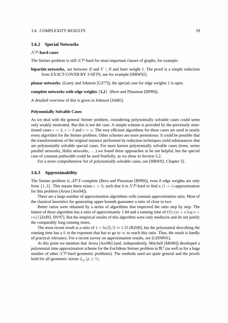
1.6.2 Special Networks
NP-hard cases
The Steiner problem is still NP-hard for most important classes of graphs, for example:
bipartite networks, are between R and V \ R and have weight 1. The proof is a simple reductionfrom EXACT-COVER BY 3-SETS, see for example [HRW92].
planar networks (Garey and Johnson [GJ77]), the special case for edge weights 1 is open.
complete networks with edge weights 1,2 (Bern and Plassman [BP89]).
A detailed overview of this is given in Johnson [Joh85].
Polynomially Solvable Cases
As we deal with the general Steiner problem, considering polynomially solvable cases could seemonly weakly motivated. But this is not the case. A simple scheme is provided by the previously men-tioned cases r = 2, r = 3 and r = n. The very efficient algorithms for these cases are used in nearlyevery algorithm for the Steiner problem. Other schemes are more pretentious: It could be possible thatthe transformations of the original instance performed by reduction techniques yield subinstances thatare polynomially solvable special cases. For most known polynomially solvable cases (trees, seriesparallel networks, Halin networks, . . . ) we found these approaches to be not helpful, but the specialcase of constant pathwidth could be used fruitfully, as we show in Section 5.2.
For a more comprehensive list of polynomially solvable cases, see [HRW92, Chapter 5].
1.6.3 Approximability
The Steiner problem is APX -complete (Bern and Plassman [BP89]), even if edge weights are onlyfrom 1, 2. This means there exists ε > 0, such that it is NP-hard to find a (1 + ε)-approximationfor this problem (Arora [Aro94]).
There are a large number of approximation algorithms with constant approximation ratio. Most ofthe classical heuristics for generating upper bounds guarantee a ratio of close to two.
Better ratios were obtained by a series of algorithms that improved the ratio step by step. Thefastest of these algorithm has a ratio of approximately 1.84 and a running time of O(r(m + n log n +rn)) [Zel93, DV97]. But the empirical results of this algorithm were only mediocre and do not justifythe comparably long running times.
The most recent result is a ratio of 1 + ln(3)/2 ≈ 1.55 [RZ00], but the polynomial describing therunning time has a k in the exponent that has to go to ∞ to reach this ratio. Thus, the result is hardlyof practical relevance. For a recent survey on approximation results, see [GHNP01].
At this point we mention that Arora [Aro96] (and, independently, Mitchell [Mit96]) developed apolynomial time approximation scheme for the Euclidean Steiner problem in
2 (as well as for a hugenumber of other NP-hard geometric problems). The methods used are quite general and the proofshold for all geometric norms Lp (p ≥ 1).
Chapter 2
Theoretical and Practical Aspects ofLinear Programming Relaxations for theSteiner Problem
20

2.1. INTRODUCTION 21
2.1 Introduction
This chapter deals with theoretical and practical aspects of linear programming approaches for theSteiner problem. The basic idea is to reformulate the given problem as an integer linear program.Then, the linear relaxation of these reformulation can be solved (or approximated). This is useful, notonly for computing lower bounds, but also as the basis of many empirically successful heuristics forcomputing upper bounds and sophisticated reduction techniques, culminating in an exact algorithm,which achieves very good empirical results.
There are many (mixed) integer programming formulations of the Steiner problem in networks.Although the strength of the corresponding linear relaxation has great impact on the practical effec-tiveness of the algorithms that are based on it, not much was known about the relative quality ofthese relaxations. In Sections 2.3 to 2.8, we compare the linear relaxations of all classical, frequentlycited and some modified or new integer programming formulations of this problem from a theoreticalpoint of view with respect to their optimal values. We present several new results, establishing clearrelations between relaxations, which have often been treated as unrelated or incomparable.
In Section 2.7, we introduce a collection of new relaxations that are stronger than any relaxationwe are aware of, and place the new relaxations into our hierarchy. Further, we show how one relax-ation of the collection can be used in practical algorithms. Except for the flow-balance constraintsintroduced to the Steiner problem by [KM98], this is the first successful attempt to use a relaxationthat is stronger than Wong’s directed cut relaxation (Section 2.3) from 1984 [Won84].
In Section 2.9, we report on our experimental study of some of these relaxations. Their previouslymentioned algorithmic application for upper bound calculation, reduction techniques, and in the exactalgorithm will be explained in detail in the corresponding chapters.
2.2 Additional Definitions for Lower Bounds
Here we recall two reformulations of the Steiner problem from Section 1.5, because they are used insome relaxations. One uses the directed version: Given G = (V,E, c) and R, find a minimum weightarborescence in ~G = (V,A, c) (A := [vi, vj ], [vj , vi] | (vi, vj) ∈ E, c defined accordingly) with aterminal (say z1) as the root that spans Rz1 := R\z1.
The problem can also be stated as finding a degree-constrained minimum spanning tree T0 in amodified network G0 = (V0, E0, c0), produced by adding a new vertex v0 and connecting it throughzero cost edges to all vertices in V \R and to a fixed terminal (say z1). The problem is now equivalentto finding a minimum spanning tree T0 in G0 with the additional restriction that in T0 every vertex inV \R adjacent to v0 must have degree one. For more details on this reformulation, see [BP87, Bea89].Again, a similar directed version for a network ~G0 can be defined, this time by adding zero cost arcs[v0, vi] (for all vi ∈ V \R) and [v0, z1] to ~G.
We introduce some additional definitions that make the notation of linear relaxations easier tounderstand.
A cut in ~G = (V,A, c) (or in G = (V,E, c)) is defined as a partition C = W,W of V(∅ ⊂ W ⊂ V ;V = W ∪W ). We use δ−(W ) to denote the set of arcs [vi, vj ] ∈ A with vi ∈ W andvj ∈ W . For simplicity, we write δ−(vi) instead of δ−(vi). The sets δ+(W ) and, for the undirectedversion, δ(W ) are defined similarly. A cut C = W,W is called a Steiner cut if z1 ∈ W andRz1 ∩ W 6= ∅ (for the undirected version: R ∩ W 6= ∅ and R ∩ W 6= ∅).
In the integer programming formulations we use (binary) variables xij for each arc [vi, vj ] ∈ A(respectively Xij for each edge (vi, vj) ∈ E), indicating whether an arc is part of the solution (xij =

22 CHAPTER 2. ASPECTS OF LINEAR PROGRAMMING RELAXATIONS
1) or not (xij = 0). Thus, the cost of the solution can be calculated by the dot product c · x, where c isthe cost vector. For any B ⊆ A, x(B) is short for
∑
a∈B xa, and A(W ) denotes [vi, vj ] ∈ A|vi, vj ∈W for any W ⊆ V . For example, x(δ−(W )) is short for
∑
[vi,vj ]∈A,vi 6∈W,vj∈W xij .
Let P1 be an integer linear program. The corresponding linear relaxation is denoted by LP1. Thedual of such a relaxation is denoted by DLP1 and a Lagrangian relaxation by LaLP1. The value of anoptimal solution of the integer programming formulation (for given ~G and R), denoted by v(P1), is ofcourse the value of an optimal solution of the corresponding Steiner arborescence problem in ~G. Thus,in this context we are interested in the optimal value v(LP1) of the corresponding linear relaxation,which can differ from v(P1). The notations P1 (or LP1) always denote an integer (or linear) programcorresponding to an arbitrary, but fixed instance (G,R) of the Steiner problem (with G replaced by~G, G0 or ~G0 when appropriate).
For a linear program Px, the identifier x describes the program (see Table 2.1 for further explana-tion of the abbreviations for linear programs).
C cut based Section 2.3.1
F flow based Section 2.3.2
FR common-flow formulation Section 2.7.3
F j1,j2 restricted version of F R (multiple roots) Section 2.7.4
F 2 restricted version of F R (only one root) Section 2.7.4
2T two-terminal formulation Section 2.3.2
T tree based Section 2.4
mT multiple tree based Section 2.6
T0 degree constraint spanning tree based (with v0 vertex) Section 2.4.1~T directed version of T
U undirected version
X + FB with added flow-balance constraints Section 2.6.2
X− weaker version of X
X + + aggregated version of X
X ′ modified version of X
Table 2.1: Abbreviations for linear programs and their meaning.
We compare relaxations using the predicates equivalent and (strictly) stronger: We call a relax-ation R1 stronger than a relaxation R2 if the optimal value of R1 is no less than that of R2 for allinstances of the problem. If R2 is also stronger than R1, we call them equivalent, otherwise we saythat R1 is strictly stronger than R2. If neither is stronger than the other, they are incomparable.
2.3 Cut and Flow Formulations
In this section, we state the basic flow and cut-based formulations of the Steiner problem. There aresome well-known observations concerning these formulations, which we cite without proof.

2.3. CUT AND FLOW FORMULATIONS 23
2.3.1 Cut Formulations
The directed cut (or dicut) formulation was stated in [Won84].
PC c · x → min,
x(δ−(W )) ≥ 1 (z1 6∈ W,R ∩ W 6= ∅), (1.1)
x ∈ 0, 1|A|. (1.2)
The constraints (1.1) are called Steiner cut constraints. They guarantee that in any arc set correspond-ing to a feasible solution, there is a path from z1 to any other terminal.
A formulation for the undirected version was stated in [Ane80]:
PUC c · X → min,
X(δ(W )) ≥ 1 (W ∩ R 6= R, W ∩ R 6= ∅), (2.1)
X ∈ 0, 1|E|. (2.2)
Lemma 3 LPC is strictly stronger than LPUC ; and sup
v(LPC )v(LPUC)
= 2 [CR94a, Dui93].
We just mention here that v(PUC )v(LPUC ) ≤ 2 [GB93]; and that when applied to undirected instances,
the value v(LPC) is independent of the choice of the root [GM93]. For much more information onLPC , LPUC and their relationship, see [CR94a]. Also, many related results are discussed in [MW95].
2.3.2 Flow Formulations
Viewing the Steiner problem as a multicommodity flow problem leads to the following formulation(see [Won84]).
PF c · x → min,
yt(δ−(vi)) = yt(δ+(vi)) −
1 (zt ∈ Rz1 ; vi = zt),0 (zt ∈ Rz1 ; vi ∈ V \ z1, zt), (3.1)
yt ≤ x (zt ∈ Rz1), (3.2)
yt ≥ 0 (zt ∈ Rz1), (3.3)
x ∈ 0, 1|A|. (3.4)
Each variable ytij denotes the quantity of the commodity t flowing through [vi, vj ]. Constraints (3.1)
guarantee that for each terminal zt ∈ Rz1 , there is a flow of one unit of commodity t from z1 to zt.Together with (3.2), they guarantee that in any arc set corresponding to a feasible solution, there is apath from z1 to any other terminal.
Lemma 4 LPC is equivalent to LPF [Won84].
The correspondence is even stronger: Every feasible solution x for LPC corresponds to a feasiblesolution (x, y) for LPF .
The straightforward translation of PF for the undirected version leads to LPUF with v(LPUF ) =v(LPUC) (see [GM93]). There are other undirected formulations (see [GM93]), leading to relaxationsthat are all equivalent to LPF ; so we use the notation LPFU for all of them.

24 CHAPTER 2. ASPECTS OF LINEAR PROGRAMMING RELAXATIONS
Of course, there is no need for different commodities in PF . In an aggregated version, which wecall PF++, one unit of a single commodity flows from z1 to each terminal zt ∈ Rz1 (see [Mac87]).This program has only Θ(a) variables and constraints, which is asymptotically minimal. But thecorresponding linear relaxation LPF++ is not a strong one:
PF++ c · x → min,
Y (δ−(vi)) = Y (δ+(vi)) −
1 (vi ∈ Rz1),0 (vi ∈ V \ R),
(4.1)
(r − 1)x ≥ Y, (4.2)
Y ≥ 0, (4.3)
x ∈ 0, 1|A|. (4.4)
The variables Y describe a flow of one unit from z1 to each terminal in Rz1 .
Lemma 5 LPF is strictly stronger than LPF++. The worst-case ratio v(LPF )v(LPF++) is r − 1 [Mac87,
Dui93].
In [Liu90], the two-terminal formulation was stated:
P2T c · x → min,
ykl(δ−(vi)) − ykl(δ+(vi)) ≥
−1 (zk, zl ⊆ Rz1 ; vi = z1),0 (zk, zl ⊆ Rz1 ; vi ∈ V \ z1),
(5.1)
(ykl + ykl)(δ−(vi)) − (ykl + ykl)(δ+(vi)) =
1 (zk, zl ⊆ Rz1 ; vi = zk),0 (zk, zl ⊆ Rz1 ; vi ∈ V \ z1, zk),
(5.2)
(ykl + ykl)(δ−(vi)) − (ykl + ykl)(δ+(vi)) =
1 (zk, zl ⊆ Rz1 ; vi = zl),0 (zk, zl ⊆ Rz1 ; vi ∈ V \ z1, zl),
(5.3)
ykl + ykl + ykl ≤ x (zk, zl ⊆ Rz1), (5.4)
ykl, ykl, ykl ≥ 0 (zk, zl ⊆ Rz1), (5.5)
x ∈ 0, 1|A|. (5.6)
The formulation PF is based on the flow formulation of the shortest path problem (the special case ofthe Steiner problem with |Rz1 | = 1). The formulation P2T is based on the special case with |Rz1 | = 2,namely the two-terminal (2T) Steiner arborescence problem. In a Steiner tree, for any two terminalszk, zl ∈ Rz1 , there is a two-terminal tree consisting of a path from z1 to a splitter node vs and twopaths from vs to zk and zl (vs can belong to z1, zk, zl). In P2T , y, y and y describe flows from z1
to vs, from vs to zk and from vs to zl. Note that the flow described by y can have an excess at somevertices (because of the inequality in (5.1)), this excess is carried by the flows described by y and y tozk and zl (because of (5.2) and (5.3)).
Lemma 6 LP2T is strictly stronger than LPF [Liu90].
2.4 Tree FormulationsIn this section, we state the basic tree-based formulations and prove that the corresponding linearrelaxations are all equivalent. We also discuss some variants from the literature, which we prove to beweaker.

2.4. TREE FORMULATIONS 25
2.4.1 Degree-Constrained Tree Formulations
In [Bea89], the following program was suggested, which is a translation of the degree-constrainedminimum spanning tree problem in G0.
PT0c · X → min,
(vi, vj) | Xij = 1 : builds a spanning tree for G0, (6.1)
X0k + Xki ≤ 1 (vk ∈ V \R ; (vk, vi) ∈ δ(vk)), (6.2)
X ∈ 0, 1|E0 |. (6.3)
The requirement (6.1) can be stated by linear constraints. In the following, we assume that (6.1) isreplaced by the following constraints.
X(E0) = n, (6.4)
X(E0(W )) ≤ |W | − 1 (∅ 6= W ⊂ V0). (6.5)
The constraints (6.4) and (6.5), together with the nonnegativity of X , define a polyhedron whoseextreme points are the incidence vectors of spanning trees in G0 (see [Edm71, MW95]). Thus, noother set of linear constraints replacing (6.1) can lead to a stronger linear relaxation.
A directed version can be stated as follows.
P~T0c · x → min,
x(δ−(vi)) = 1 (vi ∈ V ), (7.1)
x(A0(W )) ≤ |W | − 1 (∅ 6= W ⊆ V0), (7.2)
x0i + xij + xji ≤ 1 (vi ∈ V \ R ; [vi, vj ] ∈ δ+(vi) ), (7.3)
x ∈ 0, 1|A0 |. (7.4)
Again, the constraints (7.1) and (7.2), together with the nonnegativity of x, define a polyhedron whoseextreme points are the incidence vectors of spanning arborescences with root v0 (see [MW95]). Notethat δ−(v0) = ∅ by the construction of ~G0.
In the literature on the Steiner problem, one usually finds a directed variant P ~T0−that uses
x0i + xij ≤ 1 (vi ∈ V \ R ; [vi, vj ] ∈ δ+(vi) )
instead of the constraints (7.3) (see for example [HRW92]). Obviously v(P ~T0−) = v(P~T0
), andv(LP~T0−
) ≤ v(LP~T0). The following example shows that LP ~T0
is strictly stronger than the versionin the literature.
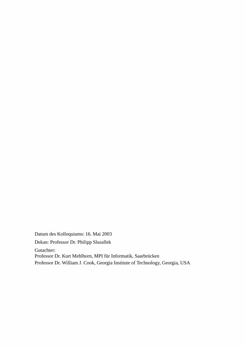
Example 1 Figure 2.1 shows the network ~G with R = z1, z2, γ ≥ 100 and the network ~G0. Theminimum Steiner arborescence has the value γ + 10.The following x is feasible (and optimal) for LP ~T0−
and gives the value 11: x01 = 1, x03 = x04 =
x34 = x43 = x32 = x42 = 12 and xij = 0 (for all other arcs). But for LP ~T0
, x is infeasible. Theoptimal value here is: v(LP ~T0
) = γ3 +14 (this value is reached for example by x with x01 = 1, x03 =
x04 = x13 = x23 = x32 = 13 , x42 = x34 = 2
3 and xij = 0 (for all other arcs)). So the ratiov(LP~T0−
)/v(LP~T0) can be arbitrarily close to 0.

26 CHAPTER 2. ASPECTS OF LINEAR PROGRAMMING RELAXATIONS
| |
l
l
l@
@@
@
@@
@@@@
@@
@@
@@
1z1v0
0
0
0
10
10γ
γ
z2
v3
v4
Figure 2.1: Example with v(LP ~T0−) v(LP~T0
) = v(LPT0) v(PT0
).
2.4.2 Rooted Tree Formulation
The rooted tree formulation is stated, for example, in [KPH93]:
P~Tc · x → min,
x(δ−(vi)) = 1 (vi ∈ Rz1), (8.1)
x(δ−(vi) \ [vj , vi]) ≥ xij (vi ∈ V \ R ; [vi, vj ] ∈ δ+(vi)), (8.2)
x(A(W )) ≤ |W | − 1 (∅ 6= W ⊆ V ), (8.3)
x ∈ 0, 1|A|. (8.4)
To get rid of the exponential number of constraints for avoiding cycles, many authors have consideredreplacing (8.3) by the subtour elimination constraints introduced in the TSP-context (known as theMiller-Tucker-Zemlin constraints [MTZ60]), allowing additional variables ti for all vi ∈ V :
ti − tj + nxij ≤ n − 1 ([vi, vj ] ∈ A). (8.5)
This leads to the program P ~T− with Θ(a) variables and constraints, which is asymptotically minimal.The linear relaxation LP ~T− was used by [KP95]. We will now prove the intuitive guess that LP ~T
is
stronger than LP~T−. Indeed, the ratio
v(LP~T−)
v(LP~T) can be arbitrarily close to 0 (see Figure 2.2 on page
30).
Lemma 7 v(LP~T−) ≤ v(LP~T
).
Proof: Let x denote an (optimal) solution for LP ~T. Obviously x satisfies the constraints (8.1) and
(8.2). We now show that it is possible to construct t such that (x, t) satisfies (8.5), too.We start with an arbitrary t (e.g., ti = 0 (for all vi ∈ V )). We define for every arc [vi, vj ] ∈ A:sij := (n − 1) − (ti − tj + nxij); and call an arc [vi, vj ] good, if sij ≥ 0; used, if sij ≤ 0; and bad,if sij < 0. Suppose [vi, vj ] is a bad arc (if no bad arcs exist, (x, t) satisfies (8.5)).We now show how tj (and perhaps some other tp) can be increased in a way that [vi, vj ] becomesgood, but no good arc becomes bad. By repeating this procedure we can make all arcs good and provethe lemma.In each step we denote by Wj the set of vertices vk ∈ V that can be reached from vj through pathswith only used arcs. We define ∆ as minskl | [vk, vl] ∈ δ+(Wj), if this set is nonempty, and∞ otherwise. Now we increase for all vertices vp ∈ Wj the variables tp by min−sij,∆ (thesevalues can change in every step). By doing this, no arc of δ+(Wj) becomes bad. For arcs [vp, vq] withvp, vq ∈ Wj or vp, vq 6∈ Wj the value of spq does not change; and for arcs [vq, vp] ∈ δ−(Wj) sqp does

2.4. TREE FORMULATIONS 27
not decrease.Because tj is increased in every step, there is only one situation that could prevent that [vi, vj ] becomesgood: In one step vi is absorbed by Wj . But then, according to the definition of Wj , there exists a pathvj ; vi with only used arcs. Thus, there exists a cycle C := (vi, vj = vk1
, . . . , vkl= vi), with
sklk1< 0 and skt−1kt ≤ 0 (for all t ∈ 2, . . . , l). Summation of the inequalities for arcs on the cycle
C leads to: nx(C) > l(n−1). On the other hand, since x satisfies the constraints (8.3), x(C) ≤ l−1.The consequence, l−1
l> n−1
n, is a contradiction. 2
2.4.3 Equivalence of Tree-Class Relaxations
We now show the equivalence of the tree-based relaxations LPT0, LP~T0
, and LP~T.
Lemma 8 v(LP~T0) = v(LPT0
).
Proof:I) v(LP~T0
) ≥ v(LPT0): Let x denote an (optimal) solution for LP ~T0
. Define X with Xij := xij +xji
(for all (vi, vj) ∈ E), X0i := x0i (for all vi ∈ V \ R) and X01 := x01. It is easy to check that Xsatisfies all constraints of LPT0
and yields the same value as v(LP ~T0).
II) v(LPT0) ≥ v(LP~T0
): Now let X denote an (optimal) solution for LPT0. Define ∆ with ∆ij ∈ [0, 1]
arbitrarily (for all (vi, vj) ∈ E) and set x to xij := ∆ijXij , xji := (1−∆ij)Xij (for all (vi, vj) ∈ E),x0i := X0i (for all vi ∈ V \ R) and x01 := X01. Again, it is easy to validate that x satisfies theconstraints (7.2) and (7.3) and yields the same value as v(LPT0
).The only question is, whether there is a ∆ such that x satisfies the constraints (7.1), too. This questioncan be stated in the following way:Is it possible to distribute the “supply” Xij of each edge (vi, vj) in such a way to its end-vertices thatevery vertex vi ∈ V gets one unit at the end?It is known that this problem can be viewed as a flow problem: Construct a flow network with sources, sink t, and vertices uij (for all (vi, vj) ∈ E0) and ui (for all vi ∈ V0). Every uij is connected withui and uj through arcs [uij , ui] and [uij , uj ] with capacity ∞. Furthermore, there are arcs [s, uij ] withcapacity Xij and arcs [ui, t] with capacity 1 (or 0, if i = 0). The question above is equivalent to thequestion, whether a flow from s to t with value n can be constructed. The max-flow min-cut theoremsays that this is possible if and only if there is no cut C = U,U (with s ∈ U and t 6∈ U ) withcapacity less than n (Obviously U = s and U = V \t correspond to cuts with capacity n).Suppose that U corresponds to a cut C with minimum capacity. Define W := vi ∈ V0 | ui ∈ U,EW := (vi, vj) ∈ E0 | vi, vj ∈ W, and EU := (vi, vj) ∈ E0 | uij ∈ U. For every [vi, vj] ∈ EU
(uij ∈ U), ui and uj must belong to U ([vi, vj ] ∈ EW ), because otherwise the capacity of C wouldbe ∞, which is not minimal. It follows that: EU ⊆ EW .The capacity of C is:
|W \ v0| + X(E0 \ EU ) ≥ |W \ v0| + X(E0 \ EW ) (since EU ⊆ EW )
≥ |W | − 1 + X(E0) − X(EW )
= |W | − 1 + n − X(EW ) (because of 6.4)
≥ n. (because of 6.5)
It follows that the minimal cut has capacity of n. 2
Lemma 9 v(LP~T) = v(LP~T0
).

28 CHAPTER 2. ASPECTS OF LINEAR PROGRAMMING RELAXATIONS
Proof:I) v(LP~T0
) ≥ v(LP~T): Let x denote an (optimal) solution for LP ~T0
. Define x with xij := xij (for
all [vi, vj ] ∈ A). Because x satisfies the constraints (7.1) and in ~G0 only arcs in A are incident withterminals in Rz1 , x satisfies the constraints (8.1).Furthermore, x satisfies the constraints (8.2), because for every arc [vi, vj ] ∈ A with vi ∈ V \ R itholds that:
x(δ−(vi) \ [vj , vi]) = x(δ−(vi)) − xji (δ in ~G)
= x(δ−(vi)) − x0i − xji (δ in ~G0)
= 1 − x0i − xji (because of (7.1) )
≥ xij (because of (7.3) )
= xij.
Finally x satisfies (8.3), because x satisfies (7.2).II) v(LP~T
) ≥ v(LP~T0): Let x denote an (optimal) solution for LP ~T
. Define x with xij := xij (forall [vi, vj ] ∈ A) and x0i := 1 − x(δ−(vi)) (for all vi ∈ V \ Rz1). Notice that for an optimal x,x(δ−(vi)) > 1 could only be forced by (8.2) for some arc [vi, vl] with x(δ−(vi) \ [vj , vi]) = xil,and it would follow that 1 < x(δ−(vi)) = xli + xil, but this is excluded by (8.3) (for W = vi, vl).So x satisfies (7.1) in a trivial way.The constraints (7.2) are satisfied by x for every W ⊆ V , because x satisfies (8.3). For W ⊆ V0 withv0 ∈ W it holds that:
x(A0(W )) ≤∑
vi∈W\v0
x(δ−(vi)) (in ~G0)
=∑
vi∈W\v0
1 (because of (7.1) )
= |W | − 1.
Finally for every [vi, vj ] ∈ A with vi ∈ V \ R:
x0i + xij + xji = 1 − x(δ−(vi)) + xij + xji (in ~G)
= 1 − x(δ−(vi) \ [vj , vi]) + xij
≤ 1. (because of (8.2) )
Thus, x also satisfies the constraints (7.3). 2
2.5 Relationship between the Two Classes
In this section, we settle the question of the relationship between flow and tree-based relaxations byproving that LPC is strictly stronger than LP ~T
. Our proofs also show that LPC cannot be strengthenedby adding constraints that are present in LP ~T0
or LP~T.
First, we show that every (optimal) solution x of LPC has certain properties:
Lemma 10 For every (optimal) solution x of LPC , W ⊆ V \z1 and vk ∈ W the following holds:
x(δ−(W )) ≥ x(δ−(vk)).

2.5. RELATIONSHIP BETWEEN THE TWO CLASSES 29
Proof: Suppose that x violates the inequality for some W and vk. Among all such inequalities,choose one for which |W | is minimal. For this inequality to be violated, there must be an arc[vl, vk] ∈ δ−(vk)\δ−(W ) with xlk > 0. Because of the optimality of x, xlk cannot be decreased with-out violating a Steiner cut constraint, so there is a U ⊂ V with z1 /∈ U, U ∩R 6= ∅, [vl, vk] ∈ δ−(U),and x(δ−(U)) = 1. Now one has the inequality †:
x(δ−(U)) + x(δ−(W )) = x(δ−(U ∪ W )) + x(δ−(U ∩ W )) +
x([vi, vj ] ∈ A | vi ∈ W\U, vj ∈ U\W ) +
x([vj , vi] ∈ A | vi ∈ W\U, vj ∈ U\W )
≥ x(δ−(U ∪ W )) + x(δ−(U ∩ W ))
Since z1 /∈ U ∪W and (U ∪W )∩R 6= ∅, U ∪W corresponds to a Steiner cut, and x(δ−(U ∪W )) ≥1 = x(δ−(U)). Using †, one obtains: x(δ−(W )) ≥ x(δ−(U ∩ W )). This implies that x also violatesthe lemma for U ∩ W and vk. Since vl ∈ W\U , we have |U ∩ W | < |W |, and this contradicts theminimality of W .1 2
Lemma 11 For every (optimal) solution x of LPC and vk ∈ V \z1 the following holds:
x(δ−(vk)) ≤ 1.
Proof: Suppose x violates the inequality for vk. There is an arc [vl, vk] ∈ δ−(vk) with xlk > 0.Because of the optimality of x, xlk cannot be decreased without violating a Steiner cut constraint, sothere is a W ⊂ V with z1 /∈ W, W ∩ R 6= ∅, [vl, vk] ∈ δ−(W ), and x(δ−(W )) = 1. Together withLemma 10 (for vk and W ), one gets a contradiction. 2
Lemma 12 For every (optimal) solution x of LPC , vl ∈ V \z1, and [vl, vk] ∈ A the followingholds:
x(δ−(vl) \ [vk, vl]) ≥ xlk.
Proof: This follows directly from Lemma 10 (for vk and W = vl, vk) by subtracting x(δ−(vl) \[vk, vl]) from both sides. Note that the special case vk = z1 is trivial, because xl1 = 0 in everyoptimal solution. 2
Theorem 13 v(LP~T) ≤ v(LPC).
Proof: Let x be an (optimal) solution for LPC . We will show that x is feasible for LP ~T:
Because vi corresponds to a Steiner cut for vi ∈ Rz1 , through the use of Lemma 11, x satisfies(8.1).Because of Lemma 12, x satisfies (8.2).Let W ⊆ V be a nonempty set. If z1 ∈ W :
x(A(W )) ≤∑
vi∈W
x(δ−(vi))
=∑
vi∈W\z1
x(δ−(vi)) (optimality of x)
≤∑
vi∈W\z1
1 (Lemma 11)
= |W | − 1.1In a different context this argumentation was used in [GM93].

30 CHAPTER 2. ASPECTS OF LINEAR PROGRAMMING RELAXATIONS
Now we assume z1 6∈ W and define ∆ := x(δ−(W )). There are two cases:I) ∆ ≥ 1 :
x(A(W )) =∑
vi∈W
x(δ−(vi)) − x(δ−(W ))
≤∑
vi∈W
x(δ−(vi)) − 1 (∆ ≥ 1)
≤∑
vi∈W
1 − 1 (Lemma 11)
= |W | − 1.
II) ∆ < 1 :
x(A(W )) =∑
vi∈W
x(δ−(vi)) − x(δ−(W ))
≤∑
vi∈W
x(δ−(W )) − x(δ−(W )) (Lemma 10)
= (|W | − 1)x(δ−(W ))
< |W | − 1. (∆ < 1)
It follows that x satisfies (8.3) too. 2
Corollary 13.1 The proof shows that adding constraints of LP ~Tto LPC cannot improve v(LPC).
Corollary 13.2 Because the proofs of the equivalence of the tree relaxations require the optimalityonly in one step of Lemma 9 to show that x(δ−(vi)) ≤ 1, which is forced by Lemma 11 for each(optimal) solution of LPC , adding constraints of LP ~T0
to LPC cannot improve v(LPC) either.
To show that LPF and LPC are strictly stronger than the tree-based relaxations LPT0, LP~T0
, andLP~T
, it is sufficient to give the following example.
1 1
| |l l
l l@
@@
@
@@
@@
z2
v3
z1
v4
v5 v6
α α
α
1
γ
Figure 2.2: Example for v(LP ~T−) v(LP~T) v(LPF ) = v(PF ).
Example 2 For the network G (or in the directed view ~G) in Figure 2.2 set α 1 and γ α.Obviously, v(PF ) = v(LPF ) = γ. For LP~T
is x with x23 = x34 = x42 = 23 , x25 = x56 = x62 = 1
3 ,and xij = 0 (otherwise) feasible, even optimal, and gives the value v(LP ~T
) = α + 2. Thus, there is

2.6. MULTIPLE TREES AND THE RELATION TO THE FLOW MODEL 31
no positive lower bound for the ratiov(LP~T
)
v(LPF ) .
With respect to LP~T− and LP~T, one observes that (x, t) with ti = 0 (for all vi ∈ V ), x23 = x32 =
x34 = x43 = x24 = x42 = 12 , and xij = 0 (otherwise) is an (optimal) solution for LP ~T− with the
value 3. So, there is no positive lower bound for the ratiov(LP~T−
)
v(LP~T) .
2.6 Multiple Trees and the Relation to the Flow Model
In this section, we consider a relaxation based on multiple trees and prove its equivalence to an aug-mented flow relaxation. We also discuss some variants of the former relaxation.
2.6.1 Multiple Trees Formulation
In [KPH93], a variant of P ~Twas stated, using the idea that an undirected Steiner tree can be viewed
as |R| different Steiner arborescences with different roots.
Pm~T
c · X → min,
X(δ(vi)) ≥ 1 (vi ∈ R), (9.1)
X(δ(vi)) ≥ 2si (vi ∈ V \ R), (9.2)
si ≥ Xij (vi ∈ V \ R ; (vi, vj) ∈ δ(vi) ), (9.3)
xkij + xk
ji = Xij (vk ∈ R ; (vi, vj) ∈ E), (9.4)
xk(δ−(vi)) =
1 (vk ∈ R ; vi ∈ R \ vk),0 (vk ∈ R ; vi = vk),
(9.5)
xk(δ−(vi)) = si (vk ∈ R ; vi ∈ V \ R), (9.6)
[vi, vj ] | xkij = 1 : contains no cycles (vk ∈ R), (9.7)
X ∈ 0, 1|E|, (9.8)
xk ∈ 0, 1|A| (vk ∈ R), (9.9)
si ∈ 0, 1 (vi ∈ V \ R). (9.10)
In any feasible solution for Pm~T
, each group of variables xk describes an arborescence (with root zk)spanning all terminals. The variables s describe the set of the other vertices used by these arbores-cences.
We will relate this formulation to the flow formulations. First, we have to present an improvementof LPF .
2.6.2 Flow-Balance Constraints and an Augmented Flow Formulation
There is a group of constraints (see for example [KM98]) that can be used to make LPF stronger. Wecall them flow-balance constraints:
x(δ−(vi)) ≤ x(δ+(vi)) (vi ∈ V \ R). (10.1)
We denote the linear program that consists of LPF and (10.1) by LPF+FB . It is obvious that LPF+FB
is stronger than LPF . The following example shows that it is even strictly stronger.
32 CHAPTER 2. ASPECTS OF LINEAR PROGRAMMING RELAXATIONS
| |
| l
l
@@
@@
@
z1
z3
z2
s1
s2
3
3
1
11
1
1
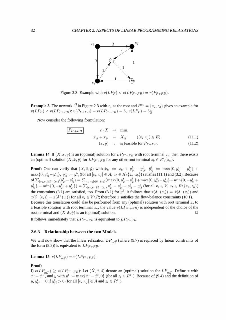
Figure 2.3: Example with v(LPF ) < v(LPF+FB) = v(PF+FB).
Example 3 The network ~G in Figure 2.3 with z1 as the root and Rz1 = z2, z3 gives an example forv(LPF ) < v(LPF+FB): v(PF+FB) = v(LPF+FB) = 6, v(LPF ) = 51
2 .
Now consider the following formulation:
PF ′+FB c · X → min,
xij + xji = Xij ((vi, vj) ∈ E), (11.1)
(x, y) : is feasible for PF+FB . (11.2)
Lemma 14 If (X,x, y) is an (optimal) solution for LPF ′+FB with root terminal za, then there existsan (optimal) solution (X, x, y) for LPF ′+FB for any other root terminal zb ∈ R\za.
Proof: One can verify that (X, x, y) with xij := xij + ybji − yb
ij, ytij := max0, yt
ij − ybij +
max0, ybji−yt
ji, yaij := yb
ji (for all [vi, vj ] ∈ A, zt ∈ R\za, zb) satisfies (11.1) and (3.2). Becauseof
∑
[vj ,vi]∈δ−(vi)(ytji− yt
ij) =∑
[vj ,vi]∈δ−(vi)(max0, ytji−yb
ji+max0, ybij −yt
ij+min0,−ytij +
ybij + min0,−yb
ji + ytji) =
∑
[vj ,vi]∈δ−(vi) ytji − yb
ji + ybij − yt
ij (for all vi ∈ V, zt ∈ R\za, zb)
the constraints (3.1) are satisfied, too. From (3.1) for yb, it follows that x(δ−(vi)) = x(δ−(vi)) andx(δ+(vi)) = x(δ+(vi)) for all vi ∈ V \R; therefore x satisfies the flow-balance constraints (10.1).Because this translation could also be performed from any (optimal) solution with root terminal zb toa feasible solution with root terminal za, the value v(LPF ′+FB) is independent of the choice of theroot terminal and (X, x, y) is an (optimal) solution. 2
It follows immediately that LPF ′+FB is equivalent to LPF+FB .
2.6.3 Relationship between the two Models
We will now show that the linear relaxation LPm~T
(where (9.7) is replaced by linear constraints ofthe form (8.3)) is equivalent to LPF+FB .
Lemma 15 v(LPm~T
) = v(LPF ′+FB).
Proof:I) v(LP
m~T) ≥ v(LPF ′+FB): Let (X, x, s) denote an (optimal) solution for LP
m~T. Define x with
x := x1 , and y with yt := maxx1 − xt, 0 (for all zt ∈ Rz1 ). Because of (9.4) and the definition ofy, yt
ij = 0 if ytji > 0 (for all [vi, vj ] ∈ A and zt ∈ Rz1).

2.7. A COLLECTION OF NEW FORMULATIONS 33
For all zt ∈ Rz1 , vi ∈ V \z1, zt it holds that:
yt(δ−(vi)) − yt(δ+(vi)) = (x1 − xt)([vj , vi] ∈ δ−(vi)|x1ji > xt
ji) −(x1 − xt)([vi, vj ] ∈ δ+(vi)|x1
ij > xtij)
= (x1 − xt)([vj , vi] ∈ δ−(vi)|x1ji > xt
ji) +
(x1 − xt)([vj , vi] ∈ δ−(vi)|x1ji < xt
ji) (because of (9.4) )
= (x1 − xt)(δ−(vi)) = 0 (because of (9.5) or (9.6) ).
With the same argumentation adapted to vi = zt, it follows that y satisfies (3.1).The other constraints (3.2) are satisfied in a trivial way. A substitution of (9.4) and (9.6) into (9.2)gives the flow-balance constraints (10.1). Thus, (X,x, y) is feasible for LPF ′+FB .II) v(LP
m~T) ≤ v(LPF ′+FB): Let (X,x, y) denote an (optimal) solution for LPF ′+FB . From lemma
14 we know that there is an (optimal) solution (X, xr, yr) for each choice of the root vertex zr ∈ R,with the property that si := xt(δ−(vi)) (for any vi ∈ V \R) has the same value for any choice ofzt ∈ R. With the argumentation of Theorem 13 it follows that (X, x, s) is feasible for LP
m~T. 2
Corollary 15.1 The constraints (9.1), (9.3), and (9.7) are useless with respect to the value of the linearrelaxation LP
m~T.
Corollary 15.2 The linear program LPm~T−(with the same objective function as LP
m~T) that contains
only the equations (9.4), (9.5), and (9.6) is equivalent to LPF .
2.7 A Collection Of New Formulations
In [PV01a] we introduced the common flow formulation LPF 2 , the strongest linear relaxation of poly-nomial size known so far. Concerning this relaxation we have frequently been asked three questions:How we developed the new relaxation, whether the result can be strengthened (the notation LPF 2
looks as if there could be an LPF 3 ) and how a relaxation of this kind could be used in a practicalalgorithm. We will address all three issues in the following.
2.7.1 Properties of the Flow/Cut Relaxations
z1
2 2
1 1
2 2
22 1
4
z2z
3
76 vv v
v5
Figure 2.4: Example with v(LPC) < v(PC).

34 CHAPTER 2. ASPECTS OF LINEAR PROGRAMMING RELAXATIONS
A network with a deviation between the integral and the linear solution is shown in Figure 2.4.Choosing z1 as root yields the value 7.5 as v(LPF ) (setting all x-variables in the direction away fromz1 to 0.5 leads to an optimal solution), while an optimal Steiner tree (and v(PF )) has value 8. Thusthe integrality gap is at least 8
7.5 .Goemans [Goe98] extends the example in Figure 2.4 and constructs networks Gk whose in-
tegrality gap comes arbitraily close to 87 . The network Gk consists essentially of
(k2
)
copiesof the network in Figure 2.4. It has k + 1 terminals a0, a1, ..., ak , and k2 non-terminalsb1, ..., bk , c12, ..., cij , ..., ck−1,k, d12, ..., dij , ..., dk−1,k . For any i and j, 1 ≤ i < j ≤ k one includesthe network of Figure 2.4 with the following labeling: z1 is a0, z2 is ai, z3 is aj , v4 and v5 are cij
and dij , and v6 and v7 are bi and bj . An optimal Steiner tree has value 4k and the optimal LPC so-lution is obtained by setting all x-variables in the direction away from a0 to 1
k, yielding the value
1k(4k + 7
(k2
)
) = 3.5k + 0.5. Thus, the integrality gap approaches 87 with increasing k. This is the
largest integrality gap known2.
z1
4
z2z
3
76 vv v
v5
z1
4
z2z
3
76 vv v
v5
z1
4
z2z
3
76 vv v
v5
z1
4
z2z
3
76 vv v
v5
Figure 2.5: y-variables and decomposition into trees.
Figure 2.5 shows how the y-variables of the LPF solution for Figure 2.4 can be viewed as alinear combination of incidence vectors of paths in some trees. The upper-left network shows the y 2
variables, each arc [vi, vj ] corresponds to y2ij = 0.5. The upper-right figure shows the same for y3.
The y values can be decomposed into two rooted trees T1 and T2 that are depicted in the two figuresat the bottom. For any zt ∈ Rz1 , yt is a linear combination of the incidence vectors of the paths from
2Independently, we constructed other examples with the same asymptotic integrality gap. For example, the edges be-tween ai and bi can be deleted for every i without deteriorating the asymptotic result.

2.7. A COLLECTION OF NEW FORMULATIONS 35
z1 to zt in T1 and T2 (in this example both incidence vectors have weight 0.5).If the x-variables were a linear combination of the incidence vectors of these trees, the optimal
value of the linear relaxation would be the same as of the integral formulation. In this example, wesee that the arc [v4, v5] causes the problem: The linear combination of the incidence vectors of thetrees yields 1 for [v4, v5], while x45 has the value 0.5. Looking at the flow-variables y2 and y3 one cansee that at vertex v4 flows of the different commodities enter from different arcs (y2
74 = y364 = 0.5),
but depart together on arc [v4, v5]. We denote this situation as a rejoining. Formally, a rejoining offlows of the commodities zi1 , zi2 , . . . , zik =: B at vertex vi ∈ V is defined by the condition∑
e∈δ−(vi) max yte|zt ∈ B >
∑
e∈δ+(vi) max yte|zt ∈ B. In Section 2.7.3 we will show how to
attack rejoining of flow in an extended linear program.This situation is typical. In fact, we do not know of any example for a network with an integrality
gap for LPC that does not include a variant of Figure 2.4. Of course, there may be additional edges,edges replaced by paths, other edge weights and non-terminals replaced by terminals, but still Fig-ure 2.4 is a minor of the network (a minor is a subgraph obtained after a sequence of contractionsand deletions, for the relation of minors to linear relaxations for the Steiner problem see [CR94a]).Furthermore, the rejoining of flows of different commodities is a common property of all examplesknown to us, although more than two flows can rejoin (as we will show in Figure 2.6) and it mayneed a change of the root to see a rejoining. Figure 2.4 can be used to illustrate the latter: Turn v4
into a terminal z4 and choose z4 as root, the optimal linear solution value stays the same (setting allx-variables in the direction away from z4 to 0.5 leads to an optimal solution). Again, the y-variablescan be decomposed into the same trees T1 and T2 (just with a reorientation of the arcs), but now thereis no rejoining of flows.
2.7.2 Common Flow
As we have seen in the last section, the typical problematic situation for LPF can be described as therejoining of flows of different commodities. We capture this condition in linear constraints with thehelp of additional variables yB (for all subsets B ⊆ Rz1) that describe the amount of flow going fromthe root to any terminal zt ∈ B: yB ≥ yt, for all zt ∈ B. From Figure 2.5 it is easy to see the flowto z2 and z3 (yz2,z3) incoming at v4 is greater than the flow outgoing of v4. This cannot be the caseif the x-variables correspond to a feasible Steiner tree. Thus, we can introduce additional constraintsthat assure that for each common flow the outgoing flow at any vertex has at least the value of theincoming flow.3
As already noted in Section 2.7.1, the same network can or cannot have rejoining of flow, depend-ing on the choice of the root. To detect all rejoining we have to consider all possible roots. Thus, thevariables that will be used to describe the common flow formulation will have the shape y r,B and theywill describe a flow from zr to all terminals zt ∈ B ⊆ Rzt (we will skip the chosen root in thenotation if the root is clear from the context).
2.7.3 A Collection of Common Flow Formulations
We will first describe the full common flow formulation that has an exponential number of constraintsand variables, and describe afterwards how to reduce it to different formulations (e.g., of only poly-nomial size)
3In [PV01a] we used a semantically inverse, but mathematically equivalent definition of the common flow. Meanwhile,we find the new definition more intuitive and compact.
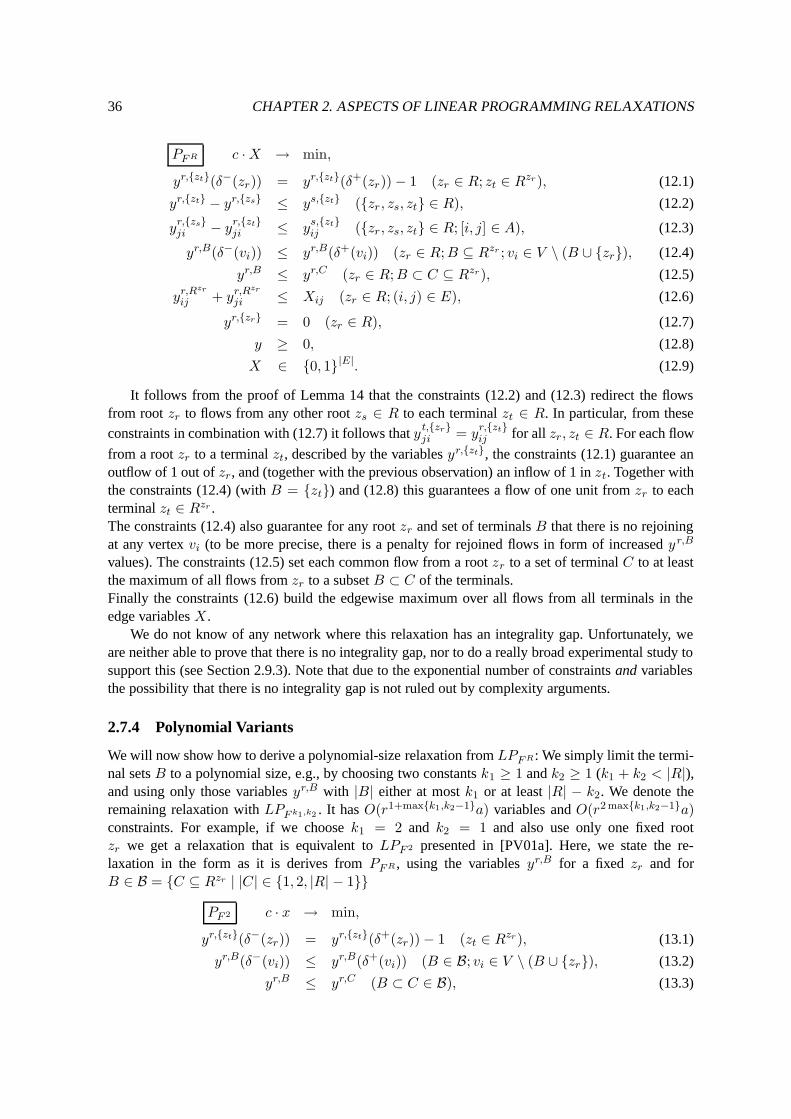
36 CHAPTER 2. ASPECTS OF LINEAR PROGRAMMING RELAXATIONS
PF R c · X → min,
yr,zt(δ−(zr)) = yr,zt(δ+(zr)) − 1 (zr ∈ R; zt ∈ Rzr), (12.1)
yr,zt − yr,zs ≤ ys,zt (zr, zs, zt ∈ R), (12.2)
yr,zsji − y
r,ztji ≤ y
s,ztij (zr, zs, zt ∈ R; [i, j] ∈ A), (12.3)
yr,B(δ−(vi)) ≤ yr,B(δ+(vi)) (zr ∈ R;B ⊆ Rzr ; vi ∈ V \ (B ∪ zr), (12.4)
yr,B ≤ yr,C (zr ∈ R;B ⊂ C ⊆ Rzr), (12.5)
yr,Rzr
ij + yr,Rzr
ji ≤ Xij (zr ∈ R; (i, j) ∈ E), (12.6)
yr,zr = 0 (zr ∈ R), (12.7)
y ≥ 0, (12.8)
X ∈ 0, 1|E|. (12.9)
It follows from the proof of Lemma 14 that the constraints (12.2) and (12.3) redirect the flowsfrom root zr to flows from any other root zs ∈ R to each terminal zt ∈ R. In particular, from theseconstraints in combination with (12.7) it follows that y
t,zrji = y
r,ztij for all zr, zt ∈ R. For each flow
from a root zr to a terminal zt, described by the variables yr,zt, the constraints (12.1) guarantee anoutflow of 1 out of zr, and (together with the previous observation) an inflow of 1 in zt. Together withthe constraints (12.4) (with B = zt) and (12.8) this guarantees a flow of one unit from zr to eachterminal zt ∈ Rzr .The constraints (12.4) also guarantee for any root zr and set of terminals B that there is no rejoiningat any vertex vi (to be more precise, there is a penalty for rejoined flows in form of increased yr,B
values). The constraints (12.5) set each common flow from a root zr to a set of terminal C to at leastthe maximum of all flows from zr to a subset B ⊂ C of the terminals.Finally the constraints (12.6) build the edgewise maximum over all flows from all terminals in theedge variables X .
We do not know of any network where this relaxation has an integrality gap. Unfortunately, weare neither able to prove that there is no integrality gap, nor to do a really broad experimental study tosupport this (see Section 2.9.3). Note that due to the exponential number of constraints and variablesthe possibility that there is no integrality gap is not ruled out by complexity arguments.
2.7.4 Polynomial Variants
We will now show how to derive a polynomial-size relaxation from LPF R : We simply limit the termi-nal sets B to a polynomial size, e.g., by choosing two constants k1 ≥ 1 and k2 ≥ 1 (k1 + k2 < |R|),and using only those variables yr,B with |B| either at most k1 or at least |R| − k2. We denote theremaining relaxation with LPF k1,k2 . It has O(r1+maxk1,k2−1a) variables and O(r2 maxk1,k2−1a)constraints. For example, if we choose k1 = 2 and k2 = 1 and also use only one fixed rootzr we get a relaxation that is equivalent to LPF 2 presented in [PV01a]. Here, we state the re-laxation in the form as it is derives from PF R , using the variables yr,B for a fixed zr and forB ∈ B = C ⊆ Rzr | |C| ∈ 1, 2, |R| − 1
PF 2 c · x → min,
yr,zt(δ−(zr)) = yr,zt(δ+(zr)) − 1 (zt ∈ Rzr), (13.1)
yr,B(δ−(vi)) ≤ yr,B(δ+(vi)) (B ∈ B; vi ∈ V \ (B ∪ zr), (13.2)
yr,B ≤ yr,C (B ⊂ C ∈ B), (13.3)

2.7. A COLLECTION OF NEW FORMULATIONS 37
yr,Rzr= x, (13.4)
y ≥ 0, (13.5)
x ∈ 0, 1|A|. (13.6)
z3 z4
z2z
z5
1
3
1 1
111
3
3 33
3
333
3
33
Figure 2.6: v(LPF ) = 1413 < v(LPF 2,1) = 142
3 < v(LPF R) = 15 = v(PF R).
The drawback of this limitation is that not all rejoinings will be detected by the limited relaxation,as the following example shows: In Figure 2.6, using LPF with z1 as root, there is a rejoining of 3different flows (y2, y3 and y4) at the central vertex. As LPF 2 captures only rejoining of 2 flows, therewill still be some integrality gap. The figure also shows how k2 weakens the relaxation: Only if thecommon flow yr,B to a set of terminals B is considered where z2, z3 and z4 are in B, but z5 is not inB, the relaxation gives the optimal integer value. Thus, for k1 ≥ 3 or k2 ≥ 2 there is no integralitygap.
Note that the example in Figure 2.6 can be generalized to a network G[k1, k2], which produces anintegrality gap for any common flow relaxation that is limited by some constants k1 and k2: Around acenter vertex v0 put k1 + 2 edges [v0, v1], [v0, v2], . . . , [v0, vk1+2] of cost 1. Additionally use k1 + 2terminals (a1, a2, . . . , ak1+2). Each of the terminals zi ∈ R is connected to all vertices vj , j 6= 0, j 6= iwith edges of cost k1+1. Then connect the center vertex to k2 different terminals (b1, b2, . . . , bk2
) withedges of cost 1. An integer optimal solution has the cost k2 + (k1 + 1)(k1 + 2) + 2, but the followingX-variables are feasible for the k1, k2 limited common flow relaxation: Set X-variables of edgesconnected to bi, 1 ≤ i ≤ k2 to 1, the X-variable for (v0, v1) to 1−(k1+1)−1 and all other X variablesto (k1+1)−1. Thus, the optimal value of the relaxation is at most k2+(k1+1)(k1+2)+2−(k1+1)−1.Figure 2.6 shows the network G[2, 1].
As a consequence, we have derived a collection of polynomial relaxations LPF k1,k2 , whereLPF k1,k2 can be related to LPF j1,j2 . We assume that k1 + k2 ≤ j1 + j2.
k1 ≤ j1, k2 ≤ j2: The relaxation LPF j1,j2 is stronger than LPF k1,k2 (since it contains a superset ofthe constraints and variables). If additionally k1 < j1 or k2 < j2, the relaxation LPF j1,j2 iseven strictly stronger. Consider the network G[mink1, j1,mink2, j2], LPF j1,j2 gives theoptimal solution, while LPF k1,k2 has an integrality gap.
otherwise: The relaxations are incomparable. To see this, consider the networksG[mink1, j1,maxk2, j2] and G[maxk1, j1,mink2, j2].
Now, we show why considering all roots is important. The only difference between the relaxationsLPF 2,1 and LPF 2 is that LPF 2,1 considers all terminals as root.

38 CHAPTER 2. ASPECTS OF LINEAR PROGRAMMING RELAXATIONS
Lemma 16 The relaxation LPF 2,1 is strictly stronger than LPF 2 .
Proof: The relaxation LPF 2,1 is stronger than LPF 2 , as it contains a superset of the constraints andvariables. The network G[1, 1] can be used to show that LPF 2,1 is even strictly stronger than LPF 2 .Here, LPF 2,1 gives the optimal value, but for LPF 2 it depends on the choice of the root. Using anyof the vertices a1, a2, or a3 as root gives the integer optimal value, while with b1 as root there is anintegrality gap. 2
2.7.5 Restricted Version
We tested different restricted versions of the common flow relaxation, but did not come to a definitiveconclusion which approach is the best. Nevertheless, we can present a very restricted, but still veryuseful version.
We observed that in many cases the tracing of the common flow to all |R| − 1 terminals (k2 = 1)catches most of the problematic situations except for insightfully constructed pathological instances.As depicted in Figure 2.6, to fool the relaxation with k2 = 1, there typically has to be a terminal di-rectly connected to the vertex at which the rejoining happens. In most of the cases where this happens,the terminal is the vertex itself. To attack those situations without the need to introduce a quadraticnumber of constraints or variables, we restrict the common flow relaxation by k1 = k2 = 1 on non-terminals, and to k2 = 2 on terminals, but only considering the set R \ zr, zi at a terminal zi (withrespect to root zr). Additionally, we restrict the relaxation to one fixed root zr, and because we do notneed the X variables for different roots anymore, we can use the yRzr as x variables.
In a branch-cut-price framework it is highly desirable to introduce as few variables as possible.Working with flow-based relaxations makes this difficult, because if a flow variable on one edge isnecessary, all variables and all flow conservation constraints have to be inserted to get somethinguseful. Therefore the cut-based relaxations are more suitable in this context. In analogy to PC , we canuse constraints of the form y
zi (δ−(W )) ≥ 1 for all W ∩ zr, zi = zi.
Finally, we eliminate all variables yzi and yR\zr ,zie if e is not in δ−(zi) in the following way:
Unwanted yzi variables are replaced by yR\zr ,zi if the replacement is possible using the constraints(12.5). Similarly, unwanted yR\zr ,zi variables are replaced by x if possible. All constraints that stilluse unwanted variables are deleted.
Now, we have the following formulation:
PC′ c · x → min,
x(δ−(W )) ≥ 1 (z1 6∈ W,R ∩ W 6= ∅), (14.1)
yR\zr ,zi(δ−(W ) ∩ δ−(zi)) + x(δ−(W ) \ δ−(zi)) ≥ 1 (zr 6∈ W,Rzi ∩ W 6= ∅), (14.2)
x(δ−(vi)) ≤ x(δ+(vi)) (vi ∈ V \ R), (14.3)
yR\zr ,zi(δ−(zi)) ≤ x(δ+(zi)) (zi ∈ Rzr), (14.4)
y ≥ 0, (14.5)
x ∈ 0, 1|A|. (14.6)
This new formulation has fewer than 2|A| variables. Although it has an exponential number ofconstraints, solving the linear relaxation is relatively easy. This will be described in Section 2.9.3.
2.7.6 Relation to Other Relaxations
Lemma 17 v(LPF 2) ≥ v(LP2T ).

2.7. A COLLECTION OF NEW FORMULATIONS 39
Proof: Let (x, y) be an (optimal) solution of LPF 2 . For all zk, zl ⊆ Rzr and k < l define ykl :=yr,zk − yr,zk,zl, ykl := yr,zl − yr,zk,zl, and ykl := yr,zk,zl. The variables (x, y, y, y) satisfythe constraints of LP2T . 2
Because LPF 2 contains the flow-balance constraints and is stronger than LP2T , it is strongerthan LP2T+FB (constructed by adding (10.1) to LP2T ). It follows directly that LPF 2 is also strongerthan LPF+FB . The following example shows that it is even strictly stronger than the other statedrelaxations.
| |
| l
l|
%%%%%@
@@
@
@@
@@ @
@@
@
z25
1
11
11
1
v6
v5
z3
z4
z1
5
5
6
Figure 2.7: Example with v(LP2T ) < v(LPF+FB) = v(LPF 2) = v(PF 2).
Example 4 Here is an example for v(LP2T ) < v(LPF 2) = v(PF 2): Setting all x-variables to 0.5leads to a feasible (and optimal) solution for LP2T with the value 13.5. An optimal solution forLPF 2 is x13 = x35 = x56 = x62 = x64 = 1, which forms a Steiner tree with value 14. Noticethat this is also an example with v(LP2T ) < v(LPF+FB). On the other hand, if v5 is moved to R,v(LPF+FB) = v(LPF ) = 12 < v(LP2T ) = v(LP2T+FB) = 13.5 < v(LPF 2) = v(PF 2) (Theoptimal value for LPF+FB is reached by x with x12 = x13 = x14 = x25 = x35 = x45 = 1/3, x56 =x62 = x63 = x64 = 2/3). Thus, LPF+FB and LP2T are incomparable.This example has been chosen because it is especially instructive. For v(LP2T+FB) < v(LPF 2), asfor all other statements in this work that one relaxation is strictly stronger than another, we also know(originally) undirected instances as examples.
The relaxation LPF 2 , as well as LP2T , makes it difficult for flows to two different terminals to splitup and rejoin by increasing the x-variables on arcs with rejoined flow. One could say that rejoininghas to be “payed” for. To get an intuitive impression why LPF 2 is strictly stronger than LP2T (or evenLP2T+FB), notice that in LPF 2 , there is one flow to each terminal and rejoining of each pair of theseflows has to be payed for; while in LP2T , it is just required that for each pair of terminals there aretwo flows and rejoining them has to be payed for. The latter task is easier; for example it is possible(for given x-values) that for each pair of terminals there are two flows that do not rejoin, but thereare not |Rz1 | flows to all terminals in Rz1 that do not rejoin pairwise; this is the case in example 2.7(setting all x-variables to 0.5).
Still, we have to prove two more relations to relate the common flow relaxations to the otherrelaxations.
Lemma 18 The relaxation LPF+FB is equivalent to LPF 1,1 .
Proof: The relaxations are nearly the same. The only difference is that LPF 1,1 considers all possibleroots. But as we have seen in Lemma 14, the choice of the root does not change the value of the

40 CHAPTER 2. ASPECTS OF LINEAR PROGRAMMING RELAXATIONS
solution and the transformation of a solution for one root into a solution for another is covered exactlyby the constraints (12.2) and (12.3). 2
Lemma 19 The relaxation LPF 2 is strictly stronger than LPC′ and LPC′ is strictly stronger thanLPF 1,1 .
Proof: It is obvious that LPF 2 is stronger than LPC′ , as LPC′ is a restricted and aggregated version ofLPF 2 . Similarly, LPC′ contains a superset of variables and constraints of LPC+FB , which is equiv-alent to LPF 1,1 . To see that the relations are also strictly stronger, consider the networks G[1, 1]. Ifwe choose a1, a2, or a3 as root, LPC′ has an integrality gap, LPF 2 not. And if we contract the edge(v0, b1), LPC′ gives the integer optimal value, while LPF 1,1 still has an integrality gap. 2
2.8 A Hierarchy of Relaxations
2.8.1 Summary of the Relations
The following Figure 2.8 summarizes the relations stated before. All relaxations in the same box areequivalent. A line between two boxes means that the relaxations in the upper box are strictly strongerthan those in the lower box. Notice that the “strictly stronger” relation is transitive. For an overviewof the meaning of the abbreviations, see Table 2.1 on page 22.
@
LP~T0−LP~T−
LPT0, LP~T0
, LP~TLPF++ LPUF , LPUC
LPF , LPC , LPFU , LPm~T−
LPF+FB, LPm~T
, LPF 1,1
A
A
LP2T
LPC′
LPF 2
LPF 2,1 LPF 1,2
@ @
LPF 3,1 LPF 2,2 LPF 1,3
@ @ @
. . . HH
LPF R
Figure 2.8: Hierarchy of relaxations.

2.9. USING RELAXATIONS 41
2.8.2 Extensions to Polyhedral Results
It should be mentioned that some of the stated results on the relationship between the optimal valuesof linear relaxations extend directly to polyhedral results concerning the corresponding feasible sets.This is always the case if optimality is not used in the proofs (e.g., in Lemmas 7 or 8); and hencethe feasible set of one relaxation (projected into the x-space) is mapped into the corresponding set ofsome other. The situation is different in the other cases (e.g., the proofs of Lemma 9 or Theorem 13).Here the assumption of optimality of x can obviously be replaced by the assumption of minimality ofx (a feasible x is minimal if there is no feasible x′ 6= x with x′ ≤ x). In such cases, the presentedresults extend directly to polyhedral results in the sense of inclusions between the dominants of thecorresponding polyhedra (projected into the x-space). (The dominant of Q is x ′ | x′ ≥ x ∈ Q.)
Note also that polyhedral results concerning the facets of the Steiner tree polyhedron (like thosein [CR94a, CR94b]) fall into a different category. Our line of approach has been studying linear re-laxations of general, explicitly given (and frequently used) integer formulations; not methods for de-scribing facet defining inequalities. Applying such descriptions is typically possible only if the graphhas certain properties (e.g., that it contains a special substructure) and involves separation problemsthat are believed to be difficult.
2.9 Using Relaxations
To actually exploit the relaxations for computing lower bounds, two factors are of more or less equalimportance: How good the optimal values of the corresponding linear programs are, and how fastthese values can be determined or sufficiently approximated. In the following, we investigate bothquestions for the stated relaxations.
2.9.1 The Spanning Tree Formulation and Lagrangian Relaxation
A Lagrangian relaxation LaPT0of the tree formulation PT0
is described in [Bea89], relaxing the de-gree constraints (6.2). After this, a subgradient optimization of the Lagrangian multiplier problem canbe used, which involves calculating a minimum spanning tree in each iteration. Using this approach,the value v(LPT0
) can be approximated fairly fast (this relaxation has the integrality property). Theproblem here is the value v(LPT0
) itself. Theorem 13 already indicates theoretically that LPT0is not
a generally tight relaxation. Empirically, we observed that usually the bound v(LPT0) is only satisfac-
tory for instances where the average distance between terminals is not too high in comparison to theaverage edge length (e.g., random networks with many terminals). A bad situation for this relaxationtypically arises from instances modeling points in the plane with respect to a given metric. For in-stances with Euclidean distances or grid instances with few terminals, gaps of more than 50% are notexceptional. Nevertheless, we have further investigated the mentioned Lagrangian relaxation, since itcan be useful for some instances.
We obtained a minor improvement in the speed of the subgradient optimization by applying asensitivity analysis for the Lagrangian multipliers. Using data structures for efficient handling of treebottlenecks and alternative chords (see [Tar79, VJ83]) allows fast calculation of the quantities bywhich each multiplier can be changed without affecting the validity of the calculated minimum span-ning tree. Modifying the multipliers by these quantities improves the lower bound immediately.
In [DV87], some modifications for this relaxation are suggested, for example adding (and relaxing)further constraints and using another structure for G0. In our experiments, these modifications did not

42 CHAPTER 2. ASPECTS OF LINEAR PROGRAMMING RELAXATIONS
improve the overall results of the lower bound calculation: In situations where LaPT0leads to a
substantial gap, no decisive improvements could be achieved using these modifications.In [BL98], a relaxation constructed by adding the Steiner cut (and some other) constraints to LPT0
is used. This indeed leads to a stronger relaxation than LPT0. However, as we have proved in Corollary
13.1 in Section 2.5, LPC cannot be strengthened (i.e., v(LPC) does not change) by adding constraintslike those present in LPT0
; this motivates concentrating on LPC itself.
2.9.2 The Cut Formulation, Dual Ascent and Row Generating
Considering the relaxation LPC , the situation is to some degree the converse of the case LPT0. It
is known that v(LPC) does not deviate from the optimum by more than 50% [GB93]. All our ex-perimental investigations strongly suggest that LPF is a very tight relaxation. As an example, for allD-instances of the OR-Library v(LPC) is equal to v(PC ). Even for the instances where there is a gap,the knowledge of a solution of LPC has been usually sufficient to solve the instance exactly (withoutbranching) through bound-based reduction techniques (Section 3.4). So, the really interesting problemis how to calculate (or sufficiently approximate) a solution for LPC .
The direct approach of solving the complete linear program using a standard LP-solver is notpractical, even for the equivalent multicommodity flow relaxation [Won84], which has approximatelyra variables and r(a + n) constraints: This is still too much for moderate and large instances; and theresulting linear programs are often highly degenerated.
We present those two approaches that have been proven to be very effective, dual ascent and a rowgenerating approach.
Dual Ascent: A fast dual ascent algorithm that generally provides fairly good lower bounds wasdescribed in [Won84] for the equivalent multicommodity flow relaxation. Below, we give an alterna-tive description of it as a dual ascent algorithm for LPC , which we call DUAL-ASCENT. First, westate the dual linear program DLPC , that uses dual variables uW for each Steiner cut W (z1 ∈ Wand Rz1 ∩ W 6= ∅):
DLPC
∑
uW → max,∑
W,a∈δ−(W )
uW ≤ c(a) (a ∈ A), (15.1)
u ≥ 0. (15.2)
Now, we can describe the algorithm:
• Initialize the reduced costs (c := c), the lower bound (lower := 0) and assume all dual variablesu have been set to zero.
• In each iteration, choose a terminal zt ∈ Rz1 not reachable from the root by edges of zeroreduced cost. Let W , zt ∈ W , be the smallest set such that W,W is a Steiner cut and cij > 0for all [vi, vj ] ∈ δ−(W ). Set the dual variable uW to ∆ := mincij | [vi, vj ] ∈ δ−(W ) and letlower := lower + ∆ and cij := cij − ∆ (for all [vi, vj ] ∈ δ−(W )).
• Repeat until no such terminal is left.
A good implementation of this algorithm has running time O(a · mina, rn) (see for example[Dui93]). Empirically, it is usually faster than this time bound would suggest.

2.9. USING RELAXATIONS 43
The algorithm DUAL-ASCENT already achieves very good results. Out of the 20 D-instances ofthe OR-Library, a DUAL-ASCENT run yields the optimum (i.e., v(PC )) for 12 instances. The averagegap between lower bound and optimum is 0.4% and the average running time is 0.02 seconds.
A critical point in this algorithm is the choice of zt in each iteration and, for the undirected version,the choice of the root z1. Although it has been shown [GM93] that v(LPC) is independent of thechoice of the root vertex, the lower bound calculated by DUAL-ASCENT is not. For this reason westart DUAL-ASCENT with different roots if a strengthening of the bound is necessary. Again, for theD-instances, considering up to ten different roots improves the average gap to 0.1%; achieving theoptimum for 16 instances. The average running time for this lower bound calculation is 0.08 seconds.Further improvements can be achieved by using the reductions and upper bound calculations, whichare done in combination with DUAL-ASCENT (see Sections 3.4.2 and 4.4). Some results on this canbe found in [PV01c].
Even using this amplification, there are still cases where DUAL-ASCENT does not reach the valuev(LPC). We tested different criteria for the choice of zt in each iteration. Our standard criterion is:Choose zt such that W is smallest. We had some success with the following idea that tries to guideDUAL-ASCENT with the help of a heuristically constructed Steiner tree: Assume that the upperbound is already optimal. DUAL-ASCENT can reach the optimum only if in each set δ−(W ) there isexactly one edge of the corresponding Steiner tree. Of course this criterion can not always be realized,especially if the best known Steiner tree is not optimal or v(LPC) < v(PC). Nevertheless, it is aheuristic criterion that in many cases leads to better lower (and, indirectly, upper) bounds.
A natural alternative for a better approximation of v(LPC) builds upon a Lagrangian relaxationof the multicommodity flow formulation; an approach already used in in [Bea84] (but with the muchweaker undirected relaxation; see also [HRW92]). Relaxing the constraints that bind edge and flowvariables together, the problem decomposes into (mainly) r − 1 single pair shortest path problems,which can be solved in time O(r(m + n log n)). This relaxation has the integrality property, and canbe used in combination with subgradient optimization to approximate v(LPC). In [PV97], we haveinvestigated this approach and presented some improvements, particularly in combination with thealgorithm DUAL-ASCENT and with sophisticated reduction techniques. Although this approach isquite effective in many cases, for large instances with many terminals it tends to be too slow. So, it isnot used here and is replaced by the following approach.
Row Generating: To get an optimal solution for LPC , one can begin with a subset of constraintsof LPC as the initial program, and successively solve the current program, find Steiner cut inequalitiesviolated by the current solution x, add them to the program, and iterate this process by reoptimizingthe program, until no Steiner cut inequality is violated anymore. This is an approach already used bymany authors (see for example [CGR92, BL98, KM98]).
In order to find violated Steiner cut inequalities (or to establish that no such inequality exists),one can compute a minimum capacity cut in each of the r − 1 flow networks constructed from Gby choosing the root (z1) as the source, a terminal zt ∈ Rz1 as the sink and the current xij-valueas the capacity of the arc [vi, vj ]. Although there are other (heuristical) ways to find such violatedinequalities, using those corresponding to minimum cuts usually leads to better overall results. Indeed,it is even very advantageous to find in each case a minimum capacity cut with a minimum number ofcut edges, an idea already used in [KM98]. This can be realized by adding a small ε to the capacityof each edge before solving the minimum cut problem. Although this leads to much denser flownetworks, the linear programs obtained are easier to (re-)optimize (and the corresponding constraintsseem to be much stronger). As a consequence, the overall results (especially the total number ofnecessary reoptimizations) are clearly superior. It must be mentioned that in our implementation, thetime for finding all the r − 1 minimum cuts is dominated by the time for reoptimizing the linear
44 CHAPTER 2. ASPECTS OF LINEAR PROGRAMMING RELAXATIONS
programs.For computing minimum cuts, we implemented the highest-label preflow-push algorithm with
several auxiliary heuristics, including the global and the gap relabeling heuristics [CG97]. Although nobetter time bound than O(n2√m) can be given for this algorithm, using the heuristics mentioned theempirical running times were much better described by O(n1.5). As long as only minimum cuts fromthe sink-side are to be computed, only the first stage of the algorithm has to be performed. Besides,in this context several additional heuristics can be used to improve the empirical times further; forexample, sinks which are reachable from the root (or another terminal) by paths of capacity no lessthan 1 need not be considered.
For (re-)optimizing the linear programs, we use the dual simplex routine in the callable library ofCPLEX 8.0. Here, the warm-start ability of the simplex algorithm can be particularly utilized.
We have achieved considerable speedups by inserting the cuts generated by the algorithm DUAL-ASCENT into the initial linear program. In this case the lower bound provided by DUAL-ASCENT(which is often very close to v(LPC)) is already reached in the first iteration; and the number ofnecessary reoptimizations and the time needed per reoptimization are comparable to the case withoutthese cuts after reaching this lower bound value. As a consequence, the overall times are clearlyimproved.
As mentioned earlier, the flow balance constraints (10.1) can used to strengthen the linear pro-grams. Empirically, we found it advantageous in terms of running times to insert all the flow-balanceinequalities into the initial program. Although the other additional constraints used in [KM98] cannotenhance the value of the relaxation (see the corollaries of Theorem 13), a group of them can speed theprocess up if its violated members are added to the current program. These are constraints of the formof equations (8.2) of LP ~T
.To save time and space, we do some garbage collection every ten iterations, purging the constraints
that have had large positive slack values in all the iterations since the last garbage collection. Furtherwe make sure that no constraint is present in a linear program more than once.
Another idea, which is promising at first sight, is pricing: To achieve further speedups one canbegin with a subset of variables as active variables and at certain stages (especially when a correctlower bound is necessary) add variables that do not price out correctly (have negative reduced costs)to the program (activate them); a correct lower bound is given when all non-active variables have non-negative reduced costs with respect to the current dual solution. We have tried several schemes forusing this idea, but could not achieve decisive additional improvements through these schemes. Themain reason is that because of our massive usage of reduction techniques (see the next chapter), mostvariables that could be priced out are eliminated anyway. It seems that the information provided by thelinear relaxations (like reduced costs) are more effectively used in bound-based reduction techniques(see Section 3.4).
2.9.3 Using Tighter Relaxations
In this section, we will outline approaches for actually using tighter relaxations than LPC algorithmi-cally.
The complete common flow relaxation LPF R is not a good starting point for building algorithms,because its exponential size makes it difficult (if not impossible) to come up with a practical algorithmusing it. Simply writing down the linear program and starting an LP-solver fails already on problemsof toy size. But also a branch-cut-price approach fails, because too many variables and constraintshave to be included and each iteration of the column and row generation method can take too muchtime without making any substantial progress.

2.10. SOME EXPERIMENTAL RESULTS 45
Although a more efficient realization cannot be ruled out, turning to the restricted version LPC′
(see Section 2.7.5) of the common flow relaxation is a by far more appealing approach. Here onecan start with the x variables and the flow-balance constraints (14.3), and then use a column and rowgeneration approach. We work in three levels. In each iteration, we process a level only if the previouslevels could not find a new row or column.
1. We look for violated Steiner cut constraints (14.1) as described in the previous section.
2. For those yR\zr ,zi that have already been inserted, we look for violated Steiner cut constraints(14.2), again with the same procedure as previously described.
3. Now, we are looking for violated constraints (14.4) of the form yR\zr ,zi(δ−(zi)) ≤ x(δ+(zi))for some zi. Here, one has to assume that all yR\zr ,zi that are not already included in thelinear program are equal to x if x(δ+(zi)) > 0. Otherwise, a lot of unnecessary y-variableswould have to be included because of negative reduced costs. If we find violated constraints(14.4), we also include the necessary variables yR\zr ,zi.
With this procedure the linear program will reach the value of v(LPC′), which is in some casessignificantly above the value of v(LPF+FB) (see next section). Some other practical approaches forimproving the lower bound are mentioned in Section 2.11.
2.10 Some Experimental Results
In this section, we present summarized results of some different approaches for computing lowerbounds on bechmark instances from [SteinLib], see Table 2.2, (see Section 1.2 for a description of theinstance groups). We measured running times and the average gap between the lower bound (roundedup to the next integer) and the known optimum. We give results for all groups of instances fromSteinLib where all optimal values are known. A stroke in the table means that we were not able tocompute the lower bound for some of the instances of this class, because of running time constraints.
The main purpose of this table is to provide a rough overview of the power of the different ap-proaches. Additionally, a comparison of our implementation of the different approaches with those ofothers is now possible.
To ensure comparability we did not use reductions before starting the lower bound computation.Note that the computation of a lower bound on an unreduced instance is a very artificial setting in ourcontext. Obviously, it cannot reveal the true value of a technique as part of exact algorithm or upperbound computation. Usually, one would first try all reduction techniques (even those using lowerbound calculations themselves) before starting time consuming lower bound calculations. Reductiontechniques influence the lower bound calculation in different ways:
1. As the graph may be smaller, the computation may be faster. Also the structure of the graph maychange: Typically, the graph becomes sparser, which may be an advantage or a disadvantage.
2. In the case of approximative approaches for the solution of a relaxation (e.g., DUAL-ASCENT),the quality of the approximation of the lower bound is typically improved.
3. Additionally, the value of the optimal solution of the relaxation can improve.
On the other hand, measuring running times and lower bound gaps on reduced instances would makea comparison with other implementations impossible.

46 CHAPTER 2. ASPECTS OF LINEAR PROGRAMMING RELAXATIONS
instance DUAL-ASCENT DUAL-ASCENT, 10 roots LPC , row generationgroup time (s) gap (%) time (s) gap (%) time (s) gap (%)1R 0.01 3.49 0.02 2.03 — —2R 0.01 5.87 0.04 4.41 — —D 0.02 0.40 0.08 0.10 662.29 0.00E 0.12 0.26 0.62 0.25 5714.26 0.00ES10000FST 257.30 1.19 2434.40 1.18 — —ES1000FST 0.31 1.20 2.58 1.16 264.53 0.008I080 0.01 1.25 0.05 0.76 10.81 0.14I160 0.04 1.10 0.31 0.83 4726.18 0.22I320 0.17 1.24 1.55 1.05 — —LIN 0.39 2.49 3.39 1.88 — —MC 0.01 2.51 0.04 2.32 1941.06 0.54TSPFST 1.72 0.67 16.95 0.60 5897.02 0.007VLSI 0.23 2.00 2.16 1.51 — —WRP3 0.03 0.0006 0.20 0.0005 — —WRP4 0.01 0.0008 0.10 0.0006 929.24 0.000003X 1.02 0.06 6.04 0.06 — —
Table 2.2: Average results for lower bound calculations on unreduced instances.
We have not included values for LPF+FB and LPC′ in this table. The reason for this is that onthose instance groups, where the improvements due to LPF+FB and LPC′ can show their strength,the computation of v(LPC) is already too time consuming on the weakly reduced instances. The onlyexception are the ES1000FST instances, where LPC′ reduces the average gap from 0.008% of LPC
to 0.001%, which is a drastic improvement in the context of an exact algorithm.
2.11 Concluding Remarks on Lower BoundsWe have established a hierarchy of relaxations, providing very clear relations between relaxations.Furthermore, we introduced a collection of very tight linear relaxations for the Steiner problem. Thereare some polynomial variants in this collection that are stronger than any previously known relaxationof polynomial size. One of these relaxations can even be applied in practical algorithms and improvethe performance of the current best approach for problem instances of the types mentioned.
Future work can be done in different directions: A theoretically important open question is whethera better worst-case guarantee for the integrality gap for any relaxation is possible. Practically, an im-proved scheme for using the presented formulations could lead to faster solutions of problem instancesof SteinLib, where a small gap in linear relaxation is the crucial problem.
Also a constraint generation approach that is not based on some integer formulation, but on the“local cuts” approach as presented for the TSP by Applegate, Bixby, Chvatal, and Cook [ABCC01],could be applicable in this context. We made some steps in this direction by deriving and implement-ing some exact and heuristic projection methods, but we could apply them successfully only in rarecases. Our current version is able to improve the value of v(LPC′) in the cases it does not reachv(PC′). But either the problem instances could be solved faster by using bound-based reductions orbranching, or neither of the approaches is able to solve the instance (this holds for those problemsthat are insightfully constructed to fool the currently known methods). We conjecture that one reasonwhy we could improve our results only rarely with the “local cuts” approach is our partitioning-basedreduction techniques (see Section 3.6) that exploit locality even more effectively than the “local cuts”approach.
Recently, we have developed a new approach for improving the lower bound for the Steiner prob-lem that works very well in practice. The main idea is to expand the network such that the value of the

2.11. CONCLUDING REMARKS ON LOWER BOUNDS 47
linear relaxation is improved. This idea is inspired by the column replacement techniques that wereintroduced by Balas and Padberg [BP75] and generalized by Haus et. al. [HKW01] and Gentile et. al.[GHK+02]. In these and other papers a general technique for solving integer programs is developed.However, these techniques are mainly viewed as primal algorithms, and extensions for combinatorialoptimization problems are presented for the Stable Set problem only. Furthermore, these extensionsare not yet part of a practical algorithm (the general integer programming techniques have been ap-plied successfully). Thus, we are the first to apply this basic idea in a practical algorithm for a concretecombinatorial optimization problem.
Figure 2.9: Splitting of vertex vj . The filled circles are terminals, z1 is the root, all arcs have cost 1.An optimal Steiner arborescence has value 6 in each network. In the left network v(LPC+FB) is 5.5(set the x-values of the dashed arcs to 0.5 and of [vj , z4] to 1), but 6 in the right network (again, setthe x-values of the dashed arcs and of [va
j , z4] and [vbj , z4] to 0.5). The difference is that in the left
network, there is a situation that is called “rejoining of flows”: Flows from z1 to z2 and from z1 to z3
enter vj on different arcs, but leave on the same arc, so they are accounted in the x variables only once.Before splitting, the x-value corresponding to the arc [vj , vc] is 0.5, after splitting the correspondingx-values sum up to 1.
As the algorithm is still under development, we will only sketch the basic operation here. Thisoperation is the splitting of a vertex as depicted in Figure 2.9. A simplified version of the splittingoperation is described by the following pseudocode:
SPLIT-VERTEX(G, vj) : (assuming vj ∈ V \ R)1 forall [vi, vj ] ∈ δ−(vj) :2 insert a new vertex vi
j into G
3 insert an arc [vi, vij ] with cost c(vi, vj) into G
4 forall [vj , vk] ∈ δ+(vj) :5 insert an arc [vi
j , vk] with cost c(vj , vk) into G
6 delete vj
The transformation is valid, as any optimal Steiner tree of the original network can be transformedinto a feasible Steiner tree in the new network with the same cost and vice versa. The reasoning behindthis transformation is that in an optimal directed Steiner tree, each vertex has at most indegree 1.
Details on the two methods are presented in a technical report [APV03].Another area for further development are the polynomial approximation algorithms for LPF and
LPC by Garg and K onemann [GK98] and Garg and Khandekar [GK02]. We did some preliminarytests with these methods, but we could not make them as effective as other approaches.

Chapter 3
Simplifying Problem Instances UsingReduction Techniques
48

3.1. INTRODUCTION 49
3.1 Introduction
Intuitively spoken, reduction techniques reduce the size of an original problem instance withoutchanging the optimal solution. It has been known for some time that reductions can play an importantrole as a preprocessing step when one wants to deal with NP-hard problems algorithmically. In par-ticular, the importance of reduction techniques for the Steiner problem has been widely recognizedand a large number of techniques were developed, with the PhD thesis of Cees Duin [Dui93] being amilestone.
We will not give a formal definition of what a reduction is, an intuitive understanding is sufficient:
1. Some reduction condition of a reduction test is satisfied (e.g., an edge (vi, vj) is longer than thelength of a shortest path between its endpoints vi and vj).
2. By this, we get some knowledge about the optimal solutions of the problem. In the example, weknow that an optimal solution exists that does not contain (vi, vj), in fact no optimal solutioncontains (vi, vj).
3. We transform the problem instance into one that is believed to be simpler, but we know thatthere is some efficient way to transform any optimal solution of the reduced problem instanceinto an optimal solution of the original instance. In the example, we can simply delete the edge(vi, vj), a transformation procedure is not necessary.
We distinguish some major classes of reduction tests:
• The alternative-based tests (Section 3.3) use the existence of alternative solutions. For examplein case of exclusion tests, it is shown that for any solution containing a certain part of the graph(e.g., a vertex or an edge) there is an alternative solution of no greater cost without this part; theinclusion tests use the converse argument.
• The bound-based tests (Section 3.4) use a lower bound for the value of an optimal solutionwith the additional constraint that a certain part of the graph is contained (in case of exclusiontests) or is not contained (in case of inclusion tests) in the solution; these tests can reduce theproblem if such a lower bound exceeds a known upper bound. This can also be interpreted as akind of an implicit branch-and-bound approach.
• The extended tests (Section 3.5) use backtracking to extend the scope of inspection of thereduction tests, here bound-based and alternative-based approaches can be combined.
• The partitioning-based tests (Section 3.6) exploit a partitioning of the network to derive re-ductions using the (optimal) solutions of subnetworks.
Our work in this field is threefold:
1. We design efficient realizations of some classical reduction tests, which would have been tootime-consuming for large instances in their original form, especially for application in heuris-tics.
2. We design some new tests, filling some of the gaps the classical tests had left. Notice that eachtest is specially effective on a certain type of instances, having less (or even no) effect on others,so it is important to have a large arsenal of tests at one’s disposal.

50 CHAPTER 2. REDUCTION TECHNIQUES
3. We integrated these tests into a program packet. It should be emphasized that the most impres-sive achievements of reductions are mainly due to the interaction of different tests, achievingresults that are incomparable to those each single test could achieve on the same instance on itsown.
3.2 Additional Definitions for Reductions
The bottleneck distance b(vi, vj) between vi and vj is the length of the shortest edge among thelongest edges taken over all paths from vi to vj in G. The restricted bottleneck distance b(vi, vj)between vi and vj is the bottleneck distance between vi and vj in G excluding (vi, vj). An elementarypath is a path that contains terminals only at the endpoints. Any path P between two vertices vi
and vj in a network G can be broken at inner terminals into one or more elementary paths. TheSteiner distance between vi and vj along P is the length of the longest elementary path in P . Thebottleneck Steiner distance (sometimes also called “special distance”) s(vi, vj) between vi and vj isthe minimum Steiner distance taken over all paths between vi and vj in G. The restricted bottleneckSteiner distance s(vi, vj) between vi and vj is the bottleneck Steiner distance between vi and vj inG excluding (vi, vj). Note that if R = V , then bij = sij and bij = sij .
A key node in a tree T is a node that is either a nonterminal of degree at least 3 or a terminal.The unique path in T between two vertices vi ∈ T and vj ∈ T is called the fundamental path. Atree bottleneck between vi ∈ T and vj ∈ T is a longest subpath on the fundamental path between vi
and vj in T in which only the endpoints may be key nodes; and tij denotes the length of such a treebottleneck.
3.3 Alternative-based Reductions
In this subsection we present a collection of alternative-based tests, including some new versions ofclassical tests and some new tests, which can all be realized in time O(m + n log n).
3.3.1 PTm and Related Tests
The test PTm (Paths with many Terminals) was introduced in [DV89]:PTm test: Every edge (vi, vj) with c(vi, vj) > s(vi, vj) can be removed from G. [DV89]Proof: Suppose all Steiner minimal trees contain an edge (vi, vj) with cij > sij . Let T be such
a tree. Removing (vi, vj) from T divides it into two components. Let P be a path between vi and vj
with the Steiner distance sij . On this path there is at least one elementary path P ′ that connects thetwo components of T . The tree T becomes shorter, if (vi, vj) is replaced by P ′, a contradiction. 2
The PTm test is one of the most effective classical exclusion tests, but in its original form it is tootime-consuming for large instances. Here we consider a fast realization of this test, which also usesinaccurate information. The modifications follow the same principal ideas as in [Dui93]. Later we willsimply refer to this modified version as the PTm test. Experimentally, one generally observes only amarginal difference in the effectiveness of the original test and its modified version.
For two terminals zi and zj , one observes that the bottleneck Steiner distance s(zi, zj) can becomputed by determining a bottleneck on the fundamental path between zi and zj in the spanningtree T ′
D(R), which can be constructed in time O(m + n log n) [Meh88]. Each such bottleneck can betrivially computed in time O(r), leading to a total time O(qr) for q inquiries (q ∈ O(minm, r2)).Observing that one actually has a static-tree variant of the bottleneck problem, one can use a strategy

3.3. ALTERNATIVE-BASED REDUCTIONS 51
l|l
| l l l
Q
T ′D(R) edges replaced by
shortest paths
edges with sij > cij
v1
z2
v3
z4
v5 v6 v7
z8 z9
54 1
1
1
14
4
1
3 3
4
Figure 3.1: Example for the PTm test.
based on depth-first search (as described in [VJ83]) to achieve time Θ(r2) for all inquiries. One cango further and solve the problem as an off-line variant for all q inquiries in time O(qα(m, r)) usingthe Eval-Link-Update data structure [Tar79]. But this data structure is rather complex and leads torelatively large constant factors, and this bound is dominated by the worst-case time of other test op-erations anyway. So we suggest another method to achieve the desired worst-case time O(m+n log n)for the whole test: One can sort the edges of T ′
D(R) and then process them as links in increasing costorder, building a binary tree (whose internal nodes represent the edges of T ′
D(R)) using a suitableauxiliary union-find data structure. This transforms the problem to an instance of the off-line nearest-common-ancestor problem, which is solvable, for example, in O(q) using a depth-first search strategy[Tar79]. This leads to a total time O(q + r log r) for all q inquiries.
For non-terminals vi and vj , one can use an upper bound for the bottleneck Steiner dis-tance s(vi, vj) considering only paths of the form vi − zi,a − zj,b − vj , where zi,a andzj,b are the a-th respectively b-th nearest terminals to vi and vj . The k (k constant, say 3)nearest terminals to all non-terminals (forbidding intermediary terminals on the correspondingpaths) can be computed using a modification of the algorithm of Dijkstra in time O(m +n log n), as described in [Dui93]. After that, one works with the upper bound s(vi, vj) :=mina,b∈1,...,kmax d(vi, zi,a) , s(zi,a, zj,b) , d(zj,b, vj) instead of s(vi, vj). But we do not pre-compute the s-values, because very often not all the k2 combinations have to be checked; for exam-ple if the test condition turns out to be already satisfied during the computation (or, of course, if v i
or vj were a terminal). More importantly, many additional observations can be used to do withouts(vi, vj) altogether. For example the lower bound s(vi, vj) := maxd(vi, base(vi)), d(vj , base(vj))(which is readily available) is often helpful: If both vertices vi and vj belong to the same Voronoiregion, then we simply have s(vi, vj) = s(vi, vj). If vi and vj belong to different Voronoi regions andc(vi, vj) < s(vi, vj), then the test cannot be successful for (vi, vj). Furthermore, precomputing thes-values (which can need time Θ(n2)) would destroy the total time O(m + n log n) for performingthis test on all edges.
An additional lemma leads to a simple, very fast test, which is sometimes very powerful:
Lemma 20 Let S be the length of the longest edge in T ′D(R). Every edge (vi, vj) with c(vi, vj) > S
can be removed from the network.
Proof: Suppose there is a Steiner minimal tree T containing an edge (vi, vj) with cij > S. Removingthis edge from T divides it into two components: Ci containing vi and Cj containing vj . In eachcomponent, there is at least one terminal. Let zk and zl be two arbitrary terminals in Ci respectivelyCj . In G, there is a path between zk and zl, corresponding to the fundamental path in T ′
D(R), with

52 CHAPTER 2. REDUCTION TECHNIQUES
Steiner distance at most S. This path contains an elementary path P connecting Ci and Cj , whoselength is at most S. Reconnecting Ci and Cj by P yields a graph spanning all terminals and shorterthan T , a contradiction. 2
Note that using this test, one can eliminate some edges that could not be eliminated by the PTm test(even in its original form).
Since the tests above only consider paths with at least one terminal, they miss some of the edges thesimple test LE (Long Edges) [Bea84, HRW92] would eliminate. On the other hand, after executionof other tests the graph is often sparse. So a weakened version of LE, which simply searches forshorter paths from both ends of an edge, can be effective. With the additional restriction that duringthe examination of each edge not more than a constant number of edges are visited in search for analternative path, one gets the total time Θ(m) for this modified test, which we call Triangle. This testis sometimes a nice complement to the PTm test (as described above), especially if the proportion ofterminals to all vertices is not high.
Improving the Test in the Case of Equality
l|l
| l l l
| |
T ′D(R) edges replaced by
shortest paths
edges with sij = cij
v1
z2
v3
z4
v5 v6 v7
z8 z9
54 1
1
1
14
4
1
3 3
4
Figure 3.2: Improvement for sij = cij .
The test PTm can actually be extended to the case of equality with the restricted bottleneck Steinerdistance: An edge (vi, vj) can be removed from G if cij ≥ sij (remember that sij is sij in G afterremoving (vi, vj)). Figure 3.2 shows an example of edges that can be removed using this stronger testcondition.
But removing edges with this test condition can change the (restricted) bottleneck Steiner dis-tances, which makes a recalculation of these distances after each deletion necessary. In Figure 3.3,this case is shown: The edge (z2, v4) can be removed, because the restricted bottleneck Steiner dis-tance is c(z2, v4) = s(z2, v4) = s(z2, v4) = 3. Similarly, the edge (v4, z5) can be removed, becausec(v4, z5) = s(v4, z5). But after removing the edge (z2, v4) the restricted bottleneck Steiner distanceschange, in particular s(v4, z5) = ∞. Thus, only one of the two edges (z2, v4) and (v4, z5) can bedeleted. These problems were the reason why in the literature on the Steiner problem it was assumedthat the test PTm cannot be performed for the case of equality without recalculation of the necessaryinformation.
We have observed that the problematic cases can be efficiently identified, such that in all othercases the test actions can be performed even in case of equality (without recalculation) and using theapproximated Steiner bottleneck distances s (which are computed in advance) in the test conditioncij ≥ sij . First, we list the problematic cases for sij = cij and show how to deal with them. Afterthat, we prove that other problematic cases cannot exist.

3.3. ALTERNATIVE-BASED REDUCTIONS 53
|
|| |
l
AAAAAA
AAAAA
2
z1
3
z2 z3
1 4
3z5v4
Figure 3.3: Critical cases with sij = cij .
I) Edges from T ′D(R): Obviously, sij = cij holds for every edge (zi, zj) ∈ E, zi ∈ R, zj ∈ R that
is contained in the tree T ′D(R). In this case, we do not want the edge to be deleted, as we do not
know the value of sij . Thus, edges (zi, zj) ∈ E with both endpoints being terminals will onlybe deleted if (cij > sij) ∨ (cij = sij ∧ (zi, zj) 6∈ T ′
D(R)).
As an example take the edges (z2, z5) and (z3, z5) in Figure 3.3. Although cij ≥ sij , the edgeswill not be deleted, as they are contained in T ′
D(R).
II) Edges between a terminal and a non-terminal: For an edge (zi, vj) ∈ E, zi ∈ R, vj ∈ V \R,sij can be equal to cij , arguing with the path consisting of the edge (zi, vj). In Figure 3.3, thisis shown for the edge (z1, v4).
Therefore, an edge (zi, vj) will only be deleted, if cij < sij or if cij = sij and the path from vj
to zi with Steiner distance sij that was used in the calculation of sij does not contain the edge.The last condition can be checked easily by maintaining “parent pointers” in the shortest pathcalculation.
III) Multiple edges to terminals with equal length: If two edges (vi, zj), (vi, zk) ∈ E have thesame length and the bottleneck Steiner distance between zj and zk is not longer than the lengthof the edges, then any of the edges may be deleted (arguing with a path containing the otheredge). But both edges may not be deleted, because after the deletion of the first edge, the ar-gument for the deletion of the other is no longer valid. In Figure 3.3, this holds for the edges(v4, z2) and (v4, z5) as described above.
We have solved this problem in the following way: If an edge is deleted under the circumstancesdescribed (e.g., (v4, z2)), the other edge (in this case (v4, z5)) is marked. A marked edge (vi, vj)will only be deleted if cij > sij .
Now, we look at the problem from a different point of view. Under which circumstances does thefollowing situation arise: An edge e1 ∈ E has been deleted arguing with a path P1, e1 6∈ P1, withSteiner distance s(e1) ≤ c(e1). Then, an edge e2 ∈ E, e2 6= e1 is about to be deleted, arguing witha path P2 of the original network with Steiner distance s(e2) ≤ c(e2). But e2 may not be deleted,because some part of P2 has been deleted and it is not possible to find a replacement for it in thecurrent network G2.
Lemma 21 The three cases mentioned – denoted by the numbers I), II), and III) – are the only caseswhere c(e2) ≥ s(e2) holds for some edge e2, but in the current network G2 it holds c(e2) < s(e2).

54 CHAPTER 2. REDUCTION TECHNIQUES
Proof: We have to distinguish several cases:1.: e2 ∈ P2. This is either case I) or II).2.: e1, e2 6∈ P2. As P2 is in G2, s(e2) ≥ s(e2) holds, a contradiction.3.: e2 6∈ P2, e1 ∈ P2 (⇒ c(e1) ≤ s(e2)).3.1.: e2 6∈ P1. We build a new path P ′
2 with the same Steiner distance s(e2) that is contained in G2,by replacing e1 by the path P1. It follows that s(e2) ≥ s(e2), a contradiction.3.2.: e2 ∈ P1 (⇒ c(e2) ≤ s(e1)).3.2.1.: c(e1) < s(e2). It follows that c(e1) < s(e2) ≤ c(e2) ≤ s(e1) ≤ c(e1), a contradiction.3.2.2.: c(e1) = s(e2). It follows that c(e1) = s(e1) = c(e2) = s(e2).3.2.2.1.: Both endpoints of e1 are terminals. Together with e1 ∈ P2 it follows that e1 ∈ T ′
D(R). Thisis case I) and e1 has not been deleted.3.2.2.2.: Exactly one endpoint of e1 is a terminal. As e1 ∈ P2 and P2 has Steiner distance s(e2) =c(e1), one endpoint of e2 must be the non-terminal endpoint of e1. This is case III).3.2.2.3.: No endpoint of e1 is a terminal. As e2 6= e1, the path P2 must consist of more edges than juste1. But then P2 must have a Steiner distance greater than c(e1), a contradiction. 2
It is easy to see that this proof also extends to the cases that no edge or more than one edge havebeen deleted before e2 is inspected.
It must be mentioned that this strengthening of the reduction test has a greater impact than onewould assume, because in some cases the reduction process is blocked in face of many alternativeswith equal weights.
3.3.2 NTDk
The test NTDk (Non-Terminals of Degree k) was introduced in [DV89]:NTDk test: A non-terminal vi has degree at most 2 in at least one Steiner minimal tree if for each
set ∆, |∆| ≥ 3, of vertices adjacent to vi the following holds: The sum of the lengths of the edgesbetween vi and vertices in ∆ is not less than the weight of a minimum spanning tree for the network(∆,∆ × ∆, s).If this condition is satisfied, one can remove vi and incident edges, introducing for each two verticesvj and vk adjacent to vi an edge (vj , vk) with length cij + cik (and keeping only the shortest edgebetween each two vertices).
The special cases with k (degree of vi) in 1, 2 can be implemented with total time O(n) (for ex-amination of all non-terminals). For k ∈ 3, . . . , 7 we use the s-values instead of the exact bottleneckSteiner distances, as described in Section 3.3.1. Again, empirically only a marginal difference in effec-tiveness is observed between the original and the modified version. As before, we do not precomputethe s-values, so the modified version has total time O(m + n log n).
Because the addition of new edges can be a nontrivial matter and the necessary s-values are alreadyavailable, it is a good idea to check whether each new edge could be eliminated using the PTm test. Inthis case it need not be inserted in the first place.
3.3.3 NV and Related Tests
The test NV (Nearest Vertex) is a classical inclusion test [Bea84, HRW92]:NV test: Let zi be a terminal with degree at least 2, and let (zi, v
′i) and (zi, v
′′i ) be the shortest and
second shortest edges incident to zi. The edge (zi, v′i) belongs to at least one Steiner minimal tree, if
there is a terminal zj, zj 6= zi, with c(zi, v′′i ) ≥ c(zi, v
′i) + d(v′i, zj).

3.3. ALTERNATIVE-BASED REDUCTIONS 55
The original version of the test NV requires the computation of distances, which is too time-consuming for large instances. But one can accelerate this test without making it less powerful, us-ing the lemma given below. For this purpose, we use Voronoi regions again, saving some extra in-formation while computing the regions. Let distance(zi) be the length of a shortest path from zi
to another terminal zj over the edge (zi, v′i), computed as follows: Each time an edge (vi, vj) with
vi ∈ N(zi), vj ∈ N(zj), zj 6= zi is visited, it is checked whether vi is a successor of v′i in the shortestpaths tree with root zi (simply done through marking the successors of v ′
i). In such a case distance(zi)is updated to mindistance(zi), d(zi, vi) + c(vi, vj) + d(vj , zj). Now we have:
Lemma 22 The condition of the test NV is satisfied if and only if:c(zi, v
′′i ) ≥ c(zi, v
′i) + d(v′i, base(v′i)), if v′i /∈ N(zi), and
c(zi, v′′i ) ≥ distance(zi), if v′i ∈ N(zi).
Proof: Assume the condition formulated in the lemma is satisfied for a vertex zi: If v′i 6∈ N(zi),the NV test condition is satisfied for zj = base(v′i). If v′i ∈ N(zi), then a terminal zj exists withc(zi, v
′i) + d(v′i, zj) = distance(zi) ≤ c(zi, v
′′i ). Hence, the NV test condition is satisfied.
Now assume that the condition of the test NV, c(zi, v′′i ) ≥ c(zi, v
′i) + d(v′i, zj), is satisfied: If v′i 6∈
N(zi), it follows from d(v′i, zj) ≥ d(v′i, base(v′i)) that c(zi, v′′i ) ≥ c(zi, v
′i) + d(v′i, base(v′i)). If
v′i ∈ N(zi), we could get c(zi, v′i) + d(v′i, zj) ≥ distance(zi), assuming that v′i is on a shortest path
between zi and zj . But the latter must be true, because otherwise we have c(zi, v′′i ) ≥ c(zi, v
′i) +
d(v′i, zj) > d(zi, zj) ≥ c(zi, v′′i ), a contradiction. 2
Using this lemma, the test NV can be performed for all terminals in time O(m + n log n). Note thatin inclusion tests, each included edge is contracted into a terminal.
The Voronoi regions can also be used to perform a related inclusion test, which we call SL (stand-ing for Short Links):
Lemma 23 Let zi be a terminal, and (v1, v′1) and (v2, v
′2) the shortest and second shortest edges
that leave the Voronoi region of zi (v1, v2 ∈ N(zi), v′1, v′2 /∈ N(zi); we call such edges links). The
edge (v1, v′1) belongs to at least one Steiner minimal tree, if c(v2, v
′2) ≥ d(zi, v1) + c(v1, v
′1) +
d(v′1, zj), where zj = base(v′1).
Proof: Suppose that the edge (v1, v′1) is not in any Steiner minimal tree. Consider such a tree T and
the path between zi and zj in T . An edge on this path must leave the Voronoi region of zi. Removingthis edge and inserting (v1, v
′1) and two shortest paths to zi and to zj , we get a subgraph that includes
(v1, v′1), spans all terminals and is no longer than T , a contradiction. 2
This test can also be performed for all terminals in total time O(m + n log n).The classical test SE (Short Edges) [DV89, HRW92] is a more powerful inclusion test. We have
observed that even this test can be implemented with time O(m + n log n). But although this testis more effective than NV and SL in a single application, the difference almost vanishes when thereduction tests are iterated. Therefore, we only use the much simpler, empirically faster tests NV andSL in our actual implementations.
3.3.4 Path Substitution (PS)
We have designed another alternative-based reduction test that is more general than the previous testsin two ways: The test PS examines several edges along a path, instead of examining elementary graphobjects (like single edges and vertices). If the test is successful, some of these edges can be deleted atthe same time. The other more general aspect is a consequence of the first: Searching for alternatives

56 CHAPTER 2. REDUCTION TECHNIQUES
| l
| |
l l
l|l
Qaaa
v1
z2
v3
z4
v5 v6 v7
z8 z9
54 1
1
1
1
4
1
3 3
4
4
Edge contracted with NV-test
Edge contracted with SL-test
Voronoi region
Figure 3.4: Example for the application of the NV- and SL-tests.
for a path, it is no longer sufficient to find one alternative, because the edges of the path can be involvedin many different ways in a Steiner tree. As a consequence, such a test can only be efficient if it has arather restricted test condition.
The basic idea is to start with a single edge as the path and then try to find alternative paths for thevertices adjacent to those on the path. If this is not possible for exactly one adjacent vertex, the pathis extended by the edge to this vertex and the search for alternative paths is restarted. Such successiveextensions could finally lead to the desired situation.
We describe the lemma that leads to the formal specification of the test in a simplified way: Wegive only the description for deleting one edge of the path and define it only for the special casethat the starting vertex v0 has degree 3. The extensions to deleting many edges on the path and tovertices with higher degree are not too complicated. (For degree(v0) > 3 the additional conditiondP (v0, vi) ≥ d0(v
k0
0 , vki ) + c(vi, v
ki ) is required in the last line of the definition of the test condition.)
Lemma 24 Let P be a path (v0, . . . , vl) with degree(v0) = 3 and vi ∈ V \R for all i ∈ 0, . . . , l. Wedenote by v1
i , v2i , . . . the vertices adjacent to each vi on P that are not contained in P . Let d0(vi, vj)
be the length of a shortest path between vi and vj that does not contain (v0, v1), and dP (vi, vj) (for vi
and vj in P ) the length of the subpath of P between vi and vj .The edge (v0, v1) can be deleted if for all i ∈ 1, . . . , l there are functions f i and gi such that:I) for all vk
i adjacent to vi and for k0 = f i(k): dP (v0, vi) ≥ d0(vk0
0 , vki ),
II) for all vk0
0 adjacent to v0 and for k = gi(k0): dP (v0, vi) ≥ d0(vk0
0 , vki ), c(v0, v
k0
0 ) ≥ c(vi, vki ).
Proof: Suppose all Steiner minimal trees contain the edge (v0, v1). Consider such a tree T , and lett ≥ 1 be the smallest index such that there is an edge (vk
t , vt) in T . Notice that the degree of v0 in Tmust be greater than 1 and that all edges between v0 and vt on P must be in T . There are two cases:1) In T , v0 has degree three. Choose k such that (vk
t , vt) is in T . Let k0 = f t(k). Remove theedges on the path (v0, v1, . . . , vt−1, vt) from T . The resulting components can be reconnected withoutreinserting (v0, v1) by a path between vk0
0 and vkt which is not longer.
2) In T , v0 has degree two. Choose k0 such that (vk0
0 , v0) is in T . Let k = gt(k0). Remove the edgeson the path (vk0
0 , v0, v1, . . . , vt−1, vt) from T . The resulting components can be reconnected withoutreinserting (v0, v1) by a path between vk0
0 and vkt and the edge (vk
t , vt). Again the inserted edgestogether are not longer than the removed edges.In both cases, we have a subgraph that does not contain (v0, v1), spans all terminals and is not longerthan T , a contradiction. 2
3.4. BOUND-BASED REDUCTIONS 57
One problem for an efficient implementation of this test is the calculation of the distancesd0(vi, vj). Since we do not want to have running times like Θ(n3) for the calculation of shortestpaths, we work with a weakened version: To determine an upper bound for d0(v
k0
0 , vkt ), we examine
only those paths that contain only vertices in vk′
t′ | 0 ≤ t′ ≤ t. This makes it easy to maintainshortest paths trees for each vi
0, i ∈ 1, . . . , degree(v0) − 1, during the successive extensions of P .It is also possible to determine up to which vertex vs in P the edge (vs, vs+1) can be deleted, underthe assumption that all edges between v0 and vs have been deleted. If finally a situation is reachedin which – according to the lemma above – (v0, v1) can be deleted, then all edges of P between v0
and vs+1 can be removed. Our implementation assures that each edge is considered as a part of P notmore than twice (once in each direction). We have observed that if the test is successful, all involvedvertices have low degrees. If one fixes a small constant g, e.g. g = 10, and aborts the successive ex-tension of P each time a vertex with degree larger than g is visited, a total running time (for the wholenetwork) of O(m) can be guaranteed, without impeding its reduction potential noticeably.
This version of the test is usually effective only for some sparse graphs (including some VLSI-instances). For such instances, 5-10% of edges could frequently be removed using this test alone.
3.4 Bound-based Reductions
Since one cannot expect to solve all instances of an NP-hard problem like the Steiner problem onlythrough reduction tests with a (low order) polynomial worst-case time (like the tests in the previoussubsection), the computation of (sharp) lower bounds is a common part of the standard algorithms forthe exact solution of such a problem. But the information gained during such computations can beused to reduce the instance further; and sometimes small worst-case running times can be guaranteedeven for this kind of tests.
3.4.1 Using Voronoi Regions
The Voronoi regions can be used to determine a lower bound for the value of an optimal solutionwith additional constraints (for example, that the solution contains a certain non-terminal). For anyterminal z, we define radius(z) as the length of a shortest path from z leaving its Voronoi regionN(z). These values can be easily determined while computing the Voronoi regions. For convenience,we assume here that the terminals are numbered according to non-decreasing radius -values. For eachnon-terminal vi, let zi,1, zi,2 and zi,3 be the three terminals next to vi, as described in Section 3.3.1.The following lemma can be used to eliminate a non-terminal.
Lemma 25 Let T be a Steiner minimal tree and assume that vi is a Steiner node in T . Thend(vi, zi,1) + d(vi, zi,2) +
∑r−2t=1 radius(zt) is a lower bound for the weight of T .
Proof: For each terminal zl, we denote the path between zl and vi in T with Pl. Among such paths,there must be at least two (edge-)disjoint ones. For any path P , define ∆(P ) as the number of edgeson P that have their vertices in two different Voronoi regions. Let Pj and Pk be two disjoint pathssuch that ∆(Pj) + ∆(Pk) is minimal. Note that no path Pl can have edges in common with both Pj
and Pk. For each terminal zl 6∈ zj , zk, let P ′l be the part of Pl from zl up to the first vertex not in
N(zl); P ′l is well-defined, because otherwise Pl would be the only path with ∆(Pl) = 0 (namely for
zl = base(vi)) and would have been chosen as Pj or Pk. Obviously, all P ′l are disjoint. Now suppose
that Pj has an edge in common with some P ′l . Let vl be a vertex of this edge with vl ∈ N(zl). The
part of Pj between zj and vl contains an edge with only one vertex in N(zl), so ∆(Pl) < ∆(Pj),

58 CHAPTER 2. REDUCTION TECHNIQUES
which contradicts the choice of Pj . So Pj (or, similarly, Pk) has no edge in common with a path P ′l .
Since Pj , Pk and the r − 2 paths P ′l are all disjoint, the sum of their lengths cannot be larger than the
weight of T . The sum of the lengths of Pj and Pk is at least d(vi, zi,1) + d(vi, zi,2). The sum of thelengths of the r − 2 paths P ′
l is at least∑r−2
t=1 radius(zt). 2
A non-terminal vi can be eliminated if this lower bound exceeds a known upper bound. This methodcan be extended for eliminating edges:
Lemma 26 Let T be a Steiner minimal tree and assume that T contains an edge (vi, vj). Thenc(vi, vj) + d(vi, zi,1) + d(vj , zj,1) +
∑r−2t=1 radius(zt) is a lower bound for the weight of T .
Proof: Analogous to the proof of Lemma 25. 2
One can also define a test performing the same actions as NTDk when it is successful, using thefollowing lemma:
Lemma 27 Let T be a Steiner minimal tree and assume that vi is a Steiner node whose degree in Tis at least three. Then d(vi, zi,1) + d(vi, zi,2) + d(vi, zi,3) +
∑r−3t=1 radius(zt) is a lower bound for the
weight of T .
Proof: Analogous to the proof of Lemma 25. 2
Intuitively, one expects that an even better lower bound should be achievable through this line ofargument, because the paths between the terminals in a Steiner tree not only leave the correspondingVoronoi regions, but also span all terminals. Indeed, one can use this idea:
Lemma 28 Consider the auxiliary network G′ = (R,E′, d′), in which two terminals are adjacent ifand only if they are neighbors in the original network, defining:d′(zi, zj) := minmind(zi, vi), d(zj , vj) + c(vi, vj) | vi ∈ N(zi), vj ∈ N(zj).The weight of a minimum spanning tree for G′ is a lower bound for the weight of any Steiner tree forthe original instance (G,R).
Proof: We will prove the lemma by transforming a Steiner minimal tree TG(R) into a spanning treeT ′ in G′ without increasing the cost. For guiding this transformation we construct an auxiliary tree T ′′
by contracting all edges of TG(R) that are entirely in one Voronoi region. We consider T ′′ as a rootedtree with an arbitrary root zr . Beginning with isolated terminals as T ′, each step of the transformationremoves the path from one leaf of T ′′ to its parent and inserts an edge of G′ into T ′. Throughoutthe transformation the following invariant (†) holds: In each component of T ′, there is exactly oneterminal that has not been removed from T ′′. In the beginning (†) holds trivially.Each step of the transformation is performed as follows: Choose any leaf zi of T ′′ such that all verticesvi ∈ N(zi)\zi have at most one successor in T ′′. Notice that there is always such a zi in T ′′, becausethe number of leaves is greater than the number of non-terminals with more than one successor. Fromzi we move in the direction of the root until we reach a terminal zl. The path from zi to zl in T ′′ isdenoted by P ′′
i . The corresponding path in TG(R) is denoted by Pi. Now we look at the bases of thevertices on Pi. Let vj be the last vertex on Pi whose base zj is connected to zi in T ′, and vk the firstwhose base zk is not connected to zi in T ′. The invariant (†) guarantees that such vertices vj and vk
exist, because not all bases zi, . . . , zl of the vertices of Pi can belong to the same component of T ′,since zi and zl have not been removed from T ′′. We denote with P ′
i the part of Pi between zi and vk.The length of P ′
i is at least d′(zj , zk), because d′(zj , zk) ≤ d(zj , vj)+c(vj, vk) ≤ d(zi, vj)+c(vj , vk).Remove the subpath of P ′′
i beginning from zi until a vertex in T ′′ with degree greater than 2 or zl isreached. The edge (zj , zk) is inserted in T ′, so (†) remains valid.

3.4. BOUND-BASED REDUCTIONS 59
After all terminals except zr have been removed from T ′′, r − 1 edges have been inserted into T ′
without creating a cycle, so T ′ is a spanning tree at the end.We show now that each two paths P ′
a and P ′b corresponding to terminals za and zb are edge-disjoint
(in the following simply denoted as disjoint). There are two cases:I) za is a successor of zb in T ′′ (or vice versa): If there are common edges in P ′
a and P ′b, there must be
common edges or (if they are contracted) at least common vertices in P ′′a and P ′′
b . But the paths P ′′a
and P ′′b are disjoint and have at most one vertex in common, namely zb. Hence, common edges of P ′
a
and P ′b must lie entirely inside the Voronoi region of zb and have been contracted in T ′′ into zb. When
za is chosen, neither za nor zb has been removed from T ′′. Because of (†), at this time za and zb arenot connected in T ′. So, for Pa the vertex vj (as defined above) must be outside N(zb), and there isno edge in P ′
a that is entirely inside N(zb). Therefore, the paths are disjoint.II) za and zb are successors of a terminal zc in T ′′: Assume that za is chosen before zb. There aredisjoint paths in TG(R) from a vertex vd to za, zb and zc (vd = zc is possible). Let zd := base(vd).Suppose that the paths P ′
a and P ′b are not disjoint. So, they must both contain edges of the path between
vd and zc. Thus, when za is chosen, zd must be connected to za in T ′. Because za has not been removedfrom T ′′, it follows from (†) that zd was removed from T ′′ before. This is only possible if vd 6= zd.When zd was chosen, vd had only one successor in T ′′. Thus, the path between zd and zb has beenremoved even sooner. This means that zb had to be chosen before za, a contradiction.Since each edge of T ′ corresponds to a path in TG(R) with at least the same length and all these pathsare disjoint, the spanning tree T ′ is not longer than TG(R), and the lemma follows.1 2
This lemma can be extended to a test condition; for example, for any non-terminal vi, the weight ofsuch a spanning tree minus the length of its longest edge plus d(vi, zi,1) + d(vi, zi,2) is a lower boundfor the weight of any Steiner minimal tree that contains vi. The resulting test is very fast: The networkG′ can be determined without much extra work while computing the Voronoi regions, and a minimumspanning tree for it can be computed in time O(m + r log r).
For computing upper bounds in this context, we use a modified path heuristic with time O(m +n log n), which is described in Section 4.2. So, all these tests can be performed in time O(m+n log n);we call this combined test VR (standing for Voronoi Regions). With a heuristic solution available, allthese tests can be easily extended to the case of equality of lower and upper bound. As intuitionsuggests, the VR test is most effective for sparse networks with relatively few terminals; in this sense,it is a nice complement to the alternative-based tests, which are often especially successful if theproportion of terminals to all vertices is high. Additionally, this test was the basis for the developmentof the strong PRUNE-heuristics, which are presented in Section 4.3.
3.4.2 Using Dual Ascent
The information provided by the algorithm DUAL-ASCENT (section 2.9.2), namely the lower boundwith value lower and the reduced costs can be used to design another bound-based reduction test.Here we use a simple, yet very helpful lemma, which we will exploit frequently later on:
Lemma 29 Let G = (V,A, c) be a (directed) network (with a given set of terminals) and c ≤ c. Letlower ′ be a lower bound for the value of any (directed) Steiner tree in G′ = (V,A, c′) with c′ := c− c.For each x representing a feasible Steiner tree for G with cost c · x, it holds that lower ′ + c · x ≤ c · x.
Proof: c · x = c′ · x + c · x ≥ lower′ + c · x. 2
1In [PV00], we gave an easier proof that used the equivalence between this lower bound and the lower bound producedby some primal dual algorithm for LPC .

60 CHAPTER 2. REDUCTION TECHNIQUES
Now consider the reduced costs provided by DUAL-ASCENT as c: One can observe that the lowerbound lower ′ provided by DUAL-ASCENT in G′ is the same as lower . So for any x representing afeasible (directed) Steiner tree ~T , lower + c · x represents a lower bound on the weight of ~T .
This lemma can be used to compute lower bounds for the value of an optimal Steiner tree withadditional constraints, for example, that the tree contains a certain non-terminal. The resulting testsare basically identical to the tests IRA and IRAe, which are introduced in [Dui93], using a somewhatmore tedious argumentation.
Let vk be a non-terminal, and ~T any optimal (directed) Steiner tree containing vk, represented byx. The lower bound c · x on the weight of ~T minus lower can be further estimated from below bythe length of a shortest path (with respect to the costs c) from the root to vk plus the length of an(arc-disjoint) shortest path from vk to another terminal; and the last value can be again estimated frombelow by the distance of vk to its nearest terminal, as described in Section 3.3.1. The non-terminal vk
can be eliminated if this lower bound exceeds a known upper bound. Similar tests can be developedfor the elimination of edges and for the elimination of vertices after replacing incident edges (as inNTDk). All these tests can be performed in time O(m + n log n) after a run of DUAL-ASCENT (andcomputation of an upper bound). With a heuristic solution available, these tests can be easily extendedto the case of equality of lower and upper bound. We call this collection of tests DA (standing for DualAscent).
When dealing with the Steiner problem in undirected networks, it is a good idea to try differentterminals as the root. Although the optimal value DLPC is independent of this choice, the value ofthe lower bound provided by DUAL-ASCENT is not, and, much more important, different roots canlead to the elimination of different parts of the network, even if the value of the lower bound does notchange. Trying a constant number (at most 10) of terminals as roots, we have substantially improvedthe effectiveness of this test. Notice also that each repetition profits from the reductions achieved bythe previous ones.
The test DA is very effective, and usually it is fast empirically. But the time bound O(a ·mina, rn) (resulting from DUAL-ASCENT) is, in comparison to the time O(m + n log n) of theother tests hitherto presented, somewhat unsatisfactory, especially because the other parts of the testcan indeed be performed in time O(m + n log n).
One can try to achieve a better time bound by using a faster dual ascent algorithm, even if theprovided lower bounds are worse: The tests described above use both the reduced costs and the lowerbound, and a worse lower bound can be compensated to some degree by larger reduced costs.
One successful variant with running time O(m + n log n) uses the observation that it is possibleto increase many dual variables around a terminal simultaneously.
Lemma 30 Choose a terminal zt ∈ Rz1 . Define d′(vi) := mind(vi, zt), d(z1, zt). For all Steinercuts W ,W set the dual variable uW := max0,minvj 6∈Wd′(vj) − maxvj∈Wd′(vj). Then∑
W,[va,vb]∈δ−(W ) uW = max0, d′(va) − d′(vb) ≤ cab for all edges [va, vb] ∈ A.
Proof: Let v1, v2, . . . , vn be the vertices of V sorted by their distances to zt in ascending order.Consider a Steiner cut W ,W. Obviously uW = max0, d′(vh) − d′(vi) for h = minj | vj 6∈W, i = maxj | vj ∈ W. If there are two vertices vh and vi with h < i, vh 6∈ W, and vi ∈ W ,then uW = 0. So if uW > 0, there must be a vertex vk with vl ∈ W for all l ≤ k and vl 6∈ W forall l > k; so we can denote W by Wk: Wk = v1, . . . , vk; uWk
= d′(vk+1) − d′(vk). For any edge[va, vb] we have:
∑
W,[va,vb]∈δ−(W ) uW =∑
b≤k<a uWk=
∑
b≤k<a(d′(vk+1) − d′(vk)) = max0, d′(va) − d′(vb) =

3.4. BOUND-BASED REDUCTIONS 61
max0,mind(va, zt), d(z1, zt) − mind(vb, zt), d(z1, zt) ≤max0,mincab + d(vb, zt), d(z1, zt) + cab − mind(vb, zt), d(z1, zt) = cab. 2
It follows immediately that u is feasible for DLPC . Since the dual variables u are not used explicitly inthe reduction process, it is sufficient to work with the reduced costs and the calculated lower bound; sothe updating process for one terminal can be performed very quickly, because we just need a shortestpaths tree rooted at zt that spans z1. Then the reduced costs for an edge [va, vb] are decreased bymax0, d′(va) − d′(vb) and the lower bound is increased appropriately. After each such updatingthere may still be terminals that are not reachable from the root by edges of zero reduced cost, so theupdating can be repeated with other terminals, but then with respect to the remaining reduced costs.We guide this calculation by the structure of a heuristic solution: The terminals are sorted accordingto non-decreasing distances from the root in this solution and considered one at a time.
Note that using this method, an edge can be visited by several terminals. To limit the effort,we simply abort the calculation of a shortest paths tree if it reaches a vertex that has already beenvisited by a constant number of terminals (e.g., 5). This leads to a worst-case running time for thecalculation of a lower bound and reduced costs of O(m + n log n). The other operations of the testcan be performed in the same time, as previously described. To construct a heuristic solution, weuse a heuristic described in Section 4.2, which has the same running time. So the whole test can beperformed in total time O(m+n log n). We call this test LDA (Limited Dual Ascent). Despite its lowrunning time, it is fairly effective, especially if the proportion of terminals to all vertices is not veryhigh.
3.4.3 Using the Row Generation Strategy
The modification above aimed at making the reduction technique based on reduced costs faster. A le-gitimate question is if it is possible to make that technique stronger. For this, we use the row generationmethod described in Section 2.9.2.
Every iteration of the row generation method provides a dual feasible solution for LPC (or LPC′ )and appropriate reduced costs. Using this information, the same reduction techniques as described inSection 3.4.2 can be used. The only enhancement here is that edges are allowed to be deleted only inone direction during the row generation process (remember that the relaxations LPC and LPC′ usedirected networks). This can amplify the effect of subsequent reductions considerably. In the linearprogram itself, the deletion of edges is realized by fixing the corresponding variables to zero.
In many cases the mentioned reductions during the row generation make further alternative-basedreductions possible. But it would be a bad idea to delay these reductions until the row generationterminates, because they could possibly accelerate the computation and raise the optimal value of therelaxation. On the other hand, it would be problematic to abort the row generation, do the alternative-based reductions and then start it again, because the constraints generated in the meantime couldnot be used anymore, at least not directly. Our approach for dealing with this problem is to per-form alternative-based reductions in an undirected copy of the current directed instance (which is notnecessarily bidirected). After that, the reduced undirected instance is translated back into a directedinstance, with the performed reductions translated into fixing of variables. We call the whole reductionmethod RG (for Row Generation).
The row generation approach can be exploited for even stronger reductions in combination withthe extended reduction techniques that will be described in the next sections.
Note that using a lower bound and reduced costs produced by an LP-solver in the context ofreduction techniques is a delicate thing. As the LP-solver works with floating point arithmetic andgives hardly any guarantee for the quality of the returned solution, the output of the LP-solver cannot

62 CHAPTER 2. REDUCTION TECHNIQUES
be used directly. One reliable and very efficient solution is the use of fix point integer arithmetic. Thefloating point numbers are scaled by some factor and rounded to integers.
In this process, we distinguish between the primal and the dual variables. The primal variablesare less critical, as they are only used for the computation of new constraints, e.g., by minimum cutcomputations. Note that the preflow-push algorithm used only works reliably using exact arithmetic.As we always round up while transforming the primal variables, we make it less probable, yet notimpossible, to find an already satisfied cut constraint that has a capacity less then one according tothe rounded capacity values. Also, it is possible that we miss some violated cut constraints with acapacity very close to one. Neither of the two situations is really harmful. As primal variables arealways between zero and one, we can choose a very high factor for the scaling.
The dual side is more interesting. The basic idea is to round the dual variables to fixed pointnumbers and compute a valid lower bound and reduced costs in exact arithmetic. A minor issue is thatwe have to store the integer constraint matrix A of the linear program. The problem is that the dualvariables may not be feasible any more. Here we can use a nice extension of Lemma 29.
Lemma 31 For any linear program
minc · x | Ax ≥ b; 1 ≥ x ≥ 0 = maxb · λ − 1 · µ | AT λ − µ ≤ c; λ ≥ 0; µ ≥ 0,any (feasible or infeasible) dual values λ ≥ 0, µ ≥ 0 and any feasible primal values x it holds that:
b · λ − 1 · µ + (c + µ − AT λ) · x ≤ c · x.
Proof: Let x+ be an optimal solution for the linear program minc+ · x | Ax ≥ b; x ≥ 0 withc+ = AT λ. Note that x is feasible for this linear program, and λ is feasible for the dual of theprogram. It follows that b · λ ≤ c+ · x+ ≤ c+ · x. As x ≤ 1, it follows that µ · x ≤ 1 · µ. Bothinequalities together prove the claim. 2
Corollary 31.1 If µ ≥ AT λ− c, it follows that for any primal feasible x, b · λ−1 · µ is a lower boundfor c · x.
To use the inexact dual variables in the context of bound-based reductions, we do the following:
1. We round the dual variables to fixed point numbers λ. We choose the scaling factor such that thecurrent difference between upper and lower bound corresponds to a fixed point number rest thatuses the nearly full bit length of the computer’s integers. We can ensure that all numbers thatare computed in the bound-based reductions are not greater than 2 rest + 1. On the one hand,this presents overflows. On the other, the accuracy is increased in the row generation iterationsautomatically, as the difference between upper and lower bound decreases.
2. We set any negative λi to zero.
3. We try a “test and repair” strategy: If AT λ ≤ c is violated for some arc [vi, vj ], we try to shift thedual variables associated to constraints containing xij a little so that the violation gets smaller.This done in a heuristical way.
4. Using exact arithmetic, we compute µ := max0, AT λ − c. From Corollary 31.1 it followsthat lower := b · λ − 1 · µ is an exact lower bound for the value of an optimal Steiner tree.
5. We compute reduced costs c := c + µ − AT λ. Note that c ≥ 0.
6. Now, we can perform bound-based reductions as described in the previous section with lower
and c: lower + c · x is a lower bound for the value of a Steiner tree represented by x.

3.5. EXTENDED REDUCTION TECHNIQUES 63
3.5 Extended Reduction Techniques:Combining Alternative- and Bound-based Approaches
The classical reduction tests just consider single vertices or edges. Recent and more sophisticatedtests extend the scope of inspection to more general patterns. In the next sections, we present suchan extended reduction test, which generalizes various tests from the literature. We use the new ap-proach of combining alternative- and bound-based methods, which substantially improves the impactof the tests. We also present several algorithmic contributions. The experimental results show a largeimprovement over previous methods using the idea of extension, leading to a drastic speed-up in theoptimal solution process and the solution of several previously unsolved benchmark instances.
3.5.1 Additional Definitions for Extended Reduction Techniques
For every tree T in G, we denote by V (T ) the vertices of T , by L(T ) the leaves of T , and by c(T )the sum of the costs of edges in T . Let T ′ be a subtree of T . The linking set between T and T ′ is theset of vertices vi ∈ V (T ′) such that there is a fundamental path from vi to a leaf of T not containingany edge of T ′. Note that the paths can have zero length and if a leaf of T ′ is also a leaf of T it will bein the linking set. If the linking set between T and T ′ is equal to L(T ′), T ′ is said to be peripherallycontained in T (Figure 3.5). This means that for every leave vj of T the fundamental path connectingvj to T ′ ends in a leaf of T ′. A set L′ ⊆ V (T ), |L′| > 1, induces a subtree TL′ of T containing forevery two vertices vi, vj ∈ L′ the fundamental path between vi and vj in T . We define L′ to be apruning set if L′ contains the linking set between T and TL′ .
4v
v1
v2
v5
v6
v7
v3
For the depicted tree T , let T ′ be the sub-tree of T after removing the edges (v4, v6)and (v6, v7). The linking set between T andT ′ is v1, v2, v4, v5, and therefore T ′ is notperipherally contained in T . But if we add(v4, v6) to T ′, it is.
Figure 3.5: Depiction of some central notions for extended reductions.
3.5.2 Extending Reduction Tests
The classical reduction tests for the Steiner problem inspect only simple patterns (a single vertex or asingle edge). There have been some approaches in the literature for extending the scope of inspection[Dui00, UdAR99, Win95]. The following function EXTENDED-TEST describes in pseudocode ageneral framework for many of these approaches. The argument of EXTENDED-TEST is a tree Tthat is expanded recursively. For example, to eliminate an edge e, T is initialized with e. The functionreturns 1 if the test is successful, i.e., it is established that there is an optimal Steiner tree that does notperipherally contain T .
In the pseudocode, the function RULE-OUT(T,L) contains the specific test conditions (see Sec-tion 3.5.3): RULE-OUT(T,L) returns 1 if it is established that T is not contained with linking set Lin at least one optimal Steiner tree. The function TRUNCATE checks some criterion to truncate therecursive expansion, and PROMISING tries to identify promising candidates for expansion.

64 CHAPTER 2. REDUCTION TECHNIQUES
EXTENDED-TEST(T ) :(returns 1 only if T is not contained peripherally in an optimal Steiner tree)
1 if RULE-OUT(T,L(T )) :2 return 1 (test successful)3 if TRUNCATE(T ) :4 return 0 (test truncated)5 forall leaves vi of T :6 if vi 6∈ R and PROMISING(vi) :7 success := 18 forall nonempty extension ⊆ (vi, vj) :
not RULE-OUT(T ∪ (vi, vj), L(T ) ∪ vj) :9 if not EXTENDED-TEST(T ∪ extension) :10 success := 011 if success :12 return 1 (no acceptable extension at vi)13 return 0 (in all inspected cases, there was an acceptable extension)
Assuming that RULE-OUT is correct, the correctness of EXTENDED-TEST can be proveneasily by induction, using the fact that if T ′ is a subtree of an optimal Steiner tree T ∗ and contains noinner terminals, all leaves of T ′ are connected to some terminal by paths in T ∗ \ T ′.
Clearly the decisive factor for the performance of this algorithm is the realization of the functionsRULE-OUT, TRUNCATE and PROMISING.
Using this framework, previous extension approaches can be outlined easily:
• In [Win95] the idea of expansion was introduced for the rectilinear Steiner problem.
• In [UdAR99] this idea was adopted to the Steiner problem in networks. This variant of the testtries to replace vertices with degree three; if this is successful, the newly introduced edges aretested again with an expansion test. The expansion is performed only if there is a single possibleextension at a vertex, thus eliminating the need for backtracking.
• In [Dui00] backtracking was explicitly introduced, together with a number of new test condi-tions to rule out subnetworks, dominating those mentioned in [UdAR99].
• In Section 3.3.4, we used a different test that tries to eliminate edges. Expansion is performedonly if there is at most one possible extension (thus inspecting a path) and only if the eliminationof one edge implies the elimination of all edges of the path.
All previous approaches use only alternative-based methods. We present an expansion test that explic-itly combines the alternative-based and bound-based methods. This combination is far more effectivethan previous tests, because the two approaches have complementary strengths. Intuitively speaking,the alternative-based method is especially effective if there are terminals in the vicinity of the currentlyinspected subgraph T , because it uses the bottleneck Steiner distances. On the other hand, the bound-based method is especially effective if there are no close terminals, because it uses the distances (withrespect to reduced costs) to terminals. Furthermore, for the expansion test to be successful, usuallymany possible extensions must be considered and it is often the case that not all of them can be ruledout using exclusively the alternative- or the bound-based methods, whereas an explicit combinationof both methods can do the job.

3.5. EXTENDED REDUCTION TECHNIQUES 65
Although the pseudocode of EXTENDED-TEST is simple, designing an efficient and effectiveimplementation requires many algorithmic ideas and has to be done carefully, taking the interactionbetween different actions into account, which is highly nontrivial. Since writing down many pages ofpseudocode would be less instructive, we prefer to explain the main building blocks. In the following,we first describe the test conditions for ruling out trees (the function RULE-OUT), using the resultsof [Dui00] and introducing new ideas. Then we explain the criteria used for truncation and choice ofthe leaves for expansion (the functions TRUNCATE and PROMISING). Finally, we will addresssome implementation issues, particularly data structures for querying different types of distances.
3.5.3 Test Conditions
For the following test conditions we always consider a tree T where terminals may appear only asleaves of the tree, i.e., V (T ) ∩ R ⊆ L(T ). A very general formulation of the alternative-based testcondition is the following:
Lemma 32 Consider a pruning set L′ for T . If c(TL′) is larger than the cost of a Steiner tree T ′ inG′ = (V, V ×V, s) with L′ as terminals, then there is an optimal Steiner tree that does not peripherallycontain T . This test can be strengthened to the case of equality if there is a vertex v in TL′ that is notin any of the paths used for defining the s-values of the edges of T ′.
Proof: Assume that T is peripherally contained in an (optimal) Steiner tree T ∗ in G. As L′ is apruning set for T and the leaves of T are a pruning set for T ∗, L′ is also a pruning set for T ∗. It followsthat after removing the edges of TL′ from T ∗, each of the remaining subtrees contains one vertex ofL′. The plan is to reconnect these subtrees to a new Steiner tree by replacing each necessary edge ofT ′ with a path in G of no larger cost. Consider the forest F consisting of these subtrees together withthe remaining nodes of T ′ (i.e., nodes that are not in any of these subtrees). Merge all vertices of T ′
that are in one component of F , breaking emerging cycles by deleting an arbitrary edge of each cycle.This operation does not increase the cost of T ′. Now, each component Ci of F corresponds to onevertex ti of T ′. We will ensure this invariant during the whole process of updating T ′ and F .
Choose a shortest edge (ti, tj) of T ′. Let Pij be a path of bottleneck Steiner distance sij betweenvi and vj , vertices of V corresponding to ti and tj (before merging). Let Pkl be a subpath of Pij inwhich only the endpoints vk and vl are in R ∪ vi, vj, and vk and vl are in different components Ck
and Cl of F . Remove an arbitrary edge on the fundamental path in T ′ between tk and tl and merge tkand tl in T ′. Finally, connect Ck and Cl in F by adding the necessary edges from Pkl. The sum of thecosts of these edges is not larger than sij . Because (ti, tj) was a shortest edge of T ′, the added cost inF is also not larger than the cost of the edge that was removed from T ′.
Repeating this procedure leads to a new network that connects all terminals of G and has cost atmost c(T ∗) − c(TL′) + c(T ′). If c(T ′) < c(TL′) or c(T ′) = c(TL′) and there is at least one vertex inV (TL′) that is not in the new tree (because it was not in any of the paths that were used for definingthe s-values of the edges in T ′), we have a Steiner tree of cost not larger then c(T ∗) that does notperipherally contain T .2 2
A typical choice for L′ is L(T ), often with some leaves replaced by vertices added to T in the firststeps of the expansion. If computing an optimal Steiner tree T ′ is considered too expensive, the costof a minimum spanning tree for L′ with respect to s can be used as a valid upper bound.
A relaxed test condition compares bottleneck Steiner distances with tree bottlenecks:
2There are proofs in [Dui00, HRW92] for similar (but weaker) conditions, but they are not complete.
66 CHAPTER 2. REDUCTION TECHNIQUES
Lemma 33 If sij < tij for any vi, vj ∈ T , there is an optimal Steiner tree that does not peripherallycontain T . Again, the test can be strengthened to the case of equality if a path corresponding to s ij
does not contain a tree bottleneck of T between vi and vj .
Proof: Consider vi, vj and all key nodes on the fundamental path Pij between vi and vj in T asthe pruning set L′ in the previous lemma. The induced subtree TL′ is the path Pij itself. Removinga tree bottleneck from Pij , inserting an edge (vi, vj) of cost sij and substituting the c-values forthe other edges with the (not larger) s-values leads to a Steiner tree for L′ in G′ with cost at mostc(Pij) + sij − tij . 2
The bound-based test condition uses a dual feasible solution for LPC of value lower ′ and corre-sponding reduced costs c′′ (with resulting distances d′′):
Lemma 34 Let l1, l2, . . . , lk = L(T ) be the leaves of T . Then lower constrained := lower ′ +minid′′(z1, li) + c′′(~Ti) +
∑
j 6=i minzp∈Rz1 d′′(lj , zp) defines a lower bound for the cost of any
Steiner tree with the additional constraint that it peripherally contains T , where ~Ti denotes the di-rected version of T when rooted at li.
Proof: If T is peripherally contained in an optimal Steiner tree T ∗, then there is a path in T ∗ fromthe root terminal z1 to a leaf li of T . After rooting T from li, each (possibly single-vertex) subtreeof T ∗ corresponding to other leaves lj contains a terminal. Now the lemma follows directly usingLemma 29. 2
In the context of replacement of edges, one can use the following lemma.
Lemma 35 Let e1 and e2 be two edges of T in a reduced network. If both edges originate from acommon edge e3 by a series of replacements, then no optimal Steiner tree for the reduced networkthat corresponds to an optimal Steiner tree in the unreduced network contains T .
Proof: Assume that there is an optimal Steiner tree T ∗ for the reduced network containing bothe1 and e2. Back-substituting the edges of T ∗ leads to a solution in the original network in which e3
is used twice. This means that the solution value in the unreduced and consequently in the reducednetwork can be decreased by c(e3), which contradicts the optimality of T ∗. 2
The conditions above cover the calls RULE-OUT(T,L) with L = L(T ). In case other verticesthan the leaves need to be considered in the linking set (as in line 8 of the pseudocode), one can easilyestablish that all lemmas above remain valid if we treat all vertices of L as leaves.
3.5.4 Criteria for Expansion and Truncation
The basic truncation criterion is the number of backtracking steps, where there is an obvious tradeoffbetween the running time and the effectiveness of the test. A typical number of backtracking steps inour implementations is five.
Additionally, there are other criteria that guide and limit the expansion:
1. If a leaf is a terminal, we cannot easily expand over this leaf, because we cannot assume any-more that an optimal Steiner tree must connect this leaf to a terminal by edges not in the currenttree. However, if all leaves are terminals (a situation in which no expansion is possible for theoriginal test), we know that at least one leaf is connected by an edge-disjoint path to anotherterminal (as long as not all terminals are spanned by the current tree). This can be built into thetest by another level of backtracking and some modifications of the test conditions. But we do

3.5. EXTENDED REDUCTION TECHNIQUES 67
not describe the modifications in detail, because the additional cost did not pay off in terms ofsignificantly more reductions.
2. If the degree d of a leaf is large, considering all 2(d−1) − 1 possible extensions would be toocostly and the desired outcome, namely that we can rule out all of these extended subtrees,is less likely. Therefore, we limit the degree of possible candidates for expansion by a smallconstant, e.g. 8.
3. It has turned out that a depth-first realization of backtracking is quite successful. In each step,we consider only those leaves for expansion that have maximum depth in T when rooted atthe starting point. In this way, the bookkeeping of the inspected subtrees becomes much easierand the whole procedure can be implemented without recursion. A similar idea was alreadymentioned (but not explicitly used) in [Dui00].
4. In case we do not choose the depth-first strategy, a tree T could be inspected more than once.As an example, consider a tree T resulting from an expansion of T ′ at leaf vi and then at vj . IfT cannot be ruled out, it is possible that we return to T ′, expand it at vj and then at vi, arrivingat T again. This problem can be avoided by using a (hashing-based) dictionary.
3.5.5 Implementation Issues
Precomputing (Steiner) Distances: A crucial issue for the implementation of the test is the calcu-lation of bottleneck Steiner distances as defined in Section 3.2. An exact calculation of all sij needstime O(n(m + n log n)) [Dui00] and space Θ(n2), which would make the test impractical even formid-size instances. So we need a good approximation of these distances and some appropriate datastructures for retrieving them. Building upon a result of Mehlhorn [Meh88], Duin [Dui93] gave a nicesuggestion for the approximation of the bottleneck Steiner distances, which needs preprocessing timeO(m + n log n) and a small running time for each query. As described in Section 3.3.1 the querytime can even made constant if all necessary queries are known in advance. Although the resultingapproximate values sij produce quite satisfactory results for the original s-test (PTm in Section 3.3.1),for the extended test the results are unfortunately much worse than with the exact values. But we ob-served that s = mins, d is almost always equal to the exact s-values, and therefore can be used inthe extended test as well. Still there remains the problem of computing the d-values: For each vertexvi we compute and store in a neighbor list the distances to a constant number (e.g. 50) of nearestvertices. But we consider only vertices vj with dij < sij . This is justified by the observation that incase dij ≥ sij , for all descendants vk of vj in the shortest paths tree with the root vi there is a pathPik of bottleneck Steiner distance sik containing at least one terminal, and in such cases sik is usuallyquite well approximated by sik.
Now, we use different methods for different variants of the test:
1. If we only replace vertices in an expansion test, the d- and s-values do not increase and we canuse the precomputed neighbor lists during the whole test using binary search.
2. If we limit the number of (backtracking) steps, then we can confine the set of all possiblequeries in advance. When a vertex is considered for replacement by the expansion test, we firstcompute the set of possibly visited neighbors (adjacent vertices, and vertices adjacent to them,and so on, up to the limited depth). Then we compute a distance matrix for this set according tothe s-values. Using this matrix, each query can be answered in constant time.

68 CHAPTER 2. REDUCTION TECHNIQUES
3. If we also want to delete edges, we have to store for each vertex in which neighbor list com-putations it was used. When an edge is deleted, we can redo the computation of the s-value (orat least those parts that may have changed due to the edge deletion) and restore the affectedneighbor lists. This can even be improved by a lazy calculation of the neighbor lists.
Tree Bottlenecks: The tree bottleneck test of Lemma 33 can be very helpful, because every distancebetween tree vertices calculated for a minimum spanning tree or a Steiner minimal tree computationcan be tested against the tree bottleneck; and in many of the cases where a tree can be ruled out,already an intermediate bottleneck test can rule out this tree, leading to a shortcut in the computation.This is especially the case if there are long chains of nodes with degree two in the tree. We promotethe building of such chains while choosing a leaf for extension: We first check whether there is aleaf at which the tree can be expanded by only one edge. In this case we immediately perform thisexpansion, without creating a new key node and without the need of backtracking through all possiblecombinations of expansion edges.
The tree bottleneck test can be sped up by storing for each node of the tree the length of a treebottleneck on the path to the starting vertex. For each two nodes vi and vj in the tree, the maximumof these values gives an upper bound for the actual tree bottleneck length tij . Only if this upper boundis greater than the (approximated) bottleneck Steiner distance, an exact tree bottleneck computation isperformed.
Computations for the Bound-Based Tests: An efficient method for generating the dual feasiblesolution needed for the bound-based test of Lemma 34 is the DUAL-ASCENT algorithm described inSection 3.4.2. We improve the test by calculating a lower bound and reduced costs for different roots.Although the optimal value of the directed cut relaxation LPC does not change with the choice of theroot, this is not true concerning the value of the dual feasible solution generated by DUAL-ASCENTand, more importantly, the resulting reduced costs can have significantly different patterns, leading toa greater potential for reductions.
Even more reductions can be achieved by using stronger lower bounds, as computed with a rowgenerating algorithm, see Section 3.4.3. Concerning the tests for the replacement of vertices, we useonly the result of the final iteration, which provides an optimal dual solution of the underlying linearrelaxation. The dual feasible solutions of the intermediate iterations are used only for the tests dealingwith the deletion of edges, because the positive effect of the replacement of a vertex (see the NTDk
test in Section 3.3.2) cannot be translated easily into linear programs.
Replacement History: Our program package can transform a tree in a reduced network back intoa tree in the original instance. For this purpose, we assign a unique ID number to each edge. When avertex is replaced, we store for each newly inserted edge a triple with the new ID and the two old IDsof the replaced edges. We use this information to implement the test described in Lemma 35. Firstwe do some preprocessing, determining for each ID the edges it possibly originates from (here calledancestors); this can be done in time and space linear in the number of IDs. Later, a test for a conflictbetween two edges (i.e., they originate from the same edge) can be performed by marking the IDs ofthe ancestors of one edge and then checking the IDs of ancestors of the other edge; so each such testcan be done in time linear in the number of ancestors. We perform this test each time the current treeT is to be extended over a leaf vi (with (vk, vi) in T ) by an edge (vi, vj). Then we check for a conflictbetween (vi, vj) and (vk, vi). This procedure implements an idea briefly mentioned in [Dui00], where

3.6. PARTITIONING AS A REDUCTION TECHNIQUE 69
a coloring scheme was suggested for a similar purpose. Our scheme has the advantage that it mayeven discover conflicts in situations where an edge is the result of a series of replacements.
3.5.6 Variants of the Test
A general principle for the application of reduction tests is to perform the faster tests first so that thestronger (and more expensive) tests are applied to (we hope) sufficiently reduced graphs. In the presentcontext, different design decisions (e.g., trying to delete edges or replace vertices) lead to differentconsequences for an appropriate implementation and quite different versions of the test, some fasterand some stronger.
We have implemented four versions of expansion tests and integrated them into the reductionprocess. Some details of the corresponding implementations were already given in Section 3.5.5.
1. For a fast preprocessing we use the linear time expansion test that eliminates paths, as describedin Section 3.3.4.
2. A stronger variant tries to replace vertices, but only expands at leaves that are the most numberof edges away from the starting vertex.
3. Even stronger but more time-consuming is a version that performs full backtracking.
4. The most time-consuming variant tries to eliminate edges.
3.6 Partitioning as a Reduction Technique
Partitioning is a basic principle in many algorithms. Although the basic ideas behind the approachpresented in the following are relatively simple, the way we exploit them is new, and our approachcould also be useful for other problems.
There are several reasons that motivate the use of partitioning in the present or similar contexts:
Efficiency: For any algorithm with superlinear running time, a suitable partitioning of the instanceleads to a superlinear speedup. Note that because exact algorithms in this context use verytime-consuming components (like LP-solvers) and are even exponential in the worst case, thespeedup for solving subproblems can be highly superlinear.
Effectiveness: Sometimes, a method (a component of an exact algorithm) works well on some groupof instances; but it fails on larger instances of the same type. Methods that are based on LP-relaxations of the problem are good examples, because any LP-relaxation of polynomial sizeis bound to have some (integrality) errors in this context. In larger instances, such errors canaccumulate and become more and more relevant. Partitioning can help against this accumulationof errors, as we will show in Section 3.6.3.
Implementation: A reasonable partitioning offers a direct path to a distributed implementation, be-cause different (reasonably independent) subproblems can be processed on different processors.
However, for applying the idea of partitioning to problems like the Steiner problem, classical ap-proaches are not very helpful. Divide-and-conquer techniques are not generally applicable, becauseone usually cannot find independent subproblems. Dynamic programming techniques can indeed beapplied, but these techniques (at least in their classical form) do not lead to empirically efficient algo-rithms.

70 CHAPTER 2. REDUCTION TECHNIQUES
In this section, we introduce the new approach of using partitioning to design reduction methods.We partition instances by finding (small) terminal separators, i.e., after removing these terminals fromthe network it is no longer connected. This allows us to keep the dependence between the resultingsubinstances manageable.
3.6.1 Partitioning on the Basis of Terminal Separators
Although one cannot assume that a typical instance of the Steiner problem has small terminal separa-tors, the situation often changes in the process of solving an instance, as described in the following.
Reduced Instances
There are several reduction methods which, when successful, tend to transform instances withoutuseful terminal separators into instances with them.
Figure 3.6 shows a VLSI-instance from the library [SteinLib]. The terminals (black squares) areto be connected on the grid. Note that there are holes in the grid (corresponding to obstacles onthe chip), so such instances are not geometric (rectilinear). In this figure, one does not detect anyuseful terminal separator. But the situation changes after applying some reduction methods: Figure 3.7shows the reduced instance, which is produced after a couple of seconds: the black edges are chosen(and contracted); the grey edges remain as the reduced instance; this reduced instance is redrawnmore compactly in Figure 3.8. Note that the visualization used is not geometric; edges which appearrelatively long may actually have relatively small cost. (Our algorithm is a pure graph algorithm,which does not use the coordinates of the points anyway.) In this reduced instance, one easily detectsmany small terminal separators and corresponding components.
Figure 3.6: VLSI-instance taq0377 (|V | = 6836, |E| = 11715, |R| = 136).

3.6. PARTITIONING AS A REDUCTION TECHNIQUE 71
Figure 3.7: taq0377, reduced (|V | = 193, |E| = 312, |R| = 67).
Figure 3.8: taq0377, reduced, redrawn (|V | = 193, |E| = 312, |R| = 67).

72 CHAPTER 2. REDUCTION TECHNIQUES
Geometric Steiner Problems
For geometric Steiner problems, an approach based on full Steiner trees has been empirically suc-cessful [WWZ00]: In geometric Steiner problems, a set of points (in the plane) is to be connected atminimum cost according to some geometric distance metric. The resulting interconnection, a Steinerminimal tree (SMT), can be decomposed into FSTs (full Steiner trees) by splitting its inner terminals.The FST-approach consists of two phases. In the first phase, the FST generation phase, a set of FSTsis generated that is guaranteed to contain an SMT. In the second phase, the FST concatenation phase,one chooses a subset of the generated FSTs whose concatenation yields an SMT. Although there arepoint sets that give rise to an exponential number of FSTs in the first phase, usually only a linearnumber (in |R|) of FSTs are generated, and empirically the bottleneck of this approach has usuallybeen the second phase, where methods like backtracking or dynamic programming have originallybeen used. A breakthrough occured when Warme [War98] used the fact that FST concatenation canbe reduced to finding a minimum spanning tree in a hypergraph whose vertices are the terminals andwhose (hyper-)edges correspond to the generated FSTs. Although the minimum spanning tree in hy-pergraph (MSTH) problem is NP-hard, a branch-and-cut approach based on the linear relaxation ofan integer programming formulation of this problem has been empirically successful.
Note that by building the union of (the edge sets of) the FSTs generated in the first phase, we get anormal graph and the FST-concatenation problem is reduced to solving the classical Steiner problemin this graph. In Section 5.4.1, we report that our general graph algorithm often performs the secondphase significantly faster than the MSTH-based method, especially for the more time-consuming in-stances. This is mainly due to the use of reduction techniques, where the methods presented here alsoplay an important role, because usually the instances have many useful terminal separators with cor-responding small components already at the beginning of the second phase, and this is even amplifiedafter application of other reduction methods.
Combination of Steiner Trees
During the solution process, our program generates many heuristical solutions (Steiner trees). It wouldnot be the best idea to just keep the best of them and throw the others away, because one could possiblycombine parts of them to construct a new, even better solution. A simple but effective method isto build the instance corresponding to the union of the edges of different Steiner trees and find a(heuristical or even exact) solution in that instance (see Section 4.5). Such instances often have smallterminal separators and the methods described here can be applied.
3.6.2 Finding Terminal Separators
It is well known that the vertex connectivity problem can be solved by network flow techniques in theso-called split graph, which is generated by splitting each vertex into two vertices and connecting themby edges of low capacity; original edges have high (infinite) capacity. In this way, k-connectedness(finding a vertex separator of size less than k or verifying that no such separator exists) can be decidedin time O(minkmn, (k3 + n)m) [HRG00] (this bound comes from a combination of augmentingpath and preflow-push methods). In case of undirected graphs (as in the present application), the jobcan be done in a sparse graph with O(kn) edges, which can be constructed in time O(m) [NI92], som can be replaced in the above bound by kn.
However, the application here is less general: we search for vertex separators consisting of ter-minals only, so only terminals need to be split. Besides, we are interested in only small separators,where k is a very small constant (usually less than 5, say at most 10), so we can concentrate on the

3.6. PARTITIONING AS A REDUCTION TECHNIQUE 73
(easier) augmenting flow methods. More importantly, we are not searching for a single separator ofminimum size, but for many separators of small (not necessarily minimum) size. These observationshave lead to the following implementation: we build the (modified) split graph (as described above),fix a random terminal as source, and try different terminals as sinks, each time solving a minimum cutproblem using augmenting path methods. In this way, up to Θ(r) terminal separators can be found intime O(rm). We accelerate the process by using some heuristics. A simple observation is that verticesthat are reachable from the source by paths of non-terminals need not be considered as sinks. Similararguments can be used to heuristically discard vertices that are reachable from already consideredsinks by paths of non-terminals.
Empirically, this method is quite effective (it finds enough terminal separators if they do exist) andreasonably fast, so a more stringent method (e.g., trying to find all separators of at most a given size)would not pay off. Note that the running time is within the bound given above for the k-connectednessproblem, which is mainly the time for finding a single vertex separator.
3.6.3 Reduction Methods
In this section, we describe two methods that exploit a terminal separator S ⊂ R and the correspond-ing partitioning to reduce a given instance.
Case Differentiation
warm-up (|S| = 1): The case |S| = 1 corresponds to biconnected components and articulationpoints (i.e., if one of the articulation points is removed from the network, it is no longer con-nected) and biconnected components, which can be found in linear time O(m). It is well known[HRW92] that the subinstances corresponding to the biconnected components can be solved in-dependently. An example can be found in Figure 3.18: There is an articulation point in themiddle; the upper and the lower components can be solved independently and the small com-ponent in the middle can be discarded (see Lemma 42 in Section 5.3.2).
base case (|S| = 2): The case |S| = 2 corresponds to separation pairs (and triconnected compo-nents). All (non-trivial) triconnected components can be found in linear time O(m) [HT73].Consider Figure 3.9, where a separator S of size 2 and the corresponding components G1 andG2 are shown (black edges for G2). Note that the two subinstances are no longer independent.Now, for any Steiner minimal tree T , two cases are possible :
I) The terminals in S are connected by T inside G2. A corresponding Steiner tree can befound by solving the subinstance corresponding to G2.
II) The terminals in S are connected by T inside G1. Now there are two subtrees of T insideS, and we do not know in advance how the terminals of G2 are divided between them. Butone can observe that the problem can be solved by merging the terminals in S and solvingthe resulting subinstance.
Since we do not know T in advance, for a direct solution we must also consider both cases forits complement G1. But if G2 is relatively small, the solution of the complementary subinstancecan be almost as time-consuming as the solution of the original instance, meaning that notmuch is gained (or time may even be lost, because now we have to solve it twice). A classicalapproach would search for components of almost equal size, but we choose a different approach.The idea is to solve only the small component twice, and then take edges that are common to

74 CHAPTER 2. REDUCTION TECHNIQUES
both solutions and discard edges that are included in neither. The result is shown in Figure3.10, where only one edge from G2 is left undecided (the other edges can be either contracted(black) or deleted (light grey)). In Figure 3.11, the reduced instance is redrawn; as one sees, theprocessed component has almost disappeared.
general case (|S| = k): As described in Section 3.6.2, we can find up to Θ(r) separators of sizeat most k in time O(krm). The basic approach is the same as for the case |S| = 2; but alarger number of cases must be considered now. We put each subset of terminals in S that areconnected by one subtree of T in G1 into one group. There can be i = 1, . . . , k such groups. Foreach i, we must count the number of ways of partitioning a set of k elements into i non-emptysubsets, which is a Stirling number of the second kind
ki
. So there are∑k
i=1
ki
cases. Table1 contains the concrete numbers for small k.
k 2 3 4 5 6 7 8cases 2 5 15 52 203 877 4140
Table 1: Possible cases for a terminal separator of size k
As the numbers in Table 1 suggest, this method can be used profitably usually only for k ≤ 4 (andfor k ≥ 3 only if the processed component is reasonably small). Actually, not all these cases mustalways be considered explicitly, because many of them can be ruled out at little extra cost using someheuristics. A basic idea for such heuristics uses the following lemma:
Lemma 36 Let zi and zj be two terminals in the separator S and let b1ij and s2
ij be the bottleneckdistance in G1 and bottleneck Steiner distance in G2 between zi and zj , respectively. Then the casesin which zi and zj are connected in G1 can be discarded if b1
ij ≥ s2ij .
Proof: Consider a Steiner tree T connecting zi and zj in G1. A bottleneck on the fundamental pathbetween zi and zj has at least cost b1
ij . Removing such a bottleneck and reconnecting the two resultingsubtrees of T with the subpath corresponding to s2
ij , we get again a feasible solution of no larger costin which zi and zj are connected in G2. 2
Note also that for the cases in which we assume that zi and zj are connected in G1, we do not mergezi and zj while solving the subinstance corresponding to G2, but connect them with an edge of weightb1ij . In case this edge is not used in the solution of the subinstance, this can lead to more reductions.
This and similar observations can be used to rule out many cases in advance. Nevertheless, a ques-tion naturally arises: Can we find an alternative method that does not need explicit case differentiation?We will introduce such an alternative in the following section.
Local Bounds
Recall that the general principle of bound-based reduction methods is to compute an upper boundupper and a lower bound under some constraint lower constrained . The constraint cannot be satisfiedby any optimal solution if lower constrained > upper . The constraint is usually that the solution mustcontain some pattern (e.g., a vertex or an edge, or even more complex patterns like paths and trees, asin Section 3.5 on extended reduction techniques). But it is usually too costly to recompute a (strong)lower bound from scratch for each constraint. Here one can use an approach based on Linear Pro-gramming presented in Section 3.4.2: Any linear relaxation can provide a dual feasible solution ofvalue lower and reduced costs c′. We can use a fast method to compute a constrained lower bound

3.6. PARTITIONING AS A REDUCTION TECHNIQUE 75
Figure 3.9: |S| = 2.
Figure 3.10: (|V | = 133, |E| = 214, |R| = 45).

76 CHAPTER 2. REDUCTION TECHNIQUES
Figure 3.11: (|V | = 133, |E| = 214, |R| = 45).
lower ′ with respect to c′. From Lemma 29 follows that lower constrained := lower + lower ′ is a lowerbound for the value of any solution satisfying the constraint.
As an example for such a relaxation, consider the (directed) cut formulation PC [Won84]. It hasbeen described in Section 2.3.1. Here, we give an informal description: The Steiner problem is for-mulated as an integer program by introducing a binary x-variable for each arc (in case of undirectedgraphs, the bidirected counterpart is used, fixing a z1 ∈ R as the root). For each cut separating the rootfrom another terminal, there is a constraint requiring that the sum of x-values of the cut arcs is at least1. In this way, every feasible binary solution represents a feasible solution for the Steiner problem andeach minimum solution (with value v(PC)) a Steiner minimal tree (Figure 3.12). But in the optimalsolution of the LP-relaxation LPC variables can have fractional values. In Figure 3.13, the grey arcshave value 1/2 (the black arcs have value 1, the other arcs have value 0). One observes that a flow ofone unit can still be sent from the root to each terminal, so all cut constraints are satisfied; and if thecosts are adverse, an integrality gap can occur. This is in fact the case in this example, where the linearrelaxation has optimum solution value v(LPC) = 6392.5. As such gaps accumulate (e.g., in largerinstances), the difference between the bounds grows, eventually causing the bound-based reductionsto fail.In the following, we show how to use locally computed bounds for bound-based reduction. This ap-proach has two main advantages: The bounds can be computed faster; and there is less chance ofaccumulation of errors. The main difficulty is that the bounds must somehow take the dependence onthe rest of the graph into account.
Let S be a terminal separator in G and G1 and G2 the corresponding subgraphs (Figure 3.14). Thebounds will be computed locally in supplemented versions of G2. Let C be a clique over S. We denotewith (C, b) the weighted version of C with weights equal to bottleneck distances in G1; similarly for(C, s) with weights equal to bottleneck Steiner distances in G. Let G′
2 and G′′2 be the instances of
the Steiner problem created by supplementing G2 with (C, s) and (C, b), respectively. We computea lower bound lower constrained (G′′
2) for any Steiner tree satisfying a given constraint in G′′2 and an
upper bound upper (G′2) corresponding to an (unrestricted) Steiner tree in G′
2. The test condition is:upper (G′
2) < lower constrained (G′′2).

3.6. PARTITIONING AS A REDUCTION TECHNIQUE 77
Figure 3.12: v(PC ) = 6393.
Figure 3.13: v(LPC) = 6392.5.

78 CHAPTER 2. REDUCTION TECHNIQUES
G G21
S
Figure 3.14: A terminal separator S and corresponding subgraphs G1 and G2.
Lemma 37 The test condition is valid, i.e., no Steiner minimal tree in G satisfies the constraint ifupper (G′
2) < lower constrained (G′′2).
Proof: Consider T optcon(G), an (unknown) optimum Steiner tree satisfying the constraint. The subtrees
of this tree restricted to subgraphs G1 and G2 build two forests F1 (with connected components Ti) andF2 (Figure 3.15, left). Removing F2 and reconnecting F1 with T upper (G′
2) we get a feasible solutionagain, which is not necessarily a tree (Figure 3.15, middle). Let Si be the subset of S in Ti. Considertwo terminals of Si: Removing a bottleneck on the corresponding fundamental path disconnects Ti
into two connected components. Repeating this step until all terminals in Si are disconnected in Ti,we have removed |Si| − 1 bottlenecks, which together build a spanning tree spanT i for Si (Figure3.15, right). Repeating this for all Ti, we get again a feasible Steiner tree T upper (G′) for the graphG′, which is created by adding the edges of (C, s) to G. Note that the optimum solution values in G ′
and G are the same (see Section 1.3). Let upper (G′) be the weight of T upper (G′). By construction ofT upper (G′), we have:
upper (G′) = optcon(G) + upper (G′2) − c(F2) −
∑
i
c(spanT i)
The edge weights of the trees spanT i correspond to bottlenecks in F1, so by definition they cannotbe smaller than the corresponding bottleneck distances in G1. By construction of G′′
2 , all these edges(with the latter weights) are available in G′′
2 . Since the trees spanT i reconnect the forest F2, togetherwith F2 they build a feasible solution for G′′
2 , which even satisfies the constraint (because F2 did), soit has at least the cost optcon(G′′
2). This means:
upper (G′) ≤ optcon(G) + upper (G′2) − optcon(G′′
2)
< optcon(G) + lower constrained (G′′2) − optcon(G′′
2) (because of the test condition)
≤ optcon(G),
thus optcon(G) > upper (G′) ≥ opt(G′) = opt(G), meaning that the constraint cannot be satisfiedwithout deteriorating the optimal solution value. 2
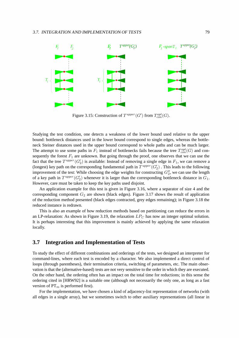
3.7. INTEGRATION AND IMPLEMENTATION OF TESTS 79
F1
Ti
F1
1
T 2upper(G’)
1
T (G’)21F i
upper-spanT
F1 F2
Ti
Figure 3.15: Construction of T upper (G′) from T optcon(G).
Studying the test condition, one detects a weakness of the lower bound used relative to the upperbound: bottleneck distances used in the lower bound correspond to single edges, whereas the bottle-neck Steiner distances used in the upper bound correspond to whole paths and can be much larger.The attempt to use some paths in F1 instead of bottlenecks fails because the tree T opt
con(G) and con-sequently the forest F1 are unknown. But going through the proof, one observes that we can use thefact that the tree T upper (G′
2) is available: Instead of removing a single edge in F1, we can remove a(longest) key path on the corresponding fundamental path in T upper (G′
2) . This leads to the followingimprovement of the test: While choosing the edge weights for constructing G ′′
2 , we can use the lengthof a key path in T upper (G′
2) whenever it is larger than the corresponding bottleneck distance in G1.However, care must be taken to keep the key paths used disjoint.
An application example for this test is given in Figure 3.16, where a separator of size 4 and thecorresponding component G2 are shown (black edges). Figure 3.17 shows the result of applicationof the reduction method presented (black edges contracted, grey edges remaining); in Figure 3.18 thereduced instance is redrawn.
This is also an example of how reduction methods based on partitioning can reduce the errors inan LP-relaxation: As shown in Figure 3.19, the relaxation LPC has now an integer optimal solution.It is perhaps interesting that this improvement is mainly achieved by applying the same relaxationlocally.
3.7 Integration and Implementation of Tests
To study the effect of different combinations and orderings of the tests, we designed an interpreter forcommand-lines, where each test is encoded by a character. We also implemented a direct control ofloops (through parentheses), their termination criteria, switching of parameters, etc. The main obser-vation is that the (alternative-based) tests are not very sensitive to the order in which they are executed.On the other hand, the ordering often has an impact on the total time for reductions; in this sense theordering cited in [HRW92] is a suitable one (although not necessarily the only one, as long as a fastversion of PTm is performed first).
For the implementation, we have chosen a kind of adjacency-list representation of networks (withall edges in a single array), but we sometimes switch to other auxiliary representations (all linear in

80 CHAPTER 2. REDUCTION TECHNIQUES
Figure 3.16: |S| = 4.
Figure 3.17: (|V | = 121, |E| = 200, |R| = 41).

3.7. INTEGRATION AND IMPLEMENTATION OF TESTS 81
Figure 3.18: (|V | = 121, |E| = 200, |R| = 41).
Figure 3.19: v(LPC) = 6393.

82 CHAPTER 2. REDUCTION TECHNIQUES
the number of edges) for certain operations. For each test, we perform all actions in a single pass (anddo not, for example, delete an edge and start the test from scratch). The details of the realization of thevarious actions are very technical and are omitted here; we merely mention that all actions followingeach test can be realized in a time dominated by the worst-case time O(m + n log n) of the fast tests.
With the additional requirement that in each loop of the selected tests a constant proportion (say5%) of vertices and edges must be eliminated and that instances of trivially small size are solveddirectly (by enumeration), one gets the same asymptotic time bound for the whole reduction processas for the first iteration (O(m + n log n), if one confines oneself to the fast tests).
Another technical aspect is the efficient reconstruction of a solution for the original instance outof a solution for the reduced instance (which often consists of a single terminal). Saving appropriateinformation during the reduction process, this can be done in time O(m). We always perform such atransformation after each run of the program, checking the feasibility and value of the solution in theoriginal instance.
3.8 Some Experimental Results
In this section, we present some summarized results of the reduction package on instance groups ofSteinLib (see Section 1.2 for a description of the problem instances). To give some impression of theeffect of the different approaches, we present results for different subsets of the reduction techniques:
O(m + n log n): In these runs, we have only included the fast versions of the reduction tests PTm,Triangle, NTDk, NV, SL, PS, VR, and LDA, which all can be implemented with a worst-caserunning time of O(m + n log n). For computing an upper bound, we used a fast path heuristicwith the same running time, which will be described in Section 4.2.
+ DUAL-ASCENT: These runs additionally use the DUAL-ASCENT algorithm, for generating alower bound, the calculation of an auxiliary graph for ASCEND-AND-PRUNE (see Sec-tion 4.4), and for bound-based reductions.
+ Extended Reduction Techniques: In this column, the extended reduction tests are also used. Notethat using extended reductions, there is an obvious tradeoff between reduction results and run-ning time, which can be configured by increasing or decreasing the parameter for the maximumbacktracking depth. A more detailed study of the results using extended reduction techniques isgiven in [PV01b].
+ Partitioning: Here, we additionally use the partitioning based reductions, presented in Section 3.6.As they require an exact solution of small subinstances, we also had to include the RG-testand branching, but only for the solution of the subinstances. Results including the RG-test arepresented in the context of the exact algorithm, in Section 5.4.
We know of only a few other works where the reported reduction results reach a quality that is atleast comparable to ours. One is the PhD thesis of Cees Duin [Dui93] who developed together withTon Volgenant several of the most important classical tests. He modified these tests so that they areapplicable at least to medium sized instances. Our results on these instances are similar, but in generalwe have better results: On the D-instances of SteinLib our fastest reductions already leave less than2% of the edges, while his leave 24%. (Duin did not give results on larger benchmark instances.)The best other results on these instances that were published in a journal are from Koch and Martin[KM98]. For the D-instances they achieve reduction to 38% of the edges of the original network.

3.8. SOME EXPERIMENTAL RESULTS 83
For VLSI instances, Uchoa, Poggi de Aragao, and Ribeiro [UdAR02] presented the best otherresults: With their reduction techniques only 6.2% of the edges remain, and the reductions took 367seconds on a Sun Ultra Sparc with 167 MHz. With our reductions, on the average only 0.05% of theedges remain after 4 seconds on a Sparc-III CPU with 900 MHz. A more detailed comparison of thetwo reduction packages is given in [PV01b, PV02a].
instance O(m + n log n) + DUAL-ASCENT + Extended Red. + Partitioninggroup time remaining time remaining time remaining time remaining
in sec. edges in % in sec. edges in % in sec. edges in % in sec. edges in %1R 0.08 57.41 0.12 45.60 0.32 0.00 0.20 0.002R 0.19 69.99 0.22 64.03 23.46 6.95 20.64 6.24D 0.08 1.46 0.07 0.52 0.64 0.35 0.31 0.14E 0.30 3.03 0.27 0.93 4.27 0.55 3.65 0.50ES10000FST 9.42 62.35 92.68 62.39 874.23 46.05 1048.04 17.41ES1000FST 0.58 62.67 0.80 62.79 4.82 46.83 9.63 20.32I080 0.02 43.62 0.02 26.77 0.06 20.63 0.09 15.95I160 0.05 63.98 0.06 33.61 0.31 28.77 0.43 25.60I320 0.19 71.82 0.31 47.51 2.48 40.07 3.42 35.72I640 0.96 79.88 1.89 53.17 15.32 45.12 25.33 43.29LIN 2.31 31.84 1.72 27.12 207.55 9.29 194.75 6.08MC 0.03 9.68 0.03 7.05 0.10 6.34 0.17 6.34PUC 0.34 99.33 0.89 99.33 7.67 99.31 12.77 99.31SP 0.17 37.50 1.39 37.50 5.75 37.50 7.81 37.50TSPFST 0.24 30.71 0.80 29.93 7.53 20.37 15.48 7.84VLSI 0.36 15.70 0.64 10.78 11.00 0.60 4.37 0.05WRP3 0.15 92.68 0.24 91.41 42.24 58.01 44.26 52.28WRP4 0.09 96.16 0.20 87.65 14.61 57.63 12.46 44.15X 0.34 0.39 0.31 0.00 0.28 0.00 0.32 0.00
Table 3.1: Some experimental results for reductions.
Chapter 4
Fast Computation of Short Steiner Trees
84
4.1. INTRODUCTION 85
4.1 Introduction
In this chapter, we focus on methods for computing upper bounds, in particular computing short (butnot necessary optimal) Steiner trees in short running times.
The number of papers on this topic is enormous, there are many heuristics and every popularmeta-heuristic has been tried (typically in many variants). A very comprehensive overview of articlespublished before 1992 can be found in [HRW92]. But the best results have been published after that(or have not yet even been published in a journal). In [PV97] we gave a comprehensive overview of themost important publications before 1997. Important recent developments can be found in [RUW02,PW02].
We have developed a variety of heuristics for obtaining upper bounds. Especially in the context ofexact algorithms very sharp upper bounds are highly desired. So, our main concern was achieving verystrong bounds, reaching the optimum as often as possible. On the other hand, the goal of obtainingshort total empirical running times prohibited us from using heuristics that achieve good solutionvalues only after long runs. In the following, we describe some of the methods we used in our attemptto achieve both goals simultaneously.
4.2 Path Heuristics
The repetitive shortest paths heuristic (SPH) is one of the empirically most successful classical heuris-tics for the Steiner problem in networks [TM80, HRW92, WS92, Voß92, PV01c, PW02]. The basicidea is to build a Steiner tree similar to Prim’s algorithm for the minimum spanning tree problem:Start with a subtree that initially consists of one vertex. In each step, connect the current subtreewith a shortest path to the next terminal. Repeat this until all terminals are connected. A final prun-ing step computes a minimum spanning tree of the vertices of the heuristic tree and removes non-terminals that have degree one in this tree. The worst-case running time for such a tree constructionis O(r(m + n log n)). To improve the quality of the solution, one usually repeats this process withdifferent start vertices (repetitive SPH).
For the computation of shortest paths in each iteration the algorithm of Dijkstra is used, whichuses tentative distances πi for every vertex vi ∈ V . A tentative distance πi represents an upper boundto the distance between the current subtree and vi. In [PW02] Poggi de Aragao and Werneck made asimple, but very effective observation: One does not have to reset tentative distances when a terminalis connected to the current subtree. The reason for this is that the old tentative distances are still validupper bounds for the distances from the extended subtree. All one has to do is reinsert every vertexvi into the priority queue of Dijkstra’s algorithm (with πi = 0) as soon as it becomes part of thecurrent subtree. Although the empirical running time is improved drastically, it is unsatisfying thatthe worst-case running time is still O(r(m + n log n)). Furthermore, as SPH is usually used in therepetitive variant, one can observe that very similar information is computed over and over withouttaking advantage of the previous computations.
Studying the repetitive shortest paths heuristic one observes that the actions can be divided intotwo phases (see [Dui93, DV97]): In the first phase, one can compute shortest paths from each terminalto all vertices; this can be done in time O(r(m+n log n)). Using the information from the first phase,each run of the SPH in the second phase (constructing a Steiner tree by successively connecting thecurrent tree (a single vertex at the beginning) to the closest terminal not in the tree by a shortest path)can easily be realized in time O(rn).
In [PV97, PV01c], we presented an efficient implementation of this approach and also a version

86 CHAPTER 4. FAST COMPUTATION OF SHORT STEINER TREES
with a worst-case running time of O(m + n log n). We will describe these heuristics in the next twosections. Note that we use these variants only as components of our other algorithms, not as stand-alone heuristics.
4.2.1 Faster Preprocessing for the Repetitive Shortest Path Heuristic
Our concern here is achieving empirical acceleration of the two-phase version of repetitive SPH.Regarding the first phase, we observe that the shortest paths need not be always computed completely:
Lemma 38 Let P be a shortest path between a terminal z and a vertex v, such that there is a vertex v ′
on P with z′ := base(v′) 6= z and d(z, z′) ≤ d(z, v). If v, but not z, belongs to the current tree T inthe second phase, there exists at least one other path connecting T to a terminal not in T which is notlonger than P . So, when computing shortest paths from z, we need consider neither v nor any vertexthat would become a successor of v in the shortest paths tree.
Proof: There are two cases:I) z′ ∈ T : Since d(z, z′) ≤ d(z, v), we can choose the path between z ′ and z.II) z′ /∈ T : Since d(z′, v) ≤ d(z′, v′) + d(v′, v) ≤ d(z, v′) + d(v′, v) = d(z, v), we can choose thepath between v and z′. 2
As a consequence, one can stop computing the shortest paths tree from a terminal z in the first phase assoon as the Voronoi region of z and the neighboring terminals (as defined in 1.3) have been spanned,because the shortest path between z and every vertex v visited afterwards contains a vertex v ′ ∈ N(z′)with z′ a neighbor of z and d(z, z ′) ≤ d(z, v), since z′ has already been spanned by the shortestpaths tree. Furthermore, no shortest path via an intermediary terminal needs to be considered. Theseobservations often lead to a considerable reduction in the empirical times, especially if the graph hasmany terminals and is not dense (the latter is almost always the case after reductions). Note that forgraphs with few terminals, repetitive SPH is fast anyway.
For building the Steiner trees in the second phase, we prefer a realization that uses the conceptof neighborhoods: Using the information from the first phase, we manage for each vertex v a list ofneighboring terminals, sorted by (increasing) distances to v. A priority queue manages candidatesfor expansion of the tree, using the distance to the nearest terminal not in the tree as the key forinsertion. Each time a vertex v is extracted from the queue, two cases can arise: Either the terminalcorresponding to the key is not yet in the tree, in which case the tree is expanded by the correspondingshortest path (and the queue is updated); or it is already in the tree, in which case the neighbor listof v is scanned further until either a terminal not in the tree is visited (which delivers the key forreinsertion of v into the queue) or the end of the list is reached (meaning that v can be ignored).Although the worst-case time of this implementation (O(rn log n)) is slightly worse than O(rn) ofthe straightforward implementations, it is usually much faster, and the worst-case time is dominatedby the first phase anyway.
4.2.2 A Path Heuristic with Good Worst Case Running Time
In situations where the worst-case time is the primary concern, we used a strengthening of the ideasabove to design a heuristic with time O(m + n log n). Motivated by the fact that the vicinity of eachterminal relevant for SPH often gets smaller with a growing number of terminals, one can simply forcethe first phase not to perform more than O(m+n log n) operations. But then it is no longer guaranteedthat the relevant neighborhood of each terminal is captured. To remedy this defect, we simultaneouslyuse the graph G′ of Mehlhorn’s fast implementation of T ′
D(R) [HRW92, Meh88], which we also

4.2. PATH HEURISTICS 87
compute in the first phase, see Section 1.3. In addition to the priority queue described above, a secondpriority queue, offering expansion of the current tree through edges of G′, is managed in the secondphase. For each expansion, the better offer is accepted and both queues are updated appropriately.
The information gained in the first phase can be used more economically if not only one, buta (constant) number of Steiner trees are computed in the second phase, using different terminals orvertices as starting points.
This heuristic can be implemented with time O(m + n log n) and guarantees a performance ratioof 2.
4.2.3 Some Experimental Results Of Path Heuristics
Although the path heuristics mentioned before were designed only to be used as a component ofother algorithms (especially in combination with reductions), they yield reasonable results even ontheir own. In Table 4.1, we give average running time and average gap from the optimal solution forinstances from SteinLib (see Section 1.2 for a description of the instance groups). The four algorithmscompared are the following:
one-phase SPH: One iteration of the simple shortest path heuristic, using the improvement of[PW02].
one-phase R-SPH: Repetitive variant of the above: Start from up to 100 different starting points(terminals are preferred as starting points).
two-phase R-SPH: Repetitive shortest path heuristic (up to 100 different starting points, terminalsare preferred), using the restricted preprocessing of distances and T ′
D(R) to achieve a worst-case running time of O(m + n log n).
T ′D(R): The distance network heuristic, for comparison with the two phase R-SPH.
All variants use the final minimum spanning tree pruning step, described above in the beginning ofSection 4.2.
One observes that due to the improvement of [PW02], the one phase SPH variant is very fast, butthe quality of the results is relatively weak. For this reason, the repetitive variant is usually used. Here,we see that using the fast two-phase variant can sometimes improve the running time. Furthermore,we can give an O(m + n log n) running time guarantee. The solutions quality produced by this two-phase variant is often the same as for the one-phase variant. This is due to the fact that in many casesthe computation is focussed very effectively by the application of Lemma 38, and in spite of the rigidrunning time guarantee, all necessary distances can be computed in the first phase. In these cases, dif-ferences in the quality of the solutions of the one-phase and the two-phase variant reflect only differentdecisions in situations when ties of paths of equal length are broken. A different situation happens forexample for the WRP3 and WRP4 instances, where many vertices are similarly close to many termi-nals. In the one-phase variant this leads to comparably high running times, as distance values have tobe rechecked again and again. In the two-phase O(m + n log n) variant, many computations in thefirst phase have to be aborted. As a consequence, for many paths, a precomputed shortest path is notavailable and one has two use paths from T ′
D(R) and the solution quality deteriorates.As a comparison we included the minimum spanning tree in the distance network T ′
D(R). Hereone sees that quality of the solutions is drastically improved with the two-phase variant, although thesame asymptotic running time guarantee can be given.
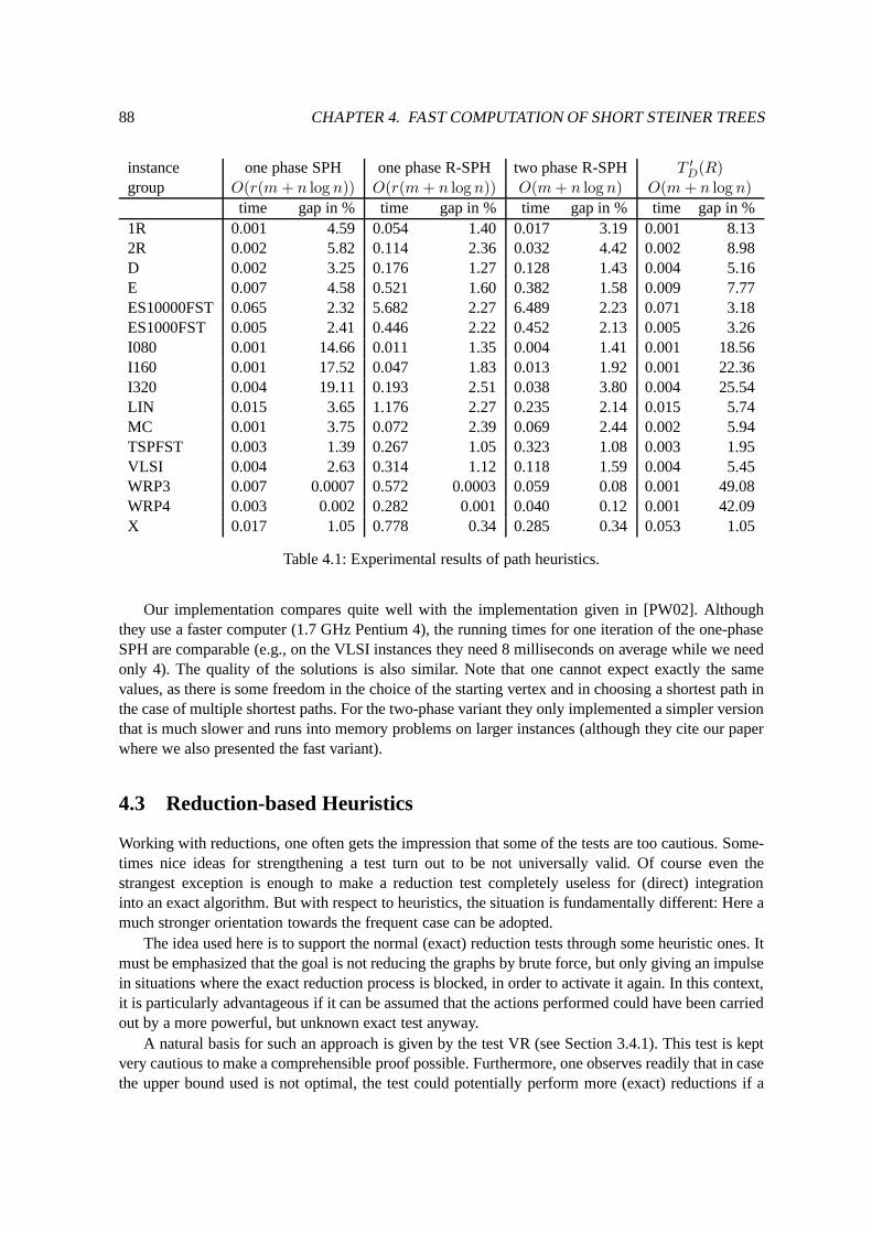
88 CHAPTER 4. FAST COMPUTATION OF SHORT STEINER TREES
instance one phase SPH one phase R-SPH two phase R-SPH T ′D(R)
group O(r(m + n log n)) O(r(m + n log n)) O(m + n log n) O(m + n log n)
time gap in % time gap in % time gap in % time gap in %1R 0.001 4.59 0.054 1.40 0.017 3.19 0.001 8.132R 0.002 5.82 0.114 2.36 0.032 4.42 0.002 8.98D 0.002 3.25 0.176 1.27 0.128 1.43 0.004 5.16E 0.007 4.58 0.521 1.60 0.382 1.58 0.009 7.77ES10000FST 0.065 2.32 5.682 2.27 6.489 2.23 0.071 3.18ES1000FST 0.005 2.41 0.446 2.22 0.452 2.13 0.005 3.26I080 0.001 14.66 0.011 1.35 0.004 1.41 0.001 18.56I160 0.001 17.52 0.047 1.83 0.013 1.92 0.001 22.36I320 0.004 19.11 0.193 2.51 0.038 3.80 0.004 25.54LIN 0.015 3.65 1.176 2.27 0.235 2.14 0.015 5.74MC 0.001 3.75 0.072 2.39 0.069 2.44 0.002 5.94TSPFST 0.003 1.39 0.267 1.05 0.323 1.08 0.003 1.95VLSI 0.004 2.63 0.314 1.12 0.118 1.59 0.004 5.45WRP3 0.007 0.0007 0.572 0.0003 0.059 0.08 0.001 49.08WRP4 0.003 0.002 0.282 0.001 0.040 0.12 0.001 42.09X 0.017 1.05 0.778 0.34 0.285 0.34 0.053 1.05
Table 4.1: Experimental results of path heuristics.
Our implementation compares quite well with the implementation given in [PW02]. Althoughthey use a faster computer (1.7 GHz Pentium 4), the running times for one iteration of the one-phaseSPH are comparable (e.g., on the VLSI instances they need 8 milliseconds on average while we needonly 4). The quality of the solutions is also similar. Note that one cannot expect exactly the samevalues, as there is some freedom in the choice of the starting vertex and in choosing a shortest path inthe case of multiple shortest paths. For the two-phase variant they only implemented a simpler versionthat is much slower and runs into memory problems on larger instances (although they cite our paperwhere we also presented the fast variant).
4.3 Reduction-based Heuristics
Working with reductions, one often gets the impression that some of the tests are too cautious. Some-times nice ideas for strengthening a test turn out to be not universally valid. Of course even thestrangest exception is enough to make a reduction test completely useless for (direct) integrationinto an exact algorithm. But with respect to heuristics, the situation is fundamentally different: Here amuch stronger orientation towards the frequent case can be adopted.
The idea used here is to support the normal (exact) reduction tests through some heuristic ones. Itmust be emphasized that the goal is not reducing the graphs by brute force, but only giving an impulsein situations where the exact reduction process is blocked, in order to activate it again. In this context,it is particularly advantageous if it can be assumed that the actions performed could have been carriedout by a more powerful, but unknown exact test anyway.
A natural basis for such an approach is given by the test VR (see Section 3.4.1). This test is keptvery cautious to make a comprehensible proof possible. Furthermore, one observes readily that in casethe upper bound used is not optimal, the test could potentially perform more (exact) reductions if a
4.4. RELAXATIONS AND UPPER BOUNDS 89
better upper bound was available. The idea is now to perform the usual actions of this test withoutan upper bound each time the other tests are blocked. At each application, a certain proportion ofvertices is eliminated (directly or after replacing of incident edges) according to the same criteria asin the exact version of the test (sum of distances to the next two or three terminals). Motivated bythe fact that for a large ratio r/n the alternative-based reductions are very successful anyway and thetest VR is usually effective only for small r/n, the proportion of the vertices being eliminated is afunction of n and r, getting smaller with growing r/n. With the additional postulation that duringeach application of the tests a constant percentage (say 5%) of vertices and edges is eliminated, theasymptotic time for all iterations together is the same as for the first one, namely O(m + n log n). Tomake sure that the instance is not made infeasible by the heuristic reductions, we further forbid directelimination of vertices in the current tree T ′
D(R). The computation of T ′D(R) also yields as a side
effect a guaranteed performance ratio of 2. We call this whole procedure PRUNE.The idea of not eliminating the nodes of a Steiner tree can be further utilized by using a (good)
heuristic solution instead of T ′D(R) for guiding the heuristic reductions. We use the implementation
of repetitive SPH described in Section 4.2 (with a constant upper bound for the number of repetitions)for this purpose, but any other good solution would do, too. On the other hand, we make the actionsof the heuristic reductions somewhat bolder, eliminating vertices only directly (without replacing ofincident edges). Note also that even Steiner nodes of the guiding heuristic solution may be eliminated,but only by the exact tests; these tests are guaranteed not to deteriorate the optimum. We call thisvariant of the PRUNE heuristic GUIDED-PRUNE.
4.4 Relaxations and Upper Bounds
Computing lower bounds is not the only motivation for dealing with relaxations; the informationobtained can also be used (among other things) to obtain upper bounds.
Consider the (directed) cut formulation PC of the Steiner problem: Given an optimal solution xof its linear relaxation LPC , the complementary slackness conditions state that each edge [vi, vj ] withxij > 0 has zero reduced cost. Assuming that there is some similarity between some optimal solutionsof the integer program PC and its linear relaxation LPC , it is well motivated to search an (optimal)solution in a subgraph containing the edges with reduced cost zero.
The algorithm DUAL-ASCENT, attempting to construct an optimal solution for DLPC , adjuststhe reduced costs favorably. So it is very natural to search for a solution in the set of edges whosereduced costs are set to zero by this algorithm, an idea already used in [Won84, Voß92]. The auxiliarygraph to be searched for a good solution need not contain all these edges; we have experimented withseveral schemes and gained the best overall results with a subgraph containing the (undirected edgescorresponding to) edges on zero-cost ways (with respect to reduced costs) from the root to anotherterminal, although other variants are not inappropriate either.
Having chosen such an auxiliary graph, the key question is how to obtain an (optimal) solutionfor the corresponding instance. The structure of such instances is very suitable for the applicationof our PRUNE heuristics; in particular, there are often long chains of vertices that are replaced bylong edges through the NTD2 test, making other alternative-based reductions very effective; and theheuristic reductions do the rest of the job. We call the whole procedure of doing fast reductions,calling DUAL-ASCENT, determining a subgraph and performing a PRUNE heuristic in the subgraphASCEND-AND-PRUNE.
Since we are working in a subgraph of G, the time bounds for the PRUNE heuristics (which aredominated by the worst case time of DUAL-ASCENT) are guaranteed in any case. Empirically, since
90 CHAPTER 4. FAST COMPUTATION OF SHORT STEINER TREES
the PRUNE heuristics run extremely fast on the auxiliary graphs, this kind of computation of upperbounds should be performed after each call to DUAL-ASCENT.
Although the experimental solution quality of this heuristic is impressive, it still sometimes missesthe optimum. We found out that in almost all such cases the reason is simply that the auxiliary graphdoes not contain an optimal solution (and not that the PRUNE heuristics do not find it). This observa-tion suggests a supplementation of this heuristic: The Steiner tree found in the subgraph can be usedas the guiding solution for a call to GUIDED-PRUNE in the original graph. In the cases mentioned,this approach often improves the solution value, frequently leading to the optimum.
By applying the idea of the PRUNE heuristics directly to the original graph, one can do withoutthe auxiliary graphs altogether. Let lower and c be the lower bound and the reduced cost vectorprovided by DUAL-ASCENT and x an optimal solution of PC with value optimum . The inequalityc · x ≤ optimum − lower (see Lemma 29) strongly suggests that normally there cannot be manyedges with large reduced costs in an optimal solution. This motivates another heuristic, SLACK-PRUNE, that basically follows the same scheme as GUIDED-PRUNE, but uses the criterion of thetest DA for eliminating vertices. The guiding solution is computed by a call of PRUNE in the auxiliarygraph described above, since the necessary information is available after performing DUAL-ASCENTanyway. The running time is dominated by the worst-case time of DUAL-ASCENT. Using the samearguments as in the case of PRUNE, one gets the time bound O(m ·minm,nr). But in combinationwith reductions, the empirical times are much smaller than the above term suggests.
As in DUAL-ASCENT, dual feasible solutions and corresponding reduced costs for LPC are cal-culated during the row generating algorithm (Section 2.9.2). This information can be used to generateauxiliary graphs similar to those in ASCEND-AND-PRUNE. But in this case there are not necessarilypaths with reduced cost zero from the root to all terminals. The auxiliary graph in this context containsall vertices with the property that there is a path from the root over this vertex to another terminal notlonger (with respect to reduced costs) than the longest shortest path from the root to another terminal.This auxiliary graph can be used as in ASCEND-AND-PRUNE.
A classical method for utilizing the information provided by linear relaxations is to use an ordinaryheuristic in the original network with modified edge costs c′ij = cij(1 − xij) (where x is the primalsolution of the current linear program). But this is not generally a good idea, because the structureof the primal solutions does not provide a good guide for a primal heuristic until the most advancedstages of the row generating algorithm.
These latter approaches only work in combination with explicit solution of linear programs andare therefore not suitable for fast, stand alone heuristics. But as a complement to the row generatingstrategy, they are frequently effective, especially in the advanced stages of the algorithm.
4.5 Combination of Steiner Trees
During the reduction process and especially while solving instances exactly, one usually gets severaldistinct heuristic solutions. In general, it is not the best idea to simply keep the best solution and forgetthe others. It is possible that solutions with a worse value are better locally, and one can try to keepthe best part of each solution.
We have developed several techniques for realizing the idea above. One simple and effective wayis to consider the graph consisting of the union of the edge sets of two (or more) Steiner trees. Inthis graph, one can call a (powerful) heuristic again or even try an exact solution. Such graphs havefrequently several (nontrivial) biconnected components, which makes the (exact) solution consider-ably faster. Using such schemes, we frequently get improvements in solution values (in case they

4.6. EXPERIMENTAL RESULTS AND EVALUATION 91
were not optimal anyway). Since the instances generated through such combinations (in the followingcalled combination-instances) are almost always solved to optimality through (fast) reductions, theseimprovements are gained at no significant extra cost.
For the results reported in this section, we simply call a PRUNE heuristic in such combination-instances; in particular, in the context of the heuristic SLACK-PRUNE we call the same heuristic(only without combinations) again in each combination-instance.
4.6 Experimental Results and Evaluation
In this section, we present some experimental results for reductions-based heuristics on instances from[SteinLib] (see Section 1.2 for a description of the instance groups). All of them are heuristics with aworst-case time describable by a polynomial of low order, as explained in the previous sections. Othergood heuristics in the literature can be found in [Dui93, DV97, Esb95, Ver96, RUW02].
For comparison, we include the results of Ribeiro, Uchoa, and Werneck [RUW02], which are thebest other results we are aware of. They use a combination of several techniques: A greedy random-ized adaptive search procedure (GRASP), a weight perturbation strategy (which uses the knowledgeof which edges are used frequently in many solutions), a local search procedure, a heuristic for thecombination of good solutions, and many reduction techniques. Unfortunately, they include a prepro-cessing for the D, E, and VLSI-instances in their runs, but did not include the preprocessing time inthe reported running times as we did. They report results only for those instances that could not besolved with their preprocessing routine, but we rescaled the values (assuming that instances solved bythe preprocessing produced an optimal solution in zero time), so that at least the values for the averagegaps are comparable. A stroke in the table means that no results were reported for these instances. Therunning times for [RUW02] where measured on a 300 MHz AMD and a Pentium II 400 MHz.
instance PRUNE ASCEND-&-PRUNE SLACK-PRUNE [RUW02]group time gap in % time gap in % time gap in % time gap in %1R 0.13 1.36 0.07 1.03 0.22 0.00 — —2R 0.27 1.42 0.16 1.59 10.91 0.00 — —D 0.10 0.07 0.07 0.02 0.14 0.00 > 11 0.04E 0.39 0.31 0.25 0.13 1.64 0.00 > 86 0.05ES10000FST 7.56 1.11 30.88 0.67 2101.89 0.38 — —ES1000FST 0.57 1.01 0.38 0.53 18.57 0.19 — —I080 0.07 1.15 0.02 1.65 0.43 0.06 > 2 0.01I160 0.31 1.97 0.07 1.69 1.68 0.10 > 16 0.13I320 1.63 2.84 0.30 1.81 7.46 0.14 > 108 0.15LIN 1.51 1.44 1.09 0.76 153.99 0.04 — —MC 0.05 1.70 0.04 1.01 0.95 0.42 — —TSPFST 0.21 0.42 0.38 0.31 32.01 0.04 — —VLSI 0.33 0.39 0.40 0.35 7.17 0.004 > 830 0.01WRP3 0.15 0.0006 0.14 0.0003 17.79 0.00003 — —WRP4 0.10 0.07 0.10 0.0006 6.19 0.00006 — —X 0.44 0.17 0.29 0.00 0.23 0.00 — —
Table 4.2: Some experimental results on upper bound calculation.

92 CHAPTER 4. FAST COMPUTATION OF SHORT STEINER TREES
From Table 4.2, one can see that SLACK-PRUNE is clearly superior to the approach of Ribeiro,Uchoa, and Werneck. Even taking into account the different speed of the machines, our approachis faster in most cases. Remember also that in [RUW02] the preprocessing time was not recorded.Additionally, the quality of the solutions produced by SLACK-PRUNE is better, even on the largerincidence instances (I160, I320), which were constructed to be difficult for the known reduction tech-niques. Note that the percentage of pruned vertices is a simple parameter for the tradeoff betweenrunning time and solution quality, i.e., better solutions can be achieved simply by decreasing thisparameter at the cost of longer running times.
The two heuristics PRUNE and ASCEND-AND-PRUNE are very fast while producing fairly goodresults. Note that PRUNE, although it has the better running time guarantee of O(m+n log n), in manycases takes longer than ASCEND-AND-PRUNE. The reason is that the techniques used in ASCEND-AND-PRUNE, in particular DUAL-ASCENT, are on the one hand much faster than the worst-casetime bound suggests, and on the other hand reduce a problem instance much more efficiently.

Chapter 5
Solving to Optimality
93

94 CHAPTER 5. SOLVING TO OPTIMALITY
5.1 Introduction
In this chapter, we present our results concerning the computation of optimal Steiner trees.As with the upper bound calculations, the number of competitors is huge: For every classical
approach (enumeration algorithms, dynamic programming, branch-and-bound, branch-and-cut) thereare many published results and the presented algorithms are sometimes quite involved. Again, wepoint to [HRW92] for a survey and only mention the most important updates:
• Duin [Dui93] improved the preprocessing techniques and invented some heuristics that wereintegrated into a branch-and-bound algorithm, which was clearly the best at its time.
• Koch and Martin [KM98] used some of the improved preprocessing techniques and developeda very powerful and robust branch-and-cut algorithm.
• Uchoa et al. [UdAR02] contributed some new extended preprocessing techniques (which werefurther generalized in Section 3.5). Their branch-and-cut algorithm is currently, to the best ofour knowledge, the best exact algorithm produced by other authors.
In the next section, we describe a dynamic programming approach that is useful for solving certainsmall subgraphs. After that we will describe the integration of the previously mentioned methods forreductions and upper and lower bound into an exact algorithm.
5.2 A Dynamic Programming Approach for Subgraphs
In this section, we present a practical algorithm for solving the Steiner problem in graphs with asmall width-parameter (a formal definition of width is given in the next section). The running timeof the algorithm is linear in the number of vertices when the width is constant, thus it belongs to thecategory of algorithms exploiting the fixed-parameter (FP) tractability of NP-hard problems. But theapplicability of this algorithm is much broader in the context of our work. Due to the use of reductiontechniques based on partitioning (Section 3.6) we can already profit from small width in subgraphsof the given instance. These techniques are in turn applicable to a very wide range of instances of theSteiner problem in networks after applying extended reduction methods (Section 3.5) and instancesof geometric Steiner problems after FST-generation [PV03, WWZ00].
The width-concept here is closely related to pathwidth. (For an overview of subjects concerningpathwidth and the more general notion of treewidth see [Bod93].) There are already FP-polynomialalgorithms for the Steiner problem in graphs; specifically, in [KS90] a linear-time algorithm for graphswith bounded treewidth is described. But this algorithm is more complicated than the one we presenthere, and its running time grows faster with the (tree-) width (it is given in [KS90] as O(nf(d))with f(d) = Ω(d4d), where d is the treewidth of the graph); so it seems to be not as practical asour algorithm, and no experimental results are reported in [KS90]. In a different context (networkreliability), a similar approach using pathwidth is described in [PT01], which is practical for a rangeof pathwidths similar to the one considered here. We also adapted this approach to the Steiner problem,but the experimental results were not as good as with the our approach.
A theoretically more powerful concept is the branch-width decomposition. It was formalized byRobertson and Seymour [RS91] and applied successfully to the TSP [CS02] and to the Steiner problemby Cook et. al. [Coo02]. We will not describe this approach, because experimental results showed thatno gain can be expected from it: Cook was not able to solve many instances of the TSPFST groupfrom [SteinLib], while we were able to solve them using a combination of our reduction techniques,

5.2. A DYNAMIC PROGRAMMING APPROACH FOR SUBGRAPHS 95
in particular the partitioning-based reductions (Section 3.6), and the Dynamic Programming approachfor subgraph presented in this section.
5.2.1 Additional Definitions
A path-decomposition of a graph G = (V,E) is a sequence of subsets of vertices (X1, X2, . . . , Xr),such that
1.⋃
1≤i≤r Xi = V ,
2. ∀(v, w) ∈ E ∃i ∈ 1, . . . , r : v ∈ Xi ∧ w ∈ Xi,
3. ∀i, j, k ∈ 1, . . . , r : i ≤ j ≤ k ⇒ Xi ∩ Xk ⊆ Xj .
The pathwidth of a path-decomposition (X1, X2, . . . , Xr) is max|Xi| | 1 ≤ i ≤ r − 1. Thepathwidth of a graph G is the minimum pathwidth over all possible path-decompositions of G.
5.2.2 The Algorithm
The outline of the algorithm is as follows: We maintain a set of already visited vertices and a subset ofthem (the border) that are adjacent to some non-visited vertex. In each step, the set of visited verticesis extended by one non-visited vertex adjacent to the border. For all possible partitions in each border,we calculate (the cost of ) a forest of minimum cost that contains all visited terminals with the propertythat each tree in the forest spans just one of the partition sets. We are finished when all vertices havebeen visited.
The motivation behind this approach is as follows: For any optimal Steiner tree T , the subgraphof T when restricted to the visited vertices is a forest, which also defines a partition in the border. Theplan is to calculate these forests in a bottom-up manner, in each step using the values calculated in theprevious step. If the size of all borders can be bounded by a constant, the total time can be boundedby the number of steps times another constant.
For an arbitrary fixed ordering v1, . . . , vn of the vertices and any s ∈ 1, . . . , n, we defineVs := v1, . . . , vs and denote with Gs the subgraph of G with vertex set Vs. In the following, weassume an ordering of the vertices with the property that all Gs are connected. (For example, a depth-first-search traversal of G delivers such an ordering.)
We denote with Bs the border of Vs, i.e., Bs := vi ∈ Vs | ∃(vi, vj) ∈ E : vj ∈ V \ Vs. WithLs we denote the set of vertices that leave the border after step s, i.e., Ls := (Bs−1 ∪ vs) \Bs. Theinclusion of vs in this definition should cover the case that vs has no adjacent vertices in V \ Vs; thissimplifies some other definitions.
Consider a set Q, Bs ∩ R ⊆ Q ⊆ Bs, and a partitioning P = P1, . . . , Pt of Q into nonemptysubsets, i.e., ˙⋃
1≤i≤tPi = Q and ∅ 6∈ P . For a partition P and a set L ⊆ V we define P − L :=P ′
i | Pi ∈ P, P ′i = Pi \ L. Let F (s,P) be a forest of minimum cost in Gs containing all terminals
in Vs and consisting of t (vertex-disjoint) trees T1, . . . , Tt such that Ti spans Pi for all i ∈ 1, . . . , t.With c(s,P) we denote the cost of F (s,P).
Let V0 = B0 = ∅ and set c(0, ∅) = 0. The value c(s,P) can be calculated recursively using a casedistinction:

96 CHAPTER 5. SOLVING TO OPTIMALITY
I) vs ∈ Q:
c(s,P) = minc(s − 1,P ′) + C | P ′ = P1, . . . , Pr, j ∈ 0, . . . , r,P = (vs ∪
⋃
1≤l≤j
Pl ∪ Pj+1, . . . , Pr) − Ls,
∀ 1 ≤ l ≤ j : vl ∈ Pl,
C =∑
1≤l≤j
c(vl, vs),
II) vs 6∈ Q:c(s,P) = min c(s − 1,P ′) | P = P ′ − Ls.
The cost of an optimal Steiner tree in G is
min c(s,P) | R ⊆ Vs, |P| = 1.
Obviously the forests F (s,P) (and an optimal Steiner tree) can be calculated following the samepattern.
5.2.3 Dynamic Programming Implementation
By using the recursive formula above, the necessary values can be calculated in a bottom-up mannerby memorizing, for each step s, the values c(s,P). We assume c(s,P) = ∞ if no partition P iscalculated at step s. This leads to the following algorithm, written in pseudocode:
1 s = 0; r = 0; opt = ∞; “r : number of visited terminals”2 c(s, ∅) = 0;3 while s < n :4 s = s + 1; determine vs, Bs and Ls;5 if vs ∈ R : r = r + 1;6 forall P with c(s − 1,P) 6= ∞ :7 oldCost = c(s − 1,P);8 if vs 6∈ R and ∅ 6∈ P − Ls :9 c(s,P − Ls) = oldCost ;10 Pcandidates = Pi ∈ P | ∃vi ∈ Pi : (vi, vs) ∈ E;11 forall Pconnect ⊆ Pcandidates :12 connectionCost=
∑
Pi∈Pconnect minvi∈Pi,(vi,vs)∈E c(vi, vs);
13 Pstay = P\Pconnect ; Pnew = (vs ∪⋃
Pi∈Pconnect Pi ∪ Pstay) − Ls;14 if ∅ 6∈ Pnew and c(s,Pnew) > oldCost + connectionCost :15 c(s,Pnew) = oldCost + connectionCost;16 if r = |R| and |Pnew| = 1 : “feasible Steiner tree”17 opt = min(opt, c(s,Pnew));
5.2.4 Running Time
Let ps denote the number of partitions at step s. We have
ps =∑
R∩Bs⊆Q⊆Bs
|Q|∑
i=1
|Q|i
=∑
R∩Bs⊆Q⊆Bs
B(|Q|),
5.2. A DYNAMIC PROGRAMMING APPROACH FOR SUBGRAPHS 97
where B(b) is the b-th Bell number; so ps = O(2bsB(bs)) with bs := |Bs| . We only main-tain one global list of partitions, which is updated after each step, keeping for each valid parti-tion a solution of minimum cost. Because of the loop in line 11, this list can grow to at mostls := 2bsps = O(22bsB(bs)) partitions. Eliminating the duplicates can be done by sorting the list:Each partition can be represented as a (lexicographically) sorted string (of length at most 2bs) ofsorted substrings (of length at most bs) separated by some extra symbol. Using radix sort, all the in-dividual sortings of ls strings can be done in total time O(n + lsbs). Sorting the resulting list of lsstrings takes again O(n+ lsbs). We set aside for now a total extra time of O(|E|) for the operations onedges; and assume that an ordering of vertices is given (these points are explained below). The (restof the) operations in lines 12 − 17 can be carried out in time O(bs). This gives the total running timeO(
∑ns=1 bs2
2bsB(bS)). Note that this bound implicitly contains the extra amortized time O(|E|) bythe following observation: After a vertex is visited for the first time, it remains in the border as longas it has some non-visited adjacent vertex; so each edge is accounted for by its first-visited endpoint.
Now if we can guarantee an upper bound b for the size of all borders, we have an upper boundof O(nb22bB(b)) for the running time. Using the very rough upper bound (2b)b for B(b) we get therunning time: O(n2b log b+3b+log b). This means that the algorithm runs in linear time for constant band, for example, in time O(n2) for b = O(log n/ log log n).
For the actual implementation, some modifications are used. For example, avoiding duplicatepartitions is done using hashing techniques, which reduces the amount of necessary memory.
5.2.5 Ordering the Vertices
In Section 5.2.6 we will show that finding an ordering of vertices such that the maximum border sizeequals b is (up to some easy transformations) equivalent to finding a path-decomposition of pathwidthb. The problem of deciding whether the pathwidth of a given graph is at most b, and if so, findinga path-decomposition of width at most b is NP-hard for general b [ACP87], but for constant b, thisproblem can be solved in linear time [Bod96]. However, already for b > 4 the corresponding algorithmis no longer practical [R oh98], and it seems that no practical exact algorithm is known for more generalcases [Bod02]. Furthermore, we have a more specific scenario; for example we differentiate betweenterminals and nonterminals. So for the actual implementation we use a heuristic, which has producedquite satisfactory results for our applications. The heuristic chooses in each step a vertex vs adjacentto the border using a (ad hoc) priority function of the following parameters:
• size of resulting set Ls,
• number of visited vertices in the adjacency list of vs,
• is vs a terminal (1/0),
• number of edges connecting Vs and V \ Vs.
We select the starting vertex by trying a small number of terminals and performing a sweepthrough the graph without actually computing the partitions, but by estimating their number usinganother (ad hoc) function and selecting the one with the smallest overall value.
A straightforward implementation of this heuristic needs time O(n2) for all choices. This boundcould be improved using advanced data structures for priority queues and additional tricks, but theordering has not been the bottleneck in our applications; and theoretically a better (linear for constantb as in our applications) time bound for path-decomposition is available anyway.

98 CHAPTER 5. SOLVING TO OPTIMALITY
5.2.6 Relation to Pathwidth
In this section, we show that every path-decomposition with pathwidth k delivers a sequence of bor-ders B = (B1, . . . , Bs, . . . , Bn) such that max|Bs| | 1 ≤ s < n ≤ k and vice versa.
First, note that the 3rd condition in the definition of path-decomposition can be rewritten as fol-lows: There are functions start , end : |V | → 1, . . . , r with v ∈ Xj ⇔ start(v) ≤ j ≤ end(v).
We call a path-decomposition bijective if the mapping start is a bijection.
Lemma 39 Every path-decomposition X = (X1, . . . , Xr) can be transformed to a bijective path-decomposition (X ′
1, . . . , X′n) of no larger pathwidth.
Proof: We modify the sequence X as follows:As long as there is some i with start−1(i) = ∅, remove Xi from X; adapting the functions start
and end .As long as there are v 6= v′ with start(v) = i = start(v′), define Xj+1 = Xj for all j ≥ i andremove v′ from Xi; adapting the functions start and end .One easily observes that the final resulting sequence X ′ satisfies the properties for a path-decomposition, is bijective, and has no greater pathwidth. 2
We call a path-decomposition with functions start , end minimal if it holds:
end(v) ≥ i ⇒ start(v) = i ∨ ∃(v, w) ∈ E : start(w) ≥ i.
(Note that the other direction is satisfied for every path-decomposition.)
Lemma 40 Every (bijective) path-decomposition X can be transformed to a minimal (bijective) path-decomposition of no larger pathwidth.
Proof: For every v, set end(v) := maxstart (w) | (v, w) ∈ E ∨ v = w. Delete v from all Xi
with i > end(v). One easily observes that the resulting sequence satisfies the properties for a path-decomposition, has no greater pathwidth, is minimal, and remains bijective if the original decompo-sition was bijective. 2
Lemma 41 Let (X1, . . . , Xn) be a minimal, bijective path-decomposition of G with the functionsstart and end . Assume that the vertices are ordered according to their start values, i.e., start(v) =s ⇔ v ∈ Vs \ Vs−1. For each s ∈ 1, . . . , n it holds: Xs = vs ∪ Bs−1.
Proof:
v ∈ Xs ⇔ start(v) ≤ s ∧ end(v) ≥ s
⇔ (start(v) = s ∨ start(v) < s) ∧ (start (v) = s ∨ ∃(v, w) ∈ E : start(w) ≥ s)
⇔ start(v) = s ∨ (start(v) < s ∧ ∃(v, w) ∈ E : start(w) ≥ s)
⇔ v = vs ∨ (v ∈ Vs−1 ∧ ∃(v, w) ∈ E : w ∈ V \ Vs−1)
⇔ v = vs ∨ v ∈ Bs−1
2
It follows that every path-decomposition of G can be transformed to a path-decomposition X =(X1, . . . , Xn) of no larger pathwidth such that for an ordering of vertices according to the start
function of X it holds: Xs = vs ∪ Bs−1. On the other hand, it is easy to verify that each orderingof vertices and the corresponding sequence of borders (B1, . . . , Bn) deliver a (minimal, bijective)path-decomposition X by setting Xs = vs ∪ Bs−1. In each case, we have: max|Xs| | 1 ≤ s ≤n − 1 = max|Bs−1| | 1 ≤ s ≤ n.

5.3. PUTTING THE PIECES TOGETHER: THE EXACT ALGORITHM 99
5.3 Putting the Pieces Together: The Exact Algorithm
In this section we describe the synthesis of an exact algorithm from the components described in theprevious sections.
5.3.1 Interaction of the Components
A central feature of our exact algorithm is that the various components (reduction tests, lower boundsand upper bounds) do not act independently of each other, as described in detail in previous sections:
Reductions
Upper Bounds Lower Bounds
Figure 5.1: Interaction of the different components.
The bound-based reductions depend on upper and lower bounds; and the computation of upper andlower bounds profits from reductions, both in terms of running time and quality of results. The ideabehind reduction tests is also the central part of the reduction-based heuristics for computing upperbounds. Further we use the structure of heuristic solutions (corresponding to good upper bounds) toguide the computation of lower bounds; and the information gained during the computation of lowerbounds is used to guide the computation of upper bounds. All in all, there is a mutual dependencebetween the three major components: reductions, upper bounds, and lower bounds. This is not adrawback, but an advantage: The scenario is that performing (alternative-based) reductions acceleratesthe computation of upper and lower bounds and enhances their qualities; the information gained duringthe computation of bounds is used to reduce the instance further (using bound-based reductions), andthen the whole pattern repeats. We call this whole process the reduction process, beginning with fastreductions and switching to more and more powerful ones as the process advances. This strategy isnot only a major reason for the short solution times our algorithm very often achieves, but also enablesinstances to be solved that we could not solve in a reasonable time otherwise. Note especially that thevalue of the lower bound corresponding to a certain relaxation can be enhanced through reductions;this helps to solve instances that otherwise could not be solved (without branching) using the sametechniques for computing upper and lower bounds.
For the experimental results given in this chapter, we use the following components: For com-puting lower bounds, we use the relaxation LPC through the algorithm DUAL-ASCENT and, inadvanced stages, row generation with LPC′ (Section 2.9.2) or, if the proportion of terminals to allvertices is high, the Lagrangian relaxation LaPT0
(Section 2.9.1). To reduce the instances, we use alldescribed alternative-based techniques (Section 3.3). In addition, we use the bound-based techniquesDA (Section 3.4.2) and, in combination with row-generation, the test RG (Section 3.4.3). Further-more, we use the extended reduction techniques (Section 3.5) and the partitioning-based reductions(Section 3.6). For computing upper bounds we use our PRUNE heuristics (Sections 4.3, 4.4), includ-ing the combination of Steiner trees (Section 4.5). Before starting the time-consuming RG reduction

100 CHAPTER 5. SOLVING TO OPTIMALITY
test, we check with the heuristic mentioned in Section 5.2 whether we can solve the (sub-)instancewith the pathwidth approach.
As described above, the fast methods are applied first, with switching to more time-consumingones only if an instance has not already been solved to optimality. Apart from this general principle,the exact ordering of the components has usually not been critical.
5.3.2 Branch-and-Bound
The reduction process described in the previous subsection is an extremely powerful device, but itis not guaranteed to solve every instance of the problem. To get an exact algorithm, we integrate itinto a branch-and-bound framework. But one should not be misled by the name branch-and-bound:Branching is something we generally (and often successfully) try to avoid, it is only a safety net incase the reduction process is blocked. This also means that we invest a lot of work in each node ofthe branch-and-bound tree to keep the tree small, and do not try to gain speed by limiting the work ineach node.
We use binary, vertex-oriented forward branching [HRW92]. Both depth-first and best-first searchstrategies are available in our implementation, with depth-first as default. There are usually not manynodes in our branch-and-bound trees anyway; moreover, only the currently processed node needs tobe kept in the main memory.
As the branching variable, we choose the non-terminal with the largest degree in the best availableSteiner tree. The intuitive motivation for this choice is an intensification of the search in an area wherea good solution has been found (in case of inclusion) and a diversification of the search to otherareas (in case of exclusion). This strategy also supports the building of several blocks (biconnectedcomponents). It is known [HRW92] that in case several blocks exist, the problem can be solved bysolving the instances corresponding to each intermediate block separately, which generally reducesthe total running time substantially. Although it usually cannot be assumed that the original instanceis not biconnected, this often changes later during the reduction process and after branching. We usethis fact frequently in our algorithms: Whenever a more time-consuming part is to be performed, wecheck whether the graph is biconnected. If this is not the case, we solve the corresponding subinstancesseparately and transform the information gained back to information for the original instance. Hereone can use the following observation to identify the blocks that must be considered:
Lemma 42 Let T be a Steiner tree with all leaves being terminals in a network G. A block of G isintermediate if and only if it contains an edge of T .
Proof: For a block B to be intermediate, there must be two terminals zk and zl such that every pathbetween zk and zl contains an edge in B. Hence, every Steiner tree must contain an edge in B.Conversely, consider a Steiner tree T with all leaves being terminals that contains an edge in a blockB. So there are two terminals zk and zl such that at least one path between zk and zl contains an edgein B. If zk (or zl) is in B and it is not an articulation point, B is obviously intermediate. Otherwisethere must be two articulation points vi and vj of B such that a path between zk and vi and a pathbetween vj and zl contain no edge in B. Now suppose B is not intermediate. Then there is a pathbetween zk and zl that does not contain an edge in B. Hence, there is also a path between vi and vj
that has no edge in B, which contradicts the definition of B as a biconnected component. 2

5.4. SUMMARY ON EXPERIMENTAL RESULTS 101
5.4 Summary on Experimental Results
Here we report on what the components presented achieve together, acting as an “orchestra”. As statedin Section 1.2, results for different types of instances from the benchmark SteinLib are presented,including the instances of the OR-Library. Here we give only averages for some groups of instances.In the appendix, we report on the results for each instance separately.
We leave it mainly to the reader to compare the given running times to those of other exact al-gorithms in the literature (see for example [Bea89, BL98, CGR92, Dui93, KM98, Uch01]). As anorientation, we provide in Table 5.1 the average times (in seconds) for the exact solution of someinstances groups, which have frequently been used by other authors. It is true that we used the fastestmachine (it is approximately half as fast as the PC we used in Section 5.4.1); however improvedmachine speed explaines our improved times only to a small extend.
instance- [Bea89] [BL98] [CGR92] [Dui93] [KM98] [Uch01]∗ heregroup Cray X-MP SG Indigo VAX 8700 i486 Sun Sparc 20 UltraSparc II Sunfire
D 556 3545 14260 176 117 > 4 0.2E — — — — 4415 > 181 1.7
TAQ† — — — — 197 4 0.08TAQ — — — — — 162 1.1
Table 5.1: Average running times of different exact algorithms.
We solved all instances that (to our knowledge) have been solved before. Furthermore, we solved32 instances from different instance classes from SteinLib (geometric (TSPFST), VLSI (LIN), wirerouting problems (WRP3), constructed difficult instances (I640, PUC, SP) that have not been solvedby other authors. See the appendix for details.
5.4.1 Experimental Results on Geometric Instances
As mentioned already in Sections 1.4.2 and 3.6.1 for geometric Steiner problems, an approach basedon full Steiner trees (FSTs) has been empirically successful [WWZ00]: In the first phase, the FSTgeneration phase, a set of FSTs is generated that is guaranteed to contain an SMT. In the secondphase, the FST concatenation phase, one chooses a subset of the generated FSTs whose concatenationyields an SMT. Empirically, the second phase was usually the bottleneck, where originally methodslike backtracking or dynamic programming have been used. A breakthrough occured when Warme[War98] used the fact that FST concatenation can be reduced to finding a minimum spanning tree ina hypergraph whose vertices are the terminals and whose (hyper-)edges correspond to the generatedFSTs. We use a different approach: By building the union of (the edge sets of) the FSTs generatedin the first phase, we get a normal graph and the FST-concatenation problem is reduced to solvingthe classical Steiner problem in this graph. Note that in this way the useful information about theindividual FSTs is lost. Still, our approach is much faster. In Table 5.2, we compare for the secondphase the running times of our program and of the program package GeoSteiner [WWZ01]. For moredetailed results on this, see [PV03, PV01d].
∗In [Uch01] only running times for 5 of the 40 D/E instances are reported, we estimated the averages by assuming thatall other instances were solved in zero time.
†Excluding instances not solved by [KM98].

102 CHAPTER 5. SOLVING TO OPTIMALITY
For both programs all computation was performed on a PC with an AMD Athlon XP 1800+ (1.53GHz) processor and 1 GB of main memory, using the operating system Linux 2.4.9. We used the gcc2.96 compiler and CPLEX 7.0 as LP-solver.
instance GeoSteiner our programgroup time (s) time (s)ES1000FST 150.6 10.3TSPFST‡ 261.8 3.0
Table 5.2: Comparison of GeoSteiner (2nd phase) and our program (average running time for exactsolution).
Additionally, we are able to solve some instances (fl1400, fl3795, fnl4461) that have not beensolved before. In Table 5.3, we show results for instances not solved by GeoSteiner in one day.
instance size optimum our program|R| |V | |E| time (s)
es10000 10000 27019 39407 716174280 758fl1400 1400 2694 4546 17980523 118fl3795 3795 4859 6539 25529856 139fnl4461 4461 17127 27352 182361 6148pcb3038 3038 5829 7552 131895 2.4pla7397 7397 8790 9815 22481625 0.1
Table 5.3: Instances not solved by GeoSteiner in one day.
5.5 Concluding Remarks
We have presented several algorithmic contributions for solving the Steiner problem in networks. Theexperimental results strongly recommend the chosen approach based on reductions and underline theutility of the techniques presented here. In particular, the reduction-based heuristics have proven tobe extremely strong and robust. Also, the running times of the exact algorithm are often surprisinglysmall; and for many instances, there is not much room left for improvements. But this is not alwaysthe case:
For some instances, fast reductions come to a halt at a time when the relaxations used are stillnot strong enough; this is for example the case for some of the MC- and I-instances, which wereinsightfully constructed to fool the currently available techniques. Here, the algorithm has gone intobranching to solve the instances exactly. Until new techniques are developed, instances of this typewith thousands of vertices will not be solvable in reasonable time. But the results for the other groupsof instances seem to indicate that such cases rarely arise naturally.
With respect to instances that were not artificially constructed, even instances with tens of thou-sands of vertices can usually be solved in reasonable time. Of course, very large instances are still achallenge. There are two main problems:
First, even though the running time and memory consumption for many components can be de-scribed by polynomials of low degree, they can grow to a critical value for very large instances. Es-pecially, the Θ(rn) memory consumption of the DUAL-ASCENT procedure, which is used relatively
‡Excluding instances not solved by GeoSteiner.

5.5. CONCLUDING REMARKS 103
early in the reduction process, can be a limiting factor. To overcome this problem, the developmentof new fast reduction techniques could be a solution. If they combine low memory consumption, fast(empirical) execution times and relevant reduction results, they could prepare the ground for currentlyavailable reduction techniques.
A second reason is even more decisive. As already discussed in Section 3.6.3, the LP-based ap-proaches rely on the quality of the Linear Programming relaxation used, but any LP-relaxation ofpolynomial size is bound to have some (integrality) gap in this context. In larger instances, such gapscan accumulate and become more and more relevant. In particular, the important bound-based reduc-tions lose their impact if the available bounds are too weak. There are several approaches to addressthis:
Branch-and-cut: Currently, we do not use the branch-and-cut approach to improve the quality of thelower bound calculation. The reason is that we found it more advantageous to use the calculatedlower bound to reinforce the reduction process, i.e., we use the lower bound and reduced costsfor bound-based reductions and then try all reduction tests on the reduced graph. This procedureis often sufficient to solve problem instances without branching. Even if branching is necessary,the whole reduction processes can try to make use of the vertex branching, which is not thecase in a branch-and-cut setting, because for many operations performed by reduction tests(e.g., replacement of a vertex by a clique over its neighbors, see Section 3.3.2) there are nomethods available to translate them profitably into the linear program maintained by the branch-and-cut algorithm. On the other hand, our approach has the disadvantage that the generatedconstraints will be discarded after the row generation test (RG) is finished and for the next RGtest, they have to be computed from scratch. For medium sized instances this disadvantage isnot important, as the row generation is not too time consuming. For larger instances where mostof the time is spent solving linear programs, a better integration of the reductions into a rowgeneration or branch-and-cut approach could be an improvement.
Using tighter relaxations: In Section 2.9.3, we showed how to use a tighter linear relaxation effi-ciently. Other, even tighter relaxations are available in the hierarchy of relaxations, presented inSection 2.8, but currently no technique is at hand to use them in such an efficient way that theycould be applied to larger problem instances.
Improving linear relaxations outside the template paradigm: We have already discussed two ad-vanced techniques, the local cuts approach and the graph expansion approach, in the concludingremarks on lower bounds, Section 2.11. A further development of these techniques could en-large the range of solvable instances.
For geometric instances, we have shown that a combination of full Steiner tree (FST) approach(see the results in the last section) that exploits the geometric properties of the problem and ouralgorithm for the Steiner problem in general networks is currently the most successful approach.However, it should be possible to improve on this, as a lot of useful information is discarded whenthe set of FSTs is converted into an instance for the network Steiner tree problem. Exploiting thisinformation in our approach, or integrating our reduction techniques into the FST approach could befruitful.
Another algorithmic challenge for Steiner tree algorithms is the development of algorithms forreliable computation [Meh02], i.e., algorithms that come with some kind of evidence that they pro-duce correct results. As a formal verification of the whole program is unlikely, certifying algorithmsas components would already be an advantage. Such algorithms return additional output (frequently
104 CHAPTER 5. SOLVING TO OPTIMALITY
called a witness) that enables a (fast) verification of the results. A weak version of a witness is men-tioned in Section 3.7: After all reductions are performed, the algorithm can transform a tree in thereduced instance into one for the unreduced instance, thus certifying that a tree with the same valueexists in the original instance. Of course, this says nothing about the optimality of this tree. Otherparadigms of reliable computation, namely “exact arithmetic” and “test and repair” have been men-tioned in the context of using linear programming packages for reductions in Section 3.4.3. We listsome of the major problems for certifying algorithms in the context of reduction techniques:
• A difficulty arises from a pattern that is frequently used in the efficient implementation of re-duction tests: First, in a preprocessing step, some data structures are set up (e.g., representing aSteiner tree produced by some heuristic, a minimum spanning tree T ′
D(R) in the distance net-work, approximations of distances and bottleneck Steiner distances, a lower bound and reducedcosts). Then, reduction tests use these data and modify the network. These modifications aredone in such a way that the precomputed information is still valid (e.g., the extension of thePTm-test to the case of equality in Section 3.3.1) or that invalid parts are marked such they donot cause harm (e.g., the neighbor lists used for tagging precomputations as invalid if an edgeis deleted in Section 3.5.5).
Even if it was possible to verify that the data structures were correct for the original network,it could be very difficult to verify that they are used correctly after the network is modified. Asimple example is the following: When the first edge is deleted by the PTm-test (Section 3.3.1),it is easy to verify that a path exists with Steiner distances not longer than the length of the edgeby following the parent pointers in the shortest path tree and the T ′
D(R) edges. For edges thatare deleted later, this is no longer possible directly, as edges on this path may have been deleted.
• For many certifying algorithms the running times for producing the witness and verification ofthe result is (at least asymptotically) dominated by the running time for the algorithm. For thepresented reduction tests with running time O(m + n log n) this is not an easy task. Note thatone of the major contributions of this work are the techniques for performing reduction testsso fast that they can be applied extensively. As a consequence, if a certifying reduction test ismuch slower than the original version, it cannot be applied in the same way as before.
In the example above, checking the edges of the alternative path can take time O(n), while thetest condition of the PTm test can be checked in nearly constant time.
Finally, it is an interesting open question whether the concepts presented in this work can beadapted to other combinatorial optimization problems. Promising candidates for such a recycling ofideas are the reduction-based heuristics (Section 4.3) and extended reduction techniques (Section 3.5)for problems where reduction techniques are already known, and partitioning as a reduction technique(Section 3.6) and graph expansion for improving lower bounds (sketched in Section 2.11) for generaloptimization problems in networks.
Appendix A
Experimental Results of the ProgramPackage
Here we report on what the components presented achieve together, acting as an “orchestra”. In Ta-bles A.2-A.11 we report on each instance of SteinLib, except for the instance groups I080, B, C, P,and ES10FST–ES500FST, which are too easy. Overall we report on 831 instances.
All results were produced by a single run of the same program with the same parameter values,with the exception of the instance groups I and PUC. These instances were constructed with theaim of being difficult for known techniques, thus currently many of them can only be solved usingmany branching nodes in a branch-and-bound framework. Therefore, we made the solution faster byomitting the time consuming row generation method (Section 2.9.2) in the reduction process. Notethat instances that arise naturally from some application can often be solved without branching byusing the sophisticated reduction techniques.
For each instance, we give the value of the optimal solution and the total time until the exactsolution of the instance (in seconds). We set a time limit of five hours on each run. Within this time, wehave solved most of the considered instances. Only 64 instances have not been solved within the timelimit. For these instances we give the upper and the lower bound after five hours (in italics). However,9 of these instances could be solved using stronger extended reductions (see Section 3.5), and 12 couldbe solved by longer runs. For them we give the time for the exact solution in Tables A.14 and A.15. Intotal, there are only 43 unsolved instances left. These instances are from the instance groups SP, PUC,and I640, which where constructed with the aim of being difficult for known techniques.
We solved all instances that (to our knowledge) have been solved before. Furthermore, we solved32 instances from different instance classes from SteinLib that have not been solved by other authors(see Table A.1).
In many cases our program performs several orders of magnitude faster than programs of otherauthors, see Section 5.4 for a short comparison with others’ results. It is acknowledged to be thestrongest program for solving general Steiner problem instances at the time being [CD01, SteinLib].
All results in this work were produced single-threaded on a Sunfire 15000 with 900 MHz SPARCIII+ CPUs, using the operating system SunOS 5.9. We always used the GNU g++ 2.95.3 compiler withthe -O4 flag. As it is a multi-processor machine with shared memory, it is slower than a single proces-sor system with the same processor. A comparison with the running times reported in Section 5.4.1shows that the machine is approximately half as fast as a PC with an AMD Athlon XP 1800+ (1.53GHz) processor.
105

106 APPENDIX A. EXPERIMENTAL RESULTS OF THE PROGRAM PACKAGE
Instance Group Table InstancesLIN A.5 lin31, lin32, lin33, lin34, lin35, lin36, lin37WRP A.4 wrp3-83TSPFST A.6 fl1400fst, fl3795fstPUC A.12 bipe2p, bipe2u, cc5-3p, cc5-3u, hc8p, hc8uSP A.13 w3c571I640 A.11 i640-211, i640-212, i640-213, i640-214, i640-215,
i640-321, i640-322, i640-323, i640-324, i640-325,i640-341, i640-342, i640-343, i640-344, i640-345
Table A.1: Instances solved by us and not solved by others.
Instance Size Opt Time|V | |E| |R|
d01 1000 1250 5 106 0.1d02 1000 1250 10 220 0.1d03 1000 1250 167 1565 0.1d04 1000 1250 250 1935 0.1d05 1000 1250 500 3250 0.1d06 1000 2000 5 67 0.3d07 1000 2000 10 103 0.3d08 1000 2000 167 1072 0.1d09 1000 2000 250 1448 0.1d10 1000 2000 500 2110 0.1d11 1000 5000 5 29 0.2d12 1000 5000 10 42 0.1d13 1000 5000 167 500 0.1d14 1000 5000 250 667 0.1d15 1000 5000 500 1116 0.1d16 1000 25000 5 13 0.2d17 1000 25000 10 23 0.2d18 1000 25000 167 223 0.7d19 1000 25000 250 310 0.5d20 1000 25000 500 537 0.1
Instance Size Opt Time|V | |E| |R|
e01 2500 3125 5 111 0.5e02 2500 3125 10 214 0.3e03 2500 3125 417 4013 0.1e04 2500 3125 625 5101 0.1e05 2500 3125 1250 8128 0.1e06 2500 5000 5 73 1.2e07 2500 5000 10 145 1.1e08 2500 5000 417 2640 0.2e09 2500 5000 625 3604 0.1e10 2500 5000 1250 5600 0.1e11 2500 12500 5 34 0.8e12 2500 12500 10 67 0.6e13 2500 12500 417 1280 1.3e14 2500 12500 625 1732 0.2e15 2500 12500 1250 2784 0.2e16 2500 62500 5 15 0.8e17 2500 62500 10 25 0.5e18 2500 62500 417 564 21.6e19 2500 62500 625 758 4.1e20 2500 62500 1250 1342 0.2
Table A.2: Results on the D and E-instances. Type: Sparse random with varying graph parameters,OR-Library.
Instance Size Opt Time|V | |E| |R|
1r111 625 2352 6 28000 0.21r112 625 2352 6 28000 0.11r113 625 2352 6 26000 0.11r121 625 2340 6 36000 0.11r122 625 2342 6 45000 0.71r123 625 2343 6 40000 0.31r131 625 2336 6 43000 0.41r132 625 2340 6 37000 0.11r133 625 2326 6 36000 0.11r211 625 2352 31 77000 0.51r212 625 2352 30 81000 0.51r213 625 2352 29 70000 0.21r221 625 2341 31 79000 0.31r222 625 2343 31 68000 0.11r223 625 2340 31 77000 0.21r231 625 2331 30 80000 0.21r232 625 2335 29 86000 0.21r233 625 2327 31 71000 0.11r311 625 2352 56 108000 0.21r312 625 2352 60 113000 0.21r313 625 2352 58 106000 0.21r321 625 2338 59 118000 0.21r322 625 2336 60 113000 0.21r323 625 2341 60 117000 0.31r331 625 2319 58 103000 0.11r332 625 2333 58 109000 0.11r333 625 2331 58 113000 0.1
Instance Size Opt Time|V | |E| |R|
2r111 1000 5800 9 28000 1.02r112 1000 5800 9 32000 1.02r113 1000 5800 9 28000 0.52r121 1000 5766 9 28000 0.22r122 1000 5772 9 29000 0.52r123 1000 5754 9 25000 0.72r131 1000 5726 9 27000 0.42r132 1000 5725 9 33000 6.62r133 1000 5729 9 29000 0.62r211 1000 5800 50 89000 384.52r212 1000 5800 49 80000 3.72r213 1000 5800 48 76000 45.92r221 1000 5764 50 83000 4.52r222 1000 5765 50 84000 39.72r223 1000 5770 49 84000 74.02r231 1000 5737 50 86000 51.02r232 1000 5733 49 87000 71.42r233 1000 5730 47 83000 18.32r311 1000 5800 95 129000 70.62r312 1000 5800 92 126000 78.92r313 1000 5800 97 128000 41.72r321 1000 5771 92 125000 2.12r322 1000 5753 92 130000 34.02r323 1000 5764 96 142000 92.92r331 1000 5736 93 134000 26.22r332 1000 5745 95 136000 130.72r333 1000 5741 98 143000 100.3
Table A.3: Results on the 1R and 2R-instances. Type: 2D (respectively 3D) cross grid graph [Fre97].

107
Instance Size Opt Time|V | |E| |R|
wrp3-11 128 227 11 1100361 0.1wrp3-12 84 149 12 1200237 0.1wrp3-13 311 613 13 1300497 0.5wrp3-14 128 247 14 1400250 0.1wrp3-15 138 257 15 1500422 0.1wrp3-16 204 374 16 1600208 0.2wrp3-17 177 354 17 1700442 0.1wrp3-19 189 353 19 1900439 0.1wrp3-20 245 454 20 2000271 0.3wrp3-21 237 444 21 2100522 0.2wrp3-22 233 431 22 2200557 0.5wrp3-23 132 230 23 2300245 0.1wrp3-24 262 487 24 2400623 0.7wrp3-25 246 468 25 2500540 0.2wrp3-26 402 780 26 2600484 0.5wrp3-27 370 721 27 2700502 1.2wrp3-28 307 559 28 2800379 0.3wrp3-29 245 436 29 2900479 0.2wrp3-30 467 896 30 3000569 3.6wrp3-31 323 592 31 3100635 0.8wrp3-33 437 838 33 3300513 0.6wrp3-34 1244 2474 34 3400646 397.0wrp3-36 435 818 36 3600610 4.2wrp3-37 1011 2010 37 3700485 181.1wrp3-38 603 1207 38 3800656 17.7wrp3-39 703 1616 39 3900450 725.6wrp3-41 178 307 41 4100466 0.8wrp3-42 705 1373 42 4200598 46.4wrp3-43 173 298 43 4300457 0.8wrp3-45 1414 2813 45 4500860 592.5wrp3-48 925 1738 48 4800552 24.7wrp3-49 886 1800 49 4900882 131.3wrp3-50 1119 2251 50 5000673 2769.9wrp3-52 701 1352 52 5200825 207.7wrp3-53 775 1471 53 5300847 7.3wrp3-55 1645 3186 55 [5500887—5500890]wrp3-56 853 1590 56 5600872 53.3wrp3-60 838 1763 60 6001164 262.2wrp3-62 670 1316 62 6201016 68.5wrp3-64 1822 3610 64 6400931 1549.1wrp3-66 2521 4858 66 6600922 4483.6wrp3-67 987 1923 67 6700776 46.4wrp3-69 856 1621 69 6900841 21.3wrp3-70 1468 2931 70 7000890 208.1wrp3-71 1221 2414 71 7101028 248.3wrp3-73 1890 3613 73 7301207 7104.5wrp3-74 1019 1941 74 7400759 263.0wrp3-75 729 1395 75 7501020 11.5wrp3-76 1761 3370 76 7601028 865.7wrp3-78 2346 4656 78 7801094 3306.0wrp3-79 833 1595 79 7900444 28.0wrp3-80 1491 2831 80 8000849 212.2wrp3-83 3168 6220 83 [8300888—8300906]wrp3-84 2356 4547 84 8401094 1243.2wrp3-85 528 1017 85 8500739 564.8wrp3-86 1360 2607 86 86000746 677.7wrp3-88 743 1409 88 88001175 26.4wrp3-91 1343 2594 91 91000866 265.1wrp3-92 1765 3613 92 92000764 518.2wrp3-94 1976 3836 94 94001181 851.2wrp3-96 2518 4985 96 96001172 3421.5wrp3-98 2265 4545 98 98001224 3812.8wrp3-99 2076 4072 99 99001097 1298.3
Instance Size Opt Time|V | |E| |R|
wrp4-11 123 233 11 1100179 0.1wrp4-13 110 188 13 1300798 0.1wrp4-14 145 283 14 1400290 0.1wrp4-15 193 369 15 1500405 0.2wrp4-16 311 579 16 1601190 0.2wrp4-17 223 404 17 1700525 0.4wrp4-18 211 380 18 1801464 0.2wrp4-19 119 206 19 1901446 0.1wrp4-21 529 1032 21 2103283 1.5wrp4-22 294 568 22 2200394 3.0wrp4-23 257 515 23 2300376 0.9wrp4-24 493 963 24 2403332 1.8wrp4-25 422 808 25 2500828 0.7wrp4-26 396 781 26 2600443 19.5wrp4-27 243 497 27 2700441 1.2wrp4-28 272 545 28 2800466 4.2wrp4-29 247 505 29 2900484 25.6wrp4-30 361 724 30 3000526 25.0wrp4-31 390 786 31 3100526 35.7wrp4-32 311 632 32 3200554 17.8wrp4-33 304 571 33 3300655 0.6wrp4-34 314 650 34 3400525 0.8wrp4-35 471 954 35 3500601 16.2wrp4-36 363 750 36 3600596 13.2wrp4-37 522 1054 37 3700647 50.8wrp4-38 294 618 38 3800606 2.0wrp4-39 802 1553 39 3903734 3.0wrp4-40 538 1088 40 4000758 119.5wrp4-41 465 955 41 4100695 48.7wrp4-42 552 1131 42 4200701 119.9wrp4-43 596 1148 43 4301508 3.2wrp4-44 398 788 44 4401504 30.0wrp4-45 388 815 45 4500728 2.9wrp4-46 632 1287 46 4600756 50.9wrp4-47 555 1098 47 4701318 10.0wrp4-48 451 825 48 4802220 3.1wrp4-49 557 1080 49 4901968 7.0wrp4-50 564 1112 50 5001625 11.3wrp4-51 668 1306 51 5101616 10.4wrp4-52 547 1115 52 5201081 4.0wrp4-53 615 1232 53 5301351 19.2wrp4-54 688 1388 54 5401534 14.5wrp4-55 610 1201 55 5501952 13.3wrp4-56 839 1617 56 5602299 25.6wrp4-58 757 1493 58 5801466 27.6wrp4-59 904 1806 59 5901592 6.6wrp4-60 693 1370 60 6001782 7.8wrp4-61 775 1538 61 6102210 2.6wrp4-62 1283 2493 62 6202100 30.8wrp4-63 1121 2227 63 6301479 793.4wrp4-64 632 1281 64 6401996 7.5wrp4-66 844 1691 66 6602931 18.6wrp4-67 1518 3060 67 6702800 82.3wrp4-68 917 1850 68 6801753 40.0wrp4-69 574 1165 69 6902328 7.2wrp4-70 637 1269 70 7003022 2.0wrp4-71 802 1609 71 7102320 4.2wrp4-72 1151 2274 72 7202807 73.0wrp4-73 1898 3616 73 7302643 284.5wrp4-74 802 1620 74 7402046 38.4wrp4-75 938 1869 75 7501712 25.6wrp4-76 766 1535 76 7602040 21.1
Table A.4: Results on the WRP-instances. Type: Wire routing problems from industry [ZR00]. In-stances not solved here could be solved using stronger reductions, see Table A.14.

108 APPENDIX A. EXPERIMENTAL RESULTS OF THE PROGRAM PACKAGE
Instance Size Opt Time|V | |E| |R|
alue2087 1244 1971 34 1049 0.1alue2105 1220 1858 34 1032 0.1alue3146 3626 5869 64 2240 0.4alue5067 3524 5560 68 2586 0.9alue5345 5179 8165 68 3507 3.9alue5623 4472 6938 68 3413 1.9alue5901 11543 18429 68 3912 3.3alue6179 3372 5213 67 2452 0.8alue6457 3932 6137 68 3057 1.1alue6735 4119 6696 68 2696 0.9alue6951 2818 4419 67 2386 0.8alue7065 34046 54841 544 23881 94.5alue7066 6405 10454 16 2256 7.3alue7080 34479 55494 2344 62449 68.3alue7229 940 1474 34 824 0.1alut0787 1160 2089 34 982 0.1alut0805 966 1666 34 958 0.1alut1181 3041 5693 64 2353 0.5alut2010 6104 11011 68 3307 1.4alut2288 9070 16595 68 3843 3.2alut2566 5021 9055 68 3073 2.5alut2610 33901 62816 204 12239 95.6alut2625 36711 68117 879 35459 305.9alut2764 387 626 34 640 0.1gap1307 342 552 17 549 0.1gap1413 541 906 10 457 0.1gap1500 220 374 17 254 0.1gap1810 429 702 17 482 0.1gap1904 735 1256 21 763 0.1gap2007 2039 3548 17 1104 0.2gap2119 1724 2975 29 1244 0.2gap2740 1196 2084 14 745 0.1gap2800 386 653 12 386 0.1gap2975 179 293 10 245 0.1gap3036 346 583 13 457 0.1gap3100 921 1558 11 640 0.1gap3128 10393 18043 104 4292 4.3msm0580 338 541 11 467 0.1msm0654 1290 2270 10 823 0.1msm0709 1442 2403 16 884 0.1msm0920 752 1264 26 806 0.1msm1008 402 695 11 494 0.1msm1234 933 1632 13 550 0.1msm1477 1199 2078 31 1068 0.1msm1707 278 478 11 564 0.1msm1844 90 135 10 188 0.1msm1931 875 1522 10 604 0.1msm2000 898 1562 10 594 0.1msm2152 2132 3702 37 1590 0.3msm2326 418 723 14 399 0.1msm2492 4045 7094 12 1459 0.4msm2525 3031 5239 12 1290 0.3msm2601 2961 5100 16 1440 0.5msm2705 1359 2458 13 714 0.1msm2802 1709 2963 18 926 0.1msm2846 3263 5783 89 3135 0.8msm3277 1704 2991 12 869 0.1msm3676 957 1554 10 607 0.1msm3727 4640 8255 21 1376 0.7msm3829 4221 7255 12 1571 1.8msm4038 237 390 11 353 0.1msm4114 402 690 16 393 0.1msm4190 391 666 16 381 0.1msm4224 191 302 11 311 0.1msm4312 5181 8893 10 2016 3.7msm4414 317 476 11 408 0.1msm4515 777 1358 13 630 0.1taq0014 6466 11046 128 5326 2.9taq0023 572 963 11 621 0.1taq0365 4186 7074 22 1914 0.9taq0377 6836 11715 136 6393 6.2taq0431 1128 1905 13 897 0.2taq0631 609 932 10 581 0.1taq0739 837 1438 16 848 0.1taq0741 712 1217 16 847 0.1taq0751 1051 1791 16 939 0.2taq0891 331 560 10 319 0.1taq0903 6163 10490 130 5099 5.5taq0910 310 514 17 370 0.1taq0920 122 194 17 210 0.1taq0978 777 1239 10 566 0.1
Instance Size Opt Time|V | |E| |R|
diw0234 5349 10086 25 1996 1.6diw0250 353 608 11 350 0.1diw0260 539 985 12 468 0.1diw0313 468 822 14 397 0.1diw0393 212 381 11 302 0.1diw0445 1804 3311 33 1363 0.1diw0459 3636 6789 25 1362 0.2diw0460 339 579 13 345 0.1diw0473 2213 4135 25 1098 0.1diw0487 2414 4386 25 1424 0.2diw0495 938 1655 10 616 0.1diw0513 918 1684 10 604 0.1diw0523 1080 2015 10 561 0.1diw0540 286 465 10 374 0.1diw0559 3738 7013 18 1570 0.5diw0778 7231 13727 24 2173 1.1diw0779 11821 22516 50 4440 8.0diw0795 3221 5938 10 1550 1.2diw0801 3023 5575 10 1587 0.9diw0819 10553 20066 32 3399 3.3diw0820 11749 22384 37 4167 6.8dmxa0296 233 386 12 344 0.1dmxa0368 2050 3676 18 1017 0.2dmxa0454 1848 3286 16 914 0.2dmxa0628 169 280 10 275 0.1dmxa0734 663 1154 11 506 0.1dmxa0848 499 861 16 594 0.1dmxa0903 632 1087 10 580 0.1dmxa1010 3983 7108 23 1488 0.2dmxa1109 343 559 17 454 0.1dmxa1200 770 1383 21 750 0.1dmxa1304 298 503 10 311 0.1dmxa1516 720 1269 11 508 0.1dmxa1721 1005 1731 18 780 0.1dmxa1801 2333 4137 17 1365 0.5
Instance Size Opt Time|V | |E| |R|
lin01 53 80 4 503 0.1lin02 55 82 6 557 0.1lin03 57 84 8 926 0.1lin04 157 266 6 1239 0.1lin05 160 269 9 1703 0.1lin06 165 274 14 1348 0.1lin07 307 526 6 1885 0.1lin08 311 530 10 2248 0.1lin09 313 532 12 2752 0.1lin10 321 540 20 4132 0.1lin11 816 1460 10 4280 0.2lin12 818 1462 12 5250 0.3lin13 822 1466 16 4609 0.2lin14 828 1472 22 5824 0.2lin15 840 1484 34 7145 0.2lin16 1981 3633 12 6618 0.5lin17 1989 3641 20 8405 0.7lin18 1994 3646 25 9714 1.4lin19 2010 3662 41 13268 1.4lin20 3675 6709 11 6673 1.6lin21 3683 6717 20 9143 1.2lin22 3692 6726 28 10519 2.1lin23 3716 6750 52 17560 2.9lin24 7998 14734 16 15076 9.6lin25 8007 14743 24 17803 12.6lin26 8013 14749 30 21757 16.3lin27 8017 14753 36 20678 13.7lin28 8062 14798 81 32584 119.3lin29 19083 35636 24 23765 31.7lin30 19091 35644 31 27684 87.2lin31 19100 35653 40 [31436—31726]lin32 19112 35665 53 [39247—39926]lin33 19177 35730 117 [56010—56061]lin34 38282 71521 34 [44337—45123]lin35 38294 71533 45 [49061—50619]lin36 38307 71546 58 [53106—56043]lin37 38418 71657 172 [96421—99701]
Table A.5: Results on the VLSI and LIN-instances. Type: Grid graph with holes (not metric) fromVLSI design. Instances not solved here could be solved using stronger reductions, see Table A.14.

109
Instance Size Opt Time|V | |E| |R|
es10000fst 27019 39407 10000 716174280 1398.9
Instance Size Opt Time|V | |E| |R|
es1000fst01 2865 4267 1000 230535806 19.7es1000fst02 2629 3793 1000 227886471 33.4es1000fst03 2762 4047 1000 227807756 9.3es1000fst04 2778 4083 1000 230200846 15.0es1000fst05 2676 3894 1000 228330602 11.1es1000fst06 2815 4162 1000 231028456 24.3es1000fst07 2604 3756 1000 230945623 5.7es1000fst08 2834 4207 1000 230639115 17.6es1000fst09 2846 4187 1000 227745838 14.1es1000fst10 2546 3620 1000 229267101 5.5es1000fst11 2763 4038 1000 231605619 18.8es1000fst12 2984 4484 1000 230904712 19.2es1000fst13 2532 3615 1000 228031092 6.7es1000fst14 2840 4200 1000 234318491 17.1es1000fst15 2733 3997 1000 229965775 13.6
Instance Size Opt Time|V | |E| |R|
a280fst 314 329 279 2502 0.1att48fst 139 202 48 30236 0.3att532fst 1468 2152 532 84009 4.5berlin52fst 89 104 52 6760 0.1bier127fst 258 357 127 104284 0.1d1291fst 1365 1456 1291 481421 0.1d1655fst 1906 2083 1655 584948 0.1d198fst 232 256 198 129175 0.1d2103fst 2206 2272 2103 769797 0.1d493fst 1055 1473 493 320137 0.7d657fst 1416 1978 657 471589 2.8dsj1000fst 2562 3655 1000 17564659 1.9eil101fst 330 538 101 605 1.5eil51fst 181 289 51 409 3.4eil76fst 237 378 76 513 1.1fl1400fst 2694 4546 1400 17980523 263.2fl1577fst 2413 3412 1577 19825626 1.4fl3795fst 4859 6539 3795 25529856 279.7fl417fst 732 1084 417 10883190 1.3fnl4461fst 17127 27352 4461 182361 12967.0gil262fst 537 723 262 2306 0.1kroA100fst 197 250 100 20401 0.1kroA150fst 389 562 150 25700 0.9kroA200fst 500 714 200 28652 0.4kroB100fst 230 313 100 21211 0.1kroB150fst 420 619 150 25217 0.6kroB200fst 480 670 200 28803 0.7kroC100fst 244 337 100 20492 0.1kroD100fst 216 288 100 20437 0.1kroE100fst 226 306 100 21245 0.1
Instance Size Opt Time|V | |E| |R|
lin105fst 216 323 105 13429 0.1lin318fst 678 1030 318 39335 0.6linhp318fst 678 1030 318 39335 0.6nrw1379fst 5096 8105 1379 56207 207.6p654fst 777 867 654 314925 0.1pcb1173fst 1912 2223 1173 53301 0.1pcb3038fst 5829 7552 3038 131895 2.9pcb442fst 503 531 442 47675 0.1pla7397fst 8790 9815 7397 22481625 0.2pr1002fst 1473 1715 1002 243176 0.1pr107fst 111 110 107 34850 0.1pr124fst 154 165 124 52759 0.1pr136fst 196 250 136 86811 0.1pr144fst 221 285 144 52925 0.1pr152fst 308 431 152 64323 0.1pr226fst 255 269 226 70700 0.1pr2392fst 3398 3966 2392 358989 0.1pr264fst 280 287 264 41400 0.1pr299fst 420 500 299 44671 0.1pr439fst 572 662 439 97400 0.1pr76fst 168 247 76 95908 0.1rat195fst 560 870 195 2386 1.3rat575fst 1986 3176 575 6808 23.6rat783fst 2397 3715 783 8883 18.1rat99fst 269 399 99 1225 0.2rd100fst 201 253 100 764269099 0.1rd400fst 1001 1419 400 1490972006 1.9rl11849fst 13963 15315 11849 8779590 0.8rl1304fst 1562 1694 1304 236649 0.1rl1323fst 1598 1750 1323 253620 0.1rl1889fst 2382 2674 1889 295208 0.2rl5915fst 6569 6980 5915 533226 0.1rl5934fst 6827 7365 5934 529890 0.2st70fst 133 169 70 626 0.1ts225fst 225 224 225 1120 0.1tsp225fst 242 252 225 356850 0.1u1060fst 1835 2429 1060 21265372 1.5u1432fst 1432 1431 1432 1465 0.1u159fst 184 186 159 390 0.1u1817fst 1831 1846 1817 5513053 0.1u2152fst 2167 2184 2152 6253305 0.1u2319fst 2319 2318 2319 2322 0.1u574fst 990 1258 574 3509275 0.2u724fst 1180 1537 724 4069628 0.3vm1084fst 1679 2058 1084 2248390 0.6vm1748fst 2856 3641 1748 3194670 7.2
Table A.6: Results on the ES10000, ES1000 and TSP-instances. Type: Rectilinear, derived withgeosteiner from 10000 (respectively 1000) random points in the plane, respectively instancesfrom TSPLIB.
Instance Size Opt Time|V | |E| |R|
berlin52 52 1326 16 1044 0.1brasil58 58 1653 25 13655 0.1world666 666 221445 174 122467 0.8
Table A.7: Results on the X-instances. Type: Complete with euclidean weights.
Instance Size Opt Time|V | |E| |R|
mc11 400 760 213 11689 0.1mc13 150 11175 80 92 2.6mc2 120 7140 60 71 1.7mc3 97 4656 45 47 5.4mc7 400 760 170 3417 0.1mc8 400 760 188 1566 0.1
Table A.8: Results on the MC-instances. Type: Constructed difficult instances.

110 APPENDIX A. EXPERIMENTAL RESULTS OF THE PROGRAM PACKAGE
Instance Size Opt Time|V | |E| |R|
i160-001 160 240 7 2490 0.1i160-002 160 240 7 2158 0.1i160-003 160 240 7 2297 0.1i160-004 160 240 7 2370 0.1i160-005 160 240 7 2495 0.1i160-011 160 812 7 1677 0.1i160-012 160 812 7 1750 0.1i160-013 160 812 7 1661 0.1i160-014 160 812 7 1778 0.1i160-015 160 812 7 1768 0.3i160-021 160 12720 7 1352 0.2i160-022 160 12720 7 1365 0.2i160-023 160 12720 7 1351 0.2i160-024 160 12720 7 1371 0.2i160-025 160 12720 7 1366 0.2i160-031 160 320 7 2170 0.1i160-032 160 320 7 2330 0.1i160-033 160 320 7 2101 0.1i160-034 160 320 7 2083 0.1i160-035 160 320 7 2103 0.1i160-041 160 2544 7 1494 0.1i160-042 160 2544 7 1486 0.1i160-043 160 2544 7 1549 0.1i160-044 160 2544 7 1478 0.1i160-045 160 2544 7 1554 0.1i160-101 160 240 12 3859 0.1i160-102 160 240 12 3747 0.1i160-103 160 240 12 3837 0.1i160-104 160 240 12 4063 0.1i160-105 160 240 12 3563 0.1i160-111 160 812 12 2869 0.1i160-112 160 812 12 2924 0.6i160-113 160 812 12 2866 0.8i160-114 160 812 12 2989 1.1i160-115 160 812 12 2937 1.5i160-121 160 12720 12 2363 0.3i160-122 160 12720 12 2348 0.2i160-123 160 12720 12 2355 0.3i160-124 160 12720 12 2352 0.2i160-125 160 12720 12 2351 0.2i160-131 160 320 12 3356 0.1i160-132 160 320 12 3450 0.1i160-133 160 320 12 3585 0.1i160-134 160 320 12 3470 0.1i160-135 160 320 12 3716 0.1i160-141 160 2544 12 2549 0.3i160-142 160 2544 12 2562 1.5i160-143 160 2544 12 2557 0.6i160-144 160 2544 12 2607 1.2i160-145 160 2544 12 2578 0.8
Instance Size Opt Time|V | |E| |R|
i160-201 160 240 24 6923 0.1i160-202 160 240 24 6930 0.1i160-203 160 240 24 7243 0.1i160-204 160 240 24 7068 0.1i160-205 160 240 24 7122 0.1i160-211 160 812 24 5583 3.1i160-212 160 812 24 5643 9.3i160-213 160 812 24 5647 9.1i160-214 160 812 24 5720 7.3i160-215 160 812 24 5518 3.5i160-221 160 12720 24 4729 0.3i160-222 160 12720 24 4697 0.3i160-223 160 12720 24 4730 0.3i160-224 160 12720 24 4721 0.3i160-225 160 12720 24 4728 0.4i160-231 160 320 24 6662 0.3i160-232 160 320 24 6558 0.9i160-233 160 320 24 6339 0.1i160-234 160 320 24 6594 0.1i160-235 160 320 24 6764 0.9i160-241 160 2544 24 5086 5.6i160-242 160 2544 24 5106 5.8i160-243 160 2544 24 5050 3.7i160-244 160 2544 24 5076 7.6i160-245 160 2544 24 5084 5.3i160-301 160 240 40 11816 0.1i160-302 160 240 40 11497 0.1i160-303 160 240 40 11445 0.1i160-304 160 240 40 11448 0.1i160-305 160 240 40 11423 0.5i160-311 160 812 40 9135 14.9i160-312 160 812 40 9052 29.8i160-313 160 812 40 9159 12.0i160-314 160 812 40 8941 9.2i160-315 160 812 40 9086 15.3i160-321 160 12720 40 7876 0.2i160-322 160 12720 40 7859 0.3i160-323 160 12720 40 7876 0.2i160-324 160 12720 40 7884 0.3i160-325 160 12720 40 7862 0.7i160-331 160 320 40 10414 0.1i160-332 160 320 40 10806 1.9i160-333 160 320 40 10561 0.1i160-334 160 320 40 10327 0.1i160-335 160 320 40 10589 0.3i160-341 160 2544 40 8331 7.2i160-342 160 2544 40 8348 28.5i160-343 160 2544 40 8275 7.6i160-344 160 2544 40 8307 11.0i160-345 160 2544 40 8327 16.1
Table A.9: Results on the I160-instances. Type: Incidence networks, constructed with the aim of beingdifficult for known techniques.

111
Instance Size Opt Time|V | |E| |R|
i320-001 320 480 8 2672 0.1i320-002 320 480 8 2847 0.1i320-003 320 480 8 2972 0.1i320-004 320 480 8 2905 0.1i320-005 320 480 8 2991 0.1i320-011 320 1845 8 2053 0.5i320-012 320 1845 8 1997 0.1i320-013 320 1845 8 2072 1.3i320-014 320 1845 8 2061 0.3i320-015 320 1845 8 2059 0.7i320-021 320 51040 8 1553 1.4i320-022 320 51040 8 1565 1.4i320-023 320 51040 8 1549 1.2i320-024 320 51040 8 1553 1.1i320-025 320 51040 8 1550 1.1i320-031 320 640 8 2673 0.1i320-032 320 640 8 2770 0.1i320-033 320 640 8 2769 0.1i320-034 320 640 8 2521 0.1i320-035 320 640 8 2385 0.1i320-041 320 10208 8 1707 0.7i320-042 320 10208 8 1682 0.2i320-043 320 10208 8 1723 0.3i320-044 320 10208 8 1681 0.2i320-045 320 10208 8 1686 0.2i320-101 320 480 17 5548 0.1i320-102 320 480 17 5556 0.1i320-103 320 480 17 6239 0.1i320-104 320 480 17 5703 0.1i320-105 320 480 17 5928 0.2i320-111 320 1845 17 4273 1.9i320-112 320 1845 17 4213 3.6i320-113 320 1845 17 4205 2.9i320-114 320 1845 17 4104 2.4i320-115 320 1845 17 4238 2.9i320-121 320 51040 17 3321 1.7i320-122 320 51040 17 3314 1.4i320-123 320 51040 17 3332 1.8i320-124 320 51040 17 3323 1.8i320-125 320 51040 17 3340 1.8i320-131 320 640 17 5255 0.6i320-132 320 640 17 5052 0.1i320-133 320 640 17 5125 0.1i320-134 320 640 17 5272 0.1i320-135 320 640 17 5342 0.1i320-141 320 10208 17 3606 4.8i320-142 320 10208 17 3567 3.6i320-143 320 10208 17 3561 2.1i320-144 320 10208 17 3512 0.2i320-145 320 10208 17 3601 3.2
Instance Size Opt Time|V | |E| |R|
i320-201 320 480 34 10044 0.1i320-202 320 480 34 11223 0.1i320-203 320 480 34 10148 0.4i320-204 320 480 34 10275 0.3i320-205 320 480 34 10573 0.1i320-211 320 1845 34 8039 17.5i320-212 320 1845 34 8044 20.8i320-213 320 1845 34 7984 26.6i320-214 320 1845 34 8046 28.8i320-215 320 1845 34 8015 113.4i320-221 320 51040 34 6679 1.8i320-222 320 51040 34 6686 1.9i320-223 320 51040 34 6695 1.9i320-224 320 51040 34 6694 1.9i320-225 320 51040 34 6691 1.5i320-231 320 640 34 9862 1.8i320-232 320 640 34 9933 5.1i320-233 320 640 34 9787 0.1i320-234 320 640 34 9517 0.6i320-235 320 640 34 9945 2.0i320-241 320 10208 34 7027 17.0i320-242 320 10208 34 7072 39.5i320-243 320 10208 34 7044 20.4i320-244 320 10208 34 7078 30.2i320-245 320 10208 34 7046 16.8i320-301 320 480 80 23279 0.6i320-302 320 480 80 23387 0.2i320-303 320 480 80 22693 0.9i320-304 320 480 80 23451 1.4i320-305 320 480 80 22547 0.5i320-311 320 1845 80 17945 5826.6i320-312 320 1845 80 [17609—18122]i320-313 320 1845 80 17991 12932.8i320-314 320 1845 80 [17542—18108]i320-315 320 1845 80 [17454—17987]i320-321 320 51040 80 15648 38.3i320-322 320 51040 80 15646 72.6i320-323 320 51040 80 15654 32.9i320-324 320 51040 80 15667 146.5i320-325 320 51040 80 15649 51.2i320-331 320 640 80 21517 23.9i320-332 320 640 80 21674 2.9i320-333 320 640 80 21339 19.8i320-334 320 640 80 21415 5.5i320-335 320 640 80 21378 14.3i320-341 320 10208 80 16296 2404.3i320-342 320 10208 80 16228 88.2i320-343 320 10208 80 16281 692.3i320-344 320 10208 80 16295 1178.1i320-345 320 10208 80 16289 1392.8
Table A.10: Results on the I320-instances. Type: Incidence networks, constructed with the aim ofbeing difficult for known techniques. Instances not solved here could be solved using longer runs, seeTable A.15.

112 APPENDIX A. EXPERIMENTAL RESULTS OF THE PROGRAM PACKAGE
Instance Size Opt Time|V | |E| |R|
i640-001 640 960 9 4033 0.1i640-002 640 960 9 3588 0.1i640-003 640 960 9 3438 0.1i640-004 640 960 9 4000 0.1i640-005 640 960 9 4006 0.1i640-011 640 4135 9 2392 0.1i640-012 640 4135 9 2465 1.2i640-013 640 4135 9 2399 0.8i640-014 640 4135 9 2171 0.1i640-015 640 4135 9 2347 0.1i640-021 640 204480 9 1749 10.1i640-022 640 204480 9 1756 10.1i640-023 640 204480 9 1754 10.2i640-024 640 204480 9 1751 8.3i640-025 640 204480 9 1745 10.2i640-031 640 1280 9 3278 0.1i640-032 640 1280 9 3187 0.1i640-033 640 1280 9 3260 0.1i640-034 640 1280 9 2953 0.1i640-035 640 1280 9 3292 0.1i640-041 640 40896 9 1897 5.0i640-042 640 40896 9 1934 2.3i640-043 640 40896 9 1931 1.3i640-044 640 40896 9 1938 2.5i640-045 640 40896 9 1866 0.9i640-101 640 960 25 8764 0.2i640-102 640 960 25 9109 0.1i640-103 640 960 25 8819 0.1i640-104 640 960 25 9040 0.2i640-105 640 960 25 9623 1.0i640-111 640 4135 25 6167 20.0i640-112 640 4135 25 6304 21.6i640-113 640 4135 25 6249 32.9i640-114 640 4135 25 6308 17.2i640-115 640 4135 25 6217 21.6i640-121 640 204480 25 4906 12.1i640-122 640 204480 25 4911 12.2i640-123 640 204480 25 4913 12.2i640-124 640 204480 25 4906 10.7i640-125 640 204480 25 4920 12.3i640-131 640 1280 25 8097 3.4i640-132 640 1280 25 8154 1.6i640-133 640 1280 25 8021 0.3i640-134 640 1280 25 7754 0.1i640-135 640 1280 25 7696 0.6i640-141 640 40896 25 5199 32.3i640-142 640 40896 25 5193 34.0i640-143 640 40896 25 5194 20.5i640-144 640 40896 25 5205 18.6i640-145 640 40896 25 5218 39.7
Instance Size Opt Time|V | |E| |R|
i640-201 640 960 50 16079 1.0i640-202 640 960 50 16324 0.1i640-203 640 960 50 16124 1.1i640-204 640 960 50 16239 0.1i640-205 640 960 50 16616 0.8i640-211 640 4135 50 [11498—12062]i640-212 640 4135 50 11795 1070.3i640-213 640 4135 50 11879 1873.9i640-214 640 4135 50 11898 7554.4i640-215 640 4135 50 12081 6170.4i640-221 640 204480 50 9821 109.6i640-222 640 204480 50 9798 99.5i640-223 640 204480 50 9811 88.9i640-224 640 204480 50 9805 13.7i640-225 640 204480 50 9807 13.7i640-231 640 1280 50 15014 16.5i640-232 640 1280 50 14630 10.2i640-233 640 1280 50 14797 8.8i640-234 640 1280 50 15203 4.1i640-235 640 1280 50 14803 59.6i640-241 640 40896 50 10230 190.3i640-242 640 40896 50 10195 89.6i640-243 640 40896 50 10215 122.5i640-244 640 40896 50 10246 526.8i640-245 640 40896 50 10223 159.7i640-301 640 960 160 45005 4.1i640-302 640 960 160 45736 8.2i640-303 640 960 160 44922 4.7i640-304 640 960 160 46233 2.1i640-305 640 960 160 45902 9.8i640-311 640 4135 160 [34622—36005]i640-312 640 4135 160 [34691—35997]i640-313 640 4135 160 [34596—35758]i640-314 640 4135 160 [34532—35727]i640-315 640 4135 160 [34683—35934]i640-321 640 204480 160 31094 4071.8i640-322 640 204480 160 31068 2485.9i640-323 640 204480 160 31080 2606.7i640-324 640 204480 160 31092 2920.8i640-325 640 204480 160 31081 2967.7i640-331 640 1280 160 42796 213.2i640-332 640 1280 160 42548 3636.1i640-333 640 1280 160 42345 1221.8i640-334 640 1280 160 42768 16992.6i640-335 640 1280 160 43035 3761.3i640-341 640 40896 160 [31842—32089]i640-342 640 40896 160 [31867—31978]i640-343 640 40896 160 [31801—32015]i640-344 640 40896 160 [31799—31998]i640-345 640 40896 160 [31783—31995]
Table A.11: Results on the I640-instances. Type: Incidence networks, constructed with the aim ofbeing difficult for known techniques. Instances i640-211, i640-34[1-5] could be solved using longerruns, see Table A.15.

113
Instance Size Opt Time|V | |E| |R|
cc10-2p 1024 5120 135 [34133—35687]cc10-2u 1024 5120 135 [331—345]cc11-2p 2048 11263 244 [61773—64366]cc11-2u 2048 11263 244 [600—620]cc12-2p 4096 24574 473 [117941—122925]cc12-2u 4096 24574 473 [1144—1197]cc3-10p 1000 13500 50 [12173—12964]cc3-10u 1000 13500 50 [115—127]cc3-11p 1331 19965 61 [14883—15816]cc3-11u 1331 19965 61 [140—154]cc3-12p 1728 28512 74 [17947—19011]cc3-12u 1728 28512 74 [171—187]cc3-4p 64 288 8 2338 10.6cc3-4u 64 288 8 23 7.8cc3-5p 125 750 13 3661 447.6cc3-5u 125 750 13 36 636.3cc5-3p 243 1215 27 [6773—7299]cc5-3u 243 1215 27 [66—71]cc6-2p 64 192 12 3271 2.2cc6-2u 64 192 12 32 5.0cc6-3p 729 4368 76 [19847—20456]cc6-3u 729 4368 76 [194—199]cc7-3p 2187 15308 222 [54694—57459]cc7-3u 2187 15308 222 [531—554]cc9-2p 512 2304 64 [16520—17451]cc9-2u 512 2304 64 [161—172]
Instance Size Opt Time|V | |E| |R|
bip42p 1200 3982 200 [24364—24688]bip42u 1200 3982 200 [232—237]bip52p 2200 7997 200 [24180—24823]bip52u 2200 7997 200 [230—235]bip62p 1200 10002 200 [22436—22959]bip62u 1200 10002 200 [214—221]bipa2p 3300 18073 300 [34671—35905]bipa2u 3300 18073 300 [330—341]bipe2p 550 5013 50 5616 3328.0bipe2u 550 5013 50 54 3674.3hc10p 1024 5120 512 [59202—60679]hc10u 1024 5120 512 [568—581]hc11p 2048 11264 1024 [117360—120471]hc11u 2048 11264 1024 [1126—1160]hc12p 4096 24576 2048 [232849—241286]hc12u 4096 24576 2048 [2233—2304]hc6p 64 192 32 4003 27.7hc6u 64 192 32 39 13.5hc7p 128 448 64 7905 14362.7hc7u 128 448 64 77 17253.5hc8p 256 1024 128 [15103—15327]hc8u 256 1024 128 [146—148]hc9p 512 2304 256 [29866—30310]hc9u 512 2304 256 [287—292]
Table A.12: Results on the PUC-instances. Type: Constructed difficult instances: hypercubes, fromcode covering, and bipartite graphs [RdAR+01].
Instance Size Opt Time|V | |E| |R|
antiwheel5 10 15 5 7 0.1design432 8 20 4 9 0.1oddcycle3 6 9 3 4 0.1oddwheel3 7 9 4 5 0.1se03 13 21 4 12 0.1w13c29 783 2262 406 [500—508]w23c23 1081 3174 552 [684—694]w3c571 3997 10278 2284 2854 15910.5
Table A.13: Results on the SP-instances. Type: Constructed difficult instances, combination of oddwheels and odd circles, difficult for Linear Programming approaches
Instance Size Opt Time|V | |E| |R|
lin31 19100 35653 40 31696 1002lin32 19112 35665 53 39832 3559lin33 19177 35730 117 56061 1416lin34 38282 71521 34 45018 9144lin35 38294 71533 45 50559 8194lin36 38307 71546 58 55608 763693lin37 38418 71657 172 99560 297795wrp3-55 1645 3186 55 5500888 15569wrp3-83 3168 6220 83 8300906 115224
Table A.14: Instances solved using stronger extended reductions.
Instance Size Opt Time|V | |E| |R|
i320-312 320 1845 80 18122 33542i320-314 320 1845 80 18088 45856i320-315 320 1845 80 17987 24918i640-211 640 4135 50 11984 67237i640-341 640 40896 160 32042 402451i640-342 640 40896 160 31978 18682i640-343 640 40896 160 32015 99206i640-344 640 40896 160 31991 77280i640-345 640 40896 160 31994 68199cc5-3p 243 1215 27 7299 41856cc5-3u 243 1215 27 71 220668hc8p 256 1024 128 15322 400071hc8u 256 1024 128 148 511646
Table A.15: Instances solved in longer runs.


115
SummaryThe Steiner problem in networks is the problem of connecting a set of required vertices in a
weighted graph at minimum cost. This is a classical NP-hard problem with many important applica-tions in network design in general and VLSI layout in particular. The primary goal of our research hasbeen the development of empirically successful algorithms. This means we designed and implementedalgorithms that
1. generate Steiner trees of low cost in reasonable running times (upper bounds),
2. prove the quality of a Steiner tree by providing a lower bound on the optimal value (lowerbounds),
3. or find an optimal Steiner tree (exact algorithms).
4. As an important prerequisite for the first three tasks, we used preprocessing techniques to reducethe size of the original problem without changing the optimal solution (reduction tests).
The value of our algorithms is measured by comparing our results to those of other research groupson the huge and well-established benchmark library for Steiner tree problems, SteinLib. In the case ofexact algorithms, this measure is the best one can get because of the NP-hardness result. For upperand lower bounds, the extensive experimental evaluation gives much sharper and much more relevantinformation than a worst-case analysis.
In the following, we will give a list of our main contributions:
Lower Bounds:
• There are many (mixed) integer programming formulations of the Steiner problem. Thecorresponding linear programming relaxations are of great interest particularly, but notexclusively, for computing lower bounds, but not much was known about the relativequality of these relaxations. We compare the linear relaxations of all classical, frequentlycited integer programming formulations of this problem from a theoretical point of viewwith respect to their optimal values. We present several new results, establishing very clearrelations between relaxations, which have often been treated as unrelated or incomparable,forming a hierarchy of relaxations.
• We introduce a collection of new relaxations that are stronger than any known relaxationthat can be solved in polynomial time, and place the new relaxations into our hierarchy.Further, we show how such a relaxation can be used in practical algorithms. Except forthe flow-balance constraints introduced by Koch and Martin, this is the first successfulattempt to use a relaxation that is stronger than Wong’s directed cut relaxation from 1984.
Preprocessing/Reduction techniques:
• For some of the classical reduction tests, which would have been too time-consumingfor large instances in their original form, we design efficient realizations, improving theworst-case running time to O(m + n log n) in many cases. Furthermore, we design newtests, filling some of the gaps left by the classical tests.

116
• Previous reduction tests were either alternative based or bound based. That means to sim-plify the problem they either argued with the existence of alternative solutions, or theyused some constrained lower bound and upper bound. We develop a framework for ex-tended reduction tests, which extends the scope of inspection of reduction tests to largerpatterns and combines for the first time alternative-based and bound-based approacheseffectively.
• We introduce the new concept of partitioning-based reduction techniques, which has asignificant impact on the reduction results in some cases.
• We integrate all tests into a reduction packet, which performs stronger reductions thanany other package we are aware of. Additionally, the reduction results of other packagescan be achieved typically in a fraction of the running time.
Upper Bounds:
• We present variants of known path heuristics, including an empirically fast variant with afast worst-case running time of O(m + n log n). The previous running time for this kindof path heuristic was O(rm log n).
• We introduce a new meta-heuristic, reduction-based heuristics. On the basis of this con-cept, we develop heuristics that achieve typically sharper upper bounds than the strongestknown heuristics for this problem despite running times that are smaller by orders of mag-nitude.
Exact Algorithm:
We integrate the previously mentioned building blocks into an exact algorithm that achievesvery good running times. Additionally, we present a procedure that uses the fixed-parametertractability of the Steiner problem for subgraphs of small width.
• For most benchmark instances the program computes the exact solution in running timesthat are shorter than the running times of other authors by orders of magnitude.
• There are 73 instances in SteinLib that have not been solved by any other research group.We have been able to solve 32 of them.
• For geometric Steiner problems, our algorithm for general networks is (together with apreprocessing algorithm from Warme, Winter, and Zachariasen that exploits some of thegeometric properties) the fastest algorithm and beats the specially tailored MSTH ap-proach, which has received much attention.
From the current experiences one can expect that instances of the Steiner problem with thou-sands of vertices and edges can be solved in minutes or hours if the instances were not inten-tionally constructed with the aim of being difficult for the known techniques.

117
ZusammenfassungDas Steiner Problem in Netzwerken ist das Problem, eine Menge von Basisknoten in einem
gewichteten Graphen kostenminimal zu verbinden. Es ist ein klassisches NP-schweres Problem mitvielen wichtigen Anwendungen in der Netzwerkoptimierung im Allgemeinen und im VLSI-Entwurfim Besonderen. Der Schwerpunkt unserer Arbeit hat in der Entwicklung empirisch erfolgreicher Al-gorithmen gelegen. Das heißt, wir haben Algorithmen entworfen, implementiert und getestet,
1. die schnell kosteng unstige Steinerb aume berechnen (obere Schranken),
2. die die Qualit at eines Steinerbaums durch die Berechnung einer unteren Schranke f ur den Werteiner optimalen L osung nachweisen (untere Schranken),
3. oder die einen optimalen Steinerbaum finden (exakte Algorithmen).
4. Als wichtige Voraussetzung f ur die ersten drei Aufgaben benutzen wir Vorverarbeitungs (pre-processing) Techniken, die die Schwierigkeit einer Probleminstanz reduzieren sollen, ohne dieoptimale L osung zu ver andern (Reduktionstests).
F ur die Bewertung unserer Algorithmen vergleichen wir unsere Ergebnisse auf der umfangreichen undin der Forschung weithin akzeptierten Benchmark-Bibliothek SteinLib mit denen anderer Forscher-gruppen. Bez uglich exakter Algorithmen ist diese Bewertung wegen der NP-schwere Resultate diebestm ogliche. Bez uglich oberer und unterer Schranken liefert die ausf uhrliche, experimentelle Be-wertung sch arfere und relevantere Informationen als eine worst-case Analyse.
Im folgenden stellen wir eine Liste der wesentlichen Ergebnisse der Arbeit vor:
Untere Schranken:
• Es gibt viele (gemischt-) ganzzahlige Formulierungen f ur das Steiner Problem. Diedazugeh origen Linearen Relaxationen sind von großem Interesse insbesondere (aber nichtausschließlich) f ur die Berechnung von unteren Schranken. Allerdings war nur wenig uberdie relative Qualit at dieser Relaxationen bekannt. Wir vergleichen die Linearen Relaxatio-nen von allen klassischen, h aufig zitierten ganzzahligen Formulierungen dieses Problemsvon einem theoretischen Standpunkt aus bez uglich ihrer optimalen Werte. Dabei zeigenwir einige neue Resultate und stellen sehr klare Beziehungen zwischen Relaxationen auf,die bisher oft als unvergleichbar behandelt wurden. Die Beziehungen werden in einerHierarchie von Relaxationen dargestellt.
• Wir stellen eine Klasse von neuen Relaxationen vor, die st arker ist als alle anderen be-kannten Relaxationen, die in Polynomialzeit gel ost werden k onnen. Wir plazieren dieneuen Relaxationen in unserer Hierarchie. Weiter zeigen wir, wie eine Relaxation derKlasse in einem praktischen Algorithmus eingesetzt werden kann. Abgesehen von denFlussgleichgewichts-Nebenbedingungen, die von Koch und Martin eingef uhrt wurden, istdies der erste erfolgreiche Versuch, eine Relaxation algorithmisch zu benutzen, die st arkerist als Wongs gerichtete Schnitt-Relaxation von 1984.
Reduktionstechniken:
• F ur einige der klassischen Reduktionstests, die in ihrer Originalform f ur große Instanzenzu zeitaufw andig sind, entwerfen wir effiziente Realisierungen. In vielen F allen k onnen

118
wir die worst-case Laufzeit auf O(m + n log n) verbessern. Weiterhin haben wir einigeneue Tests entworfen, die einige der L ucken schließen, die die bisherigen Tests gelassenhatten.
• Alle bisherigen Reduktionstests waren entweder alternativenbasiert oder schranken-basiert. Das heißt, um das Problem zu vereinfachen argumentierten sie entweder mitder Existenz (oder Nichtexistenz) von alternativen L osungen, oder sie benutzten obereSchranken und (eingeschr ankte) untere Schranken. Wir haben ein Ger ust f ur erweiterteReduktionstests entwickelt, bei dem der Beobachtungsbereich von Reduktionstests aufgr oßere Muster erweitert wird und zum ersten Mal alternativenbasierte und schranken-basierte Ans atze effektiv miteinander kombiniert werden.
• Wir entwickeln das neue Konzept der partitionierungsbasierten Reduktionstechniken,das in einigen F allen deutliche Auswirkung auf die Reduktionsresultate hat.
• Wir verbinden alle Tests zu einem Reduktionspaket, das st arkere Reduktionen durch-f uhren kann als alle anderen uns bekannten Pakete. Dar uberhinaus lassen sich die Reduk-tionsergebnisse anderer Pakete typischerweise in einem Bruchteil der Laufzeit erreichen.
Obere Schranken:
• Wir entwickeln Varianten einer bekannten Pfadheuristik, unter anderem eine empirischschnelle Variante mit einer schnellen worst-case Laufzeit von O(m + n log n). Die bis-herige Laufzeitgarantie f ur diese Art von Pfadheuristik war O(rm log n).
• Wir stellen eine neue Meta-Heuristik vor, reduktionsbasierte Heuristiken. Auf der Basisdieses Konzepts entwickeln wir Heuristiken, die typischerweise bessere obere Schrankenerzielen als die st arksten bekannten Heuristiken und dabei um Gr oßenordnungen kleinereLaufzeiten haben.
Exakter Algorithmus:
Wir verbinden die zuvor erw ahnten Bausteine zu einem exakten Algorithmus, der sehr guteLaufzeiten erzielt. Dar uberhinaus zeigen wir, wie L osbarkeit des Steinerproblems bez uglichbestimmter Problemparameter (fixed-parameter tractability) f ur Teilgraphen mit kleiner Breitebenutzt werden kann.
• F ur die meisten Benchmarkinstanzen berechnet unser Programm die exakten L osungen inLaufzeiten, die um Gr oßenordnungen k urzer sind als die anderer Forschergruppen.
• Von den 73 Instanzen, die bisher von keiner anderen Forschergruppe gel ost wurde, konn-ten wir 32 l osen.
• F ur geometrische Steinerbaum Probleme ist unser Algorithmus f ur Steinerprobleme inallgemeinen Netzwerken (zusammen mit einer Vorverarbeitung von Warme, Winter, undZachariasen, die die geometrischen Eigenschaften ausnutzt) der schnellste Algorithmusund schl agt den speziell f ur dieses Problem entwickelten MSTH-Ansatz.
Nach den derzeitigen Erfahrungen ist zu erwarten, dass Instanzen des Steinerproblems mittausenden von Knoten und Kanten in einem Zeitraum von Minuten oder Stunden gel ost werdenk onnen, wenn die Instanzen nicht speziell mit der Absicht konstruiert wurden, schwer f ur diebekannten Methoden zu sein.

Bibliography
[ABCC01] D. Applegate, R. Bixby, V. Chvatal, and W. Cook. TSP cuts which do not conform to thetemplate paradigm. In Michael J unger and Denis Naddef, editors, Computational Com-binatorial Optimization, volume 2241 of Lecture Notes in Computer Science. Springer,2001.
[ACP87] S. Arnborg, D. G. Corneil, and A. Proskurowski. Complexity of finding embeddings ina k-tree. SIAM J. Alg. Disc. Meth., 8:277–284, 1987.
[Ane80] Y. P. Aneja. An integer linear programming approach to the Steiner problem in graphs.Networks, 10:167–178, 1980.
[APV03] E. Althaus, T. Polzin, and S. Vahdati Daneshmand. Improving linear programming ap-proaches for the Steiner tree problem. Research Report MPI-I-2003-1-004, Max-Planck-Institut f ur Informatik, Stuhlsatzenhausweg 85, 66123 Saarbr ucken, Germany, February2003.
[Aro94] S. Arora. Probabilistic Checking of Proofs and Hardness of Approximation Problems.PhD thesis, Princeton University, 1994.
[Aro96] S. Arora. Polynomial time approximation schemes for Euclidean TSP and other geo-metric problems. Technical report, Princeton University, 1996.
[BD93] S. Bhattacharya and B. Dasgupta. Steiner problem in multistage computer networks. InD . Z. Du and P. M. Pardalos, editors, Network Optimization Problems, pages 387–401.World Scientific Publishing, 1993.
[Bea84] J. E. Beasley. An algorithm for the Steiner problem in graphs. Networks, 14:147–159,1984.
[Bea89] J. E. Beasley. An SST-based algorithm for the Steiner problem in graphs. Networks,19:1–16, 1989.
[Bea90] J. E. Beasley. OR-Library. http://graph.ms.ic.ac.uk/info.html, 1990.
[BKJ83] K. Bharath-Kumar and J. M. Jaffe. Routing to multiple destinations in computer net-works. IEEE Transactions on Communications, 31:343–351, 1983.
[BL98] J. E. Beasley and A. Lucena. A branch and cut algorithm for the Steiner problem ingraphs. Networks, 31:39–59, 1998.
[Bod93] H. L. Bodlaender. A tourist guide through treewidth. Acta Cybernetica, 11:1–21, 1993.
119

120 BIBLIOGRAPHY
[Bod96] H. L. Bodlaender. A linear time algorithm for finding tree-decompositions of smalltreewidth. SIAM Journal on Computing, 25:1305–1317, 1996.
[Bod02] H. L. Bodlaender. Personal communication, 2002.
[BP75] E. Balas and M. Padberg. On the set-covering problem: II. An algorithm for set parti-tioning. Operations Research, 23:74–90, 1975.
[BP87] A. Balakrishnan and N. R. Patel. Problem reduction methods and a tree generationalgorithm for the Steiner network problem. Networks, 17:65–85, 1987.
[BP89] M. W. Bern and P. Plassman. The Steiner problem with edge lengths 1 and 2. InformationProcessing Letters, 32:171–176, 1989.
[CD01] X. Cheng and D.-Z. Du, editors. Steiner Trees in Industry, volume 11 of CombinatorialOptimization. Kluwer Academic Publishers, Dordrecht, 2001.
[CG97] B. V. Cherkassky and A. V. Goldberg. On implementing the push-relabel method for themaximum flow problem. Algorithmica, 19:390–410, 1997.
[CGR92] S. Chopra, E. R. Gorres, and M. R. Rao. Solving the Steiner tree problem on a graphusing branch and cut. ORSA Journal on Computing, 4:320–335, 1992.
[Coo02] W. Cook. Personal communication, 2002.
[CR94a] S. Chopra and M. R. Rao. The Steiner tree problem I: Formulations, compositions andextension of facets. Mathematical Programming, pages 209–229, 1994.
[CR94b] S. Chopra and M. R. Rao. The Steiner tree problem II: Properties and classes of facets.Mathematical Programming, pages 231–246, 1994.
[CS02] W. Cook and P. Seymour. Tour merging via branch-decomposition (draft). http://www.isye.gatech.edu/˜wcook/papers/tmerge.ps, December 2002.
[CT01] S. Chopra and C.-Y. Tsai. Polyhedral approaches for the Steiner tree problem on graphs.In X. Cheng and D.-Z. Du, editors, Steiner Trees in Industry, volume 11 of Combinato-rial Optimization, pages 175–202. Kluwer Academic Publishers, Dordrecht, 2001.
[Dui93] C. W. Duin. Steiner’s Problem in Graphs. PhD thesis, Amsterdam University, 1993.
[Dui00] C. W. Duin. Preprocessing the Steiner problem in graphs. In D-Z. Du, J. M. Smith, andJ. H. Rubinstein, editors, Advances in Steiner Trees, pages 173–233. Kluwer AcademicPublishers, 2000.
[DV87] C. W. Duin and T. Volgenant. Some generalizations of the Steiner problem in graphs.Networks, 17:353–364, 1987.
[DV89] C. W. Duin and T. Volgenant. Reduction tests for the Steiner problem in graphs. Net-works, 19:549–567, 1989.
[DV97] C. W. Duin and S. Voß. Efficient path and vertex exchange in Steiner tree algorithms.Networks, 29:89–105, 1997.

BIBLIOGRAPHY 121
[Edm71] J. Edmonds. Matroids and the greedy algorithm. Mathematical Programming, 1:127–136, 1971.
[Esb95] H. Esbensen. Computing near-optimal solutions to the Steiner problem in a graph usinga genetic algorithm. Networks, 26:173–185, 1995.
[FG82] L. R. Foulds and R. L. Graham. The Steiner tree problem in phylogeny is NP-complete.Advances in Applied Mathematics, 3:43–49, 1982.
[Fre97] Clemens Frey. Heuristiken und genetische algorithmen f ur modifizierte Steiner-baumprobleme. Master’s thesis, Universit at Bayreuth, 1997.
[GB93] M. X. Goemans and D. J. Bertsimas. Survivable networks, linear programming relax-ations and the parsimonious property. Mathematical Programming, 60:145–166, 1993.
[GGJ77] M. R. Garey, R. L. Graham, and D. S. Johnson. The complexity of computing Steinerminimal trees. SIAM Journal on Applied Mathematics, 32:835–859, 1977.
[GHK+02] C. Gentile, U.-U. Haus, M. K oppe, G. Rinaldi, and R. Weismantel. A primal approachto the stable set problem. In R. M ohring and R. Raman, editors, Algorithms - ESA 2002,volume 2461 of Lecture Notes in Computer Science, pages 525–537, Rom, Italy, 2002.Springer.
[GHNP01] C. Gr opl, S. Hougardy, T. Nierhoff, and H. J. Pr omel. Approximation algorithms forthe Steiner tree problem in graphs. In X. Cheng and D.-Z. Du, editors, Steiner Trees inIndustry, volume 11 of Combinatorial Optimization, pages 235–280. Kluwer AcademicPublishers, Dordrecht, 2001.
[GJ77] M. R. Garey and D. S. Johnson. The rectilinear Steiner tree problem is NP-complete.SIAM Journal on Applied Mathematics, 32:826–834, 1977.
[GK98] N. Garg and J. K onemann. Faster and simpler algorithms for multicommodity flow andother fractional packing problems. In Proc. of the 39th Annual IEEE Computer SocietyConference on Foundations of Computer Science, 1998.
[GK02] N. Garg and R. Khandekar. Fast approximation algorithms for Steiner forest and relatedproblems. (draft), April 2002.
[GM93] M. X. Goemans and Y. Myung. A catalog of Steiner tree formulations. Networks,23:19–28, 1993.
[Goe98] M. X. Goemans. Personal communication, 1998.
[Hak71] S. L. Hakimi. Steiner’s problem in graphs and its implications. Networks, 1:113–133,1971.
[Han66] M. Hanan. On Steiner’s problem with rectilinear distance. SIAM Journal on AppliedMathematics, 14:255–265, 1966.
[HKW01] U.-U. Haus, M. K oppe, and R. Weismantel. The integral basis method for integer pro-gramming. Mathematical Methods of Operations Research, 53(3):353–361, 2001.

122 BIBLIOGRAPHY
[HPKS02] S. Hert, T. Polzin, L. Kettner, and G. Sch afer. Exp lab – a tool set for computationalexperiments. Research Report MPI-I-2002-1-004, Max-Planck-Institut f ur Informatik,Stuhlsatzenhausweg 85, 66123 Saarbr ucken, Germany, November 2002.
[HRG00] M. R. Henzinger, S. Rao, and H. N. Gabow. Computing vertex connectivity: New boundsfrom old techniques. J. Algorithms, 34(2):222–250, 2000.
[HRW92] F. K. Hwang, D. S. Richards, and P. Winter. The Steiner Tree Problem, volume 53 ofAnnals of Discrete Mathematics. North-Holland, Amsterdam, 1992.
[HT73] J. E. Hopcroft and R. E. Tarjan. Dividing a graph into triconnected components. SIAMJ. Comput., 2(3):135–158, 1973.
[JKP+02] D. G. Jørgensen, J. Krarup, D. Pisinger, M. Sigurd, P. Winter, and M. Zachariasen. Sem-inar: Recent research results. http://www.diku.dk/teaching/2002f/459,2002.
[Joh85] D. S. Johnson. The NP-completeness column: An ongoing guide. Journal of Algorithms,6:434–451, 1985.
[Kar72] R. M. Karp. Reducibility among combinatorial problems. In R. E. Miller and J. W.Thatcher, editors, Complexity of Computer Computations, pages 85–103. Plenum Press,New York, 1972.
[KKT95] D. Karger, P. N. Klein, and R. E. Tarjan. A randomized linear-time algorithm for findingminimum spanning trees. Journal of the ACM, 42(2):321–328, 1995.
[KM96] T. Koch and A. Martin. Solving Steiner tree problems in graphs to optimality. Technicalreport, Konrad-Zuse-Zentrum f ur Informationstechnik, Berlin, 1996.
[KM98] T. Koch and A. Martin. Solving Steiner tree problems in graphs to optimality. Networks,32:207–232, 1998.
[KMV01] T. Koch, A. Martin, and S. Voß. Steinlib: An updated library on Steiner tree problemsin graphs. In X. Cheng and D.-Z. Du, editors, Steiner Trees in Industry, volume 11 ofCombinatorial Optimization, pages 285–326. Kluwer Academic Publishers, Dordrecht,2001.
[KP95] B. N. Khoury and P. M. Pardalos. An exact branch and bound algorithm for the Steinerproblem in graphs. In D. Du and M. Li, editors, Proceedings of COCOON’95, volume959 of Lecture Notes in Computer Science, pages 582–590. Springer-Verlag, 1995.
[KPH93] B. N. Khoury, P. M. Pardalos, and D. W. Hearn. Equivalent formulations for the Steinerproblem in graphs. In D. Z. Du and P. M. Pardalos, editors, Network OptimizationProblems, pages 111–123. World Scientific Publishing Co., 1993.
[KPS90] B. Korte, H. J. Pr omel, and A. Steger. Steiner trees in VLSI-layout. In B. Korte, L. Lo-vasz, H. J. Pr omel, and A. Schrijver, editors, Paths, Flows, and VLSI-Layout, pages185–214. Springer-Verlag, Berlin, 1990.
[KS90] E. Korach and N. Solel. Linear time algorithm for minimum weight Steiner tree ingraphs with bounded tree-width. Technical Report 632, Technicon - Israel Institute ofTechnology, Computer Science Department, Haifa, Israel, 1990.
BIBLIOGRAPHY 123
[Len90] T. Lengauer. Combinatorial Algorithms for Integrated Circuit Layout. John Wiley &Sons, Chichester, England, 1990.
[Lev71] A. J. Levin. Algorithm for shortest connection of a group of graph vertices. Soviet Math.Doklady, 12:1477–1481, 1971.
[Liu90] W. Liu. A lower bound for the Steiner tree problem in directed graphs. Networks,20:426–434, 1990.
[Mac87] N. Maculan. The Steiner problem in graphs. Annals of Discrete Mathematics, 31:185–212, 1987.
[Meh88] K. Mehlhorn. A faster approximation algorithm for the Steiner problem in graphs. In-formation Processing Letters, 27:125–128, 1988.
[Meh02] K. Mehlhorn. The reliable algorithmic software challenge (RASC). http://www.mpi-sb.mpg.de/mehlhorn/ftp/RASC.pdf, 2002.
[Mel61] Z. A. Melzak. On the problem of Steiner. Canad. Math. Bull., 4:143–148, 1961.
[Mit96] J. S. B. Mitchell. Guillotine subdivisions approximate polygonal subdivisions: Part II –A simple polynomial-time approximation scheme for geometric k-MST, TSP and relatedproblems. Technical report, Department of Applied Mathematics and Statistics, StateUniversity of New York, Stony Brook, 1996.
[MTZ60] C. E. Miller, A. W. Tucker, and R. A. Zemlin. Integer programming formulation oftraveling salesman problems. Journal of the ACM, 7(4):326–329, 1960.
[MW95] T. L. Magnanti and L. A. Wolsey. Optimal Trees. In M. O. Ball et al., editors, Hand-books in Operations Research and Management Science, volume 7, chapter 9. ElsevierScience, 1995.
[NI92] N. Nagamochi and T. Ibaraki. A linear-time algorithm for finding a sparse k-connectedspanning subgraph of a k-connected graph. Algorithmica, 7:583–596, 1992.
[NK94] R. Novak and G. Kandus. Adaptive Steiner tree balancing in distributed algorithmfor multicast connection setup. Microprocessing and Microprogramming, 40:795–798,1994.
[PR00] Seth Pettie and Vijaya Ramachandran. An optimal minimum spanning tree algorithm.In Automata, Languages and Programming, pages 49–60, 2000.
[PT01] A. P onitz and P. Tittmann. Computing network reliability in graphs of restricted path-width. Technical report, Hochschule Mittweida, 2001.
[PV97] T. Polzin and S. Vahdati Daneshmand. Algorithmen f ur das Steiner-Problem. Master’sthesis, Universit at Dortmund, 1997.
[PV00] T. Polzin and S. Vahdati Daneshmand. Primal-Dual Approaches to the Steiner Problem.In K. Jansen and S. Khuller, editors, Approximation Algorithms for Combinatorial Op-timization, volume 1913 of Lecture Notes in Computer Science, pages 214–225, 2000.

124 BIBLIOGRAPHY
[PV01a] T. Polzin and S. Vahdati Daneshmand. A comparison of Steiner tree relaxations. DiscreteApplied Mathematics, 112:241–261, 2001.
[PV01b] T. Polzin and S. Vahdati Daneshmand. Extending reduction techniques for the Steinertree problem: A combination of alternative- and bound-based approaches. ResearchReport MPI-I-2001-1-007, Max-Planck-Institut f ur Informatik, Stuhlsatzenhausweg 85,66123 Saarbr ucken, Germany, 2001.
[PV01c] T. Polzin and S. Vahdati Daneshmand. Improved algorithms for the Steiner problem innetworks. Discrete Applied Mathematics, 112:263–300, 2001.
[PV01d] T. Polzin and S. Vahdati Daneshmand. On Steiner trees and minimum spanning trees inhypergraphs. Research Report MPI-I-2001-1-005, Max-Planck-Institut f ur Informatik,Stuhlsatzenhausweg 85, 66123 Saarbr ucken, Germany, 2001.
[PV01e] T. Polzin and S. Vahdati Daneshmand. Partitioning techniques for the Steiner problem.Research Report MPI-I-2001-1-006, Max-Planck-Institut f ur Informatik, Stuhlsatzen-hausweg 85, 66123 Saarbr ucken, Germany, 2001.
[PV02a] T. Polzin and S. Vahdati Daneshmand. Extending reduction techniques for the Steinertree problem. In R. M ohring and R. Raman, editors, Algorithms - ESA 2002, volume2461 of Lecture Notes in Computer Science, pages 795–807, Rom, Italy, 2002. Springer.
[PV02b] T. Polzin and S. Vahdati Daneshmand. Using (sub)graphs of small width for solvingthe Steiner problem. Research Report MPI-I-2002-1-001, Max-Planck-Institut f ur In-formatik, Stuhlsatzenhausweg 85, 66123 Saarbr ucken, Germany, 2002.
[PV03] T. Polzin and S. Vahdati Daneshmand. On Steiner trees and minimum spanning trees inhypergraphs. Operations Research Letters, 31(1):12–20, 2003.
[PW02] M. Poggi de Aragao and R. F. Werneck. On the implementation of MST-based heuristicsfor the Steiner problem in graphs. In Proceedings of the 4th Workshop on Algorithm En-gineering and Experiments (ALENEX’02), volume 2409 of Lecture Notes in ComputerScience, pages 1–15, 2002.
[RdAR+01] I. Rosseti, M. P. de Aragao, C. C. Ribeiro, E. Uchoa, and R. F. Werneck. New bench-mark instances for the Steiner problem in graphs. In Extended Abstracts of the 4thMetaheuristics International Conference (MIC’2001), pages 557–561, Porto, 2001.
[Rei91] G. Reinelt. TSPLIB — a traveling salesman problem library. ORSA Journal on Com-puting, 3:376 – 384, 1991.
[R oh98] H. R ohrig. Tree decomposition: A feasibility study. Master’s thesis, Max-Planck-Institutf ur Informatik, Saarbr ucken, 1998.
[RS91] N. Robertson and P. D. Seymour. Graph minors – X: Obstructions to tree-decompo-sitions. J. Comb. Theory Series B, 52:153–190, 1991.
[RUW02] C. C. Ribeiro, E. Uchoa, and R. F. Werneck. A hybrid grasp with perturbations for theSteiner problem in graphs. INFORMS Journal on Computing, 14(3):228–246, 2002.

BIBLIOGRAPHY 125
[RZ00] G. Robins and A. Zelikovsky. Improved Steiner tree approximation in graphs. In Pro-ceedings of the 11th Annual ACM-SIAM Symposium on Discrete Algorithms, pages 770–779, 2000.
[SteinLib] SteinLib. http://elib.zib.de/steinlib, 1997. T. Koch, A. Martin, and S.Voß.
[Tar79] R. E. Tarjan. Applications of path compression on balanced trees. Journal of the ACM,26:690–715, 1979.
[Tho97] Mikkel Thorup. Undirected single source shortest path in linear time. In IEEE Sympo-sium on Foundations of Computer Science, pages 12–21, 1997.
[TM80] H. Takahashi and A. Matsuyama. An approximate solution for the Steiner problem ingraphs. Math. Japonica, 24:573–577, 1980.
[Uch01] E. Uchoa. Algoritmos Para Problemas de Steiner com Aplicacoes em Projeto de Cir-cuitos VLSI (in Portuguese). PhD thesis, Departamento De Informatica, PUC-Rio, Riode Janeiro, April 2001.
[UdAR99] E. Uchoa, M. P. de Aragao, and C. C. Ribeiro. Preprocessing Steiner problems fromVLSI layout. Technical Report MCC. 32/99, Departamento de Informatica, PUC-Rio,Rio de Janeiro, Brasil, 1999.
[UdAR02] E. Uchoa, M. P. de Aragao, and C. C. Ribeiro. Preprocessing Steiner problems fromVLSI layout. Networks, 40:38–50, 2002.
[Ver96] M. G. A. Verhoeven. Parallel Local Search. PhD thesis, Eindhoven University of Tech-nology, 1996.
[VJ83] T. Volgenant and R. Jonker. The symmetric traveling salesman problem and edge ex-changes in minimal 1-trees. European Journal of Operational Research, 12:394–403,1983.
[Voß92] S. Voß. Steiner’s problem in graphs: Heuristic methods. Discrete Applied Mathematics,40:45–72, 1992.
[War98] D. M. Warme. Spanning Trees in Hypergraphs with Applications to Steiner Trees. PhDthesis, University of Virginia, 1998.
[Win95] P. Winter. Reductions for the rectilinear Steiner tree problem. Networks, 26:187–198,1995.
[Won84] R. T. Wong. A dual ascent approach for Steiner tree problems on a directed graph.Mathematical Programming, 28:271–287, 1984.
[WS92] P. Winter and J. MacGregor Smith. Path-distance heuristics for the Steiner problem inundirected networks. Algorithmica, 7:309–327, 1992.
[WWZ00] D. M. Warme, P. Winter, and M. Zachariasen. Exact algorithms for plane Steiner treeproblems: A computational study. In D-Z. Du, J. M. Smith, and J. H. Rubinstein, editors,Advances in Steiner Trees, pages 81–116. Kluwer Academic Publishers, 2000.

126 BIBLIOGRAPHY
[WWZ01] D. M. Warme, P. Winter, and M. Zachariasen. GeoSteiner 3.1. http://www.diku.dk/geosteiner/, 2001.
[Zac01] M. Zachariasen. The rectilinear Steiner tree problem: A tutorial. In X. Cheng and D.-Z.Du, editors, Steiner Trees in Industry, volume 11 of Combinatorial Optimization, pages467–507. Kluwer Academic Publishers, Dordrecht, 2001.
[Zel93] A. Z. Zelikovsky. A faster approximation algorithm for the Steiner tree problem ingraphs. Information Processing Letters, 46:79–83, 1993.
[ZR00] M. Zachariasen and A. Rohe. Rectilinear group Steiner trees and applications in VLSIdesign. Technical Report 00906, Institute for Discrete Mathematics, 2000.