Embed Size (px)
Citation preview

Solving Sparse Linear Constraints
Shuvendu K. Lahiri and Madanlal Musuvathi
Microsoft Research{shuvendu, madanm}@microsoft.com
Abstract. Linear arithmetic decision procedures form an importantpart of theorem provers for program verification. In most verificationbenchmarks, the linear arithmetic constraints are dominated by simpledifference constraints of the form x ≤ y + c. Sparse linear arithmetic(SLA) denotes a set of linear arithmetic constraints with a very fewnon-difference constraints. In this paper, we propose an efficient deci-sion procedure for SLA constraints, by combining a solver for differ-ence constraints with a solver for general linear constraints. For SLAconstraints, the space and time complexity of the resulting algorithmis dominated solely by the complexity for solving the difference con-straints. The decision procedure generates models for satisfiable formu-las. We show how this combination can be extended to generate impliedequalities. We instantiate this framework with an equality generatingSimplex as the linear arithmetic solver, and present preliminary exper-imental evaluation of our implementation on a set of linear arithmeticbenchmarks.
1 Introduction
Many program analysis and verification techniques involve checking the satis-fiability of formulas containing linear arithmetic constraints. These constraintsappear naturally when reasoning about integer variables and array operationsin programs. As such, there is a practical need to develop solvers that effectivelycheck the satisfiability of linear arithmetic constraints.
It has been observed [21] that many of the arithmetic constraints that arisein verification or program analysis comprise mostly of difference constraints.These constraints are of the form x ≤ y + c, where x and y are variables andc is a constant. Although efficient polynomial algorithms exist for checking thesatisfiability of such constraints, these algorithms cannot be directly used if non-difference constraints, albeit few, are present in the input. In practice, this makesit hard to exploit the efficiency of difference constraints in arithmetic solvers.
Motivated by this problem, we propose a mechanism for solving general lineararithmetic constraints that exploits the presence of difference constraints in theinput. We define a set of linear arithmetic constraints as sparse linear arith-metic(SLA) constraints, when the fraction of non-difference constraints is verysmall compared to the fraction of difference constraints.
The main contribution of this paper is a framework for solving linear arith-metic constraints that combines a solver for difference constraints with a general
U. Furbach and N. Shankar (Eds.): IJCAR 2006, LNAI 4130, pp. 468–482, 2006.c© Springer-Verlag Berlin Heidelberg 2006

Solving Sparse Linear Constraints 469
linear arithmetic constraint solver. The former analyzes the difference constraintsin the input while the latter processes only the non-difference constraints. Thesesolvers then share relevant facts to check the satisfiability of the input con-straints. When used to solve SLA constraints, the time and space complexity ofour combination solver is determined solely by the complexity of the differenceconstraint solver. As a result, our algorithm retains the efficiency of the differenceconstraint solvers with the completeness of a linear arithmetic solver. Addition-ally, the combined solver can also generate models (satisfying assignments) forsatisfiable formulas.
The second key contribution of this paper is an efficient algorithm for gen-erating the set of implied variable equalities from the combined solver. Gener-ating such equalities is essential when our solver is used in the Nelson-Oppencombination framework [19]. We show that for rationals, the difference and thenon-difference solvers only need to exchange equalities with offsets (of the formx = y + c) over the shared variables to generate all the implied equalities.
We provide an instantiation of the framework by combining a solver for dif-ference constraints based on negative cycle detection algorithms, and a solverfor general linear arithmetic constraints based on Simplex [6]. We show that wecan modify the Simplex implementation in Simplify [7] (that already generatesall implied equalities of the form x = y) to generate implied equalities of theform x = y+c without incurring any more overhead. Finally, we provide prelim-inary experimental results on a set of linear arithmetic benchmarks of varyingcomplexity.
The rest of the paper is organized as follows: In Section 2, we describe thebackground work including solvers for difference logic. In Section 3, we formallydescribe the SLA constraints and provide a decision procedure. We extend thedecision procedure to generate implied equalities in Section 4.1, and provide aconcrete implementation with Simplex in Section 4.2. We present the results inSection 5. In Section 6, we present the related work. Details of the proofs canbe found in an extended technical report [16].
2 Background
For a given theory T , a decision procedure for T checks if a formula φ in thetheory is satisfiable, i.e. it is possible to assign values to the symbols in φ thatare consistent with T , such that φ evaluates to true.
Decision procedures, nowadays, do not operate in isolation, but form a partof a more complex system that can decide formulas involving symbols sharedacross multiple theories. In such a setting, a decision procedure has to supportthe following operations efficiently: (i) Satisfiability Checking: Checking if a for-mula φ is satisfiable in the theory. (ii) Model Generation: If a formula in thetheory is satisfiable, find values for the symbols that appear in the theory thatmakes it satisfiable. This is crucial for applications that use theorem provers fortest-case generation. (iii) Equality Generation: The Nelson-Oppen framework forcombining decision procedures [19] requires that each theory (at least) produces

470 S.K. Lahiri and M. Musuvathi
the set of equalities over variables that are implied by the constraints. (iv) ProofGeneration: Proof generation can be used to certify the output of a theoremprover [18]. Proofs are also used to construct conflict clauses efficiently in a lazySAT-based theorem proving architecture [8].
2.1 Linear Arithmetic
Linear arithmetic is the first-order theory where atomic formulas (also calledlinear constraints) are of the form
∑i ai.xi �� c, where xi is a variable from the
set X , each of ai and c is a constant and ��∈ {≤, <, =}. When the variablesin X range over integers Z, and each of the constants ai and c is a integerconstant, we refer to the theory as integer linear arithmetic. Otherwise, if thevariables and the constants range over rationals Q, we refer to it as simply lineararithmetic.
An assignment ρ maps each variable in X to either an integer or a ra-tional value, depending on the underlying theory. A set of linear constraints{li|li .=
∑j ai,j .xj �� ci} is satisfiable, if there is an assignment ρ such that
each li evaluates to true. Otherwise, the set of linear constraints is said to beunsatisfiable.
Given two assignments ρA and ρB over set of variables A and B respectively(A and B need not be disjoint), we define the resulting assignment ρ
.= ρA ◦ ρB
obtained by composing ρA and ρB as follows for any x ∈ A ∪ B:
ρA ◦ ρB(x) ={
ρA(x) if x ∈ AρB(x) otherwise
Deciding the satisfiability of a set of integer linear arithmetic constraints isNP-complete [20]. For the rational counterpart, there exists polynomial algo-rithms for deciding satisfiability [13]. However, in spite of the polynomial com-plexity, these algorithms have large overhead that make them infeasible on largeproblems. Instead, Simplex [6] algorithm (that has worst-case exponential com-plexity) has been found to be efficient for most practical problems. We willdescribe more about the workings of Simplex in Section 4.2.
2.2 Difference Constraints and Negative Cycle Detection
A particularly useful fragment of linear arithmetic is the theory of differenceconstraints, where the atomic formulas are of the form x1 − x2 �� c. Constraintsof the forms x �� c are converted to the above form by introducing a special vertexxorig to denote the origin, and expressing the constraint as x − xorig �� c. Theresultant system of difference constraints is equisatisfiable with the original setof constraints. Moreover, if ρ satisfies the resultant set of difference constraints,then a satisfying assignment ρ′ to the original set of constraints (that includex �� c constraints) can be obtained by simply assigning ρ′(x) .= ρ(x) − ρ(xorig ),for each variable. A set of difference constraints (both over integers and rationals)can be decided in polynomial time using negative cycle detection algorithms.
Given a weighted graph G(V, E), the problem of determining if G has a cycleC, such that sum of the (weight on the) edges along the cycle is negative, is

Solving Sparse Linear Constraints 471
called the negative cycle detection problem. Various algorithms can be used todetermine the existence of negative cycles in a graph [4]. Negative cycle detection(NCD) algorithms have two properties:
1. The algorithm determines if there is a negative cycle in the graph. In thiscase, the algorithm produces a particular negative cycle as a witness.
2. If there are no negative cycles, then the algorithm generates a feasible so-lution δ : V → Q, such that for every (u, v) ∈ E, δ(v) ≤ δ(u) + w(u, v).Moreover, if all the weights w(u, v) ∈ Z for any (u, v) ∈ E, then δ assignsintegral values to all vertices.
For example, the Bellman-Ford [3,9] algorithm for single-source shortest pathin a graph can be used to detect negative cycles in a graph. If the graph containsn vertices and m edges, the Bellman-Ford algorithm can determine in O(n.m)time and O(n+m) space, if there is a negative cycle in G, and a feasible solutionotherwise.
In this paper, we assume that we use one such NCD algorithm. We will definethe complexity O(NCD) as the complexity of the NCD algorithm under consid-eration. This allows us to leverage all the advances in NCD algorithms in recentyears [4], which have complexity better than the Bellman-Ford algorithm.
Given a set of difference constraints, we can construct a weighted directedgraph by creating a vertex for each variable in the set of constraints, and creatingan edge from a vertex x to vertex y with a weight c for each constraint y − x ≤c. We will refer to the set of difference constraints and the underlying graphinterchangeably in the rest of the paper.
3 Sparse Linear Arithmetic (SLA) Constraints
Pratt [21] observed that most queries that arise in software verification are dom-inated by difference constraints. Recently, more evidence has been presentedstrengthening the hypothesis [24], where the authors found more than 95% ofthe linear arithmetic constraints were restricted to difference constraints for aset of program verification benchmarks. Hence, it is crucial to construct decisionprocedures for linear arithmetic that can exploit the sparse nature of generallinear constraints.
Let φ.=
∧i
(∑j ai,j .xj ≤ ci
)be the conjunction of a set of (integer or ra-
tional) linear arithmetic constraints over a set of variables X . Let us partitionthe set of constraints in φ into the set of difference constraints φD and the non-difference constraints φL, such that φ = φD ∧ φL. Let D be the set of variablesthat appear in φD, L be the set of variables that appear in φL, and let Q bethe set of variables in D ∩ L. We assume that the variable xorig to denote theorigin, always belong to D , and any x �� c constraint has been converted tox �� xorig + c.
We define a set of constraints φ to be sparse linear arithmetic (SLA) con-straints, if the fraction |L|/|D | 1. Observe this also implies that |Q |/|D | 1.Our goal is to devise an efficient decision procedure for SLA constraints, such

472 S.K. Lahiri and M. Musuvathi
that the complexity is polynomial in D but (possibly) exponential only over L.This would be particularly appealing for solving integer linear constraints, wherethe complexity of the decision problem is NP-complete. For rational linear arith-metic, the procedure will still retain its polynomial complexity, but will improvethe robustness on practical benchmarks by mitigating the effect of the generallinear arithmetic solver.
In this section, we describe one such decision procedure for SLA constraints.In Section 4, we show how to generate implied equalities between variable pairsfrom such a decision procedure and describe its integration with Simplex, forrational linear arithmetic.
3.1 Checking Satisfiability of SLA
We provide an algorithm for checking the satisfiability of a set of SLA con-straints that has polynomial complexity in the size of the difference constraints.Moreover, the space complexity of the algorithm is almost linear in the size ofthe difference constraints. Finally, assuming we have a decision procedure forinteger linear arithmetic that generates satisfying assignments, the algorithmcan generate an integer solution when the input SLA formula is satisfiable overintegers.
Let φ be a set of linear arithmetic constraints as before, and let Q be the set ofvariables common to the difference constraints φD and non-difference constraintsφL. The algorithm (SLA-SAT) is simple, and operates in four steps:
1. Check the satisfiability of φD using a negative cycle detection algorithm.2. If φD is unsatisfiable, return unsatisfiable. Else, let SP(x , y) be the weight
of the shortest path from the (vertices corresponding to) variable x to y inthe graph induced by φD. Generate the set of difference constraints
φQ.=
∧{y − x ≤ d | x ∈ Q , y ∈ Q ,SP(x , y) = d}, (1)
over Q .3. Check the satisfiability of φL ∧ φQ using a linear arithmetic decision proce-
dure. If φL ∧ φQ is unsatisfiable, then return unsatisfiable. Else, let ρL be asatisfying assignment for φL ∧ φQ over L.
4. Generate a satisfying assignment ρD to the formula φD ∧∧
x∈Q (x = ρL(x)),using a negative cycle detection algorithm. Return ρX
.= ρD ◦ ρL as a satis-fying assignment for φ.
It is easy to see that the algorithm is sound. This is because we report unsatis-fiable only when a set of constraints implied by φ is detected to be unsatisfiable.To show that the algorithm is complete (for both integer and rational arith-metic), we show that if φD and φQ ∧φL are each satisfiable, then φ is satisfiable.This is achieved by showing that a satisfying assignment ρL for φL ∧ φQ can beextended to an assignment ρX for φ, such that φ is satisfiable.
Lemma 1. If the assignment ρL over L satisfies φL ∧ φQ, then the assignmentρX over X satisfies φ.

Solving Sparse Linear Constraints 473
Since a model for φQ can be extended to be a model for φD, Lemma 1 also showsanother useful fact, which we will utilize later:
Corollary 1. Let P .= D \ Q be the set of variables local to φD. Then φQ isequivalent to (∃P : φD), denoted as φQ ⇔ (∃P : φD).
The corollary says that φQ is the result of quantifier elimination of the variablesD \ Q local to φD. Hence, for any constraint ψ over Q , φD implies ψ (denotedas φD ⇒ ψ) if and only if φQ ⇒ ψ. We will make use of this fact throughout thepaper.
Theorem 1. The algorithm SLA-SAT is a decision procedure for (integer andrational) linear arithmetic. Moreover, it also generates a satisfying assignmentwhen the constraints are satisfiable.
Complexity of SLA-SAT: Given m difference constraints over n variables, wedenote NCD(n, m) as the complexity of the negative cycle detection algorithm.The space complexity for NCD(n, m) is O(n + m), and the upper bound of thetime complexity is O(n.m), although many algorithms have a much better com-plexity [4]. Similarly, with m constraints over n variables, we denote LAP(n, m)as the complexity of the linear arithmetic procedure under consideration. For ex-ample, if we use Simplex as the (rational) linear arithmetic decision procedure,then the space complexity for LAP(n, m) is O(n.m) and the time complexityis polynomial in n and m in practice. Finally, for a set of constraints ψ, let |ψ|denote the the number of constraints in ψ.
Let us try to analyze the complexity of the procedure SLA-SAT described inthe previous section. Step 1 takes NCD(|D |, |φD|) time and space complexity.Step 2 requires generating shortest paths between every pair of variables x ∈ Qand y ∈ Q . This can be obtained by using a variant of Johnson’s algorithm forgenerating all-pair-shortest-paths [5] for a graph. For a graph with n nodes andm vertices, this algorithm has linear space complexity of O(n+m). Assuming wehave already performed a negative cycle detection algorithm, the time complexityof the algorithm is only O(n2. log(n)).
Instead of generating all-pair-shortest-paths for every pair of vertices usingJohnson’s algorithm, we adapt the algorithm to compute the shortest paths onlyfor vertices in Q, the set of shared variables. This makes the time complexity ofStep 2 of the algorithm O(|Q|.|D|. log(|D|)). The space complexity of this stepis O(|φQ|) which is bounded by O(|Q|2).
The complexity of Step 3 is LAP(|L|, |φQ| + |φL|). Finally, Step 4 incursanother NCD(|D |, |φD|) complexity, since at most |Q | constraints are added asx = ρL(x) constraints to φD.
4 Equality Generation for SLA
In this section, we consider the problem of generating equalities between vari-ables implied by the constraint φ. Equality generation is useful for combiningthe linear arithmetic decision procedure with other decision procedures in the

474 S.K. Lahiri and M. Musuvathi
Nelson-Oppen combination framework. In Section 4.1, we describe the require-ments from the difference and the non-difference decision procedures in SLA-SATto generate all equalities implied by φ. In Section 4.2, we describe how to instan-tiate the framework when combining a negative cycle detection algorithm (asthe decision procedure for difference constraints) with Simplex (as the decisionprocedure for non-difference constraints).
4.1 Equality Generation from SLA-SAT
In this section, we extend the basic SLA-SAT algorithm to generate all theequalities between pairs of variables, implied by the input formula φ. We willdescribe the procedure in an abstract fashion, without providing an implemen-tation of the individual steps. The algorithm described in this section has onlybeen proved complete for the case when the variables are interpreted over Q; weare currently working on the case of Z.
Throughout this section, we assume that φ is satisfiable. We carry the nota-tions (e.g. φD, φL etc.) from Section 3. The key steps of the procedure are:
1. Assuming φD is satisfiable, generate φQ and solve φQ ∧ φL using lineararithmetic decision procedure.
2. Generate the set of equalities (with offsets) implied by φQ ∧ φL
E1.= {x = y + c | x ∈ L, y ∈ L, and (φQ ∧ φL) ⇒ x = y + c}, (2)
from the linear arithmetic decision procedure.3. Let E2 ⊆ E1 be the set of equalities over the variables in Q :
E2.= {x = y + c | x ∈ Q , y ∈ Q , x = y + c ∈ E1 }, (3)
4. Generate all the implied equalities (with offset) from E2 (interpreted as aformula by conjoining all the equalities in E2) and φD:
E3.= {x = y + c | x ∈ D , y ∈ D , (φD ∧ E2) ⇒ x = y + c}, (4)
5. Finally, the set of equalities implied by E1 and E3 is the set of equalitiesimplied by φ:
E .= {x = y | x ∈ X , y ∈ X , (E1 ∧ E3) ⇒ x = y} (5)
Before proving the correctness of the equality generating algorithm (Theo-rem 2), we first state and prove a few intermediate lemmas.
For a set of linear arithmetic constraints A.= {e1, . . . , en}, we define a linear
combination of A to be a summation∑
ej∈A cj .ej , such that each cj ∈ Q andnon-negative.
Lemma 2. Let φA and φB be two sets of linear arithmetic constraints overvariables in A and B respectively. If u is a linear arithmetic term over A \ Band v is a linear arithmetic term over B such that φA ∧φB ⇒ u �� v, then thereexists a term t over A ∩ B such that

Solving Sparse Linear Constraints 475
1. φA ⇒ u �� t, and2. φB ⇒ t �� v,
where �� is either ≤ or ≥.
For the set of satisfiable difference constraints φD.= {e1, . . . , en}, we say a linear
combination∑
ej∈φDcj .ej contains a cycle (respectively, a path from x to y), if
there exists a subset of constraints in φD with positive coefficients (i.e. cj > 0),such that they form a cycle (respectively, a path from x to y) in the graphinduced by φD.
Lemma 3. For any term t over D, if φD ⇒ t ≤ 0, then there exists a linearderivation of t ≤ 0 that does not contain any cycles.
Lemma 4 (Difference-Bounds Lemma). Let x, y ∈ D \ Q, t be a term overQ, and φD a set of difference constraints.
1. If φD ⇒ x �� t, then there exists terms u1, u2, . . . , un such that all of thefollowing are true(a) Each ui is of the form xi + ci for a variable xi ∈ Q and a constant ci,(b) φD ⇒
∧i x �� ui, and
(c) φD ⇒ 1/n.∑
i ui �� t2. If φD ⇒ x − y �� t, then there exists terms u1, u2, . . . , un such that all of the
following are true(a) Each ui is either of the form ci or xi − yi + ci for variables xi, yi ∈ Q
and a constant ci,(b) φD ⇒
∧i x − y �� ui, and
(c) φD ⇒ 1/n.∑
i ui �� t
where �� is one of ≤ or ≥.
The proof makes use of a novel trick to split a linear combination of differenceconstraints to yield the desired results.
Lemma 5 (Sandwich Lemma). Let l1, l2, . . . lm and u1, u2, . . . un be termssuch that
∧i,j li ≤ uj. Let lavg = 1/m.
∑i li and uavg = 1/n.
∑j uj be the
respective average of these terms. If l and u are terms such that l ≤ lavg anduavg ≤ u, then
l = u ⇒∧
i,j
li = uj = l
Now, we can prove the correctness of the equality propagation algorithm.
Theorem 2. For two variables x ∈ X and y ∈ X , φ ⇒ x = y if and only ifx = y ∈ E.
Proof. Case 1: The easiest case to handle is the case when both x, y ∈ L. Thus,(∃D \ L : φ) = φQ ∧ φL ⇒ x = y. Therefore, the equality x = y is present in E1and thus in E.

476 S.K. Lahiri and M. Musuvathi
Case 2: Consider the case when one of the variables, say, x ∈ D \ L while y ∈ L.We have φ ⇒ x ≤ y∧x ≥ y. Applying Lemma 2 twice, there exist terms t, t′ ∈ Qsuch
φD ⇒ x ≤ t ∧ x ≥ t′ (6)φL ⇒ t ≤ y ∧ t′ ≥ y (7)
However, φD ∧ φL ⇒ x = y = t = t′. As t, t′ ∈ Q , we have
φQ ∧ φL ⇒ t = t′ = y (8)
Using Lemma 4.1 twice on Equation 6, there exist terms u1, . . . , um and termsl1, . . . , ln all of the form v + c for a variable v ∈ Q and a constant c such that
φD ⇒(
∧
i
x ≤ ui ∧ 1/m.∑
i
ui ≤ t
)
∧
⎛
⎝∧
j
x ≥ lj ∧ 1/n.∑
j
lj ≥ t′
⎞
⎠
As the terms ui and lj are terms over Q , we have
φQ ⇒
⎛
⎝∧
i,j
lj ≤ ui
⎞
⎠ ∧(
1/m.∑
i
ui ≤ t
)
∧
⎛
⎝1/n.∑
j
lj ≥ t′
⎞
⎠
Using Lemma 5 and Equation 8, we have
φQ ∧ φL ⇒∧
i,j
lj = ui = t = t′ = y
All of the above equalities belong to E1. Moreover, the equalities between lj andui are present in E2. Thus, the equality x = lj = ui is present in E3. Thus x = yis in E.
Case 3: The final case involves the case when x, y are both in D \ L. The proofis similar to Case 2. We have φ ⇒ x − y ≤ 0 ∧ x − y ≥ 0. Applying Lemma 2twice, there exists terms t, t′ ∈ Q such
φD ⇒ x − y ≤ t ∧ x − y ≥ t′ (9)φL ⇒ t ≤ 0 ∧ t′ ≥ 0 (10)
However, φD ∧ φL ⇒ x − y = 0 = t = t′. As t, t′ ∈ Q , we have
φQ ∧ φL ⇒ t = t′ = 0 (11)
Using Lemma 4.2 twice on Equation 9, there exists terms u1, . . . , um and termsl1, . . . , ln all of the form u − v + c for variables u, v ∈ Q and a constant c suchthat
φD ⇒(
∧
i
x − y ≤ ui ∧ 1/m.∑
i
ui ≤ t
)
∧
⎛
⎝∧
j
x − y ≥ lj ∧ 1/n.∑
j
lj ≥ t′
⎞
⎠
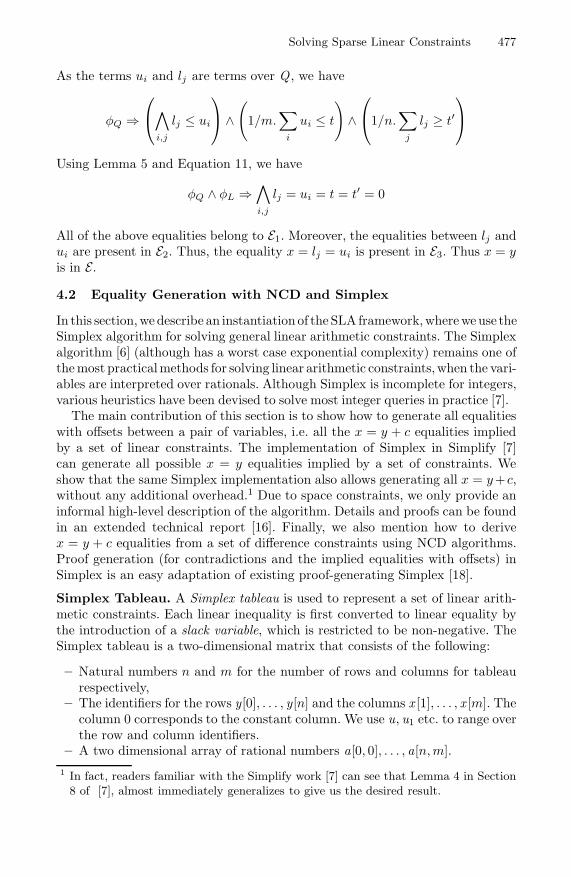
Solving Sparse Linear Constraints 477
As the terms ui and lj are terms over Q , we have
φQ ⇒
⎛
⎝∧
i,j
lj ≤ ui
⎞
⎠ ∧(
1/m.∑
i
ui ≤ t
)
∧
⎛
⎝1/n.∑
j
lj ≥ t′
⎞
⎠
Using Lemma 5 and Equation 11, we have
φQ ∧ φL ⇒∧
i,j
lj = ui = t = t′ = 0
All of the above equalities belong to E1. Moreover, the equalities between lj andui are present in E2. Thus, the equality x = lj = ui is present in E3. Thus x = yis in E.
4.2 Equality Generation with NCD and Simplex
In this section,wedescribe an instantiation of the SLA framework,whereweuse theSimplex algorithm for solving general linear arithmetic constraints. The Simplexalgorithm [6] (although has a worst case exponential complexity) remains one ofthe most practicalmethods for solving linear arithmetic constraints,when the vari-ables are interpreted over rationals. Although Simplex is incomplete for integers,various heuristics have been devised to solve most integer queries in practice [7].
The main contribution of this section is to show how to generate all equalitieswith offsets between a pair of variables, i.e. all the x = y + c equalities impliedby a set of linear constraints. The implementation of Simplex in Simplify [7]can generate all possible x = y equalities implied by a set of constraints. Weshow that the same Simplex implementation also allows generating all x = y+c,without any additional overhead.1 Due to space constraints, we only provide aninformal high-level description of the algorithm. Details and proofs can be foundin an extended technical report [16]. Finally, we also mention how to derivex = y + c equalities from a set of difference constraints using NCD algorithms.Proof generation (for contradictions and the implied equalities with offsets) inSimplex is an easy adaptation of existing proof-generating Simplex [18].
Simplex Tableau. A Simplex tableau is used to represent a set of linear arith-metic constraints. Each linear inequality is first converted to linear equality bythe introduction of a slack variable, which is restricted to be non-negative. TheSimplex tableau is a two-dimensional matrix that consists of the following:
– Natural numbers n and m for the number of rows and columns for tableaurespectively,
– The identifiers for the rows y[0], . . . , y[n] and the columns x [1], . . . , x [m]. Thecolumn 0 corresponds to the constant column. We use u, u1 etc. to range overthe row and column identifiers.
– A two dimensional array of rational numbers a[0, 0], . . . , a[n, m].1 In fact, readers familiar with the Simplify work [7] can see that Lemma 4 in Section
8 of [7], almost immediately generalizes to give us the desired result.

478 S.K. Lahiri and M. Musuvathi
– A subset of identifiers (representing the slack variables) in y[0], . . . , y[n],x [1], . . . , x [m] have a sign ∈ {≥, ∗}, and are called restricted. A variable uwith sign of ∗ is called ∗-restricted, and denotes that u = 0; otherwise arestricted variable u with sign ≥ denotes u ≥ 0.
– The y[0] of the Simplex tableau is a special row Zero to denote the value 0,and has 0 in all columns.
Each row in the tableau represents a row constraint of the form:
y[i] = a[i, 0] + Σ1≤j≤ma[i, j].x [j] (12)
A feasible tableau is one where the solution obtained by setting each of thecolumn variables x [j] to 0 and setting each of the y[i] to a[i, 0], satisfies allthe constraints (row constraints and sign constraints). A set of constraints issatisfiable iff such a feasible tableau exists. We will not go into the details offinding the feasible tableau, as it is a well-known method [6,7].
Equality Generation from Simplex Tableau. To generate equalities impliedby the set of constraints, the tableau has to be constrained further in additionto being feasible. The tableau has to be constrained such that for any restrictedvariable u, the set of constraints imply u = 0, if and only if u is ∗-restricted in thetableau. Such a tableau is called a minimal tableau. The Simplex implementationin Simplify [7] provides a procedure for obtaining a minimal tableau for a set ofconstraints. The set of all implied variable equalities (of the form u1 = u2) can besimply read off the minimal tableau. We show that, in fact, the set of all impliedoffset equalities (of the form u1 = u2 + c) can also be read off such a minimaltableau. The basic idea is that in a minimal tableau, the implied equalities donot depend on the ≥ sign constraints.
We now state the generalization of Lemma 2 (Section 8.2 [7]) to include offsetequalities:
Lemma 6 (Generalization of Lemma 2 in Section 8.2 [7]). For any twovariables u1 and u2 in a feasible and minimal tableau, the set of constraintsimply u1 = u2 + c, where c is a rational constant, if and only if at least one ofthe following conditions hold:
1. u1 and u2 are both ∗-restricted columns (here c is 0), or2. both u1 and u2 are row variables y[i] and y[j] respectively, and apart from
the ∗-restricted columns only (possibly) differ in the constant column, suchthat a[i, 0] = a[j, 0] + c, or
3. u1 is a row variable y[i], u2 is a column variable x [j], and the only non-zero entries in the row i outside the ∗-restricted columns are a[i, 0] = c anda[i, j] = 1.
4. u2 is a ∗-restricted column, and u1 is a row variable y[i], such that a[i, 0] = cis the only non-zero entry outside ∗-restricted columns in row i.
Therefore, obtaining the minimal tableau is sufficient to derive even x = y + cfacts from Simplex. This is noteworthy because the Simplex implementation doesnot incur any more overhead in generating these more general equalities thansimple x = y equalities.

Solving Sparse Linear Constraints 479
Inferring Equalities from NCD. The algorithm for SLA equality generationdescribed in Section 4.1 requires generating equalities of the form x = y+c fromthe NCD component of SLA. Lemma 2 in [15] provides such an algorithm. Thelemma is provided here.
Lemma 7 (Lemma 2 in [15]). For an edge e in Gφ representing y ≤ x + c, ecan be strengthened to represent y = x + c (called an equality-edge), if and onlyif e lies in a cycle of weight zero.
Hence, using Lemma 6, Theorem 2 and Lemma 7, we obtain a complete equalitygenerating decision procedure over rationals.
Theorem 3. The SLA implementation by combining NCD and Simplex is anequality generating decision procedure for linear arithmetic over rationals.
5 Implementation and Results
In this section, we describe our implementation of the SLA algorithm in theZap [1] theorem prover and report preliminary results from our experiments.The implementation uses the Bellman-Ford algorithm as the NCD algorithmand the Simplex implementation (described in Section 4.2) for the non-differenceconstraints. We are currently working on the implementation of the proof gen-eration from the SLA algorithm (namely, the proof of implied equalities fromNCD [15]) , to integrate it into the lazy proof-generating theorem prover frame-work [2,8]. Hence, we are currently unable to evaluate our algorithm on morerealistic benchmarks (such as the SMT-LIB benchmarks [26]), where we need theproofs to generate conflict clauses to reason about the Boolean structure in theformula. Instead, we evaluate on a set of randomly generated linear arithmeticbenchmarks.
We report preliminary results comparing our algorithm with two different im-plementations for solving linear arithmetic constraints: (i) Simplify-Simplex: thelinear arithmetic solver in the Simplify [7] theorem prover, and (ii) Zap-UTVPI:an implementation of Unit Two Variable Per Inequality (UTVPI) decision pro-cedure [10,12] in Zap.2 Even though Zap-UTVPI is not complete for generallinear arithmetic, we chose this implementation to compare a transitive closurebased decision procedure (as used by Sheini and Sakallah [25]) to a one basedon NCD algorithms.
We generated the random benchmarks as follows. For different values for thetotal number of variables lying between 100 and 1000, we generated benchmarkswith the number of constraints varying from half to five times the number ofvariables. To measure the effect of the sparseness of the constraints, we varied theratio of non-difference constraints to difference constraints from 2% to 50%. Foreach difference constraint we picked the two variables at random. For each non-difference constraint we randomly picked 2 to 5 variables and chose a random2 UTVPI constraints are of the form a.x + b.y ≤ c, where a and b ∈ {−1, 0, 1} and c
is an integer constant.

480 S.K. Lahiri and M. Musuvathi
Execution Times (secs)
0.01
0.1
1
10
100
1000
0.01 0.1 1 10 100 1000
SLA
Sim
plif
yExecution Times (secs)
0.01
0.1
1
10
100
1000
0.01 0.1 1 10 100 1000
SLA
UT
VP
I
Fig. 1. Comparison of SLA with (a) Simplify-Simplex and (b) Zap-UTVPI on a set ofrandomly generated benchmarks
coefficient between −2 and 2. We ensured that the set of benchmarks when runon the SLA implementation involved all of the following: instances where thedifference constraints alone were unsatisfiable, instances where the non-differenceconstraints alone were unsatisfiable, instances that required both difference andnon-difference reasoning, and finally instances that were satisfiable.
Figure 1 (a) shows the comparison of the execution times of the SLA algo-rithm against Simplify-Simplex. In the graph, we indicate both the runs thattook greater than 200 seconds and runs that incurred a crash due to an integer-overflow exception, as timeouts with 200 seconds. The overflow exception hap-pens in Simplex (both in Simplify and Zap) due to the use of machine integersto represent large coefficients in the tableau. The following observations are ev-ident from this graph. On those instances for which Simplify finished within asecond, the SLA algorithm also finished within a second, but performed worsethan Simplify. This is a result of the constant overhead Zap (implemented inC#) incurs loading the virtual machine of the C# language on every run. Onthe other hand, SLA solved instances within seconds for which Simplify requiredorders of magnitude longer time or timed out at 200 seconds. To our surprise,Simplify incurred an integer-overflow exception on many benchmarks for whichpure difference reasoning was sufficient to prove the unsatisfiability of the query.The SLA implementation did incur an integer-overflow on certain instances forwhich Simplify completed successfully. This could be due to the fact that ourSimplex implementation is not as optimized as the one in Simplify as we havenot implemented the many pivot heuristics of Simplify.
Figure 1 (b) shows the execution time of the UTVPI decision procedure onthese benchmarks. SLA performs better than the UTVPI decision procedure ona greater proportion of the instances. The transitive-closure based algorithm forthe UTVPI decision procedure has a quadratic space complexity, resulting inorders of magnitude slowdown. There are instances, however, where the SLAalgorithm results in an integer-overflow for which the UTVPI algorithm termi-nates. (Note, the UTVPI algorithm is incomplete for general linear arithmetic.)This suggests a possibility of combining the linear-space UTVPI algorithm [14]with a general linear arithmetic solver, along the lines of SLA. While this is aninteresting problem for future work, we are unsure about its value in practice.
Solving Sparse Linear Constraints 481
6 Related Work
Checking the satisfiability of a set of linear arithmetic constraints over integersis NP-complete [20]. Various algorithms based on branch-and-bound heuris-tics are implemented in various integer linear programming (ILP) solvers likeLP SOLVE [17] and commercial tools like CPLEX [11] to solve this fragment.These algorithms have a worst-case exponential time complexity. Even for therelaxation of the linear arithmetic problem over rationals (where polynomialtime decision procedures exists [13]), most practical solvers use Simplex [6] al-gorithm that has a worst-case exponential complexity. Gomory cuts [23] canbe used to extend Simplex over integers although the algorithm might requireexponential space in the worst case. Ruess and Shankar [22] provide one suchimplementation. Their algorithm also generates equalities over variables. How-ever, unlike our approach, their algorithm does not try to exploit the sparsity inlinear arithmetic constraints, and the asymptotic complexity for solving sparselinear arithmetic constraints is still exponential.
Recently attempts have been made to exploit the sparsity in linear arithmeticconstraints mostly dominated by difference logic queries. Seshia and Bryant [24]demonstrate that although one might incur a linear blowup for translating aBoolean formula over linear arithmetic constraints (over integers) to an equisatis-fiable propositional formula, formulas with only a small number of non-differenceconstraints can be converted using a logarithmic blowup. This approach how-ever does not help towards improving the complexity of solving a set of lineararithmetic constraints.
The closest approach to ours is the approach of Sheini and Sakallah [25], wherethey provide a decision procedure for integer linear arithmetic by combining adecision procedure for UTVPI constraints and a general linear arithmetic solver(CPLEX [11] in their case). Their algorithm relies on computing a transitiveclosure for the UTVPI constraints that incurs cubic time and quadratic spacecomplexity, independent of the sparsity of the constraints. In contrast, our de-cision procedure retains the efficiency of the NCD algorithms thereby makingour procedure robust even for non sparse linear arithmetic benchmarks. This iswell demonstrated by our experimental results (Figure 1 (b)). Moreover, theircombination does not generate models for satisfiable formulas. Finally, their al-gorithm does not provide a way to generate implied equalities that are crucialfor a Nelson-Oppen framework.
References
1. T. Ball, S. K. Lahiri, and M. Musuvathi. Zap: Automated theorem proving forsoftware analysis. In Logic for Programming, Artificial Intelligence, and Reasoning(LPAR 2005), LNCS 3835, pages 2–22, 2005.
2. C. W. Barrett, D. L. Dill, and A. Stump. Checking satisfiability of first-order for-mulas by incremental translation to SAT. In CAV 02: Computer-Aided Verification,LNCS 2404, pages 236–249, 2002.
3. R. Bellman. On a routing problem. Quarterly of Applied Mathematics, 16(1):87–90,1958.

482 S.K. Lahiri and M. Musuvathi
4. B. V. Cherkassky and A. V. Goldberg. Negative-cycle detection algorithms. InEuropean Symposium on Algorithms, pages 349–363, 1996.
5. T. H. Cormen, C. E. Leiserson, and R. L. Rivest. Introduction to Algorithms. MITPress, 1990.
6. G. Dantzig. Linear programming and extensions. Princeton University Press,Princeton NJ, 1963.
7. D. L. Detlefs, G. Nelson, and J. B. Saxe. Simplify: A theorem prover for programchecking. Technical report, HPL-2003-148, 2003.
8. C. Flanagan, R. Joshi, X. Ou, and J. Saxe. Theorem proving using lazy proofexplication. In CAV 03: Computer-Aided Verification, LNCS 2725, pages 355–367,2003.
9. L. R. Ford, Jr., and D. R. Fulkerson. Flows in Networks. 1962.10. W. Harvey and P. J. Stuckey. A unit two variable per inequality integer constraint
solver for constraint logic programming. In Proceedings of the 20th AustralasianComputer Science Conference (ACSC ’97), pages 102–111, 1997.
11. ILOG CPLEX. Available at http://ilog.com/products/cplex.12. J. Jaffar, M. J. Maher, P. J. Stuckey, and H. C. Yap. Beyond finite domains. In
PPCP 94: Principles and Practice of Constraint Programming, LNCS 874, pages86–94, 1994.
13. Narendra Karmarkar. A new polynomial-time algorithm for linear programming.Combinatorica, 4(4):373–396, 1984.
14. S. K. Lahiri and M. Musuvathi. An efficient decision procedure for UTVPI con-straints. In FroCos 05: Frontiers of Combining Systems, LNCS 3717, pages 168–183, 2005.
15. S. K. Lahiri and M. Musuvathi. An Efficient Nelson-Oppen Decision Procedurefor Difference Constraints over Rationals. Number 2 in ENTCS 144, pages 27—41,2005.
16. S. K. Lahiri and M. Musuvathi. Solving sparse linear constraints. Technical ReportMSR-TR-2006-47, Microsoft Research, 2006.
17. LP SOLVE. Available at http://groups.yahoo.com/group/lp solve/.18. G. C. Necula and P. Lee. Proof generation in the touchstone theorem prover. In
Conference on Automated Deduction, LNCS 1831, pages 25–44, 2000.19. G. Nelson and D. C. Oppen. Simplification by cooperating decision procedures.
ACM Transactions on Programming Languages and Systems (TOPLAS), 2(1):245–257, 1979.
20. C. H. Papadimitriou. On the complexity of integer programming. J. ACM,28(4):765–768, 1981.
21. V. Pratt. Two easy theories whose combination is hard. Technical report, Mas-sachusetts Institute of Technology, Cambridge, Mass., September 1977.
22. H. Rueß and N. Shankar. Solving linear arithmetic constraints. Technical ReportCSL-SRI-04-01, SRI International, January 2004.
23. A. Schrijver. Theory of Linear and Integer Programming. Wiley, 1986.24. S. A. Seshia and R. E. Bryant. Deciding quantifier-free Presburger formulas using
parameterized solution bounds. In LICS 04: Logic in Computer Science, pages100–109, July 2004.
25. H. M. Sheini and K. A. Sakallah. A scalable method for solving satisfiability ofinteger linear arithmetic logic. In Theory and Applications of Satisfiability Testing(SAT 2005), LNCS 3569, pages 241–256, 2005.
26. SMT-LIB: The Satisfiability Modulo Theories Library. Available athttp://combination.cs.uiowa.edu/smtlib/.


![Approximate Lie Group Analysis of Finite–difference Equations · Approximate Lie Group Analysis of Finite–difference Equations A.M.Latypov ... Levi and Winternitz [8] applied](https://img.dokumen.tips/doc/110x75/5edcb4acad6a402d66677c2b/approximate-lie-group-analysis-of-finiteadiierence-equations-approximate-lie.jpg)