Solar PV GRID-TIED SYSTEM I: A CASE STUDY IN K.S.A

APPLYING A PV GRID-TIED SYSTEM IN INDUSTRIAL SECTOR WITH

PAYBACK REDUCTION: A CASE STUDY IN K.S.A.

by

Wayel Khaled Oweedha

Submitted in partial fulfillment of the requirements

for the degree of Master of Applied Science

at

Dalhousie University Halifax, Nova Scotia

April 2013

© Copyright by Wayel Khaled Oweedha, 2013

DALHOUSIE UNIVERSITY

DEPARTMENT OF ELECTRICAL AND COMPUTER ENGINEERING

The undersigned hereby certify that they have read and recommend to the Faculty of

Graduate Studies for acceptance a thesis entitled “Applying a PV Grid-Tied System in

Industrial Sector with Payback Reduction: A Case Study in K.S.A.” by Wayel Khaled

Oweedha in partial fulfillment of the requirements for the degree of Master of Applied

Science.

Dated: April 10, 2013

Supervisor: ______________________________

Readers: ______________________________

______________________________

DALHOUSIE UNIVERSITY

DATE: April 10, 2013

AUTHOR: Wayel Khaled Oweedha

TITLE: Applying a PV Grid-Tied System in Industrial Sector with Payback Reduction: A Case Study in K.S.A.

DEPARTMENT:

DEGREE: MASc CONVOCATION: October YEAR: 2013

Permission is herewith granted to Dalhousie University to circulate and to have copied for non-commercial purposes, at its discretion, the above title upon the request of individuals or institutions. I understand that my thesis will be electronically available to the public. The author reserves other publication rights, and neither the thesis nor extensive extracts from it may be printed or otherwise reproduced without the author’s written permission. The author attests that permission has been obtained for the use of any copyrighted material appearing in the thesis (other than the brief excerpts requiring only proper acknowledgement in scholarly writing), and that all such use is clearly acknowledged.

.

_______________________________ Signature of Author

Dedicated

To my family & my parents

TABLE OF CONTENTS

LIST OF TABLES ........................................................................................................... viii

LIST OF FIGURES ............................................................................................................ x

ABSTRACT ...................................................................................................................... xii

LIST OF ABBREVIATIONS AND SYMBOLS USED ................................................. xiii

ACKNOWLEDGEMENTS ............................................................................................. xiv

CHAPTER 1: INTRODUCTION ....................................................................................... 1

1.1 General ................................................................................................................... 1

1.2 Motivation .............................................................................................................. 1

1.3 Objective ................................................................................................................ 3

1.4 Thesis Outline ........................................................................................................ 3

CHAPTER 2: SOLAR ENERGY ....................................................................................... 5

2.1 Solar Energy .......................................................................................................... 5

2.1.1 Solar Thermal System ..................................................................................... 6

2.1.2 Solar Photovoltaic Technology (PV) .............................................................. 6

2.2 Solar Photovoltaic Technology (PV) ..................................................................... 7

2.2.1 Solar Cells ....................................................................................................... 7

2.3 Classification of PV Systems ............................................................................... 13

2.3.1 Stand-Alone or Off-Grid System .................................................................. 13

2.3.2 Grid-Connected or Grid-Tied System ........................................................... 14

2.3.3 Typical System Components ......................................................................... 15

CHAPTER 3: USING SOLAR ENERGY IN SAUDI ARABIA .................................... 18

3.1 Saudi Arabia's Locatin ......................................................................................... 18

3.2 Saudi Arabia and Solar Energy ............................................................................ 19

3.3 Power Consumption in Saudi Arabia .................................................................. 19

3.4 Electricity Price (Tariff and Feed in Tariff): ........................................................... 20

3.4.1 The Tariff ...................................................................................................... 20

3.4.2 Feed-in-Tariff: ............................................................................................... 21

3.5 The Industrial Sector in Saudi Arabia ................................................................. 22

3.6 PV System Applications in Saudi Arabia ............................................................ 23

CHAPTER 4: METHODOLOGY .................................................................................... 32

4.1 HOMER Software ............................................................................................... 32

4.2 How the Software Works ..................................................................................... 33

4.2.1 The Load ........................................................................................................ 34

4.2.2 System Components ...................................................................................... 35

4.2.3 Grid Input ...................................................................................................... 35

4.2.4 Solar Resource Input ..................................................................................... 36

4.2.5 Temperature Input ......................................................................................... 37

4.2.6 The Economic Input ...................................................................................... 37

4.2.5 Constraints ..................................................................................................... 39

4.2.6 Simulation and Results .................................................................................. 38

4.3 Input Data ............................................................................................................ 41

4.3.1 The Factory Load .......................................................................................... 41

4.3.2 The Temperature of the City ......................................................................... 43

4.3.3 Solar Equipment Specifications .................................................................... 44

4.3.4 The Grid Information ....................................................................................... 45

4.3.5 Solar Resource ............................................................................................... 48

4.3.6 Economic Entries .......................................................................................... 47

4.3.7 Constraints ..................................................................................................... 48

4.6 The Economic Calculation .................................................................................. 49

4.6.1 Introduction ................................................................................................... 49

4.6.2 Economic Factors .......................................................................................... 49

4.6.3 Net Present Value and Future Worth ............................................................ 52

4.6.4 Life Cycle Cost (LCC) .................................................................................. 51

4.6.5 Internal Rate of Return (IRR) ........................................................................ 54

4.6.6 Payback Period (PB) ..................................................................................... 55

CHAPTER 5: RESULTS AND DISCUSSION ................................................................ 56

5.1 The Output Result ................................................................................................ 56

5.2 Sensitivity Analysis ............................................................................................. 60

5.2.1 First Scenario ................................................................................................. 60

5.2.2 Second Scenario ............................................................................................ 71

5.3 The Effects on Payback Period ............................................................................ 81

5.3.1 The Load ........................................................................................................ 81

5.3.2 Subsidy by the Saudi Arabia Government: ................................................... 85

CHAPTER 6: CONCLUSIONS, RECOMMENDATIONS AND FUTURE WORK. .... 89

6.1 Conclusion ........................................................................................................... 89

6.2 Contribution ..................................................................................................... 90

6.3 Recommendations ............................................................................................ 90

6.4 Future work ........................................................................................................... 91

APPENDIX A: PV System Price ...................................................................................... 92

APPENDIX B: Technical Data for PV System Component ............................................ 93

Bibliography ..................................................................................................................... 95

LIST OF TABLES

Table (4-1): The monthly factory load. ............................................................................. 40

Table (4-2): The PV kit price. ........................................................................................... 43

Table (4-3): The inverter price. ......................................................................................... 44

Table (5-1): Grid only system electricity consumption. ................................................... 56

Table (5-2): The PV system size and cost. ....................................................................... 58

Table (5-3): Electrical data from the simulation. .............................................................. 59

Table (5-5): Scenario (1) system size and cost for system (1). ......................................... 61

Table (5-6): Scenario (1) Electrical detail for system (1). ................................................ 61

Table (5-7): Scenario (1) Economic analysis for system (1). ........................................... 62

Table (5-9): Scenario (1) Electrical detail for system (3). ................................................ 64

Table (5-10): Scenario (1) Economic data for the system (2). ......................................... 64

Table (5-11): Scenario (1) size and cost for system (3). ................................................... 65

Table (5-12): Scenario (1), Economic analysis for system (3). ........................................ 66

Table (5-13): Scenario1, Economic data for the system (3). ............................................ 66

Table (5-14): Scenario (1), the summary table for scenario (1). ...................................... 66

Table (5-15): Scenario (1), economic calculation. ............................................................ 68

Table (5-17): Scenario (1), the payback for system (1). ................................................... 69



Table (5-20): Scenario (2) system (1) size and cost. ........................................................ 71

Table (5-21): Scenario (2) Electrical data for system (1). ................................................ 72

Table (5-22): Scenario 2 Economic data for system (1). .................................................. 72

Table (5-23): Scenario (2) system (2) size and cost. ........................................................ 72

Table (5-24): Scenario (2) Electrical data for system (2). ................................................ 73

Table (5-25): Scenario (2) Economic data for system (2). ............................................... 73

Table (5-26): Scenario (2), PV system size and cost for system (3). ................................ 74

Table (5-27): Scenario (2), Electrical data for system (3). ............................................... 75

Table (5-28): Scenario (2), Economic results for system (3). ........................................... 75

Table (5-29): summary results for the second scenario. ................................................... 75

Table (5-30): The economic calculation for the second scenario. .................................... 76


Table (5-33): Scenario (2), the payback for system (2) .................................................... 77

Table (5-34): Scenario 2 the IRR for the systems. ............................................................ 79

Table (5-35): The optimal system specification. .............................................................. 81

Table (5-36): Load change. ............................................................................................... 82

Table (5-37): The payback vs. load change. ..................................................................... 84

Table (5-38): The government subsidy table. ................................................................... 85

Table (5-39): The payback with 10% government subsidy. ............................................. 86



Table (5-42): The final PV system cost. ........................................................................... 88

LIST OF FIGURES

Figure (1-1): Peak load in Saudi Arabia [3] ........................................................................ 2

Figure (2-1) Silicon atoms [12] ........................................................................................... 8

Figure (2-2): The Depletion region [12] ............................................................................. 9

Figure (2-3): Photovoltaic system [16] ............................................................................. 10

Figure (2-4): Types of crystalline silicon solar sell .......................................................... 13

Figure (2-5): Stand-alone system [22] .............................................................................. 14

Figure (2-6): Grid-tied system [23] ................................................................................... 15

Figure (2-7): Components of PV array [24] ..................................................................... 16

Figure (3-1): Average daily solar radiation [28] ............................................................... 19

Figure (3-2): The industrial cities in Saudi Arabia [33] ................................................... 23

Figure (4-1): HOMER configuration [49]. ....................................................................... 33

Figure (4-2): HOMER main window. ............................................................................... 34

Figure (4-3): The components cost and range [49]. .......................................................... 35

Figure (4-4): HOMER Grid window. ............................................................................... 35

Figure (4-5): HOMER solar resource window. ................................................................ 36

Figure (4-6): HOMER temperature window. .................................................................... 37

Figure (4-7): HOMER economic window. ....................................................................... 37

Figure (4-8): HOMER constraints window. ..................................................................... 38

Figure (4-9): HOMER results window. ............................................................................ 39

Figure (4-10): HOMER optimization result. ................................................................... 39

Figure (4-11): The Factory load. ....................................................................................... 41

Figure (4-12): The Factory Load in HOMER. .................................................................. 42

Figure (4-13): Jeddah temperature detail in HOMER. ..................................................... 42

Figure (4-14): The PV detail and cost entered in HOMER. ............................................. 44

Figure (4-15): The PV detail and cost entered in HOMER. ............................................. 45

Figure (4-16): First scenario grid rate schedule. ............................................................... 46

Figure (4-17): Second scenario grid rate schedule. .......................................................... 46

Figure (4-18): Solar radiation and clearness index. .......................................................... 47

Figure (4-19): The economic information. ....................................................................... 48

Figure (4-20): The fraction covered by PV system. ......................................................... 48

Figure (4-21): System configuration. ................................................................................ 49

Figure (5-1): The monthly average electricity. ................................................................. 56

Figure (5-2): The over all result from the HOMER. ......................................................... 57

Figure (5-3): The optimization systems result. ................................................................. 58

Figure (5-4): Scenario (1), the optimal result for system (1). ........................................... 60

Figure (5-5): The monthly average electric production for system (1). ........................... 60

Figure (5-6): Scenario (1), the optimal result for system (2). ........................................... 62

Figure (5-7): The monthly average of electric production for system (2). ....................... 63

Fig (5-8): Scenario (1), the optimal result for system (3). ................................................ 64

Figure (5-9): The monthly average electrical production. ................................................ 65

Figure (5-10): Scenario (2), the optimal result for system (3). ......................................... 73

Figure (5-11): Scenario (2) the monthly average for system (3). ..................................... 74

Figure (5-12): The payback for senior (2) for all systems. ............................................... 78

Figure (5-13): The power purchase from the grid. ........................................................... 80

Figure (5-14): Load change by ± 5%. ............................................................................... 82

Figure (5-15): Load change by ± 25%. ............................................................................. 83

Figure (5-16): The payback for load change by 5%. ........................................................ 83

Figure (5-17): The payback for load change by 25%. ...................................................... 84

Figure (5-18): Payback VS load. ...................................................................................... 85

Figure (5-19): The Payback VS. Subsidy. ........................................................................ 87

Figure (5-20): The payback for the final system. ............................................................. 88

ABSTRACT

The key to creating clean energy is to use renewable energy sources. Saudi Arabia has an abundance of solar radiation due to its geographical location; therefore, solar energy applications provide excellent opportunities for generating electricity in the region. Since 1960, Saudi Arabia has examined potential photovoltaic (PV) applications however, the progress towards implementing a solar energy program has not been sufficient. In Saudi Arabia, the industrial sector consumes a large portion of the power load demand. The biggest industrial cities in Saudi Arabia are Dammam, Al-Jubile, Jeddah, and Riyadh. This study examines the potential application of solar energy through a PV system in the Saudi Arabian industrial sector. The research seeks to examine whether a PV system combined with a grid system could be feasible to apply in the country. To examine this, a typical energy consumption daily profile is assumed. The study uses an existing factory in the city of Jeddah for simulation. HOMER and Microsoft Excel are used to carry out the study. Furthermore, the economic reliability and feasibility of the examined results will be included. Finally ways to reduce the payback time was investigated and a cost effective system is recommended. Index Terms – Industrial area, Saudi Arabia, Solar system, PV system, Renewable energy.

LIST OF ABBREVIATIONS AND SYMBOLS USED

PV

a-Si

Photovoltaic

Amorphous Silicon

FIT Feed-in-Tariff

GSR Global Solar Radiation

GOIC Gulf Organization for Industrial Consulting

KACST King Abdulaziz City for Science and Technology

RETscreen Renewable Energy Technology Screen

HOMER Hybrid Optimization Model for Electric Renewable

i The Discount Rate

CRF The Capital Recovery Factor

NPC Net Present Cost

COE Cost of Energy

P Present Worth

F Future Worth

LCC Life Cycle Cost

LEC Levelized Energy Cost

E The Annual Energy

IRR Internal Rate of Return

PB Payback Period

ACKNOWLEDGEMENTS

In the name of Allah Almighty and the merciful thanks be to Allah for helping me

achieve my degree.

I would like to show my deepest gratitude and respect to King Abdullah

(Custodian of the Tow Holy Mosques) for his kindness and generosity in granting me a

scholarship and supporting my studies to pursue my Master’s degree.

I would like to express my gratitude towards my supervisor Dr. Mohammad El-

Hawary for his guidance, encouragement and continuous support during the course of my

graduate study. His deep insight and extensive knowledge were very inspirational and

helpful towards the successful completion of my degree. I would like to thank Dr.

William J. Phillips and Dr. Jason Gu for their valuable suggestions in improving the

quality and readability of this thesis also for being in my supervisory committee.

I extend special thanks to my parents for their love and support throughout my

life. Thank you both for giving me strength to reach for the stars and chase my dreams.

Finally, words cannot express how grateful I am to my family. When I think of my

family, I think of love. Special thanks to my wife, Waud, the mother of my children

(Miral and Qusai), for her support and encouragement..

CHAPTER 1 INTRODUCTION

1.1 General

The Kingdom of Saudi Arabia (KSA) is blessed with an abundance of energy resources.

KSA currently holds the largest oil reserve in the world and is also rich in gas reserves,

and has great potential for wind and solar energy. KSA is currently the world’s 20th

largest producer and consumer of electricity. The country’s geographical location

includes a photovoltaic (PV) area of 22 – 40 km2 and can produce as much electricity as a

1000 MWe oil-fired power station. This advantage can potentially make electricity

generated from PV systems more competitive than electricity generated from oil-fired

power generation [1].

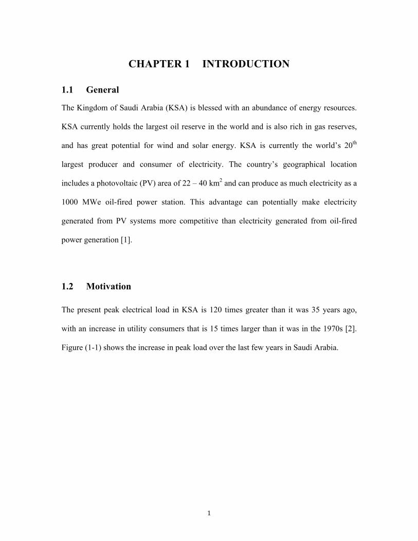
1.2 Motivation

The present peak electrical load in KSA is 120 times greater than it was 35 years ago,

with an increase in utility consumers that is 15 times larger than it was in the 1970s [2].

Figure (1-1) shows the increase in peak load over the last few years in Saudi Arabia.

Figure (1-1): Peak load in Saudi Arabia [3]

The fast growing population, high economic growth, and low utility tariffs are

some of the many factors playing a role in and fueling this increase in power demand. In

addition to the increasing population and increase in the power utility consumers, KSA

needs to expand its electronic power transmission network and generation capability to

support its motivated industrialization plan [2].

Following residential load, the industrial sector is the highest consumption sector

in Saudi Arabia. The industrial sector industries in Saudi Arabia consist of

petrochemicals, oil refining, steel and iron, cement and other industries. The average

growth rate in the industrial sector is 4.3%. In 2008 the energy consumption of the

industrial sector in Saudi Arabia reached 150 TWh [1]. Present reports confirm the

industrial sector is currently consuming 18% of the country’s total energy consumption

[4].

Jeddah is one of the cities facing a current overload in industrial power demands.

The Saudi electricity utility recently informed industries that it might need to cut back on

the amount of power supplied to the industrial sector during peak hours. The government

has reported that this decrease will help avoid any massive power outages in the city. A

power reduction in the industrial sector will not only affect business, but it could

potentially cause damage to certain machinery used in the sector. This alarming issue has

motivated the industrial sector to develop a solution [5].

1.3 Objective

The main goal of this thesis is to find a renewable energy solution by supplementing the

grid source with a PV system and potentially selling any excess power generated by the

PV system back to the grid during peak hours. An economic study of the cost and

economic payback will determine if the application of this method is cost effective and

efficient.

1.4 Thesis Outline

This thesis will begin with a brief discussion of the nature of solar energy and PV

systems in Chapter 2. Some general definitions and terms will also be discussed in this

chapter.

Chapter three will deal with weather conditions in Saudi Arabia and present the

climatic reasons that make Saudi Arabia’s geographic location optimal for the application

of solar energy.

Chapter four will present the methodology used to generate the optimal

application methods and will discuss the use of HOMER, Excel, and economic

calculations used to support the results.

Chapter five will present the results and a brief discussion of the optimal solution.

Chapter six will offer a brief conclusion and will suggest some future work that could be

applied to further develop the application of solar energy in KSA.

CHAPTER 2: SOLAR ENERGY

This chapter presents a literature review intended to provide a background understanding

of the concepts of PV systems and PV system types. A short background to solar energy

and the types of solar systems is also provided.

2.1 Solar Energy

The history of solar energy technology dates back to more than one hundred and fifty

years ago. The term solar energy refers to any source of energy that is directly obtained

from sunlight or the heat that the sunlight generates. Solar energy is a renewable source

of energy.

Technology to exploit solar energy has been developed since 1860. At that time,

solar energy was used to capture the sun’s heat and generate steam, which would enable

activities like running engines and irrigation pumps. This technology has recently

undergone a drastic growth. The direct consequence has been relevant cost reductions for

the use of solar energy. There has also been an increase in government support to

implement solar energy due to its renewable nature and the fact that it is environmentally-

friendly [6].

Reaching up to 0.06W/m2 of irradiance on the earth’s surface at the highest

latitudes and 0.25kW/m2 at the lowest, solar energy represents by far the largest source of

renewable energy known today [6].

The following subsections explain a classification of the various solar energy

technologies.

2.1.1 Solar Thermal System

To generate solar thermal power, the sun is exploited as a source of heat. The heat is

concentrated and used to generate power by means of a heat engine. This method reflects

the traditional forms of power generation, which are based on fossil-fuel combustion and

which also generate electrical energy from the heat produced by the heat engine.

Currently, the technologies employed to produce solar thermal power are categorized in

a) parabolic trough systems, b) solar tower systems, and c) solar dish systems. The

distinction is based on the way these systems concentrate solar radiation [7].

2.1.2 Solar Photovoltaic Technology (PV)

The term “photovoltaic” is composed of the words “photo”, which stems from the Greek

“light”, and “voltaic”, which indicates electricity. The purpose of PV is to convert

sunlight directly into electricity, with an efficiency that currently reaches to 12-19%

when the conditions are best [8, 9]. PV use is very common in houses, residential or

commercial buildings, telecommunication industries, work in rural areas, etc. This source

of electrical power was considered after the 1973 fuel crisis [10].

Current predictions indicating an upcoming shortage in gasoline and petroleum

has increased interest in PV technology. Consequently, this alternative form of energy

conversion has become a crucial element in most renewable energy programs [10]. PV

modules are becoming more present on roofs and facades [11] in developed countries.

The following section will discuss the ways that solar PV technology has recently

begun to grow and has attracted international government support, turning it into a non-

renounceable component of the 21st century energy mix.

2.2 Solar Photovoltaic Technology (PV)

The term photovoltaic applies to all devices or materials that, through the smallest

complete and environmentally protected assembly of connected solar cells, are able to

convert the energy contained in photons of light into electrical voltage [12]. As a future

energy technology, PV has the advantage of producing electricity silently without

producing harmful waste products [10]. Their convenience also lies in the fact that they

require very little maintenance, given the absence of moving parts wearing down the

device. This enables them to operate for many years on end. Their modularity allows

producers to obtain generators of any size or voltage by assembling varying numbers of

standard modules. This assembly is built to convert solar energy into electricity for some

specific purposes. The latter are met either alone or in combination with further energy

suppliers. Solar cells play a critical role in the conversion of solar energy into electrical

energy [13].

2.2.1 Solar Cells

Solar cells are semiconductor devices generating electricity exactly the moment light falls

on them [8]. Solar cells can also be called photovoltaic cells. Currently, PV devices are

generated starting from pure crystalline silicon, although their main technology is closely

related to the technology used to produce transistors, diodes, and all the semiconductor

devices widely used nowadays in the world [12]. As shown in Figure (2-1), the atomic

number for silicon is 14, with each atom having 14 negatively charged electrons orbiting

around a positively charged nucleus. Only ten of these electrons revolve tightly against

the nucleus, whereas the remaining four, which are not tightly bound to it, are the ones

playing the crucial role in PV systems. This bond can in fact be broken if sufficiently

jolted by an external source of heat or light [14]. Silicon is not an insulator (like glass) or

a conductor (like copper); silicon stands in the middle between the two.

+14 +4

(a) Actual (b) Simplified

Valenceelectrons

Figure (2-1) Silicon atoms [12]

However, a single and pure silicon wafer will never produce electricity, even if

placed in strong and direct sunlight. It is necessary for it to be connected to a mechanism

propelling electrons and holes in opposing directions in the crystal lattice. The current

therefore produces power by being forced through an external circuit. The mechanism

mentioned above is provided by the semiconductor p-n junction [14]. In order to make

the latter, the cell, which has two layers of silicon, has its layers doped with impure

atoms. Phosphorus is often added since, when doped with silicon, it generates a large

number of free atoms. These are known as majority carriers. Minority carriers are also

present in the shape of thermal-generated electron-hole pairs. This material makes an

excellent conductor and is mentioned as negative type, or n-type. If the silicon is doped

with boron, then other holes are created from broken bonds into the crystal; the situation

is reversed with respect to phosphorus, and the holes become the majority carriers while

the electrons are the minority carriers. This type of conductor is referred to as n–type, or

p-type [15].

While the doped material gathers to form a p-n junction and the free electrons that

are in the n-type material diffuse into the p-side, the hole in p-type diffuses in the n-side.

By doing this, they respectively leave behind two layers that are positively and negatively

charged. This diffusion of the materials in opposite directions across the interface is what

creates a strong electric field representing a potential barrier to further flow. The

diffusion continues until the electrons and holes come to a condition of balance; when

this occurs, charge carriers are no longer close to the junction, but they form what is

called “depletion region” as shown in Figure (2-2) [15].

p n

+

+

+

+

+

+

+

+

+

−+

−+

−+

+−

+−

+

−+

−+

−+

p n

+

+

+

+

+

+

+

+

+

−+

−+

−+

−+

−+

−+

Immobilenegativecharges

Immobilepositive charges

Mobileholes

Mobileelectrons

JunctionDepletionregion

Electric field

− − −

−−−

− − −

− − −

−

−

−−

− −

Figure (2-2): The depletion region [12]

At this point, the current flows in one direction because the p-n junction in the

depletion region acts like a diode. The electrons use the energy coming from the sun, in

the form of packets of energy termed photons, to free themselves from their nucleus.

Hitting the solar cell, the photons are powerful enough to create hole-electron pairs and

the resulting voltage will deliver the current to the load as shown in Figure (2-3) [12].

Figure (2-3): Photovoltaic system [16]

The former amounts to the percentage of solar radiation converting into electric

energy; the latter, instead, is usually lower than the cell efficiency because the module

also includes the frame and its surface cannot be fully covered with solar cells. The

highest efficiency for crystalline silicon cells is obtained when they operate in strong

sunlight [15].

Crystal silicon solar cells in the current high volume production can be divided

into three types:

2.2.1.1 Monocrystalline Silicon

Monocrystalline silicon, also known as single-crystal silicon, is the most common solar

cell semiconductor and the most promising in terms of high efficiency performance, as

shown in Figure (2-4 a). The highly efficient performance is a result of the abundance of

the material itself. The superior optical absorption coefficient makes it optimal for thin

film solar cells, with a cell thickness of < 1/xm. Its low costs are also widely

advantageous. Its low raw material requirements and low production energy requirements

provide cost-effective fabrication. Particularly, cost efficiency is what modeled solar cells

research toward developing single crystal ribbon silicon, which is also higher in quality.

Today in fact, the best single crystal Si solar cells can provide 24.7% efficiency in the

laboratory, while the conversion efficiency of commercial solar cell modules only

reaches up to 18% [8].

2.2.1.2 Polycrystalline Silicon

Unlike Monocrystalline silicon, polycrystalline cells consist of small particles of single-

crystal silicon as shown in Figure (2-4b). Polycrystalline PV cells are less efficient than

monocrystalline silicon with a lower (10-14%) energy conversion efficiency. This occurs

due to the flow of electrons being huddled by the grain boundaries; thus the cell power

output is inevitably reduced. Differing approaches are nowadays commonly employed to

produce polycrystalline silicon PV cells. One is to cut thin slices off blocks of cast

polycrystalline silicon, or to directly grow silicon as ribbons (“ribbon growth” method)

that are thick enough to make PV cells. EFG (the edge-defined film-fed growth) is the

most common and best developed “ribbon growth” approach. Polycrystalline silicon has

the advantage, unlike single-crystalline silicon, of being strong enough to be sliced into

one-third the thickness of single-crystalline silicon, with lower costs and fewer growth

requirements than single-crystal modules [8].

2.2.1.3 Amorphous Silicon (a-Si)

Amorphous silicon was discovered in 1974. The main characteristic of this non-

crystalline form of silicon is the disorderly structure of its atoms. PV modules produced

with this type of silicon were the first with a thin film produced at a commercial level as

shown in Figure (2-4 c). Currently, amorphous silicon provides the only thin film

technology casting a solid influence on PV markets. Its high sunlight absorbability being

40 times higher than that of single-crystal silicon represents its primary advantage. In

other words, using one thin layer of amorphous silicon it is possible to produce PV cells

that are 200 times thinner than those obtained with crystalline silicon (1μm compared

with 200 μm). Another remarkable advantage is the possibility of placing a-Si on low-

cost substrates made of steel, glass, and plastic due to the much lower temperatures

necessary for the manufacturing process. As a result, lower costs per unit area make a-Si

significantly more convenient than producing crystalline silicon cells [8].

a: Moncrystalline silicon[17]. b:Polycrystalline silicon [18]. c:Amorphous silicon[19].

Figure (2-4): Types of crystalline silicon solar cells

2.3 Classification of PV Systems

Photovoltaic systems can be generally classified into two main categories:

2.3.1 Stand-Alone or Off-Grid System

In this self-contained and cost-effective system, PV energy is converted to AC power

without being connected to a utility grid. This is a characteristic of all off-grid systems.

Off-grid systems have an inverter that regulates the AC voltage to all the loads. Most

stand-alone PV systems also require batteries to store the produced energy. This is

necessary since PVs can provide power during the daylight hours only. Energy storage is

thus required when the sun is not shining [12]. A charge controller prevents battery

overcharging and excess discharging, regulating the current that flows into the battery

bank from the PV array and then into the various electrical loads. While overcharging is

prevented by disconnecting the PV input whenever the battery voltage comes to an upper

set point, excess discharge can be avoided by simply disconnecting the load. It is also

possible to give a warning when the voltage falls to a lower set level [20]. In Figure (2-5)

the constituent elements of the system are a PV module, a controller, an inverter, and a

battery [21].

Figure (2-5): Stand-alone system [22]

.3.2 Grid-Connected or Grid-Tied System

Unlike off-grid systems, grid-tied systems have the power sent directly into the utility

grid if the system does not require power. The electricity automatically flows back and

forth according to electricity demands and sunlight conductions. In this system, the PV

array can be mounted on a pole or attached to the roof; it can also become an integral part

of the skin used in the bulling structure [20]. By the beginning of 2000, grid-tied systems

were substituted for stand-alone systems while 95% of solar cell production was being

arranged in grid-tied systems by 2009. The size is measured in Kilowatts for residential

systems, hundreds of Kilowatts for industrial systems (with an average size of 500KW,

which grew after 2008), and Megawatts for utility power [21]. Figure (2-6) shows a

diagram of a grid-tied system used in industrial system.

Figure (2-6): Grid-tied system [23]

2.3.3 Typical System Components

2.3.3.1 PV Array

As shown in Figure (2-7) a PV array is a series of modules, or an environmentally sealed

series of PV cells, that are often attached in sets of four or smaller modules to form what

is called a panel. While a PV array commonly weighs about 10-20 kg/m2 and measures

1-3 m2 in size, a panel usually has an area of 2-4 m2. This makes it easier to handle on a

roof, while other installations and wiring can be done on the ground, if required [20].

Figure (2-7): Components of PV array [24]

2.3.3.2 PV Combiner Unit

A PV combiner unit is a junction box that connects all the modules according to any

desired order or configuration [20].

2.3.3.3 Protection Unit

A DC switch is included in the protection unit; it isolates the PV array and the anti-surge

devices in order to guarantee protection against lightning surges [20].

2.3.3.4 Fuse Box

The fuse box used is of the common type that is usually provided with a domestic

electricity supply [20].

2.3.3.4 Inverter

This element is essential in converting the DC electricity obtained through a PV array

into AC electricity. The inverter is one of the most important components in the grid-tied

system; its advanced electronics enable it to produce AC power at the right frequency and

voltage. In this way, the AC power matches the grid in all grid-tied systems. There are

four types of converter, and they are generally classified according to their use: central,

string, multi-string, and individual. The central inverter can go well beyond 1MWp

capacity, weighing over 20 tons [20].

2.3.3.5 Junction Box

The junction box is used to connect the building to the utility supply cable [20].

2.3.3.6 Energy-Flow Metering

This system employs KWh meters to record and measure the flow of electricity travelling

to and from the grid. Some of these meters can also indicate industry energy usage [20].

2.3.3.7 Balance of System Equipment (BOS)

BOS connects the PV modules to the structural and electrical systems of a house or

building through a series of wires and mounting equipment [20].

Chapter 3 USING SOLAR ENERGY IN SAUDI

ARABIA

This chapter provides a summary about the potential use and application of solar energy

in Saudi Arabia.

3.1 Saudi Arabia’s Location

Due to its geographical and climatic conditions, Saudi Arabia is one of the countries

where solar energy can be most satisfactorily employed.

Located in the Middle East, between the Persian Gulf and the Red Sea, Saudi

Arabia is the largest country in the Arabian Peninsula [25]. Its total area measures

1,960,582 Km2 (one-fifth of the United States), going from 31°N and 17.5°N latitude,

and 50°E and 36.6°E longitude. Also its broad span of elevations, ranging from 0 to

2,600 m above sea level, makes it one of the world’s most productive solar regions [26].

Saudi Arabia receives powerful and direct sunlight, with an average annual solar

radiation of about 2,200 kWh/m2 as shown in Figure (3-1). Moreover, the country’s large

swaths of land (1.4% of the total land) make it perfectly suitable to host thousands of

Km2 of solar panels. Sun harvesting thus becomes a profitable and potentially efficient

source of energy [27].

During the year, Saud Arabia mainly alternates between two seasons, summer and

winter. Saudi Arabia has a dry desert climate with wide temperature extremes and a

scarcity of clouds. This provides Saudi Arabia with high insulation rates, intense solar

radiation and long hours of sunshine exposure [25].

Figure (3-1): Average daily solar radiation [28]

3.2 Saudi Arabia and Solar Energy

Saudi Arabia holds many worldwide records in terms of natural resources: the world’s

largest oil reserves, the fourth largest gas reserves, and it is the 20th largest producer and

consumer of electricity. Wind and solar power are just two of the many resources with

which this country has been endowed [29].

Another record held by KSA is the highest summer temperatures ever recorded on

earth, due to its vicinity to the equator. The massive and powerful quantities of sunlight

that fall on the Arabian Peninsula, where KAC is located produce up to 12,425 TWh; this

amount of electricity would be adequate to power the whole country for 72 years [30].

3.3 Power Consumption in Saudi Arabia

Saudi Arabia has one of the highest growing populations in the world, with growth rates

of 2.5-3%. Consequently, the growing need for electricity has become a crucial reality.

Power project developments have been increasing and almost 50% of all the ongoing

power projects of the Gulf States are being implemented in the country. Due to the

population growth rate and a growing industrial base, it is estimated that by 2020 Saudi

Arabia will need up to 55,052 MW of power capacity. This amount is approximately

twice the current production amount [31]. The residential sector consumes 53% of the

country’s produced power, the industrial sector consumes the second largest amount of

power at 18%,, and the commercial sector consumes 12% [4].

According to Obaid and Mufti (2008) this rapid growth, which is expected to

reach up to 60,000 MW within the next fifteen years, requires that power demand be met

in new and innovative ways, with major steps being taken to meet the ever-growing

demand [2].

3.4 Electricity Price (Tariff and Feed-in Tariff):

3.4.1 The Tariff

The electricity utility in Saudi Arabia has a new tariff depending on the consumer’s

sector (residential, commercial and industrial) as well as time of day and year.

In the industrial sector, the electric utility divided the factories into two groups

depending on the value of load. First, factories whose load totaled less than 1000 KVA

and then factories whose load totalled more than 1000KVA. However, each group was

subjected to a different tariff depending on the time of the day and season. Table (3-1)

shows the tariff for the factories that consume more than 1,000 KVA [32].

3.4.2 Feed-in-Tariff:

Feed-in-Tariff (FiT) refers to the top payment paid for new and renewable energy

technologies and in turn is not cost effective when compared to current electrical

technology generation. The FiT has allowed the potential growth and recognition for grid

connected solar power. The logic behind this tariff is based not only on the cost of

electricity produced, but also takes a return on investment for the organization producing

it, in turn reducing the potential risks associated with investing in this new technology.

This new FiT has already been implemented in many countries including Canada,

Australia, Germany, Italy, and China. The application of FiT has exhibited particular

success in Germany and Italy, where solar energy is more commonly applied. A currently

published study evaluating renewable energy policies in EU countries reported the FiT to

be the most successful way to promote the application of renewable energy sources [6].

3.5 The Industrial Sector in Saudi Arabia

As confirmed by the Secretary General of the Gulf Organization for Industrial Consulting

(GOIC), the number of factories operating in Saudi Arabia has increased by 50%, from

3,118 factories in 2000 to 4,663 in 2010. This rise was followed by a proportional

increase in the need for electric energy, demand for which passed from 114.2 million

megawatt hours (2000) to 193.5 million megawatt hours (2009), which amounts to a 69%

increase (6% annual growth rate). The authority in charge of the development of

industrial cities, including their infrastructure and services, is MODON (Saudi Industrial

Property Authority) which was created in 2001. After establishing a number of industrial

cities throughout Saudi Arabian territory, MONDON is currently overseeing

underdeveloped cities such as Riyadh (1, 2 and 3), Dammam (1, 2 and 3), Jeddah (1, 2

and 3), Makkah, Al-Ahssa’, Najran, Qassim (1 and 2), Madinah, Al-Kharj, Hail, Tabuk,

Ar'ar, Al-Jouf, Assir, Jazan, Al-Baha, Al-Zulfi, Sudair, Taif, Shaqraa, and Hafr Al-Baten.

Other prospective industrial cities are Salwa, Dhuba, Nawan, military industries, and

Jeddah (4). According to current estimates, 40 more cities with 160 million square meters

of high industrial power demand will increase within the next five years, as illustrated in

Figure (3-2). It is clear why Saudi Arabia can no longer postpone renovating a system to

perfectly meet the new load demands. These are not only dictated by new and vast

industrial areas scattered all across the Kingdom, but also by the rising population. It is

extremely necessary to rely on independent and environmentally friendly sources of

energy and Saudi Arabia is a country in which solar energy can be used extensively [33].

Figure (3-2): The industrial cities in Saudi Arabia [33]

3.6 PV System Applications in Saudi Arabia

The first PV beacon in Saudi Arabia was installed in the 1960s at the airport of Al-

Madinah Al-Munnawara. Since then demand for renewable energy and solar energy

applications have been increasing. It was at the end of the 1960s that research started to

be conducted at the university level through small-scale projects. More systematic and

major research targeting the development of solar energy began much later, in 1977, and

was initiated by the King Abdulaziz City for Science and Technology (KACST). In 1977

Saudi Arabia and the United States signed an agreement for project cooperation in the

solar energy domain. The agreement was named SOLERAS (Saudi Arabian-United

States Program for Cooperation in the Field of Solar Energy) [26].

In January 1985, PV power systems began being part of the Saudi electricity

network [26]. As reported by Kettani [34], the Arab world has shown a growing interest

in PV conversion, running and funding university research programs and applications in

the field. Kettani explained the factors that contributed to such a strong interest in PV, at

the same time offering an overview of the research activity. Kettani also mentioned

factors such as the “insulation factor” and the “remoteness factor” as having great

importance in terms of economic attractiveness. These factors can determine whether a

specific geographical location is suited to host PV applications [34].

Sayigh [35], on the other hand, mentioned the Saudi-American $100 million PV

agreement (the SOLERAS) to point out the willingness of both countries to cooperate

over a future of renewable energy production. In particular, he reported the objective of

the five-year agreement was to improve the quality of rural life in Saudi Arabia. Solar

systems represent the most important step in this direction. Sayigh deems the solar village

in Saudi Arabia the biggest project of this kind in 1980 and its specific purpose was to

increase the efficiency and environmental sustainability of electric power production in

isolated communities, agriculture, and local industries. The availability of five PV

villages in the Arab world also represented a relevant and meaningful project according

to Sayigh [35].

Salim and Eugenio [36] reported the details of what in 1981 was the largest solar

PV power system concentrator in the world with a performance of 350 kW. They

provided information about its design, the fabrication and installation phases, including,

in terms of performance, the glitches and failures that took place over a seven-year

period. When installed in September 1981, the concentrator was the only one in

operation in the world. Moreover, the system gave extremely satisfactory performances,

meeting all of its design objectives. After many long-term applications, it was observed

that large PV systems are also advantageous due to their minimum operation and

maintenance requirements. Stand-alone and co-generation with diesel generators are two

of the different modalities this system has been operated in. After being connected to the

utility grid, the system was operated in peak power-tracking mode. Expectations for the

near future include the capacity of the system to be directly coupled with a 350 kW

electrolyze for the production of oxygen [36].

Alawaji et al [37] discussed the equipment of PV systems, analyzing their

performance values and primary uses. They came to the conclusion that solar energy is

the best way to power certain specific activities; and that solar energy is a good option to

supply desalination plants and their equipment: submersible pumps, reverse osmosis unit,

storage batteries, etc. Alawaji et al. consider this approach the most efficient due to the

high insulation rate in Saudi Arabia [37].

Likewise, Alajlan and Smiai [38] discussed the design and development of the

first PV plant in Saudi Arabia for desalination and water pumping practices in rural and

remote areas of the country. The PV plant included two separate systems. The first

pumped the water into two storage tanks, but without electricity storage. The second

system dealt with the operations of reverse osmosis, or water desalination, which, along

with the storage of electric energy, took place through batteries. The plant had a total

installed PV capacity of 980 Wp and 10.89kWp for pumping and desalination

respectively. The reverse osmosis unit produced a total amount of 600L/h. The

submersible pump had its head 50m from the surface level [38].

Al-Harbi et al. [39] proposed and discussed two methods to turn solar energy into

power. The first is the PV method, where a beam of sunlight is directly converted into

electrical energy; the second is the thermal method, where the sun’s dissipated heat is

conveniently applied to a single hybrid system called PV-thermal system. This system

was assessed under Saudi Arabian environmental conditions [39].

Hasnain and Alajlan’s [40, 41] idea was also innovative. They proposed to couple

the existing PV-RO plant with a solar still plant. The latter has a distillate capacity of

5.8m3. The two systems together use most of the reject brine that otherwise would be

thrown on the ground. The cost of product water was estimated at $0.50/m3. Hasnain and

Alajlan also came to the conclusion that such a system would produce the finest benefits

in remote areas with negligible land values. The low investments required for land

acquisition and the maintenance of the solar stills, together with the ease of installation

and the materials being locally available, make the project a convenient and beneficial

one [40, 41].

Elhadidy and Shaahid [42] analyzed key parameters like PV array area, battery

storage capacity, and number of wind machines in hybrid conversion systems. Hybrid

systems utilize solar energy, wind, and diesel. In particular, the analysis was done for

systems that satisfy an annual load of 41,500 kWh, by using hourly wind-speed and solar

radiation measurements [42]. These were obtained at the solar radiation and

meteorological monitoring station of Dharan, in Saudi Arabia. The measurements gave

the following values: monthly average solar radiation for Dhahran: 3.6-7.96 kWh/m2,

23% of load demand provided by the diesel back-up unit (with three 10 kW wind

machines together, three days of battery storage, and PV deployment of 30 m2) and 48%

of load demand provided by the diesel back-up unit (without battery storage) [42].

Rehman et al. [43] investigated the economic feasibility of PV technology using

GSR (Global Solar Radiation) data as a basis for their research. In particular, the data

regarded the horizontal surface for a campus site in Abha, Saudi Arabia, and included

annual and seasonal GSR variations on the horizontal surface, temperature, and relative

humidity. The obtained data made it possible for them to understand the climatic

conditions and the solar availability for Abha City. Three main scenarios were covered:

daily average energy demands of full load with annual peak load of 3.84 kW; 75% load

with annual peak load of 3.06 kW; and half load with annual peak load of 2.27 kW [43].

The short-run (1-5 days) effects of the battery storage were also investigated

through further studies on each of these loads. Rehman et al. [43] concluded that the

battery storage capacity was the key variable to reduce the system’s overall costs; thus,

using battery storage for smaller periods of time is a possible alternative. Also, they

recommended the use of a larger PV system over a smaller one. The cost of PV energy in

the full load scenario was 29% cheaper than the diesel generating cost. The PV system

cost was again 56% and 116% lower for the 75% and 50% load respectively [43].

Shaahid and El-Amin [44] also analyzed solar radiation data with the objective of

understanding how economically feasible a hybrid system can be. The hybrid was, this

time, a PV-diesel-battery power system [44]. Shaahid and El-Amin’s (2009) investigation

also covered the technological aspects of the issue, not just the economical ones, in order

to verify whether this type of hybrid system can meet certain load requirements. The

analysis was performed on radiation data for the city of Rafha, in Saudi Arabia,

particularly in the remote village of Rawdhat Bin Habbas (a village locate near Rafha).

The village’s annual electrical energy demand is 15,943 MWh. The assessment was

performed using the software HOMER (NREL’s Hybrid Optimization Model for Electric

Renewable). The GSR daily intensity for the location was high, with a monthly average

of 3.04-7.3 kWh/m2, which made this location an ideal candidate for the deployment of

PV power systems. The following results followed the simulation: for a hybrid consisting

of a 2.5 MWp PV system, a 4.5 MW diesel system, and a battery storage autonomy of 60

minutes, or 1 hour of average load, the PV penetration was 27% with a resulting cost of

0.170 USD/kWh (fuel price set at 0.1$/L). 1005 tons of carbon per year could be

prevented from being released in the atmosphere if using a PV-diesel-battery hybrid

system. In addition, this study was recommended for the creation and utilization of equal

or similar hybrid systems in locations with similar terrain, climatic, and load conditions

as the area around Rafha [44].

Rehman et al. [45] analyzed the distribution of radiation and sunlight duration in

Saudi Arabia. To do so, they calculated the monthly average of daily GSR and sunshine

duration data [45]. Rehman et al. [45] used the RetScreen software, a tool to assess the

economics of energy production, to do an economic analysis of a 5MW installed capacity

PV-based grid. The latter generated electricity by being connected to a power plant. The

minimum and maximum GSR values, obtained at Tabuk and Bishah, were respectively:

1.63 MWh/m2 yr and 2.56 MWh/m2 yr; the average value was of 2.06 MWh/m2 yr,

whereas the average sunshine duration was of 8.89h, with minimum and maximum

values at 7.4h and 9.4h. Other data obtained regard the specific yield: 211.5 to 319.0

kWh/m2, with a mean value of 260.83 kWh/m2; each year, the 5MWp installed capacity

plant produced an amount of energy ranging between 8,196 and 12,360 MWh, with an

average of 10,077 MWh/yr. Moreover, the results indicated that from an environmental

perspective, the 5MW capacity power plant could prevent up to 8182 tons of greenhouse

gases from entering the atmosphere, and Bishah proved to be the best site for the

utilization of this type of power plant, while Tabuk was the worst. The results were

obtained in consideration of a number of factors and variables, namely: the simple

payback period, the net present value, the internal rate of return, the profitability index,

the cost of renewable energy production, the years to positive cash flows, and the life

cycle savings [45]. Rehman et al. [45] also suggested that a pilot plant be installed in

Bishah, in order to acquire more data over the techno-economic aspects of the project. A

pilot plant in the territory would allow for constant monitoring, with the chance to

overcome the numerous aspects of technology transfer and use in Saudi Arabia [45].

The HOMER software was also used by Shaahid and Elhadidy [46]. They carried

out a techno-economic feasibility assessment based on the utilization of hybrid power

systems, composed of a 4-kWp PV system, a 10 kW diesel system and a battery storage

with a 3-hour autonomy. The study was based on long-term solar radiation data in the

East Coast of Saudi Arabia and, particularly, in Dharan. Here, the daily solar global

radiation oscillated between 3.61 and 7.96 kWh/m2. The study made it possible to

simulate the load of an average residential building that has an annual electric demand of

35,120 kWh, showing that for a hybrid system with the characteristics mentioned above,

there was a 22% PV penetration. 0.179$/kWh was the COE (Cost of Energy) of this

hybrid system, calculating the fuel price at 0.1$/L. Shaahid and El-Hadidy [46]

concluded that the potential of solar energy in Saudi Arabia has to be taken in serious

consideration, since a broad fraction of Saudi Arabia’s energy demand could be met

through the use of PV systems. The hybrid system that they designed, which is perfect for

the climatic characteristics of Saudi Arabia, can be used for other areas of the planet with

similar climatic features. Shahiid and Elhadidy [46] encouraged the use and reference of

their system for similar contexts to that of Saudi Arabia [46].

Another study conducted by Shaahid et al. [47] assessed, through the NREL’s

HOMER software, the economic potentiality of wind-PV-diesel hybrid power systems

through specific conditions of wind speed and solar radiation. The hybrid system featured

various combinations of 600 kW wind machines, PV panels, and was supplemented by

diesel generators. The simulation was conducted in the remote village of Rawdhat Bin

Habbas. Here, the annual electrical energy demand is of 15,943 MWh, with a monthly

average daily GSR going from 3.04 to 7.3 kWh/m2. The following results were obtained:

a 24% (10% wind and 14% PV) renewable energy fraction with a 0% annual capacity

shortage, which was obtained with a 1.2 MW wind farm capacity, a 1.2 MW PV capacity

and a 4.5 MW diesel system. The COE of this hybrid system was 0.118$/kWh at a fuel

price of 0.1$/L [47].

Rhman and Al-Hadhrami [48] conducted an experiment also aimed at assessing

the potentials of solar power as a substitute for fossil fuel. The experiment was adapted to

the variables of Rowdat Ben Habbas, a small village in a northeastern area of Saudi

Arabia. Their method of assessment was different than the ones described above, as

Rhman and Al-Hadhrami [48] compared different power systems. They first used the

hourly solar radiation data measured in Rowdat Ben Habbas through PV modules

installed on fixed foundations. They utilized four generators with different rated powers

with diesel prices oscillating between 0-2 and 1.2 US$/L. Also batteries and converters

were compared at different sizes in an attempt to find the best power system for that

specific location. A first analysis of the existing diesel power system revealed that the

current one was the most economical; it featured four diesel generating units, each of

1500, 1000, 1750, and 250 kW, with a diesel price at 0.2$/L, its COE was 0.19$/kWh.

Following in terms of lower costs, was a four generator diesel system (1250, 750, 2250,

and 250 kW) with a battery bank of 300, a power converter of 3000 kW, with a diesel

price of 0.2$/L and a total COE of 0.219$/kWh. The diesel system started to become not

the best option as the diesel price increased, becoming fully uneconomical when the price

reached 0.60$/L and more. At this point the hybrid system became the best option.

Rhman and Al-Hadhrami [48] thus, also concluded recommending the development of a

hybrid system with a 20% solar PV penetration, highly encouraging precise assessments

and studies over the operations of development, installation, maintenance, and

improvement of such a system [48].

CHAPTER 4 METHODOLOGY

In order to assess whether or not using a PV system would be beneficial and cost

effective in the city of Jeddah, two potential scenarios were simulated and the results

were analyzed. The first scenario considered a connected grid combined with a PV

system. . Both options were studied at different load fractions (25%, 50% and 75%)

generated from the PV system. In scenario 1, the potential sellback price (FiT) of any

excess energy that could be generated from the PV system sold back to the grid was equal

to the current cost of power charged by the utility. In scenario 2, the potential sellback

price of any excess power generated by the PV system was assumed to be sold back to

the grid at a higher price than the current price charged by the utility. In addition, the

payback of the chosen system was investigated to make the system more efficient.

To asses these options, HOMER was used in the simulation.

4.1 HOMER Software

HOMER software was used to evaluate the efficiency of alternative power systems.

HOMER simulated the performance of the energy balance calculation for 8,760 hours a

year for the alternative power system in question. It also calculated the achievable

configuration and predicts the cost under the specified conditions within the specified

time period. The capital, operating, maintenance, and replacement costs were also

included in the calculation of the alternative system’s cost. HOMER software presented

optimal results based on the net present cost. These results were presented by the

software after all possible system configurations were simulated and displayed. The

optimal configuration results are referred to as a state of optimization [49].

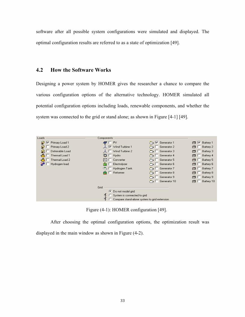
4.2 How the Software Works

Designing a power system by HOMER gives the researcher a chance to compare the

various configuration options of the alternative technology. HOMER simulated all

potential configuration options including loads, renewable components, and whether the

system was connected to the grid or stand alone; as shown in Figure [4-1] [49].

Figure (4-1): HOMER configuration [49].

After choosing the optimal configuration options, the optimization result was

displayed in the main window as shown in Figure (4-2).

Figure (4-2): HOMER main window.

The information regarding the alternative power in question was entered into

HOMER by the user.

4.2.1 The Load

The electric demand and type was entered by entering or uploading the load file.

HOMER also needs information regarding the electricity load depicted per hour for one

full year (this is a total of 8,760 values) [49].

After entering the load information, the information is displayed in both diagram

and table formats. The load data collected from a sample factory in Saudi Arabia was

used as a base for calculating potential results. The solar radiation and temperature of the

region was also obtained for the calculations [49]. Both cost and features of the PV

systems were as shown in Appendix (A).

4.2.2 System Components

Each component of the system in the simulation needs to have a corresponding cost,

range, and lifetime. The costs of the component was divided into three parts, capital cost,

replacement cost, and operating and maintenance cost as shown in Figure (4-3). In

addition to the aforementioned costs, the size of the generator being considered is also

necessary for accurate calculations and simulation [49].

Figure (4-3): The components cost and range [49].

4.2.3 Grid Input

If the system is grid connected, the required data includes the tariff and FiT set by the

utility to buy and sell electricity. The price of electricity in Saudi Arabia depends on the

sector, time of day consumption and time of year consumption Figure (4-4).

Figure (4-4): HOMER grid window.

HOMER simulates these options by using the scheduled rate entered by the user.

4.2.4 Solar Resource Input

The inputs described the availability of solar radiation for each hour of the year. These

values are either attained by an uploaded file of a calculation option available in HOMER

to synthesize hourly data and or average monthly values as shown in Figure (4-5) [49].

Figure (4-5): HOMER solar resource window.

4.2.5 Temperature Input

Temperature has a direct effect on the efficiency of PV panels. Inputting the temperature

is a crucial step in calculating the amount of potential power produced by the PV array at

any given time during the year. Therefore, an hourly average temperature needs to be

entered (this also comes to a total of 8,760 values) as show in Figure (4-6) [49].

Figure (4-6): HOMER temperature window.

4.2.6 The Economic Input

Figure (4-7) illustrates the economic information that HOMER needs for the simulation.

In order to calculate the economic input, the annual real interest rate and project lifetime

need to be entered by the researcher [49].

Figure (4-7): HOMER economic window.

4.2.5 Constraints

Constraints are the conditions and configuration limits, which the HOMER software

system must satisfy. Any values that do not meet the required conditions will not appear

in the results Figure (4-8).

Figure (4-8): HOMER constraints window.

4.2.6 Simulation and Results

HOMER uses the combination of values entered in the various component inputs to

simulate the power system. Any results that do not meet the load demands are labeled

inefficient or infeasible and are then disregarded by HOMER [49].

A list of system configurations that HOMER has deemed feasible is labeled

optimization results and is displayed in a table as shown in Figure (4-9). Optimization

results are listed in order of cost effectiveness. Cost effectiveness is calculated by the net

present cost which is labeled "Total NPC" in the results Table [49].

Figure (4-9): HOMER results window.

4.2.6.1 The Optimization Result

Optimization results can also be filtered to display only the most cost effective

configuration of each system. This is simply done by choosing the categorized

optimization option in HOMER Figure (4-10) [49].

Figure (4-10): HOMER optimization results.

All information regarding the economic or technical details of the simulated

configuration systems (example: cash flow, cost summary, and electrical output) are

displayed in simulation results windows. Hourly performance, and performance of each

component (example: the PV value, grid converter, etc.) are also displayed in the

simulation results window [49].

HOMER was used to simulate the optimal results with considerations of cost

effectiveness and a potential sellback revenue [49].

4.3 Input Data

4.3.1 The Factory Load

The following is the input data used in HOMER. The factory load was obtained from the

electricity bills of a sample factory in Saudi Arabia. The load is presented per month over

the course of year as shown in Table (4-1).

Table (4-1): The monthly factory load. Month KWh/month January 28,001.40 February 30,800.00 March 44,000.00 April 74,000.00 May 103,600.00 June 123,200.00 July 123,200.00

August 135,200.00 September 123,200.00

October 44,000.00 November 42,400.00 December 32,800.00

The monthly load data was analyzed and converted to a daily and hourly load.

The typical operating hours for most factories in Saudi Arabia is from 8:00am to 5:00pm

for five days a week with two days off. During working hours, it was assumed that the

factory used the highest load with only a minimum load used during the evenings and

nights.

The load was assumed to be 90% during operating hours and 10% during the

evenings and nights in the winter seasons. During the summer season, the load was

assumed to be 80% during the operating hours and 20% during the evenings and nights.

Figure (4-10) shows an example of the daily and monthly load for the factory.

Figure (4-11): The factory load.

Since the HOMER program needs the hourly data entries over the course of a

year, this required 7,860 different entries [49]. Figure (4-12) shows the load information

after being entered in HOMER.

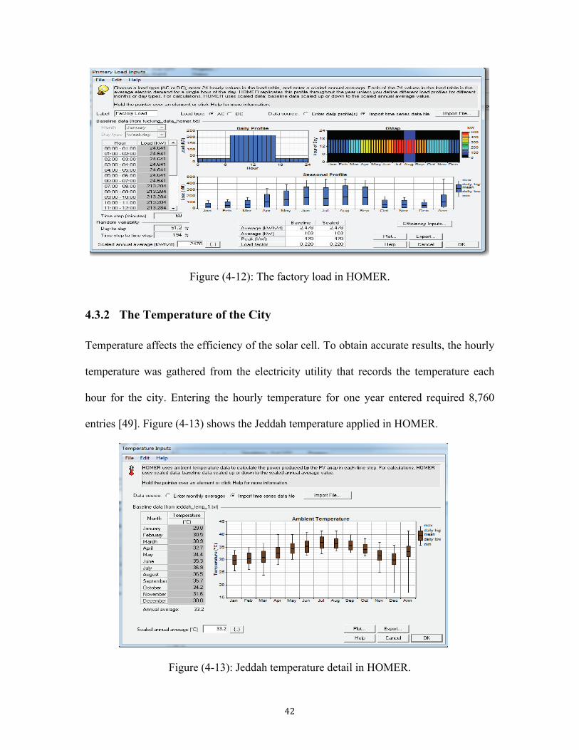
Figure (4-12): The factory load in HOMER.

4.3.2 The Temperature of the City

Temperature affects the efficiency of the solar cell. To obtain accurate results, the hourly

temperature was gathered from the electricity utility that records the temperature each

hour for the city. Entering the hourly temperature for one year entered required 8,760

entries [49]. Figure (4-13) shows the Jeddah temperature applied in HOMER.

Figure (4-13): Jeddah temperature detail in HOMER.

4.3.3 Solar Equipment Specifications

1- The PV kit: The kit price includes all the equipment needed to connect to the panel.

The extra costs such as costs for installation, shipping and engineering was added to the

price before the cost was calculated per KW. The replacement price needed at the end of

the kit’s life cycle is assumed to be the same as the starting price. The PV panel does not

require any maintenance after installation.

Table (4-2): The PV kit price.

PV (3

00W

)

Solar Kit type 639 Charger price 210

Price 429 Installation (10%) 43

Shipping & Eng. (20%) 86 Total for 300w 558

1KW price 1,859 O&M (0%) 0.00

Replacement 1859 Lifetime 25

Module cost /w 1.859043333

For the panel specification used in the data sheet in appendix B, the price was

obtained from the internet, as shown in appendix A. The price used may be decreased if

more than one kit is ordered. In addition, increasing the size of the PV system will

decrease the price therefore, the price of the kit was assumed at its highest possible price.

The size was entered with a wide range to give HOMER a chance to find the

optimal size for the system. All of the aforementioned specifications for the panel were

entered in HOMER such as the costs, the size, the properties and taking into

consideration the effect of the temperature Figure (4-14).

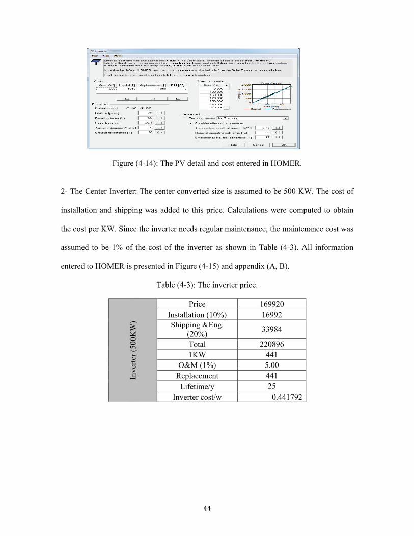
Figure (4-14): The PV detail and cost entered in HOMER.

2- The Center Inverter: The center converted size is assumed to be 500 KW. The cost of

installation and shipping was added to this price. Calculations were computed to obtain

the cost per KW. Since the inverter needs regular maintenance, the maintenance cost was

assumed to be 1% of the cost of the inverter as shown in Table (4-3). All information

entered to HOMER is presented in Figure (4-15) and appendix (A, B).

Table (4-3): The inverter price.

Inve

rter (

500K

W)

Price 169920 Installation (10%) 16992 Shipping &Eng.

(20%) 33984

Total 220896 1KW 441

O&M (1%) 5.00 Replacement 441 Lifetime/y 25

Inverter cost/w 0.441792

Figure (4-15): The PV detail and cost entered in HOMER.

4.3.4 The Grid Information

The rate used is the current price of electricity in Saudi Arabia. The exact cost was used

because the Saudi Arabia electricity company has different electricity tariffs depending

on the sector, season, and time. The Saudi Arabian tariff for the industrial sector was

obtained from the electricity utility then converted to dollars and entered intoHOMER

[32].

Up to now there has been no regulation for the FiT in Saudi Arabia. For this study

therefore two scenarios will be assumed. In the first scenario the sellback price will be

equal to the FiT price of the utility. Figure (4-16) shows the rate schedule for the tariff

and FiT used in the first scenario.

Figure (4-16): First scenario grid rate schedule.

In the second scenario, the sellback price is assumed to be the highest tariff price.

The reason for this assumption is that the PV system will be providing power during peak

hours; therefore, it is fair to assume a peak hour price. Figure (4-17) shows the rate

schedule for the second scenario.

Figure (4-17): Second scenario grid rate schedule.

4.3.5 Solar Resource

The solar radiation was generated automatically by HOMER. This can be done by

inserting the required coordinates of the selected area. Figure (4-18) shows the daily

radiation and clearness index for every month of the year generated by HOMER. The

maximum radiation is about 5.6 kWh/m3/d, which is enough to generate the required

power for the area.

Figure (4-18): Solar radiation and clearness index.

4.3.6 Economic Entries

The most important economic factors for HOMER are the real interest rate and the

project lifetime. For the real interest rate (discount rate) in Saudi Arabia 2% was added.

The normal project lifetime for any PV system is between 25-30 years. A 25-year

lifetime was chosen and was added to HOMER Figure (4-19).

Figure (4-19): The economic information.

4.3.7 Constraints

HOMER was forced to follow the assumption that chose the fraction covered by the PV

system. The fraction chosen is shown in Figure (4-20).

Figure (4-20): The fraction covered by PV system.

All data was entered into HOMER for simulation. Figure (4-21) shows the final system

configuration after all the data needed for the simulation was entered.

Figure (4-21): System configuration.

4.6 The Economic Calculation

4.6.1 Introduction

After completing the technical requirements and design of a PV system, an economic

analysis that breaks down the costs and benefits of the system is necessary [50].

The costs of a PV system are broken down into various sub-costs. These sub-costs

include the cost required to acquire the system, initial operating costs, maintenance costs

and replacement costs [51].

At the end of the life of a system, a projected salvage and or decommissioning

cost is needed. Life cycle costing is a method often used to project costs of the PV

system. Life cycle costing refers to an evaluation of all purchase choices. [51]. In order to

evaluate this, the Net Present Value (NPV), payback period, and Internal Rate of Return

(IRR) methods are used [52].

4.6.2 Economic Factors

Before we start there are some factors that need to be defined:

4.6.2.1 The Discount Rate (i)

The discount rate (also referred to as the opportunity cost) refers to the value the owner

contributes towards the capital invested in the system [50]. This factor is determined by

the bank. When an investment is made on a renewable energy system, the rate is referred

to as the discount rate. In other words, the amount of interest determined by the bank is

an amount that can be earned on the principal saved. Therefore, the principal may

increase yearly if the account is determined to have a positive rate. This can be

problematic if the amount determined is greater than the rate of inflation [51].

The real challenge in investing money is to invest at a discount rate that is greater

than the inflation rate [51].

4.6.2.2 The Capital Recovery Factor (CRF)

“A capital recovery factor is the ratio of a constant annuity to the present value of

receiving that annuity for a given length of time” [50].

The CRF can be calculated by:

CRF = m(1+m)n(1+m)n −1

(4-1)

[50]

m in the aforementioned equation is equal to the discount rate.

4.6.3 Net Present Value and Future Worth

In the equation below, P refers to a sum received at a current time and has a determined

present value. F refers to a sum spent in the future and has a determined future value.

Therefore, if P is invested considering the discount rate (i), the future value is calculated

using the following equation [50]:

F = P(1+ i)n (4-2)

[50]

For the inverse relation, a present value of a future sum is calculated using the

following equation:

P = F(1+ i)−n (4-3)

[50]

4.6.4 Life Cycle Cost (LCC)

4.6.2.1 Definition

The life cycle cost (LCC) analysis is an analysis used to asses all costs pertaining to the

life of the project. This is done with consideration for all costs (capital investment costs,

purchasing costs, installations costs, operating costs, maintenance costs, and future

salvage costs) [53].

4.6.2.2 Life-Cycle Cost Formula

To calculate and find the total LCC of a project, a sum of all costs is generated then a

present cash value (example: resale worth) is deducted.

LCC = Initial cost + electricity cost + O& M cost + replacement cost – salvage (4-4)

[54]

1- Initial cost: is the price of all components in the PV system such as the PV panel,

inverter and cables [54].

In addition, there are other parameters that will be added to the initial cost

including installation cost, shipping costs and engineering costs.

Initial cost = equipment cost + shipping cost +Eng. Cost + installation cost (4-5)

2- Maintenance cost: System maintenance is a recurring cost over the project lifetime.

This includes all equipment maintenance, site maintenance, and all required system

supervision. PV systems require very little maintenance.

P = aunnual.main. * [(1+ i)n −1]

[i(1+ i)n ] (4-6)

[50]

3- Replacement cost:

P = aunnual.rep* [(1+ i)n −1]

[i(1+ i)n ] (4-7)

[50]

4- Electricity cost: “The monetary value of all electricity used over the total life cycle of

the system” [55].

5 -Salvage cost: The salvage cost of a system refers to any remaining value at the end of

the life cycle or at the time of replacement [53].

4.6.2.3 Annualized life cycle cost (ALCC):

The levelized energy cost (LEC) is often generated by energy providers such as utilities.

This number provides a unit cost of electricity in $/kWh that remains invariable. This

method uses the present worth of a cost and the capital recovery factor divided by the

annual energy produced by the system, to generate an annual cost of electricity [50].

(4-8)

[50]

NPWC refers to the present value .The term E refers to the annual energy in

kilowatts per hour that is generated by the system.

LEC = (NPWc )(CRF)E

4.6.5 Internal Rate of Return (IRR)

An internal rate of return (IRR) refers to a calculation method where the NPV equals

zero. The discount rate is then assumed to be equal to the IRR. This assumption is often

recommended when comparing projects of equal survival and possible risks. The project

with the highest IRR is the optimal choice [56].

(4-9)

[50]

The assessment figure of IRR that satisfies the aforesaid equation is the

assessment that should be accepted.

4.6.6 Payback Period (PB)

One of the great advantages of PV systems is that they are able to function for a long

time. Solar panels are often guaranteed for 25 years and it is suggested that they will most

likely perform successfully beyond 25 years with the proper maintenance. Therefore, a

payback calculation needs to consider the savings that come with a solar system across a

25-year period. In addition, the parameters that effect the payback to make PV grid

connected system more efficient must also be studied [57].

In order to determine the payback period, the following steps were used:

Step 1: The initial yearly savings as a result of using a PV system are determined. This is

done by computing the output of the proposed system in kilowatt hours [57].

Step 2: Future increases in electrical costs were considered and included [57].

Step 3: The yearly savings were then multiplied by the future inflation rate [57].

0 = Ps(1+ IRR)nn=0

L

∑

Step 4: The aforementioned savings are then accumulated by year: This is done by

adding the prior year's savings (whether adjusted for inflation) to the current year savings

[57].

Step 5: The initial cost is then deducted from the potential accumulated savings. This will

initially generate a positive number for the initial cost. However, over time the savings

will surpass the initial cost. The point at which the savings surpass the initial cost is

referred to as the payback period [57].

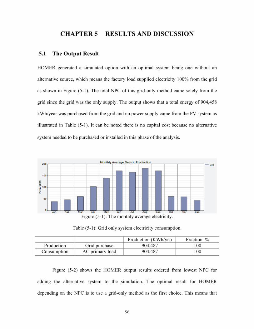
CHAPTER 5 RESULTS AND DISCUSSION

5.1 The Output Result

HOMER generated a simulated option with an optimal system being one without an

alternative source, which means the factory load supplied electricity 100% from the grid

as shown in Figure (5-1). The total NPC of this grid-only method came solely from the

grid since the grid was the only supply. The output shows that a total energy of 904,458

kWh/year was purchased from the grid and no power supply came from the PV system as

illustrated in Table (5-1). It can be noted there is no capital cost because no alternative

system needed to be purchased or installed in this phase of the analysis.

Figure (5-1): The monthly average electricity.

Table (5-1): Grid only system electricity consumption.

Production (KWh/yr.) Fraction % Production Grid purchase 904,487 100

Consumption AC primary load 904,487 100

Figure (5-2) shows the HOMER output results ordered from lowest NPC for

adding the alternative system to the simulation. The optimal result for HOMER

depending on the NPC is to use a grid-only method as the first choice. This means that

any alternative system will not be considered an optimal solution. The reason for this is

the grid-only system is assumed to carry no capital or maintenance cost.

It can then be deduced that the most cost effective option is to use the supply from

the grid only system without a PV generator. This option has a total net present cost

(NPC) of $708,234 and the lowest cost of energy (COE) of $0.04/kWh. This option also

results in an operating cost of $36,276/year. The operating cost was generated by

multiplying the total energy purchased by the purchase prices. The initial capital cost in

this case is zero due to the lack of a PV generator and inverter.

Figure (5-2): The overall results from HOMER.

For the optimal overall result HOMER gives only two systems, as shown in

Figure (5-3).

Figure (5-3): The optimization system results.

From Figure (5-3) there is only one optimal system with a PV system. This

system has a PV fraction of 18% with a grid fraction of 82%.

For the optimal alternative system, the PV system and inverter size are 100 KW

as shown in Table (5-2) with a capital cost of $185,900and $44,200 for the PV kit and

inverter respectively. For the O%M the PV cost was assumed to be zero while the

inverter is $9,762.

Table (5-2): The PV system size and cost.

Component Size (KW) Capital cost ($) O&M ($) Total ($) PV Kit 100 185,900 0 185,900 Inverter 100 44,200 9,762 53,962

The alternative system with 18% fraction produces 170,155 KWh per year. On the

other hand, the system purchases 762,458 KWh per year from the grid.

The system was sold back to the grid at 23,0537 KWh/yr, which is only 2%

fraction on the total power consumption while the 98% fraction consumed by the load.

The excess electricity is zero as shown in Table (5-3).

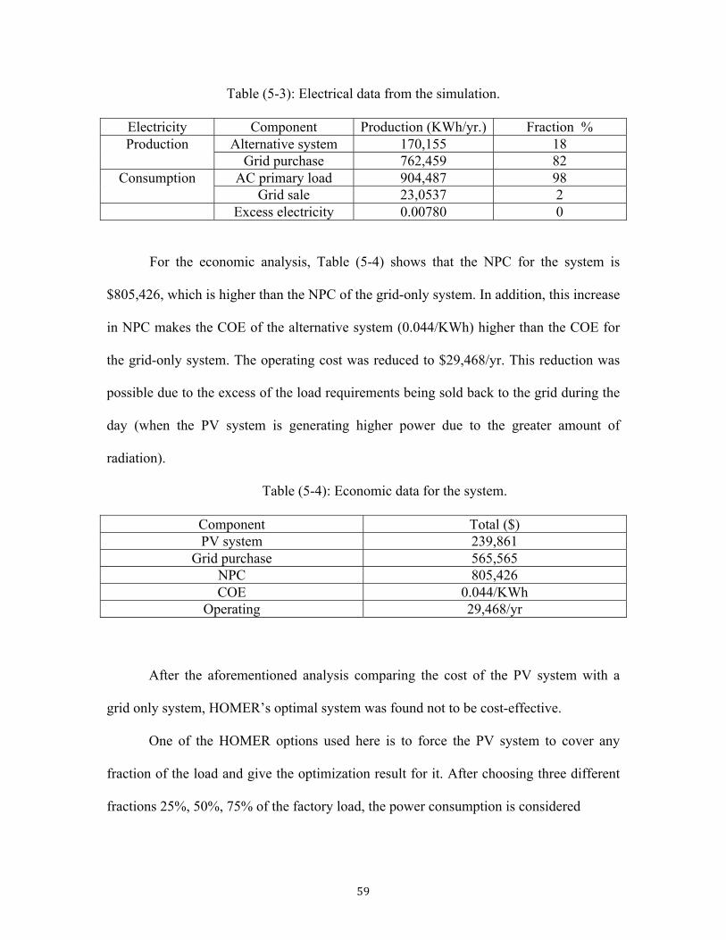
Table (5-3): Electrical data from the simulation.

Electricity Component Production (KWh/yr.) Fraction % Production Alternative system 170,155 18

Grid purchase 762,459 82 Consumption AC primary load 904,487 98

Grid sale 23,0537 2 Excess electricity 0.00780 0

For the economic analysis, Table (5-4) shows that the NPC for the system is

$805,426, which is higher than the NPC of the grid-only system. In addition, this increase

in NPC makes the COE of the alternative system (0.044/KWh) higher than the COE for

the grid-only system. The operating cost was reduced to $29,468/yr. This reduction was

possible due to the excess of the load requirements being sold back to the grid during the

day (when the PV system is generating higher power due to the greater amount of

radiation).

Table (5-4): Economic data for the system.

Component Total ($) PV system 239,861

Grid purchase 565,565 NPC 805,426 COE 0.044/KWh

Operating 29,468/yr

After the aforementioned analysis comparing the cost of the PV system with a

grid only system, HOMER’s optimal system was found not to be cost-effective.

One of the HOMER options used here is to force the PV system to cover any

fraction of the load and give the optimization result for it. After choosing three different

fractions 25%, 50%, 75% of the factory load, the power consumption is considered

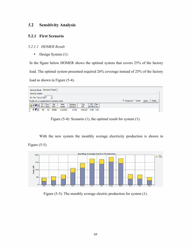
5.2 Sensitivity Analysis

5.2.1 First Scenario

5.2.1.1 HOMER Result

• Design System (1):

In the figure below HOMER shows the optimal system that covers 25% of the factory

load. The optimal system presented required 26% coverage instead of 25% of the factory

load as shown in Figure (5-4).

Figure (5-4): Scenario (1), the optimal result for system (1).

With the new system the monthly average electricity production is shown in

Figure (5-5).

Figure (5-5): The monthly average electric production for system (1).

The new PV system configuration shown in Table (5-5) shows that the new

bigger PV panel size obtained for the optimal system is the same size of the inverter. The

PV size is 150 KW with a capital cost of $ 278,850 while the maintenance costs are equal

to zero. The inverter cost with the regular maintenance equals $53,962.

Table (5-5): Scenario (1) system size and cost for system (1).


Table (5-6) shows the details of the electrical production and consumption. The

26% of the factory load supplied by the alternative system produced 255,232KWh/yr

while the rest of the load (74%) supplied by the grid produced 705,404KWh/yr. In this

option, the system still gets most of the power from the grid. In addition the system

sellback is 5.902 KWh/yr to the grid while the excess electricity is less than 1%.

Table (5-6): Scenario (1) Electrical detail for system (1).

Production (KWh/yr.) Fraction % Production Alternative system 255,232 26


Grid sale 5.902 5 Excess electricity 42,797 0.6

The cost of the alternative system is $332,811. The NPC, COE and operating cost

of the new system are 853697$, 0.046/KWh and 27,180/yr respectively. Most of the

power is still purchased from the grid ($520,886) Table (5-7).

Table (5-7): Scenario (1) Economic analysis for system (1).


Grid purchase 520,886 NPC 853,697 COE 0.046 /KWh

Operating 27,180 /yr.

• Design System (2): In Figure (5-6) below HOMER shows the optimal system for a new fraction. The PV

system size increased to 330 KW while the inverter size increased to 250 KW.


The new system covers 50% of the total factory load. The optimal system is to

cover 52% instated of 50% of the factory load. Figure (5-7) shows the monthly average

electrical production with system 2.

Figure (5-7): The monthly average of electric production for system (2).

The new PV system configuration shown in Table (5-8) shows that the new larger

PV panel size costs $613,470 while the new inverter total costs $134,904.

Table (5-8): Scenario 1 system size and cost for system (2).

Component Size (KW) Capital cost ($) O&M ($) Total ($) PV Kit 330 613,470 0 613,470 Inverter 250 110,500 24,404 134904

Table (5-9) shows the detail of the electrical production and consumption. The

alternative system supplied 52% of the factory load and produced 561,513KWh/yr while

the rest of the load (48%) was supplied by the grid and produced 519,993KWh/yr. The

system is starting to get a higher amount of power from the PV system than from the grid.

In addition, the system sell-back was 158,33 KWh/yr to the grid with excess electricity of

less than 1%.

Table (5-9): Scenario (1) Electrical detail for system (3).

Electricity Component Production (KWh/yr.) Fraction % Load

Production Alternative system 561,513 52 Grid purchase 519,993 48

Consumption AC primary load 904,487 85 Grid sale 158,33 15

Excess electricity 1,878 0.17

The cost of the alternative system is $748,374. The NPC, COE and operating cost

of the new system are 1,036,186$, 0.05/KWh and 15,992/yr respectively. The grid

purchase cost is $287,812, as shown in Table (5-10).

Table (5-10): Scenario (1) Economic data for the system (2).


Grid purchase 287,812 NPC 1,036,186 COE 0.050 /KWh


• Design System (3): Covering 75 % of the Total Load

HOMER shows the optimal system for a new fraction in Figure (5-8). The new PV

system size is 600 KW while the inverter size is 480KW. The total net present cost is

$1,327,560


Figure (5-9): The monthly average electrical production.

System 3 covers 75% of the factory load. The optimal system is to cover 76%

instead of 75% of the factory load. The Figure (5-9) shows the monthly average

electrical production with the new system.

The new PV system configuration shown in Table (5-11) shows that the new

bigger PV panel size cost $1,115,400 while the new inverter total cost $259,016.

Table (5-11): Scenario (1) size and cost for system (3).

Component Size (KW) Capital cost ($) O&M ($) Total ($) PV Kit 600 1,115,400 0 1,115,400 Inverter 480 222,160 46,856 259.016

Table (5-12) shows the detail of the electrical production and consumption. The

76% of the factory load supplied by the alternative system produced 1,020,929 KWh/yr

while the rest of the load (24%) supplied by the grid produced 329,716 KWh/yr. The new

system gets most of the power from the PV system rather than from the grid. In addition,

the system sellback was 414,655 KWh/yr to the grid while the excess electricity is still

less than 1%.

Table (5-12): Scenario (1), Economic analysis for system (3).


Production Alternative system 1,020,929 76 Grid purchase 329,716 24


Excess electricity 933 0.07

Table (5-13) shows the cost of the alternative system is $1,374,416, which makes

it the highest cost variable. The NPC and the COE of the new system are 1,316,460$,

0.051/KWh respectively. The grid purchase and the operating cost in this system is a

negative value that means the system produced more power than the required amount to

cover the load and sell it to the grid.

Table (5-13): Scenario1, Economic data for the system (3).

Component Total ($) PV system 1374416

Grid purchase -57,956 NPC 1,316,460 COE 0.051

Operating -563/yr

The summary table for the results from HOMER for the first scenario is shown in

Table (5-14).

Table (5-14): Scenario (1), the summary table for scenario (1).

Load cover by PV 25% 50% 75% Homer % 26% 52% 76% PV size / inverter size 150/100 330/250 600/480 COE 0.046 0.050 0.051 NPC 853,697.00 1,036,186.00 1,316,460.00

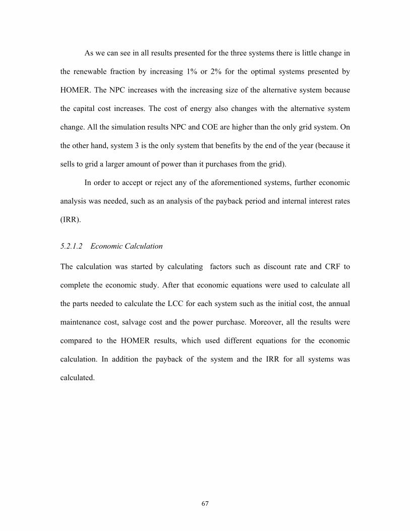
As we can see in all results presented for the three systems there is little change in

the renewable fraction by increasing 1% or 2% for the optimal systems presented by

HOMER. The NPC increases with the increasing size of the alternative system because

the capital cost increases. The cost of energy also changes with the alternative system

change. All the simulation results NPC and COE are higher than the only grid system. On

the other hand, system 3 is the only system that benefits by the end of the year (because it

sells to grid a larger amount of power than it purchases from the grid).

In order to accept or reject any of the aforementioned systems, further economic

analysis was needed, such as an analysis of the payback period and internal interest rates

(IRR).

5.2.1.2 Economic Calculation

The calculation was started by calculating factors such as discount rate and CRF to

complete the economic study. After that economic equations were used to calculate all

the parts needed to calculate the LCC for each system such as the initial cost, the annual

maintenance cost, salvage cost and the power purchase. Moreover, all the results were

compared to the HOMER results, which used different equations for the economic

calculation. In addition the payback of the system and the IRR for all systems was

calculated.

Table (5-15): Scenario (1), economic calculation.

Discount rate 0.02 Years 25 CRF 0.051220438 System1 System2 System3

System size KW 150 330 600 PV

Price 278,850.00 613,470.00 1,115,400.00 Annual main 0.00 0 0 LCC.main 0.00 0 0 Life time 25.00 25 25

Total price 278850.00 613,470.00 1,115,400.00 Price /w 0.049 0.054 0.052 Inverter 100 250 480

Price $44,200.00 $110,500.00 $212,160.00 Annual main. 500.00 1250.00 2400.00 LCC main. 9,761.00 24,404.00 46,856.00 Life time 25.00 25.00 25.00

Total price 44200.00 110500.00 212160.00 Price /w 0.42 0.42 0.42

System price Capital cost 332,811.00 748,374.00 1,374,416.00

Grid purchase 520,886.00 287,812.00 -$57,956.00 Total cost 853,697.00 1,036,186.00 1,316,460.00

Total power product 960,637.00 1,081,506.00 1,350,646.00 COE 0.046 0.05 0.050

Salvage cost 66,562.20 149,674.80 274,883.20

From Table (5-15) we see similar results as from HOMER software, such as total

system cost and the COE. To calculate the payback, the total yearly income gathered

from selling electricity to the grid with the various seasonal and weekday changes of

tariff were taken into consideration and illustrated in Table (5-16).

Table (5-16): Calculation the total price of sold power.

Total price of power sold PV system size Period Price c/kw Sys1 Sys 2 Sys 3 12h 0.032 $31,587.00 $109,686.00 $302,386.00 15h 0.04 $4192 $16723 $35983 10h 0.027 $108 $3048 $12766 26h 0.069 $6910 $28922 $63520 Total price $1,658.17 $6,256.79 $15,843.23

The electricity rate annual inflation was also considered, this was calculated to be

(i) to be equal to the inflation in Saudi Arabia = 4% [58].

5.2.1.3 Payback for scenario (1) systems

1- The payback for system (1):

Table (5-17): Scenario (1), the payback for system (1).

System 1 Revenues &expenses Year 0 Year 1 Year 2 Year 24 Year 79 Initial cost &salvage -$853,697.00 33,281.10

Power sales 1,658 1,724 4,087 35,337 Cumulative elec. sales 1,658 3,383 64,806 877,307

Simple payback -852039 -850314 -788891.40 23610.42

From Table (5-17) system (1) will take 79 years (which is more than the project life).

This made the system not cost-effective and unacceptable. Since the system was not cost

effective and the payback was more than the lifespan of the IRR the resulting negative

calculation is not acceptable.

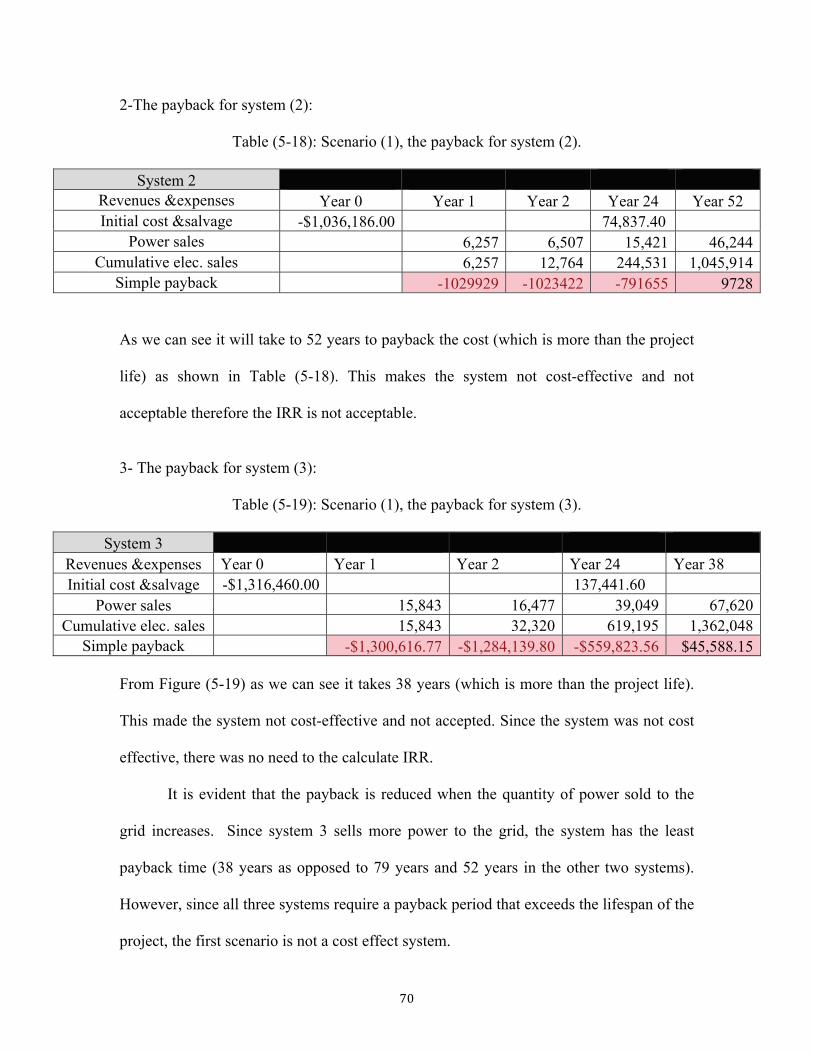
2-The payback for system (2):


System 2 Revenues &expenses Year 0 Year 1 Year 2 Year 24 Year 52 Initial cost &salvage -$1,036,186.00 74,837.40

Power sales 6,257 6,507 15,421 46,244 Cumulative elec. sales 6,257 12,764 244,531 1,045,914

Simple payback -1029929 -1023422 -791655 9728

As we can see it will take to 52 years to payback the cost (which is more than the project

life) as shown in Table (5-18). This makes the system not cost-effective and not

acceptable therefore the IRR is not acceptable.

3- The payback for system (3):



Power sales 15,843 16,477 39,049 67,620 Cumulative elec. sales 15,843 32,320 619,195 1,362,048

Simple payback -$1,300,616.77 -$1,284,139.80 -$559,823.56 $45,588.15

From Figure (5-19) as we can see it takes 38 years (which is more than the project life).

This made the system not cost-effective and not accepted. Since the system was not cost

effective, there was no need to the calculate IRR.

It is evident that the payback is reduced when the quantity of power sold to the

grid increases. Since system 3 sells more power to the grid, the system has the least

payback time (38 years as opposed to 79 years and 52 years in the other two systems).

However, since all three systems require a payback period that exceeds the lifespan of the

project, the first scenario is not a cost effect system.

5.2.1.4 Conclusions for Scenario (1)

Comparing all systems to the grid-only system was not cost effective. All the systems

have a higher NPC because of the initial cost for the PV system and the fact that the grid

system is the only system with a lower COE. In addition, the assumed sellback price is

not acceptable because even the system selling the most power to the grid was still

economically not acceptable.

5.2.2 Second Scenario

In the second scenario we have changed the feed-in tariff to find a cost effective system,

assuming the power utility will pay for electricity at a higher price (0.069c/kw) than they

sell the power to the industrial sector.

5.2.2.1 HOMER Result


PV system size and cost:

The PV system configuration shown in Table (5-20) shows the same size of the inverter.

The PV size is 150 KW with a capital cost of $278,850 while the maintenance is equal to

zero. The inverter cost with regular maintenance is equal to $53,962

Table (5-20): Scenario (2) system (1) size and cost.


In this scenario’s first system, 26% of the factory load is supplied by the

alternative system while the rest of the load (74%) is supplied by the grid, illustrated in

Table (5-21). In addition, the system sells 5.9 KWh/yr to the grid while the excess

electricity is less than 1%

Table (5-21): Scenario (2) Electrical data for system (1).

Production (KWh/yr.) Fraction % Production Alternative system 255,232 26


Grid sale 5.902 5 Excess electricity 42,797 0.6

Table (5-22): Scenario 2 Economic data for system (1).


Grid purchase 495,606 NPC 828,417 COE 0.045 /KWh


From Table (5-22) the only change with the new feed-in tariff is the grid purchase

because the price for sellback change makes the grid purchase decrease. This makes the

NPC of the system decrease, thus also making the COE decrease. Finally this shows the

sellback is effective economically.


From Tables (5-23, 24) there is no change in the size and the cost of the optimal system.

Also there is no change in the electrical consumption.

Table (5-23): Scenario (2) system (2) size and cost.

Component Size (KW) Capital cost ($) O&M ($) Total ($)

PV Kit 330 613,470 0 613,470 Inverter 250 110,500 24,404 134904

Table (5-24): Scenario (2) Electrical data for system (2).


Production Alternative system 561,513 52 Grid purchase 519,993 48



The change in the new scenario took place in the economic analysis portion. The

grid purchase was reduced from $287,812 to $196,592. Thus the NPC also decreased,

which affected the COE. The COE reduced from 0.05/KWh to 0.046/KWh, as shown in

Table (5-25).

Table (5-25): Scenario (2) Economic data for system (2).


Grid purchase 196,592 NPC 944,966 COE 0.046/KWh




For the biggest system fraction coverage of the load, the optimal system from

HOMER totally changed. The new system with a different size and cost was obtained, as

shown in Figure (5-10). In addition, the fraction also changed from 77% to 79% with a

2% increase from the system in the first scenario. The monthly average electricity

production for system3 is shown in Figure (5-11)

Figure (5-11): Scenario (2) the monthly average for system (3).

For system 3, the new size of the PV system is 650KW while the inverter size is

reduced to 460KW. The total cost for the PV kit is $1,208,350. The inverter cost and

maintenance cost $248,224 as shown in Table (5-26).

Table (5-26): Scenario (2), PV system size and cost for system (3).

Component Size (KW) Capital cost ($) O&M ($) Total ($) PV Kit 650 1,208,350 0 1,208,350 Inverter 460 203,320 44,904 248,224

Table (5-27) shows the details of the electrical production and consumption.

When 79% of the factory load was supplied by the alternative system, the system

produced 1,106,007 KWh/yr while the rest of the load (21%) supplied by the grid

produced 302,759 KWh/yr. The system can cover the load but the electricity needed to

operate during the evening and night still comes from the grid. In addition, the system

sellback fractions increased to 34% and sold 459,428 KWh/yr to the grid, while the

excess electricity was still less than 1%.

Table (5-27): Scenario (2), Electrical data for system (3).


Production Alternative system 1,106,007 79% Grid purchase 302,759 21



Table (5-28) shows the cost of the alternative system is $1,456,574, which makes

it the highest cost as the size changed. On the other hand, the NPC and the COE of the

new system are 1,036,136$, 0.04/KWh respectively. This is less than in system 3 in the

first scenario1, and is due to the fact that the grid purchase increased to $ -390,712 when

the feed-in tariff changed in the second scenario.

Table (5-28): Scenario (2), Economic results for system (3).

Component Total ($) PV system 1,456,574

Grid purchase -390,712 NPC 1,036,186 COE 0.040/KWh

Operating -17,712 /yr.

After running the simulation with the new FIT, the following results were

obtained as shown in Table (5-29):

Table (5-29): summary results for the second scenario.

PV % cover from the load 26% 52% 79% PV/ inverter size 150/100 330/250 650/460

NPC 828,417 944,966 1,065,862 COE 0.045 0.046 0.040

Electricity From the grid (kwh/year) 705,404 519,993 30,759 Electricity Sale to the grid (kwh/year) 42,797 158,397 459,428

5.2.2.2 Economic Calculation

The economic calculation for the three systems for the new scenario is shown in Table (5-30)

Table (5-30): The economic calculation for the second scenario.

Discount rate 0.02 Years 25 CRF 0.051220438 26% 52% 77%

System size KW 150 330 650

PV Price 278,850.00 613,470.00 1,208,350.00

Annual main 0.00 0 0 LCC.main 0.00 0 0 Life time 25.00 25 25

Total price 278850.00 613,470.00 1,208,350.00 Price /w 0.049 0.054 0.056

Inverter 100 250 460 Price $44,200.00 $110,500.00 $203,320.00

Annual Main. 500.00 1250.00 2300.00 LCC main. 9,761.00 24,404.00 44,903.00 Life time 25.00 25.00 25.00

Total price 44200.00 110500.00 203320.00 Price /w 0.42 0.42 0.42

System price Capital cost 332,811.00 748,374.00 1,456,573.00

Grid purchase 495,606 196,592.00 -$390,712.00 Total cost 828,417.00 944,966.00 1,065,861.00

COE 0.044 0.045 0.04 Salvage cost 83,202.8 187,093.50 364,143.25

Economic calculations showed similar results to the results simulated by

HOMER. To make the final decision on which system is the optimal system we need to

calculate the payback and IRR.

5.2.2.3 The payback for the second scenario

1- The payback for system (1)


System 1 Revenues &expenses Year 0 Year 1 Year 2 Year 24 Year 61 Initial cost &salvage -$828,417.00 33,281.10

Power sales 3,356 3,490 8,272 35,306 Cumulative elec.sales 3,356 6,847 131,170 834,058

Simple pay back -825061 -821570 -697246.83 5640.52



System 2

Revenues &expenses Year 0 Year 1 Year 2 Year 24 Year 38 Initial cost &salvage -$944,966.00 74,837.40

Power sales 11,488 11,947 28,314 49,030 Cumulative elec.

sales 11,488 23,435 448,963 987,587 Simple pay back -933478 -921531 -496003 42621


Table (5-33): Scenario (2), the payback for system (2)


Power sales 31,336 32,589 71,406 77,233 Cumulative elec.

sales 31,336 63,924 1,073,178 1,224,674 Simple payback -$1,034,526.48 -$1,001,937.54 $7,316.01 $190,147.32

The payback was reduced with the new FiT. In system 1 the payback was reduced

from 79 years to 61 years, as illustrated in Table (5-31). System 2 showed a payback

reduction from 52 years to 38 years, showin in Table (5-32). In Table (5-33) system 3

showed a payback reduction to 22 years, which is less than the lifetime of the system.

That makes system 3 the only cost effective system, as shown in Figure (5-12).

Figure (5-12): The payback for senior (2) for all systems.

After the payback results the last economic test for the system is the internal rate

of return (IRR). The IRR for the three systems with the new FiT is shown below:

Table (5-34): Scenario 2 the IRR for the systems.

Sell back Tariff = 0.069 System 1 System2 System3

Year 0 -$828,417.00 -$944,966.00 -$1,065,862.00 Year 1 $3,356.23 $11,487.53 $31,335.52 Year2 $3,490.48 $11,947.04 $32,588.94 Year3 $3,630.10 $12,424.92 $33,892.50 Year4 $3,775.30 $12,921.91 $35,248.20 Year5 $3,926.31 $13,438.79 $36,658.13 Year6 $4,083.37 $13,976.34 $38,124.45 Year7 $4,246.70 $14,535.40 $39,649.43 Year8 $4,416.57 $15,116.81 $41,235.41 Year9 $4,593.23 $15,721.48 $42,884.83 Year10 $4,776.96 $16,350.34 $44,600.22 Year11 $4,968.04 $17,004.36 $46,384.23 Year12 $5,166.76 $17,684.53 $48,239.60 Year13 $5,373.43 $18,391.91 $50,169.18 Year14 $5,588.37 $19,127.59 $52,175.95 Year15 $5,811.90 $19,892.69 $54,262.99 Year16 $6,044.38 $20,688.40 $56,433.50 Year17 $6,286.15 $21,515.94 $58,690.85 Year18 $6,537.60 $22,376.57 $61,038.48 Year19 $6,799.10 $23,271.64 $63,480.02 Year20 $7,071.07 $24,202.50 $66,019.22 Year21 $7,353.91 $25,170.60 $68,659.99 Year22 $7,648.07 $26,177.43 $71,406.39 Year23 $7,953.99 $27,224.52 $74,262.64 Year24 $8,272.15 $28,313.50 $77,233.15 Salvage

cost 83,202.75 $187,093.50 364,143.25

IRR -7% -2% 3%

For the IRR results, system 3 is the only system with an IRR larger than the

discount rate (2%). The other two systems have an IRR less than the discount rate, which

makes them unacceptable as illustrated in Table (5-34). The only acceptable system was

system 3.

As one of our goals was to reduce the power consumption from the utility, Figure

(5-13) describes the power purchase from the grid showing the relation between the

system size and the power purchased. System 3 reduced the power purchased from the

utility only in the summer, with the amount of power not exceeding 110,573KW in

August (the hottest month). That means using system 3 can reduce the power consumed

from the grid by 18.2% in the hottest month.

Figure (5-13): The power purchased from the grid.

Conclusions for scenario (2):

The simulation for the second scenario shows the same optimization results for the PV

system 1 and system 2 in the electricity consumption but with a change in the NPC and

the COE because of the new FiT. On the other hand, system 3 has a new size for the PV

and the inverter. System 3 has the best optimization results with the lowest COE equal to

the COE on the grid only, and a reduction in power purchased to 21% but with high NPC.

In addition, system 3 is the only system that has PB less than the lifetime of the system.

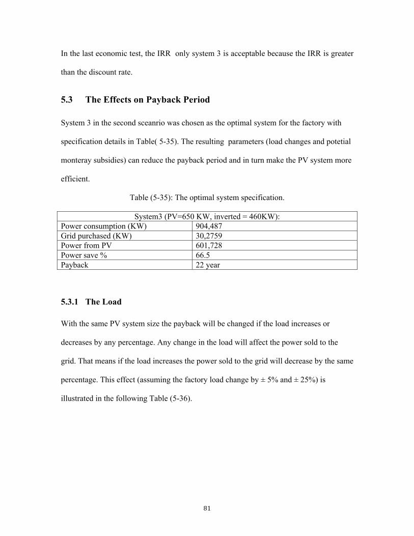
In the last economic test, the IRR only system 3 is acceptable because the IRR is greater

than the discount rate.

5.3 The Effects on Payback Period

System 3 in the second sceanrio was chosen as the optimal system for the factory with

specification details in Table( 5-35). The resulting parameters (load changes and potetial

monteray subsidies) can reduce the payback period and in turn make the PV system more

efficient.

Table (5-35): The optimal system specification.

System3 (PV=650 KW, inverted = 460KW): Power consumption (KW) 904,487 Grid purchased (KW) 30,2759 Power from PV 601,728 Power save % 66.5 Payback 22 year

5.3.1 The Load

With the same PV system size the payback will be changed if the load increases or

decreases by any percentage. Any change in the load will affect the power sold to the

grid. That means if the load increases the power sold to the grid will decrease by the same

percentage. This effect (assuming the factory load change by ± 5% and ± 25%) is

illustrated in the following Table (5-36).

Table (5-36): Load change.

Factory load +5% -5% +25% -25% Jan 28000 29400 26600 35000 21000 Feb 30800 32340 29260 38500 23100 Mar 44000 46200 41800 55000 33000 Apr 74000 77700 70300 92500 55500 May 103600 108780 98420 129500 77700 Jun 123200 129360 117040 154000 92400 Jul 123200 129360 117040 154000 92400 Aug 135200 141960 128440 169000 101400 Sep 123200 129360 117040 154000 92400 Oct 44000 46200 41800 55000 33000 Nov 42400 44520 40280 53000 31800 Dec 32800 34440 31160 41000 24600

Figure (5-14, 5-15) shows the change in the load in each month during the year

with the assumed percentage.

Figure (5-14): Load change by ± 5%.

Figure (5-15): Load change by ± 25%.

Changes to the factory load will affect the payback time. We assume that when

the load increases by 5% or 25% the power from the PV system that sells back to the grid

will decrease by the same percentage. Further, we assume that will also reduce the

revenue from using the PV connected grid will increase the power consumed from the

utility. Figures (5-16, 5-17) show the change in the payback time with different

percentages in the load change.

Figure (5-16): The payback for load change by 5%.

Figure (5-17): The payback for load change by 25%.

Table (5-37) shows the parameter change with load consumption change. First the

cost of the system will increase or decrease depending on the change in load. The

payback of the system also will change.

Table (5-37): The payback vs. load change.

Load change +5% -5% 25% -25%

Total cost 1,085,397.55 1,046,326.45 1,163,539.75 968,184.25 Power sales 29,768.75 32,902.30 23,501.64 39,169.40

Payback 22 20 23 18

Figure (5-18) shows the relationship between the changes in the load and the

payback time. The relationship shows that a reduction in the load consumption will

reduce the payback. Reducing the power consumption by 25% will reduce the payback to

18 years as opposed to 22 years with normal consumption.

Figure (5-18): Payback vs. load.

5.3.2 Subsidy by the Saudi Arabia Government:

Until now there is has been no government subsidy available for solar energy systems in

Saudi Arabia. If we assume that the government will potentially subsidize the initial cost

for a PV system by 10%, 15%, or 20 % the initial cost and total cost for the system is

shown in Table (5-38).

Table (5-38): The government subsidy table.

Subsidy 0% 10% 15% 20% Initial cost $ 1,411,670 1,411,670 1,411,670 1,411,670 Total subsidy $ 0 141,167 211,750.5 282,334 Total initial cost $ 1,411,670 1,270,503 1,199,919.5 1,129,336 Total system cost $ 1065861 924694 854110.5 783527

After we applied the different subsidy percentages to the system, we recalculated

the payback and IRR for each subsidy percentage. The first government subsidy

assumption is 10% therefore the initial cost will be $1,270,503 and the total cost will be

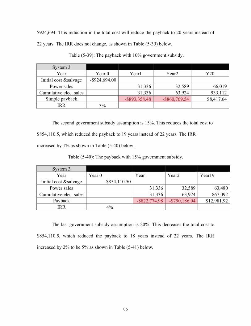
$924,694. This reduction in the total cost will reduce the payback to 20 years instead of

22 years. The IRR does not change, as shown in Table (5-39) below.

Table (5-39): The payback with 10% government subsidy.

System 3 Year Year 0 Year1 Year2 Y20

Initial cost &salvage -$924,694.00 Power sales 31,336 32,589 66,019

Cumulative elec. sales 31,336 63,924 933,112 Simple payback -$893,358.48 -$860,769.54 $8,417.64

IRR 3%

The second government subsidy assumption is 15%. This reduces the total cost to

$854,110.5, which reduced the payback to 19 years instead of 22 years. The IRR

increased by 1% as shown in Table (5-40) below.


System 3 Year Year 0 Year1 Year2 Year19


Cumulative elec. sales 31,336 63,924 867,092 Payback -$822,774.98 -$790,186.04 $12,981.92

IRR 4%

The last government subsidy assumption is 20%. This decreases the total cost to

$854,110.5, which reduced the payback to 18 years instead of 22 years. The IRR

increased by 2% to be 5% as shown in Table (5-41) below.


System 3 Year Year 0 Year1 Year2 Year18


Cumulative elec. sales 31,336 63,924 803,612 Payback -$752,191.48 -$719,602.54 $20,085.40

IRR 5%

Figure (5-19) shows that the government subsidy can reduce the payback and

make using the PV system connected grid more attractive to new consumers, especially

in the industrial sector, which can accept long run projects.

Figure (5-19): The payback vs. subsidy.

As the last point of this study, if we assume the Saudi government will subsidize

the PV connected grid in the industrial sector by 20% and the electricity utility applies

the new FiT, which was assumed in the second scenario the result would be a reduction

in load consumption by the factories by 25%. The optimal system we chose (system 3 in

the second scenario) will reduce costs to $685,850.25, illustrated in Table (5-42). Also

the payback decreased to 14 years, as shown in Figure (5-20).

Table (5-42): The final PV system cost.

The parameter Cost $ PV kit cost 1,208,350

Inverter cost 203,320 Total PV system cost 1,411,670

Total with subsidy 1,129,336 Maintenance 44,903 Capital cost 1,174,239

Grid purchase - 488,388.75 Total cost 685,850.25

Figure (5-20): The payback for the final system.

CHAPTER 6 CONCLUSIONS, RECOMMENDATIONS

AND FUTURE WORK

6.1 Conclusion

In conclusion this study used HOMER to simulate a potential application of a grid

connected PV system used to generate solar power in KSA. The daily energy

consumption used to simulate the system was gathered from a sample factory in the

industrial sector of the city of Jeddah. The average daily radiation and temperature was

used to assist in the simulation. The cost of the tariff for electricity was gathered from the

current utility in KSA. After using HOMER to simulate a potential optimal system two

scenarios were studied in depth.

The first scenario assumed FiT and examined three grid connected PV systems

used to generate solar power and sell the remaining power back to the grid. The cost of

the tariff used in the first scenario was the current tariff charged by the Saudi utility.

After an economic analysis this scenario was deemed not cost effective and therefore

disregarded.

The second scenario assumed that new FiT charged only at peak hours ( i.e the

highest tariff currently charged). This was assumed because the PV system would mainly

sell back power generated during peak hours. After an economic analysis this scenario

was deemed cost effective.

The payback period was studied to determine cost effectiveness. For each

scenario, three options were examined: 25% of the power generated from the PV system,

50% of the power generated from the PV system, and 75% generated from the PV

system. For both scenarios, option three, in which 75% of the power was generated from

the PV system, was chosen as the option with optimal payback. In the second scenario,

the combination of the high PV generation and increases in tariff for the sellback price

fostered the optimal overall solution. After examining the aforementioned options an

examination of a potential subsidy to supplement the cost of the PV system and a

potential load decrease improved the payback period even further.

6.2 Contribution

The purpose of this study is to examine the application of a PV grid-connected system as

an alternative source of electricity in industrial sector of Saudi Arabia.

This can also be stated as a question: “Does the PV system aid the industrial

sector in face of power cuts from the utility and can it be deemed economically

acceptable?” this gives rise to some sub-questions which this work answers:

• What is the feed-in tariff and how can it affect the PV system economically?

• How can the payback period be reduced and become more efficient?

• If the Saudi Arabian government gave attention and support to solar energy and

subsidizes electricity from the oil it will rollback with revenue.

6.3 Recommendations

1. Saudi Arabia should start applying regulations for use of solar energy, especially

the grid-connected system.

2. With the gulf electricity connection using the grid connected PV system, Saudi

Arabia will have the opportunity to sell more electricity and increase revenues.

3. In Saudi Arabia, using renewable energy in the second biggest electricity

consumption sector will reduce the production of CO2.

4. The Saudi Electricity Company should support the use of renewable energy in the

industrial sector. This support will benefit the company as it will reduce the

electricity overload, reduce the number of new stations built, and reduce the

heavy load on the stations which will in turn increase the lifespan of generators

and reduce the maintenance cost.

5. For factories, this will regularly cut the electricity consumption from the utility

and will also generate a second income revenue with long run projects.

6.4 Future Work

The focus of this thesis has been to find the optimal PV grid-connected system for the

example factory using a simulated economic study. However, future work based on this

study can be pursued in many directions. Some recommendations are listed below:

1. Investigate the reduction of power consumption of applying PV a grid-connected

system to all factories in the industrial city.

2. Examine the use of PV systems for electrical and thermal applications in the

industrial sector to show the reduced percentage of power consumption.

3. Study the benefit of using a PV grid-connected system in the industrial sector for

the electrical company suppliers to meet the growing city load without adding

new utility generation.

4. Combining an additional renewable energy source to the PV system supply to

further meet the growing electrical demands. For example wind power.

APPENDIX A: PV System Price

APPENDIX B: Technical Data for PV System Components

Bibliography

[1] Alyousef, Y., and Abu-ebid M., "Energy efficiency initiatives for Saudi Arabia on supply and demand sides," in Energy Efficiency - A Bridge to Low Carbon Economy, First ed., Zoran Morvaj, Ed. InTech, 2012, pp. 297-308. [2] Obaid, R.R., and Mufti, A.H., "Present state, challenges, and future of power generation in Saudi Arabia," in Energy 2030 Conference, USA, Nov,2008, pp. 1-6. [3] R. R. Obaid, "Reducing Peak Electricity Demand through 300MW Wind Farm North of Jeddah, Saudi Arabia," International Journal of Engineering and Technology, vol. 11, pp. 151-157, April, 2011. [4] Ministry of Economy and Planning, "Brief report on the ninth development plan (2010-2014)," Saudi Arabia, 2010. http://www.mep.gov.sa/themes/GoldenCarpet/index.jsp;jsessionid=3D9C02CB24CBC5E3504D0A99678CC2B6.alfa#1361213441247 [5] Alghamdi, J., "Power cuts hit industrial area in south Jeddah," Saudigazette, pp. 1p, Jun 16. 2009. http://www.saudigazette.com.sa/index.cfm?method=home.regcon&contentID=2009061640963 [6] Govinda, R. T., Lado, K., and Patrick, A. N., "A Review of Solar Energy: Markets, Economics and Policies", Oct, 2011. [7] Andreas, P., George, K, and Ioannis, H., "Parametric analysis for the installation of solar dish technologies in Mediterranean regions," Renewable and Sustainable Energy Reviews, vol. 14, pp. 2772-2783, Dec, 2010. [8] Tyagi, V. V., Kaushik, S. C., and Tyagi, S. K., "Advancement in solar photovoltaic/thermal (PV/T) hybrid collector technology," Renewable and Sustainable Energy Reviews, vol. 16, pp. 1383-1398, April, 2012. [9] Mekhilefa, S., Saidurb, R., and Safaria, A., "A review on solar energy use in industries,"Renewable and Sustainable Energy Reviews vol. 15, pp. 1777-1790, May, 2011. [10] Sater, B. L., "Solar cell," Physics Today, vol. 33, pp. 116-1p, Mar, 1980. [11] Paul, A. L., Electricity from Sunlight: An Introduction to Photovoltaics. UK: Chichester : Wiley, pp. 16, 2010. [12] Gilbert, M. M., Renewable and Efficient Electric Power Systems. NJ: Hoboken: John Wiley & Sons, pp. 445-512, 2004.

[13] Vinod, K. S., Antonio, C., and Giuseppe S., "Photovoltaic technology: Basic concepts, sizing of a stand alone photovoltaic system for domestic applications and preliminary economic analysis," Energy Conversion and Management, vol. 36, pp. 161-174, March, 1995. [14] Gilbert, M. M., Renewable and Efficient Electric Power Systems. NJ: Hoboken: John Wiley & Sons, pp. 31-32, 2004. [15] Paul, A. L., Electricity from Sunlight: An Introduction to Photovoltaics. UK: Chichester : Wiley, pp. 27-34, 2010. [16] Mitsubishi Electric, "Solar Power," pp. 1p, 2013 http://www.mitsubishielectric.com/bu/solar/faq/index.html [17] Ningbo best Solar, "Mono5” (r150)125s," Ningbo Best Solar Energy Technology Co., Ltd, pp. 1p, 2009. http://cnbestsolar.88582.net/High-efficiency-solar-cells/mono5”(r150)125s-_Mono5”(r150)125s-32.html [18] Shen Zhen Hui Xin Real Estate Co., Ltd, "Polycrystalline Silicon Solar Cell," pp. 1p, 2010. http://www.szshxzy.com/my/productshowen.asp?ID=2376 [19] Azursolar, "AZUR 2F: Light, Flexible But Still Strong," pp. 1p, 2013. http://com.azur-solar.de/products/azur-2f/ [20] Paul, A. L., Electricity from Sunlight: An Introduction to Photovoltaics. UK: Chichester: Wiley, pp. 103-142, 2010. [21] Vaughn Nelson, Introduction to Renewable Energy. FL: Boca Raton: CRC Press, pp. 115-119, 2011. [22] Access Solar, "stand-alone system," pp. 1p, 2013. http://accesssolar.lk/stand-alone-systems [23] Power House, "Solar PV (Photovoltaic) System," Power House Systems Inc, pp. 1p, 2013. http://solarpoweryourworld.com/faq/ [24] Fourth Coast, "Solar Photovoltaics," pp. 1p, 2011. http://fourthcoast.com/ [25] Almogren, S., and Veziroglu, T. N., "Solar-hydrogen energy system for Saudi Arabia," International Journal of Hydrogen Energy, vol. 29, pp. 1181-1190, Sep, 2004.

[26] A Hepbasli and Z Alsuhaibani, "A key review on present status and future directions of solar energy studies and applications in Saudi Arabia," Renewable and Sustainable Energy Reviews, vol. 15, pp. 5021-5050, Dec, 2011. [27] Pazheri F.R., Malik N.H., Al-Arainy A.A., Al-Ammar E.A., Imthias A. and Safoora O.K., "Smart grid can make saudi arabia megawatt exporter," in Power and Energy Engineering Conference (APPEEC), Asia-Pacific, 2011, pp. 1-4. [28] Wheeler, D., "A Solar Future for the World Bank in Southern Africa?" Global Development: Views from the Center, February 19, 2008. http://blogs.cgdev.org/globaldevelopment/2008/02/a-solar-future-for-the-world-b.php [29] Alyousef, Y., and Stevens, P., "The cost of domestic energy prices to Saudi Arabia," Energy Policy, vol. 39, pp. 6900-6905, Nov, 2011. [30] Aljarboua, Z., "The National Energy Strategy for Saudi Arabia," World Academy of Science, Engineering & Technology, vol. 57, pp. 501-510, Sep, 2009. [31] Embassy of Switzerland, "Saudi Arabia Major Business Sectors," OSEC Business Network Switzerland, Sep 11, 2011. http://www.osec.ch/de/sites/default/files/WZ_1109_E_Wirtschaftszweige-Saudi-Arabien.pdf [32] Saudi Electricity Company, "Tariff Rates," Online, 2008. http://www.se.com.sa/SEC/English/Menu/Customers/Consumption+bills/TarifAndTax.htm [33] Saudi Industrial Property Authority, "About MODON," Online, 2013. http://www.modon.gov.sa/English/AboutUs/Strategy/Pages/default.aspx [34] Kettani, M., "Photovoltaics in the Arab world," Solar Cells, vol. 6, pp. 234-249, August, 1982. [35] Sayigh, A. A. M., "Photovoltaic powered villages in Saudi Arabia," in Energy for Isolated Communities, IEE Colloquium on, 1988, pp. 2/1-4. [36] Salim, bbas A., and Eugenio, N. N., "A comprehensive report on the performance of the longest operating 350 kW concentrator photovoltaic power system," Solar Cells, vol. 29, pp. 1-24, June, 1990. [37]Alawaji, S., Smiai, M. S., Rafique, S. and Stafford, B., "PV-powered water pumping and desalination plant for remote areas in Saudi Arabia," Applied Energy, vol. 52, pp. 283-289, 1996.

[38] Alajlan, S.A. and Smiai, M.S., "Performance and development of PV - plant for water pumping and desalination for remote area in Saudi Arabia," Renewable Energy, vol. 8, pp. 441-446, Aug, 1996. [39] Al Harbi, Y., Eugenio, N.N. and Al Zahrani, S., "Photovoltaic-thermal solar energy experiment in Saudi Arabia," Renewable Energy, vol. 15, pp. 483-486, Dec, 1998. [40] Hasnain, S.M. and Alajlan, S., "Coupling of PV-powered R.O. brackish water desalination plant with solar stills," Renewable Energy, vol. 14, pp. 281-286, Aug, 1998. [41] Hasnain, S.M. and Alajlan, S., "Coupling of PV-powered R.O. brackish water desalination plant with solar stills," Desalination, vol. 116, pp. 57-64, Sep, 1998. [42] Elhadidy, M.A. and Shaahid, S.M., "Parametric study of hybrid (wind + solar + diesel) power generating systems," Renewable Energy, vol. 21, pp. 129-139, Oct, 2000. [43] Rehman, S., Shash, A. A. and Al-Amoudi, O. S. B., "Photovoltaic technology of electricity generation for desert camping," Int. J. of Global Energy Issues, vol. 26, pp. 322-340, 2006. [44] Shaahid, S.M. and El-Amin, I., "Techno-economic evaluation of off-grid hybrid photovoltaic–diesel–battery power systems for rural electrification in Saudi Arabia—A way forward for sustainable development," Renewable and Sustainable Energy Reviews, vol. 13, pp. 625-633, April, 2009. [45] Rehman S., Bader, M. A. and Al-Moallem, S. A., "Cost of solar energy generated using PV panels," Renewable and Sustainable Energy Reviews, vol. 11, pp. 1843-1857, Oct, 2007. [46] Shaahid, SM.and Elhadidy MA., "Economic analysis of hybrid photovoltaic–diesel–battery power systems for residential loads in hot regions—A step to clean future," Renewable and Sustainable Energy Reviews, vol. 12, pp. 488-503, Feb, 2008. [47] Shaahida, S. M., El-Amina, I., Rehmana, S., Al-Shehria, A., Ahmada, F., Bakashwaina, J. and Al-Hadhramia, L. M., "Techno-Economic Potential of Retrofitting Diesel Power Systems with Hybrid Wind-Photovoltaic-Diesel Systems for Off-Grid Electrification of Remote Villages of Saudi Arabia," International Journal of Green Energy, vol. 7, pp. 632-646, Dec 10, 2010. [48] Rehman, S. and Al-Hadhrami, L. M., "Study of a solar PV–diesel–battery hybrid power system for a remotely located population near Rafha, Saudi Arabia," Energy, vol. 35, pp. 4986-4995, Dec, 2010. [49] HOMER energy, "Getting Started Guide," January, 2000. http://homerenergy.com/pdf/homergettingstarted268.pdf

[50] Antonio Luque and Steven Hegedus, Handbook of Photovoltaic Science and Engineering. UK: Hoboken: Wiley & Sons Ltd, 2003, ch.21, pp.971-1003. [51] Messenger, R. A., Ventre, J., Photovoltaic Systems Engineering. New York: Publisher: Boca Raton : CRC Press, pp. 145-158, 2004. [52] Kornelakis, A., "Methodology for the design optimisation and the economic analysis of grid-connected photovoltaic systems," Renewable Power Generation, IET, vol. 3, pp. 476-492, Feb 10, 2009. [53] Fuller, Sieglinda K., "Guidance on life-Cycle Cost Analysis," Department of Energy, April, 2005. http://www1.eere.energy.gov/femp/pdfs/lcc_guide_05.pdf [54] Bhuiyana, M.M.H., Asgara, M. Ali, Mazumderb, R.K., Hussain, M., "Economic evaluation of a stand-alone residential photovoltaic power system in Bangladesh," Renewable Energy, vol. 21, pp. 403-410, January 28, 2000. [55] Solar Electricity Costs, "What Does Regular Electricity Cost?" Solar Cell Central, 2013. http://solarcellcentral.com/cost_page.html

[56] Jamie L. Johnson, Jamie L., "PV Value User Manual V.10," Solar Power Electric, pp. 1-19, 2012. http://www.ntreg.org/dnld/PV_Value_v1.0_user_manual.pdf [57] Solar Energy, "Calculating Payback for a Photovoltaic System," pp. Online, 2012. http://energybible.com/solar_energy/calculating_payback.html [58] Saudi Arabian Monetary Agency, Online, 2012. http://www.sama.gov.sa/sites/SAMAEN/Pages/Home.aspx

Documents

Solar PV GRID-TIED SYSTEM I: A CASE STUDY IN K.S.A