Soil Science Society of America Journal

Soil Sci. Soc. Am. J. doi:10.2136/sssaj2016.05.0134 Received 3 May 2016. Accepted 23 Oct. 2016. *Corresponding author (bengal@volcani.agri.gov.il). © Soil Science Society of America, 5585 Guilford Rd., Madison WI 53711 USA. All Rights reserved.

In Situ Thermistor Calibration for Improved Measurement of Soil Temperature Gradients

Soil Physics & Hydrology Note

Accurate measurement of soil temperature gradients is important for the estimation of soil heat flux and latent heat flux, both major components of the surface energy balance. Soil temperature gradients are commonly measured using heat-pulse sensors equipped with thermistors. In this study, individual thermistors showed absolute temperature differences on the order of 0.2°C when placed under uniform temperature conditions. These differences compromised measurement of soil temperature gradients over small depth increments and/or conditions with relatively minor variation in temperatures. An in situ calibration approach was found to reduce the uncertainty between thermistors to about 0.05°C in a vineyard under arid conditions. In situ calibration results were similar to laboratory results before and after field deployment for temperatures ranging between 4 and 60°C. Thermistor offsets were found to change very little over a 5-yr period, indicating that pre- or post-laboratory calibration could be sufficient. The in situ approach can be useful when calibration prior to field deployment is unavailable and/or sensor failure prevents post-field calibration.

Measured soil temperature gradients are utilized in many different appli-cations, including estimation of both soil heat flux and soil latent heat flux, which are important components of the surface energy balance

(Sauer and Horton, 2005; Peng et al., 2015). Soil latent heat flux measurements can be used to determine rates of soil freezing and thawing (Kojima et al., 2016) and of soil water evaporation (E) fluxes (Heitman et al., 2008). Estimation of E in particular has been limited by lack of robust, continuous, and long-term mea-surement techniques. This complicates evapotranspiration partitioning in water use efficiency studies (Kool et al., 2014a) and is a critical problem in studies of arid environments, where E tends to be a large component of the energy balance (Wilcox et al., 2003).

Heat-pulse sensors are commonly used to measure soil temperature gradi-ents and are the primary focus of this note. Sensors equipped with thermistors are known to be more sensitive to changes in temperature than thermocouples (Ham and Benson, 2004). This is an advantage for the determination of thermal proper-ties using heat-pulse response curves, which are measured in addition to the ther-

Dilia KoolInstitute of Soil, Water and Environmental Sciences Agricultural Research Organization Gilat Research Center Israel and Wyler Dep. for Dryland Agriculture French Associates Institute for Agriculture and Biotechnology of Drylands Jacob Blaustein Institutes for Desert Research Ben-Gurion Univ. of the Negev Sede Boqer Campus Israel

Joshua L. HeitmanDep. of Soil Science North Carolina State Univ. Raleigh, NC 27695

Naftali Lazarovitch Nurit Agam

Wyler Dep. for Dryland Agriculture French Associates Institute for Agriculture and Biotechnology of Drylands Jacob Blaustein Institutes for Desert Research Ben-Gurion Univ. of the Negev Sede Boqer Campus Israel

Thomas J. SauerNational Laboratory for Agriculture and the Environment USDA–ARS Ames, IA 50011

Alon Ben-Gal*Institute of Soil, Water and Environmental Sciences Agricultural Research Organization Gilat Research Center Israel

Core Ideas

•Soil temperature gradients are important for soil (latent) heat flux estimation.

•Heat-pulse sensor thermistors’ temperature differences were on the order of 0.2°C.

•In situ calibration reduced uncertainty between thermistors to about 0.06°C.

•In situ calibrated offsets between thermistors were similar to laboratory results.

•Offsets were found to change very little over a 5-yr period.

Published December 1, 2016

www.soils.org/publications/sssaj ∆

Soil Physics & Hydrology Note

mal gradients (Kojima et al., 2016). A tradeoff of using thermis-tors, however, is that individual sensors can show differences in absolute temperature measurements, an issue that is not a con-cern for thermocouples. Moreover, over time, small drifts occur in their resistive characteristics (Ochsner and Baker, 2008). This can hamper the interpretation of temperature gradients, since a thermistor offset of a few tenths of a degree could result in con-siderable over- or underestimation of the temperature gradient between adjacent thermistors. It is not clear how these drifts be-have over time and whether they can be quantified as a singular offset (Wood et al., 1978; Lawton and Patterson, 2001, 2002; Ochsner and Baker, 2008). An additional concern for arid con-ditions is the behavior of drift under extreme temperatures. In this note, we developed an approach to calibrate thermistors in situ and assessed how in situ calibrations compared to pre- and post-field deployment calibrations in the laboratory for a range of ambient temperatures.

Experimental SetupNine three-needle heat-pulse sensors, similar to those used by

Ren et al. (1999), were custom built (East 30 Sensors, Pullman, WA) following recommendations for a modified design from Ham and Benson (2004). Each of the 27 stainless steel needles (1.27-mm diameter) contained a thermistor (10kW at 25°C, with a resolution of 0.01°C). Adjacent needles had an approximate par-allel spacing of 6 mm based on calibrations in agar-stabilized water (Heitman et al., 2003). Sensors were controlled and monitored with a data logger (CR10X, Campbell Sci., Logan, UT), where temperature measurements were recorded every 15 min.

The infield assessment was conducted in a drip-irrigated commercial wine vineyard in the arid central Negev highlands, Israel (30.7° N, 34.8° E), between November 2011 and July 2012. Long-term average daily air temperature minima and max-ima for the region range from 4.4 to 14.8°C in January and 18.1 to 32.7°C in July. Precipitation at the site is erratic and mostly occurs between November and April, averaging <100 mm y−1 (Israel Meteorological Service). A detailed description of the ex-perimental setup, as well as the site meteorological conditions, was reported by Kool et al. (2014b). The heat-pulse sensors were installed at three positions across the inter-row, representing dif-ferent conditions of shading (i.e., sharp changes in surface tem-perature) and soil moisture: directly underneath the vine row, at a distance of 0.3 m perpendicular to the vine row, and at 1.5 m in the center between two vine rows. At each position, three sensors were installed with the needles parallel to the soil surface. The top sensor needles were at 0-, 0.006-, and 0.012-m depths, the middle sensor needles at 0.024-, 0.030-, and 0.036-m depths, and the lower sensor needles at 0.054-, 0.060-, and 0.066-m depths.

Prior to and following field deployment (April 2011 and January 2016, respectively) the 27 thermistors were intercali-brated in the laboratory under controlled temperature condi-tions. Prior calibration was limited to one trial at room tempera-ture (21–23°C) in agar-stabilized water, while post calibrations included six trials at temperatures of approximately 4, 12, 21,

34, 42, and 60°C. During post calibration, sensors were inserted into a large piece of Styrofoam to stabilize temperature condi-tions. For each trial, after allowing the Styrofoam with sensors to come to equilibrium temperature, temperatures were record-ed at 5-min intervals for a 12-h period. Lower temperature tri-als (<30°C) were conducted in temperature controlled rooms, while >30°C trials were conducted inside an oven. Thermistor offsets were calculated as the average difference between an indi-vidual thermistor and the average of all 27 thermistors.

In Situ Calibration under Desert ConditionsIn the field, the actual temperature at different depths was

unknown and inaccuracies between thermistors could only be assessed relative to each other. Since temperature profiles in the field change with depth and time, the options for thermistor in-tercalibration were explored based on theoretical temperature patterns. These theoretical temperatures served as a proxy for ac-tual temperatures in the field. Idealized temperature profiles are generally described as sinusoidal diurnal curves superimposed on sinusoidal annual curves, where all depths have the same an-nual mean and where daily and annual amplitudes decrease with depth (Hillel, 1998). Following this reasoning, it was assumed that for an individual sensor, the annual average temperatures at the depths of the three needles should be identical. Considering the small distance between the needles, variations in thermal properties with depth were considered negligible. A conceptual-ization of the idealized temperature profile for three depths, fol-lowing this assumption, is illustrated in Fig. 1. Three sinusoids with decreasing amplitudes were plotted, representing the ideal-ized average daily temperatures for three soil depths over a period of 1 yr (Fig. 1a). In Fig. 1, the difference in temperature between three soil depths, representing the location of three needles of one sensor, was exaggerated for the purpose of exploring the the-oretical differences in temperature with depth in the soil. For the field conditions studied, the average daily temperatures fluctu-ated between about 8°C in winter and 29°C in summer, where differences in amplitude between the sensor at 0- to 12-mm depth and the sensor at 54- to 66-mm depth were on the order of 1.5°C and differences between needles of sensors were within the sensor error margin. The conceptualization shows that the mean daily temperature over all three depths is likely similar to the temperature at the second depth (Fig. 1a). In Fig. 1d, the mean temperature over the three depths (Fig. 1a) was used to cal-culate the deviation from the mean at each depth. Naturally, the average annual deviation equaled zero for all depths. Next, hypo-thetical thermistor measurements were plotted for each depth, showing slight variation relative to the theoretical temperature, which is a proxy for the actual soil temperature in this thought experiment. Each thermistor had a constant deviation from the actual temperature, giving slightly higher temperatures for depth 1, accurate temperatures for depth 2, and much lower tempera-tures for depth 3. Subsequently, the mean (Fig. 1b) and devia-tions from the mean (Fig. 1e) were plotted for these hypothetical measurements. The temperature offsets in the thermistors result-

∆ Soil Science Society of America Journal

ed in different annual mean temperatures for each depth (Fig. 1e). The average annual deviation from the measurement mean was used to calculate an offset for each thermistor, which was added to the original hypothetical measurement to compute the adjusted measurements (Fig. 1c). While the adjusted thermistor measurements deviated from “actual temperature,” the absolute difference between the thermistors measurements equaled the absolute differences in “actual temperature” (Fig. 1f ). For ex-ample, if the actual average temperature for a soil is 10°C for all depths, and three thermistors of one sensor give an average tem-perature 10, 10.2, and 10.4°C for three depths, the sensor mean would be 10.2°C. The computed offset would be 10.2 − 10 = 0.2°C for thermistor 1, 10.2 − 10.2 = 0°C for thermistor 2, and 10.2 − 10.4 = −0.2°C for thermistor 3. If, on a particular day at a particular time, the temperatures at the three depths equal 21, 19, and 18°C, the thermistors will measure 21, 19.2, and 18.4°C, giving temperature gradients of 1.8 and 1.2°C rather than 2 and 1°C. The corrected values will equal 21 + 0.2 = 21.2°C, 19.2 + 0 = 19.2°C and 18.4 + −0.2 = 18.2°C, which, while not exact, gives accurate temperature gradients.

This approach assumes a fixed offset for each thermistor relative to the sensor average. In practice, the offset could change with time, and changes could be linear or random. To test what happens if these corrections are applied in situations where the offset is not constant, the hypothetical thermistor measurements used in Fig. 1 were allowed to change with time. Linear changes were assessed using the same average offsets as in Fig. 1, but start-ing with zero offset and increasing to double the original offset by the end of the year. Random changes were assessed using a

random distribution of the linear offsets. The effect of applying the correction assuming a constant offset is shown in Fig. 2. In the case of linear changes in offset (Fig. 2a and 2b), the corrected measurements most represent the “actual” temperatures in the middle of the period investigated, with the largest deviations at the beginning and at the end. Furthermore, the measured tem-perature at depth 2 shows a linear deviation from the mean tem-

Fig. 1. Idealized average daily temperature profiles over 1 yr. (a) Temperature (T) at three depths (1, 2, 3) compared with the T averaged over all depths (Tmean). (b) Hypothetical comparison between measurements (M) of T and actual T, where M1 was chosen to overestimate T1, M2 to equal T2, M3 to underestimate T3 using hypothetical thermistor offsets for absolute T, and Mmean is the average M over all depths. (c) Adjusted M (M_adj = M + offset) for each depth compared with actual T. (d) Difference between T and Tmean for each depth. (e) Difference between M and Mmean for each depth. The measurement offset is calculated as the annual average deviation from zero. (f) Comparison of (Tmean − T) and (Mmean − M_adj) for each depth.

Fig. 2. Hypothetical comparison between temperature measurements (M) and actual temperature (T) at three depths (1, 2, 3) relative to the mean of the three depths, using the same approach as in Fig. 1. Difference between M and Mmean for each depth is shown for linear (a) and random changes in measurement offset (c). Adjusted M (M#_adj) is computed using an offset calculated as the annual average deviation from zero. Comparison of (Tmean − T) and (Mmean − M_adj) for each depth is shown for linear (b) and random changes in offset (d).

www.soils.org/publications/sssaj ∆

perature over all three depths. As expected, for random errors in the offset (Fig. 2c and 2d), the constant offset approach improves the agreement between measured and “actual” temperatures.

It appears, therefore, that irrespective of the nature of the offsets and drift in thermistor measurements, the correction approach us-ing a constant average offset can improve the accuracy of tempera-ture gradient measurements. In practice, data covering a whole year are not always available. However, Fig. 1d indicates that, twice a year, the average daily temperatures at all depths are approximately equal. It follows that an intercalibration between the three needles of one sensor could also be obtained using data for these particular mo-ments in time or by averaging over a period with an equal amount of time before and after reaching one of these times.

Following the procedure described above, the deviations from the sensor mean were plotted for each of the three indi-vidual temperature measurements using average weekly tempera-tures between November 2011 and July 2012 (Fig. 3), similar to Fig. 1e. Weekly rather than daily averages were chosen to reduce weather effects on temperature patterns. Similar to the hypothet-ical case described in Fig. 1, the temperature at the middle depth of each sensor did not show much variation relative to the average temperature for the sensor, making linear changes in the thermis-tor offset unlikely. Also as in Fig. 1, the temperature at the upper depth declined relative to the average sensor temperature, going from winter (November) to summer ( July), and the temperature at the lower depth showed the opposite trend. The sensors closer

to the surface (Fig. 3a–3c) showed more noisy trends than the sensors further away from the surface (Fig. 3d–3i), which can be attributed to a dampening of diurnal variations with depth. As shown in Fig. 3, the computed offsets were on the order of 0.2°C.

The offsets shown in Fig. 3 were used to adjust the absolute temperature measurements of each thermistor. After applying the correction, average weekly temperatures toward the end of March were more or less equal to the average annual tempera-ture (data not shown). As mentioned above, an intercalibration can be obtained from this particular time or by averaging over a period centering on this particular time. The dataset represented the period from November 2011 to July 2012, with about an equal amount of data available before and after the end of March. Thus, in spite of the fact that the period from November 2011 to July 2012 did not represent a full year, the timespan of the dataset was representative enough to capture the annual average temperature and the deviation from the average.

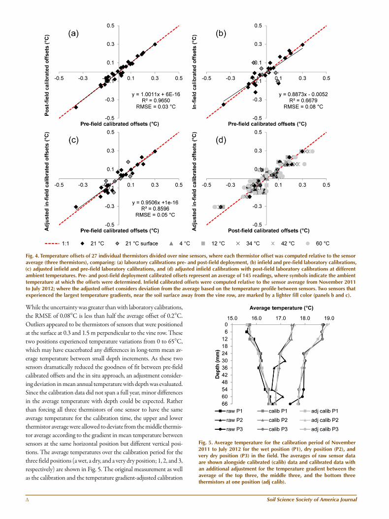
Pre- and Post-Field Laboratory CalibrationAn intercalibration of the thermistors in the laboratory before

and after field deployment, with 5 yr in between (and several field deployments in addition to the dataset described above), indicated that the temperature offsets remained fairly constant with time (Fig. 4a). The RMSE of 0.03°C is an order of magnitude smaller than the average offset of 0.2°C. A comparison between the offsets de-termined in situ and by post-field laboratory is shown in Fig. 4b.

Fig. 3. Average weekly temperature (T) measured by individual thermistors (Th) compared with sensor averages (three thermistors per sensor) over a period stretching from November 2011 through July 2012. Each panel presents temperatures for an individual sensor where x is the horizontal position perpendicular to the vine row and z is the vertical position below the surface. Temperature offsets were calculated as the average deviation of individual thermistors from the sensor average.

∆ Soil Science Society of America Journal

While the uncertainty was greater than with laboratory calibrations, the RMSE of 0.08°C is less than half the average offset of 0.2°C. Outliers appeared to be thermistors of sensors that were positioned at the surface at 0.3 and 1.5 m perpendicular to the vine row. These two positions experienced temperature variations from 0 to 65°C, which may have exacerbated any differences in long-term mean av-erage temperature between small depth increments. As these two sensors dramatically reduced the goodness of fit between pre-field calibrated offsets and the in situ approach, an adjustment consider-ing deviation in mean annual temperature with depth was evaluated. Since the calibration data did not span a full year, minor differences in the average temperature with depth could be expected. Rather than forcing all three thermistors of one sensor to have the same average temperature for the calibration time, the upper and lower thermistor average were allowed to deviate from the middle thermis-tor average according to the gradient in mean temperature between sensors at the same horizontal position but different vertical posi-tions. The average temperatures over the calibration period for the three field positions (a wet, a dry, and a very dry position; 1, 2, and 3, respectively) are shown in Fig. 5. The original measurement as well as the calibration and the temperature gradient-adjusted calibration

Fig. 4. Temperature offsets of 27 individual thermistors divided over nine sensors, where each thermistor offset was computed relative to the sensor average (three thermistors), comparing: (a) laboratory calibrations pre- and post-field deployment, (b) infield and pre-field laboratory calibrations, (c) adjusted infield and pre-field laboratory calibrations, and (d) adjusted infield calibrations with post-field laboratory calibrations at different ambient temperatures. Pre- and post-field deployment calibrated offsets represent an average of 145 readings, where symbols indicate the ambient temperature at which the offsets were determined. Infield calibrated offsets were computed relative to the sensor average from November 2011 to July 2012; where the adjusted offset considers deviation from the average based on the temperature profile between sensors. Two sensors that experienced the largest temperature gradients, near the soil surface away from the vine row, are marked by a lighter fill color (panels b and c).

Fig. 5. Average temperature for the calibration period of November 2011 to July 2012 for the wet position (P1), dry position (P2), and very dry position (P3) in the field. The averages of raw sensor data are shown alongside calibrated (calib) data and calibrated data with an additional adjustment for the temperature gradient between the average of the top three, the middle three, and the bottom three thermistors at one position (adj calib).

www.soils.org/publications/sssaj ∆

are shown, where the variation with depth was largest in the driest position. While the temperature gradient adjustment introduced some additional errors because of uncertainty in the exact distance between sensors, the RMSE improved from 0.08 to 0.05°C and the slope from 0.89 to 0.95 (Fig. 4c).

The mean average temperatures measured over the calibra-tion period were slightly lower than 20°C, but the thermistors were subject to temperatures up to 65°C. An assessment of the effect of ambient temperature on the magnitude of temperature offsets indicated that differences between thermistors tended to increase with increasing temperature (Fig. 4d). On average, the deviation from the sensor average (negative or positive) in-creased by 0.04°C. Some of the error in the in situ calibration results may have been caused by these deviations in offset.

CONCLuSIONAn approach to intercalibrate thermistors for improved esti-

mation of soil temperature gradients in situ was evaluated using heat-pulse sensors under desert conditions. It was found that the thermistors could be calibrated using a constant offset and that changes in offsets over a 5-yr time period were relatively small. Ambient temperature affected the magnitude of the offsets, which tended to increase with increasing temperature, but these chang-es were an order of magnitude smaller than differences between individual thermistors. Laboratory interthermistor calibration prior to or following field deployment can largely account for er-rors in measured temperature gradients and is advisable. When laboratory calibration cannot be conducted, the in situ approach, which improved temperature readings by 0.2°C on average with an RMSE of 0.08°C, is still beneficial. Additional adjustment for temperature gradients between sensors further reduced the RMSE to 0.05°C. Under less extreme environmental conditions, errors after calibration might be even smaller.

ACKNOwLEDGMENTSThis research was supported by Research Grant No. US-4262-09 from BARD, the United States– Israel Binational Agricultural Research and Development Fund, and was partially supported by the I-CORE

Program of the Planning and Budgeting Committee, the Israel Science Foundation (grant no. 152/11), and U.S. NSF Grant No. 1215864.

REFERENCESHam, J.M., and E.J. Benson. 2004. On the construction and calibration of

dual-probe heat capacity sensors. Soil Sci. Soc. Am. J. 68:1185–1190. doi:10.2136/sssaj2004.1185

Heitman, J.L., J.M. Basinger, G.J. Kluitenberg, J.M. Ham, J.M. Frank, and P.L. Barnes. 2003. Field evaluation of the dual-probe heat-pulse method for measuring soil water content. Vadose Zone J. 2:552–560. doi:10.2136/vzj2003.0552

Heitman, J.L., R. Horton, T.J. Sauer, and T.M. DeSutter. 2008. Sensible heat observations reveal soil-water evaporation dynamics. J. Hydrometeorol. 9:165–171. doi:10.1175/2007JHM963.1

Hillel, D. 1998. Environmental soil physics. Academic Press, San Diego, CA.Kojima, Y., J.L. Heitman, G.N. Flerchinger, T. Ren, and R. Horton. 2016.

Sensible heat balance estimates of transient soil ice contents. Vadose Zone J. 15(5):1–11. doi:10.2136/vzj2015.10.0134

Kool, D., N. Agam, N. Lazarovitch, J.L. Heitman, T.J. Sauer, and A. Ben-Gal. 2014a. A review of approaches for evapotranspiration partitioning. Agric. For. Meteorol. 184:56–70. doi:10.1016/j.agrformet.2013.09.003

Kool, D., A. Ben-Gal, N. Agam, J. Šimůnek, J.L. Heitman, T.J. Sauer, and N. Lazarovitch. 2014b. Spatial and diurnal below canopy evaporation in a desert vineyard: Measurements and modeling. Water Resour. Res. 50:7035–7049. doi:10.1002/2014WR015409

Lawton, K.M., and S.R. Patterson. 2001. Long-term relative stability of thermistors. Precis. Eng. 25:24–28. doi:10.1016/S0141-6359(00)00051-9

Lawton, K.M., and S.R. Patterson. 2002. Long-term relative stability of thermistors: Part 2. Precis. Eng. 26:340–345. doi:10.1016/S0141-6359(02)00110-1

Ochsner, T.E., and J.M. Baker. 2008. In situ monitoring of soil thermal properties and heat flux during freezing and thawing. Soil Sci. Soc. Am. J. 72:1025–1032. doi:10.2136/sssaj2007.0283

Peng, X., J. Heitman, R. Horton, and T. Ren. 2015. Field evaluation and improvement of the plate method for measuring soil heat flux density. Agric. For. Meteorol. 214–215:341–349. doi:10.1016/j.agrformet.2015.09.001

Ren, T., K. Noborio, and R. Horton. 1999. Measuring soil water content, electrical conductivity, and thermal properties with a thermo-time domain reflectometry probe. Soil Sci. Soc. Am. J. 63:450–457. doi:10.2136/sssaj1999.03615995006300030005x

Sauer, T.J., and R. Horton. 2005. Soil heat flux. In: M.K. Viney, J.L. Hatfield, and J.M. Baker, editors, Micrometeorology in Agricultural Systems. Agron. Monogr. 47. Madison, WI. p. 131–154. doi:10.2134/agronmonogr47.c7

Wilcox, B.P., D.D. Breshears, and M.S. Seyfried. 2003. Rangelands, water balance on. In: B.A. Stewart and T.A. Howell, editors, Encyclopedia of water science. Marcel Dekker, Inc., New York. p. 791–794.

Wood, S.D., B.W. Mangum, J.J. Filliben, and S.B. Tillett. 1978. An investigation of the stability of thermistors. J. Res. Natl. Bur. Stand. 83(3):247–263. doi:10.6028/jres.083.015