Soil Moisture Active Passive

In Situ Sensor Testbed

Experiment Plan

ver. 4/1/2010

2

Table of Content 1. Background ........................................................................................................... 3 2. Study Site ............................................................................................................... 5 3. Experiment Design................................................................................................ 6

3.1 Sensor Comparison .............................................................................................. 6 3.2 Sampling Scales ................................................................................................... 8 3.3 Sampling Intervals ............................................................................................... 8

4. Ground Support and Ancillary Data Plans ........................................................ 9 4.1. Ground Soil Moisture Measurement Campaign ................................................... 9 4.2. Vegetation Water Content................................................................................... 9 4.3. Surface Roughness............................................................................................... 9 4.4. Soil Characterization.......................................................................................... 10

5. In Situ Sensors..................................................................................................... 11 5.1. Stevens Water Hydra Probe ............................................................................... 11 5.2. Delta-T Theta Probe........................................................................................... 13 5.3. Decagon ECHO EC-TM Probe.......................................................................... 15 5.4. Sentek EnviroSMART Capacitance Probe ........................................................ 15 5.5 Campbell CS615/CS616 Time Domain Reflectometer ..................................... 16 5.6 CS 229-L Heat Dissipation sensors ................................................................... 17 5.7 Acclima .............................................................................................................. 18 5.8 Other TDR ......................................................................................................... 19 5.9 Passive Distributed Temperature Sensing (DTS) .............................................. 19 5.10 GPS Reflectometry ............................................................................................ 19 5.11 The Cosmic-ray Soil Moisture Observing System (COSMOS) ........................ 20 5.12 Mongolian Soil Moisture Station....................................................................... 21 5.13 Climate Reference Network Stations................................................................. 21

6. Sampling Protocols ............................................................................................. 23 6.1. General Guidance on Field Sampling ............................................................... 23 6.2. Station Validation ............................................................................................. 23 6.4 Theta Probe Soil Moisture Sampling and Processing....................................... 25 6.5 Gravimetric Soil Moisture Sampling with the Scoop Tool .............................. 32 6.6 Gravimetric Soil Moisture Sample Processing ................................................. 33 6.7 Soil Bulk Density and Surface Roughness ....................................................... 33 6.8 Soil Temperature Probes................................................................................... 38 6.9 Hydra Probe Soil Moisture Installations........................................................... 39 6.10 Vegetation Sampling......................................................................................... 40

7 Logistics ............................................................................................................... 55 7.1 Security/Access to Fields.................................................................................. 55 7.3 Local Contacts and Shipping ............................................................................ 56

8. References............................................................................................................ 57

3

1. Background The Soil Moisture Active Passive Mission (SMAP) is currently in Phase A and addressing numerous issues related to the L3 soil moisture retrieval algorithms. During discussions at the SMAP Workshop in June 2009, issues related to calibration and validation of the soil moisture product were discussed and some key questions regarding how current and future networks resources, shown in Table 1.1, could be integrated were identified. They included. • How do different sensors perform given the same hydrologic inputs of rainfall and

evaporation? • How can the measurements from different sensors with different sampling scales,

particularly the COSMOS and GPS systems of soil moisture monitoring, compare given the variation in scale of measurement?

• How do different sampling intervals impact the soil moisture estimates, given instantaneous measurements versus time averaged measurements?

• How can networks which measure soil moisture by different fundamental methods, capacitance, FDR, TDR, reflectometry, be compared to a standard of gravimetric validation?

• How do the orientations of installation influence the data record and effectiveness of the sensor?

Addressing these issues as soon as possible would contribute to calibration and validation planning, design, and selection. It was determined that an In Situ Sensor Testbed would be developed to study these different questions. Criteria were developed so that the testbed would best mimic the average long term in situ soil moisture stations. These included: • Minimum scale of 700 m of same landuse • Rangeland/Pasture site • Low Topography • Deep soil profile (at least 1 meter of soil • Long term access through 2016 • Local scientist who can conduct sampling and provide maintenance • Range of moisture conditions After reviewing several locations and evaluating their advantages, a location near Marena Oklahoma was selected and research relationships established with Oklahoma State University, and the University of Oklahoma/Mesonet. Installation of the testbed is planned for Spring of 2010 with an expected duration of 6 years.

4

Table 1.1: In Situ instrumentation for soil moisture monitoring. Network # Stations Primary Sensor Secondary Sensor Little Washita, OK, USA 20 Hydra (5, 25, 45 cm) Little River, GA, USA 29 Hydra (5, 15, 30 cm) Reynolds Creek, ID USA 19 Hydra (5 cm) Walnut Gulch, AZ USA 21 Hydra (5 cm ) + Walnut Creek, IA USA 9 Hydra (5 cm) Fort Cobb, OK USA 15 Hydra (5, 25, 45 cm) St. Joe's Watershed, IN USA 6 Hydra (5, 20, 40, 60 cm) SCAN, USDA, USA 151 Hydra (5, 10, 20, 50, 100cm)

CRN, NOAA, USA 114 Hydra (5, 10, 20, 50, 100cm) with 3 replicates

Oklahoma Mesonet, OK USA 127 CS 229-L heat dissipation sensor ( 5, 25, 60, 75 cm)

High Plains Regional Climate Center, NE USA 53 Theta (10, 25, 50, 100 cm)

Arizona Soil Moisture Network 5 5 TDR (5, 10, 20, 50, 100 cm) 1 Hydra (5, 10, 20, 50, 100 cm)

Illinois Water Survey, IL USA 19 Hydra (5, 10, 20, 50, 100, 150 cm)

SGP-ARM-CART, OK USA 31

CS 229-L heat dissipation sensor ( 5, 15, 25, 35, 60, 85, 125, 175 cm)

Sonora, Mexico 14 Hydra (5 cm) Mongolia 17 TDR (3, 10, 40, 100) variable Salamanca, Spain (REMEDHUS) 24 TDR (5, 10, 15, 25, 50) Hydra(5cm) Spain, Valencia ~9 Theta (5cm) Hydra (5 cm)

Australia 39 CS615 (4, 15, 45, 75 cm) / CS616 (15, 45, 75 cm) Hydra 2.5cm

COPS-Germany Simplified Soil Moisture Probe (SISOMOP)

SMOS-Fit 10 TDR (IMKO TRIME-ES) 0-50 at 5 depths

Goulburn, Aus 26 CS616 (15, 45, 75 cm) Hydra 2.5 cm SMOSMANIA-France 12 ThetaProbe(5, 10, 20, 30 cm) Ontario, Canada 16 Hydra (5, 20, 50 cm) Saskatchewan, Canada 15 Hydra (5, 20, 50 cm) Asia 20 TDR (3, 10, 40, 100) variable CERN (Chinese Ecosystem Research Network) 31

Neutron Probe (0-150 cm, every 10 cm)

NEON 20 bore hole (capacitance, and hydras)

AMMA-CATCH, Africa 10 CS616 (5 cm then var., 30, 60, 120, 150, 250, 400)

Skjern River Catchment, Denmark 30

Decagon ECH20 (5, 50 cm + intermediate)

Fluxnet ~500 TDR Korea 2 Hydra (10, 30, 60 cm) COSMOS 50 COSMOS Device GPS Reflectometry GPS Stations CEOP 13 CS615 4, 8, 20 cm Various

5

2. Study Site The region selected for SMAP-ISST is a rangeland region of Oklahoma near Marena. The corner coordinates of the primary study area are listed in Table 2.1. The general location is shown in Figure 2.1.

Table 2.1. Marena Study Area Corner Latitude (Deg.) Longitude (Deg.)

Upper Left 36.069 -97.221 Upper Right 36.069 -97.212 Lower Left 36.058 -97.221 Lower Right 36.058 -97.212

Figure 2.1. Landsat TM False Color Composite of the Marena Site (Aug, 8, 2001). The discoloration is a recent burn of the vegetation which is conducted as part of the land

management plan for the site. This location is managed by the Oklahoma State University Range Research Management Station and contains the MARE station of the Oklahoma Mesonet which has a long term lease. It is a grazed cattle pasture. The soil is sandy clay loam/loam. There is a fence bisecting the field and some terracing to prevent erosion. Sections of the field are burned for salt cedar control every three years with the next scheduled burn to take place in 2012. There is a small amount of topography.

MARE Mesonet

6

3. Experiment Design

There are four key questions to be addressed by this experiment: • How do different sensors perform given the same hydrologic inputs of rainfall and

evaporation? • How can the measurements from different sensors with different sampling scales,

particularly the COSMOS and GPS systems of soil moisture monitoring, compare given the variation in scale of measurement?

• How do different sampling intervals impact the soil moisture estimates, given instantaneous measurements versus time averaged measurements?

• How can networks which measure soil moisture by different fundamental methods, capacitance, FDR, TDR, TDT, reflectometry, be compared to a standard of gravimetric validation?

3.1 Sensor Comparison

In order to compare the sensors, it is necessary to have a suite of sensors in the same location. Redundancy is also desirable, therefore, a common configuration of sensors will be employed at multiple locations in the location.

Table 3.1: Configurations of the Base in situ station

Configuration Depths Stevens Water Hydra Probe 2.5, 5, 10, 20, 50, 100 cm Delta-T Theta Probe 5, 10, 20, 50, 100 cm EC-TM Probe 5, 10, 20, 50, 100 cm EnviroSMART 10 , 20, 50, 100 cm Acclima 5, 10, 20, 50, 100 cm CS229-L Heat Dissipation Sensor 5, 10, 20, 50, 100 cm CS616s TDR 5, 10, 20, 50, 100 cm ASSH-TRIME (2 stations) 3, 5, 10 cm

This Base station will be used as the main sensor station for the testbed with a total of four being deployed in the field. Figure 3.1 contains a tentative diagram of the deployment at four stations. Additional instrumentation will also be deployed given the with a tentative deployment scheme shown in Table 3.2. Approximate locations are listed in Table 3.3. There will be one COSMOS station located at Site A. There may be as many as 3 GPS reflectometers located in the testbed with one located on a tower at the central site (Site A). A passive DTS system will be deployed between Sites A and B at a depth of 10 cm. Two stations will be deployed by NOAA which will replicate the Climate Reference Network stations. At these locations, the Hydra installation at the Base stations may be reconfigured to 3 sensors at 2.5 cm and 3 at 5 cm, to provide a higher degree of replication at the shallow layer. Traditional TDR systems and a system from Mongolia will also be deployed but may be added at a later date, depending on logistics. Figure 3.2 shows the relative distances between these sites. Table 3.2 shows how the different sites will be configured.

7

Figure 3.1: Tentative configuration with Testbed sites A-D represented by red hexagons.

The OK Mesonet MARE site is shown as a blue hexagon. Between A and B is the tentative location of the Passive DTS.

Table 3.2: A tentative list of station locations for the testbed. Base refers to the base

station described in Table 3.1. Site A

Site B Site C Site D

Base Base Base Base

GPS Passive DTS GPS GPS

COSMOS ASSH CRN

ASSH

TDR system

Table 3.3: Approximate location of in situ stations in WGS84.

Site Latitude Longitude A 36.06348 -97.21693 B 36.06168 -97.21735 C 36.06353 -97.21777 D 36.06520 -97.21507

A

B

C

DMARE

DTS

8

Figure 3.2: Dimensions of the various sites in comparison to the central site. This will

help define the sampling domain for the periodic gravimetric sampling.

3.2 Sampling Scales

There are three primary scales of interest in this study, 5-10 cm (Hydra, Theta, EC-TM, EnviroSMART, TDR, 229-L), 1 m (GPS reflectometers), and 700 m (COSMOS). To address these scale differences, the soil moisture measurement stations will be distributed throughout a 700 m diameter footprint with the COSMOS station at the center. These four stations will be distributed at the following intervals, 0 m, 100 m, 200 m, and 300 m away from the center. At 400 m from the site, there will be an Oklahoma Mesonet station (MARE). The radial direction will be determined in consideration of the local topography and vegetation. Gravimetric sampling will be conducted throughout the field at these scales on a monthly basis (not winter), to understand how each scale varies in soil moisture magnitude.

3.3 Sampling Intervals The method of sampling interval or averaging will be addressed by a simple statistical post-processing. Common sampling intervals for these instruments are one instantaneous samples every 1 hour, while some others average samples for several minutes. To accommodate this investigation, the sampling interval for most of the sensors will be increased to 1 min for 5 minutes at the top of each hour. This investigation will seek to quantify the short temporal variability of the sensor measurements.

3.4 Gravimetric comparisons

Monthly gravimetric collection of soil moisture will be conducted to provide ground truth to the in situ measurements. Both surface and depth measurements will be made to provide a quality data set of the evolution of soil moisture throughout the domain.

300 m400 m

200 m

100 m

9

4. Ground Support and Ancillary Data Plans Soil moisture sampling will include concurrent observations of agricultural fields using Theta probes and gravimetric sampling. Protocols for sampling are included in Section 8. 4.1. Ground Soil Moisture Measurement Campaign The goal of soil moisture sampling in the In Situ Testbed is to provide a reliable estimate of the mean and variance of the volumetric soil moisture within the field domain. Specific methodologies will evolve during the experiment as the ongoing results lead evolving sampling strategies. The primary measurement made will be the 0-6 cm gravimetric sampling coupled with 0-6 cm dielectric constant (voltage) at multiple locations using the Theta Probe (TP). Initial locations will be co-located with any in situ instrumentation installed in the field. Additional details will be provided in the Protocols section of the experiment plan. Dielectric constant is converted to volumetric soil moisture using a calibration equation. There are built in calibration equations and, as the result of SMEX02 and SMEX03 studies (Cosh et al., 2005), site specific calibrations have proven reliable. GSM is converted to volumetric soil moisture (VSM) by multiplying gravimetric soil moisture by the bulk density of the soil. Bulk density will be sampled one time at multiple locations in the field, to provide a conversion parameter, using an extraction technique. These coincident gravimetric samples will provide a ground truth for Theta Probe calibration activities. Theta probes consist of a waterproof housing which contains the electronics, and, attached to it at one end, four sharpened stainless steel rods that are inserted into the soil. The probe generates a 100 MHz sinusoidal signal, which is applied to a specially designed internal transmission line that extends into the soil by means of the array of four rods. The impedance of this array varies with the impedance of the soil, which has two components - the apparent dielectric constant and the ionic conductivity. Because the dielectric of water (~81) is very much higher than soil (typically 3 to 5) and air (1), the dielectric constant of soil is determined primarily by its water content. The output signal is 0 to1V DC for a range of soil dielectric constant, ε, between 1 and 32, which corresponds to approximately 0.5 m3 m-3 volumetric soil moisture content for mineral soils. More details on the probe are provided in the sampling protocol section of the plan. 4.2. Vegetation Water Content Vegetation biomass sampling will be performed at different stages of the study period to provide a reference for measurement techniques which may be affected by vegetation water content. The primary measurements of vegetation are: 1) Leaf Area Index (LAI), 2) vegetation water content, and 3) multispectral observations made with a Cropscan instrument, described in the protocol sections when available. 4.3. Surface Roughness

10

Each year, the site will be characterized for surface roughness. The grid board photography method employed in previous experiments will be used. A total of five locations will be selected in a field. Between two and four pictures will be taken at each location to insure data capture and one pair of images will be processed for xy directions. 4.4. Soil Characterization A detailed characterization of the soil profile will be collected for the domain down to a depth of 1 meter collected during station installation. Variables of important include dielectric constant of dry soil, texture, percent sand, percent clay, bulk density, and rock fraction.

11

5. In Situ Sensors The primary purpose of the testbed is to compare various in situ sensors which are in use throughout the U.S. and world, as shown in Table 1.1. From this list of sensors, a subset was selected. Additional instrumentation will be installed as the need arises. 5.1. Stevens Water Hydra Probe

Figure 5.1: The Stevens Hydra Probe Head

The Stevens Hydra Probe II soil sensor is an in-situ soil probe that measures 21 different soil parameters simultaneously with digital output. The Hydra Probe II soil sensor calculates soil moisture, electrical conductivity/salinity, and temperature as well as supplying voltage outputs for research applications. The Hydra Probe provides accurate and precise measurements. Table 5.1 below shows the accuracy and precision statistics. Table 5.1 Accuracy and Precision of the Hydra Probes’ Parameters. *TUC Temperature uncorrected full scale, **TC Temperature corrected from 0 to 35o C

Parameter Accuracy/Precision Temperature (C) +/- 0.6 Degrees Celsius(From -10o to

36oC) Soil Moisture wfv (m3 m-3) +/- 0.03 wfv (m3 m-3) Accuracy Soil Moisture wfv (m3 m-3) +/- 0.003 wfv (m3 m-3) Precision Electrical Conductivity (S/m) TUC* +/- 0.0014 S/m or +/- 1% Electrical Conductivity (S/m) TC** +/- 0.0014 S/m or +/- 5% Real/Imaginary Dielectric Constant TUC* +/- 0.5 or +/- 1% Real/Imaginary Dielectric Constant TC* +/- 0.5 or +/- 5%

Typical installation of the sensor is horizontally into an undisturbed soil profile, as shown in Figure 5.1. The sensing volume for the sensor is cylindrical and is oriented around the metal tines.

12

Figure 5.2: Installation of an array of Hydra probes in a soil profile. The wires are sealed

in metal conduit wire to protect from vermin, and the hole will be backfilled with the excavated soil so as not to create preferential pathways for water to percolate.

The cylindrical measurement region or sensing volume is the soil that resides between the stainless steel tine assembly. The tine assembly is often referred to as the wave guide and probe signal averages the soil in the sensing volume.

Table 5.2 Physical description of the Hydra Probe (All Versions)

Feature Attribute Probe Length 12.4 cm (4.9 inches) Diameter 4.2 cm (1.6 inches) Sensing Volume* (Cylindrical measurement region)

Length 5.7 cm (2.2 inches) Diameter 3.0 cm (1.2 inches)

Weight 200g (cable 80 g/m) Power Requirements 7 to 20 VDC (12 VDC is ideal) Temperature Range -10 to 65o C Storage Temperature Range -40 to 70o C

The defined sensing area allows accurate measurements in regions where there are strong soil moisture gradients, such as near the soil surface. Response time to changing soil conditions is immediate, and calibration is as simple as selecting a soil type (sand, silt, loam or clay). Each Hydra Probe is serial addressable, allowing for multiple sensors to be connected to any RS485 or SDI-12 data logger via a single cable. Sensor data can also be sent directly to a radio modem through a small RS485-RS232 converter. The Hydra Probe uses an electromagnetic signal propagated from the center tine of the probe to measure multiple parameters. The voltages recorded depend on the type of electrical properties of the soil. On-board software converts the raw voltage to standard units of measurement for each parameter. With a standard database or spreadsheet, managers can view real-time soil snapshots or long-term soil trends.

13

5.2. Delta-T Theta Probe

Figure 5.3: The ThetaProbe ML2x

The ThetaProbe measures volumetric soil moisture content, θv, by the well established method of responding to changes in the apparent dielectric constant. These changes are converted into a DC voltage, virtually proportional to soil moisture content over a wide working range. Volumetric soil moisture content is the ratio between the volume of water present and the total volume of the sample. This is a dimensionless parameter, expressed either as a percentage (%vol), or a ratio (m3.m-3). Thus 0.0 m3.m-3 corresponds to a completely dry soil, and pure water gives a reading of 1.0 m3.m-3. There are important differences between volumetric and gravimetric soil moisture contents.

Figure 5.4: Design of the Theta Probe

14

Calibration of the Theta Probe is recommended using the following equation.

[ ]1

032 7.44.64.607.1

aaVVV −+−+

=θ

Using a0 and a1 as tuning parameters, to minimize the errors between the ThetaProbe soil moisture estimate and gravimetric samples.

Table 5.4: Factory Calibrations for the Theta Probe ML2x a0 a1 Mineral Soils 1.6 8.4 Organic Soils 1.3 1.7

Table 5.3: Technical Specifications for the Theta Probe ML2x

Measurement parameter Volumetric soil moisture content, θV (m3.m-3 or %vol.). Range Accuracy figures apply from 0.05 to 0.6 m3.m-3 , Full range is

from 0.0 to 1.0 m3.m-3

±0.01 m3.m-3 , 0 to 40°C, ±0.02 m3.m-3 , 40 to 70°C, after calibration to a

specific soil type

Accuracy subject to soil salinity errors, see below

±0.05 m3.m-3 , 0 to 70°C using the supplied soil calibration, in all 'normal' soils,

Soil salinity errors 0.0 to 250 mS.m-1 , < -0.0001 m3.m-3 change per mS.m-1 , 250 to 2000 mS.m-1, no significant change.

Soil sampling volume >95% influence within cylinder of 4.0cm diam., 6cm long, (approx 75 cm3 ), surrounding central rod.

Environment Will withstand burial in wide ranging soil types or water for long periods without malfunction or corrosion (IP68 to 5m)

Stabilization time 1 to 5 sec. from power-up, depending on accuracy required.

Response time Less than 0.5 sec. to 99% of change.

Duty cycle 100 % ( Continuous operation possible ). Interface

Input requirements: 5-15V DC unregulated. Current consumption: 19mA typical, 23mA max. Output signal: approx. 0-1V DC for 0-0.5m3m -3

Case material PVC

Rod material Stainless steel

Cable length Standard: 5m. Maximum length: 100m Weight 350 gm approx. with 5m cable.

15

5.3. Decagon ECHO EC-TM Probe

Figure 5.5: The Decagon EC-TM soil moisture probe

The EC-TM obtains volumetric water content by measuring the dielectric constant of the media through the utilization of capacitance/frequency domain technology. In addition, the EC-TM sensors incorporate a high frequency oscillation, which allows the sensor to accurately measure soil moisture in any soil or soilless media with minimal salinity and textural effects. The design of the EC-TM allows the sensor to be pushed directly into undisturbed soil. Table 5.5: Technical Specifications for the Decagon ECH2O EC-TM Probe Accuracy: Mineral Soil

±3% VWC, All mineral soils ±1-2% VWC soil specific calibration

Resolution: ~0.1% VWC (mineral soil) Range: 0-100% VWC Measurement Time: 150 ms Power: 3.6-15 V @ 10 mA Output: SDI-12 Temperature: -40°C to +50°C 5.4. Sentek EnviroSMART Capacitance Probe

EnviroSCAN Solo is a cost effective, continuous soil moisture and salinity monitoring solution. The system consists of a battery powered, logging probe connected to a Head Unit, which allows for in-field download via a laptop or SoloPORTER. The data captured is displayed in Sentek’s IrriMAX software, allowing for user friendly measurement and management of data. Compatible with TriSCAN sensors, EnviroSMART and EasyAG probes, EnviroSCAN Solo is suitable for a range of applications. EnviroSCAN Solo provides an economical way for Diviner 2000 users to upgrade into continuous soil moisture monitoring. EnviroSCAN Solo is also easily upgradeable to EnviroSCAN Plus for web compatible, wireless communication and other EnviroSMART interfaces for

16

third party telemetry options. EnviroSCAN Solo combines the proven sensor technology of the world’s most used soil water monitoring solution, EnviroSCAN.

Figure 5.6: The internal structure of the Sentek EnviroSMART.

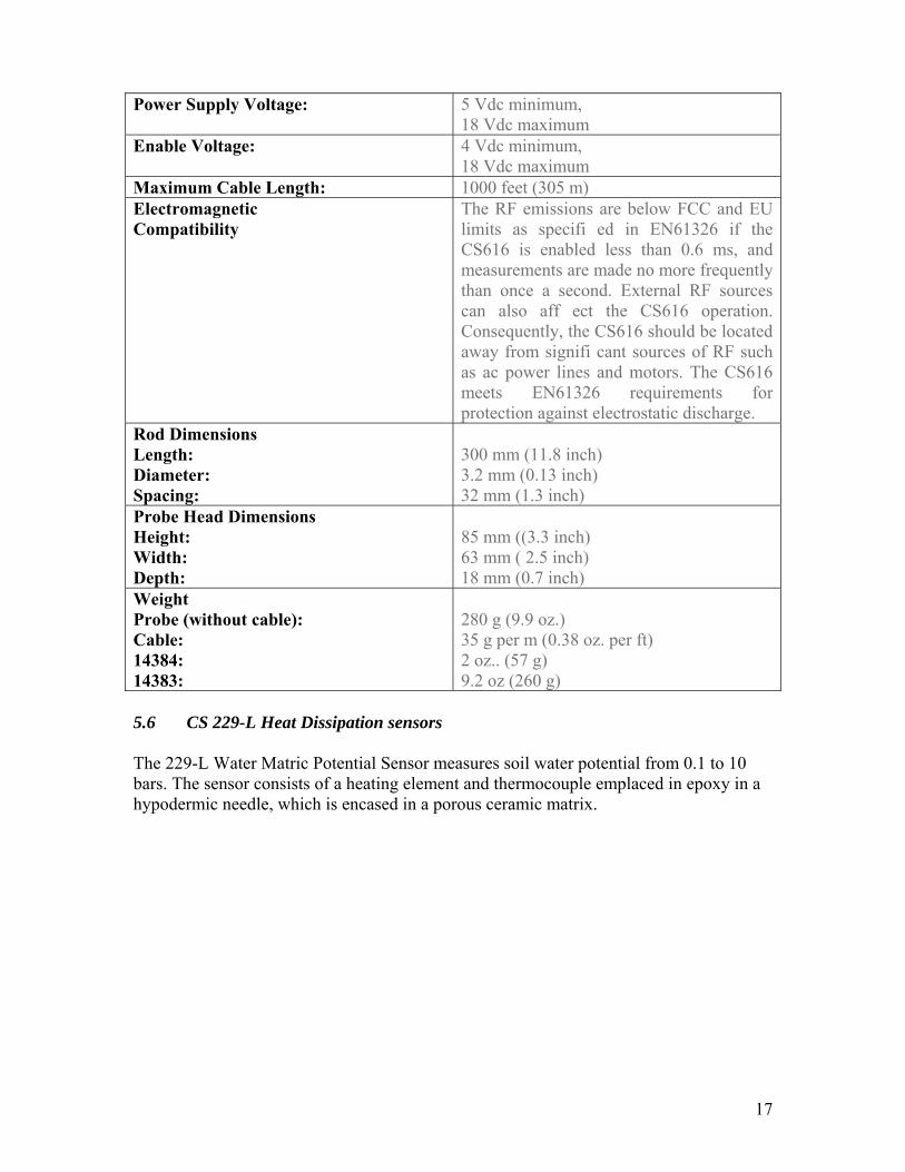
5.5 Campbell CS615/CS616 Time Domain Reflectometer The CS616 Water Content Reflectometer measures the volumetric water content of porous media using time-domain measurement methods that are sensitive to dielectric permittivity. The probe consists of two 30 cm long stainless steel rods connected to a printed circuit board. The circuit board is encapsulated in epoxy, and a shielded four-conductor cable is connected to the circuit board to supply power, enable probe, and monitor the output. The probe rods can be inserted from the surface or the probe can be buried at any orientation to the surface. The CS616 connects directly to one of the datalogger’s single-ended analog inputs. A datalogger control port enables the CS616 for the amount of time required to make the measurement. Datalogger instructions convert the probe square-wave output to a period which is converted to volumetric water content using a calibration.

Figure 5.7: The probe head and rods of the Campbell CS616 Time Domain Reflectometer Table 5.6: Technical Specifications for the Campbell CS616 Time Domain Reflectometer. Output: ±0.7 volt square wave with

frequency dependent on water content

Power: 65 mA @ 12 Vdc when enabled, 45 μA quiescent typical

17

Power Supply Voltage: 5 Vdc minimum, 18 Vdc maximum

Enable Voltage: 4 Vdc minimum, 18 Vdc maximum

Maximum Cable Length: 1000 feet (305 m) Electromagnetic Compatibility

The RF emissions are below FCC and EU limits as specifi ed in EN61326 if the CS616 is enabled less than 0.6 ms, and measurements are made no more frequently than once a second. External RF sources can also aff ect the CS616 operation. Consequently, the CS616 should be located away from signifi cant sources of RF such as ac power lines and motors. The CS616 meets EN61326 requirements for protection against electrostatic discharge.

Rod Dimensions Length: Diameter: Spacing:

300 mm (11.8 inch) 3.2 mm (0.13 inch) 32 mm (1.3 inch)

Probe Head Dimensions Height: Width: Depth:

85 mm ((3.3 inch) 63 mm ( 2.5 inch) 18 mm (0.7 inch)

Weight Probe (without cable): Cable: 14384: 14383:

280 g (9.9 oz.) 35 g per m (0.38 oz. per ft) 2 oz.. (57 g) 9.2 oz (260 g)

5.6 CS 229-L Heat Dissipation sensors

The 229-L Water Matric Potential Sensor measures soil water potential from 0.1 to 10 bars. The sensor consists of a heating element and thermocouple emplaced in epoxy in a hypodermic needle, which is encased in a porous ceramic matrix.

18

Figure 5.8: The Campbell Scientific 229-L Heat Dissipation Sensor which measures soil

matric potential. Table 5.7: Technical Specifications of the CS 229-L heat dissipation sensor

Measurement range: -10 to -2500 kPa Measurement time: 30 seconds typically Thermocoupl type: Copper/constantan (type T) Dimensions 1.5 cm diameter

3.2 cm length of ceramic cylinder 6.0 cm length of entire sensor

Weight: 10 g plus 23 g/m of cable Heater resistance 34 ohms plus cable resistance Resolution: ~1 kPa at matric potentials greater than -100 kPa

To calculate soil water matric potential, a Current Excitation Module applies a 50 mA current to the 229's heating element, and the 229 thermocouple measures the temperature rise. The magnitude of the temperature rise varies according to the amount of water in the porous ceramic matrix, which changes as the surrounding soil wets and dries. Soil water matric potential is determined by applying a second-order polynomial equation to the temperature rise. Users must individually calibrate each of their 229 sensors in the soil type in which the sensors will reside. 5.7 Acclima The Acclima is a Time Domain Transmission soil moisture sensor which sends a pulse of electricity through the outer rod of the submerged sensor. As this pulse travels the rod, it is delayed by the moisture content of the soil and distorted by the soil chemistry. As the pulse reaches the other end of the rod, it is digitized at 25 Pico second intervals (about how long it takes light to travel .3 inches). A proprietary digital signal processing system then extracts the critical information.

19

Figure 5.9: The Acclima TDT sensor

5.8 Traditional TDR There is a significant history of time domain reflectometry (TDRs) for soil moisture monitoring. Many long term networks still include TDRs, therefore, one profile of traditional TDR probes will be incorporated into the testbed. The configuration and specifications are still in development. 5.9 Passive Distributed Temperature Sensing (DTS) Passive Soil DTS is an experimental method of measuring soil moisture based on Distributed Temperature Sensing (DTS). Several fiber-optic cables in a vertical profile are buried below the surface and used as thermal sensors, measuring propagation of temperature changes due to the diurnal cycle. Current technology allows these cables to be in excess of 10 km in length, and DTS equipment allows measurement of temperatures every 1m. The Passive Soil DTS concept is based on the fact that soil moisture influences soil thermal properties. Therefore, observing temperature dynamics can yield information on changes in soil moisture content. Deriving soil moisture is complicated by the uncertainty and non-uniqueness in the relationship between thermal conductivity and soil moisture. A numerical simulation indicates that the accuracy could be improved if the depth of the cables was known with greater certainty. This is included as a potential future network technology. 5.10 GPS Reflectometry Global Positioning System (GPS) radio-navigation signals strongly reflect from [liquid] water and, to a lesser extent, from land surfaces. The strength of the land-reflected signal is a function of both surface roughness and dielectric constant. As shown in Figure 8, the airborne GPS Reflectometer is used to simultaneously acquire both the direct-from-satellite and surface-reflected signals. Surface-reflected signals emanate from elliptically shaped areas of constant transmission path delay which yields a power vs. delay map of the surface. Note that this configuration of transmitter (satellites) and physically separate receiver (Reflectometer) form a type of bi-static radar system. The ratio of reflected-to-direct signal power is proportional to surface reflectivity and, allowing for roughness and utilizing appropriate surface models, to surface dielectric constant. The Global Positioning System Reflectometer (GPSR) will fly on the NASA P3-B aircraft.

20

Figure 5.10: Example of a GPS Reflectometer installation.

5.11 The Cosmic-ray Soil Moisture Observing System (COSMOS)

The method involves measuring low-energy cosmic-ray neutrons above the ground, whose intensity is inversely correlated with soil water content and with water in any form above ground level (Note: the contributions from subsurface and surface waters are distinguishable). The following data will be available to all in near-real time over the internet: neutron counts in two energy bands (fast, >1 keV; and thermal, <0.5 eV), soil water content, snow pack water equivalent (and possibly also vegetation water equivalent), temperature, pressure and relative humidity.

Figure 5.11: A COSMOS installation.

The measurements are insensitive to soil chemistry, texture, topography. The system is non-invasive, no contact measurement (probe above the ground measures neutrons emitted from soil).It is fully automatic measurement and data transfer. The estimated measurements are of integrated soil moisture over a footprint of ~700 m, over a depth 0-70 cm (dry) and 0-12 cm (wet). The precision is based on the number of counts (2%

21

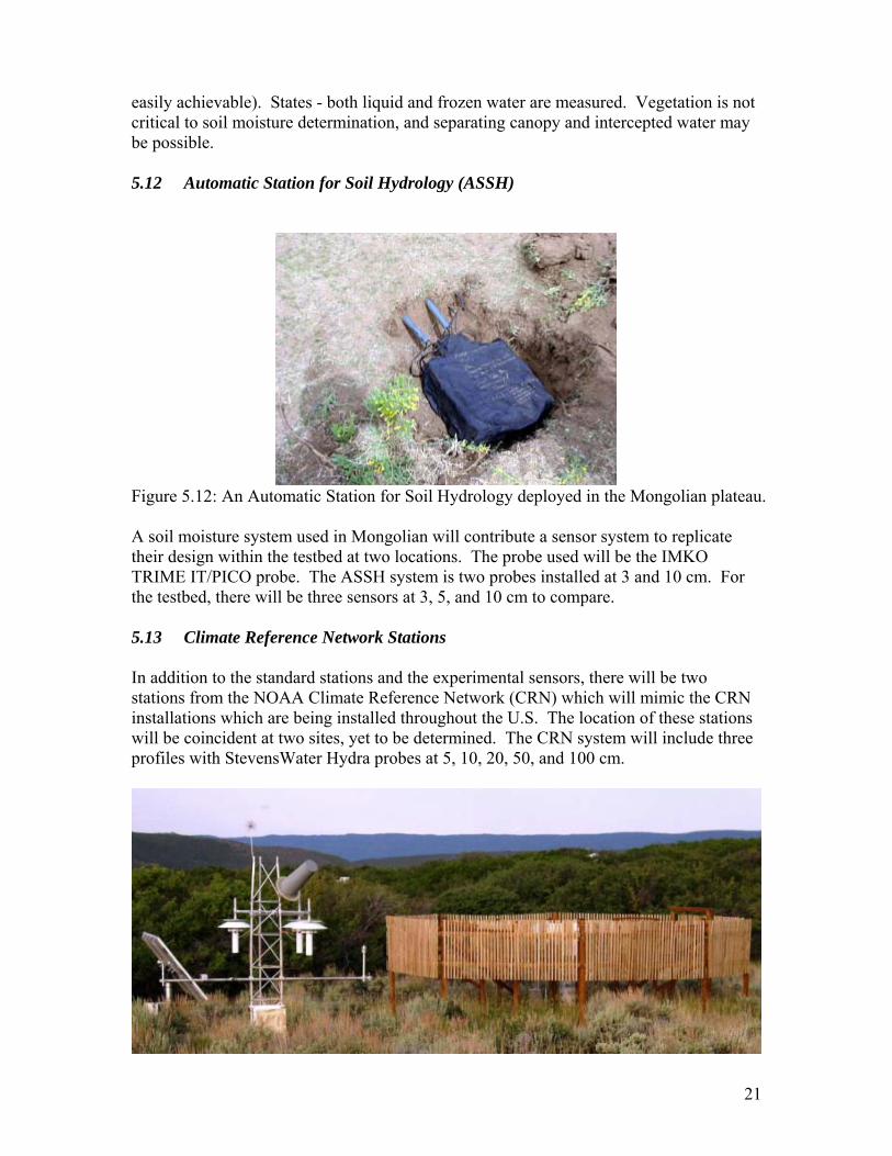
easily achievable). States - both liquid and frozen water are measured. Vegetation is not critical to soil moisture determination, and separating canopy and intercepted water may be possible. 5.12 Automatic Station for Soil Hydrology (ASSH)

Figure 5.12: An Automatic Station for Soil Hydrology deployed in the Mongolian plateau.

A soil moisture system used in Mongolian will contribute a sensor system to replicate their design within the testbed at two locations. The probe used will be the IMKO TRIME IT/PICO probe. The ASSH system is two probes installed at 3 and 10 cm. For the testbed, there will be three sensors at 3, 5, and 10 cm to compare. 5.13 Climate Reference Network Stations In addition to the standard stations and the experimental sensors, there will be two stations from the NOAA Climate Reference Network (CRN) which will mimic the CRN installations which are being installed throughout the U.S. The location of these stations will be coincident at two sites, yet to be determined. The CRN system will include three profiles with StevensWater Hydra probes at 5, 10, 20, 50, and 100 cm.

22

Figure 5.13: A typical NOAA Climate Reference Network Station

23

6. Sampling Protocols 6.1. General Guidance on Field Sampling • Although gravimetric and vegetation sampling are destructive, try to minimize your

impact by filling holes. Leave nothing behind. And try not to disturb the ‘soil moisture patterns’ of the field.

• Please be considerate of the landowners and our hosts. Don’t block roads, gates, and driveways. Keep sites, labs and work areas clean of trash and dirt.

• Watch your driving speed, especially when entering towns. Be courteous on dirt and gravel roads, lower speed=less dust.

• Avoid parking in tall grass, catalytic converters can be a fire hazard. • Close any gate you open as soon as you pass. • Work in teams of two. Carry a cell phone. 6.2. Station Validation Soil moisture sampling at the stations is designed to determine the local soil moisture average near each ground station. For each day of sampling the following measurements will be taken at each in situ station, including the Mesonet. • 20 0-6 cm soil moisture using the Theta Probe (TP) instrument • 5 0-6 cm gravimetric soil moistures using the scoop tool coincident with theta probe • 5 cm soil temperature • GPS locations of all sample point locations • 3 cores from 0-100 cm with soil moisture measurements taken at 5, 10, 20, 50, and

100 cm with a theta probe. • Use a new notebook page each day. Take the time to draw a good map and be

legible. These notebooks belong to the experiment; if you want your own copy make a photocopy.

24

6.3 Large Scale Validation

Figure 6.1: Sampling scheme for the Radial Large Scale Validation with sampling every

50 m. To capture the large scale variability of the domain, a series of transects will be sampled. The size of field of interest is 700 m with a focus on concentric patterns. • Starting at the central station where COSMOS is located, sample every 50 m in on

direction out to 350 m. Then transverse 200 m and proceed back to the central station. Each transect to radiate out and a total of 8 transects from the center.

• At each sampling point, collect 3 theta probe measurements and a gravimetric sample at the 2nd theta probe sampling point.

• As you move along the transect note any anomalous conditions on the schematic in your notebook, i.e. standing water.

• Record your stop time and place cans in box.

25

Figure 6.2. Schematic of layout of Theta Probe sample points in a field with row

structure.

Sample Data Processing • Return to the field headquarters immediately upon finishing sampling. Do not leave

something until the next day. • For each site, weigh the gravimetric samples and record on the oven data sheets that

will be provided. Use a single data sheet for all your samples for that day and record cans sequentially.

• Clean your other equipment. 6.4 Theta Probe Soil Moisture Sampling and Processing There are two types of TP configurations; Type 1 (Rod) (Figure 6.3) and Type 2 (Handheld) (Figure 6.4). They are identical except that Type 1 is permanently attached to the extension rod.

Figure 6.3. Theta Probe Type 1 (with extension rod).

Tractor Row

SamplingRow

Theta ProbeSample Points

Tractor Row

SamplingRow

Theta ProbeSample Points

26

Figure 6.4. Theta Probe Type 2. TPs consist of a waterproof housing which contains the electronics, and, attached to it at one end, four sharpened stainless steel rods that are inserted into the soil. The probe generates a 100 MHz sinusoidal signal, which is applied to a specially designed internal transmission line that extends into the soil by means of the array of four rods. The impedance of this array varies with the impedance of the soil, which has two components - the apparent dielectric constant and the ionic conductivity. Because the dielectric of water (~81) is very much higher than soil (typically 3 to 5) and air (1), the dielectric constant of soil is determined primarily by its water content. The output signal is 0 to1V DC for a range of soil dielectric constant, ε, between 1 and 32, which corresponds to approximately 0.5 m3 m-3 volumetric soil moisture content for mineral soils. More details on the probe are provided in the sampling protocol section of the plan. Each unit consists of the probe (ML2x) and the data logger or moisture meter (HH2). The HH2 reads and stores measurements taken with the ThetaProbe (TP) ML2x soil moisture sensors. It can provide milliVolt readings (mV), soil water (m3.m-3), and other measurements. Readings are saved with the time and date of the reading for later collection from a PC. The HH2 is shown in Figure 6.5. It applies power to the TP and measures the output signal voltage returned. This can be displayed directly, in mV, or converted into other units. It can convert the mV reading into soil moisture units using conversion tables and soil-specific parameters. Tables are installed for Organic and Mineral soils, however, greater accuracy is possible by developing site-specific parameters. For SMAPVEX, all observations will be recorded as % and processed later to mV for calibration. Use of the TP is very simple - you just push the probe into the soil until the rods are fully covered, then using the HH2 obtain a reading. Some general items on using the probe are: • One person will be the TP coordinator. If you have problems see that person.

27

• A copy of the manual for the TP and the HH2 will be available at the field HQ. They are also available online as pdf files at http://www.dynamax.com/#6, http://www.delta-t.co.uk and http://www.mluri.sari.ac.uk/thetaprobe/tprobe.pdf..

• Each TP will have an ID, use the same TP in the same sites each day. • The measurement is made in the region of the four rods. • Rods should be straight. • Rods can be replaced. • Rods should be clean. • Be careful of stones or objects that may bend the rods. • Some types of soils can get very hard as they dry. If you encounter a great deal of

resistance, stop using the TP in these fields. Supplemental GSM sampling will be used.

• Check that the date and time are correct and that Plot and Sample numbers have been reset from the previous day.

• Disconnect sensor if you see the low battery warning message. • Protect the HH2 from heavy rain or immersion. • The TP is sensitive to the water content of the soil sample held within its array of 4

stainless steel rods, but this sensitivity is biased towards the central rod and falls off towards the outside of this cylindrical sampling volume. The presence of air pockets around the rods, particularly around the central rod, will reduce the value of soil moisture content measured.

• Do not remove the TP from soil by pulling on the cable. • Do not attempt to straighten the measurement rods while they are still attached to the

probe body. Even a small degree of bending in the rods (>1mm out of parallel), although not enough to affect the inherent TP accuracy, will increase the likelihood of air pockets around the rods during insertion, and so should be avoided. See the TP coordinator for replacement.

Figure 6.5. HH2 display. Occasionally, the soil is too hard to successfully insert a TP; therefore, a jig (Soil Moisture Insertion Tool – SMITY) has been constructed, shown in Figure 6.6. This is a tool used to make holes in hard or difficult soils to ease the stress on the TP. To use,

28

place the slider plate (Figure 6.7) on the surface to be probed. Using pressure or a hammer, drive the SMITY into the ground. Avoid any side-to-side movement, to avoid faulty measurements. Once the SMITY is completely in the ground, hold the slider plate on the surface and pull straight up on the SMITY. Holding the slider plate to the ground should maintain the surface for proper TP insertion. Clean the SMITY and proceed with the TP measurement. Insert the TP probe exactly into the holes created by the SMITY. The TP tines are slightly larger than the holes, but will be much easier to insert than without the SMITY.

Figure 6.6: SMITY, Soil Moisture Insertion Tool, with slider extended and retracted.

Figure 6.7: Close-up of the SMITY slider. Before Taking Readings for the Day Check and Configure the HH2 Settings

1. Press Esc to wake the HH2. Check Battery Status

2. Press Set to display the Options menu 3. Scroll down to Status using the up and down keys and press Set. 4. The display will show the following

Mem % Batt % Readings #.

29

• If Mem is not 0% see the TP coordinator. • If Battery is less than 50% see TP coordinator for replacement. The

HH2 can take approximately: 6500 TP readings before needing to replace the battery.

• If Readings is not 0 see the TP coordinator 5. Press Esc to return to the start-up screen.

Check Date and Time

6. Press Set to display the Options menu 7. Scroll down to Date and Time using the up and down keys and press Set. 8. Scroll down to Date using the up and down keys and press Set to view. It

should be in MM/DD/YY format. If incorrect see the TP coordinator or manual.

9. Press Esc to return to the start-up screen. 10. Press Set to display the Options menu 11. Scroll down to Date and Time using the up and down keys and press Set. 12. Scroll down to Time using the up and down keys and press Set to view. It

should be local (24 hour) time. If incorrect see the TP coordinator or manual. 13. Press Esc to return to the start-up screen.

Set First Plot and Sample ID

14. Press Set at the start up screen to display the Options Menu. 15. Scroll down to Data using the up and down keys and press Set. 16. Select Plot ID and press Set to display the Plot ID options. 17. The default ID should be A. If incorrect scroll through the options, from A to

Z, using the up and down keys, and press Set to select one. 18. Press Esc to return to the main Options menu. 19. Scroll down to Data using the up and down keys and press Set 20. Scroll down to Sample and press Set to display available options. A sample

number is automatically assigned to each reading. It automatically increments by one for each readings stored. You may change the sample number. This can be any number between 1 and 2000.

21. The default ID should be 1. If incorrect scroll through the options, using the up and down keys, and press Set to select one.

22. Press Esc to return to the main Options menu. Select Device ID

23. Each HH2 will have a unique ID between 0 and 255. Press Set at the start up or readings screen to display the main Options menu.

24. Scroll down to Data using the up and down keys and press Set. 25. Select Device ID and press Set to display the Device ID dialog. 26. Your ID will be on the HH2 battery cover. 27. Scroll through the options, from 0 to 255, and press Set to select one. 28. Press Esc to return to the main menu.

To take Readings

1. Press Esc to wake the HH2. 2. Press Read

30

If successful the meter displays the reading, e.g.- ML2 Store?

32.2%vol 3. Press Store to save the reading.

The display still shows the measured value as follows: ML2 32.2%vol

Press Esc if you do not want to save the reading. It will still show on the display but has not been saved.

ML2 32.2%vol

4. Press Read to take the next reading or change the optional meter settings first. such as the Plot ID. Version 1 of the Moisture Meter can store up to 863 if two sets of units are selected.

Troubleshooting Changing the Battery • The HH2 unit works from a single 9 V PP3 type battery. When the battery reaches

6.6V, (~25%) the HH2 displays : *Please Change Battery

• On receiving the above warning have your data uploaded to the PC next, or replace the battery. Observe the following warnings:

o WARNING 1: Disconnect the TP, immediately on receiving this low battery warning. Failure to heed this warning could result in loss of data.

o WARNING 2: Allow HH2 to sleep before changing battery. o WARNING 3: Once the battery is disconnected you have 30 seconds to

replace it before all stored readings are lost. If you do not like this prospect, be reassured that your readings are safe indefinitely, (provided that you do disconnect your sensor and you do not disconnect your battery). The meter will, when starting up after a battery change always check the state of its memory and will attempt to recover any readings held. So even if the meter has been without power for more than 30 seconds, the meter may still be able to retain any readings stored.

Display is Blank The meter will sleep when not used for more than 30 seconds. This means the display will go blank. • First check that the meter is not sleeping by pressing the Esc key. The display should

become visible instantly. • If the display remains blank, then try all the keys in case one key is faulty. • Try replacing the battery. • If you are in bright light, then the display may be obscured by the light shining on the

display. Try to move to a darker area or shade the display. Incorrect Readings being obtained • Check the device is connected to the meter correctly.

31

• Has the meter been set up with the correct device. Zero Readings being obtained • If the soil moisture value is always reading zero, then an additional test to those in the

previous section is to check the battery. Settings Corrupt Error Message • The configurations such as sensor type, soil parameters, etc. have been found to be

corrupt and are lost. This could be caused by electrical interference, ionizing radiation, a low battery or a software error.

Memory Failure Error Message • The unit has failed a self-test when powering itself on. The Unit’s memory has failed

a self test, and is faulty. Stop using and return to HQ. Some Readings Corrupt Error Message • Some of the stored readings in memory have been found to be corrupt and are lost.

Stop using and return to HQ. Known Problems • When setting the date and time, an error occurs if the user fails to respond to the time

and date dialog within the period the unit takes to return to itself off. (The solution is to always respond before the unit times out and returns to sleep).

• The Unit takes a reading but fails to allow the user to store it. (This can be caused if due to electrical noise, or if calibrations or configurations have become corrupted. An error message will have been displayed at the point this occurred.

32

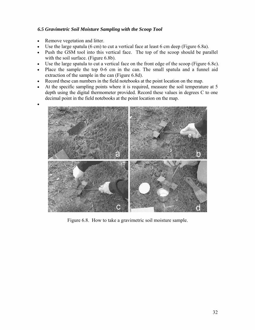
6.5 Gravimetric Soil Moisture Sampling with the Scoop Tool • Remove vegetation and litter. • Use the large spatula (6 cm) to cut a vertical face at least 6 cm deep (Figure 6.8a). • Push the GSM tool into this vertical face. The top of the scoop should be parallel

with the soil surface. (Figure 6.8b). • Use the large spatula to cut a vertical face on the front edge of the scoop (Figure 6.8c). • Place the sample the top 0-6 cm in the can. The small spatula and a funnel aid

extraction of the sample in the can (Figure 6.8d). • Record these can numbers in the field notebooks at the point location on the map. • At the specific sampling points where it is required, measure the soil temperature at 5

depth using the digital thermometer provided. Record these values in degrees C to one decimal point in the field notebooks at the point location on the map.

•

Figure 6.8. How to take a gravimetric soil moisture sample.

33

6.6 Gravimetric Soil Moisture Sample Processing All GSM samples are processed to obtain a wet and dry weight. It is the sampling teams responsibility to deliver the cans, fill out a sample set sheet, and record a wet weight at the field headquarters. A lab team will transport the samples and place them in the drying ovens. They will perform the removal of samples from the oven, dry weighing, and can cleaning. All gravimetric soil moisture (GSM) samples taken on one day will be collected from the field headquarters each afternoon. These samples will remain in the ovens until the following afternoon (approximately 24 hours). Wet Weight Procedure

1. Turn on balance. 2. Tare. 3. Obtain wet weight to two decimal places and record on sheet. 4. Process your samples in sample numeric order. 5. Place the CLOSED cans back in the box. Arrange them sequentially. 6. Place box and sheet in assigned locations.

Dry Weight Procedure

1. Each day obtain a balance reference weight on the wet weight balance and the dry weight balance.

2. Pick up all samples from field headquarters. 3. Turn off oven and remove samples for a single data sheet and place on

tray. 4. These samples will be hot. Wear the gloves provided 5. Turn on balance. 6. Tare. 7. Obtain dry weight to two decimal places and record on sheet. 8. Process your samples in sample numeric order. 9. All samples should remain in the oven for approximately 20-22 hours at

105oC. 10. Try to remove samples in the order they were put in. 11. Load new samples into oven. 12. Turn oven on. 13. Clean all cans that were removed from the ovens and place empty cans in

boxes. Check that can numbers are readable and replace any damaged or lost cans with spares.

14. Return the clean cans to the field HQ. 6.7 Soil Bulk Density and Surface Roughness All sites involved in gravimetric soil moisture sampling will be characterized for soil bulk density and surface roughness. The bulk density method being used is a volume

34

extraction technique that has been employed in most of the previous experiments and is especially appropriate for the surface layer. Three replications will be made at each field.

The Bulk Density Apparatus - The Bulk Density Apparatus itself consists of a 12" diameter plexiglass ring with a 5" diameter hole in the center and three 3/4" holes around the perimeter. Foam is attached to the bottom of the plexiglass. The foam is 2 inches high and 1 1/2 inches thick. The foam is attached so that it follows the circle of the plexiglass. Other Materials Required for Operation:

Three 12" (or longer) threaded dowel rods and nuts are used to secure the apparatus to the ground.

A hammer or mallet is used to drive the securing rods into the ground. A bubble level is used to insure the surface of the apparatus is horizontal to the

ground. A trowel is used to break up the soil. An ice cream scoop is used to remove the soil from the hole. Oven-safe bags are used to hold the soil as it is removed from the ground. The

soil is left in the bag when it is dried in the oven. Water is used to determine the volume of the hole. A plastic jug is used to carry the water to the site. One-gallon plastic storage bags are used as liners for the hole and to hold the

water. A 1000 ml graduated cylinder is used to determine the volume of the water.

Plastic is best because glass can be easily broken in the field. A turkey baster is used to transfer small amounts of water. A hook-gauge is used to insure water fills the apparatus to the same level each

time.

Selecting and Preparing an Appropriate Site -

1. Select a site. An ideal site to conduct a bulk density experiment is: relatively flat, does not include any large (>2 cm) rocks or roots in the actual area that will be tested and has soil that has not been disturbed.

2. Ready the site for the test. Remove all vegetation, large (>2 cm) rocks and other debris from the surface prior to beginning the test. Remove little or no soil when removing the debris.

35

Figure 6.9. How to take a bulk density sample Bulk Density Procedure - Securing the Apparatus to the Ground

1. Place the apparatus foam-side-down on the ground. 2. Place the three securing rods in the 3/4" holes of the apparatus. 3. Drive each dowel into the ground until they do not move easily vertically

or horizontally. (Figure 6.9a) Leveling the Apparatus Horizontally to the Ground

1. Tighten each of the bolts until the apparatus appears level and the foam is compressed to a height of 1" to 1 1/2".

2. Place the bubble level on the surface of the apparatus and tighten or loosen the bolts in order to make the surface level. Place the level in at least three directions and on three different areas of the surface of the apparatus.

Determining the Volume from the Ground to the Hook Gauge

1. Pour exactly one liter of water into the graduated cylinder. 2. Pour some of the water into a plastic storage bag. 3. Hold the plastic bag so that the water goes to one of the lower corners of

the bag.

36

4. Place the corner of the bag into the hole. Slowly lower the bag into the hole allowing the bag and the water to snugly fill all of the crevasses.

5. Slightly raise and lower the bag in order to eliminate as many air pockets as possible.

6. Lay the remainder of the bag around the hole. 7. Place the hook-gauge on the notches on the surface of the apparatus. 8. Add water to the bag until the surface of the water is just touching the

bottom of the hook on the hook-gauge. A turkey-baster works very well to add and subtract small volumes of water. Be sure not to leave any water remaining in the turkey-baster. (Figure 6.9b)

9. Place the graduated cylinder on a flat surface. Read the cylinder from eye-level. The proper volume is at the bottom of the meniscus. Read the volume of the water remaining in the graduated cylinder. Record this volume. Subtract the remaining volume from the original 1000 ml to find the volume from the ground surface to the hook-gauge.

10. Carefully transfer the water from the bag to the graduated cylinder. Hold the top of the bag shut, except for two inches at either end. Then use the open end as a spout. (It is best to reuse water, especially when doing multiple tests in the field.)

Loosening the Soil and Digging the Hole

1. Label the oven-safe bag with the date and test number and other pertinent information using a permanent marker.

2. Loosen the soil. The hole should be approximately six cm deep and should have vertical sides and a flat bottom. An ice cream scoop is helpful to scrape the bottom of the hole so that it is flat. (The hole should be a cylinder: with surface area the size of the hole of the apparatus and depth of six cm.)

3. Remove the soil from the ground and very carefully place it in the oven-safe bag. (Be careful to lose as little soil as possible.) (Figure 6.9c and d)

4. Continue to remove the soil until the hole fits the qualifications. 5. Loosely tie the bag so that no soil is lost in transportation.

Finding the Volume of the Hole

1. Determine the volume from the bottom of the hole to the hook-gauge as described in Determining the Volume from the Ground to the Hook-Gauge. Record this volume. Reusing the water from the prior measurement presents no potential problems and is necessary when performing numerous experiments in the field.

2. Subtract the volume of the first measurement from the second volume measurement. The answer is the volume of the hole.

Calculating the Bulk Density of the Sample

1. Weigh the sample, and subtract the tare weight of the bag. Record the weight.

37

2. Dry the soil in an oven at 105°C for at least 24 hours. 3. Reweigh the sample, and subtract the tare weight of the bag. Record the

weight. 4. Divide the dry weight of the sample by the volume of the hole. The result

is the bulk density of the sample. Potential Problems and Solutions After I started digging I hit a large (>2 cm) rock. What should I do? The best solution is to start over in another location. Also, you can remove the rock from the soil and subtract the volume of the rock from the total volume of the water. You should never include a rock in the density of the soil. Rocks have significantly higher densities than soil and will invalidate the results. Roots, corncobs, ants and even mole holes will also invalidate the results. If you find any of these things the best thing to do is start the test again at another site. After I began digging the hole I noticed one of the dowels wasn’t the apparatus firmly in place. Do I have to start over? Unfortunately, if you have already started digging you do have to start the experiment again. Replacing the dirt to find the volume between the ground surface and the hook-gauge will give an inaccurate volume and thus an inaccurate soil density. I noticed that the bag holding the water has a small leak. Is there anything I can do? If the leak began after you had already found the volume, it is not necessary to start again. The volume is being measured in the graduated cylinder. If you have already removed the appropriate volume of water leaks in the bag, it will not affect the results of the test. However, if you noticed the leak before finding the volume, you will have to start again. Surface Roughness Surface roughness photographs will be obtained using the grid board approach. For grasses this should be performed after canopy and thatch removal. Four replications will be made at each site. Two photos are taken at each location, one with the board going North/South, the other with the board going East/West. For row crops, photos will be taken across (c) and along (a) the rows. The soil surface must be visible; therefore it may be necessary to remove plants, but do not damage more plants than you have to. Push the board into the soil surface so that there is no space between the board and the soil surface. Place a card with the site ID on the board and take a photo of the board and the soil surface in front of the board. (see figure 6.10) Surface roughness photos will be taken once during the experiment unless there is a change in the field conditions (plowing, planting, harvesting …).

38

Figure 6.10. Surface Roughness Photo 6.8 Soil Temperature Probes

Several different types of temperature probes may be used to measure soil temperature. These all have a metal rod, plastic top and digital readout. The version used will be the Max/Min Waterproof Digital Thermometer (Figure 6.11).

Figure 6.11. Temperature Probe with Handle/Cover To Operate:

1. Press On/Off to switch on 2. Verify that the measurement is in Celsius and that the probe is not set to Max or

Min 3. Probed into 1 cm of soil at the desired location. 4. Wait for reading to stabilize, and then record the number in the field book. 5. Push the probe to a depth of 5 cm, let it stabilize and record data.

39

6. Push Probe to a depth of 10 cm, let it stabilize and record data. 7. Turn off probe and cover. If necessary the cover can be placed on the top of the probe and used as a handle, but do not force the probe into the ground with undue force, as the probe may break. Normal operation of the probe is simple, but please make sure that neither Max nor Min appear on the LCD. This is a different mode of operation and will not be used for this experiment. 6.9 Hydra Probe Soil Moisture Installations Figure 6.12 shows a close up of the Hydra probe. As with the installation of any soil moisture measuring instrument, there are two prime considerations: the location the probe is to be installed at, and the installation technique.

Figure 6.12. The Hydra probe used at the tower locations. Selecting a Location for the HP • The probe installation site should be chosen carefully so that the measured soil

parameters are "characteristic" of the site. • Care should be taken that the instrument settles into position before any

measurements are considered quality controlled. • Make sure that the site will be out of foot traffic and is carefully marked and flagged. Installation of the HP • The installation technique aims to minimize disruption to the site as much as possible

so that the probe measurement reflects the “undisturbed site” as much as possible.

40

o Dig an access hole. This should be as small as possible. o After digging the access hole, a section of the hole wall should be made

relatively flat. A spatula works well for this. o The probe should then be carefully inserted into the prepared hole section.

The probe should be placed into the soil without any side to side motion which will result in soil compression and air gaps between the tines and subsequent measurement inaccuracies. The center of the probe head should be at a depth of 5 cm. This will be give a sensing depth of 3-7 cm which will assure a stable signal, less sensitive to surface activity.

o After placing the probe in the soil, the access hole should be refilled. o For a near soil surface installation, one should avoid routing the cable

from the probe head directly to the surface. A horizontal cable run of 20 cm between the probe head and the beginning of a vertical cable orientation in near soil surface installations is recommended. Furthermore, sinking the wire deeper than the installation depth is a good method of insuring that the wire will not act as a surface water pathway.

Other general comments are below.

o Avoid putting undue mechanical stress on the probe. o Do not allow the tines to be bent as this will distort the probe data o Pulling on the cable to remove the probe from soil is not recommended. o Moderate scratches or nicks to the stainless steel tines or the PVC probe

head housing will not affect the probe's performance. 6.10 Vegetation Sampling The protocols used in past experiments have been adapted for this experiment Parameters • Photographs • Green and dry biomass • Surface reflectance • Leaf area (LAI) Vegetation sampling will be conducted on all of the soil moisture sampling fields. Three representative locations within each field will be sampled during the course of the study to quantify the full range of vegetative cover. An effort will be made to co-locate these sampling locations with the soil moisture sampling points. GPS coordinates of each location within a field will be recorded. Vegetative sampling is intended to estimate the average site conditions, and data are not intended for footprint averaging. Each field will be sampled once or twice during the growing season. If rapid growth is expected in particular fields, the frequency can be increased. Sampling locations will be selected to provide a representative sample from that area of the field. For grasses, weeds, winter wheat and other non-row crops, all vegetation

41

within a 0.44 m by 0.44 m area at a location will be removed. A folding wooden yardstick will be used to define the area. (see Figure 6.13)

Figure 6.13. Vegetation Sampling Frame

Data Recording Data will be recorded onto the sampling sheet illustrated in Figure 6.14. Data sheets will be maintained as part of the permanent experimental record to verify the data once it is entered into the computer.

Vegetative Sampling

Date: 06/05/2007 Time: 13:47 Observers: Lynn, Iva, Crop: Pasture Sample ID

Stand Height (cm)

Row Direction

Row Spacing (cm)

Stand Density

Green Biomass (g)

Dry Biomass (g)

A04-A 75 na na na 112.8 63.3 A04-B 66 na na na 96.2

Figure 6.14. Example of the vegetation sampling data sheet

6.10.1 Digital Photographs of Vegetation

42

Photographs will be taken of plot area at the time of sampling. These will be collected with a digital camera. A marker board will be used to mark the plot, field location, and date. Photographs will be collected at an oblique angle (30-45º from horizontal) and at nadir at a height of a minimum of 1 m above the canopy. Cameras will be fixed to a telescoping pole to allow positioning above the canopy and a remote trigger to collect data. Three photos will be taken in each plot in this order; marker board, oblique, and nadir. 6.10.2 Green and Dry Biomass To measure biomass a plant will be cut at the ground surface from each sampling row. The five plants for the sampling site will be placed into a plastic bag with a label for the sampling site. A separate tag with the sampling site id will be placed into the bag as additional insurance against damaged labels. These plants will be transported to the field facility for separation of the plant material into stalks and leaves for corn and stems and leaves for soybean. Corn plants can be separated into leaves and stalks in the field for easier transport to the laboratory. These plant parts will be placed into a bag for drying and marked with sample site id. Green biomass will be measured for both components (stalks or stems and leaves) by weighing the sample immediately after separation of the components. If the biomass has excess of moisture on the leaves and stalks this will be removed by blotting with a paper towel prior to weighing. Dry biomass will be determined after drying the plant components in ovens at 75C for 48 hours.

6.10.3 Ground Surface Reflectance Surface reflectance data is valuable in developing methods to estimate the vegetation water content and other canopy variables. Observations made concurrent with biomass sampling provide the essential information needed for larger scale mapping with satellite observations. In addition, reflectance measurements made concurrent with satellite overpasses allow the validation of reflectance estimates based upon correction algorithms. We are using instruments developed by CROPSCAN (http://www.cropscan.com). Other instruments may be also be used if available. Most hand-held radiometers, which are used to measure soil and plant reflectance in the field, have one detector that must be calibrated frequently for changing amounts of sunlight. Dual-detector instrument designs measure the amount of sunlight and the reflected light simultaneously; thus, fewer calibrations are required and data may be acquired rapidly. The CROPSCAN Multispectral Radiometer (MSR) is an inexpensive instrument that has up-and-down-looking detectors and the ability to measure sunlight at different wavelengths. The basic instrument is shown in Figure 6.15.

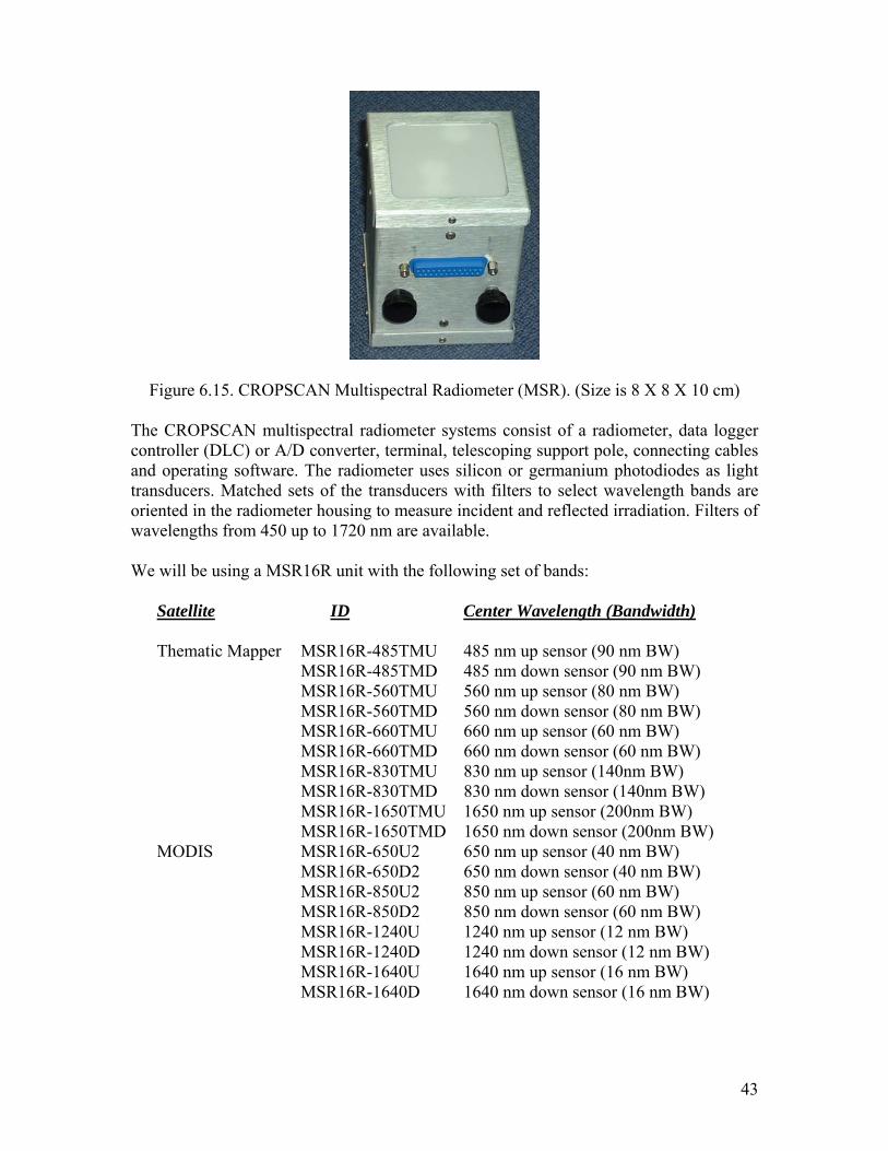
43

Figure 6.15. CROPSCAN Multispectral Radiometer (MSR). (Size is 8 X 8 X 10 cm) The CROPSCAN multispectral radiometer systems consist of a radiometer, data logger controller (DLC) or A/D converter, terminal, telescoping support pole, connecting cables and operating software. The radiometer uses silicon or germanium photodiodes as light transducers. Matched sets of the transducers with filters to select wavelength bands are oriented in the radiometer housing to measure incident and reflected irradiation. Filters of wavelengths from 450 up to 1720 nm are available. We will be using a MSR16R unit with the following set of bands:

Satellite ID Center Wavelength (Bandwidth) Thematic Mapper MSR16R-485TMU 485 nm up sensor (90 nm BW) MSR16R-485TMD 485 nm down sensor (90 nm BW) MSR16R-560TMU 560 nm up sensor (80 nm BW) MSR16R-560TMD 560 nm down sensor (80 nm BW) MSR16R-660TMU 660 nm up sensor (60 nm BW) MSR16R-660TMD 660 nm down sensor (60 nm BW) MSR16R-830TMU 830 nm up sensor (140nm BW) MSR16R-830TMD 830 nm down sensor (140nm BW) MSR16R-1650TMU 1650 nm up sensor (200nm BW) MSR16R-1650TMD 1650 nm down sensor (200nm BW) MODIS MSR16R-650U2 650 nm up sensor (40 nm BW) MSR16R-650D2 650 nm down sensor (40 nm BW) MSR16R-850U2 850 nm up sensor (60 nm BW) MSR16R-850D2 850 nm down sensor (60 nm BW) MSR16R-1240U 1240 nm up sensor (12 nm BW) MSR16R-1240D 1240 nm down sensor (12 nm BW) MSR16R-1640U 1640 nm up sensor (16 nm BW) MSR16R-1640D 1640 nm down sensor (16 nm BW)

44

These bands provide data for selected channels of the Landsat Thematic Mapper and MODIS instruments. Channels were chosen to provide NDVI as well as a variety of vegetation water content indices under consideration. In the field the radiometer is held level by the support pole above the crop canopy. The diameter of the field of view is one half of the height of the radiometer above the canopy. It is assumed that the irradiance flux density incident on the top of the radiometer (upward facing side) is identical to the flux density incident on the target surface. The data acquisition program included with the system facilitates digitizing the voltages and recording percent reflectance for each of the selected wavelengths. The program also allows for averaging multiple samples. Ancillary data such as plot number, time, level of incident radiation and temperature within the radiometer may be recorded with each scan.

Each scan, triggered by a manual switch or by pressing the space key on a terminal or PC, takes about 2 to 4 seconds. An audible beep indicates the beginning of a scan, two beeps indicate the end of scan and 3 beeps indicate the data is recorded in RAM. Data recorded in the RAM file are identified by location, experiment number and date.

The design of the radiometer allows for near simultaneous inputs of voltages representing incident as well as reflected irradiation. This feature permits accurate measurement of reflectance from crop canopies when sun angles or light conditions are less than ideal. Useful measurements of percent reflectance may even be obtained during cloudy conditions. This is a very useful feature, especially when traveling to a remote research site only to find the sun obscured by clouds. Three methods of calibration are supported for the MSR16R systems: 2-point Up/Down - Uses a diffusing opal glass (included), alternately held over the up and down sensors facing the same incident irradiation to calibrate the up and down sensors relative to each other (http://www.cropscan.com/2ptupdn.html).

Advantages: • Quick and easy. • Less equipment required. • Radiometer may then be used in cloudy or less than ideal sunlight conditions. • Recalibration required only a couple times per season. • Assumed radiometer is to be used where radiance flux density is the same

between that striking the top surface of the radiometer and that striking the target area, as outside in direct sunlight.

White Standard Up & Down - Uses a white card with known spectral reflectance to calibrate the up and down sensors relative to each other.

Advantages: • Provides a more Lambertian reflective surface for calibrating the longer

wavelength (above about 1200 nm) down sensors than does the opal glass diffuser of the 2-point method.

• Radiometer may then be used in cloudy or less than ideal sunlight conditions. • Recalibration required only a couple times per season.

45

• Assumed radiometer is to be used where radiance flux density is the same between that striking the top surface of the radiometer and that striking the target area, as outside in direct sunlight.

White Standard Down Only - Uses a white card with known spectral reflectance with

which to compare down sensor readings. Advantages: • Only down sensors required, saving cost of purchasing up sensors. • Best method for radiometer use in greenhouse, under forest canopy or whenever

irradiance flux density is different between that striking the top of the radiometer and that striking the target area.

Disadvantages: • White card must be carried in field and recalibration readings must be taken

periodically to compensate for sun angle changes. • Less convenient and takes time away from field readings. Readings cannot be made in cloudy or less than ideal sunlight conditions, because of likely irradiance change from time of white card reading to time of sample area reading.

There are six major items you need in the field -

• MSR16 (radiometer itself) • Data Logger Controller & Cable Adapter Box (carried in the shoulder pack,

earphones are to hear beeps) (Figure 6.16) • CT100 (hand terminal, connected to the DLC with a serial cable) (Figure 6.17) • Calibration stand and opal glass plate • Memory cards • Extension pole (with spirit level adjusted so that the top surface of the radiometer

and the spirit level are par level)

Figure 6.16. data logger controller & cable adapter box

46

Figure 6.17 CT100 hand terminal

Set Up – • Mount the radiometer pole bracket on the pole and attach the radiometer. • Mount the spirit level attachment to the pole at a convenient viewing position. • Lean the pole against a support and adjust the radiometer so that the top surface of

it is level • Adjust the spirit level to center the bubble (this will insure that the top surface of

the radiometer and the spirit level are par level) • Attach the 9ft cable MSR87C-9 to the radiometer and to the rear of the MSR

Cable Adapter Box (CAB) • Connect ribbon cables IOARC-6 and IODRC-6 from the front of the CAB to the

front of the Data Logger Controller (DLC) • Plug the cable CT9M9M-5 into the RS232 connectors of the CT100 and the DLC

(the DLC and CAB may now be placed in the shoulder pack for easy carrying) • Mount the CT100 on the pole at a convenient position • Adjust the radiometer to a suitable height over the target (the diameter of the field

of view is one half the height of the radiometer over the target)

Configure MSR – • Perform once at the beginning of the experiment, or if the system completely

loses power • Switch the CT100 power to on • Press ENTER 3 times to get into main menu • At Command * Press 2 then ENTER to get to the Reconfigure MSR menu • At Command * Press 1 then ENTER, input the correct date, Press ENTER • At Command * Press 2 then ENTER, input the correct time, Press ENTER • At Command * Press 3 then ENTER, input the number of sub samples/plot (5),

Press ENTER • At Command * Press 6 then ENTER, input a 2 or 3 character name for your

sampling location (ex OS for Oklahoma South), Press ENTER; input the latitude

47

for your location, Press ENTER; input the longitude for your location, Press ENTER

• At Command * Press 9 then ENTER, input the GMT difference, Press ENTER • At Command * Press M then ENTER until you return to the main menu

Calibration –

• We are using the 2-point up/down calibration method • Calibrate everyday before you begin to take readings • Switch the CT100 power to on • Press ENTER 3 times to get into main menu • At Command * Press 2 then ENTER to get to the Reconfigure MSR menu • At Command * Press 11 then ENTER to get to the Calibration menu • At Command * Press 3 then ENTER to get to the Recalibration menu • At Command * Press 2 then ENTER for the 2-point up/down calibration • Remove the radiometer from the pole bracket and place on the black side of the

calibration stand, point the top surface about 45° away from the sun, press SPACE to initiate the scan (1 beep indicates the start of the scan, 2 beeps indicate the end of the scan, and 3 beeps indicate the data was stored)

• Place the separate opal glass plate on top of the upper surface and press SPACE to initiate scan

• Turn the radiometer over and place it back in the calibration stand, cover it with the separate opal glass plate and press SPACE to initiate scan

• CT100 will acknowledge that the recalibration was stored • At Command * Press M then ENTER until you return to the main menu • Return the radiometer to the pole bracket • Store configuration onto the memory card

Memory Card Usage –

• Switch the CT100 power to on • Press ENTER 3 times to get into main menu • At Command * Press 7 then ENTER to get to the Memory Card Operations menu • Memory Card Operations menu is:

1. Display directory 2. Store data to memory card (use to save data in the field) 3. Load data from memory card (use first to download data from memory card) 4. Save program/configuration to card (use to save after calibrating) 5. Load program/configuration from card (use when DLC loses power) 6. Battery check M Main menu

• There are 2 memory cards, 64K for storing the program/configuration and 256 for storing data in the field

Taking Readings in the Field – • Switch the CT100 power to on • Press ENTER 3 times to get to MSR menu • Press ENTER to continue or M to return to the main menu • Enter beginning plot number, ENTER

48

• Enter the ending plot number, ENTER, record plot numbers and field ID in field notebook

• Adjust the radiometer to a suitable height (about 2 meters) over the target, point the radiometer towards the sun, center the bubble in the center of the spirit level and make sure that there are no shadows in the sampling area

• Do not take measurements if IRR < 300 • Initiate a scan by pushing SPACE, the message ‘scanning’ will appear on the

screen and a beep will be heard • When the scan is complete (about 2 seconds) ‘**’ will be displayed and 2 beeps

will be heard • Now, you can move to the next area • 3 Beeps will be heard when the data has been stored • Press SPACE to start next scan, R to repeat scan, P to repeat plot, S to

suspend/sleep, M to return to the MSR main menu, W to scan white standard, and D to scan Dark reading

• When you are done scanning at that field location, press M to return to the MSR main menu, then press 10 to put the DLC to sleep

• Switch the CT100 power off

Downloading Data – • Plug the cable RS9M9F-5 into the RS232 connectors on the front DLC and the

serial port of your PC • Start the CROPSCAN software on the PC • Choose RETRIEVE from the menu and press ENTER • Select your PC COM port and press ENTER • Enter your file name (MMDDFL.MV, where MM is month, DD is day, FL is first

and last initials of user and MV for raw millivolt data files) • After the data is downloaded, press Y then ENTER to clear the data from the

DLC Two types of sampling will be performed.

Vegetation Water Content Sampling Location:

Reflectance data will be collected for each vegetation sampling location (Figure 6.17) just prior to removal using the following sampling scheme. Making sure that the radiometer is well above the plant canopy; take a reading every meter for 5 meters. Repeat, for a total of 5 replications located 1 meter or 1 row apart.

49

Figure 6.17 Vegetation sampling scheme 6.10.4 Leaf Area

Leaf area will be measured with a LAI-2000 (Figure 6.18). The LAI-2000 will be set to average 5 points into a single value so one observation is taken above the canopy and 4 below the canopy. For grasses and weeds and non-row crops, five sets of measurements (each set consisting of 1 above the canopy and 4 beneath the canopy) will be made. Measurements will be taken every meter on 5 meter transects. For row crops, the 4 beneath canopy measurements will be taken across a plant row (in row, ¼ row, ½ row and ¾ row). If the sun is shining, the observer needs to stand with their back to the sun and put a black lens cap that blocks ¼ of the sensor view in place and positioned so the sun and the observer are never in the view of the sensor. The observer should always note if the sun was obscured during the measurement, whether the sky is overcast or partly cloudy with the sun behind the clouds. If no shadows could be seen during the measurement, then the measurement is marked “shaded”, if shadows could be seen during the measurement then the measurement is marked “sunny”. Conditions should not change from cloudy to sunny or sunny to cloudy in the middle of measurements.

1 Meter/Row

Crop Scan • Sampling

Vegetation Sampling Point

5 Meters

1 Meter

50

Figure 6.18. The LAI-2000 Instrument

Operating the LAI-2000 -

Plug the sensor cord into the port labeled “X” and tighten the two screws. Place a black view-cap over the lens that blocks 1/4 of the sensor view; that 1/4 that

contains the operator. Place a piece of tape on the view cap and body of the sensor so if the cap comes loose it will not be lost.

Turn on the logger with the “ON” key (The unit is turned off by pressing “FCT”, "0",

"9".) Clear the memory of the logger -

Press “FILE” Use “↑” to place “Clear Ram” on the top line of display Press “ENTER” Press “↑” to change “NO” to “YES” Press “ENTER”

General items –

When changing something on the display, get desired menu item on the top line of display and then it can be edited.

Use the “↑” and “↓” to move items through the menu and the “ENTER” key usually causes the item to be entered into the logger.

When entering letters, look for the desired letter on the keys and if they are on the lower part of the key just press the key for the letter; if the desired letter is on the upper part of the key then press the “↑” and then the key to get that letter.

Press “BREAK” anytime to return to the monitor display that contains time, file number or sensor readings on one of the five rings that are sensed by the LAI-2000.

Do not take data with the LAI-2000 if the sensor outputs are less than 1.0 for readings above the canopy.

51

To Begin - Press “SETUP”

Use “↑” to get “XCAL” on the top line of the display and press “ENTER” Following XS/N is the serial number of the sensor unit, enter appropriate number Check or put appropriate cal numbers from LICOR cal sheet into the 5 entries. Final press of “ENTER” returns you to “XCAL”

Use “↑” to get to “RESOLUTION” Set it to “HIGH”

Use “↑” to get to “CLOCK” Update the clock (set to local time using 24 hr format)

Press “OPER”

Use “↑” to get “SET OP MODE” on top line of display Choose “MODE=1 SENSOR X”

Enter “↑”, “↓”, “↓”, “↓”, “↓” in “SEQ” Enter "1" in “REPS”

Use “↑” to get to “SET PROMPTS” Put “SITE” in first prompt Put “LOC” in second prompt

Use “↑” to get to “BAD READING” Choose "A/B=1"

Press “BREAK” Display will contain the two monitor lines

Use “↑” and “↓” to control what is displayed on the top line in the monitor mode, time, file number or sensor ring output 1 through 5 for the X sensor. (If FI is selected, then the file number is displayed)

Use the “→” and “←” to control what is displayed on the bottom line of the monitor mode, time, file number or sensor ring output 1 through 5 for the X sensor. (If X2 is selected, then ring #2 output is displayed)

Press “LOG” to begin collecting data

Type in the response to the first prompt (if “ENTER” is pressed the same entry is kept in response to the prompt).

Type in the response to the second prompt (if “ENTER” is pressed the same entry is kept in response to the prompt).

Place the sensor head in the appropriate position above the canopy, level the sensor and press the black log button on the handle of the sensor (a beep will be heard when the black button is pushed). Hold the sensor level until the second beep is heard.

For Row crops – 1. Place the sensor head in the appropriate position above the canopy, level

the sensor and press the black log button on the handle of the sensor (a

52

beep will be heard when the black button is pushed). Hold the sensor level until the second beep is heard.

2. Place the sensor below the canopy in the row of plants, level the sensor and press the black log button on the sensor handle and keep level until the second beep.

3. Place the sensor one-quarter (1/4) of the way across the row and record data again.

4. Place the sensor one-half (1/2) of the way across the row and record data again.

5. Place the sensor three-quarters (3/4) of the way across the row and record data again. Repeat steps 1-5 so that you have a total of 5 sets of measurements.

For Other Types of Vegetation – 1. At your starting spot, place the sensor head in the appropriate position

above the canopy, level the sensor and press the black log button on the handle of the sensor (a beep will be heard when the black button is pushed). Hold the sensor level until the second beep is heard.

2. Place the sensor below the plant canopy in the same place level the sensor and press the black log button on the sensor handle and keep level until the second beep.

3. Repeat step 2 every meter, for a total of 1 up and 4 down measurements. 4. Repeat for a total of 5 transects.

The logger will compute LAI and other values automatically. Using the “↑” you can

view the value of the LAI. NOTE: You will record the “SITE” and “LOC” along with the LAI value on a

data sheet. The LAI-2000 is now ready for measuring the LAI at another location. Begin by

pressing “LOG” twice. The file number will automatically increment. When data collection is complete, turn off the logger by pressing “FCT”, "0", "9". The data will be dumped onto a laptop back at the Field Headquarters. Downloading LAI-2000 files to a PC Using HyperTerminal - Before beginning use functions 21 (memory status) and 27 (view) to determine which files you want to download. Make a note of their numbers.

1) Connect wire from LAI-2000 (25pin) to PC port (9 pin).

2) Run HyperTerminal on the PC (Start | Programs | Accessories | Communications |

HyperTerminal | LAI2000.ht)

53

3) On the LAI-2000, go to function 31 (config i/o) and configure I/O options. Baud=4800, data bits=8, parity=none, xon/xoff=no.

4) On the LAI-2000, go to function 33 (set format) and setup format options. First we

use Spdsheet and take the default for FMT. 5) In HyperTerminal go to Transfer | Capture text. Choose a path and filename

(LAIMMDDFL.SPR, where MM is month, DD is day, FL is first and last initials of user and SPR for spreadsheet data files) to store the LAI data. Hit Start. HyperTerminal is now waiting to receive data from the LAI-2000.

6) On the LAI-2000, go to function 32 (print) and print the files. ‘Print’ means send

them to the PC. You will be asked which file sequence you want. Eg. Print files from: 1 thru: 25 will print all files numbered 1-25. Others will not be downloaded.

7) Once you hit enter in function 32, lines of text data will be sent to HyperTerminal.

The LAI-2000 readout will say ‘Printing file 1, 2, etc’. Check the window in HyperTerminal to ensure the data is flowing to the PC. This may take a few minutes, wait until all the desired files have been sent.

8) In HyperTerminal go to Transfer | Capture text | Stop. 9) On the LAI-2000, go to function 33 (set format) and setup format options. Now

set to Standard, Print Obs = yes 10) In HyperTerminal go to Transfer | Capture text Choose a path and filename

(LAIMMDDFL.STD, where MM is month, DD is day, FL is first and last initials of user and STD for standard data files) to store the LAI data. Hit Start. HyperTerminal is now waiting to receive data from the LAI-2000.

11) On the LAI-2000, go to function 32 (print) and print the files. ‘Print’ means send

them to the PC. You will be asked which file sequence you want. Eg. Print files from: 1 thru: 25 will print all files numbered 1-25. Others will not be downloaded.

12) In HyperTerminal go to Transfer | Capture text | Stop. 13) Using a text editor (like notepad) on the PC, open and check that all the LAI data

has been stored in the text file specified in step 3. Make a back up of this file. Once you’re sure the LAI values look reasonable and are stored in a text file on the PC, use function 22 on the LAI-2000 to delete files on the LAI-2000 and free up its storage space.

Note: The above instructions assume that HyperTerminal has been configured to

interface with the LAI-2000, i.e. the file LAI2k.ht exists. If not, follow these instructions to set it up.

54

1) Run HyperTerminal on the PC (Start | Programs | Accessories | Communications | HyperTerminal | Hypertrm

2) Pick a name for the connection and choose the icon you want. Whatever you pick

will appear as a choice in the HyperTerminal folder in the start menu later. Hit OK.

3) Connect using com1 or com2. Choose your com port, hit OK. Setup Port settings

as follows: Bits per second = 4800, Data Bits = 8, Parity = none, Stop bits = 1, Flow control = Hardware. Say OK.

4) Make sure the wire is connected to the LAI-2000 and the PC and proceed with step 3 in the download instructions above. When finished and leaving HyperTerminal you will be prompted to save this connection.

55

7 Logistics

7.1 Security/Access to Fields

Do not enter the field unless you have permission to enter. If questioned, politely identify yourself and explain that you are with the NASA/SMAP experiment. There may be cattle in the field, so always leave all gates as you found them, open or closed.

7.2 Safety

General Field Safety

There are a number of potential hazards in doing field work. The following page has some good suggestions. Common sense can avoid most problems. Remember to:

• When possible, work in teams of two • Carry a phone • Know where you are. All roads have street signs. Make a note of your closest

intersection. • Do not touch or approach any unidentified objects in the field. • Dress correctly; long pants, long sleeves, boots, hat • Use sunscreen. • Carry plenty of water for hydration.

56

Ticks

Ticks are flat, gray or brownish and about an eighth of an inch long. When they are filled with their victim's blood they can grow to be about a quarter of an inch around. If a tick bites you, you won't feel any pain. In fact you probably won't even know it until you find the tick clamped on tightly to your body. There may be some redness around the area, and in the case of a deer tick bite, the kind that carries Lyme Disease, a red "bulls-eye" may develop around the area. This pattern could spread over several inches of your body.

When you find a tick on you body, soak a cotton ball with alcohol and swab the tick. This will make it loosen its grip and fall off. Be patient, and don't try to pull the tick off. If you pull it off and it leaves its mouth-parts in you, you might develop an irritation around these remaining pieces of tick. You can also kill ticks on you by swabbing them with a drop of hot wax (ouch!) or fingernail polish. After you've removed the tick, wash the area with soap and water and swab it with an antiseptic such as iodine.

Ticks are very common outdoors during warm weather. When you are outdoors in fields and in the woods, wear long pants and boots. Also spray yourself before you go out with insect repellent containing DEET.

Drying Ovens

The temperature used for the soil drying ovens is 105oC. Touching the metal sample cans or the inside of the oven may result in burns. Use the safety gloves provided when placing cans in or removing cans from a hot oven. Vegetation drying is conducted at 70

oC with is less hazardous.

Driving

• Observe speed limits and try to keep the dust minimal (slow down) around houses. • Watch for loose gravel, sand, and farm animals • Do not leave car unlocked (theft) • Do not leave all windows sealed when car is unattended (heat buildup can break a

window)

Lightning

• Lightning can be a deadly force, watch the skies for sudden cloud development. • Do not leave your vehicle in a thunderstorm.

7.3 Local Contacts and Shipping

Tyson Ochsner Oklahoma State University Department of Plant and Soil Sciences 368 Agricultural Hall Stillwater, OK 74078-6028 1-405-744-3627

57

8. References Cosh, M.H., T.J. Jackson, R. Bindlish, J. Famiglietti, and D. Ryu, 2005, A comparison of an impedance probe for estimation of surface soil water content over large region. Journal of Hydrology, 311:49-58. Doraiswamy, P. C., J. L. Hatfield, T.J. Jackson, B. Akhmedov, J. Prueger, and A. Stern, 2004. Crop condition and yield simulations using Landsat and MODIS, Remote Sensing of Environment, 92: 548-559.