Embed Size (px)
Citation preview

Software Pipelining
VICKI H. ALLAN
Utah State University
REESE B. JONES
E,,ans and Sutherland, 650 Komas Drive, Salt Lake City, UT 84108
RANDALL M. LEE
DAKS, 3017 Taylor Aven ue, Ogden, UT 84405
STEPHEN J. ALLAN
Utah State Unlvers~ty
Utilizing parallelism at the instruction level is an important way to improve
performance. Because the time spent in loop execution dominates total execution time,
a large body of optimizations focuses on decreasing the time to execute each iteration.
Software pipelining is a technique that reforms the loop so that a faster execution rate
m reahzed. Iterations are executed in overlapped fashion to increase parallelism.
Let {ABC]n represent a 100P contaimng operations A, B, C that is executed n times.
Although the operations of a single iteration can be parallelized, more parallelism may
be achieved if the entire loop is considered rather than a single iteration. The software
pipelimng transformation utilizes the fact that a loop {ABC)’ is equivalent to
A{ BCA}n -1 BC. Although the operations contained in the loop do not change, the
operations are from different iterations of the original loop.
Various algorithms for software pipelimng exist. A comparison of the alternate
methods for software pipelining is presented. The relationships between the methods
are explored and possibilities for improvement highlighted.
Categories and Subject Descriptors: D. 1.3 {Programming Technique]: Concurrent
Programming; D.3.4 [Programming Languages]: Processors—compilers,
optzmzzatzon
General Terms: Algorithms, Languages
Additional Key Words and Phrases: InstructIon level parallelism, loop reconstruction,
optimization, software pipelining
Authors’ addresses: Vicki H. Allan and Stephen J. Allan, Department of Computer Science at Utah StateUniversity, Logan, UT 84322-4205; e-mail: [email protected]. Reese B. Jones, Evans and Sutherland.Randall M. Lee, DAKS.
Permission to make dugital/hard copy of part or all of this work for personal or classroom use m grantedwithout fee provided that copies are not made or distributed for profit or commercial advantage, thecopyright notice, the title of the publication and its date appear, and notice m given that copying is by
permission of ACM, Inc. To copy otherwise, to republish, to post on servers, or to redistribute to lists,requires prior specific permission and/or a fee.@ 1995 ACM 0360-0300/95/0900-0367 $03.50
ACM Computmg Surveys, Vol 27, No. 3, September 1995

368 “ V. H. Allan et al.
CONTENTS
[INTRODUCTION1 BACKGROLTND INFORMATION
1 1 ModelLng Rewurce Usage
12 The Data Dependence Graph13 Generating a Schedule
14 Imtlatlonlnterval15 Factor5.Affectl ngthe Inltmtlon Inter\al16 Methods of Computmgll1 7 Unrolhn gRcpllcatlon18 support forsoft\”Jre Plpellnlng
2 L1ODULO SCHEDULING
2 1 illodulo Scheduling lEI HlerarchlcalReduction
22 Path Algebra
23 Predicated Modulo Scbeduhn~24 Enhanced Modulo Scheduling
3 KERNEL RECOGNITION31 Perfect P]pehnlng
32 Petri Net Model
33 Vegdahl’s Te~hnlque4 ENHANCED PIPELINE SCHEDULING
41 Inst, uctlon Model42 (}lobal Code Motion With Renammg
and Forw aId Substltutlon43 P]pclln, ng the Loop
.4-4 Reducing Code Expansion
5 SUMMARY
5 1 Modulo Scheduling Algorithms
52 Perfect Plpehnmg
53 Petri Net Model
54 Vegdahl
55 Enhanced Plpehne Scheduhng
6 CONCLUSIONS AND FUTURE WORK
ACKNOWLEDGMENTS
REFERENCES
INTRODUCTION
Software pipelining is an excellentmethod for improving the parallelism inloops even when other methods fail.Emerging architectures often have sup-port for software pipelining.
There are many approaches for im-proving the execution time of an applica-tion program. One approach involvesimproving the speed of the processor,whereas another, termed parallel pro-cessing, involves using multiple process-ing units. Often both techniques are used.Parallel processing takes various forms,
including processors that are physicallydistributed, processors that are physi-cally close but asynchronous, and syn-chronous multiple processors (or multiplefunctional units). Fine grain or instruc-tion level parallelism deals with the uti-lization of synchronous parallelism at theoperation level. This paper presents anestablished technique for parallelizingloops. The variety of approaches to thiswell understood problem are fascinating.A number of techniques for softwarepipelining are compared and contrastedas to their ability to deal with necessarycomplications and their effectiveness inproducing quality results. This paperdeals not only with practical solutions forreal machines, but with stimulating ideasthat may enhance current thinking onthe problems. By examining both thepractical and the impractical approaches,it is hoped that the reader will gain afuller understanding of the problem andbe able to short-circuit new approachesthat may be prone to use previouslydiscarded techniques.
With the advent of parallel computers,there are several methods for creatingcode to take advantage of the power ofthe parallel machines, Some propose newlanguages that cause the user to re-design the algorithms to expose paral-lelism. Such languages may be exten-sions to existing languages or completelynew parallel languages. From a theoreti-cal perspective, forcing the user to re-design the algorithm is a superior choice.However, there will always be a need totake sequential code and parallelize it.Regular loops such as fcm loops lendthemselves to parallelization techniques,Many exciting results are available forparallelizing nested loops [Zima andChapman 1991]. Techniques such as loopdistribution, loop interchange, skewing,tiling, loop reversal, and loop bumpingare readily available [Wolfe 1990, 1989].However, when the dependence of a loopdo not permit vectorization or simultane-ous execution of iterations, other tech-niques are required. Software pipeliningrestructures loops so that code from vari-ous iterations are overlapped in time.
ACM Computmg Surveys, Vol 27, No 3, September 1995

This type of optimization does not un-leash massive amounts of parallelism,but creates a modest amount of paral-lelism. The utilization of fine grain paral-lelism is an important topic in machinesthat have many synchronous functionalunits. Machines such as horizontal mi-croengines, multiple RISC architectures,VLIW, and LIW can all benefit from theutilization of low level parallelism.
Software pipelining algorithms gener-ally fall into two major categories: mod-U1O scheduling and kernel recognitiontechniques. This paper compares andcontrasts a variety of techniques used toperform the software pipelining opti-mization. Section 1 introduces termscommon to many techniques. Section 2discusses modulo scheduling; specificinstances of modulo scheduling are item-ized. Section 2.1 discusses Lam’s itera-tive technique for finding a softwarepipeline, and in Section 2.2 a mathemati-cal foundation is effectively used to modelthe problem. In Section 2.3, hardwaresupport for modulo scheduling is dis-cussed. Section 2.4 extends the benefitsof predicated execution to machineswithout hardware support. The next sec-tions discuss the kernel recognition tech-niques. In Section 3.1, the method ofAiken and Nicolau is presented. Sec-tion 3.2 demonstrates the application ofPetri nets to the problem, and Section3.3 demonstrates the construction of anexhaustive technique. Section 4 intro-duces a completely different technique toaccommodate conditionals. The finalsections summarize the various contri-butions of the algorithms and suggestfuture work.
1. BACKGROUND INFORMATION
1.1 Modeling Resource Usage
Two operations conflict if they requirethe same resource. For example, if 01and Oz each need the floating point adder(and there is only one floating pointadder), the operations cannot executesimultaneously. Any condition that disal-lows the concurrent execution of two op-
Software Pipelining ● 369
erations can be modeled as a conflict.This is a fairly simple view of resources.A more general view uses the followingto categorize resource usage:
(1)
(2)
(3)
(4)
Homogeneous/Heterogeneous. Theresources are termed homogeneousif they are identical, hence the op-eration does not specify which re-source is needed, only that it needsone or more resources. Otherwisethe resources are termed heteroge-neous.
Specific/General. If resources areheterogeneous and duplicated, wesay the resource request is specificif the operation requests a specificresource rather than any one of agiven class. Otherwise we say theresource request is general.
Persistent/Nonpersistent. We say aresource request is persistent if oneor more resources are required af-ter the issue cycle.
Re.mdar/Irre.mdar. We sav a re -so&ce i-eque;t is regular -if it ispersistent, but the resource use issuch that only conflicts at the issuecycle need to be considered. Other-wise we say the request is irregu-lar.
A common model of resource usage
(heterogeneous, specific, persistent, regu-lar) indicates which resources are re-quired by each operation. The resourcereservation table proposed by some re-searchers models persistent irregular re-sources [Davidson 197 1; Tokoro et al.1977]. This is illustrated in Figure 1 inwhich the needed resources for a givenoperation are modeled as a table in whichthe rows represent time (relative to in-struction issue) and the columns repre-sent resources (adapted from Rau [ 1994]).For this reservation table, a series ofmultiplies or adds can proceed one afteranother, but an add cannot follow a mul-tiply by two cycles because the result buscannot be shared. This low-level model ofresource usage is extremely versatile inmodeling a variety of machine conflicts.
ACM Comput]ng Surveys, Vol 27, No 3, September 1995

370 “
Time
o
1
2
3 I
V. H. Allan et al.
x
Time
0
1
‘2
3
4
5
(a)
kQAw@%-1
I I. .
I v, , -. 1
I 1 1 1 1
Illlllllxl
(b)
Figure 1. Possible reservation tables for (a) pipelined add and (b) plpehned multiply.
1.2 The Data Dependence Graph
In deciding what operations can executetogether, it is important to know which
operations must follow other operations.We say a conflict exists if two operationscannot execute simultaneously, but itdoes not matter which one executes first.A dependence exists between two opera-tions if interchanging their order changesthe results. Dependence between opera-tions constrain what can be done in par-allel. A data dependence graph (DDG) isused to illustrate the must-follow rela-tionships between various operations. Letthe data dependence graph be repre-sented by DDG( N, A), where N is theset of all nodes (operations) and A is theset of all arcs (dependence). Each di-rected arc represents a must-follow rela-tionship between the incident nodes. TheDDGs for software pipelining algorithmscontain true dependence, antidepen-dences, and output dependence. Let 01and Oz be operations such that 01 pre-cedes Oz in the original code, Oz mustfollow 01 if any of the following condi-tions hold: (1) Oz is data dependent on01 if Oz reads data written by 01, (2) Ozis antidependent on 01 if Oz destroysdata required by O ~ [Banerjee et al.1979], or (3) Oz is output dependent on
O ~ if Oz writes to the same variable asdoes O1. The term dependence refers todata dependence, antidependences, andoutput dependence.
There is another reason that one oper-
ation must wait for another operation. Acontrol dependence exists between a andb if the execution of statement a deter-mines whether statement b is executed[Zima and Chapman 1991]. Thus al-though b is able to execute because allthe data is available, it may not executebecause it is not known whether it isneeded. A statement that executes whenit is not supposed to execute could changeinformation used in future computations.Because control dependence have somesimilarity with data dependence, theyare often modeled in the same way[Ferrante et al. 1987].
The dependence information is tradi-tionally represented as a DDG. Whenthere are several copies of an operation(representing the operation in various it-erations), several choices present them-selves. We can let a different node repre-sent each copy of an operation or we canlet one node represent all copies of anoperation. We use the latter method. Assuspected, this convention does makethe graph more complicated to read andrequires the arcs be annotated.
ACM Computmg Surveys. Vol 27, No 3, September 1995

Software Pipelining “ 371
for i
01: a[i] = a[i] + 1
02: b[i] = a[i] / 2 X1 ITERATIONS
(0,1) ~ 11: 1 1 l.. .
Iz: 2 2 2 .,.
2 L~ 13: 3 3 3,. ,
03: c[i] = b[i] + 3
b
(0,1)14: 4 4 4 . . .
04: d[i] = c[i]
3
(0,1)
4
(a) (b) (c)
Figure 2. (a) Loop body pseudo-code. (b) Data dependence graph. (c) Schedule.
Dependence arcs are categorized asfollows. A loop-independent arc repre-sents a must-follow relationship amongoperations of the same iteration. A loop-carried arc shows relationships betweenthe operations of different iterations.Loop-carried dependence may turn tra-ditional DDGs into cyclic graphs [Zimaand Chapman 1991]. (Obviously, depen-dence are not cyclic if operations fromeach iteration are represented distinctly.Cycles are caused due to the representa-tion of operations.)
1.3 Generating a Schedule
Consider the loop body of Figure 2(a).1Although each operation of an iterationdepends on the previous operation, asshown by the DDG of Figure 2(b), thereis no dependence between the variousiterations; the dependence are loop in-dependent. This type of loop is termed adoall loop as each iteration is given anappropriate loop control value and mayproceed in parallel [Kuck and Padua1979; Chandy and Kesselman 1991]. The
1 We use pseudo-code to represent the operations.Even though array accessing 1s not normally avail-able at the machine operation level, we use thishigh-level machine code to represent the depen-dence as it is more readable than RISC code orother appropriate choices. We are not implying ourtarget machme has such operations.
assignment of operations to a particulartime slot is termed a schedule. A sched-ule is a rectangular matrix of sets ofoperations in which the rows representtime and the columns represent itera-tions. Figure 2(c) indicates a possibleschedule in which all copies of operation1 can execute together. A set of opera-
tions that executes concurrently istermed an instruction. All copies of oper-ation 1 execute together in the firstinstruction. Similarly, all copies of opera-
tion 2 execute together in the second in-struction. Although it is not required that
all iterations proceed in lock step, it ispossible if sufficient functional units arepresent.
Doall loops often represent massiveparallelism and hence are relatively easyto schedule. A doacross loop is one inwhich some synchronization is necessarybetween operations of various iterations
[Wolfe 1989]. The loop of Figure 3(a) isan example of such a loop. Operation 01of one iteration must precede O ~ of thenext iteration because the a[ i ] used iscomputed in the previous iteration. Al-though a doall loop is not possible, someparallelism can be achieved between op-erations of various iterations. A do acrossloop allows parallelism between opera-tions of various loops when proper syn-chronization is provided.
ACM Computmg Surveys, Vol 27, No 3, September 1995

372 “ V. H. Allan et al.
for (i=l;ii=n;i++
)O~:a[i+l]=ai]+l
02: b[i] = a[i + 1] / 2
03: c[i] = b[i] + 3
04: d[i]=c[i]
(a)
T “[2]= a[I\$E&ATIONS~ b[l] = a[2]/2 a[3] = a[2] + 1>
M c[l] = b[l] + 3 b[2] = a[3]/2 a[4] = a[3] + 1
E d[I] = c[l] c[2] = b[2] + 3 b[3] = a[4]/2
d[2] = C[2]
1! l\
c3=b 3+3
(b) d3=c3
(1,1)
!
fliaw
(0,1)H H
cl=b l/3a3=a2+l
2 b[2]=a[3]/2
(0,1) a[4]=a[3j+lfor (i=l;li=n-3;i++)
3
/
d i]=c[i]
(0)1) c i+l]=b[i+l]+3
XGI=WK
(postlude)
(c) (d)
ITERATIONS
dif
II:
L
“[ ‘~;: “n ; z
MIA:E
432
15: 4 32
16: 43
IT: 4
(e)
Figure 3. (a) Loop body pseudo-code. (b) First threeiterations of unrolled loop (c) DDG (d) Representa-
tive code for prelude and new loop body (postludeomitted) plpehne prelude, kernel, and postlude. (e)Execution schedule of Iterations. Time ( mzn ) is ver-tical displacement. Iteration ( dtf) M horizontal dis-placement. In this example mm = 1 and ahf = 1,The slope ( min/dzf) of the schedule M then 1 whichis the length of the kernel.
Because software pipelining enforcesthe dependence between iterations, butrelaxes the need for one iteration to com-pletely finish before another begins, it isa useful fine grain loop optimizationtechnique for architectures that support
synchronous parallel execution. The idea
behind software pipelining is that the
body of a loop can be reformed so thatone iteration of the loop can start beforeprevious iterations finish executing, po-
tentially unveiling more parallelism. Nu-merous systems completely unroll the
body of the loop before scheduling to takeadvantage of parallelism between itera-
tions. Software pipelining achieves an ef-fect similar to unlimited loop unrolling.
Inasmuch as adjacent iterations are
overlapped in time, dependence betweenvarious operations must be identified. To
see the effect of the dependence in Fig-ure 3(a), it is often helpful to unroll a fewiterations as in Figure 3(b). Figure 3(c)
shows the DDG of the loop body. In this
example, all dependence are true depen-dence. The arcs 1 + 2, 2 + 3, and 3 + 4
are loop independent and the arc 1 + 1is a loop-carried dependence. The differ-
ence (in iteration number) between the
source operation and the target operationis denoted as the fh-st value of the pair
associated with each arc. Figure 4 showsa similar example in which the loop-
carried dependence is between iterations
that are two apart. With this less restric-tive constraint, the iterations are moreoverlapped.
It is common to associate a delay with
an arc, indicating that a specified num-ber of cycles must elapse between theincident operations. Such delay is used to
specify that some operations are multi-
cycle, such as a floating point multiply.An arc a + b is annotated with a min
time that is the time that must elapsebetween the time the first operation isexecuted and the time the second opera-tion is executed. Identical operationsfrom separate iterations may be associ-ated with distinct nodes. An alternativerepresentation of nodes lets one noderepresent the same operation from alliterations. Because operations of a loop
behave similarly in all iterations, this isa reasonable notation. However, a depen-dence from node a in the first iteration tob in the third iteration must be distin-
ACM Computmg Surveys, Vol 27, No 3, September 1995

for (i=l; i<=n; i++)
01: a[i+ 2] = a[i] + 1
02: b[i] = ah+ 2] / 2
03: c[i] = b~] + 3
04: dfi]=cfi]
(a)
ITERATIONS
I b[llW;;,:l;IT a[3 = a[l] + 1 a[4] = u[2] + 1
~ c[l] = b[l] + 3d[2] = C[2]
[d[l] = C[l] c[3] = b[3] + 3
d[3] = C[3]
!2,1)
1
(0,1)
2
(0,1)3
(0,1)4
(b)
(c)
ITERATIONS
difI 1
II:
12:
~13:
M 14:
E 15:
16:
17:
[“1 .1,
mi22”11
33 2 2“”1. .1
443 322’ 1.,1
44 3 3 2 J!
4433
(d) 44
Figure 4. (a) Loop body code. (b) First three itera-tions of unrolled loop (c) DDG. (d) Execution sched-
ule of iterations.
guished from a dependence between aand b of the same iteration. Thus inaddition to being annotated with mintime, each dependence is annotated withthe dif that is the difference in the itera-tions from which the operations come. Tocharacterize the dependence, a depen-dence arc, a + b, is annotated with a(dif, rein) dependence pair. The dif valueindicates the number of iterations the
Software Pipelining “ 373
dependence spans, termed the iterationdifference. If we use the convention thata m is the version of a from iteration m,then (a + b, dif, rein) indicates there isa dependence between am and b m+”’,V m. For loop-independent arcs, dif iszero. The minimum delay intuitively rep-resents the number of instructions thatan operation takes to complete. Moreprecisely, for a given value of rein, if amis placed in instruction t ( 1~), then b ~ + ~’ ~can be placed no earlier than It+,.,,,.
Table 1 shows examples of code thatcontain loop-carried dependence. For thecode shown, a precedes b in the loop.The loop control variable is i, y is anyvariable, m is an array, and x is anyexpression. For example, the first rowindicates that m is assigned a value twoiterations before it is used. Thus it is a
true dependence with a dif of 2.If each iteration of the loop in Figure
3(a) is scheduled without overlap, fourinstructions are required for each itera-tion as no two operations can be done inparallel (due to the dependence). How-ever, if we consider operations fromseveral iterations, there is a dramaticimprovement.2 In Figure 3(e) we assumefour operations can execute concurrentlyallowing all four operations (from fourdifferent iterations) to execute concur-rently in 11.
When operations from all iterations arescheduled simultaneously, operations arescheduled as early (in execution time) aspossible. However, if one had to store thecode from all iterations of the unrolledloop, it would be prohibitive as therewould be many copies of each operation.Thus one seeks to minimize the codeneeded to represent the improved sched-ule by locating a repeating pattern in thenewly formed schedule. The instructionsof a repeating pattern are called the ker-nel, 2?, of the pipeline. In this paper, weindicate a kernel by enclosing the opera-tions in a box as shown in Figure 3(e).
z Scheduling in a parallel environment is some-times called compaction as the schedule produced isshorter than the sequential version.
ACM Computmg Surveys, Vol. 27, No 3, September 1995

374 e V. H. Allanet al.
Tablel. Dependence Examples
Instruction DDG A 7’C
Label Instruction Arc Type Dif
m[i+2]=x
; y = m[i] a-b true 2
y=m[i +3]
: m[i] = x a~b anti 3
m[i] = x
: y=m[i–2] a-b true 2
y = m[i]
; m[i–3]=x a~b ant i 3
yzt a+b anti o; t=x+i b-+a true 1
t=x+i a-+b true o; y=t b~a anti 1
y=x+i
: if(x>2)y=t a~b output o
kITERATIONS
1
for i II: 1 1 1
O~:a[i]=i*t(0,1) T 12:
(1,1)2
I
0, : b[i] = U[Z] * b[i - 1] 2M Is: 3,4 2
03: c[i] = b[i]/n E 14: 3%4 2
04: d[i] = b[i] % n (0,1) 0,1) Is: 3,4
3 4
(a) (b) (c)
Figure 5. (a) Loop body code. (b) DDG, (c) Schedule.
The kernel 1s the loop body of the newloop. Because the work of one iteration isdivided into chunks and executed in par-allel with the work from other iterations,it is termed a pipeline.
There are numerous complications that
can arise in pipelining. In Figure 5(a), OSand Oi from the same iteration can beexecuted together as indicated by 3, 4 inthe schedule of Figure 5(c). Note thatthere is no loop-carried dependence be-
tween the various copies of O1. When
scheduling operations from successive it-erations as early as dependence allow
(termed greedy scheduling), as shown inFigure 5(c), O ~ is always scheduled inthe first time step Il. Thus the distance
between O ~ and the rest of the opera-tions increases in successive iterations. Acyclic pattern (such as those achievablein other examples) never forms. In theexample of Figure 6(b),3 a pattern does
ACM Computmg Surveys Vol 27, No 3, September 1995

Software Pipelining ● 375
~?
(0,1)
2 5
(0,1) 0,1)
@
(0,1)3
(a)
14:M
15:E
16:
17:
&:
ITERATIONS1
n21
3,5 2
4 3,5
41
2
3,5
4
(b)
11: 1ITERATIONS
12: 2 1
13: 3,5 5
~4:421
15: 3,4 2
116: 5 1,5
2IT: 3,4 2
3,5 18:3,4 1
Ig : 2,5
(c)
Figure 6. (a) DDG. (b) Schedule that forms a pattern. (c) Schedule that does not form a pattern,
emerge and is shown in the box. Notice itcontains two copies of every operation,The double-sized loop body is not a seri-ous problem as execution time is not af-fected, but code size does increase in thatthe new loop body is four instructions inlength. Note that delaying the executionof every operation to once every secondcycle would eliminate this problem.
In Figure 6(c) a random (nondetermin-istic) scheduling algorithm prohibits apattern from forming quickly. As can beseen, care is required when choosing ascheduling algorithm for use with soft-ware pipelining.
1.4 Initiation Interval
In Figure 3(e) a schedule is achieved inwhich an iteration of the new loop isstarted in every instruction. The delaybetween the initiation of iterations of thenew loop is called the initiation interval
(11) and is the length of 2. This delay isalso the slope of the schedule that isdefined to be min/dif. The new loop bodymust contain all the operations in theoriginal loop. When the new loop body isshortened, execution time is improved.
3 It is assumed that a maximum of three operationsmay be performed simultaneously, General re-source constraints are possible, but we assumehomogeneous functional units in this example forsimplicity of presentation.
This corresponds to minimizing the effec-tive initiation interval that is the aver-age time one iteration takes to complete.The effective initiation interval is(11/iteration_ct), where iteration-et is
the number of copies of each operation inthe loop W.
Figure 4(d) shows a schedule in whichtwo iterations can be executed in everytime cycle (assuming functional units areavailable to support the eight operations).The slope of this schedule is min/dif = ~.
Notice that this slope indicates how manytime cycles it takes to perform an itera-tion. Because two iterations can be exe-cuted in one cycle, the effective executiontime for one iteration is + time cycle.
Notice that because %’ does not start orfinish in exactly the same manner as theoriginal loop L, instruction sequences aand Q are required to respectively filland empty the pipeline. In Figure 3(d), aconsists of instructions 11, 12, and IS andis termed the prelude. Q consists of in-structions 15, 16, and IT and is termed
the postlude. If the earliest iteration rep-resented in the new loop body is iterationc, and the last iteration represented inthe new loop body is iteration d, thespan of the pipeline is d – c + 1. If Yspans n iterations, the prelude must startn — 1 iterations preparing for thepipeline to execute, and the postludemust finish n – 1 iterations from thepoint where the pipeline terminates.
ACM Computmg Surveys, Vol 27, No 3, September 1995
376 e V. H. Allan et al.
Hxx
(0,1)
~(!)x
x 5
(a’)
1
2
3,4
5
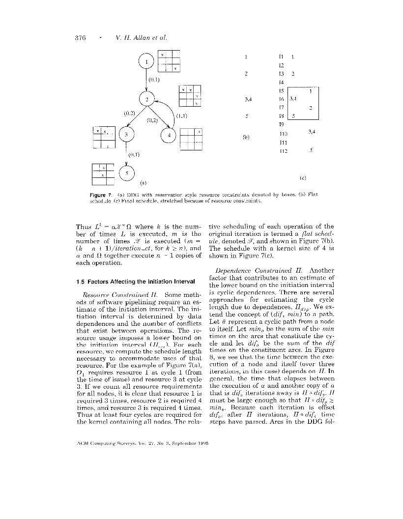
Figure 7. (a) DDG with reservation style resource constraints denoted
~chedule (c) Final schedule, stretched because of resource constraints
Thus Lk = c&?” Q where k is the num-ber of times L is executed, m is thenumber of times z is executed ( m =
(k – n + 1)/iteratio~z-et, for k > n), anda and Q together execute n – 1 copies ofeach operation.
1.5 Factors Affecting the Initiation Interval
Resource Constrained II. Some meth-ods of software pipelining require an es-timate of the initiation interval. The ini-tiation interval is determined by datadependence and the number of conflictsthat exist between operations. The re-source usage imposes a lower bound onthe initiation interval (11,,, ). For each
resource, we compute the schedule lengthnecessary to accommodate uses of thatresource. For the example of Figure 7(a),O ~ requires resource 1 at cycle 1 (fromthe time of issue) and resource 3 at cycle3. If we count all resource requirementsfor all nodes, it is clear that resource 1 isrequired 3 times, resource 2 is required 4times, and resource 3 is required 4 times.Thus at least four cycles are required forthe kernel containing all nodes. The rela-
11
1~
13
14
15
16
17
18
19
1
---11
3,’4
~
5
110 3,4
111
112 5
(c)
by boxes. (b) Flat
tive scheduling of each operation of theoriginal iteration is termed a flu t sched-ule, denoted :5, and shown in Figure 7(b).The schedule with a kernel size of 4 isshown in Figure 7(c).
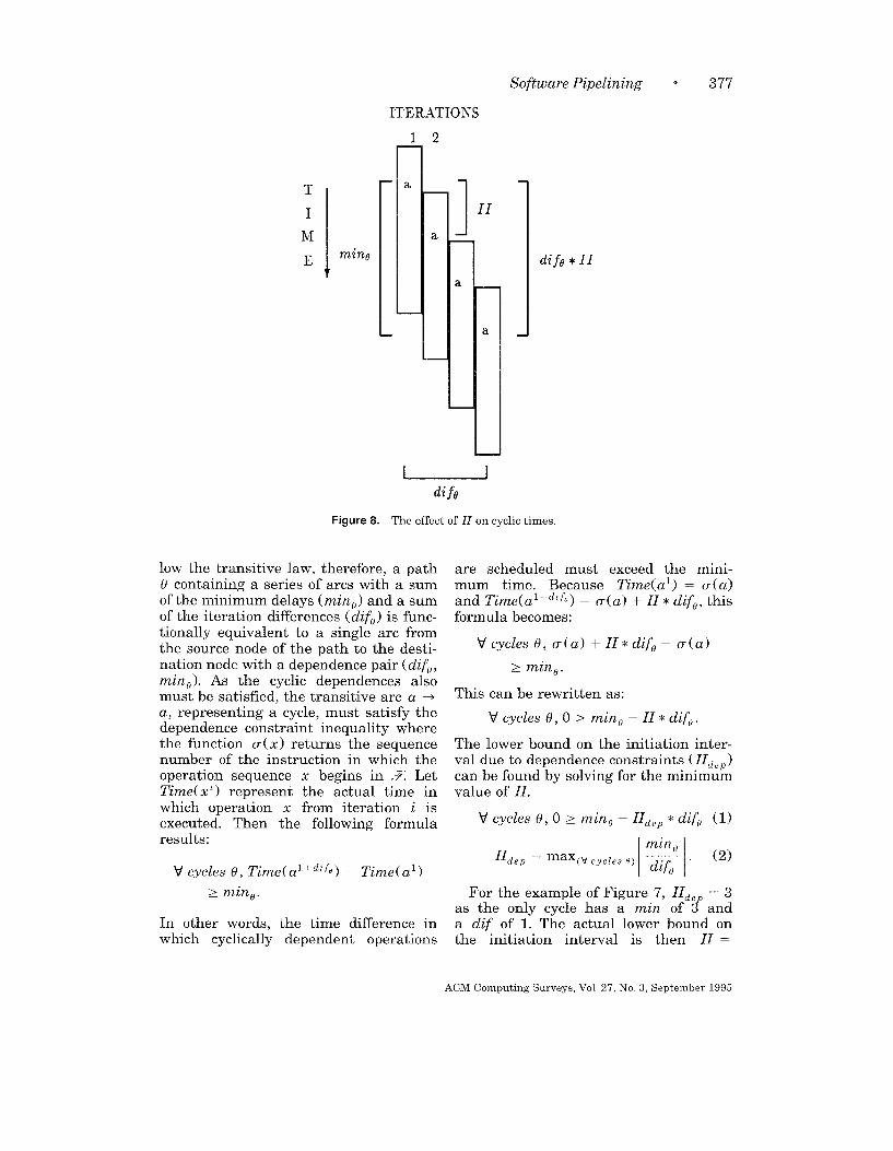
Dependence Constrained II. Anotherfactor that contributes to an estimate ofthe lower bound on the initiation intervalis cyclic dependence. There are severalapproaches for estimating the cyclelength due to dependence, ll~.P. We ex-tend the concept of (dif, min ) to a path.Let 0 represent a cyclic path from a nodeto itself. Let minfl be the sum of the mintimes on the arcs that constitute the cy-cle and let dife be the sum of the diftimes on the constituent arcs. In Figure8, we see that the time between the exe-cution of a node and itself (over threeiterations, in this case) depends on H. Ingeneral, the time that elapses betweenthe execution of a and another copy of athat is dif, iterations away is H ~ dife. II
must be large enough so that 11 * dife >mine. Because each iteration is offsetdzfti, after II iterations, II* dif~ timesteps have passed. Arcs in the DDG fol-
ACM Computmg Surveys, Vol 27, No 3. September 1995
Software Pipelining “ 377
ITERATIONS
T
I
M
Emine
t
1—
a
—
L--
2
—
a
—
1-1II
—
a
—
—
a
—
J
1dife *II
difo
Figure 8. The effect of 11 on cyclic times.
low the transitive law, therefore. a path are scheduled must exceed the mini-6 containing a series of arcs with a >umof the minimum delays (mine) and a sumof the iteration differences ( difo ) is func-tionally equivalent to a single arc fromthe source node of the path to the desti-nation node with a dependence pair ( dife,mine). As the cyclic dependence alsomust be satisfied, the transitive arc a ~a, representing a cycle, must satisfy thedependence constraint inequality wherethe function U(x) returns the sequencenumber of the instruction in which theoperation sequence x begins in Y; LetTime( x‘ ) represent the actual time inwhich operation x from iteration i isexecuted. Then the following formularesults:
‘d cycles 0, Time(al+d’ffl) – Time(al)
> mine.
In other words, the time difference inwhich cyclically dependent operations
mum time. Because Time(al) = u(a)and Time(al+d’f” ) = a(a) + H* dife, thisformula becomes:
‘d cycles 9, a(a) +II*difO – a(a)
This can be rewritten as:
V cycles 0, 0> mine – II* diffl.
The lower bound on the initiation inter-val due to dependence constraints ( IId,P )
can be found by solving for the minimumvalue of H.
b’ cycles 0, 0> mine – IId,P * difti (1)
[–1minflII~eP =
‘ax(v CYc’es0) difd “(2)
For the example of Figure 7, ll~.P = 3as the only cycle has a min of 3 anda dif of 1. The actual lower bound onthe initiation interval is then H =
ACM Computing Surveys, Vol 27, No 3, September 1995

378 ● V. H. Allan et al.
Iterations Iterations
T
I
M
E
difI-i1—
a
b
.
2
1
1J!’fa,b
a
b
—
(a)
{a+ b,d~f = l,min}
T
I
~a,b = rein– II* dif M
ninE
I11
-1
d,f
n
12
7
:
b
a
b
a
(b)
Figure 9. The effect of II on muumum times between nodes, Each rectangle represents the schedule of
one Iteration of the orlgmal loop. [a) Posltlve value for Ma ~, indicates a precedes b (b) A negatme valuefor Mu ~ indicates a follows b.
max( ll~pP, 11,,, ), which is 4 for this ex-ample. Any cycle having min /dif equalto II is termed a critical cycle.
1.6 Methods of Computing //
1.6.1 Enumeration of Cycles
One method of estimating II~,P simply
enumerates all the simple cycles [Matetiand Deo 1976; Tiernan 1970]. The maxi-mum ( min/ciif) for all cycles is then theH,,, [Dehnert et al. 1989].
1.6.2 Shortest Path Algorithm
Another method for estimating II~,P usestransitive closure of a graph. The transi-tive closure of a graph is a reachabilityrelationship. If the dependence con-straints are expressed as a function of II,a single calculation to compute the tran-sitive closure is sufficient. This symboliccomputation of closure allows the closureof the dependence constraints to be cal-culated independently of a particularvalue for II. The dependence constraint
between nodes in the closure is repre-sented by the set of distances4 by whichthe two nodes must be separated in Y– inorder to satisfy dependence. In the flatschedule, the distance, computed from asingle(dif, min ) dependence pair for an
arc a + b, is given by Ma, b = min –H Y dif. We would like to compute theminimum distance two nodes must beseparated, but as this information is de-pendent on H (which is a variable) onecannot simply take the maximum dis-tance for all paths between a and b. Asshown in Figure 9, we see that an arcfrom a to b with a di~ of 1 implies that b
must follow a (in the flat schedule) bymin — H time units. In general, an arc( ?2, + nj, dif, rein) is equivalent to thearc (n, ~ nj, O, min – dif * II), providedH is known. As shown in Figure 9(b),this new minimum value can be nega-tive. For example, Ml, ~ = – 3 indicates
4 This distance M referred to as the cost In transi-tive closure algorithms
ACM Computing Sumeys. Vol 27, No 3, September 1995

Software Pipelining “ 379
that n ~ can precede n, in the flat sched-ule by 3 time units. This computationgives the earliest time nJ can be placed
with respect to n ~.If there are two paths from a to b, one
having ( cZif, m in ) = (3, 8) and the otherhaving (cZif, rnin) = (1, 5), it is not evi-
dent which represents the stricter con-straint. In the first case, we have M,, ~ =8 – 3 II whereas in the second case wehave M, ~ = 5 – 1 ~ 11. If 11<2, the firstis larger. For example, if 11 = 1, 8 – 3 >
5 – 1. If H >2, the (dif, nlin) for thesecond arc represents the larger dis-tance. For example, when 11 == 2, 8 –3 ~~2<5 – 2. Thus both distances be-
tween a and b must be considered un-less one can be eliminated by discovering11 is sufficiently large. In the previousexample, if 11 is known to be at least 2
(due to the computation of lower bounds),then whenever (1, 5) is satisfied so is (3,$), and the latter constraint can be ig-nored. Computing the closure of the de-
pendence constraints is equivalent tofinding the longest path between eachpair of nodes in the strongly connectedcomponent. By Equation (l), we see cy-cles always have a zero or negative dis-tance. Therefore, by reversing the senseof all inequalities, one can use Floyd’sAll-Points Shortest Path Algorithm to
calculate the all-points longest path[Smith 1987].’
Let N be the set of nodes in the graph.The cost matrix C is defined as follows:entrY C, ~ contains the set of all depen-
dence information that influences the
longest path between i and j, that is, the( dif, min ) dependence pairs representingthe transitive closure of the dependencearcs between node i and node j. Initiallythe C,j set contains the ( dif, rnin) depen-
dence pairs of arcs in the strongly con-nected component. The closure of thedependence constraint is calculated as
5 Floyd’s original algorithm handles negative costsif all cycles have positive costs
follows :
‘dhEN’v’i~NVj~N
C,, = Ma.~Cost (C’,,, AddCost ( C,k , C,, )) .
The function AddCost creates an up-dated cost set by adding every de-pendence pair in the first set to everydependence pair in the second set, com-ponent-wise. The function MaxCost re-turns a set that is the union of the twosets with the redundant dependence pairsremoved. A cost is redundant if it is un-necessary because it provides no addi-tional constraints. Determining whetherone of (difl, rrzinl) or (difz, nainz ) is re-dundant involves two separate tests. Ifrninl – H*(difl) < minz – ll-(difz),then the distance associated with
( difz, mirzz ) is currently longer than thedistance associated with (difl, nzinl). Ifdifl > clifz, then for all larger values of
11, the distance of ( difz, nzin ~ ) remainslonger due to the fact that 11 has a nega-tive coefficient in the distance formula.
Formally, given a dependence pair
( difl, nzinl) and any other dependencepair ( difz, rninz ) in the distance set, then(difl, nzinl) is redundant if difl z difzand mini — nzinz < II * ( difl – difz ).From the previous example in whichpairl = (3, 8) and pairz = (1, 5), if weassume H = 2, pairl can be shown to beredundant as3>land8–5<2*(3–1).
For an initiation of H, the cost func-tion (cost 11(i, j)) gives the number of in-structions by which node j must follownode i in the flat schedule. The depen-dence constraint is defined as follows:
cost rr(i, j)
= ‘axfvf~,f,,~,)~c,,) lnin –IIY dif.
After the closure of the dependence con-straints is calculated, the dife and rnintivalues for all cycles 6 in the 13DG are
available to calculate 11,1,], (the minim-
um initiation interval due to depen-
dence constraints). This is similar to
computing the all-points longest path of
ACM Cornput]ng Surveys, V(,1 27, N,, 3, September 1995
380 “ V. H. Allan et al.
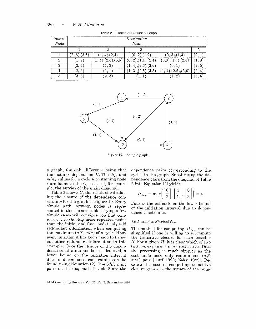
Table 2. Transltlve Closure of Graph
Source Destination
Node Node
, 1 . I . I . I .I I 1 I L I a I 4 1~1!
1 (2, 6),(3,6) (1, 4),(2,4) (o, 2),(1,2) (0, 3),(1,3) ‘ (o, 1)
2 (1,2) (1,4),(2,6),(3,6) (O, 2),(1,4),(2,4) (0,3),(1,5),(2,5) (1, 3)
3 (2. 4) (1. 2) (1. 4).(2.6).(3.6) (o, 1) (2, 5)
4 (2, 3) (1, 1) (1, 3),(2,5),(3,5) (1, 4),(2,6),(3,6) (2, 4)
5 (3, 5) (2, 3) (1, 1) (1, 2) (3, 6)
I I ,—, –, I ,–, —, I ,–, -,, \—, -,,\-,-,
(1, 2)
9
.
(o, 1)
(1, 1)
J
P
(o, 2)
3
Figure 10. Sample graph
a graph, the only difference being thatthe distance depends on II. The diffl andmine values for a cycle () containing node
i are found in the C,, cost set, for exam-ple, the entries of the main diagonal.
Table 2 shows C, the result of calculat-ing the closure of the dependence con-straints for the graph of Figure 10. Everysimple path between nodes is repre-sented in this closure table. Trying a fewsimple cases will convince you that com-plex cycles (having more repeated nodes
than the initial and final node) onlv add.redundant information when computingthe maximum ( dif, min ) of a cycle. How-ever, no attempt has been made to throwout other redundant information in thisexam~le. Once the closure of the de~en-dence’ constraints has been calculat~d, alower bound on the initiation intervaldue to dependence constraints can befound using Equation (2). The ( dif, rein)
pairs on the diagonal of Table 2 are the
(1,1)
dependence pairs corresponding to thecycles in the graph. Substituting the de-pendence pairs from the diagonal of Table2 into Equation (2) yields:
Four is the estimate on the lower boundof the initiation interval due to depen-dence constraints.
1.6.3 Iterat[ve Shortest Path
The method for computing II~,p can besimplified if one is willing to recomputethe transitive closure for each possibleII. For a given II, it is clear which of two( dif, m in} pairs is more restrictive. Thus
the processing is much simpler as the
cost table need only contain one (dif,
rnin) pair [Huff 1993; Zaky 1989]. Be-
cause the cost of computing transitive
closure grows as the square of the num-
ACM Computmg Surveys, Vol 27, No 3, September 1995

(O,l)j
Figure 11. Sample graph.
ber of values at a cost entry, this is asizable savings.
Path algebra is an attempt to formu-late the software pipelining problem inrigorous mathematical terms [Zaky1989]. Zaky constructs a matrix M thatindicates for each entry M,, ~ the mintime between the nodes i and j. Thisconstruction is simple in the event thatthe dif value between two nodes is zero.Assume a == n, and b = nj. If there is anarc (a ~ b, dif = O, rein), M, ~ = min.As is shown in Figure 9, we see that anarc (a ~ b, dif = 1, rein) implies than njmust follow n, by min – H time units.In general, an arc (n, ~ n], dif, rein)represents the distance min – dif * H.
This computation gives the earliest timenj can be placed with respect to n, in the
flat schedule. The drawback is that be-fore we are able to construct this matrix,we must estimate 11. The technique al-lows us to tell if the estimate for 11 islarge enough and iteratively try larger 11until an appropriate 11 is found.
Consider the graph of Figure 11. Foran estimate of 11 = 2, the matrix M isshown in Figure 12(a). Note that accord-ing to this matrix (for restrictions due topaths of length one), n~ and n4 can exe-cute together ( M2, ~ = O). Even thoughthere must be a min time of 2 betweenn~ of one iteration and n ~ from the nextas given by (n~ ~ n4, 1,2), the delay be-tween iterations (11 ) is two. Hence no
Software Pipelining “ 381
1 2 3 4 5 6 7
1 –cc 1 –w –m –co –cc –w
2 –cc –m –1 –cc –cc 1 –w
3 –w –W –co cl –cc –00 –m
4 –cc –cc -w -cc 1 –cc –co
5 –1 –w –cc –cc –cc –W –cc
6 –cc –00 –w –co -’m -cc 1
7 –cc –lx –m -cc –co –3 –co
[a) Original Matrix M
T
11 -m
2 –cc
3 –m
40
5 –cc
6 -m
7 –w
2
—w
–’x
—co
–cc
o
-m
–cc
lT-
12
101
2 –1 o
301
401
5 –1 o
6 –co –w
7 –00 –co
TT34.5
0 –m –cc
–w –1 –CO
–m –cm 1
–CO –m –cc
E(b) M2
?T345
001
–1 –1 o
001
0 0 1–1 –1 o
–@J]-co ]-co
—m –cc –cc
6
2
—cm
–cc
–m
–2
–w
7
—co
2
-m
–cc
-m
—cc
–2
t
67
23
12
23
23
12
–2 1–3 –2
(c) Closure
Figure 12. Closure computation.
further distance between nq and nL isrequired in the flat schedule:
Zaky defines a type of matrix multiplyoperation, termed path composition, suchthat M 2 = M 8 M represents the mini-mum time difference between nodes thatis required to satisfy paths of lengthtwo. For two vectors (al, az, a~, aq) and
(b,, bz, b,, b~), (al, az, a,, al) @ (b,, bz,b~, b4)=al@ bl@a2@b2@a~@b~@a4 @ b4. Notice that this is similar to aninner product. @ has precedence over Q.@ is addition, and Q is maximum.6 Forexample, to get M 2( 1, 6) we compose row
e It may seem strange that @ is addition, but the
notation was chosen to show the similarity betweenpath composition and inner product.
ACM Computmg Surveys, Vol 27, No 3, September 1995

382 . V. H. Allan et al.
1 of the preceding matrix with column 6as follows:
[–z, ~,-~, -x,
@J–z, l, –z,
=7nax( -=,2,
= 2.
Thus there is aedges (indicatedi%?) between n,
—Y. —-x —>> %]
—-L —J, —-L, — 3]
—7. ,—-X, —-% —-%,> —’X)
path composed of twoby the superscript onand n. such that n.. “ .
must follow n ~ by two time steps. We canverify this result by noting that the pathwhich requires ne to follow n ~ by two isthe path 1 ~ 2-6 that has a (clif, mm)
Of(o, 2).The matrix M is a representation of
the graph in which all ciif values havebeen converted to zero. Therefore, edgesof the transitive closure are formed fromadding the rnin times of the edges thatcompose the path. Path composition, asjust defined, adds transitive closureedges. In the technique of Section 1.6.2,edges of the transitive closure are addedby summing both the dif and nzin valuescomposing the path. Zaky does the samething by simply adding the minimumvalues on each arc of the path. This isidentical as difs in Zaky’s method arealways zero. Because there can be multi-ple paths between the same two nodes,we must store the maximum distancebetween the two nodes. Thus the matrixiVf2 is shown in Figure 12(b). Formally.we perform regular matrix multiplica-tion, but replace the operations (., + )with ( @, @ ), where @ indicates the m in
times that must be added, and @ indi-cates the need to retain the largest timedifference required.
C’learly, we need to consider con-straints on placement dictated by pathsof all lengths. Let the closure of M be~(M) =k?@ M7 @ M~ @ . . . @Mu-l
where n is the number of nodes and M’
indicates i copies of M path multipliedtogether. Only paths of length n – 1 needto be considered as paths that are com-posed of more arcs must contain cyclesand give no additional information. Wepropose using a variant of Floyd’s algo-
for (k == 0; k<nodect; k++)
for (i = O; i<nodect; i++)
if (Af[i] [k] > -m)
for (j = O; j<nodect; j++)
{ t =lbf[i][k]+lkf[k]~];
if (t > .M[i]~])
J4[i]~]=t;
}
Figure 13. A \ anant of Floyd’s algorithm for path
closure
rithm as shown in Figure 13 to makeclosure more efficient. r(M) representsthe maximum distance between each pairof nodes after considering paths of alllengths.
A legal 11 will produce a closure ma-trix in which entries on the main diago-nal are nonpositive. For this example, an11 of 2 is clearly minimal because ofII~,P. The closure matrix contains non-posltive entries on the diagonal, indicat-ing an II of 2 is sufficient. If an II of 1 isused, the matrix of Figure 14 results.The positive values on the diagonal indi-cate 11 is too small.
Suppose we repeat the example withII = 3 as shown in Figure 15. All diago-nals are negative in the closure table.For instance, O, must follow O ~ by atleast – 4 time units. In other words, 01can precede O ~ from the next iterationby 4 time units. Inasmuch as all valuesalong the diagonal are nonpositive, II = 3is adequate. Methods that use an itera-tive technique to find an adequate II try
various values for II in increasing orderuntil an appropriate value is found.
1 64 L/near Programming
Yet another method for computing II~,,r,is to use linear programming to minimizeII given the restrictions imposed by the(dif, min ) pairs [Govindarajan et al.1994]
1.7’ Unrolling / Replication
The term unrolling has been used byvarious researchers to mean different
ACM Computmg Sur\eys, Vol 2? INO 3 iSept emher 1995

Software Pipelining “ 383
—
i2
3
4
5
6
7—
1—cm
–ccl
–m
–co
o–w
–m
2
1
–cc
–cc
–Oc
–w
—m
—m m3456
–cc –cc –m —co
o–co-ml
–cc 1 –cm –cc
–w –cc 1 –cc
–cc –m —co –m
–m –m –CO –cc
—cc –m –ccl –1
7
–ccl
—m
—co
–co
—co
1
–cc
(a)
1 2 3 4 5 6 7
1 3 4 4 .5 6 8 9
2 2 3 3 4 5 7 8
3 2 3 3 4 5 7 8
4 1 2 2 3 4 6 7
5 3 4 4 5 6 8 9
6 –02 –m –cc –m –cc o 1
7 –co –co –cc –cc –m –1 o
(b)
Figure 14. (a) Original matrix (b) Closure for
II = L
transformations. A loop is completely un-rolled if all iterations are concatenatedas in Figure 16(b). We use the term repli-cated when the body of the loop is copieda number of times and the loop countadjusted as in Figure 16(c), Often theterm unrolling is used to represent ei-ther concept [Rau et al. 1992; Zima andChapman 1991]. We use the term un-rolling to represent complete unrollingand replication to represent making(fewer than the loop count) copies of theloop body. All replicated copies must ex-ist in the newly formed schedule.
Replication is helpful in two differentways. For algorithms in which iterationdifferences of greater than one cannot behandled, replication eliminates the oc-currence of these nonunit iteration differ-ences. For other algorithms, replicationallows fractional initiation intervals byletting adjacent iterations be scheduleddifferently. Time optimality is possiblebecause the new loop body can includemore than one copy of each operation.This is an advantage that can be achieved
T1
1 –co
2 –00
3 –m
4 –m
5 –2
6 –cc
7 –co
2
1
–’m
–co
–m
–cc
–cm
TT3 41 5 6
—co –’xl –w –w
–2 –co –m 1
–co o –cc –cm
–m –m –1 –m
–cc –m –cm –03
7
–52
–m
–m
–m
—co
(a)
1 2 3 4 5 6 7
1 –4 1 –1 –1 –2 2 3
2 –5 –4 –2 –2 –3 1 2
3 –3 –2 –4 o –1 –1 o
4 –3 –2 –4 –4 –1 –1 o
5 –2 –1 –3 –3 –4 o 1
6 –m –03 –m –CO –CO –4 1
7 –m –m –cc –CQ –m –5 –4
(b)
Fiaure 15. (a) Orminal matrix. (b) Closure for11-= 3,
by any technique by simple replication,but is complicated by the facts that (1)any replication increases complexity, and
(2) it is not known how much replicationis helpful. Unrolling is used in order tofind a schedule (see Section 3) in manymethods. Many iterations may be exam-ined to find a naturally occurring loop,but it is not required that there is morethan one copy of each operation in thenew loop body.
1.8 Support for Software Pipelining
Software pipelining algorithms some-times require that the loop limit be arun-time constant. Thus the pipeline canbe stopped before it starts to execute op-erations from an iteration that shouldnot be executed. Speculative execution
refers to the execution of operations be-fore it is clear that they should be exe-cuted. For example, consider the loop ofFigure 17(a) that is controlled by
ACM Comput]ng Surveys, VOI 27, NrJ 3, September 1995

384 * V. H. Allan et al
For i= 1 to 4
a
b
a
b
a’
b’
a”~!,
a>,,
b>, >
Fori=lto2
a
b
a’
b’
(a) (b) (c)
Figure 16. (a) Loop code (b) Completely unrolled loop. (c) Rephcatedloop
ITERATIONS
for (i = 0; d[i]<MAX;i++)
01: a[i+ 1] = a[i] + 1 T 14: 4321
02: b[i] = a[i + 1] / 2I Is: 4321
03: c[i] = b[i] + 3M 16
04: d[i] = c[i] u h4321
u
17
Is: h4321
432 I
(a) (b)
Figure 17. (a) LOOP body code (b) Schedule (Dart enclosed m tnamzle should not have beenexecuted)
for (i=t); d[i]<iYAX; 1++). Supposethat 5 iterations execute before CI[ ~] is
greater than IWAX. The operations in thetriangle in Figure 17(b) should not have
been executed. Because we are executingoperations from several iterations, whenthe condition becomes false, we have exe-cuted several operations that would notbe executed in the original loop. Becausethese operations change variables, theremust be some facility for “backing out”of the computations. When software
pipelining is applied to general loops,the parallelism is not imrmessive unless
ther~ is support for specul~tive execution.Such speculative execution is supportedby various mechanisms, including vari-able renaming or delaying speculativestores until the loop condition has beenevaluated.
2. MODULO SCHEDULING
Historically, early software pipelining at-tempts consisted of scheduling opera-
ACM Computmg Surveys, Vol 27, No 3, September 1995

Software Pipelining “ 385
II: 1
12:
Fl: 1 Is:7 1
F2 : 14:
F3: 2,3
F4: 4,5: b
F5: 6 I?: 6 2,3
F6: 7 Is: 7 4,5
19: 6
110: 7
(a) (b)
Figure 18. (a) Flat schedules with II = 2. (b) The resultingre-~lar pipeline.
tions from several iterations together andlooking for a pattern to develop. Modulo
scheduling uses a different approach inthat operation placement is done so thatthe schedule is legal in a cyclic interpre-tation [Rau and Glaeser 1981; Rau et al.1982]. In other words, when operation ais placed at a given location, one mustensure that if the schedule is overlappedwith other iterations, there are no re-source conflicts or data dependence viola-tions. In considering the software pipelineof Figure 18(b), a schedule for one itera-tion (shown in Figure 18(a)) is offset andrepeated in successive iterations. If theschedule for one iteration is of length f,there are [ f/n 1 different iterations rep-resented in the kernel (new loop body).For this example, the span is 3 ([6/21) asoperations in the kernel come from threedifferent iterations. The difficulty is inmaking sure the placement of operationsis legal given that successive iterationsare scheduled identically. In making thatdetermination, it is clear that the offset
(which is just the initiation interval) isknown before scheduling begins. Becauseof the complications due to resource con-flicts, we can only guess at an achievableinitiation interval. As the problem is adifficult one, there is no polynomial timealgorithm for determining an optimal ini-tiation interval. The problem has been
shown to be NP-complete [Hsu andDavidson 1986; Lam 1987]. This problemis solved by estimating 11 and then re-peating the algorithm with increasingvalues for H until a solution is found.
Locations in the flat schedule (the rela-tive schedule for the original iteration)are denoted Fl, Fz, ..., F~. The pipelinedloop, %, is formed by overlapping copiesof Y– that are offset by 11. Figure 18(a)illustrates a flat schedule and Figure18(b) shows successive iterations offsetby the initiation interval to form apipelined loop body of length two. This istermed modulo scheduling in that all op-erations from locations in the flat sched-ule that have the same value moduloH are executed simultaneously. In thiscase, operations from F1, F3, and F5(~ : i mod 2 = 1) execute together andF2, FA, and F6 (F, : i mod 2 = O) executetogether. This type of pipeline is called aregular pipeline in that each iteration ofthe loop is scheduled identically, thatis, Y– is created so that if a new iterationis started every H instructions, thereare no resource conflicts and all of thedependence are satisfied.
Most scheduling algorithms use listscheduling in which some priority is usedto select which of the ready operations isscheduled next. Scheduling is normallyas early as possible in the schedule,
ACM Computing Surveys, Vol 27, No 3, September 1995

386 “ V. H. Allan et al.
1 1II:
12:
13:
14:
Is:
16:
IT:
18:
Is:
Ilo:
(a)
2,3
4.5
6 1
7
2,3
4,5
6
7
(b)
II:
Iz :
13:
14:
Is:
IG:
IT:
Is:
Ig :
Ilo:
111:
2,3 1’
45
El
6 2’,3’ 1
7 4’,5’
6’ 2,3 1’
7’ 4,5
6 2’,3’
7 4’,5’
6’
112:7’
(c)
Figure 19. (a) DDG (b) Schedule (c) Schedule after renammg to ehmmate loop-carried antldependence
though some algorithms have triedscheduling as late as possible or alternat-
ing between early and late placement[Huff 1993]. In modulo scheduling, oper-
ations are placed one at a time. Opera-tions are prioritized by difficulty of place-ment (a function of the number of legallocations for an operation). Operationsthat are more difficult to place are sched-
uled first to increase the likelihood ofsuccess. Conceptually, when you place
operation a into a partially filled flat
schedule, you think of the partial sched-
ule as being repeated at the specifiedoffset. (There are span copies of theschedule.) A legal location for a must notviolate dependence between previouslyplaced operations in any of these copies
and a. In addition, there must not be
resource conflicts between operations
that execute simultaneously in thisschedule.
Consider the example of Figure 19 inwhich the dependence graph governing
the placement is shown along with theschedule. Suppose operation 6 is the lastoperation to be placed. We determine arange of locations in the flat schedule in
which 6 can be placed. Clearly operation6 cannot be placed earlier than F~ (Isand Ig ) as it must follow operation 4 thatis located in F~ ( Ih and IR ). However,this is also the latest it can be scheduled.When we consider iteration 2 (that isoffset by the initiation interval of 4), op-eration 1 from iteration 2 (scheduled in1~) must not precede operation 6 fromiteration 1. Thus there is only one legallocation for operation 6 (assuming allother operations have been scheduled).All loop-carried dependence and con-flicts between operations are consideredas the schedule is built. The newly placedoperation must be legal in the series ofoffset schedules represented by the previ-ously placed operations. This is much dif-ferent from other scheduling techniques.Other techniques schedule an operationfrom a particular iteration with previ-ously scheduled operations from specificiterations. This technique schedules anoperation from all iterations with pre-viously scheduled operations from alliterations. In other words, one cannotschedule operation a from iteration 1without scheduling operation a from alliterations.
ACM Computmg Surveys, Vol 27, No 3, September 1995

Several different algorithms have beenderived from the initial framework laidout by Rau et al. [1981; 1982].
2.1 Rfkx3ulo Scheduling via HierarchicalReduction
Several important improvements over thebasic modulo scheduling technique wereproposed by Lam [1988]. Her use of mod-U1Ovariable expansion in which one vari-able is expanded into one variable peroverlapped iteration has the same moti-vation as architectural support of the ro-tating register. Rau originally includedthe idea as adapted to polycyclic archi-tectures as part of the Cydra 5, but theideas were not published until later dueto proprietary considerations [Rau et al.1989; Beck et al. 1993]. The handling ofpredicates by taking the or (rather thanthe sum) of resource requirements(termed hierarchical reduction) of dis-joint branches is a goal incorporatedinto state of the art algorithms. Hsu’s[1986] stretch scheduling developedconcurrently.
This algorithm is a variant of moduloscheduling in which strongly connectedcomponents are scheduled separately[Lam 1988, 1987]. Although Lam uses atraditional list scheduling algorithm,several modifications must be made tocreate the flat schedule.
Lam’s model allows multiple opera-tions to be present in a given node of thedependence graph. Because her methodbreaks the problem into smaller prob-lems that are scheduling separately, sheneeds a way to store the schedule for asubproblem at a node. Each strongly con-nected component is reduced to a singlenode, representing its resulting schedule;this graph is termed a condensation. Be-cause the condensed graph is acyclic, astandard list-scheduling algorithm isused to finish scheduling the loop body.
7 A strongly connected component of a digraph is aset of nodes such that there is a directed path fromevery node in the set to every other node in the set.Strongly connected components can be found withTarjan’s algorithm [ 1972].
Software Pipelining “ 387
Modifying the DDG Model. Eachnode in the DDG becomes a schedule ofinstructions for the subproblem instead
of a single operation, Usage of resource j
is indicated by placing a mark in the jthcolumn of the table. Rows of the tableindicate time within the instruction
group. Figure 20 shows an example ofLam’s DDG model. Columns representvarious resources and rows representtime. Resource usage vectors are shownin square brackets for each instructiongroup. Node B consists of operationsscheduled in two time steps. In the firsttime step, resources 3 and 4 are used.The resource usage uector (p) to the rightof node B indicates how many times eachresource is used. P(B) = [1, 0, 2, 11 indi-cating resource 3 is used two timeswhereas resources 1 and 4 are used onlyonce.
The resource usage vector can be sub-
scripted to indicate the resource usage ata given point in the schedule. For a givennode u consisting of Iu I time steps, p,,(j)indicates the resource usage vector uti-lized by node u in its .jth time step, forO s j < Id. In Figure 20, PC(0) =[0, 1, 1,0] and PC(I) = [0, 1,0,01, to-
gether giving Pc = [0,2, 1, O]. The maxi-mum number of each resource type avail-able per time step is contained in thelimit resource vector, R. For simplicity ofpresentation, a single resource of each
type is assumed.
Scheduling the Connected Compo-nents. When scheduling a node u of astrongly connected component, the tran-sitive closure of dependence along pathsfrom every node in the component to nodeu must be considered. The shortest pathcost matrix discussed in Section 1.6.2 isutilized.
Modulo scheduling uses the closure of
the dependence constraints to form arange of locations in the flat schedule in
which an operation must be placed. Be-cause this range often depends on theplacement of other nodes, the range forall nodes is updated after each node isscheduled. The initial dependence con-
ACM Computing Surveys, Vol 27, No 3. September 1995

388 . V. H. Allan et al.
x x
(0,3]
[1 ,0,2,1] [0,2,1,0]x x
B
\T
Cxx
x x x
(1,1) (0,1)
.~(1,1)
Figure 20. DDG model m which each node is an mstructlongroup.
straint range for each node u is definedas follows:
Some care must be taken when usingthese initial bounds. The lower boundcan be negative. Even though o-lO,C,( u ) isnegative, the node should be scheduledin instruction zero.
Nodes in N are scheduled in topologi-cal order of the loop-independent sub-graph. A topological order of a graph isa sequential ordering of all nodes suchthat, if there is an arc from a to b, a
comes before b in the order. The loop-
inclcpcncient subgruph is the graph of the
strongly connected component withoutthe loop-carried dependence arcs. A nodeis data ready if all its predecessors al-ready have been scheduled. When thereare more than two nodes data ready, theone with the lowest upper bound ( UU ) is
Kchosen. When u is selected to be sc ed-uled, it is placed in the first instruction(in the range from 0-10,,,(u) to aUP( v )) thatdoes not cause a resource conflict.x If the
node cannot be scheduled in this range,the scheduling algorithm fails for thecurrent initiation interval. The depen-dence constraint range for a node may belarger than 11 instructions. In this case,if the node cannot be placed in 11 consec-
utive instructions,9 the algorithm failsfor the current initiation interval. Whenthe algorithm fails for the current initia-tion interval, the initiation interval isincreased by one and the algorithm isretried.
Once a node v has been scheduled, thedependence constraint ranges of each re-maining unscheduled node u must beupdated. The new lower bound is thelarger of its current value and the place-ment location caused from the arc from u
to u (where L) has just been placed, and
thus m(u) is known). Similarly, the new
8 Other scheduling strategies may be beneficial[Huff 1993]9 Because the schedule M cychc, all cychc locatlons
are considered by looking at II consecutive loca-tlons m the flat schedule. If an operation confhctswith operations m 11 successive instructions, all
cyehc mstructlons have been exammed and there mno point m contmumg.
ACM Computmg Surveys, Vol 27, No 3, September 1995

Software Pipelining “ 389
1)
Io :
II :
12:
13:
12
5
3
4
(a) (b) (c)
Figure 21. (a) Example of strongly connected component. (b) Loop-independent subgraph. (c) Schedule.
Table 3. Closure of Dependence Constraints for Strongly Connected Component
Source Destination
Node Node
1 2 I 3141.51
, I ,,-7 –,,.,, I
L I 1(L, L)J l(~) *)J ~(u, L)J ~(u,d)} {(1, 3)}
3 I {(2, 4)} {(1,2)} {(1,4)} {(o, 1)} {(2, 5)}
4 I ((2. 3)1 4(1. 1)} {(1,3)} {(1, 4)} {(2, 4)}
1 ... .,. . . . {(1, 1)} {(1, 2)} {(3, 6)}
upper bound is the smaller of its currentvalue and the placement location causedfrom the arc from u to U. The followingformulas are used to update the schedulerange:
ff,ou(u)
—– max(OIOIO(u), u(U) +cost~~(u, u)),
sup(u)
= min(%(~),~(u) - Cost’’(uU))
Consider the strongly connected com-ponent of Figure 21(a). For the sake ofsimplicity, assume that all operations inthe loop can execute concurrently with-out resource conflicts. The loop is a singlestrongly connected component. The firststep in scheduling the component is cal-culating the closure of the dependenceconstraints.
Table 3 shows C, the result of calculat-ing the closure of the dependence con-straints. The initial dependence con-
()=straint ranges computed from al ~~ u
max(UG~) cost II(u, U) and CTUP(U)= @
(where H is initially 4) are as follows:
nl: [—2, ~1,nz: [0, ~1,rz3: [2, ~1,rz4: [3, ~],
n~: [1,ml.
The preceding example illustrates a casewhere the initial dependence constraintrange has a negative lower bound.
The loop-independent subgraph, shownin Figure 2 l(b), indicates that both nland nz are initially data ready as theyhave no predecessors. Both nodes havean upper bound of CO,so n ~ is arbitrarilychosen to be scheduled first, and isscheduled in 10. Because of the place-ment of nl, the dependence constraintranges are updated as follows:
nz: [0, 2],
n~: [2, 4],
n~: [3, 5],
n5: [1,7].
ACM Computmg Surveys, Vol 27, No 3, September 1995

390 “ V. H. Allan et al.
A1
(0,2)(0,1)
Because n, has
%
2 3
(0,1)
(0,1)
(0,2)
v
4 5
(0,1)
(0,2). .
06
(a)
(1,1)
(0,2)
“v(0,1)(0,3)
6
(b)
Figure 22. Example of reducing strongly connected component
been scheduled, both n ~
and n~ are data ready. Note nz has asmaller upper bound than n~, so it isscheduled fh-st. It is also scheduled in10. The updated dependence constraintranges are as follows:
n3: [2, 2],
n4: [3, 3],
n~: [1, 5].
Nodes n~ and n~ are now data ready.Node n ~ has the lower upper bound andis scheduled in Iz. The updated depen-dence constraint ranges are as follows:
nl: [3, 3],
r25: [1, 5].
Now, nodes nd and n~ are data ready.Node n4 has the lower upper bound andis scheduled in la. The Final dependenceconstraint range is
nb: [1,5].
Finally, nb is scheduled in Il. The finalschedule, shown in Figure 2 l(c), pro-duces a legal execution order when usedas a flat schedule. As can be seen inthis example, the dependence constraintranges for a node shrink as the schedul-ing process proceeds. The narrowing of
the dependence constraint ranges re-flects the increased constraints placed ona node as more nodes in the stronglyconnected component are scheduled.
Reducing the DDG. After eachstrongly connected component is success-fully scheduled, it is condensed to a sin-gle node as follows. The schedule of thestrongly connected component becomesthe contents of the new node. Becauseresources are represented as a reserva-tion table (as shown in Figure 20), theresource requirements of a compositenode are easy to represent. The mini-mum delay on arcs entering or leavingthe condensed node is also changed sothe delay is measured with respect to thefirst time step of the new node. This isnecessary as this model can only repre-sent the minimum time between the be-ginning of one condensed node to thebeginning of another. Thus an arc speci-fying that the m ‘h instruction of node Amust precede the n ‘h instruction of nodeB by k must be formulated as the begin-ning of node A must precede the begin-ning of node B by k + m – n.
Figure 22 illustrates the process of re-ducing a strongly connected component.Figure 22(a) shows a DDG with a strongly
ACM Computmg Surveys, Vol 27, No 3, September 1995

connected component {3, 5}. Assume thefollowing schedule results from schedul-ing the strongly connected component:0-(3) = O, and a(5) = 1. Figure 22(b)shows the DDG after the strongly con-nected component has been reduced to asingle node. The node labeled with both 3and 5 represents the node resulting fromthe reduction of the strongly connectedcomponent. The arcs 3 - 5 and 5 ~ 3are removed because both are contained
(and satisfied) in the condensed node.The arc from 2 ~ 5 is changed from (O, 1)to (o,0).
Scheduling the Acyclic DDG. Onceall strongly connected components arescheduled, the nodes of the condensedgraph are scheduled in topological orderof the DDG. The priority of a node result-ing from a strongly connected componentis defined as its heightl” in the DDGplus the maximum height of the DDG.Due to the weighting, this ensures thatnodes resulting from a graph reductionare always scheduled before other nodeswhenever possible. As these compositenodes have more resource constraints,they are more difficult to schedule andneed to be scheduled early.
Once a node n is selected for schedul-ing, the earliest instruction in which itcan be placed without violating depen-dence constraints is determined by itsdistance from previously schedulednodes. This lower limit on placement isgiven by the following formula:
U,ow(n)
= ‘ax[(. - n, dzf, mzn)=El ac Scheduled)
(a(a) +VLin –Il*dif),
where Scheduled is the set of nodes al-ready scheduled. The formula must takeinto account the iteration difference onarcs because there still may be someloop-carried dependence that are notcontained within a strongly connected
10The height of a node in a DDG is the length ofthe longest path from the node to a sink. The height
of a graph is the maximum height of any node.
Software Pipelining “ 391
component. The node is placed in thefirst instruction between UIOW(n ) and
alOu(n) + 11 – 1 that does not cause aresource conflict. If the entire DDG isscheduled, the result is a schedule for asingle iteration that forms a regularpipeline, when used as a flat schedule. Ifthe node cannot be placed in any instruc-tion in this range, the scheduling algo-rithm fails for the current initiation in-terval. Then 11 is incremented and theentire process is repeated until a regularschedule is achieved or the upper boundon II is exceeded.
Pipelining the Loop. The softwarepipelining algorithm can be summarizedas follows. The strongly connected com-ponents of the DDG are found. Then, forthe nodes in each strongly connectedcomponent, the closure of the dependenceconstraints is computed. The algorithmcalculates an absolute lower bound of Hfor the entire graph. The upper boundis the length of the loop body when itis compacted without pipelining con-straints. The lower bound is found bytaking the maximum of the lower boundestimate due to resource constraints andthe lower bound estimate due to depen-dence constraints. In other words, be-cause every lower bound simply meanswe know the schedule cannot be anytighter, the smallest initiation intervalpossible is the largest of the various lowerbounds.
The scheduling process proceeds in twosteps. First, each strongly connectedcomponent is scheduled and reduced to asingle node. Thus an acyclic DDG is pro-duced. The second step schedules theacyclic DDG to produce Y= If either ofthese scheduling processes fail, the algo-rithm cannot find a regular pipeline forthe current 11. If this happens, the origi-nal DDG is restored, and the scheduling-process is repeated after incrementing11. If the algorithm cannot create a regu-lar pipeline with an initiation intervalless than or equal to the upper bound onthe initiation interval, the algorithm failsand software pipelining is ineffective forthis loop.
ACM Computing Surve3s, Vol 27. No 3, September 1995

392 * V, H. Allan et al.
Operations that are overlapped witha condition compete for resources withthe union of the requirements on thebranches rather than with the sum of theresource requirements,ll which is a fea-ture adopted by later modulo schedulingalgorithms. An important drawback is thefact that schedules may not respondappropriately to a larger II. As II is in-creased, instead of causing the opera-tions to spread further apart, operationstend to remain clustered as in the previ-ous schedule using a smaller H. Ineffi-ciencies in the code are also introducedby scheduling strongly connected compo-nents separately. The problems of hierar-chical scheduling (originally proposed byWood [1979]) are addressed in the En-hanced Modulo Scheduling algorithm[Warter et al. 1992].
2.2 Path Algebra
Path algebra is an attempt to formulatethe software pipelining problem in rigor-ous mathematical terms [Zaky 1989]. InSection 1.6.3, path algebra was used todetermine a viable H using the matrixM. This same matrix also can be used todetermine a modulo schedule for soft-ware pipelining. Nodes that are on thecritical cycle (having maximum mm /dzf)
have a zero on the diagonal of r(M)indicating the node must be exactly zerolocations from itself. lZ Furthermore, eachrow in the matrix r(M) indicates therelative placement of nodes with respectto each other. A row that has a zero onthe diagonal is a solution to the algebraicequation regarding distances and istermed an eigenlwctor. Consider thegraph of Figure 11 and the correspondingclosure matrix, as shown in Figure 12(c).
1] This is an improvement over early predicated
execution methods Note that there 1s a trade-off~:tween a smaller II and a \maller code size
This IS a httle confusing in that It seems obmous
that euery node must be exactly zero locatlons from
Itself or II locatlons from Itself m the next itera-‘uon, The point 1s that If dependence constraints~orce th,s distance, the techmques of path algebracan compute the requmed schedule,
In this case, the first five rows have azero on the main diagonal as those nodesare involved in a critical cycle of thegraph. The row gives the relative place-ment of a node with respect to the ele-ment on the diagonal. Row 1 is (O, 1, 0, 0,1, 2, 3) which indicates that if 01 isscheduled in the Oth location, a legalschedule is formed if Oz is in the I’tlocation, OS is in the O’h, and so on. Thefirst five rows give the same relatiue
placement. Row 2 is ( – 1,0, – 1, – 1, 0, 1,2) which indicates that if 01 is scheduledin the – l’t location, Oz must be in theOth location, oa in the – I’t, and so on.
Notice that the elements of row 2 differby a constant from the elements of row 1,hence the relative placement of opera-tions indicated by each row is identical.
To understand the resulting matrix, letus reconsider alternative estimates forH. If H is one, the original matrix andthe closure are shown in Figure 23. Wecan tell that H = 1 is not sufficient toguarantee a correct schedule because ofthe distances on the main diagonal. Forexample, the distance between 1 - 1 =3, meaning 01 must follow 01 by at leastthree instructions. Obviously this cannothappen when H is 1. Figure 23(c) showsthe schedule deduced from the first line.This schedule is incorrect as, for in-stance, the arc from five to one is notobeyed.
With II = 3, as shown in Figure 24, alldiagonals are negative in the closuregraph. For instance, O ~ must follow 01by at least – 4 time units. In other words,01 can precede O ~ from the next itera-tion by 4 time units. Each row indicates adifferent schedule, but all are legal.
This solution is elegant, but cannot
handle resource requirements. As such,
it becomes a theoretical tool rather than
a practical one.
2.3 Predicated Modulo Scheduling
Predicated modulo scheduling has all theadvantages of other techniques discussedin this section, but represents an im-provement of known defects. It is an ex-
ACM Comput,ng Survey., Val 27, No 3, September 1995

Software Pipelining “ 393—
i-2
3
4
5
6
7—
—
1
–cc
–cc
–cc
–cc
0–w
–cc
2
1
–cc
–w
–m
–m
–02
–cc T34
—m —co
o –C@
–cc 1
–cm –00
–m –CxJ
–cc –cc
–w –m
(a)
ST
1234
13445
22334
32334
41223
53445
6 –cc –w –cc –co
7 –cc –cc –cc –cm
(b)
5
—m
–cc
–cc
1
–cm
–cc
–W
5
6
5
5
4
6
–m
—m
6
—cm
1
–m
–cc
–cc
–cc
–1
7
—cc
–m
–cc
–cc
–m
1
—m
T
67
89
78
78
67
89
01
–1 o
I
1
2,3 1
4 2,3
54
5
6
76
7
(c)
Figure 23. (a) Original matrix. (b) Closure, (c) De-
rived schedule using row 1 for 11 = 1.
cellent technique that has been imple-mented in commercial compilers.
Many researchers have embraced mod-U1O scheduling for architectures withhardware support for modulo schedul-ing 13 and have modified the resultingcode to work on architectures withouthardware support [Warter et al. 1993].The Cydra 5 work is described inDehnert et al. [1989] and Dehnert and
13 See Dehnert et al. [1989], Huff [ 1993], Mahlke etal. [1992], Rau et al. [1992], Rau and Fisher [1993],
Rau et al. [1989], Tirumalai et al [1990], and Warteret al. [1992].
Towle [1993]. We use the term Predi-cated Modulo Scheduling to representthis general category of algorithms. In allbut Huff [1993], the precise method forscheduling operations is not discussed,probably because of the complexity of ex-plaining the process. One must assumethe method used is similar to that em-ployed by Lam except that the hierarchi-cal reduction of schedules produced forstrongly connected components (whichgenerates suboptimal results) is circum-vented.
Register Renaming. When itera-tions are overlapped, the reuse of regis-ters becomes a concern. In the example ofFigure 25(a) suppose operation 1 writesto a register (call it x) that is not usedfor the last time until operation 6 of thesame iteration, and operation 3 writes toa register (call it y) that is not used forthe last time until operation 7. In thedata dependence graph, these lifetimesmanifest themselves not only in the de-pendence chain from 1 to 6 and from 3 to7, but also in the antidependences of 7 ~3 and 6 ~ 1 (shown by dotted lines inthe graph). The antidependences have a(1, O) annotation indicating they areloop-carried ( dif > O) and that the opera-tion which writes to the register can beexecuted in the same instruction as thelast use ( min = O). This is possible if weassume the fetch of a value precedes thewrite within a machine cycle. The depen-dence from operation 1 to 2 has a (O, 2)annotation indicating that the operationtakes two cycles to complete ( min = 2).The antidependences force the maximummin/dif to be 4. Thus the schedule shownin Figure 25(b) is of length 4. Let 11~~~,be the length of the longest cycle in-volved in a dependence cycle containing aloop-carried antidependence. Let II bethe initiation interval for the schedulewhen antidependences are ignored. If wereplicate the loop so that there arell..,z/II copies of the loop body, we canuse different registers in each copy. Thisreplicated loop is scheduled and shown inFigure 25(c). Operations that write to dif-ferent registers are indicated with a
ACM Computmg Surveys, Vol 27, No 3, September 1995

394 “ V. H. Allan et al.
T1
1 –cc
2 –cc
3 –m
4 –w
5 –2
6 –cc
7 –m
rTime
o
1
2
3
4
5
6
7
8
L&
L2 –5
3 –3
4 –3
5 –2
6 –mJ
7 –co
Row 1
1
5
3,4
2
6
7
1
5
3,4
2
6
7
2
i—cc
—03
–m
—m
–m
—m
2
1
–4
–2
–2
–1
–c-u
—m
—ccl
–2
—cc
–C@
–w
–cc
–cm
–03
o–cc
—cc
–cc
31 41 5
–cc
–CC
—m
–1—02—m T
67
–cc –m
1 –!X—cc —cc—cm —w—WJ —m–cc 1
—cc —cc —cm –5 –w
(a)
m34567
–1 –1 –2 2 3
–2 –2 –3 1 2
–4 o –1 –1 o
–4 –4 –1 –1 o
–3 –3 –4 o 1
–cm –cc —m –4 1
—m —m —m –5 –4
(b)
Row 2
I
1
2
5
3,4 1
2
5
6 3,4
7
6
7
Row 3
3
12
5,6
4,7
3
12
5,6
4,7
Row 4
3,4
1
2
5,6
7
3,4
1
2
5,6
7
Row 5
5
3,4
12
6
7
5
3,4
1
2
6
7
(c)
Ficjure 24. (a) Orlgmal matrix (b) Closure. (c) Derived scheduleus~ng various rows ~or II = 3
prime (e.g., 1’). In this case, as there aretwo copies of each operation, there aretwo versions of each register whose life-time extends beyond H. Table 4 showsthe same schedule with renamed ver-sions of a register differing by a prime.Writes of an operation are shown by theregister name appearing to the left of anequal sign. Reads from a register areshown by the register name appearing tothe right of an equal sign. For simplicity,only registers x and y are shown. Opera-
tion 1 writes to x in the first iterationand x‘ m the second lteratlon. In thethird iteration, x is used again. Simi-larly, operation 3 writes to y in the firstand third iterations and writes to y‘ inthe second iteration. Even though Is usesx and writes x, there is no problem asfetches precede stores within the cycle.Instead of two registers, four ( x, x‘, y, Y‘ )
are required and code space has in-creased, but the effective initiation inter-val is halved as there are two versions of
ACM Computmg Surveys, Vol 27. No 3, September 1995

Software Pipelin ing “ 395
11 ,$-J’~....- 1
/n <
‘Y_)i (1,1)L. .-. . 6
(1,0) 1,. .
(a)
i-l :
12:
13:
14:
15:
16:
17:
18:
Ig :
110:
L
2,3
4.5
n6 1
7
2,3
4,5
6
7
(b)
II:1~:
Is:
14:
Is:
16:
I,:
1
2,3 1’
45
E
6 2’,3’ 1
7 4’,5’
6’ 2,3 1’
7’ 4,5
6 2’,3’
7 4’,5’
6’
112:7’
(c)
Figure 25. (a) DDG. (bl Schedule. (c) Schedule after renammg to eliminate loop-carried antldepen-dence.
Table 4. Modulo Variable Expansion
1 (x =)
2,3 (y =)
4,5
6 (= X)
7 (= y)
It(?ri
1’ (x’ =)
2’,3’ (y’=)
4’, 5[6’ (= ~’)
7’ (= /)
ions
T–
1 (x =)
2,3 (y =) 1’ (x’ =)
4,5
6 (= x) :?:: (Y’ =)7 (= y)
6/’(= X’)
7’ (= y’)
each original operation in the kernel. This of the 100D. man – u is the number ofis termed moddo oariable expansion[Lam 1988]. Note that modulo variableexpansion is a code expansion that oc-curs after scheduling (and hence does notincrease complexity), rather than an ex-pansion that occurs before scheduling (asdoes replication).
One drawback of this scheme is thatonly loops that execute a multiple of
(sPan – U) + u * i times can be accom.modated, where u is the number of copies
copies of the l~op that are present in theprelude and postlude, and i >0. In thiscase, the prelude and postlude executetwo iterations, and every execution of thenew loop body completes two original it-erations so only loops that execute 2 + 2 iiterations can be handled. In some situa-tions in which the new loop bodycontains multiple copies of the originaliteration, a branch out of the loop bodyavoids this restriction. In this case, a
ACM Computmg Sur\,eys, Vol 27, No 3, September 1995

396 . V. H. Allan et al.
Table 5. Rotating Regmter File
11=2Time
Register 12 34 56 78 9 103 X2 X2 X2 X2 *Y3 Y3 Y3 Y3
2 x’ x’ x’ x’ *y’ y’
1 1 Y1 Y1 Y1 X4 X4 X4 x’() xl ~1 :1 xl *Y2 # Y2 Y2 xl ~1
jump out of the middle of the loop wouldrequire a special postlude as the regis-ters used in the current postlude wouldnot be appropriate.
One solution is to execute 772iterationsbefore entering the pipelined loop. m ischosen so that the remaining number ofiterations to be completed is of the form(span – u) + u * i. This is termed pre-conditioning the loop [Rau et al. 1992].According to Rau et al., this is acceptablefor architectures with little instructionlevel parallelism, but is inadequate formore powerful processors.
Hardware support for modulo schedul-ing simplifies register renaming. Withthe advent of rotating register files ([Rauet al. 1992, 1989]), loop-carried antide-pendences can be ignored without codeexpansion. Variables that are not rede-fined in the loop or whose lifetime is lessthan II can be assigned static generalpurpose registers. Variables involved inloop-carried dependence cycles can takeadvantage of rotating register fdes. Arotating register file is a file whose filepointer rotates. With a rotating registerfile, register specifier n does not alwaysrefer to the same physical register, butrotates over the set of registers. This
is accomplished by treating the registerspecifier as an offset of the IterationControl Pointer (ICP) that points tothe beginning of the registers for thecurrent iteration. Every register ref-erence is computed as the sum of theregister specifier and the ICP (modulothe register file size). The ICP isdecremented (modulo register file size)at the end of each iteration execution.
In this way, each iteration accessesdifferent registers even though thecode remains identical for each itera-tion. This provides hardware managedrenaming.
Using a rotating register file for ourexample, the schedule of Figure 18(b)(rather than Figure 25(c)) is achieved.Operation 1 always writes the same reg-ister specifier (O in this case), but be-cause the registers rotate there is noproblem. Similarly, operation 2 alwayswrites to register specifier l.lA In Table5, the rows of the table represent fourregisters labeled O through 3. Time pro-gresses horizontally. The superscriptsrepresent the original iteration definingthe variable. An asterisk indicates thatthe register contains the value of x atthe beginning of the cycle and the valueof y at the end of the cycle. Even thoughthe number of registers required is thesame using rotating register files or mod-U1O variable expansion, register assign-ment constantly changes (as opposed tobeing fixed throughout the loop). Regis-ter O, for example, stores the x fromiteration 1 for the first five cycles, andthe y from iteration 2 until the end ofthe eighth cycle. Notice that at the begin-ning of each new H, the location of x andy for that cycle is decremented (modulo4). Because the ICP was initially O, it isdecremented to 3 (O – 1 mod 4) beforethe second iteration and thus x J (with
14 In general, regmter specifiers are not adjacentbut are spaced to reflect the hfetlme of the regs-ters
ACM Comput]ng Surveys, Vol 27, No 3, September 1995

Software Pipelining “ 397
register specifier 0) is assigned to physi-cal register 3.
Predicated Execution. When codecontains conditionally executed code,modulo scheduling becomes more compli-cated. Consider the example of Figure 18.Suppose that operation 2 computes apredicate (Boolean value) that deter-mines whether operations 4 and 6 or op-erations 5 and 7 should be executed. Ifthe predicate is true, operations 4 and 6are executed. If the predicate is false,operations 5 and 7 are executed. Clearlythe schedule of Figure 18(b) is illegal as4 and 5 are never both executed. Wewould need two versions of the code foreach iteration of the replicated schedule.Because code from three iterations isoverlapped, there could be eight combi-nations resulting in complicated code ex-pansion. Let the notation (true, false,true) correspond to the values of thepredicate in successive iterations beingtrue, then false, then true. Clearly thereare eight combinations of three Booleanvalues. One solution to this problem istermed Hierarchical Reduction [Lam1987]. Instead of scheduling each branchof a conditional separately, the code forboth branches is scheduled with the un-derstanding that only one of the branchesis actually executed at run time. In otherwords. the schedule is created so that itis legal regardless of which branch istaken; the needs of both branches areconsidered. The resource conflicts mustbe adjusted so that at any point in time,the union15 of the resources required bydifferent branches is available ratherthan requiring the sum of the resourcesto be available. Even though only onecopy of the pipeline is needed duringscheduling, physically the eight copiesstill exist.
A hardware implementation of thisidea involves the use of predicated execu -tion. Predicated executi& makes it possi-
15 The term union is used to indicate that twooperations that cannot both execute (due to oppo-site values of their predicates) do not compete forresources.
ble to execute an operation conditionally.Instead of jumping around an operationthat should not be executed, the hard-ware can just ignore the effects of theoperation. For example, the floating pointmultiply specified by r 1 = fmpy(r 2, r 3)( pl) is executed only if predicate pl istrue. If p 1 is false, either the operation isignored (treated as a no-op) or is exe-cuted but the result register is notchanged. The former implementationsaves effort, but the latter implementa-tion allows the operation to be executedin the same instruction as the predicateis computed. As the results of predicateevaluation are known before the targetregister is written, such overlap is possi-ble. Such hardware support may elimi-nate a physical jump. It also makes itpossible to modulo schedule loops con-taining conditionals without code expan-sion as well as reduce the code expansioncaused by a distinct prelude and postlude.
Like registers, predicates are alsostored in a rotating file. Predicates caneither share the regular rotating registerfile or have a dedicated predicate registerfile [Rau et al. 1992]. The process of con-verting code into predicate code is termedif-conversion and is an integral part ofEnhanced Modulo Scheduling (EMS)[Warter et al. 1992]. Conditional branchesare removed and control dependence be-come data dependence as conditionallyexecuted operations are data dependenton the operation that generates the pred-icate on which they depend. Thistechnique has more flexibility thanHierarchical Reduction in that Hier-archical Reduction completely schedulesthe conditional code before it attemptsto schedule other operations. An arbi-trary decision made in scheduling thebranch can have a negative impact onthe placement of other operations thatare not even considered during thisprescheduling phase.
In predicated execution schemes, alloperations in an instruction are fetchedand only those with true predicates com-plete execution. However, in EMS andHierarchical Reduction, one is limited bythe number of operations that physically
ACM Computmg Surveys, Vol 27, No. 3. September 1995
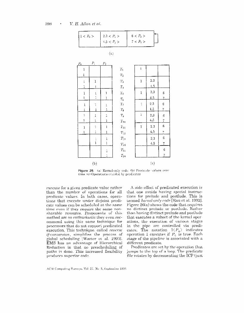
398 - V. H. Allan et al.
(a)
3
PIJ P* P2
1
1
1 1
1 1
1 i 1
1 1 1
1 1 1
1 1 1
1 1 1
1 1 1
1 1 1
1 1 1
1 11 1
1
1
T1
T2
T3
Ta
T5
T6
TT
T8
T9
TIO
T11
T12
T13
T14
T15
T16
1
1 2,3
4,5
1 2,3 6
4%5 7
1 2,3 6
4,5 ~
1 2,3 6
4,5 ~
1 2,3 6
4,5 7
2,3 6
4,5 7
6
7
(b) (c)
F%ure 26. (a ) Kernel-onlv code (b) Prcdlcate values over
Lime (c) Operations enabled by predicates
execute for a given predicate value ratherthan the number of operations for allpredicate values. In both cases, opera-tions that execute under disjoint predi-cate values can be scheduled at the sametime even if they require the same non-
sharable resource. Proponents of thismethod are so enthusiastic they even rec-ommend using this same technique forprocessors that do not support predicatedexecution. This technique, called reuerseif-con vers ton simplifies the process ofglobal scheduling [Warter et al. 1993].EMS has an advantage of HierarchicalReduction in that no prescheduling ofpaths is done. This increased flexibilityproduces superior code.
A side effect of predicated execution isthat one avoids having special instruc-tions for prelude and postlude. This istermed kernel-only code [Rau et al. 1992].Figure 26( a) shows the code that requiresno distinct prelude or postlude. Rather
than having distinct prelude and postludethat executes a subset of the kernel oper-ations, the execution of various stagesin the pipe are controlled via predi-cates. The notation 1( PO ) indicateso~eration 1 executes if P,, is true. Each. ,)
stage of the pipeline is associated with adifferent predicate.
Predicates are set bv the o~eration that.jumps to the top of a ‘loop. The predicatefile rotates by decrementing the ICP (just
ACL1 C!omputuw Surveys, TToI 27, N’CJ 3, September 1995

Software Pipelining “ 399
like the regular rotating register file).The predicate register file is shifted ev-ery 11 time steps. The code to set thepredicates always sets register specifierO, but because the physical registerchanges, all predicates are eventually af-fected. This logical predicate O (PO) is setto true in the prelude and is set to falsein the postlude.
If the code for our example is executedsix times, the predicates take on valuesindicated by Figure 26(b). PO is the logi-cal predicate pointed to by ICP ratherthan the physical register. Notice that inthe time step 3 the ICP has been decre-mented so the old value of PO becomesPI and the new logical PO is set. Thusboth are now true. Figure 26(c) shows theoperations that are executed at each pointin time.
2.4 Enhanced Modulo Scheduling
Although all modulo scheduling tech-niques are basically the same, they differin how they handle predicates. Hierar-chical Reduction schedules operations oneach branch of a conditional constructbefore combining using the union of therequirements. This prescheduling andunioning of requirements creates compli-cated pseudo-operations that are difficultto schedule efficiently with other opera-tions. Enhanced Modulo Scheduling usesif-conversion to convert all operationsinto straight line, predicated code. In thisform, scheduling is done noting that dis-joint operations do not conflict. There isno need to preschedule the various partsof the conditional construct. After moduloscheduling, modulo variable expansion isused to rename registers’ lifetimes fromdistinct iterations.
Predicated execution has the disadvan-tage that all operations from taken anduntaken branches are executed (even ifthe results are just thrown away). Thusthe resource requirement is the sum ofthe requirements of each branch. En-hanced Modulo Scheduling recreates thebranching structure, termed reverse if-conversion, by inserting conditionalbranch instructions to eliminate predi-
cated execution. In other words, predi-cated execution is used to allow opera-tions to be scheduled independently ofthe branching structure and then thebranching structure is reinserted. Thismethod has some real benefits in termsof simplicity, but is also hampered by thefact that such a techniaue is m-one to. .code explosion. If a predicated operation(predicated by p) happens to be sched-uled early, all imperative operations thatare between the first predicated opera-tion scheduled and the last operationpredicated on p must be cloned to ap-
Dear on each branch. If code that is m-ed-.~cated by p is overlapped n times, therecan be code expansion of order 2‘. Clearlythis is unacceptable. Various techniquesare employed to limit code explosion, themost important being the restriction ofwhich blocks are scheduled together. Theterm hvwerblock is used to denote whichset of” ‘blocks are scheduled together[Warter et al. 1992, 1993].
The initial simplicity of schedulingwithout regard to predicates results inthe complexity of introducing condition-als back into the code. Because the inser-tion of branches is done after codescheduling, various code inefficienciescan be introduced as is common when-ever phases are segmented. According toWarter et al. [1992], Enhanced ModuloScheduling performs 18% better than Hi-erarchical Reduction with UD to 105%.increase in code size. Although some ofthe increase in code size undo-ubtedly re-sults from the fact that tighter code over-laps more conditional constructs, some ofthe increase results from unnecessaryelongation of the predicated region.
3. KERNEL RECOGNITION
Although modulo scheduling algorithmscreate a kernel by scheduling one itera-tion such that it is legal when overlappedby H cycles, other techniques schedulevarious iterations and must recognizewhen a kernel has been formed. Someauthors term this type of softwarepipelining algorithm unrolling algo-rithms [Rau and Fisher 1993], but the
ACM Computmg Surveys, Vol 27, No 3, September 1995

400 “ V. H. Allan et al.
term kernel recognition is more accurateas there may be no physical unrollingpresent. Proponents of modulo schedul-ing point to the need to search for akernel as a flaw, whereas proponents ofkernel recognition counter that searching
for a pattern can be done with hashinglGand is much more efficient than repeat-ing the scheduling for various goal ini-tiation intervals. Kernel recognitionproponents also argue that the ability toachieve fractional rates effortlesslymakes their algorithms superior. Moduloscheduling algorithm enthusiasts claimthat the H rarely has to be incrementedover its original minimum initiation in-terval [Rau 1994]. Obviously, moduloscheduling can achieve fractional ratesby replicating the loop body beforescheduling. Howeverj this increases com-plexity and may result in full iterationsin prelude and postlude (that would beremoved).
A first attempt at kernel recognitiontechniques is to mimic what one mightattempt if one were scheduling by hand.The basic idea is to look at several itera-tions at a time and try to combine opera-tions that are not dependent on eachother. The steps are as follows:
(1)
(2)
(3)
Unroll the loop and note depen-dence.
Schedule the various operationsas early as data dependence al-low.
Look for a block of consecutiveinstructions that are identical tothe blocks after it. This blockrepresents the new loop body.Rewrite the unrolled iterations asa new loop containing the repeti-
tive block as the loop body.
The obvious question is “What do youdo if no block of repeating instructionssurfaces?” The URPR (UnRolling,Pipelining, and Rerolling) software
‘fi For the general resource model, hashing must bedone on an encoding of the entire state of the
scheduler at each point m time
pipelining algorithm, designed by Su etal. [1986] solves this problem using adhoc techniques to force a kernel by mov-ing duplicate operations before or after asection of code containing all operations.This moving of operations after schedul-ing introduces underutilized instructionsand produces inferior results. Su et al.[1987] developed an extension to the ba-sic URPR algorithm in which loops con-taining multiple basic blocks, abnormalentries, and conditional exits are han-dled. Unfortunately, the problems ofURPR are carried over into the morecomplicated version. Although it is inter-esting from an historical perspective,URPR is outperformed (in terms of tar-get code execution time) by other tech-niques. The next sections explain severalindependent kernel recognition type soft-ware pipelining algorithms.
3.1 Perfect Pipelining
Perfect Pipelining combines code motionwith scheduling. It achieves fractionalrates and handles general (dif, rein)pairs. Techniques to assist the formationof a pattern are somewhat ad hoc.
Historically, the effectiveness of localscheduling has been limited due to thesmall size of basic blocks. A new architec-tural model in which multiple tests canbe performed within a single instructiongreatly enhances the degree of paral-lelism achieved. Aiken and Nicolau[ 1988b, 1988c, 1990] introduce the Per-fect Pipelining algorithml~ for use withthis more general machine model [Aiken1988; Nicolau and Potasman 1990; 13re-ternitz 1991]. This method is importantin that it reframes the problem by chang-ing the parameters. It answers the ques-tion, “How would software pipelining be
17Aken does not consider Perfect P1pehnmg to bean algonthvz but rather a framework upon whichalgorithms can be built. Thus, for every reference to“the Perfect Plpehmng Algorithm,” the readershould substitute “one of many possible algorithmsusing the Perfect Plpehning framework “ The algo-rithm referenced is one that Aiken considers inAiken [ 1988]
ACM Computmg Surveys, Vol 27, No, .3, September 1995

Software Pipelining “ 401
IOl:z=x+y
02:y=5
03: w = a[i]
0~ ; if ccl
/\
Figure 27. Perfect Pipelining’s instruction model.
affected if the architectures were modi-fied to support it better?”
Perfect Pipelining is somewhat similarto the method of Su et al. in that the loopis prescheduled, unrolled, and over-lapped, but it is more sophisticated inthat operations may move independentlyafter the prescheduling and loops thatspan multiple blocks are easily accommo-dated. Perfect Pipelining (like EnhancedModulo Scheduling) is more powerfulthan previous techniques in that itcan take advantage of an architecturewith multiway branching. A multiwaybranching architecture allows an in-struction to have several branch targetlocations based on multiple Boolean con-ditions. Figure 27 illustrates a basic in-struction executable in one time unit inthis model. In one cycle, 01, Oz, and 03are executed and control is transferred toone of Iz, Is, or Id depending on thevalues of cc 1 and cc 2 (which are predi-cate set before this instruction). Suchinstructions are called tree instructions[Ebcio~lu and Nakatani 1990]. All theassignment operations are executed anda destination selected simultaneously. To
take advantage of this type of architec-
ture, a type of global code motion, called
migration, is implemented [Aiken andNicolau 1988a]. Migration is an improve-ment over early trace scheduling [Fisher1981] in that copies can be merged, andcode motion is tied to code correctingcompensation for that motion directly, sothe cost-benefit can be considered. Laterversions of trace scheduling have adoptedthese improvements [Freudenberger etal. 1994].
The types of code motion are enumer-ated in Fisher [1981]. The addition of theoperation to join multiple copies of anoperation as they move past a branchpoint, termed unification, is important inthat it reduces code explosion. The im-portance of unification is that the multi-ple copies of an operation generated bymoving past branch points can often berecombined.
Aiken and Nicolau perform global codemotion within the loop before softwarepipelining to simplify the initial sched-ule. Once global code motion has beenperformed, the loop is unrolled an un-specified number of times, and the resultis scheduled assuming infinite resources.In a loop, performing code motion beforeunrolling significantly speeds up pipelin-ing. The pipelining algorithm need notrepeatedly perform similar code motionswithin each copy.
The assumption of infinite resources inthe initial scheduling step is made be-cause the algorithm requires unham-pered motion. If the constraint of finiteresources is enforced and II, Iz, and Isare sequentially ordered, motion of anoperation between instructions Is and IIwould be limited by the fact that theoperation may not be able to temporarilyreside in instruction Iz because of re-source conflicts with the operations thatare placed there first. Thus instead ofallowing free code motion, the algorithmwould suffer from the race of which oper-ation got to node Iz first. The resultswould be somewhat history sensitive de-pending on the order operations movedrather than the best possible schedule.
ACM Computmg Surveys, Vol 27, No 3, September 1995

402 ● V. H. Allan et al.
ITERATIONS
(2,1)
(!)(0,3)
B—
(0,1)
1c
0,1)(1!1)
D3,1)
(1,1)
(a)
15
16
IT
18
IS
Ilo
111
1—
A
cDB
—.
2
A
BC
D
34
$
.4
A
B
cDB
D
(b)
5 6
T1A A
B
cDB
Figure 28. Similar nodes with different numbers of mtervenmg operations
Perfect Pipelining allows the patternto form natu~ally. & each succes~ive in-struction is scheduled, one must deter-mine whether the schedule has begun torepeat itself. Let the state of the scheduleat a specific instruction represent the setof information that controls which opera-tions may be scheduled in succeeding in-structions. For a general resource model,state must include resources committedby the previous scheduling of operationswith persistent resource requirements.For operations with nonunit latencies,state must include the concept of elapsedtime between dependent operations. Onemust determine if the new instructionthat has been generated is really neces-sary, or if a previous state in the sched-ule is the same as the current state. Iftwo nodes can be reduced to the samestate, they are said to be functionallyequivalent. An instruction that is func-tionally equivalent to an earlier node canbe replaced with a branch to the firstinstruction, thus creating a loop. Whenare two nodes functionally equivalent?Clearly the two nodes must look alike,but as Figure 28 demonstrates, that isnot sufficient. Although 12 and 16 areidentical, the state is different as suc-
ceeding instructions are not the same. Ifwe assume Iz, Is, IJ, and Is form a loop,operation B appears in this proposed loopthree times and all other operations ap-pear twice. Obviously, these instructionscannot form a loop as the postlude wouldnot be static but would have to be differ-ent depending on the number of itera-tions actually executed. The instructions16 and IT do form a loop, which is evidentfrom the fact that they keep repeatingduring the rest of the schedule.
Figure 29(b) illustrates a case in whichthe code between equivalent nodes repre-sents multiple iterations of the originalloop instead of exactly one iteration asseen in other algorithms. Although codespace is increased, the advantage is thatthe code can be scheduled more tightly.For example, in Figure 29(b) the advan-tage of having three copies of the loop in% is that instead of performing one itera-tion in two instructions, one can achievethree iterations in five instructions. Inthis case, the multiple iterations repre-sent an improvement. The ideal rate is ~,but if we require a single iteration in theloop, the execution time is [:1== 2. Wecannot achieve the ideal effective execu-tion time with modulo scheduling unless
ACM Computmg Surveys, Vol 27. No 3, September 1995

(a)
1,6,7
L(1.1)
6
(1,1)
7
(0,1)
8
2,4,5,8
m
3
(c)
Software Pipelining “ 403
1,4,6,7
2,5,8 7
3 1,6,8
2,4,5 1,7
3 2,5,6,8
3,4 1,6,7
2,4,5,8 7
3 1,6,8
2,4,5
3
(b)
11,61,71
31,22,5232,42
(d)
Figure 29. (a) DDG. (b) Result of Perfect Pipelining. (c) Results of modulo scheduling. (d) Resultof replicating three times before modulo scheduling
we replicate first (see Figure 29(d)). Inthis figure, each operation has been ex-panded into three operations (indicatedby a superscript) due to the replication.
In other cases, multiple iterations arepresent in the new loop body, but nobenefit is achieved. Figure 30 (a modifiedversion of Figure 9) shows a case inwhich this happens. The optimal result,in terms of execution time, that is foundwith modulo scheduling, is shown forcomparison.
Functionally Equivalent Nodes. LetX={x/, . . ..x~. x$} bethee the setofop-erations XJ from iteration i, that arescheduled at a given instruction [Aikenand Nicolau 1990]. In Figure 28(b), 11 isreferred to as the set {Bl, 132, Cz, A4} andthe next instruction is then set {llz, B 3}.Two instructions are similar if they con-
tain the same operations and the super-scripts for the same operation differ by atmost a constant. If X = {.. . ,x~J, . . .}, letX’={..., xy,’,. ..}. Although similarityis necessary for functional equivalence, itis not sufficient. Functionally equivalentnodes are two nodes that can be usedinterchangeably in the schedule graph.Two instructions that are similar are notalways functionally equivalent. We canfind two similar instructions X and Y byhashing, 18 but one has to compare thestate (including resources committed bypersistent irregular operations) at X and
lS Hashing is a search technique m which a func-
tion of the key is used to determine the storagelocation. Two instructions that have the same con-
tents hash to the same location, and hence areeasily identified.
ACM Computmg Surveys. Vol 27. No 3, September 1995

404 . V. H. Allan et al.
(0,1)
1,3,4
2,5 4
16 1,3,5
7 2
6
7
(b)
(a)
1,3,4
2.5
IIzzl6’7
(c)
Figure 30. (a) DDG, (b) Result of Perfect Pipelining. (c) Result of modulo schedulingalgorlthm.
Y to ensure functional equivalence. Earlyversions of this algorithm were limitedby the fact that true functional equiva-lence was not guaranteed.
For example in Figure 28, althoughIz = {Cl, A3} and lG = {C3, A5} are simi-lar, the next instructions scheduled aredifferent; no repeating pattern hasformed. In the DDG of Figure 31, we seea case where the lack of similarity indi-cates the nodes are not functionallyequivalent. The cycle involving nodes 1and 2 is initiated every instruction, butthe cycle involving 3, 4, and 5 repeatsevery three instructions. Although nodescontaining the same operations are found
(11 and I,), they are not similar in thateach pair of operations in the two in-structions do not differ by a constantsubscript. Thus the procedure to find twofunctionally equivalent nodes must in-clude full state information.
If we have two dependence cycles capa-ble of different execution rates, as seen
in Figure 31, we must slow the faster onedown in order to get a pattern. This isaccomplished by forcing the set of opera-tions considered for scheduling to containonly operations from a fixed range ofiterations. Let Span be the limit that in-dicates that until all operations from it-eration i have been scheduled, opera-tions from iteration i + Span cannot bescheduled. Stated another way, if opera-tion a has been scheduled s. times andoperation b has been scheduled s~ times,then ls~ – Sal < Span The value of Spanis experimentally determined. If Span istoo small, a schedule does not form. IfSpan is too large, the prelude andpostlude are overly complicated. Theschedule of Figure 3 l(b) results whenSpan = 4. Notice that 17 is delayed until33, 43, and 53 have been scheduled.
When Perfect Pipelining is applied to aloop body consisting of a single basic blockwith unlimited resources, a time optimalpipeline is formed. The other methods
ACM Computmg Surveys, Vol 27, No 3, September 1995

Software Pipelining “ 405
C7!?(1,1) 1
(!)(0,1)
2 a3 11: 1,3
(0,1) 12: 2,4 1
IJ 5 2
4 14: 3
(0,1) 15: 4(1,1)
16:~
5 17:
I*:
19:
110:
(a)
1
2 1
2 1
L_._J-l3 1
(b)
Figure 31. An acceptable pattern may not occur without intervention. (a) DDG. (b) Pipelining with
Span = 4.
may not always form a time optimalpipeline because they force % to containa single copy of each operation that maydelay the start of the next iteration. Onthe other hand, when using the greedyscheduling algorithm, Perfect Pipeliningwaits for a pattern to naturally develop.Therefore, when L consists of a singlebasic block and resources are unlimited,it always produces a time optimalpipeline.
An Example. To see the power ofthis technique, one must considerbranches within the loop. Consider thepiece of code shown in Figure 32 (takenfrom Aiken [1988]) that builds a list.Each call to append is dependent on theprevious call to append, and hence isserialized.
If the first seven iterations of the loopare scheduled, assuming three tests canbe performed in one instruction, the exe-cution graph of Figure 33 results in whichnodes represent parallel instructions andarcs represent the flow of control. Thesuperscript on each operation representsthe iteration number of the operation.Notice there are several branches leavingeach instruction. The arc labels corre-spond to the values of the tests. The label“fft” indicates the first two tests are falseand the last test is true. An asterisk
Fori=l ton
T: If B[i] = key
A: list = append(list,i)
Figure 32. Sample code.
indicates a “don’t care” condition. To re-duce the number of different instructionformats, whenever an append is per-formed, the tests for the three successiveiterations are executed, even if some havealready been performed. Notice that theability to perform multiple tests in a sin-gle instruction greatly reduces the execu-tion time of the loop in cases where theappend operation does not occur for ev-ery value of i. After equivalent nodeshave been identified, the graph of Figure34 shows the final result of PerfectPipelined scheduling.
3.2 Petri Net Model
The Petri net algorithm uses the richgraph-theoretic foundation of Petri netsto solve the problem of kernel recogni-tion. It achieves fractional rates, worksfor general (dif, min ) pairs, and isextendible. It has the power of Per-fect Pipelining, but has replaced ad hoctechniques with mathematically soundapproaches.
ACM Computmg Surveys, VO1 27, No 3, September 1995

406 e V. H. Allan et al.
t**
ff
i‘
fft
Figure 33. Loop after unrolhng seven times
fffi=i+3
ffft fft
i=i+4 f~ * i=i+2i=i+l
fft
[
i=i+3~, 1+1 l-+ r@3
b 4
t** ft *i=i+l i=i+2
Figure 34. The same loop (Fig. 33) after plpelmmg
ACM Computing Survey,, Vol 27, No 3, September 19c15
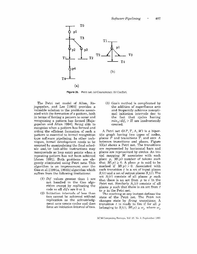
Software Pipelining “ 407
ITO
T2T2
1’p4
%’1
&
pl
T4
(b)
T&
(a)
Figure 35. Petri net. (a) Concurrency. (b) Conflict.
The Petri net model of Allan, Ra-jagopalan, and Lee [1993] provides avaluable solution to the problems associ-ated with the formation of a pattern, bothin terms of forcing a pattern to occur andrecognizing a pattern has formed [Raj a-gopalan and Allan 1994]. Being able torecognize when a pattern has formed andaiding the efficient formation of such apattern is essential to kernel recognitiontype software pipelining. In other tech-niques, kernel development needs to beassisted by manipulating the final sched-ule and/or look-alike instructions maymasquerade as loop entry points when arepeating pattern has not been achieved[Jones 1991]. Both problems are ele-gantly eliminated using Petri nets. Thisalgorithm is an improvement over theGau et al. [1991a, 1991b] algorithm whichsuffers from the following limitations:
(1)
(2)
Dif values greater than 1 arenot handled in the Gao algo-rithm except by replicating thecode so all difs are O or 1.
Initiation intervals of less thantwo cannot be achieved withoutreplication as the acknowledg-ment arcs create cycles and thusforce an initiation interval of two.
T3
(3) Gao’s method is complicated bythe addition of superfluous arcsand frequently achieves nonopti-mal initiation intervals due tothe fact that cycles havingminQ/dife > II are inadvertentlycreated.
A Petri net G(P, T, A, M) is a bipar-tite graph having two types of nodes,places P and transitions T, and arcs Abetween transitions and places. Figure35(a) shows a Petri net. The transitionsare represented by horizontal bars andplaces are represented by circles. An ini-tial mapping M associates with eachplace p, M(p) number of tokens such
that M(p) >0. A place p is said to bemarked if M(p) > 0. Associated with
each transition t is a set of input placesS,(t) and a set of output places SO(t). Theset S,(t) consists of all places p suchthat there is an arc from p to t in thePetri net. Similarly SO(t) consists of allplaces p such that there is an arc from tto p in the Petri net.
The marking at any instant defines thestate of the Petri net. The Petri netchanges state by firing transitions. Atransition t is ready to fire if for all pbelonging to S,(t), M(p) > WP where WP
ACM Computing Surveys, Vol 27, No 3, September 1995

408 0 V. H. Allan et al.
is the weight of the arc between p and t.The reader may see some similarity be-tween transitions and runners in a relayrace. One runner cannot run (fire) untilhe has been given the baton (token).However, in this case, a runner can passa baton to several teammates simultane-ously and one runner may have to re-ceive a baton from each of several team-mates before running.
When a transition fires, the number oftokens in each input place is decre-mented by the weight of the input arcwhile the number of tokens in each out-put place is incremented by the weight ofthe arc from the transition to that place.All transitions fire according to the earli-est firing rule; that is, they fire as soonas all their input places have sufficienttokens. In Figure 35(a), there are no arcsbetween transitions TI and T2. Thesetransitions are independent of each otherand can be fired concurrently. However,Ti cannot fire until TI has fired andplaced a token in place pl. Therefore, TAis dependent on T1. In Figure 35(b), place
P 1 contains only one token which can beused to fire one of transitions T2, T:j, orTJ. This represents a conflict that can beresolved using a suitable algorithm.
The Petri net models the cyclic depen-dence of a loop. A data dependence graphshows the must-follow relationship be-tween operations (nodes). However, itcannot show which operations are readyto be scheduled at a given point in time.A Petri net is like a DDG with the cur-rent scheduling status embedded. Eachoperation is represented by a transition.Places show the current scheduling sta-tus. Each pair of arcs between two tran-sitions represents a dependence betweenthe two transitions. When the place (be-tween the transitions) contains a token,it is a signal that the first operation hasexecuted, but the second has not.
The firing of a transition can bethought of as passing the result of anoperation performed at a node to othernodes that are waiting for this result. Ifthe Petri net is cyclic, a state may bereached when a series of firings of thePetri net take it to a state through which
it has already passed. The state of thePetri net is represented by the tokencount at each place. Because all decisionsare deterministic, an identical state (withan identical reservation table) means thebehavior of the Petri net repeats.
Min values of greater than 1 are han-dled by inserting dummy nodes so thatno min is greater than 1. For example,an arc (a ~ b, dif, 3) is replaced by arcs
(a - tl, dif, 1), (tl - tz, O, 1), and (t2+b, O, l), where tl and t2 are dummynodes. This implementation increasesthe node count, but greatly simplifies therecognition of equivalent states as themarking contains all delay information.This algorithm handles min values ofzero by doing a special firing check fornodes connected to predecessors by mintimes of zero. Thus compile time is in-creased by accommodating min times ofzero.
Arcs are added to the DDG to makethe graph strongly connected, eliminat-ing the problem of leading chain synchro-nization. The benefit is that the rate ofeach firing is controlled; no node is al-lowed to sustain a rate faster than theslowest cycle dictates. As arcs are added,new cycles are created. If a new cycle 9‘has a larger min ~ /dif~ than that con-tained in the original graph, the scheduleis necessarily slowed down (II increased).
For simplicity, the number of addedarcs is kept to a minimum. Formally, thisis done as follows. If D is the DDG, letD‘ represent the acyclic condensation ofD in which each strongly connected com-ponent of D is replaced by a single node.For a node d‘ ● D‘, there exists a set ofnodes Cd c D that correspond to d‘. Ifthere is a single source nodelg in D‘, let
s‘ be that node. Let s be arbitrarily se-lected from C,. If there is more than onesource node in D‘, create a set of nodes
R c D in which each source node of D‘has a corresponding node. Let s be adummy node added to D. For each r E R,add an arc (s ~ r, 1, 1) to the DDG. For
lY A source node has no predecessors
ACM Computmg Surveys, Vol 27, No 3, September 1995

Software Pipelining . 409
(1,1
d6
(1
(a)
(b)
pl
g~-
p8. p7.“ pl
T6 T1plo
.p5 po
—2 T2
IT!lip2
T3
p4 . P3
T4
T5
t--J5.l(c)
Marked Places (tokens) Schedule
o 4(1),5 (1),7(1),8(1),9(2),10(1) 1, 6
1 O(l), l(l), 4(l), 5(1),6(1), 9(2),10(1) 2, 5
2 2(1),4(1),5(1),7(1), 8(1),9(1),10(1) 6
3 0(1),1 (1),3 (1),5 (1)>6(1),9(1),10 (1) 4 2; 5
4 2(l), 4(l), 5(l), 7(l), 8(1),9(1),10(1)
(d)
Figure 36. (a) DDG. (b) After being made strongly con-nected. (c) Petri net. (d) Schedule assuming infinite re-sources
each node k‘ = D‘ which is a sink,20 ar- selected so that any cycle (3 formed has abitrarily select node k = C~ ~ and add an mine/dif8 ratio as close as possible to thearc (k - s, dif, 1). The values of dif are lower bound for II without exceeding it.
For example, in Figure 36(b) the DDG ofFigure 36(a) is made strongly connected.
‘0A sink has no successors. The acyclic condensation consists of nodes
ACM Computing Surveys, Vol. 27, No. 3, September 1995

410 “ V. H. Allan et al.
(representing the sets of nodes from theoriginal graph) {l}, {2}, {3, 4}, {5}, and {6}.The nodes of the acyclic condensation {1}and {6} are both sources. Thus a dummynode 7 is created as s and arcs (7 - 6, 1,1) and (7 ~ 1, 1, 1) are added. The nodesof the acyclic condensation {6}, {3, 4}, and{5} are sinks. One node from each of theacyclic condensation sink nodes is con-nected to node 7. This results in addingarcs (6 ~ 7, 0, 1), (4 ~ 7, 2, 1), and (5 ~7, 1, 1) to the DDG. Dif values are se-lected to force newly formed cycles tohave minti/diffl <2.
Once the DDG has been modified sothat it is strongly connected, the corre-sponding Petri net is created. Basically,nodes become transitions in the Petri net,each arc becomes a pair of arcs in thePetri net, and places are inserted be-tween dependent transitions to keeptrack of what may fire next. The formalrules are as follows:
(1)
(2)
For each node i in the DDG, atransition T, is created.
For each arc in the DDG fromnode i to node 1“, a place p iscreated along with arcs from T,to p and from p to T].
At each point in time, the transitionsthat fire form a parallel instruction ofthe schedule. When the marking repeats,a software pipeline exists. The schedulerepeats whenever the Petri net enters astate (defined by the placement of to-kens) in which it has been before. For agood discussion of the properties of cyclicPetri nets, see Gao et al. [ 1991b].
The initial placement of tokens mustbe specified. Initially, any node that isdependent on a previous iteration isready to be executed (as there is no pre-vious iteration to deny execution). Thusone would guess that places that modelarcs representing loop-carried depen-dence would need to be marked. Thequestion comes in deciding how manytokens should be placed there. The num-ber of tokens necessary depends on thedif value for that arc. A dif of zero corre-sponds to ~zo tokens. Let b‘ represent
operation b from the i ‘h iteration. A difof three on arc a ~ b indicates that bcan get three iterations ahead of a. Thusb’ must follow al; yet, bl, bz, and bJ areunconstrained. Therefore, the number oftokens at a place is just the dif of thecorresponding arc in the dependencegraph. The formal rule follows.
(3) The initial marking of the Petrinet is such that for an arc from z
to j in the DDG with dif valued, the corresponding place p hasd tokens assigned to it. This al-lows node T] to be fired up to dtimes before node T, is fired.
Modeling Resources. Any restric-tion (other than dependence) is modeledas a resource constraint. If we had asingle adder, operations needing theadder could not be scheduled together.Resource usage that is regular or nonper-sistent can be handled by introducingresource places. The rules governing re-source places are as follows:
(4)
(5)
For each resource, a place p, iscreated. The place is assigned thesame number of tokens as thenumber of instances of that par-ticular resource.
Resource usage is controlled byrequiring that all nodes needingthe resource be cyclically con-nected to this place. If a nodeuses a particular resource, thenthere is a loop from that transi-tion to the resource place andback. Because a node needs a to-ken on each of its input placesbefore it can fire, an arc froma resource place requires thatthe resource is available beforescheduling the node. The arc tothe resource place allows thenode to return the resource afteruse. 21
‘1 If an operation required more than one instance
of a gwen resource, the arcs could be weighted withthe number of tokens reqtured from that source
ACM Computmg Surveys, Vol 27. NrJ 3 September 1995

Software Pipelining “ 411
Modeling persistent irregular resources
requires a more complicated model. In-
stead of using resource places (that canonly ensure a resource is available at agiven point in time, not future availabil-ity) a current reservation state must bekept. A reservation state (RS) is the unionof all reservation tables (offset to reflectstarting time) for operations that havebegan execution but have not completed.Consider an operation a that is to bescheduled. If the corresponding reserva-tion table R ~ has length If?. 1, each rowmust be intersected (binary and) withthe corresponding row of the reservationstate. If any resulting row is nonzero,there is a resource conflict and the opera-tion cannot be scheduled. If there are noconflicts, each row is unioned (binary or)with the corresponding row of the reser-vation state to reflect the current andfuture resource needs. After all opera-tions for the current time cycle have beenscheduled, the reservation state is ad-vanced to reflect the passage of time,that is, RS[i] = RS[i + 1] Vi = O... IRSI– 1.
Behavior Table. The scheduleshown in Figure 36(d) is termed the be-havior table. Row O of Figure 36(d) indi-cates the initial marking of each place inthe Petri net; the number of tokens ateach place is shown in parentheses. Thecolumn marked “Schedule” indicates thetransitions that fire given the currentmarking. For simplicity of presentation,it is assumed there are no resource con-flicts. As the state at instruction 2 andthe state at instruction 4 are identical,the kernel starts at instruction 2 andends at instruction 3, The kernel with aninitiation interval of two is marked witha box. In order to incorporate persistentirregular resource usage, each row of thebehavior table has an attached resourcestate describing the current and futureresource commitments. For simplicity,the attached resource state (dummytransition 7) is not shown.
This algorithm is enhanced by the ad-dition of a pacemaker that regulates thegreediness of the algorithm [Allan et al.
1993]. A pacemaker is a cycle of dummy
nodes added to the Petri net that has amin@/difti equal to the estimated H. Thepacemaker passes tokens to the rest ofthe Petri net to control the rate of firing.The pacemaker attempts to force the es-timated pace so a repeating section isformed quickly. In the example of Figure36(b), a pacemaker to ensure that nodesdo not fire more frequently than everytwo cycles is not required as the scheduleexhibits that property already. In largerexamples, a pacemaker can reduce thecompile time to obtain the schedule, theSpan for the kernel, and the achievedinitiation interval.
This general model for software pi-pe-lining has the advantage of being easilyextendible. For example, predicates
within the loop body are handled bypassing the token along paths represent-ing both the branches and by having amerge node that does not fire until itreceives a token from both branches. Thecontrol dependence itself is treated as aform of data dependence. The Petri NetPacemaker (PNP) technique performsoptimizations such as renaming and for-ward substitution to improve the perfor-mance of loops containing predicates
[Rajagopalan and Allan 1994].The Petri net approach solves the prob-
lem that &ken and Nicolau [ 1988c] andZaky [1989] faced of having two parts ofthe graph execute at different rates.Making the graph strongly connectedforces all transitions to fire at the samerate. The number of tokens at eachresource place reflects the number ofresources of each type. Thus when atransition fires, all other transitionscompeting for the same resource areprohibited from firing as the token isnot available. To maintain determinism,the selection algorithm must beconsistent in choosing which candidatesfire when there are competing choices.The priorities used in scheduling aresimilar to other scheduling algorithms.Each transition is augmented with anexecution count that is incremented eachtime the transition fires. When severaltransitions are able to fire, the selection
ACM Computmg Surveys, Vol. 27, No 3, September 1995

412 “ V. H. Allanet al.
algorithm is able to fire the transitionthat has fired least and hence is from theearliest iteration. Transitions are alsoprioritized so that within the same itera-tion, transitions that are part of criticalcycles are selected first.
The Petri net approach also solves theproblem of persistent irregular resources.The procedure to identify an identicalstate is broken down into steps. Step oneuses hashing on the encoding of the to-kens at each place to discover when thetokens are in an identical configuration.For each state on the matching hash list,step two checks to see if the current globalreservation table agrees with the globalreservation table at the previous step.For a sufficiently large hash table, thenumber of entries to check is small (oneor two) and the test for an identical stateonly proceeds until a single elementdiffers, so the check for identical staterequires minimal effort.
Comparison With Other Methods.PNP is similar in spirit to PerfectPipelining [Aiken and Nicolau 1988a,1988b; Nicolau and Potasman 1990]. Aproblem for Perfect Pipelining is the dif-ficulty of determining when nodes arefunctionally equivalent (i.e., the patternis repeating). Because the Petri net usesa combination of places and global reser-vation tables to record state information,a repeating pattern can reliably be deter-mined. Perfect Pipelining also createskernels in which duplicate operations arepresent even when doing so does not im-prove performance. For example, a looplength of 4 with two copies of each opera-tion (for an effective initiation interval of2) is generated when a loop length of 2
(with one copy of each operation) isequivalent. This results from the prob-lem of scheduling each node greedily. Be-cause each node is allowed to execute asfast as possible as long as gaps do notoccur in the schedule (preventing a pat-tern from forming), some operations arescheduled more frequently than the ef-fective initiation interval. Later, otheroperations have to be delayed to satisfydependence constraints. Inasmuch as the
pacemaker regulates the rate of all oper-ations, such rate fluctuations (that in-crease the code size) are less likely. For athorough discussion of these problems seeJones and Allan [ 1990].
The PNP algorithm is compared withLam’s algorithm on loops with both lowand high resource conflicts [Rajagopalanand Allan 1994]. With low resource con-flicts, the PNP algorithm does marginallybetter. With high resource conflicts, thePNP algorithm shows a significant im-provement of 9.27c over Lam’s algorithm.PNP often finds a lower H as fractionalrates are required. Because Lam’s algo-rithm schedules each strongly connectedcomponent separately, a fixed ordering ofthe nodes belonging to each strongly con-nected component in the schedule is used.This fixed ordering, together with theresource conflicts between the nodes ofthe strongly connected component andother nodes of the schedule, restricts theoverlap between them. This forces Lamto use a higher value of H which inmany cases is not optimal.
The PNP algorithm is compared withVegdahl’s [ 1992] technique that performsan exhaustive search of all the possibleschedules to look for a schedule with theshortest length. PNP compares quite fa-vorably with this exhaustive technique.The compile time of PNP is negligi-ble compared to Vegdahl’s exhaustivetechnique.
3.3 Vegdahl’s Technique
Unlike all other techniques discussed inthis survey, Vegdahl’s represents an ex-haustive method in which all possiblesolutions are represented and the best isselected. As software pipelining is NP-complete, this makes the algorithmimpractical for real code.
Vegdahl [ 1992, 1982] uses an exhaus-tive technique that relies on a decisiongraph of choices. The method uses a dy-namic programming scheduling algo-rithm to schedule straight line codeformed from the loop body by unrolling.Vegdahl builds an operation set graph inwhich nodes represent the set of opera-
ACM Computing Sur>eys, Vol 27, No ‘3, September 1995

Software Pipelining “ 413
Figure 37. Partial operation set graph for the example of Figure 28.
tions scheduled so far and arcs representa series of scheduling decisions. Inessence, the nodes represent state infor-mation similar in usage to the markingsin the Petri net algorithm, the differencebeing that the operation set graph repre-sents all possible scheduling decisions atevery point in time rather than a singledecision. Although the concept is like adecision tree [Smith 1987], the diagrambecomes a graph because nodes repre-senting equivalent states are merged.Rather than considering loop-carried an-tidependences directly, Vegdahl defines“duals” of the dependence to representantidependences. This appears to be anidiosyncrasy of the data representationrather than an inherent part of the con-cept. The automatic interpretation of de-pendence arcs is a disadvantage if reg-ister renaming eliminates loop-carriedantidependences.
Consider the partial operation setgraph for the example of Figure 37, Be-cause the graph is so large, only repre-sentative parts of it are shown. Inasmuchas the span of the schedule obtained byPNP is two, it is reasonable to applyVegdahl’s exhaustive technique to a loopbody that has been unrolled twice (twocopies exist) as this allows operationsfrom adjacent iterations to be scheduled
together. Initially no operations havebeen scheduled (represented by the ini-tial node with no label). There are threechoices: 1 can be scheduled, 6 can bescheduled, or both 1 and 6 can be sched-
uled. These three choices are representedby three arcs emanating from the initialnode. Suppose 6 is scheduled first, thenthere are three choices for the next timestep: 1 can be scheduled, operation 6 fromthe next iteration (6’) can be scheduled,both 1 and 6’ can be scheduled. Thesechoices are represented by arcs comingout of the node labeled 6. Note that thenode labeled 6 indicates operation 6 hasbeen scheduled, and an arc labeled 6 in-
dicates 6 is to be scheduled at this timestep. If 6 is scheduled in the first timestep and then 1 is scheduled in the sec-ond time step, the node 16 is reached.Notice this is the same node reachedif operations 1 and 6 were scheduledinitially. The scheduling process is asfollows:
(1) Create an empty initial node andmark it as open.
(2) While there exists an open node,select an open node curr.
(a) While observing both re-source conflicts and depen-
ACM Computing Surveys, Vol. 27, No. 3, September 1995

414 “ V. H. Allanet al.
(3)
dence constraints, considerall possible operations thatcan be scheduled given theoperations of curr have exe-cuted. Let exec be one possi-ble set of operations that canbe executed. Let next repre-sent the new state formedfrom executing exec whencurr was the previous state.If next contains every op-eration from one iteration,reduction is applied by re-moving the set of operationsand shifting the remainingoperations by one iteration,for example, x‘ becomes x,
x“ becomes x‘. (In our exam-ple, when we execute 42’5’ atnode 123561’6’ this results innode 1256 rather than1234561’2’5’6’.) If next is al-ready in existence as a node,create an arc from curr to
that node with label exec.Otherwise, create a new noderepresenting next and createan arc from curr to next withlabel exec and mark the newnode as open.
(b) Repeat the preceding step foreach possible set exec.
Once there are no more o~ennodes, locate all cycles in ‘thegraph. Cycles of minimum lengthare possibilities for the kernel ofthe software pipeline.
Kernel recognition is handled by themerging of equivalent nodes followed byfinding minimal cycles. In our example,one cycle (shown in bold) consists of in-structions 31‘ 6‘ and 42’5’ and representsthe same kernel found in Figure 36(d).Another possible schedule is shown bythe schedule 31‘ and 42’5 ‘6’. A nonopti-mal schedule is indicated by 2, 361’, and45’. Numerous other possibilities existbut have been omitted from the opera-tion set graph in the interest of readabil-ity. This method does not generateprelude or postlude, although this codecan easily be generated given the kernel.
In order to evaluate which cycle of mini-mal length is best, prelude and postludecode must be considered.
Because the algorithm is exhaustive, itproduces optimal results but is obviouslyinappropriate for graphs of any size. Thealgorithm works best when the graph istightly constrained and has many re-
source conflicts as fewer state nodes inthe operation set graph are possible. Thisalgorithm has many similarities to thePetri net algorithm. Min values ofgreater than one are implemented by in-troducing dummy nodes. Vegdahl [1992]states that dif values of greater thanone can be handled, but this has not beenfully tested. Although the use of dummynodes addresses the problem of nonunitlatencies, persistent resource usage can-not be modeled. Although Vegdahl nevermentions fractional rates, this methodclearly has the potential of achievingfractional initiation intervals. Vegdahl’salgorithm differs from the Petri net algo-rithm in its exponential time complexityas well as in the fact that it physicallyunrolls the loop a “sufficient” number oftimes before the algorithm begins. Anupper bound on the number of nodes inthe operation set graph is the cardinalityof the power setzz of the set containingall operations of the unrolled loop. Be-cause the size of the unrolled loop mayhave such a negative effect on the com-plexity, it is important to be able to pre-dict the amount of unrolling necessary toachieve an optimal schedule. Many ofthese nodes are never present in the op-eration set graph as they do not repre-sent a legal state in the firing sequenceconstrained by dependence and resourceconflicts.
Predicates have not been implementedbut the author alludes to the possibilitythat conditionals could be handled bycombining the algorithm with tracescheduling.
‘4A power set of set P IS the set of all subsets of 2?For a set F’ having p elements, the power set has2/’ members.
ACM Computing Survey., Vol 27, No 3, September 1995

Although this algorithm is impractical
because of its complexity, it may be use-ful for very small examples, and it under-scores the reason that researchers lookfor heuristics.
4. ENHANCED PIPELINE SCHEDULING
Enhanced Pipeline Scheduling integratescode transformation with scheduling toproduce excelle~t results. One importantbenefit is the ability to schedule variousbranches of a loop with different II.
Ebcio~lu and Nakatani [1990, 1987]propose an algorithm unlike either mod-U1Oscheduling or kernel recognition algo-rithms. Enhanced Pipeline Schedulinguses a completely different approach tosoftware pipelining, building on codemotion (like Perfect Pipelining), but re-taining the loop structure so no kernelrecognition is required. This algorithm isquite complicated both to understand andin the code produced. However, it hasbenefits no other algorithm achieves as itcombines code transformation with soft-ware pipelining.
Code motion pipelining can be de-scribed as the process of shifting opera-tions forward in the execution schedule.Because operations are shifted throughthe loop control predicate, they moveahead of the loop, into the loop preludeand they move back into the bottom ofthe loop, as operations from a later itera-tion. The degree to which shifting is ableto compact the loop depends on the re-sources available and the data depen-dence structure of the original loop. Thealgorithm has some similarity to PerfectPipelining in that it uses a modificationof Perfect Pipelining’s global code motionalgorithm, but differs significantly be-cause Enhanced Pipeline Schedulingmanipulates the original flow graph tocreate z and does not require searchingfor a pattern in unrolled code. Becausethe loop is manipulated as a whole ratherthan as individual iterations, Enhanced
Pipeline Scheduling does not encounterthe problems of pattern identification in-herent in Perfect Pipelining.
Software pipelining occurs when oper-
Software Pipelining “ 415
ations are moved across the back edge,23allowing them to enter the loop body asoperations from future iterations. Thepipelining algorithm iterates until all theloop-carried dependence have been con-sidered, The pipeline prelude and post-lude are generated by the automatic codeduplication that accompanies the globalcode motion.
This model can handle min times ofgreater than 1 by inserting dummy nodes.However, the algorithm cannot handlepersistent irregular resources.
4.1 Instruction Model
Enhanced Pipeline Scheduling is apowerful algorithm that can utilize amultiway branching architecture withconditional execution. The conditional ex-ecution feature makes this machinemodel more powerful than the originalPerfect Pipelining machine model thatincludes only multiway branching. Re-cent versions of Perfect Pipelining haveincluded multipredicated execution[Nicolau and Potasman 1990]. In order totake advantage of multipredicated execu-tion, a more powerful software pipeliningalgorithm is required.
Figure 38 shows a typical control flowgraph node,24 11, termed a tree instruc-tion. 12 through 14 are labels of othercontrol flow graph nodes. The conditioncodes ccl and CC2 are computed beforethe node is entered, and only those state-ments along one path from the root to aleaf are executed. All the operations onthe selected path are executed concur-rently, using the old values for alloperands. For example, in Figure 38 ifccl is true (left branch) and CC2 is falsewhen II is executed, operations 01, 03,OT, and OS are executed simultaneously,
23A back edge of a data dependence graph is an
edge whose head dominates its tail in the flowgraph and is used to locate a natural loop [Aho etal. 1988]. A node a dommates a node b m a graph If
every path from the source to b must contain a24A Control Flow Graph (CFG) M a graph in whichnodes represent computations and edges representthe flow of control [Aho et al. 1988].
ACM Computmg Surveys, Vol 27, No 3, September 1995

416 “ V. H. Allan et al.
05: if CC2 1 12 1L ---- 1
/\
o~:t=t–1of3:y=o
Os : a[z] = t
~----,1131L ---- J
r ---- 1I 14 IL---- J
Figure 38. Tree mstructlon used m enhanced Dmelme
scheduhng.
then control is transferred to 11. Thusthe assignment to t by OT does not effectthe use of t by Og. Two types of resourceconstraints are placed on this machinemodel. One is limited by the total num-ber of operations that can be containedwithin the tree instruction. One is alsolimited to a fixed number of differentpaths through the tree instruction.
With conditional execution, operationscan be placed on any branch of a CFGnode, unlike a traditional machine modelin which all operations must precede anyconditional branch operations. AlthoughEnhanced Pipeline Scheduling can uti-
lize such features, the scheduling tech-nique does not require this powerful ar-chitecture. Other architectures can berepresented by the tree instruction byrestricting the form of the instruction.For example, architectures that do notsupport multi way branching or condi-
tional execution can be modeled lby treeinstructions.
4.2 Global Code Motion With Renami[ng andForward Substitution
Nakatani and Ebcioglu [ 1989] use re-naming and forward substitution25 to
—
25The authors term this combmmg,
. .
move operations past predicates and
shorten dependence chains involving an-
tidependences. Renaming involves re-
placing an operation such as x = y op z
with two operations x‘ = y op z; x = x‘.Because x‘ = y op z defines a variablethat is only used by the copy statement
x =x’, the assignment to x is free to
move outside the predicate. When x‘ =
y op z moves before the predicate that
controls its execution, the statement is
said to be speculative because the state-ment is only useful if the branch is taken.
Figure 39 illustrates the shortening of adata dependence chain (involving an an-tidependence) and a control dependence
chain using renaming of a. Figure 39(a)shows the original dependence graph,
whereas Figure 39(b) shows the graph
after renaming. The dependence betweenn3 and n4 can be eliminated by forward
substitution. For an assignment state-
ment var = expr, when uses of var insubsequent instructions are replaced byexpr, it is termed forward substitution.This is particularly useful if, as a resultof the forward substitution, the opera-
tions can be executed simultaneously. InFigure 39(c) forward substitution is used
to change d = 2*a to d = 2*a’ becausethe a referenced has the value of a‘.
ACM Computmg Surveys, Vol 27, No 3, September 1995

m
+a
ACM Computmg Surveys, Vol 27. No 3, September 1995

418 . V. H. Allan et al.
Oz : if ccl Oz : if ccl
f
2
0B:CC2=Z<Y
04: X=Z+4
4
&’>,--J
+
Os:cc2=Z<y04: X=Z+4
06:ya=z+6
4
+0,s : if CC2
7’\OG:y =x+0~ : z = a[y] Oc~:y=y.
/\
07: z = a[y]
08: y = a[x]Og:z=ya+w
08: y = a[z]
T5 if;i
L--J
09:z=y*w
----
:17j--
Figure 40. Example of code motion of 06x=z+4forthexln 06.
Figure 39(a) shows that d = 2 * a is re-
named. Notice that in this case the length
of the dependence chain for the graph isdecreased.
To see the flexibility of this model, node
2 could also represent a predicate andthe same transformations used on the
data dependence also can be applied tothe control dependence.
Forward substitution may collapse truedependence that prevent code motion. A
true dependence between two operations01 and Oz may be collapsible with for-ward substitution if (1) O ~ is a copy oper-
ation, or (2) both operations involve aconstant immediate operand. Forwardsubstitution is performed if a true depen-
dence can be collapsed.
Figure 40 shows an example in whichboth forward substitution and renamingare required to move an operation. The
with renaming and forward substitution of
diagram shows part of a CFG before and
after operation Oc is moved from instruc-
tion 14 to instruction Iz. Note that multi-ple tree instructions are shown in thefigure. Each rectangular node is the en-try point of a tree instruction. Dashedboxes represent branches to the treeinstructions indicated. OG has a true de-
pendence on 04 that involves an immedi-
ate operand, making this dependence acandidate for forward substitution. First,
y is renamed giving Oc : y. = z + 6 ando ~a : y = y.. Next, forward substitutionis performed giving OG : y = z + 4 + 2.Constant folding is then performed giv-ing OG : y = z + 6. To see the advantageof this renaming, Og is moved from 15eliminating 15. This motion requires for-
ward substitution as Oq : z = y. * w. No-tice that the total execution time of the
code has been reduced.
ACM Computing Surveys, Vol 27 No 3, September 1995

Software Pipelining “ 419
JA a= b[i]+c
(0,1)
B d(i] = a + e[i]
(0,1)
c fli] = g[i-1] + d[i]
(1,1) (0,1)
D g[i] = fli] + j[i]
(a)
Iterations
123
A
BA—
1A
B
c
D
(b)
Iterations
1234
A
BA
CBA
Iterations
1
E
A } f..Ce
B
c
D
(c)
I cBAl}fence I -~1 }ferl.
Itemtions
12
A
1
B A } fencecD
(d)
Figure 41. Enhanced pipeline scheduling. (a) DDG of loop. (b) Control flow graph of loop. (c) Afterfilling first instruction. (d) After filling second instruction. (e) After filling third instruction. (f) Final
software pipeline.
4.3 Pipelining the Loop
To perform pipelining, code is movedbackward along the control flow arcs. Thealgorithm consists of two phases that re-peat until all operations have an oppor-tunity to move. In phase one, code fromwithin the current loop body is moved asearly as dependence allow. The firstparallel instruction(s) of the loop istermed a fence. The name is derived fromthe fact that code is moved from the restof the loop to a position as early as possi-ble in the loop, but not past the fence.Hence, the fence bounds the code motion.In phase two, the fence instruction isduplicated and moved. Code from the loopbody is duplicated as it moves past thetop of the loop because there are two
control predecessors. The code that movedout of the loop forms a prelude. The codethat joins code at the bottom of the loopbody represents work originally per-formed in a different iteration. This pro-
cess continues until all statements fromthe original loop body have an opportu-nity to move [Ebcioglu and Nakatani1990].
For example, consider the example ofFigure 41. The four statements of theloop are connected by true dependence.Thus when the fence instruction containsoperation A, no other operations from
the loop can move up as shown in Figure41(c). Once a fence instruction is filled, itis moved out of the (top of the) loop,where it becomes a part of the loop’sprelude. A fence is considered filled if allresources are consumed (or nearly con-sumed) or if all code motion to the fencehas been exhausted. In early versions ofthe algorithm, code migrated upward be-
fore it was known whether the code couldeven be executed early. This wasted mo-
tion (which also caused race conditions)was eliminated in recent versions. Thefilled fence is also duplicated to follow
ACM Computmg Surveys, Vol 27, No. 3, September 1995

420 “ V. H. Allan et al.
the loop back edge of the CFG where itrejoins the loop (at the bottom). In Figure4 l(b) the back edge is shown from D toA and represents the fact that A is exe-cuted after D. This motion across theback edge moves operations between it-
erations. Hence software pipelining isachieved.
Nonunit latencies are handled by in-serting dummy nodes, but there is noprovision for persistence resource con-straints.
In Figure 41(d) the fence instructionfrom Figure 41(c) (consisting of operationA) is moved into the prelude and backinto the loop as can be seen by the twocopies of A. Because the A that movesback into the loop is from the seconditeration, it is not dependent on any op-erations from the first iteration. Thusoperation A moves all the way to thenew fence instruction. In the next stage
(Figure 41(e)) the fence of Figure 41(d)consisting of BA is moved into the pre-lude and back into the loop. As neither Bnor A (from the second and third itera-tions, respectively) depend on operationsfrom the first iteration, they move to thetop of the loop. In the last step (Figure41(f)) the fence CBA is moved into theprelude and back into the loop as opera-tions from iteration two, three, and four,respectively. In this case, the C fromiteration two is dependent on the D fromiteration one so these operations do notmove into the fence. Because all opera-tions have been considered in a fence, thepipelining algorithm terminates.
In general, operations from previousfence instructions move all the waythrough to the current fence (when datadependence permit), allowing operationsfrom many iterations to move as the fenceis moved across the back edge. This pro-cess continues until all instructions inthe original loop body have moved up tothe top for their chance as a fence, orwhen all data dependence in the loophave been seen, Note that at every stagein the process a valid loop is maintained.
Enhanced Pipeline Scheduling uses aCFG and the dynamic data dependenceinformation of the loop body. Each node
in the CFG represents a tree instructioncontaining several operations that areexecuted concurrently. Initially all theinstructions contain a single operation.
Figures 42–45 illustrate the process on asample loop from Ebcio~lu and Nakatani[ 1990]. In Figure 42(a) each operation isshown as a separate instruction. During
Enhanced Pipeline Scheduling, code mo-
tion is always toward the top of the loop.The instruction(s) that has no predeces-sors in the loop independent subgraph is
termed the fence and is shown in the
figure as a dotted box.Figure 42(b) shows the loop after all
possible operations have moved out ofthe false (right ) branch of the !CC1 con-ditional in Is and upward as far aspossible. By convention, we always move
operations from the false branch before
considering possible code motion in the
true branch.ze In Figure 42(b) note that
the operation x = g(x) must be renamed
as it moves past the branch on !CC1 as xis live27 on the true branch. During the
upward migration, the movement of op-erations from all successors of a nodemust be attempted before code motion isallowed from the node. For example, ifboth 16 and IT have an identical opera-tion, performing code motion on succes-
sors of 15 allows such duplicates to berecognized and merged. Otherwise, the
two copies might move up to create re-dundant code. Because duplicate copiesare often created by the code motion al-gorithm, this becomes important. Themerging, termed umfication, of identicaloperations at branch points of the CFG isa key feature of both Perfect Pipeliningand Enhanced Pipeline Scheduling thatdistinguishes their global code motion
“ The order of code motions in the figures does not
always follow the strict order of the algorlthm. Theresult M the same,. and this order aids the presenta-tion. By the ~trict sense of the algorithm, all possi-ble mlgratmns from 15 would be attempted beforemqq-ation IS allowed from mstructl ons located abovelt.27 A variable IS hve If lt IS used on some path beforeIt M redefined.
ACM Computmg Sur>ey\, Vol 27 No 3, September 1995

Software Pipelining “ 421
“A.. ........
/“ -&m.--A kt=f(x)
+
ccl=t<k
!Ccl
(a)
. . . . . . . . . .11 [
+
CCO= i < Iiz. = g(x) .
. . . . . . . . .
!C
/\
t= f(x)
+
ccl=t<k
(b)
Figure 42. (a) Unpipelined loop. Dotted box represents the fence, (b) Loop after migrating from
false branch of the !CC1 conditional.
from other global code motion algorithms[Fisher 1981].2s
Figure 43(a) shows the loop after thefence instruction II has been filled. Notethat when the operation z = h(Y) moves
past the !CC1 branch, it does not need tobe renamed as x is dead29 on the otherbranch, but when it moves past the !CCObranch, it must be renamed as x is liveon loop exit.
Upward code migration stops whencode movement possibilities encounteredin that pass have been exhausted. Thus
28 These features have been added to a later ver-
sion of trace scheduling [Freudenberger et al. 1994].29A variable is dead if it is not used before it isdefined on all branches.
at Figure 43(a) code motion stops as nofurther movement exists. Any empty in-
structions are removed from the CFG;that is why 11 is eliminated. Note thatremoving empty instructions causes no
problems in adhering to required min
times. Because necessary delays are
achieved by the insertion of dummynodes, dummy nodes within an instruc-
tion prevent the instruction from beingeliminated. Persistent resources cannot
be handled with this model. Both theinsertion and removal of empty instruc-tions cause problems in the strict timingconstraints of consecutive instructionsimposed by persistent resources.
After code motion stops, the current
fence is marked as filled and all immedi-
ACM Computing Surveys, Vol 27, No 3, September 1995
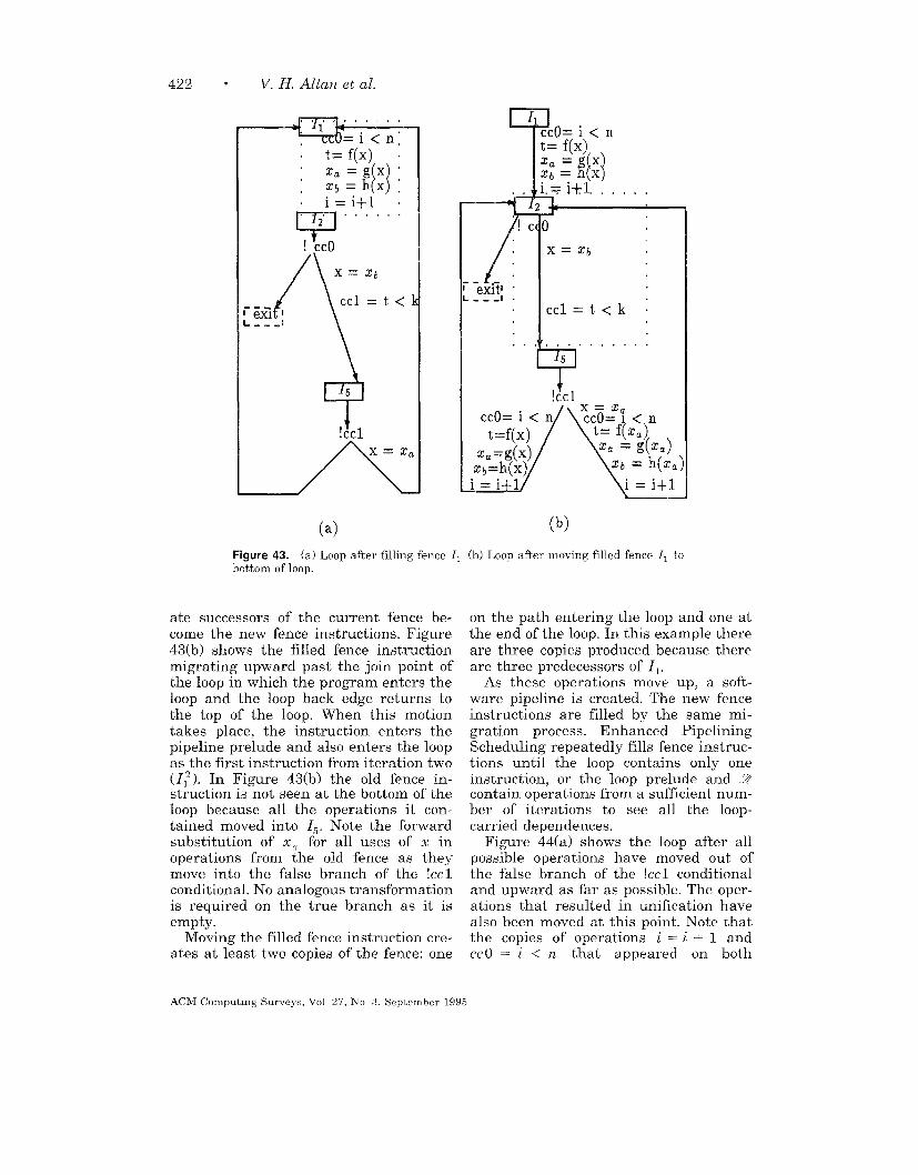
V. H. Allan et al.
t= f(x) :
[)
Za=gx “Xb=hx :i=i+l .
m’”””””
t<
L---/’Y(a)
Figure 43. (a) Loop after filling fence Ibottom of loop.
ate successors of the current fence be-come the new fence instructions. Figure43(b) shows the filled fence instructionmigrating upward past the join point ofthe loop in which the program enters theloop and the loop back edge returns tothe top of the loop. When this motiontakes place, the instruction enters thepipeline prelude and also enters the loopas the first instruction from iteration two
(l: ). In Figure 43(b) the old fence in-struction is not seen at the bottom of theloop because all the operations it con-tained moved into Is. Note the forwardsubstitution of x. for all uses of x inoperations from the old fence as theymove into the false branch of the !CC1conditional, No analogous transformationis required on the true branch as it isempty.
Moving the filled fence instruction cre-ates at least two copies of the fence: one
L
. .
7‘! ,
‘em-i :---
. .
1
X=xb
ccl=t<k .
. . . . . . ..!.
?
5
t!yl
Ax=x~
CCO= i < n CCO= 1 < n
t=f[x) t= f(xa)x~
Xa=g(x)= g(za)
zb=h(x) xb = h(L?a
i=il i = i+l
(b)
(b) Loop after moving filled fence II to
on the path entering the loop and one atthe end of the loop. In this example thereare three copies produced because thereare three predecessors of 11,
As these operations move up, a soft-ware pipeline is created. The new fenceinstructions are filled by the same mi-gration process. Enhanced PipeliningScheduling repeatedly fills fence instruc-tions until the loop contains only oneinstruction, or the loop prelude and %contain operations from a sufficient num-ber of iterations to see all the loop-carried dependence.
Figure 44(a) shows the loop after allpossible operations have moved out ofthe false branch of the !CC1 conditionaland upward as far as possible. The oper-ations that resulted in unification havealso been moved at this point. Note thatthe copies of operations i = i + 1 andCCO = i < n that appeared on both
ACM Computmg Sur\,eys, Vol 27, No .3, September 1995

Software Pipelining “ 423
I I [CCO= i < n
t= f(x)Za = g(x)
z~ = h(x)i = i+l
—12
:!co
/q
X=xb
ccl=t<k :
ccO=i<n~<t , : t = f(za) :--- J“
Zc = g(xa) .
‘+Xb = h(z. ) :
i=i+l 1.,.
“I’’””””””
!Ccl
-__QILt=f(x
Za=g(x) x=x~x~ = xc
xb=h X—
(a)
TI
cc=i<nt= f(x)
f[ 1
x—xX;z x
+
/
I1
i
X=Zb
h ccl=t<ki CCO= i < n
--. 1;?Xlt ,, t = f(xa)--- 1
1 Zc = g(za)I1 ~b = h(za)11 i = i+lt8 ta =f(xb)I
X~ = g(~b;11
‘$e = h(xb’I
I1,------
G------- .
t!Ccl
,---i1II1I1I1I1I1I111I11#11Ii111Ii1
. .
(b)
Figure 44. (a) Loop after migrating from false branch of the !CC1 conditional. (b) Loop after filling
branches of the condition !cc1, are eachmerged into a single operation as they
move past the branch point. Note also
that x. has been renamed x, as it movespast the use of x. that is assigned to x.
Figure 44(b) shows the loop after thefence instruction Iz has been filled. Fig-
ure 45 shows the final pipelined loop. Z
in this example is only one tree instruc-tion. Enhanced Pipeline Schedulingstarts with a large loop and reduces it insize as the pipelining proceeds. As theloop is always valid, the algorithm onlyiterates until the loop does not shrink insize. This occurs when the loop contains
only one instruction or when all loop-
carried dependence have been seen.The copy operations to x appear to be
redundant in % as x is never used. Thecopies to x are needed because x is liveon exit from the loop. Note that the oper-
ations originally assigned to x are now
executed speculatively and their resultsplaced in renamed copies of x. The copyoperations to x ensure the correct valueis assigned to x on loop termination. Theresulting loop is the pipelined loop body,
and the prelude and postlude are gener-ated automatically by the code duplica-
tion that occurs when operations are
ACM Computmg Surveys, Vol 27, No 3, September 1995

424 . V. H. Allan et al.
XII
ccO= i < n
t= f(x)
z= = g(x)
~b = h(x)
i = i+l
Iz
! Cco
/exit
!Ccl
,~\co
/i ‘eki - iL ---- J
Figure 45. Final pipelined loop
ACM Computmg Surveys, Vol 27, No 3, September 1995

Software Pipelining “ 425
m01: a[i] = b[i]/2
OZ : c[i] = a[i] + 2
03:d[i]=z+iI
04: if ccl
D
04 ; if ccl
/Exit
U ~ }
IZ
Oz:ci=a[i]+2 02:ci=a[i]+203:di=z+i H03:di =z+i
----[ 73~<it~ -~ ~ t t
i73 iL -- J
Figure 46. Example of copying operations to both branches of a moved branch operation
moved in the CFG. This pipeline has nopostlude because the exit branch nevermoves past other operations of the loop.
The postlude is generated when theconditional branch operation of the exittest is moved upward past code in theloop. When the branch is moved, anyoperations it moves past must appear onboth branches, resulting in the looppostlude. For example, Figure 46 showspart of a CFG before and after the branchoperation OL is moved to II. Note that Ozand OS must be copied to the exit tobecome part of the postlude branch asthey are executed regardless of the out-come of the conditional branch in theoriginal loop. The pipeline postlude withEnhanced Pipeline Scheduling is typi-cally small due to the renaming.
4.4 Redlucing Code Expansion
Enhanced Pipeline Scheduling places arestriction on the movement of opera-tions out of a filled fence to reduce thecode expansion that occurs because of thecopying of operations to both predeces-sors of a node, Operations are allowed tomove out of a filled fence instruction onlyif all the operations can move, but oncethe operations have moved out of a filledfence instruction, they are free to moveindependently of each other. Without this
requirement, given a node with twopredecessors, it is possible that code mo-tion would generate two versions of thenode without any execution time benefit,However, this restriction can result inaccepting a local minimum rather thanachieving the global minimum. En-
hanced Pipeline Scheduling does not havean optimal 11 value that it is trying toachieve, but stops when no further im-provements are seen.
Figure 47 shows an example of this
code duplication. When moving opera-tions from Is, OA can move to Iz whenforward substitution is used to collapsethe true dependence, but 04 cannot moveto the other predecessor of Is. The opera-tion 05 cannot move to either predeces-
sor of Is. If code motion is allowed inwhich operations of Is are allowed tomove independently, two copies of 1~ areneeded, one containing both OA and 05,
and the other containing only 05. If Is isa filled fence, this type of code duplica-tion would be prevented, as both OA and05 would have to move out of Is for anymovement to occur. Code duplication isexpensive, therefore Enhanced PipelineScheduling tries to reduce it.
In an improvement of Enhanced Pipe-line Scheduling, Nakatani and Ebcio~lu[1990] introduce a windowing technique
ACM Computmg Surveys, Vol 27, No 3, September 1995

426 * V. H. Allan et al.
Ol:x
02:
II1
IzI
= c[i]
y = d[i]
I
mII
04: a[x] = x/2
05: b[y]=z*5
+~----,1141L ---- J
‘u’
7)’01: z = c[i] 03:X=2
Oz : y = d[i]OZ : y = d[i]
OA. : a[z] = ,2/2
Is Is.
OA : a[z] = x/2 05: b[y]=z*5
05: b[y]=z*5
r--l
I 14 tL ---- J
Figure 47. Example of code duphcatlon
designed to reduce code expansion. When the work due to finding more parallelismEnhanced Pipeline Scheduling produces than can be utilized, they recommend
a pipeline assuming infinite resources, that the movement of operations be al-the instructions can become extremely lowed only within a given number of in-large, as renaming and forward substitu- structions (termed the window size) fromtion are repeatedly removing movement the current fence instruction. The win-blocking dependence. In order to reduce dow size can be set to a value that gives
AC’M Computmg Surve\,s, Vol 27, No 3, September 1995

Software ?ipelining “ 427
Table 6. Comparison of Algorithms
Lam Path Pred EMS Perfect Petri Vegdahl EPS
Fractional Rates no no no yes yes yes no
dif >1 yes yes yes yes yes yes yes nomin > 1 yes yes yes yes yes dummy dummy dummy
Resource Constraints yes no yes yes yes yes np np
Complexity poly poly poly 2’ poly poly 2“ poly
Code Expansion yes no no yes yes yes yes yes
Limited Rate yes yes yes yes no yes no yes
Leading Chain Problem no no no no yes no no no
E
Regular yes yes yes yes no no yes noKernel Recognition no no no no yes yes yes noModulo yes yes yes yes no no no no
good results for a particular application,A disadvantage of this technique is thatit can limit the number of iterations exe-cuting concurrently within X. When thewindow size is small, new operations fromfuture iterations are not within themovement window until several fence in-structions have been filled, thus slowingdown the rate at which they can migrateback up to the current fence instruction.
5. SUMhflARY
Table 6 summarizes the attributes of thevarious algorithms. The column, Path,represents Zaky’s path algebra algo-rithm. Pred represents the various predi-cated modulo scheduling algorithms.Perfect represents Aiken and Nicolau’sPerfect Pipelining. EPS represents En-hanced Pipeline Scheduling.
The table is divided into sections. The
UPPer ~ec~on shows factors that influ_ence efficiency of the target code pro-duced or the practicality of the algo-rithm. The middle section shows factorsthat influence the code size or compiletime. The bottom section lists attributesthat are descriptive in nature and do notaffect the efficiency of the code produced
or the generality of the algorithm, butmay help to classify the algorithms. Thistable is extremely useful not only in de-termining the best algorithms, but in
suggesting possible modifications to en-hance their capabilities.
The row labeled Fractional Rates indi-cates whether the algorithm achievesfractional initiation intervals withouthaving to replicate before scheduling. Allalgorithms can achieve fractional initia-tion intervals with replication, but sufferfrom the inability to decide easily on anappropriate replication factor.
All algorithms either address rnin
times of greater than 1 as an integral
part of the technique or introduce dummynodes to remove the occurrences. Difvalues greater than 1 are handled by allalgorithms except EPS which must repli-cate before scheduling to remove the oc-currences. All algorithms deal with gen-eral resource constraints except forZaky’s path algorithm. This is a seriouslimitation of Zaky’s algorithm. Resourceconstraints can be expressed by a limiton the number of functional units, a con-flict graph, or a resource vector of hetero-geneous resource requirements.
All methods handle irregular persis-tent resources except for Path (which ig-nores resource constraints) and thosemarked with np, which deal with non-persistent resources only.
Most of the algorithms have complex-ity 0( n3 ) or 0( n ~). However, Vegdahl’salgorithm is 0(2”) and is thus impracti-cal for even moderate sized problems.
ACM Computmg Surveys, Vol 27, No 3, September 1995

428 e V. H. Allan et al.
EMS has a worst case complexity of O(2 n )resulting from the exponential code ex-plosion, but such cases are rare.
Code expansion refers to the increasein code size caused by the same operationbeing repeated multiple times in theschedule (not counting prelude andpostlude). Any method that achievesfractional rate does so by incurring codeexpansion. Lam’s code expansion comesfrom scheduling operations that are notin branches with both versions of thebranch code and from modulo variableexpansion to eliminate loop-carried an-tidependences. The hardware support forpredicated modulo scheduling eliminatesthis code expansion. The transforma-tions EPS uses to reduce the length ofcyclic dependence also introduces codeexpansion.
Limited Rate indicates whether the al-gorithm uses the idea of a target 11 inmaking decisions. All modulo methodsbegin with a lower bound on the II inorder to save effort. In addition, becausea single copy of each operation exists inthe kernel, the rate is automatically lim-ited by 11. Kernel recognition algorithmsoften lack the ability to control the greed-iness in initiating iterations possibly re-sulting in greater compilation time,longer initiation intervals (greater execu-tion time), and greater span (increasedlength of prelude and postlude). The Petrinet algorithm achieves this limited ratevia the pacemaker (but this is an en-hancement to the algorithm rather thanan integral feature). In Perfect, rate isindirectly limited by setting the maxi-mum span of a single instruction as newoperations cannot execute if the set spanis exceeded. Vegdahl is exhaustive andsearches for all schedules, but alteringthe algorithm to limit the rate of execu-tion would greatly reduce the compiletime. In EPS, a limited rate does notexist per se, but the rate is limited by thenumber of times an operation is movedpast the back edge or the window size.
The Leading Chain Problem refers tothe problem that some algorithms experi-ence when there are one or more nodesthat are not successors of operations in
the critical cycle. A leading chain oftencreates problems in algorithms without ameasured rate as they are uncon-strained. Perfect solves the leading chainproblem by delaying operations when itis evident they are executing at differentrates.
It is possible for all methods to han-dle predicates within the loop when if-conversion is used. Only EPS is capableof achieving different II on each branchof a predicate. Lam schedules subprob-lems before combining. EPS and Perfectare transformation based. Petri andPath both can perform transformationsprior to scheduling to improve pipeliningresults.
The row labeled Regular indicateswhether an operation in the prelude orpostlude is executed at the same intervalas it is while executing the kernel. Inas-much as Vegdahl’s method does not spec-ify how the prelude and postlude are gen-erated, we assume a regular schedule isproduced. A regular schedule can be bothan advantage and a disadvantage. Be-cause the prelude and postlude executejust like the kernel (only with some oper-ations omitted), predicated execution canmake kernel-only code possible. How-ever, as some operations are omitted,separate scheduling of prelude andpostlude may be more efficient. This isa minor point as the conversion betweena regular schedule and an irregularschedule (and vice versa) is a trivialtransformation.
Most of the algorithms are either mod-U1O or kernel recognition, but EPS isneither.
5.1 Modulo Scheduling Algorithms
Rather than waiting for a pattern to form,modulo techniques analyze the DDG andcreate a desirable schedule. The tightcoupling of scheduling and pipeliningconstraints results in a pipeline that isnear optimal. The ability to adjust thescheduling technique to control registerpressure or prioritize by various at-tributes gives great flexibility. The regu-lar pipeline that is produced simplifies
ACM Computmg Surveys, Vol 27, No 3, September 1995

Software Pipelining “ 429
the formation of the prelude, kernel, andpostlude. With the replication suggested,fractional rates can be achieved [Jones1991]. The trial-and-error approach offinding the achievable 11 increases thecompile time, but no software pipeliningalgorithm has a tight bound on compiletime.
Zaky [1989] uses a technique that pro-duces results very similar to other mod-U1O scheduling techniques, but uses pathalgebra as a framework. Zaky’s algo-rithm is impractical as it cannot handleresource constraints, but is important be-cause of the elegant way it formulatesand solves the problem. Because of theconcise algorithm, this technique pro-vides an excellent conceptual model.
The modulo scheduling techniqueshave continued to improve by usinghardware support to reduce code expan-sion and allow tighter schedules by theuse of rotating register files. These meth-ods represent an excellent choice for soft-ware pi pelining, their only drawback be-ing that fractional rates are not achievedwithout replication before scheduling.
5.2 Perfect Pipelining
Perfect Pipelining is important from anhistorical perspective due to the early
work in exploration of pipelining involv-ing branches within the body of the loop.Unification is an important addition toearlier global code motion techniques.
Conceptually, Perfect Pipelining has anadvantage in that it is not forced to con-sider al 1 paths through the loop simulta-neously. In other words, various pathsthrough the loop are able to achieve adifferent initiation interval. The fre-quency of achieving optimal overall re-sults is hampered by the ad hoc nature ofthe scheduling.
The main disadvantage of PerfectPipelining is the difficulty of determiningwhen two nodes are functionally equiva-lent. Other problems include the genera-tion of loops that contain more copies ofthe original iteration than needed andthe need to help the pattern develop.
5.3 Petri Net Model
The Petri net model is another excellentchoice for software pipelining due to its
strong mathematical orientation andflexibility in adapting to a wide variety ofconstraints. General reservation modelspose no problem for this adaptablemethod. It produces excellent schedules,its only drawback being the need tosearch for a pattern.
5.4 Vegdahl
Vegdahl’s method is an interesting theo-retical tool. Because of its exponentialcomplexity, it is not a practical tech-nique, but serves as an “optimal” forsmall code size. The method could beadapted for use with persistent re-sources, but would significantly increasethe run time. Perhaps Vegdahl’s methodcould be used in combination with othertechniques. For example, if moduloscheduling was used to determine spanand 11, Vegdahl’s exhaustive techniquecould be greatly restricted to explore so-lutions with span and 11 slightly better
than the achieved. A parallel implemen-tation of a greatly reduced search spacecould make the algorithm reasonable fora broader class of problems.
5.5 Enhanced Pipeline Scheduling
Enhanced Pipeline Scheduling is unique.Not only does it deal with multiblockloops, but it always maintains a legalloop structure rather than trying torebuild the loop. Enhanced PipelineScheduling handles general loops. Al-though renaming and forward substi-tution have been utilized for years, thedegree to which they have been success-fully employed in this technique is note-worthy.
Enhanced Pipeline Scheduling has sev-eral advantages over Perfect Pipelining.The algorithm increases the speed of con-vergence by retaining the loop constructand reducing the resulting code size.These techniques can also cause prob-
ACM Computmg Surveys, Vol. 27, No 3, September 1995
430 “ V. H. Allan et al.
lems, as prematurely forcing operationsto remain together can restrict the paral-lelism. These disadvantages are lessenedif a majority of the loop dependence canbe removed by the automatic renamingand combining. The most serious draw-back is the unsuitability of the methodfor use with persistent resources. Be-cause instructions are inserted or re-moved during the scheduling, persistentresources (that require a fixed set of re-sources a given offset from instructioninitiation) cannot be accommodated.Fractional rates are not achieved.
6. CONCLUSIONS ANEI FUTURE WORK
Software pipelining is an effective tech-nique for extracting parallelism fromloops that thwart attempts to vectorizeor divide the work across processors.Although the speedup is modest, itshould be noted that software pipeliningsucceeds where other methods fail andcan be applied after other techniqueshave extracted coarse grain parallelism.The variety of architectures benefitingfrom software pipelining underscores itsimportance.
Although an NP-complete schedulingproblem, software pipelining has numer-ous effective heuristics that have beendeveloped. Both resource conflicts andcyclic dependence produce a lower boundon the initiation interval. Such lower
bounds can be computed in polynomialtime. In considering algorithmic featuressuch as low complexity, ability to dealwith conditionals, accommodation of re-source conflicts, and achievement of frac-tional initiation intervals, the currentn~ethods have various degrees of success.
Some researchers are applying artifi-cial intelligence techniques to the prob-lem of software pipelining. Beaty [ 1991]uses genetic algorithms for instructionscheduling. O’Neill [1994] and Allan andO’Neill [1994] use genetic algorithms andsimulated annealing to solve the problemof software pipelining. In the future, weexpect to see more improvements in theapplication of artificial intelligence tech-niques to scheduling problems.
ACKNOWLEDGMENTS
The authors would Ilkc to thank B R Rau for h]s
insight Into the history of modulo scheduling and
hls pamstakmg attention to the detads of this pa
per. Thanks to the anonymous referees, The quallty
of the paper has been tremendously Improved by
them comments This work was supported m part
by the Nat]onal Science Foundation grants CDA-
9100788 and IRI-S901175
REFERENCES
AHO, A V, Sirmu, R, AND ULLMMV, J D 1988Cnmpilcr~ Prlnclple~, Techniques, and Tools
Addison-Wesley, Reading, MA
ATKEN, A 1988 CompactIon-based parallehza-
tlon Cornell Umverslty, Dept of Computer Sci-ence, Ph D Thesm. Ithaca, NY
AIKEN, A. AND NLCOLiIU, A 1988a. A developmentenvu-onment for horizontal microcode IEEETrams Softw. Eng. 14, 5 (May), 584-594
AI%N, A AND NICOL~L~, A 1988b Optimal loopparallehzatlon In Prowedzngs of the SIGPLAN
’88 Conference on Programming Language De-
sign and Implementation (Atlanta, GA. June),308-317
A1hEN, A. AND NICOLAL, A, 1988c. Perfectplpehmng. A new loop optlmlzatlon techmque,
In Proceedings of the 1988 European Sympo-
szum on Programming. Springer Verlag Lec-ture Notes zn Computer Science, #300 (Atlanta,GA, March), 221-235
AIKEN, A ANII NICOLP.LT, A 1990 A reallsticresource-constrained software plpehrnng algo-rithm Tech Rep RJ 7743, IBM Research Dlvi-
slon, San Jose, CA, October
ALLAN, V, H, AND O’NEILL, M. R, 1994. Software
plpehnmg: A genetic algorithm approach, InPACT 94 (Montreal, Canada, Aug. 23–26).North-Holland, Amsterdam, 311–314
AT LAN, V H , RAJAGOPALAN. M , AND LEh, R M
1993. Software plpehmng Petri net pace-maker In Working Con ferpnce on Arch ztectures
and Cornpzlat[arz Techniques for Fzne andMedzam Grain Parallelzsrn (Orlando, FL, Jan
20–22) North-Holland, Amsterdam, 15–26
BANERJMi, U , SHFX, S , KUCK, D J., .LNn TOWLE.RA 1979 Time and parallel pr.ccswmbounds for Fortran-hke loops. IEEE !l’ransComput C-28, 9 (Sept ), 660-670
BEAT~, S, J. 1991, InstructIon scbeduhng using
genetic algorithms. Colorado State Umverslty,Fort Colhns, CO, Ph D Thesm,
BWK. G. R , Y~N, D W L , W~ ANDERS lN, T L
1993 The C’ydra 5 mimcomputer Architec-ture and implementation In J Supercomput(May), 143-180
BRETERNITZ. M,. JR. 1991, Architecture synthesisof high-perforrnance apphcatlon-speclflc ~roces-som Carnegie Mellon Universlt~,, Pittsburgh,PA, Ph D Thesis
ACM Computing Surve>~, Vol 27, No d, September 1995

Software Pipelining “ 431
CHANDY, K. M. AND KESSELMAN, C. 1991 Parallelprogramming in 2001. IEEE Softzo. 8, 6 (Nov.),
11-20.
DAVIZMON, E. S. 1971, The design and control of
pipehned function generators, In F’mceedmgsof the 1971 International IEEE Conference on
S.vsterns, Netzuorks, and Computers (Oaxtepec,Mexico, Jan.), 19-21.
DEHNERT, J. C., HSCT, P, Y.-T., AND BRATT, J, P.
1989. Overlapped loop support m the Cydra-5.In Proceedings of the Thzrd International Com
ference on Architectural Support for Progrant-nung Languages and Operatzng Systems (Bos-
ton, MA, April), 26-38.
D~HNERT, J. C. AND TOWLE, R, A. 1993. Compil-
ing for the C ydra-5. In J. Supercomput. (May)j
181-228.
E~c10t2Lu, K. 1987. A compilation technique for
software pipelining of loops with conditionaljumps. In Proceedings of the 20th Micropro-
gramming Workshop ( MZCRO-20) (Colorado
Springs, CO, Dec.), 69-79
EBCIOi3LU, K. AND NAKATANI, T. 1990. A new com-pdation techmque for parallelizing loops with
unpredictable branches on a VLIW architec-ture. In Languages and Gompders for ParallelComputmg, D. Gelernter, Ed,, MIT Press.
Cambridge, MA, 213-229.
FERRANTE, J,, OTTENSTEIN, K. J., AND WARREN, J. D.
1987. The program dependence graph and its
use m optimization. ACM Trans. Program.Lang. Syst. 9, 3 (July), 319-349.
FISHER, J. 1981. Trace scheduling: A technique
for global microcode compaction. IEEE Trans.Comput. C-30, 7 (July), 478-490.
FRTZUD~NMIRG~R, S. M., GROSS, T. R., AND LOWNEY,
P. G. 1994. Avoidance and suppression of
compensation code in a trace scheduler ACMTrans. Program. Lang. Syst. 16, 4 (July),1156-1214.
GAO, G. R., WONG, W.-B., AND NING, Q. 1991a. Atimed Petri-net model for fine-grain loopscheduling. In Proceedings of the ACM SIG-PLAN ’91 Conference on Programmmg Lan-
guage Design and Implementation (June26-28), 204-218.
GAO, G. R., WONG, W.-B., AND NING, Q. 1991b. Atimed Petri-net model for tine-gram loop
scheduhng. Tech. Rep. ACAPS Technical Memo18, School of Computer Science, McGdl Univer-
sity, Montreal, Canada, H3A 2A7, January.
GOWNDARAJAN, R., ALTMAN, E. R., AND GAO, G. R.1994, Minimizing register requirements un-
der resource constrained rate-optimal softwarepipclining. In Proceedings of the 27th AnnualInternational Symposium on Micz-oarchitectuz-e,to appear.
Hsu, P. Y. T. 1986. Highly concurrent scalar
processing. University of Ilhnois, Urbana-Champaign, Urbana-Champaign, IL. Ph.D.Thesis.
Hsu, P. Y T. AND DAVIDSON, E. S. 1986. Highly
concurrent scalar processing. In Proceedings of
the Thirteenth Annual In ternatlonal Sympo-
.wum on Computer Architecture, 386–395.
HUFF, R. A. 1993. Lifetime-sensitive moduloscheduling. In Conference Record of SIGPLANProgrammmg Language and Desgn Implenten -tat~on (Albuquerque, NM., June). ACM, NewYork, 258-267.
JONES, R, B. 1991. Constrained software pipelin-ing. Utah State University, Dept. of ComputerScience, Logan, UT, Master’s Thesis, Sept.
JONES, R. B. AND ALLAN, V. H. 1990. Softwareplpelining: A comparison and improvement. InProceedings of the 23rd Znternatzonal Sympo-
swm and Workshop on Mlcroprogrammmg andMzcroarchztecture (MICRO-23 ) (Orlando, FL,
Nov. 27-29). IEEE Computer Society Press,46-56.
KUCK, D. J. AND PADUA, D. A. 1979. High-speed
multiprocessors and their compilers. In Pro-ceedings of the 1979 Internatzmzal Conference
on Parallel Processing, 5–16.
LAM, M. S. 1988. Software pipelining: An effec-tive scheduhng technique for VLIW machines.In Proceedings of the SIGPLAN ’88 Conference
on Programnung Language DesLgn and Imple -rnentatzon (Atlanta, GA, June), 318–328.
LAM, M. S. 1987. A systolic array optimizing
compiler. Carnegie Mellon University, Dept. ofComputer Science, Pittsburgh, PA, Ph.D. The-sis.
MAHLKE, S, A., LIN, D. C., CHEN, W. Y., HANK, R. E.,AND BRINGMANN, R. A. 1992. Effectwe com-
piler support for predicated execution using thehyperblock. In Proceedings of the 25th AnnualInternational Symposwm on Mlcroarchitecture
(MICRO-25) (Portland, OR, Dec. 1-4), 45-54.
MATETI, P. AND DEO, N. 1976. On algorithms for
enumerating all circuits of a graph. SZAM J.Comput. 5, 1,990-999.
NAKATANI, T. AND EBCIO~LU, K. 1990. Using alookahead window in compaction-based paral-lehzing compder. In Proceedings of the 23rd
MLcroprogrammlng Workshop ( MZCRO-23)
(Orlando, FL, Nov.). IEEE Computer SocietyPress, 57-68.
NAKATANI, T. AND EBCIOGLU, K. 1989. “Combin-ing” as a compilation technique for VLIW ar-chitectures. In Proceedings of the 22nd Micro-programming Workshop ( MICRO-22) (Dublin,Ireland, Aug.), ACM, New York, 43-55.
NICOLAU, A. AND POTASMAN, R, 1990. An envmon-ment for the development of microcode forpipelined architectures. In Proceedings of the23rd SymposizLm and Workshop on Micropro-gramming and Microarchitectuz-e (Orlando, FL,Nov.), 69-79.
O’NEILL, M, R. 1994. Software plpelining withstochastic search algorithms. Utah State Uni-
versity. Dept. of Computer Science, Logan, UT,Master’s Thesis.
ACM Computmg Surveys. Vol 27, No 3. September 1995

432 ● V. H. Allanet al.
RAJii~o~.ALAN, M. AND ALLAN, V.H, 1994. Speclfl-catlon of software pipehmng using Petri netsInt J. Parallel Process 3, 22, 279–307.
RAIT, B. R 1994 Iterative modulo scheduhng An
algorithm for software plpehned loops In Pro-
ceedings of Mw-o-27, The 27th Annual Interna -tmnal Sympostum on Mmroarchu!ecture (SanJose, CA, Nov 29-Dee. 2) ACM, New York.
63-74
RAU, B. R. AND FISHER, J. A. 1993. Instructlon-level parallel processing History, overview, and
perspective. J. Supercomputmg 7, 9-50.
RAU, B. R., LEE. M , TIRUMIiLM, P P , ANDSCHLANSKER, M S 1992 Register allocation
for modukz scheduled loops Strate@es, algo-rithms, and heuristics. In Proceedings of theACM SIGPLAN ’92 Conference on Program-mrng Language Design and Implementchon
(San Francisco, CA, June ), ACM, New York,283-299
RAU, B R., SCHLANSKSR, M S , m~ TIRUMALAI, P P1992 Code generation schema for modulo
scheduled loops. In Proceedings of Mzcro-25,The 25th Annual International Sjmposzzzm on
Microarch/tecturt (Dec.) IEEE Computer Soci-
ety Pres>, 158–169
RAU, B R., YEN, D. W L , YEN, W.. AND TOWLE,R. A. 1989. The Cydra 5 departmental su-
percomputer: Design phdosophles, decmlons,and trade-offs IEEE Cornput. (Jan.), 12–25.
RAU, B. R. AND GLAESER, C. D. 1981 Somescheduling techniques and an easily schedula-ble horizontal architecture for high perfor-mance scientific computmg In Proceedings of
the Fourteenth Annual Workshop of Micropro-gramming (Ott ), 183-198
RAU, B. R., GLAESER, C. D., AND GREENt~7ALT, E. M.198’2, Architectural support for the efficient
generation of code for horizontal architectures.In Proceedings of the Symposl urn on Arch ~tec-tural Sapport for Progrccmmzng Languages and
Operating Systems (March), 96-99.
SMIrH, H F 1987 Data Structures Form and
Fanctzon Harcourt Brace Jovanovich, SanDiego, CA
Su, B., DING, S., WANG, J,, AND XIA, J, 1987.GURPR—A method for global software plpe-lining. In Proceedings of the 20th Mzcropro-grammmg Workshop ( MIC’RO-20) (ColoradoSprings, CO, Dee ), 97-105.
Su, B , DING, S., AND Xm, J. 1986. URPR—Ancxtenslon of URCR for software plpehm ng. InProceedings of the l%h Mlcroprogramm zngWorkshop ( MICRO-19) (New York, Oct.),104-108.
TARJAN, R 1972 Depth-first search and linear
graph algorithms. SI.4M J, C’omput. 1, 2 (June),
146-160
TIERNAN, J C. 1970. An efficient search algo-
rlthm to find the elementary circuits of a graph.
Commun ACM 13, 1, 722-726
TIRUMALAI, P., LEE, M , AND SCHLANSKER, M S.
1990 Parallelization of loops with exits on
p,pehned architectures In Proceedings of
SuperComputmg ’90 (Amsterdam, Nov ), ACM,New York, 200-212
TOKCMW, M , TAMURA, E., TAK.A\E, K, AND TAMARU,
K. 1977 An approach to microprogram opti-
mization considering resource occupancy and
instruction formats In Proceedr ngs of the
10th Annual Workshop on M[croprogrumnung
(Niagara Falls, NY, Nov.), 92-108
VEGI)AHL, S R. 1992 A dynamic-programming
technique for compacting loops In Proceeduzgsthe 25th Annual International Symposium on
Mzcroarclzztecture ( MICRO-25) (Portland, OR,Dec ) IEEE Computer Society Press, 180-188
VEC,D.AHL, S R 1982 Local code generation and
compaction in optlmlzmg microcode compders
Carnegie-Mellon Umversity. Dept of Computer
Science, Pittsburgh, PA, Ph D Thesis
WARTER, N J., HmB, G. E , AND Bocmwms, J. W
1992 Enhanced modulo scheduling for loops
with conditional branches In Proceedings of
the 25th Annual International Symposzum on
Mzcroarchztecture (MICRO-25) (Portland, OR,Dec 1–4), IEEE Computer Society Press,
170-179
WARTER, N. J , MAHLKR, S A, Hwu, W. M W., AND
RAU, B R 1993 Reverse If-conversion InPLDI (Albuquerque, NM, June) ACM, New
York, 290-299
WOLFE, M. J. 1990. Tzny—A Loop R.estructuruzg
Tool, User Manual Oregon Graduate Institute
of Science and Technology, Beaverton, OR.
WOLFE, M J 1989 Optzmzzzng Supercompders
for Supercomputers MIT Press, Cambridge,
MA.
WooD, W, G. 1979. Global optlmlzatmn of micro-programs through modular control constructs
In proceedings of the 12th Mlcroprogramm lng
Workshop (MICRO-12) (Hershey, PA, Nov.),1-6.
ZAzm, A. M. 1989. Efi’iclent stat]c scheduhng of
loops on synchronous multiprocessors, Ohio
State University, Dept. of Computer and Infor-mation Science, Columbus, OH, Ph.D. Thesis.
ZIMA. H, AND CHAPMAN, B. 1991. Supercornpllers
for Parallel and Vector Computers ACM, NewYork
Received November 1993, rewed version received February 1995, final revlslon accepted July 1995,
ACM Computjng Surveys, Vol 27, No 3, September lq95


![Pipelining & Parallel Processing - ics.kaist.ac.krics.kaist.ac.kr/ee878_2018f/[EE878]3 Pipelining and Parallel Processing.pdf · Pipelining processing By using pipelining latches](https://img.dokumen.tips/doc/110x75/5d40e26d88c99391748d47fb/pipelining-parallel-processing-icskaistackricskaistackree8782018fee8783.jpg)