SOEPpaperson Multidisciplinary Panel Data Research

Well-Being in Germany: What Explains the Regional Variation?Johannes Vatter

435 201

2SOEP — The German Socio-Economic Panel Study at DIW Berlin 435-2012

SOEPpapers on Multidisciplinary Panel Data Research at DIW Berlin This series presents research findings based either directly on data from the German Socio-Economic Panel Study (SOEP) or using SOEP data as part of an internationally comparable data set (e.g. CNEF, ECHP, LIS, LWS, CHER/PACO). SOEP is a truly multidisciplinary household panel study covering a wide range of social and behavioral sciences: economics, sociology, psychology, survey methodology, econometrics and applied statistics, educational science, political science, public health, behavioral genetics, demography, geography, and sport science. The decision to publish a submission in SOEPpapers is made by a board of editors chosen by the DIW Berlin to represent the wide range of disciplines covered by SOEP. There is no external referee process and papers are either accepted or rejected without revision. Papers appear in this series as works in progress and may also appear elsewhere. They often represent preliminary studies and are circulated to encourage discussion. Citation of such a paper should account for its provisional character. A revised version may be requested from the author directly. Any opinions expressed in this series are those of the author(s) and not those of DIW Berlin. Research disseminated by DIW Berlin may include views on public policy issues, but the institute itself takes no institutional policy positions. The SOEPpapers are available at http://www.diw.de/soeppapers Editors: Jürgen Schupp (Sociology, Vice Dean DIW Graduate Center) Gert G. Wagner (Social Sciences) Conchita D’Ambrosio (Public Economics) Denis Gerstorf (Psychology, DIW Research Professor) Elke Holst (Gender Studies) Frauke Kreuter (Survey Methodology, DIW Research Professor) Martin Kroh (Political Science and Survey Methodology) Frieder R. Lang (Psychology, DIW Research Professor) Henning Lohmann (Sociology, DIW Research Professor) Jörg-Peter Schräpler (Survey Methodology, DIW Research Professor) Thomas Siedler (Empirical Economics) C. Katharina Spieß (Empirical Economics and Educational Science)

ISSN: 1864-6689 (online)

German Socio-Economic Panel Study (SOEP) DIW Berlin Mohrenstrasse 58 10117 Berlin, Germany Contact: Uta Rahmann | soeppapers@diw.de

Well-Being in Germany: What Explains theRegional Variation?

Johannes Vatter∗

March 7, 2012

Abstract

This paper examines regional differences in subjective well-being (SWB)in Germany. Inferential statistics indicate a diminishing but still signifi-cant gap between East and West Germany, but also differing levels of SWBwithin both parts. The observed regional pattern of life satisfaction reflectsmacroeconomic fundamentals, where labor market conditions play a dom-inant role. Differing levels of GDP and economic growth have contributedrather indirectly to regional well-being such that the years since the Germanreunification can be considered as a period of joyless growth. In total, ap-proximately half of "satisfaction gap" between East and West Germany canbe attributed to differing macroeconomic conditions. Moreover, the effectsof unemployment and income differ in size between regions such that onecan assume increasing marginal disutility of unemployment. The compara-bly high levels of life satisfaction in Northern Germany are driven mostlyby couples and go along with significantly higher fertility rates. Overall,we conclude that comparisons of SWB within a single country provide validinformation.

JEL-Classification: R10, I31

Keywords: subjective well-being, regional disparities, unemployment, economicgrowth, fertility rate

∗Forschungszentrum Generationenvertärge (Research Center for Generational Contracts),Albert-Ludwigs-Universität Freiburg (Freiburg University), D-79085 Freiburg, Germany (Phone:+49-761-203-9236. Corresponding author: E-mail address: johannes.vatter@vwl-uni-freiburg.de).The author is grateful for helpful comments from Stefan Moog, Daniel Ehing, Klaus Kaier andMatthias Weber. All errors remain my own.

1

1 Introduction

Happiness is not just a popular topic for front-page stories. The vast moun-tain of economic literature on human well-being that has grown during thelast two decades (see, e.g., Kahneman and Krueger [2006], Blanchflower andOswald [2008] or Oswald and Wu [2010]) suggests that individuals’ subjec-tive well-being (subsequently referred to as SWB) provides credible informa-tion. Hence, happiness economics or – more precisely – evidence based onself-assessed life satisfaction is a promising approach to specify our understand-ing of utility, to update our welfare reporting standards and to complement thetraditional framework of revealed preferences (see Ng [2003]).

Analyses of reported life satisfaction are also highly recognized due to the on-going skepticism about the hitherto promises of further economic growth. Ba-sically, one can find two lines of critique with respect to GDP as a key welfareindicator and major policy objective. The first line of critique has been estab-lished by the influential remarks of Richard A. Easterlin on the relationshipbetween growth and well-being. Easterlins’ analyses suggest not just a smallbut no significant relation at all (see Easterlin [1974] and more recently Easter-lin [2005]). However, for developed societies this seeming paradox of a joylessmaterial growth can be widely explained by material repletion, increasing in-equality and the human ability to quickly adapt to higher levels of consumption(see, e.g., Lane [2000] or Clark et al. [2008]). A second line questions the com-patibility of economic growth and ecological sustainability and goes back to theearly 1970s and the Club of Rome.1 Although this critique rather is concernedabout the consequences of economic growth in the long run, it has also stressedthe importance of the question whether the GDP is a valid measure for todaysquality of life.

As a consequence of these debates, countless private and more and more pub-lic initiatives are searching for new ways to measure welfare in a more pre-cise and forward-looking way than it is done by the GDP.2 But serving bothkinds of requirements – measuring current well-being precisely and includingaspects of sustainability – seems to be an unsolvable task as it would includesubstantial trade-offs within one key indicator. One important subordinatedquestion is, however, whether data on SWB is really able to measure the cur-rent level of well-being of a nation (or region) validly. In fact, social scientistshave gained more and more confidence in using and interpreting data on SWB.Indeed. Many have come to the conclusion that these data could solve the prob-lem of how to measure welfare itself instead of using complicated indicators(see, e.g., Kahneman et al. [2004], Layard [2010] or Diener and Tov [2012]).Among several caveats of the idea of accounting national well-being by using

1More recently the main focus of this debate has shifted from the finiteness of natural resourcesto the aspects of climate change and the global distribution of resources.

2Probably the most recognized attempt to complement the GDP has been undergone by theCommission on the Measurement of Economic Performance and Social Progress which was as-signed by the French government. Additionally, the European Commission ("beyond gdp") and theOECD ("better life initiative") have become active in this field. And also in Germany an Enquete-Commission titled "Growth, Welfare, Quality of Life" ("Wachstum, Wohlstand, Lebensqualität") hasrecently been established in order to develop an alternative concept to measure the quality of lifethat enables politicians and the society as a whole to operate and decide on the basis of valid welfareindicators and without being short-sighted.

2

subjective information, a striking one has been the lack of international compa-rability. Whether an indicator is used or not, crucially depends on the questionwhether it is internationally or regionally comparable or not. If it is not certainthat country A is really doing better than country B, it is rather useless to searchfor root causes of different levels of well-being which in turn could serve as anevidence base for policy measures. This issue becomes even more delicate ifcountries or political unions such as the EU explicitly try to balance unequalliving conditions.

This paper discusses the applicability of self-assessed life satisfaction as an ad-ditional welfare indicator by focussing on regional differences within Germany.Thereby three major questions shall be answered: First, do regional mean val-ues of reported life satisfaction reflect real differences in well-being? Second,by how much can the regional variation be explained by established welfareindicators such as GDP or the unemployment rate? Third, what else contributesto the observed regional pattern of SWB within Germany? Finally, we also dis-cuss the question whether SWB might be a proper instrument to complementthe existing reporting systems and which determinants of national well-beingshould receive more attention.

The remainder of the article is as follows. Section 2 provides a short insight intorelated research. Section 3 discusses the database and provides some descrip-tive statistics. In Section 4, we show up to which point the regional variation ofSWB can be explained by macroeconomic fundamentals such as GDP and unem-ployment. Section 5 provides some additional explanations for the comparablylow levels of SWB in East Germany as well as for the ’nordic happiness puzzle’.Section 6 summarizes.

2 Related literature

Especially for developed countries the demand for adequate regional compar-isons on welfare has significantly increased during the past years. However,some authors are skeptical with respect to the validity of international compar-isons based on subjective information (e.g., Sachverständigenrat [2010]). Thearguments are manifold: Simple cross-country comparisons might become mis-leading due to different regional perceptions of the question (e.g., Wierzbicka[2005]). It can also be argued that regional aspiration levels are differing suchthat it comes to an unequal interpretation of the given answering scale. More-over, cultural differences and social norms can lead to special respond behav-iors, and therefore, cause additional biases (e.g., Vittersø et al. [2005]).

While most articles do not thoroughly discuss these pitfalls, some authors havestarted to examine cross-country panel data and included country fixed-effectsin order to avoid unobserved regional effects within cross-sectional observa-tions (see, e.g., DiTella et al. [2003], Helliwell [2003] or Alesina et al. [2004]).Cross-national surveys of this kind have helped to estimate the impact of differ-ent political constitutions, institutions or macroeconomic conditions on overalllife satisfaction without denying differences in mentality and cross-sectional bi-ases. Other authors like Kristensen and Johansson [2008] have stressed theseissues even more and use vignettes to control for cultural biases to receive more

3

valid, and therefore, comparable figures. Despite of such examples, a majorexplanation for the relatively incautious use of international (or interregional)data might be its plausible pattern. Among several international rankings ofwell-being the most serious ones are based on the Eurobarometer, the WorldValue Survey, the World Gallup Poll and the International Social Survey Pro-gram. These international sources strongly suggests that reported life satisfac-tion is rather determined by objective conditions and obvious cultural achieve-ments than by language, adopted aspiration levels or unobserved mentalities(see Diener and Klingelmann [2000], Veenhoven and Ehrhardt [1995], Dieneret al. [1995], Frey and Stutzer [2002], and Sacks et al. [2010]). In fact, alldata generally show significant correlations with objective life conditions suchas health standards or income.

However, while traditional welfare indicators such as the GDP are able to ex-plain large parts of the global variation in SWB, this is not necessarily the casefor the developed world. As on the individual level (see Layard et al. [2008]),several authors stress that additional income is becoming also less important oreven obsolete on an aggregated level (see, e.g., Lane [2000], Oswald [1997] orEasterlin [2005]). More recent research suggests, however, that higher levels ofeconomic output still raise reported well-being significantly even if many ma-terialistic needs have been satisfied already (Clark et al. [2008], Blanchflowerand Oswald [2004], and Shields and Price [2005]). In an ordered probit modelusing data from the Eurobarometer for 12 European countries, Di Tella et al.[2003] find significant effects for both the level as well as the fluctuation ofGDP. Helliwell [2003] explores regional differences among 14 industrial coun-tries by using the World Value Survey and finds decreasing but positive effects ofaggregated income as well. Significant and notable effects of GDP per capita arealso found by Stewart [2005]. Sacks et al. [2010] confirm the general findingthat marginal utility of GDP diminishes, however, they also argue that there arestill notable effects even in the highly developed world. Overall, GDP is foundto explain the international pattern of SWB (still) quite well, even within thedeveloped world.

The probably second most recognized welfare indicator – the unemploymentrate – and its impact on the overall life satisfaction of a society have been stud-ied extensively as well. Without controversy are the strong and durable effectsof unemployment on the individual level (see, e.g., Clark and Oswald [1994] orWinkelmann and Winkelmann [1995]). Aiming on the effects on the aggregatedlevel, DiTella et al. [2001] estimate the social welfare tradeoff between unem-ployment and inflation using a cross-country panel. After controlling for severalpersonal characteristics, country fixed effects, and year effects, they concludethat unemployment marginally leads to higher welfare losses compared to in-flation. Unemployment is also studied by DiTella et al. [2003] for 12 Europeancountries. Using data from 1975 to 1992, their results suggest that unemploy-ment has been less important than GDP when it comes to the regional variationof SWB.

Harder to grasp but also relevant for overall levels of SWB seems to be the de-gree of inequality within one country. Oishi et al. [2011], Rousseau [2009]as well as Böhnke and Kohler [2010] argue that rising income inequality is akey factor to understanding the moderate increase in SWB within many devel-oped countries. As a consequence, differing levels of inequality presumably also

4

explain parts of the international variation in SWB. In comparison to other influ-ential variables, however, the perception and impact of inequality probably varyconsiderably between nations (Alesina et al. [2004]). Furthermore, research onhappiness and inequality is not that voluminous due to the lack of long andcomparable cross-country panel data. Several authors also stress the relevanceof different kinds of social capital. For example, Helliwell [2003] finds a signifi-cant relationship between the level of communal responsibility of a society andthe level of life satisfaction. Bjørnskov [2006] emphasizes the different aspectsof social capital and argues that indicators of social trust are strongly relatedto life satisfaction. Overall, it can be stated that an increasing and significantshare of the international variation in SWB can be explained in a plausible waybased on a manifold set of objective variables. The listed examples provide justa selection of a large number of articles published during the last years.

In contrast to international comparisons, regional analyses of SWB within onecountry have the advantage that all regions (in most cases) share one languageand homogenous cultural traditions which reduces the potential of unobserv-able or just unobserved heterogeneity. On the other hand, differences in SWBobviously tend to be smaller, and therefore, more difficult to detect and to ex-plain statistically. Recent studies, however, have shown for example significanteffects of objective living conditions. Oswald and Wu [2010] provide evidencefor the US in which SWB goes along with a bundle of objective indicators forquality of life. Frey and Stutzer [2002] focus on the impact of institutionaldesign with cross-regional data from Switzerland. Luechinger [2011] providesevidence on the relationship of air quality and life satisfaction with data fromGerman Socio-oeconomic Panel (SOEP) and high-resolution SO2 data.

With respect to Germany, however, most articles have studied regional differ-ences on a descriptive level. Berlemann and Kemmesies [2004] reported re-gional aspects of well-being for Germany based on the Eurobaromenter. Maddi-son and Rehdanz [2007] argue that regional levels of SWB within Germanyare rapidly converging due to migration and the adjustment of rent prices.Bergheim [2008] analyses SOEP data on a high-resolution level and empha-sizes the correlation of fertility rates and life satisfaction. Easterlin and Plagnol[2008] focus on the evolution of SWB in East and West Germany after reunifi-cation. Raffelhüschen et al. [2011] compare the regional pattern of SWB withthose of several well-explored drivers of well-being and find unexpectedly highsatisfaction levels in northern regions. However, to my knowledge there hasbeen no study that explicitly analyzes the drivers of regional variation in SWBwithin Germany.

5

3 Database

3.1 Datasource

The following analyses are based on the German Socio-oeconomic Panel (subse-quently referred to as SOEP), a longitudinal survey that exists since 1984. Thequestion on overall life satisfaction – "Taken all things together, how satisfiedare you with life?" (Wie zufrieden sind sie, alles in allem, mit Ihrem Leben?)– is answered by choosing a level on an eleven-point-scale (ranging from "notsatisfied at all" = 0 to "absolutely satisfied" = 10). Besides this information thepanel contains a wide range of socio-economic variables on both individual andhousehold characteristics. The SOEP database has started for West Germanywith a sample of 12245 observations which has been to small to conduct ex-tensive regional analyses. Subsequently however, the number of observationshas increased due to added subsamples as well as data refreshments. Withmore than 24500, the largest number of observations was achieved in the year2000. In the following years the number has slightly decreased according topanel mortality. In the wave of the year 2009, which has been the one recentlyavailable, 18602 interviews have been conducted. All respondents are of age16 or older. The long time span of the panel, the considerable variety of socio-economic variables and the large number of observations have made the SOEPto one of the most frequently used datasets for exploring the evolution andcauses of subjective well-being (see Wagner et al. [2007]).

3.2 Regionalization

The SOEP is used for cross-regional analyses only rarely. This mainly has todo with the fact that the sample design is done in a way that the observa-tions are – accordingly weighted – representative for whole Germany but notnecessarily for smaller regions within Germany. Despite of the subsample forEast Germany that has been designed and added in 1990 in order to allowalso separated analyses for West and East, the possibility of drawing detailedcomparisons between single regions is limited due to the decreasing numberof observations per region. Nevertheless, the approximately 20.000 observa-tions that have been made each year since 2000 are spread over all parts ofGermany according to the density of the population. The data are collected ina way that the number of observations is proportional to the population of thefederal states (Bundesländer) and it reflects rural areas and agglomerations rep-resentatively. As the addresses of the respondents have been selected througha random-route-model, it seems reasonable to test to which degree the SOEPprovides information on differences and possible explanations for the variancein SWB on a regional level.

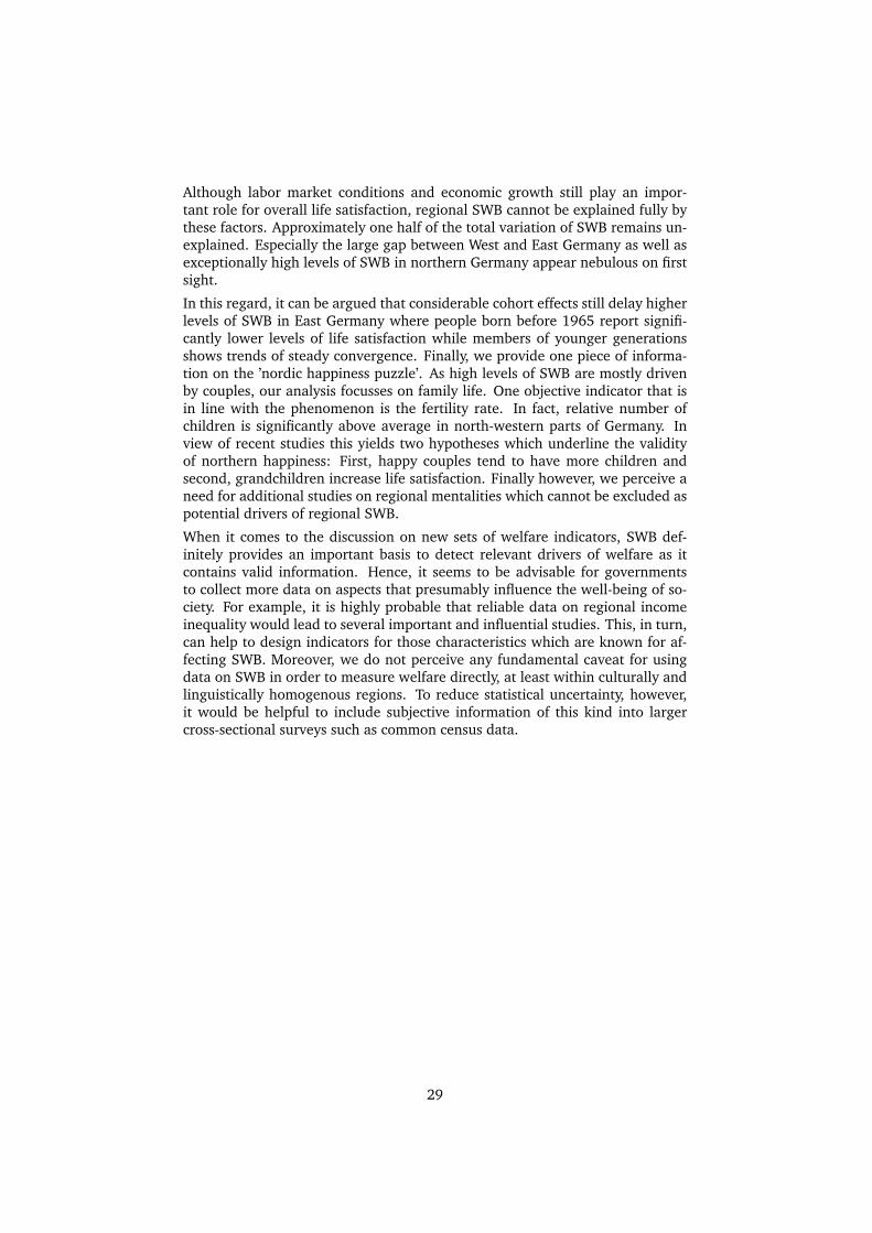
In this analyses three levels of regional subdivisions are used. For large-scalecomparisons or regressions on representative subsamples Germany is dividedinto four large regions (north, west, east and south).3 To avoid any confusionwe will refer to the former political division of Germany as East and West Ger-

3To get a detailed picture of the regional setting see Figure 8 in the appendix. The map illustratesboth the large-scale and the detailed subdivision into 19 regions.

6

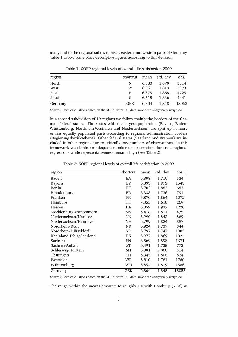
many and to the regional subdivisions as eastern and western parts of Germany.Table 1 shows some basic descriptive figures according to this devision.

Table 1: SOEP regional levels of overall life satisfaction 2009

region shortcut mean std. dev. obs.

North N 6.880 1.870 3014West W 6.861 1.813 5873East E 6.875 1.868 4725South S 6.518 1.836 4441Germany GER 6.804 1.848 18053

Sources: Own calculations based on the SOEP. Notes: All data have been analytically weighted.

In a second subdivision of 19 regions we follow mainly the borders of the Ger-man federal states. The states with the largest population (Bayern, Baden-Württemberg, Nordrhein-Westfalen and Niedersachsen) are split up in moreor less equally populated parts according to regional administration borders(Regierungsbezirksebene). Other federal states (Saarland and Bremen) are in-cluded in other regions due to critically low numbers of observations. In thisframework we obtain an adequate number of observations for cross-regionalregressions while representativeness remains high (see Table 2).

Table 2: SOEP regional levels of overall life satisfaction in 2009

region shortcut mean std. dev. obs.

Baden BA 6.898 1.710 524Bayern BY 6.893 1.972 1543Berlin BE 6.703 1.883 683Brandenburg BR 6.338 1.736 791Franken FR 6.870 1.864 1072Hamburg HH 7.355 1.610 269Hessen HE 6.859 1.937 1220Mecklenburg-Vorpommern MV 6.418 1.811 475Niedersachsen/Nordsee NN 6.990 1.842 869Niedersachsen/Hannover NH 6.799 1.824 887Nordrhein/Köln NK 6.924 1.737 844Nordrhein/Düsseldorf ND 6.797 1.747 1005Rheinland-Pfalz/Saarland RS 6.977 1.869 1024Sachsen SN 6.569 1.898 1371Sachsen-Anhalt ST 6.491 1.738 772Schleswig-Holstein SH 6.881 2.060 514Thüringen TH 6.345 1.808 824Westfalen WE 6.810 1.761 1780Württemberg WÜ 6.854 1.819 1586Germany GER 6.804 1.848 18053

Sources: Own calculations based on the SOEP. Notes: All data have been analytically weighted.

The range within the means amounts to roughly 1.0 with Hamburg (7.36) at

7

the top and Brandenburg (6.34) at the bottom. The overall mean is 6.80. Thestandard deviations alternate around 1.8. The number of observations withina single region varies from 1780 (Westfalen) to 269 (Hamburg). The averagenumber of observations per region is 950.4

Finally, an even more detailed division of 96 regions is used which follows an of-ten used spatial planning category (Raumordnungsregion). Although this sub-sample includes a lot of noise due to low numbers of observation, it is stillhelpful for additional analyses that include more detailed regional information.

3.3 Representativeness of regional data

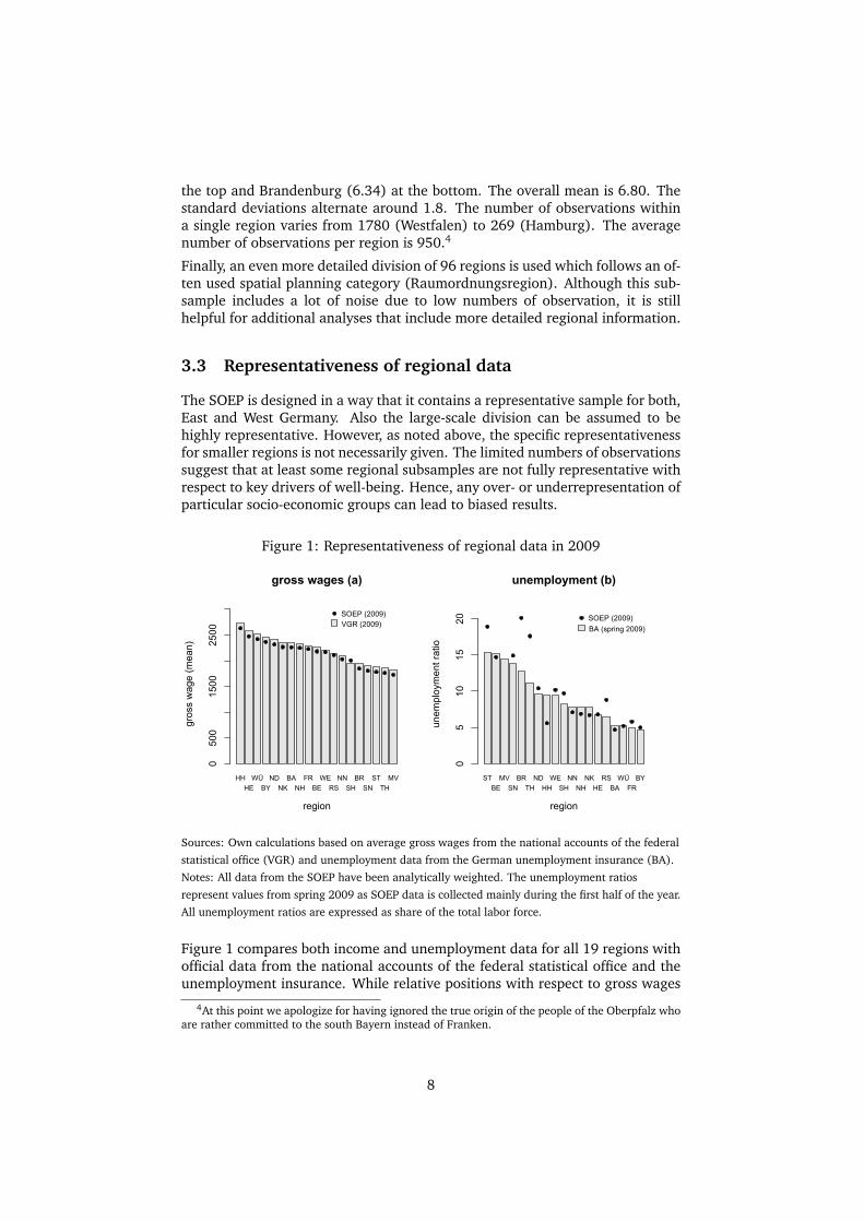
The SOEP is designed in a way that it contains a representative sample for both,East and West Germany. Also the large-scale division can be assumed to behighly representative. However, as noted above, the specific representativenessfor smaller regions is not necessarily given. The limited numbers of observationssuggest that at least some regional subsamples are not fully representative withrespect to key drivers of well-being. Hence, any over- or underrepresentation ofparticular socio-economic groups can lead to biased results.

Figure 1: Representativeness of regional data in 2009

gross wages (a)

region

gros

s w

age

(mea

n)

0500

1500

2500

HH WÜ ND BA FR WE NN BR ST MVHE BY NK NH BE RS SH SN TH

SOEP (2009)VGR (2009)

unemployment (b)

region

unem

ploy

men

t rat

io

05

1015

20

ST MV BR ND WE NN NK RS WÜ BYBE SN TH HH SH NH HE BA FR

SOEP (2009)BA (spring 2009)

Sources: Own calculations based on average gross wages from the national accounts of the federal

statistical office (VGR) and unemployment data from the German unemployment insurance (BA).

Notes: All data from the SOEP have been analytically weighted. The unemployment ratios

represent values from spring 2009 as SOEP data is collected mainly during the first half of the year.

All unemployment ratios are expressed as share of the total labor force.

Figure 1 compares both income and unemployment data for all 19 regions withofficial data from the national accounts of the federal statistical office and theunemployment insurance. While relative positions with respect to gross wages

4At this point we apologize for having ignored the true origin of the people of the Oberpfalz whoare rather committed to the south Bayern instead of Franken.

8

per employee are fully in line with the official numbers, regional unemploy-ment ratios based on the SOEP only fit roughly to institutional data. Especiallyin several states of East Germany (BR, TH and ST) the unemployment rates cal-culated on the basis of the SOEP exceed official numbers significantly. In turn,the group of unemployed seems to be underrepresented in Hamburg. This di-vergence suggests that smaller regions are biased to some extent to the one orthe other direction which has to be taken into account for the interpretation ofthe subsequent analyses.

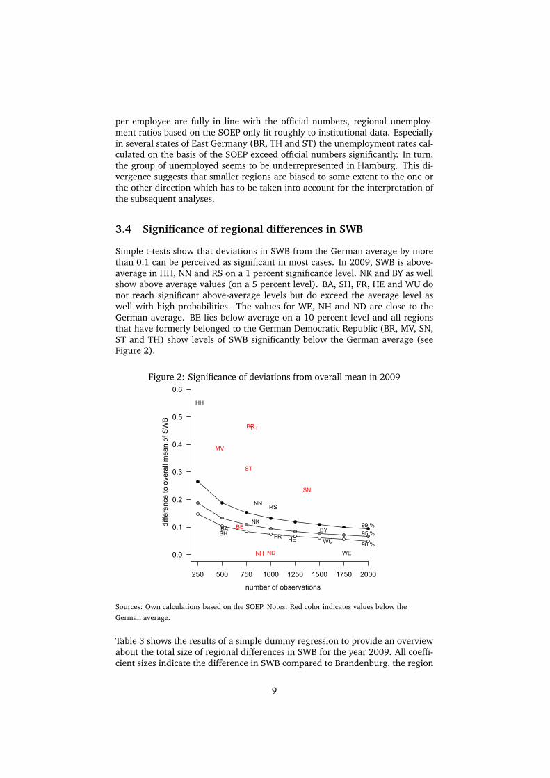
3.4 Significance of regional differences in SWB

Simple t-tests show that deviations in SWB from the German average by morethan 0.1 can be perceived as significant in most cases. In 2009, SWB is above-average in HH, NN and RS on a 1 percent significance level. NK and BY as wellshow above average values (on a 5 percent level). BA, SH, FR, HE and WU donot reach significant above-average levels but do exceed the average level aswell with high probabilities. The values for WE, NH and ND are close to theGerman average. BE lies below average on a 10 percent level and all regionsthat have formerly belonged to the German Democratic Republic (BR, MV, SN,ST and TH) show levels of SWB significantly below the German average (seeFigure 2).

Figure 2: Significance of deviations from overall mean in 2009

250 500 750 1000 1250 1500 1750 2000

0.0

0.1

0.2

0.3

0.4

0.5

0.6

number of observations

diffe

renc

e to

ove

rall

mea

n of

SW

B

BA BYBE

BR

FR

HH

HE

MV

NN

NH

NK

ND

RS

SN

ST

SH

TH

WE

WÜ

99 %95 %

90 %

Sources: Own calculations based on the SOEP. Notes: Red color indicates values below the

German average.

Table 3 shows the results of a simple dummy regression to provide an overviewabout the total size of regional differences in SWB for the year 2009. All coeffi-cient sizes indicate the difference in SWB compared to Brandenburg, the region

9

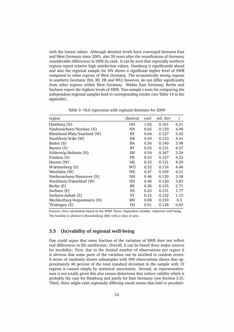
with the lowest values. Although absolute levels have converged between Eastand West Germany since 2005, also 20 years after the reunification of Germanyconsiderable differences in SWB do exist. It can be seen that especially northernregions report relative high satisfaction values. Hamburg is significantly aheadand also the regional sample for NN shows a significant higher level of SWBcompared to other regions of West Germany. The economically strong regionsin southern Germany (BA, BY, FR and WU) however, do not differ significantlyfrom other regions within West Germany. Within East Germany, Berlin andSachsen report the highest levels of SWB. Two-sample t-tests for comparing theindependent regional samples lead to corresponding results (see Table 14 in theappendix).

Table 3: OLS regression with regional dummies for 2009

region shortcut coef. std. dev. t

Hamburg (N) HH 1.02 0.161 6.31Niedersachsen/Nordsee (N) NN 0.65 0.130 4.98Rheinland-Pfalz/Saarland (W) RS 0.64 0.127 5.02Nordrhein/Köln (W) NK 0.59 0.133 4.41Baden (S) BA 0.56 0.140 3.98Bayern (S) BY 0.55 0.121 4.57Schleswig-Holstein (N) SH 0.54 0.167 3.24Franken (S) FR 0.53 0.127 4.22Hessen (W) HE 0.52 0.121 4.29Württemberg (S) WÜ 0.52 0.116 4.46Westfalen (W) WE 0.47 0.109 4.31Niedersachsen/Hannover (N) NH 0.46 0.129 3.58Nordrhein/Düsseldorf (W) ND 0.46 0.120 3.83Berlin (E) BE 0.36 0.135 2.71Sachsen (E) SN 0.23 0.131 1.77Sachsen-Anhalt (E) ST 0.15 0.132 1.15Mecklenburg-Vorpommern (N) MV 0.08 0.159 0.5Thüringen (E) TH 0.01 0.128 0.05

Sources: Own calculations based on the SOEP. Notes: Dependent variable: subjective well-being.

The baseline is allotted to Brandenburg (BR) with a value of zero.

3.5 (In)validity of regional well-being

One could argue that some fraction of the variation of SWB does not reflectreal differences in life satisfaction. Overall, it can be found three major sourcesfor invalidity: First, due to the limited number of observations per region itis obvious that some parts of the variation can be ascribed to random errors.A series of randomly drawn subsamples with 900 observations shows that ap-proximately 40 percent of the total standard deviation in the sample with 19regions is caused simply by statistical uncertainty. Second, as representative-ness is not totally given this also causes distortions that reduce validity which isprobably the case for Hamburg and partly for East Germany (see Section 3.3).Third, there might exist regionally differing social norms that lead to peculiari-

10

ties within respond behavior which do not reflect real levels of life satisfaction.Imagine, for example, that it is more common to complain about somethingopenly for people in region A than for those in region B. On the other hand,it might be culturally anchored to show modesty in region B, while communi-cation is more direct in region A. Such differences in mentality can potentiallyinfluence survey data and are difficult to detect.5

4 Macroeconomic fundamentals

4.1 Correlations

Employment and income have been detected and described as positive driversof well-being in many cases both on the individual (see, e.g., Winkelmann andWinkelmann [1995], Gerlach and Stephan [1996]) as well as on the aggregatelevel (see, e.g., DiTella et al. [2001], DiTella et al. [2003], and Stewart [2005]).The evidence endorses the fact that indicators such as GDP or unemploymentrate are the most frequently and prominently reported ones in many countries.This leads to two relevant questions: First, by how much can regional differ-ences within Germany be explained by different levels of GDP and unemploy-ment? Second, how important are both welfare indicators in relation to eachother? These questions are discussed in the following paragraphs.

Table 4: Correlation coefficients for 19 German regions from 2000 to 2009

GDP per capita economic growth unemployment

SWB .51*** -.14 -.81***GDP per capita 1 -.18* -.57***economic growth 1 .09

Sources: Own calculations based on the SOEP, Statistisches Bundesamt and Bundesagentur für

Arbeit. Notes: *** significant at 0.1 percent level; ** at 1 percent level; * at 5 percent level.

The descriptive statistics shown in Section 3 generally support the theory thataggregated levels of SWB can be explained largely by objective macroeconomicvariables such as unemployment rates or mean income.6 Unsurprisingly, SWBis negatively correlated with the degree of unemployment and positively corre-lated with the economic performance of each region. During the period from2000 to 2009, for the sample of 19 German regions, the correlation coefficientof GDP and SWB has been on average .51. In contrast, the correlation betweenregional SWB and unemployment (measured as ratio of unemployed persons

5Theoretically, one could also argue that language is understood not in the same way even withinone country due to regionally differing idioms. This would imply that the meaning of "life satisfac-tion" varies somewhat across regions. Although we do not provide any evidence, we think that thisis not of great importance as the notion "life satisfaction" (Lebenszufriedenheit) has presumably thesame meaning throughout Germany.

6We do not focus on inflation as inflation rates have been moderate in Germany since the mid-1990s. Furthermore, regional differences have been quite small due to common monetary policyand highly integrated markets for consumer goods.

11

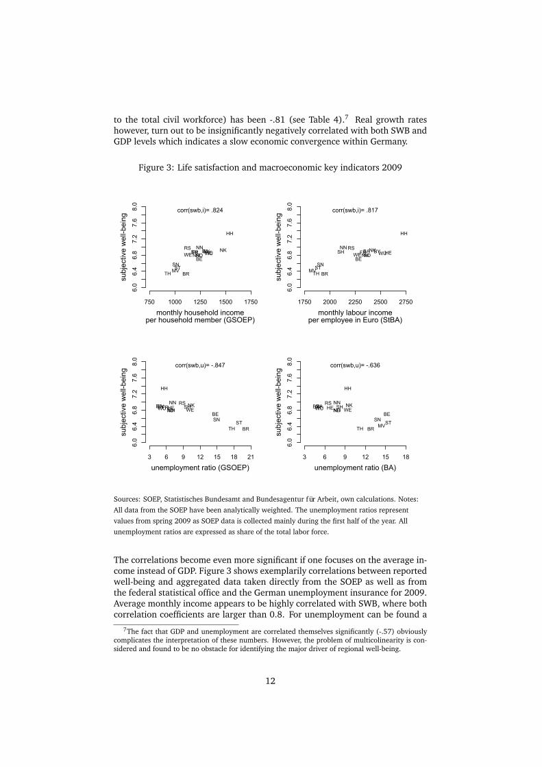
to the total civil workforce) has been -.81 (see Table 4).7 Real growth rateshowever, turn out to be insignificantly negatively correlated with both SWB andGDP levels which indicates a slow economic convergence within Germany.

Figure 3: Life satisfaction and macroeconomic key indicators 2009

750 1000 1250 1500 1750

6.0

6.4

6.8

7.2

7.6

8.0

monthly household incomeper household member (GSOEP)

subj

ectiv

e w

ell-b

eing

corr(swb,i)= .824

BABYBE

BR

FR

HH

HE

MV

NNNH

NKND

RS

SNST

SH

TH

WE WÜ

1750 2000 2250 2500 2750

6.0

6.4

6.8

7.2

7.6

8.0

monthly labour incomeper employee in Euro (StBA)

subj

ectiv

e w

ell-b

eing

corr(swb,i)= .817

BA BYBE

BR

FR

HH

HE

MV

NNNH

NKND

RS

SNST

SH

TH

WE WÜ

3 6 9 12 15 18 21

6.0

6.4

6.8

7.2

7.6

8.0

unemployment ratio (GSOEP)

subj

ectiv

e w

ell-b

eing

corr(swb,u)= -.847

BABYBE

BR

FR

HH

HE

MV

NNNH

NKND

RS

SN ST

SH

TH

WEWÜ

3 6 9 12 15 18

6.0

6.4

6.8

7.2

7.6

8.0

unemployment ratio (BA)

subj

ectiv

e w

ell-b

eing

corr(swb,u)= -.636

BABYBE

BR

FR

HH

HE

MV

NNNH

NKND

RS

SN ST

SH

TH

WEWÜ

Sources: SOEP, Statistisches Bundesamt and Bundesagentur für Arbeit, own calculations. Notes:

All data from the SOEP have been analytically weighted. The unemployment ratios represent

values from spring 2009 as SOEP data is collected mainly during the first half of the year. All

unemployment ratios are expressed as share of the total labor force.

The correlations become even more significant if one focuses on the average in-come instead of GDP. Figure 3 shows exemplarily correlations between reportedwell-being and aggregated data taken directly from the SOEP as well as fromthe federal statistical office and the German unemployment insurance for 2009.Average monthly income appears to be highly correlated with SWB, where bothcorrelation coefficients are larger than 0.8. For unemployment can be found a

7The fact that GDP and unemployment are correlated themselves significantly (-.57) obviouslycomplicates the interpretation of these numbers. However, the problem of multicolinearity is con-sidered and found to be no obstacle for identifying the major driver of regional well-being.

12

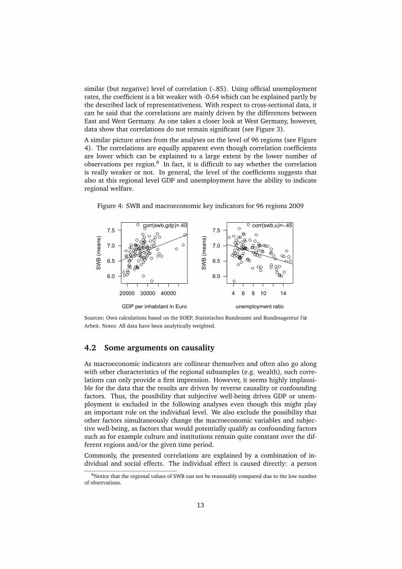
similar (but negative) level of correlation (-.85). Using official unemploymentrates, the coefficient is a bit weaker with -0.64 which can be explained partly bythe described lack of representativeness. With respect to cross-sectional data, itcan be said that the correlations are mainly driven by the differences betweenEast and West Germany. As one takes a closer look at West Germany, however,data show that correlations do not remain significant (see Figure 3).

A similar picture arises from the analyses on the level of 96 regions (see Figure4). The correlations are equally apparent even though correlation coefficientsare lower which can be explained to a large extent by the lower number ofobservations per region.8 In fact, it is difficult to say whether the correlationis really weaker or not. In general, the level of the coefficients suggests thatalso at this regional level GDP and unemployment have the ability to indicateregional welfare.

Figure 4: SWB and macroeconomic key indicators for 96 regions 2009

20000 30000 40000

6.0

6.5

7.0

7.5

GDP per inhabitant in Euro

SW

B (m

eans

)

corr(swb,gdp)=.40

4 6 8 10 14

6.0

6.5

7.0

7.5

unemployment ratio

SW

B (m

eans

)

corr(swb,u)=-.45

Sources: Own calculations based on the SOEP, Statistisches Bundesamt and Bundesagentur für

Arbeit. Notes: All data have been analytically weighted.

4.2 Some arguments on causality

As macroeconomic indicators are collinear themselves and often also go alongwith other characteristics of the regional subsamples (e.g. wealth), such corre-lations can only provide a first impression. However, it seems highly implausi-ble for the data that the results are driven by reverse causality or confoundingfactors. Thus, the possibility that subjective well-being drives GDP or unem-ployment is excluded in the following analyses even though this might playan important role on the individual level. We also exclude the possibility thatother factors simultaneously change the macroeconomic variables and subjec-tive well-being, as factors that would potentially qualify as confounding factorssuch as for example culture and institutions remain quite constant over the dif-ferent regions and/or the given time period.

Commonly, the presented correlations are explained by a combination of in-dividual and social effects. The individual effect is caused directly: a person

8Notice that the regional values of SWB can not be reasonably compared due to the low numberof observations.

13

looses her job, another receives a higher salary, etc. Social effects, however, aremultilayer. They appear first of all at the social environment of the respectiveperson, as unemployment or changes in household income also affect familymembers. Second, macroeconomic conditions cannot just be described as thesum of microeconomic happenings. They also might influence the mood of anentire society. If unemployment rises, this also might induce the fear of manyemployees to become unemployed (see, e.g., Clark et al. [2009] and Luechingeret al. [2010]) and higher contribution payments. Correspondingly, an increasein production not just leads to higher household incomes but probably alsoswells tax revenues and contributes to brighter expectations. Finally, there isno need for mentioning the well known impact of economic growth on the un-employment rate itself.9 When it comes to GDP, the relationship is even morecomplex. Although higher levels of GDP per head commonly go along withhigher incomes and more consumption, aggregated numbers on income tendto be like a black box. The examples have already been described by many re-searchers: Just think about expenditures for national defense or intelligence – itis hard to grasp the direct link that should cause any increase in subjective well-being. Furthermore, GDP obviously compromises consumption expendituresand investments alike. Fluctuations of investment or export activities (whichmostly drive business cycles) are not supposed to raise life satisfaction immedi-ately. The effects of economic growth on average SWB can also be reduced iffor example growth boosts particularly earnings at the top of the income distri-bution where people realize comparably low levels of marginal utility (Layardet al. [2008]). Focussing on positional concerns or crowding out of social inter-actions can lead to arguments where SWB can be lowered by economic growth(see, e.g., Pugno [2009] or Kolmos and Salamon [2008]). Finally, any regionalredistribution of public recourses – which is done intensively within Germany –additionally reduces the potential impact of changes in GDP. Hence, there areseveral arguments that lead to the assumption that the effects of output perhead are less significant than those of the labor market situation.

4.3 Macroeconomic estimations

The empirical strategy follows mainly the approach of Di Tella et al. (2001).In order to tackle both dimensions of causality, macro- and microeconomic re-gression models are used and finally combined by including macroeconomicvariables to microeconomic fixed effects estimations. While all microeconomicdata have its source in the SOEP, all macroeconomic data have been drawn fromthe federal statistical offices and the German unemployment insurance.

To receive elementary information about the overall effects of macroeconomicindicators on regional SWB, we started by conducting pure macroeconomic re-gressions where the dependent variable equals the weighted mean values ofreported life satisfaction SBWit of each region i in the year t:

SWBit = βXit + εi + λt + µit (1)

9Note that Okun’s law has changed significantly in Germany during the last decade. Due to labormarket reforms and the demographic changes ahead, Germany has been able to sustain employmenteven with average growth rates of less than one percent.

14

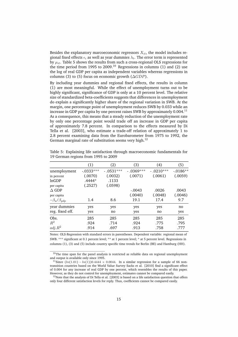
Besides the explanatory marcoeconomic regressors Xit, the model includes re-gional fixed effects εi as well as year dummies λt. The error term is representedby µit. Table 5 shows the results from such a cross-regional OLS regressions forthe time period from 1995 to 2009.10 Regressions in columns (1) and (2) usethe log of real GDP per capita as independent variables whereas regressions incolumns (3) to (5) focus on economic growth (∆GDP ).

By including year dummies and regional fixed effects, the results in column(1) are most meaningful. While the effect of unemployment turns out to behighly significant, significance of GDP is only at a 10 percent level. The relativesize of standardized beta-coefficients suggests that differences in unemploymentdo explain a significantly higher share of the regional variation in SWB. At themargin, one percentage point of unemployment reduces SWB by 0.033 while anincrease in GDP per capita by one percent raises SWB by approximately 0.004.11

As a consequence, this means that a steady reduction of the unemployment rateby only one percentage point would trade off an increase in GDP per capitaof approximately 7.8 percent. In comparison to the effects measured by DiTella et al. [2003], who estimate a trade-off relation of approximately 1 to2.8 percent examining data from the Eurobarometer from 1975 to 1992, theGerman marginal rate of substitution seems very high.12

Table 5: Explaining life satisfaction through macroeconomic fundamentals for19 German regions from 1995 to 2009

(1) (2) (3) (4) (5)

unemployment -.0333*** - .0531*** - .0369*** - .0210*** -.0186**in percent (.0070) (.0032) (.0071) (.0061) (.0059)lnGDP .4444* .1133per capita (.2527) (.0598)∆ GDP -.0043 .0026 .0043per capita (.0040) (.0048) (.0046)−βu/βgdp 1.4 8.6 19.1 17.4 9.7

year dummies yes yes yes yes noreg. fixed eff. yes no yes no yes

Obs. 285 285 285 285 285R2 .924 .714 .924 .775 .795adj.R2 .914 .697 .913 .758 .777

Notes: OLS-Regression with standard errors in parentheses. Dependent variable: regional mean of

SWB. *** significant at 0.1 percent level; ** at 1 percent level; * at 5 percent level. Regressions in

columns (1), (3) and (5) include country specific time trends for Berlin (BE) and Hamburg (HH).

10The time span for the panel analysis is restricted as reliable data on regional unemploymentand output is available only since 1995.

11Since (ln(1.01) − ln(1))0.4444 ≃ 0.0044. In a similar regression for a sample of 66 non-transition countries based on the World Value Survey Sacks et al. [2010] find a significant effectof 0.004 for any increase of real GDP by one percent, which resembles the results of this paper.However, as they do not control for unemployment, estimates cannot be compared easily.

12Note that the analysis of Di Tella et al. [2003] is based on a life satisfaction question that offersonly four different satisfaction levels for reply. Thus, coefficients cannot be compared easily.

15

However, several arguments can be brought up to explain the moderate rele-vance of GDP. First, the panel analyses is based on data from a time periodin which Germany has been significantly richer and more saturated than thecountries of the European sample during the 1970s and 1980s. Second, as onefocuses on the effects within one country, one has to take the regional redis-tribution scheme into account which e.g. transferred considerable shares ofGDP from West to East Germany during the last two decades. Third, economicgrowth has not proportionally contributed to wage increases (especially forblue-collar jobs) during the considered time span (see, e.g., Fuchs-Schündelnet al. [2010]). Thus, the estimated trade-off relation is not implausible on firstsight. The finding that unemployment probably plays a dominant role com-pared to growth can be underlined by the recent increase in SWB within EastGermany. Since 2005, the unemployment rate in East Germany has droppedrapidly from 18.7 to 13.0 percent in 2009 while reported life satisfaction hasincreased significantly from 6.3 to 6.5. In contrast, the evolution of SWB afterthe renunification has not reflected the rapid growth rates of real incomes.

The regression shown in column (2) of Table 5 excludes regional fixed effectsand provides a picture that is even more explicit. While the negative effect ofunemployment is becoming stronger, the impact of GDP is still significant onthe 10 percent level but has only one forth in size compared to column (1).Although multicollinearity weakens the significance, this strongly suggests thatthe existing regional differences in SWB can be explained much better by unem-ployment than by data on aggregated income respectively GDP. The regressionresults in columns (3) to (5) basically point into the same direction. In each ofthe regressions unemployment is highly significant whereas no significant effectof real economic growth can be found.13

Table 6: Fixed effects OLS regression for regional life satisfaction from 2001and 2009

(1) (2) (3) (4)

unemployment -.0437** -.0447*** -.0412*** - .0412***in percent (.0136) (0058) (.0072) (.0063)GDP .0082 .0100*per capita (0263) (.0041)lnGDP - .1027 .3332**per capita (.5411) (.1231)

year dummies yes yes yes yesreg. fixed eff. yes no yes no

Obs. 192 192 192 192R2 .828 .447 .828 .447

Notes: OLS-Regression with robust standard errors (in parentheses). Dependent variable: regional

mean of SWB. *** significant at 0.1 percent level; ** at 1 percent level; * at 5 percent level.

13As high growth rates do not instantly change the level of wages and salaries, we also run severalregressions with lagged growth variables which, however, do not change the results substantially.

16

Before one gives a broader interpretation of these results, it is advisable torecheck the findings by conducting regression analyses for the sample of 96regions as well. Table 6 shows the regression results for a panel with only twowaves, one in 2001 and the other one in 2009. This limited number of pointsin time is sufficient due to the high number of observations in each wave andallows us to avoid the problem of detecting effects of growth on SWB that aretime-lagged. The year 2001 has been chosen as a starting point because of adrastic increase in the number of observations in the SOEP data since 2000 andthe availability of regional unemployment data. All aggregated data have beentaken again from the federal statistical office and from the unemployment in-surance. Regressions in columns (1) and (2) use nominal GDP per capita levels(where GDP has been multiplied by a factor of 1000) as explanatory variablewhereas regressions in columns (3) and (4) use log values.14

The results are similar to the ones above even though the data contains addi-tional noise due to the low numbers of observation per region. The negativeeffect of the unemployment rate is highly significant. Also the size of the effectof unemployment is robust at a level slightly above 0.04 which is close to theprevious results. The GDP on the other hand does not enter the estimation in asignificant way, at least if regional fixed effects are included. If regional effectsare excluded, significance of both welfare indicators is increasing as one wouldexpect. However, as the point estimates of GDP and lnGDP are far from robust,there is no sense in deriving any trade-off relation from these estimations.

To sum up, the macroeconomic estimates provide evidence for the assumptionthat the total effect of one percentage point change of unemployment lies be-tween -0.3 and -0.5 depending on the regional division and whether regionalfixed effects are included or not. If one follows the estimation of regression(1) in Table 5, this would mean that a regional difference in unemployment of6 percentage points (the difference between West and East Germany in 2009)leads to a gap in SWB of approximately 0.2 on the 0-10 scale. This impliesthat approximately one half of the difference in SWB between East and WestGermany can be attributed to different levels of unemployment. Assuming aconvergence just in terms of GDP would result in a reduction of the "satisfac-tion gap" by approximately 25 percent. However, these estimates should just beclassified as a first rough approximation as other explanatory collinear variables(e.g. wealth) are not included to the model. The fact that SWB – if one looks atsmaller regions – does not reflect differences in economic growth from a periodof eight years is stunning.

4.4 Microeconomic estimations

In order to separate the effects on the individual from those on the aggregatedlevel and to control for multicolinearity we continue with several fixed effectregressions, aiming at individual life satisfaction. The OLS regression equationon a pure microeconomic level is given by

14Note that regional price levels in general change uniformly do to highly integrated markets.Hence, relative changes in nominal values of GDP also reflect relative changes in real values. How-ever, when it comes to real estate markets and rents, regional price dynamics exist to some extent.

17

SWBjit = βXjit + αi + εj + λt + µit, (2)

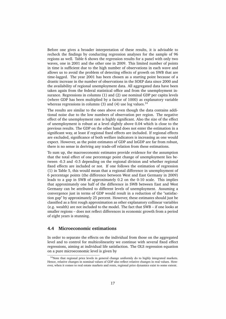
where SWBjit is the well-being level reported by individual i in country j inyear t, αi is the individual fixed effect of individual i, εj is a regional fixedeffect and λt is a year effect. As there is no need for the availability of macroe-conomic data, the time span of the analyzed panel is extended by three morewaves (1992 to 1994). The set of personal characteristics Xjit has been cho-sen according to general literature findings. The regression results are shownin Table 7 and confirm standard findings where unemployment causes a signif-icant drop in SWB and personal labor income enhances SWB with decreasingmarginal returns. If one controls for income variables, unemployment reducesSWB of a person by approximately 0.4 on the 0-10 scale (see column (3)).Without controlling for income, the size of the effect is rather -0.6 (see col-umn (2)). As those estimates are fairly robust, this already suggests that theindividual losses in life satisfaction do not account for the major part of theaggregated effects estimated in Section 4.3. This can be shown by a simple cal-culation: If the unemployment rate increases by one percent and the labor forcerepresents 70 percent of the adult population, this implies that the effects onthe individual level lower the overall mean of life satisfaction by only 0.0042(= 0.01∗0.7∗0.6) which is less than 15 percent of the macroeconomic effect (seein comparison Table 5). Income on the other hand raises SWB by approximately0.003 if real net income increases by one percent. Hence, if GDP growth is re-flected in growth in income, an increase of real GDP per capita by 10 percentshould cause a durable aggregated effect of approximately 0.03 which accountsfor two thirds of the macroeconomic effect measured above. This is plausible asGDP growth also contributes to public sector growth. However, as our macroe-conomic estimation is not very precise, it is not reasonable to note this relationas a robust finding. In addition, several authors argue that on an aggregatedlevel positional concerns potentially disperse large parts of the individual effects(see Section 2). Although one can not draw any conclusion on this question,we are highly confident in concluding that the indirect effects of unemploymentare of higher importance than the ones that lies within GDP growth. Moreover,the finding of Winkelmann and Winkelmann [1995], who argue that the indi-vidual costs of becoming unemployed sum up to high financial amounts, can berecorded.

Further interesting results are: (i) Divorced persons are happier than singlepersons who have never been married. (ii) Disposable income of householdmembers is at least as important for subjective well-being as personal income.(iii) The subjective health status plays a dominant role among explanatory vari-ables. (iv) Life satisfaction is found to be U-shaped with respect to age. (v)On average, marriage causes higher effects than cohabitation. (vi) Owning realestate is connected to higher levels of SWB.

18

Table 7: Fixed effects OLS regression for individual life satisfaction from 1992to 2009

Independent Variable (1) (2) (3) (4)

age -.0730*** -.0278*** -.0728*** -.0406***(.0038) (.0022) (.0037) (.0022)

age2 .0475*** .0047* .0539*** .0097***(.0042) (.0020) (.0041) (.0020)

SHSa "very good" .7286*** .7421*** .7355*** .7356***(.0135) (.0111) (.0132) (.0113)

SHS "good" .4095*** .3990*** .4094*** .3961***(.0082) (.0067) (.0081) (.0068)

SHS "not that good" -.5125*** -.5622*** -.5200*** -.5552***(.0126) (.0087) (.0124) (.0089)

SHS "bad" -1.4316*** -1.642*** -1.4528*** -1.6235***(.0305) (.0163) (.0299) (.0166)

married .4796*** .4012*** .4423*** .4572***(.0181) (0139) (.0176) (.0142)

with partner .3329*** .3045*** .3306*** .3072***(.0135) (0.108) (.0133) (.0110)

divorced .2171*** .1673*** .2058*** .1922***(.0240) (.0207) (.0236) (.0209)

unemployed -.3879*** -.6038*** -.3771*** -.5597***(.0344) (.0110) (.0339) (.0112)

lnYp .1116*** .1601***personal net income (.0094) (.0087)lnYh .2193*** .2973***hh net income per member (.0123) (.0089)house/flat owner .0938*** .0808*** .0949*** .0768***

(.0121) (.0100) (.0119) (.0102)R-sq (within) .0794 .0985 .0782 .1015R-sq (between) .1404 .1579 .1403 .1549R-sq (overall) .1336 .1433 .1344 .1383rho .5626 .5536 .5613 .5627Number of individuals 30320 44222 31227 42938Avg obs per ind. 5.9 7.3 6.0 7.3

Notes: OLS-Regression with individual fixed effects, individual characteristics as well as aggregate

information. Number of observations: 188069. Standard errors in parentheses. Dependent

variable: regional mean of SWB. *** significant at 0.1 percent level; ** at 1 percent level; * at 5

percent level. Regional fixed effects and year dummies have been included. aSHS: subjective

health status.

19

4.5 Combining both datasets

After having shortly introduced the results of basic microeconomic regressions,we return to the aggregated level. The combined regression equation is givenby

SWBjit = αi + β1ln(GDP )j + β2Uj +N

∑k=3

βkXkit + εj + +λt + µit (3)

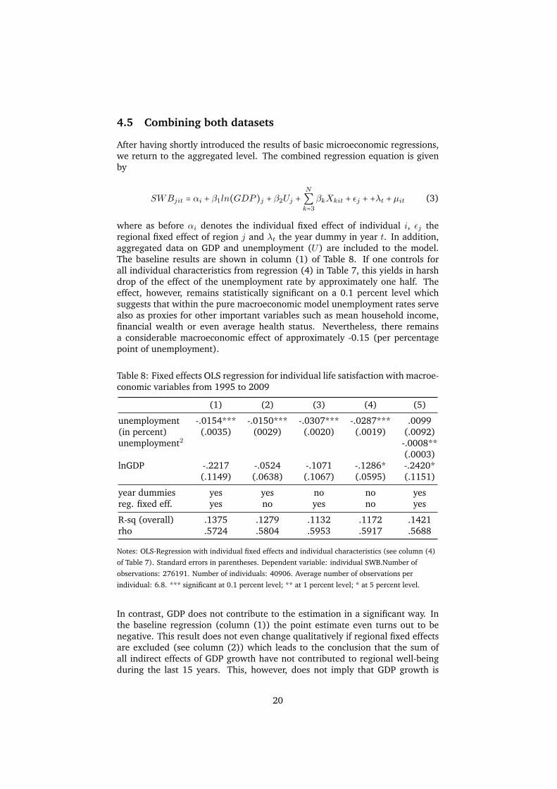
where as before αi denotes the individual fixed effect of individual i, εj theregional fixed effect of region j and λt the year dummy in year t. In addition,aggregated data on GDP and unemployment (U) are included to the model.The baseline results are shown in column (1) of Table 8. If one controls forall individual characteristics from regression (4) in Table 7, this yields in harshdrop of the effect of the unemployment rate by approximately one half. Theeffect, however, remains statistically significant on a 0.1 percent level whichsuggests that within the pure macroeconomic model unemployment rates servealso as proxies for other important variables such as mean household income,financial wealth or even average health status. Nevertheless, there remainsa considerable macroeconomic effect of approximately -0.15 (per percentagepoint of unemployment).

Table 8: Fixed effects OLS regression for individual life satisfaction with macroe-conomic variables from 1995 to 2009

(1) (2) (3) (4) (5)

unemployment -.0154*** -.0150*** -.0307*** -.0287*** .0099(in percent) (.0035) (0029) (.0020) (.0019) (.0092)unemployment2 -.0008**

(.0003)lnGDP -.2217 -.0524 -.1071 -.1286* -.2420*

(.1149) (.0638) (.1067) (.0595) (.1151)

year dummies yes yes no no yesreg. fixed eff. yes no yes no yes

R-sq (overall) .1375 .1279 .1132 .1172 .1421rho .5724 .5804 .5953 .5917 .5688

Notes: OLS-Regression with individual fixed effects and individual characteristics (see column (4)

of Table 7). Standard errors in parentheses. Dependent variable: individual SWB.Number of

observations: 276191. Number of individuals: 40906. Average number of observations per

individual: 6.8. *** significant at 0.1 percent level; ** at 1 percent level; * at 5 percent level.

In contrast, GDP does not contribute to the estimation in a significant way. Inthe baseline regression (column (1)) the point estimate even turns out to benegative. This result does not even change qualitatively if regional fixed effectsare excluded (see column (2)) which leads to the conclusion that the sum ofall indirect effects of GDP growth have not contributed to regional well-beingduring the last 15 years. This, however, does not imply that GDP growth is

20

obsolete for the country as a whole, although the negative coefficient for logGDP even turns out to be significant as soon as time and regional dummiesare excluded (see column (4)). That this is a false conclusion can be easilyseen if one considers the regional distribution of public net investments withinGermany since the reunification. In fact, the stock of public infrastructure hasincreased in per capita terms especially in those regions where it has been onthe lowest levels. This hypothesis is one out of many and cannot be discussedhere in detail.

What can be discussed instead is how much of the regional variance can beexplained by unemployment and differences in income. Figure 5 shows the un-explained regional effects of both the microeconomic as well as the combinedregression model. In comparison to the total variation of SWB in 2009, which isillustrated by the dark bars, it can be seen that significant parts but not the ma-jority of regional differences can be attributed to macroeconomic fundamentals.For most regions within East Germany, however, considerable negative effectsstill remain. In contrast, Hamburg and the very northwest of Germany still showsurprisingly high values of SWB. Nevertheless, approximately 40 percent of thegap in life satisfaction between East and West Germany can be attributed tofundamental macroeconomic conditions.

Figure 5: Unexplained regional deviation 2009

HH RS BA SH HE WE ND SN MV BR

region

unex

plai

ned

regi

onal

dev

iatio

n of

SW

B

-0.6

-0.4

-0.2

0.0

0.2

0.4

0.6

NN NK BY FR WU NH BE ST TH

total deviation of SWBmicroeconomic estimationestimation with combined data

Source: Own calculations based on the regression results in Tables 7 and 8.

21

4.6 The marginal disutility of unemployment

To complete the analyses of Sections 4.1 to 4.5, it can be argued that the impactof macroeconomic fundamentals is not equal in size within each region partlydue to nonlinearity of effects. With respect to GDP and household income thishas been considered by using log values as marginal utility diminishes both onthe individual and on the aggregate level (Sacks et al. [2010]). However, whenit comes to unemployment, things are less obvious. In fact, there are severalarguments that counter the simple idea of constant marginal effects of unem-ployment as well. However, as one has to take into account always both groups,the employed and the unemployed, this is more tricky. In theory, the employedare harmed by unemployment at least in two ways: First, high unemployment isconnected to lower job security. In other words, the higher the unemployment isthe more afraid of layoffs employees become. Second, employees who witnesslayoffs might suffer as well due to feelings of guilt and a worsening of socialclimate at work. Some more linkages are discussed by Clark et al. (2009).What we want to emphasize is that these arguments only apply if unemploy-ment exceeds some basic level. If, in contrast, unemployment is only a problemof persons with deficits in basic qualifications, it is not plausible that this causesany fear among the employed. The same is true if unemployment mainly oc-curs due to persons who enter the labor market after education or change jobsvoluntarily. As a consequence, the negative effects of unemployment on theemployed would only be considerable if unemployment is caused by structurallabor market distortions such as high labor costs or business cycles which leadto unemployment rates that exceed a basic level. This can be a potential expla-nation for an increase in marginal disutility of unemployment on the aggregatelevel which is indicated by regression (5) in Table 8.

With respect to the unemployed Clark [2003] provides evidence from the BritishHousehold Survey and argues that higher unemployment numbers help the un-employed to cope with their "violation" of the social norm not to live from publicfunds. Hence, some authors have concluded that a rise in unemployment easesthe disutility of the unemployed which as a consequence would contribute to adecrease in marginal disutility of unemployment. For Germany, however, em-pirical evidence is not in line with any conclusion that ascribes a dominant roleto this effect. Regionally separated fixed effects regressions show significantlystronger effects of unemployment for eastern parts of Germany where unem-ployment rates have been nearly twice as high during the last two decades (seeTable 9). On the other hand, the effect has been significant but rather low forsouthern Germany where unemployment has remained on a comparably lowlevel during the same time period. Similar findings have been also made byChadi [2011] who emphasizes the effect of lower job prospects in presence ofhigh unemployment rates. Overall, we do not want to conclude on possiblecauses at this point, but there is evidence suggesting increasing marginal disu-tility for both groups, the employed as well as the unemployed. Hence, it canbe assumed that differing levels of unemployment contribute even more to theregional variation of SWB, in particular with respect to the difference betweenEast and West Germany.

22

Table 9: Fixed effects OLS regression for individual life satisfaction by regionfrom1992 to 2009

Independent Variable (north) (west) (south) (east)

age -.1136*** -.1156*** -.1287*** -.0451***(.0030) (.0189) (.0205) (.0106)

age2 .0535*** .0479*** .0469*** .0463***(.0136) (.0097) (.01060) (.0120)

SHSa "very good" .7585*** .7071*** .7662*** .6908***(.0369) (.0259) (.0272) (.0321)

SHS "good" .4078*** .4024*** .4258*** .3984***(.0231) (.0155) (.0178) (.0187)

SHS "not that good" -.4910*** -.5106*** -.5911*** -.4739***(.0396) (.0267) (.0309) (.0327)

SHS "bad" -1.4902*** -1.482*** -1.496*** -1.3141***(.0396) (.0869) (.0909) (.0977)

married .5253*** .4552*** .4825*** .3709***(.0626) (0446) (.0469) (.0556)

with partner .4034*** .3331*** .3227*** .3006***(.0433) (.0313) (.0326) (.0370)

divorced .1446*** .2567*** .2142** .2177**(.0806) (.0577) (.0653) (.0682)

unemployed -.3973*** -.4803*** -.2093 -.5248***(.1150) (.0866) (.1094) (.0700)

net labor income .0092*** .0128*** .0113*** .0274***in 100 Euro (.0024) (.0013) (.0014) (.0024)net labor income2 -.0012*** -.0015*** -.0014*** -.0058***

(.0003) (.0002) (.0002) (.0010)house/flat owner .0504*** .1008*** .07847* .0317*

(.0149) (.0262) (.0282) (.0317)R-sq (within) .0794 .0865 .0898 .0669R-sq (between) .0346 .0302 .0329 .0019R-sq (overall) .0447 .0388 .0487 .0090rho .6668 .6631 .6950 .6842number of obs. 29447 62240 51570 44812

Notes: OLS-Regression with individual fixed effects, year dummies and regional fixed effects.

Standard errors in parentheses. Dependent variable: regional mean of SWB. *** significant at 0.1

percent level; ** at 1 percent level; * at 5 percent level. Regional fixed effects and year dummies

have been included. aSHS: subjective health status.

23

5 Other explanatory factors

Obviously, the regional levels of well-being are not just a result from macro-economic conditions. It can rather be assumed that numerous factors exert aninfluence on the overall SWB within one country or region while not all of themare easy to detect or durable over time. The following paragraphs discuss onlytwo aspects that help understand the remaining pattern of unexplained regionalSWB.

5.1 Communistic heritage

Thus far, the comparably low levels of SWB in East Germany have been ex-plained to a large extent by lower incomes and higher unemployment rates.However, a considerable part of the satisfaction gap between East and WestGermany remains unexplained. To solve this puzzle it is helpful to focus on sin-gle generations. Table 10 reports SWB for different age groups in West and EastGermany for the year 2009. The values indicate strong cohort effects. Note thatthose aged 30 and older in 1990 report far lower satisfaction levels than theirwestern counterparts. In comparison to the younger generation the differencein SWB is nearly twice as large for individuals born before 1960. In 2009, thedifference in SWB between the generation aged 30 and younger of East andWest Germany has been 2.5 times smaller compared to the difference betweenthose aged 50 and older (see Table 10).

Table 10: SWB in East and West Germany for different age groups in 2009

age group in yrs. 20-29 30-39 40-49 50-59 60-69 70-79

West Germany 7.07 7.11 6.66 6.58 6.98 6.94East Germany 6.89 6.81 6.39 6.07 6.50 6.46Absolute difference 0.18 0.30 0.27 0.51 0.48 0.48

Source: SOEP. Notes: Weighted. Number of observations: 18053.

To complement this cross-sectional data, Figure 6 shows by how much the meanSWB of the respectively younger generation (35 years and below) exceeds thesatisfaction level of the older generation (older than 35). While the relativehappiness of the younger generation has only slightly increased in West Ger-many, it has risen dramatically for East Germany especially between 1995 and2005: Directly after reunification there has been only a difference of approxi-mately 0.2. In 2009, when the young generation consisted of individuals bornafter 1974, the difference in SWB between the generations accounted for morethan 0.5.These data suggest that those generations who have not just grown up withinthe German Democratic Republic, but also spend a considerable share of theirworking life under the communistic regime are significantly worse off. Whetherthis finding is connected mainly to difficulties of adjusting to the mechanisms ofa free and competitive labor market, to the anger of having spend irretrievableyears under limited freedom or to durable disappointments about the failure ofsocialistic policy – to name just a few possible root causes – cannot be discussed

24

Figure 6: Absolute difference in SWB between the generations

1992 1994 1996 1998 2000 2002 2004 2006 2008

0.0

0.1

0.2

0.3

0.4

0.5

0.6

year

diffe

renc

e in

SW

B b

etw

een

gene

ratio

ns

West GermanyEast Germany

Source: SOEP. Notes: Weighted. At any time the young generation consists of those younger than

35. The old generation is defined respectively as the group aged 35 and older.

here. Nevertheless, it is safe to say that the low levels of reported life satisfactionin East Germany are still linked to the cultural imprints of many who have spentparts of their lives in the former DDR. Thus, it can be assumed that one wouldperceive a partial convergence of SWB in the future even if macroeconomicconditions do not continue to converge.

5.2 A note on the nordic happiness puzzle

Besides the huge differences between East and West Germany, there are alsocomparably high values of reported life satisfaction in northern Germany whichremain mostly unexplained (see Figure 5). Again, it is helpful to analyze thedata separately. Table 11 shows mean values of SWB of different age groupsfor each part of Germany. Note that the relatively high levels of life satisfac-tion within the North of Germany are mainly driven by the elderly. For thegroup aged 60 and older, northern Germany reports considerably higher num-bers (7.08) than their economically stronger counterparts in southern Germany(6.90), whereas the generation between 35 and 60 reports lower levels of SWBthan this generation in the West and the South of Germany.

These high values of SWB can neither be explained by differing levels of unem-ployment nor by differing income structures as both variables would indicatean inverse relation. One indication for the origin of this phenomenon can befound within family life. Table 12 summarizes the satisfaction responses for allpersons aged 60 or older by marital status. While the share of people without

25

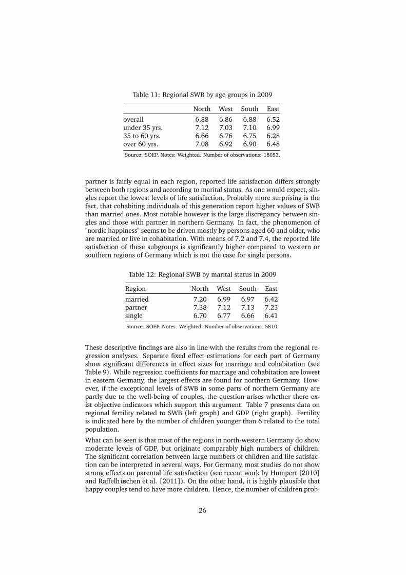
Table 11: Regional SWB by age groups in 2009

North West South East

overall 6.88 6.86 6.88 6.52under 35 yrs. 7.12 7.03 7.10 6.9935 to 60 yrs. 6.66 6.76 6.75 6.28over 60 yrs. 7.08 6.92 6.90 6.48

Source: SOEP. Notes: Weighted. Number of observations: 18053.

partner is fairly equal in each region, reported life satisfaction differs stronglybetween both regions and according to marital status. As one would expect, sin-gles report the lowest levels of life satisfaction. Probably more surprising is thefact, that cohabiting individuals of this generation report higher values of SWBthan married ones. Most notable however is the large discrepancy between sin-gles and those with partner in northern Germany. In fact, the phenomenon of"nordic happiness" seems to be driven mostly by persons aged 60 and older, whoare married or live in cohabitation. With means of 7.2 and 7.4, the reported lifesatisfaction of these subgroups is significantly higher compared to western orsouthern regions of Germany which is not the case for single persons.

Table 12: Regional SWB by marital status in 2009

Region North West South East

married 7.20 6.99 6.97 6.42partner 7.38 7.12 7.13 7.23single 6.70 6.77 6.66 6.41

Source: SOEP. Notes: Weighted. Number of observations: 5810.

These descriptive findings are also in line with the results from the regional re-gression analyses. Separate fixed effect estimations for each part of Germanyshow significant differences in effect sizes for marriage and cohabitation (seeTable 9). While regression coefficients for marriage and cohabitation are lowestin eastern Germany, the largest effects are found for northern Germany. How-ever, if the exceptional levels of SWB in some parts of northern Germany arepartly due to the well-being of couples, the question arises whether there ex-ist objective indicators which support this argument. Table 7 presents data onregional fertility related to SWB (left graph) and GDP (right graph). Fertilityis indicated here by the number of children younger than 6 related to the totalpopulation.

What can be seen is that most of the regions in north-western Germany do showmoderate levels of GDP, but originate comparably high numbers of children.The significant correlation between large numbers of children and life satisfac-tion can be interpreted in several ways. For Germany, most studies do not showstrong effects on parental life satisfaction (see recent work by Humpert [2010]and Raffelhüschen et al. [2011]). On the other hand, it is highly plausible thathappy couples tend to have more children. Hence, the number of children prob-

26

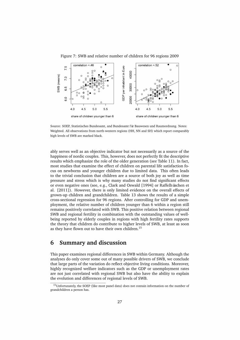
Figure 7: SWB and relative number of children for 96 regions 2009

Source: SOEP, Statistisches Bundesamt, and Bundesamt für Bauwesen und Raumordnung. Notes:

Weighted. All observations from north-western regions (HH, NN and SH) which report comparably

high levels of SWB are marked black.

ably serves well as an objective indicator but not necessarily as a source of thehappiness of nordic couples. This, however, does not perfectly fit the descriptiveresults which emphasize the role of the older generation (see Table 11). In fact,most studies that examine the effect of children on parental life satisfaction fo-cus on newborns and younger children due to limited data. This often leadsto the trivial conclusion that children are a source of both joy as well as timepressure and stress which is why many studies do not find significant effectsor even negative ones (see, e.g., Clark and Oswald [1994] or Raffelhüschen etal. [2011]). However, there is only limited evidence on the overall effects ofgrown-up children and grandchildren. Table 13 shows the results of a simplecross-sectional regression for 96 regions. After controlling for GDP and unem-ployment, the relative number of children younger than 6 within a region stillremains positively correlated with SWB. This positive relation between regionalSWB and regional fertility in combination with the outstanding values of well-being reported by elderly couples in regions with high fertility rates supportsthe theory that children do contribute to higher levels of SWB, at least as soonas they have flown out to have their own children.15

6 Summary and discussion

This paper examines regional differences in SWB within Germany. Although theanalyses do only cover some out of many possible drivers of SWB, we concludethat large parts of the variation do reflect objective living conditions. Moreover,highly recognized welfare indicators such as the GDP or unemployment ratesare not just correlated with regional SWB but also have the ability to explainthe evolution and differences of regional levels of SWB.

15Unfortunately, the SOEP (like most panel data) does not contain information on the number ofgrandchildren a person has.

27

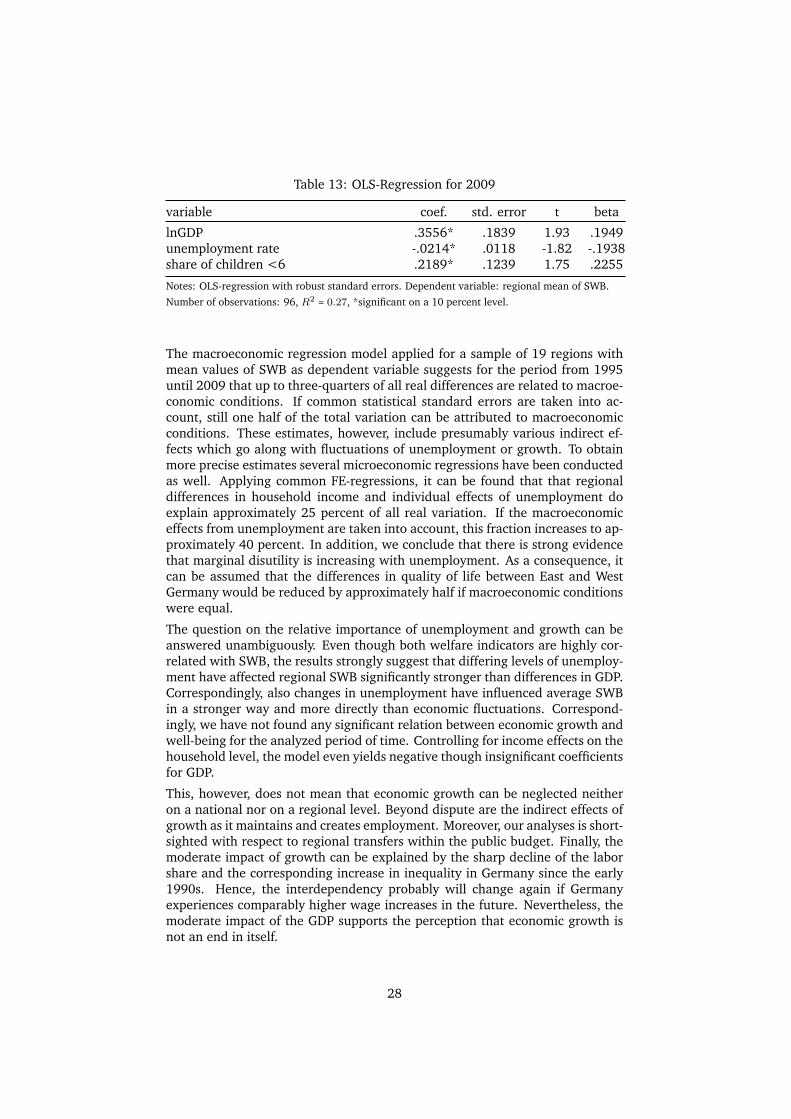
Table 13: OLS-Regression for 2009

variable coef. std. error t beta

lnGDP .3556* .1839 1.93 .1949unemployment rate -.0214* .0118 -1.82 -.1938share of children <6 .2189* .1239 1.75 .2255

Notes: OLS-regression with robust standard errors. Dependent variable: regional mean of SWB.

Number of observations: 96, R2= 0.27, *significant on a 10 percent level.

The macroeconomic regression model applied for a sample of 19 regions withmean values of SWB as dependent variable suggests for the period from 1995until 2009 that up to three-quarters of all real differences are related to macroe-conomic conditions. If common statistical standard errors are taken into ac-count, still one half of the total variation can be attributed to macroeconomicconditions. These estimates, however, include presumably various indirect ef-fects which go along with fluctuations of unemployment or growth. To obtainmore precise estimates several microeconomic regressions have been conductedas well. Applying common FE-regressions, it can be found that that regionaldifferences in household income and individual effects of unemployment doexplain approximately 25 percent of all real variation. If the macroeconomiceffects from unemployment are taken into account, this fraction increases to ap-proximately 40 percent. In addition, we conclude that there is strong evidencethat marginal disutility is increasing with unemployment. As a consequence, itcan be assumed that the differences in quality of life between East and WestGermany would be reduced by approximately half if macroeconomic conditionswere equal.

The question on the relative importance of unemployment and growth can beanswered unambiguously. Even though both welfare indicators are highly cor-related with SWB, the results strongly suggest that differing levels of unemploy-ment have affected regional SWB significantly stronger than differences in GDP.Correspondingly, also changes in unemployment have influenced average SWBin a stronger way and more directly than economic fluctuations. Correspond-ingly, we have not found any significant relation between economic growth andwell-being for the analyzed period of time. Controlling for income effects on thehousehold level, the model even yields negative though insignificant coefficientsfor GDP.

This, however, does not mean that economic growth can be neglected neitheron a national nor on a regional level. Beyond dispute are the indirect effects ofgrowth as it maintains and creates employment. Moreover, our analyses is short-sighted with respect to regional transfers within the public budget. Finally, themoderate impact of growth can be explained by the sharp decline of the laborshare and the corresponding increase in inequality in Germany since the early1990s. Hence, the interdependency probably will change again if Germanyexperiences comparably higher wage increases in the future. Nevertheless, themoderate impact of the GDP supports the perception that economic growth isnot an end in itself.

28

Although labor market conditions and economic growth still play an impor-tant role for overall life satisfaction, regional SWB cannot be explained fully bythese factors. Approximately one half of the total variation of SWB remains un-explained. Especially the large gap between West and East Germany as well asexceptionally high levels of SWB in northern Germany appear nebulous on firstsight.

In this regard, it can be argued that considerable cohort effects still delay higherlevels of SWB in East Germany where people born before 1965 report signifi-cantly lower levels of life satisfaction while members of younger generationsshows trends of steady convergence. Finally, we provide one piece of informa-tion on the ’nordic happiness puzzle’. As high levels of SWB are mostly drivenby couples, our analysis focusses on family life. One objective indicator that isin line with the phenomenon is the fertility rate. In fact, relative number ofchildren is significantly above average in north-western parts of Germany. Inview of recent studies this yields two hypotheses which underline the validityof northern happiness: First, happy couples tend to have more children andsecond, grandchildren increase life satisfaction. Finally however, we perceive aneed for additional studies on regional mentalities which cannot be excluded aspotential drivers of regional SWB.

When it comes to the discussion on new sets of welfare indicators, SWB def-initely provides an important basis to detect relevant drivers of welfare as itcontains valid information. Hence, it seems to be advisable for governmentsto collect more data on aspects that presumably influence the well-being of so-ciety. For example, it is highly probable that reliable data on regional incomeinequality would lead to several important and influential studies. This, in turn,can help to design indicators for those characteristics which are known for af-fecting SWB. Moreover, we do not perceive any fundamental caveat for usingdata on SWB in order to measure welfare directly, at least within culturally andlinguistically homogenous regions. To reduce statistical uncertainty, however,it would be helpful to include subjective information of this kind into largercross-sectional surveys such as common census data.

29

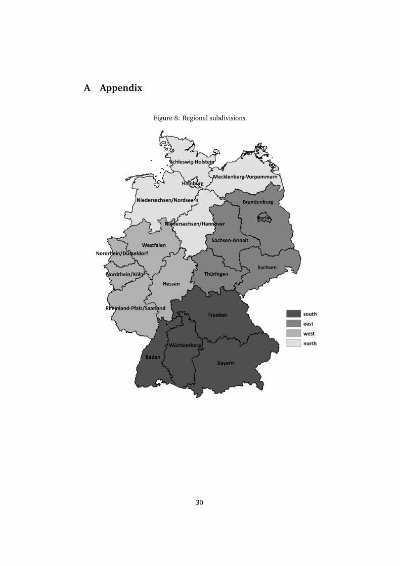
A Appendix

Figure 8: Regional subdivisions

30

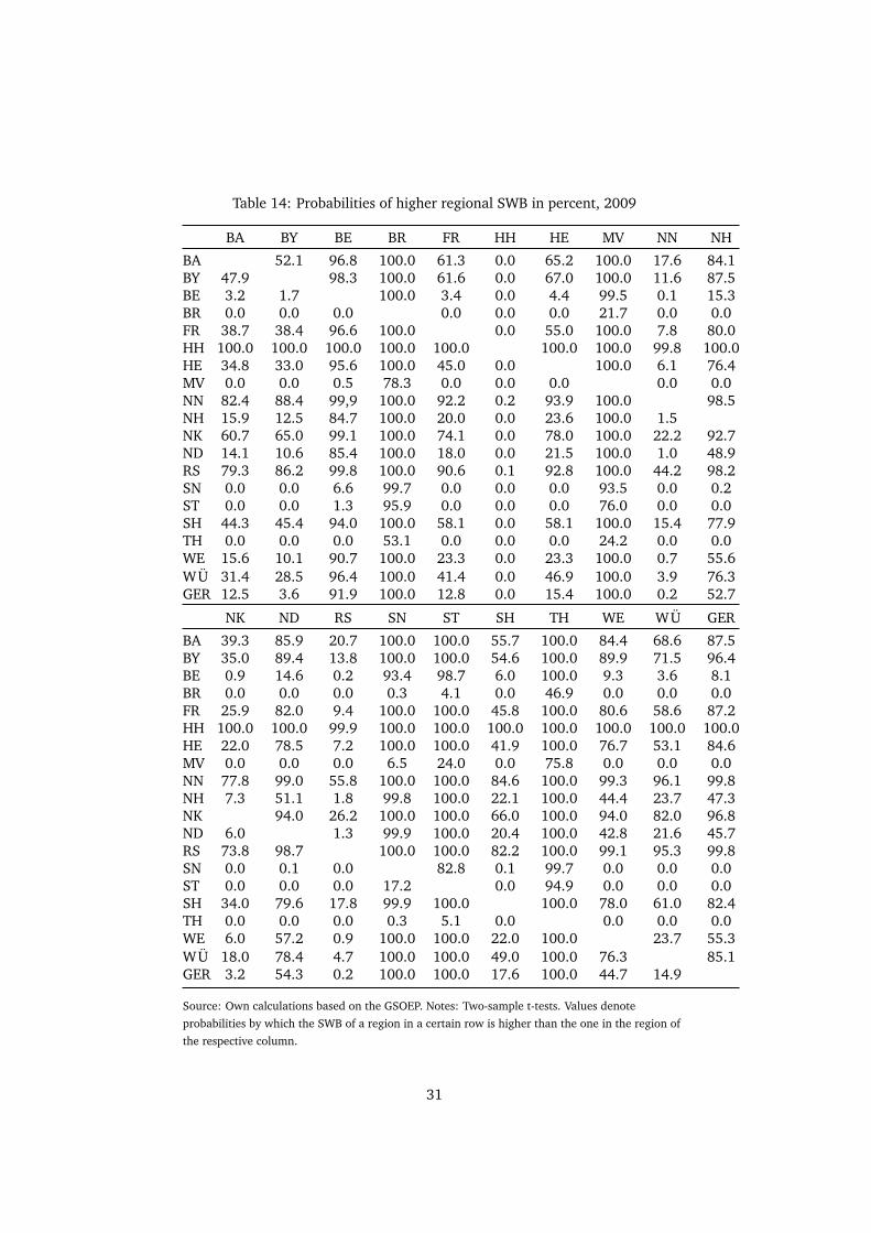
Table 14: Probabilities of higher regional SWB in percent, 2009

BA BY BE BR FR HH HE MV NN NH

BA 52.1 96.8 100.0 61.3 0.0 65.2 100.0 17.6 84.1BY 47.9 98.3 100.0 61.6 0.0 67.0 100.0 11.6 87.5BE 3.2 1.7 100.0 3.4 0.0 4.4 99.5 0.1 15.3BR 0.0 0.0 0.0 0.0 0.0 0.0 21.7 0.0 0.0FR 38.7 38.4 96.6 100.0 0.0 55.0 100.0 7.8 80.0HH 100.0 100.0 100.0 100.0 100.0 100.0 100.0 99.8 100.0HE 34.8 33.0 95.6 100.0 45.0 0.0 100.0 6.1 76.4MV 0.0 0.0 0.5 78.3 0.0 0.0 0.0 0.0 0.0NN 82.4 88.4 99,9 100.0 92.2 0.2 93.9 100.0 98.5NH 15.9 12.5 84.7 100.0 20.0 0.0 23.6 100.0 1.5NK 60.7 65.0 99.1 100.0 74.1 0.0 78.0 100.0 22.2 92.7ND 14.1 10.6 85.4 100.0 18.0 0.0 21.5 100.0 1.0 48.9RS 79.3 86.2 99.8 100.0 90.6 0.1 92.8 100.0 44.2 98.2SN 0.0 0.0 6.6 99.7 0.0 0.0 0.0 93.5 0.0 0.2ST 0.0 0.0 1.3 95.9 0.0 0.0 0.0 76.0 0.0 0.0SH 44.3 45.4 94.0 100.0 58.1 0.0 58.1 100.0 15.4 77.9TH 0.0 0.0 0.0 53.1 0.0 0.0 0.0 24.2 0.0 0.0WE 15.6 10.1 90.7 100.0 23.3 0.0 23.3 100.0 0.7 55.6WÜ 31.4 28.5 96.4 100.0 41.4 0.0 46.9 100.0 3.9 76.3GER 12.5 3.6 91.9 100.0 12.8 0.0 15.4 100.0 0.2 52.7

NK ND RS SN ST SH TH WE WÜ GER

BA 39.3 85.9 20.7 100.0 100.0 55.7 100.0 84.4 68.6 87.5BY 35.0 89.4 13.8 100.0 100.0 54.6 100.0 89.9 71.5 96.4BE 0.9 14.6 0.2 93.4 98.7 6.0 100.0 9.3 3.6 8.1BR 0.0 0.0 0.0 0.3 4.1 0.0 46.9 0.0 0.0 0.0FR 25.9 82.0 9.4 100.0 100.0 45.8 100.0 80.6 58.6 87.2HH 100.0 100.0 99.9 100.0 100.0 100.0 100.0 100.0 100.0 100.0HE 22.0 78.5 7.2 100.0 100.0 41.9 100.0 76.7 53.1 84.6MV 0.0 0.0 0.0 6.5 24.0 0.0 75.8 0.0 0.0 0.0NN 77.8 99.0 55.8 100.0 100.0 84.6 100.0 99.3 96.1 99.8NH 7.3 51.1 1.8 99.8 100.0 22.1 100.0 44.4 23.7 47.3NK 94.0 26.2 100.0 100.0 66.0 100.0 94.0 82.0 96.8ND 6.0 1.3 99.9 100.0 20.4 100.0 42.8 21.6 45.7RS 73.8 98.7 100.0 100.0 82.2 100.0 99.1 95.3 99.8SN 0.0 0.1 0.0 82.8 0.1 99.7 0.0 0.0 0.0ST 0.0 0.0 0.0 17.2 0.0 94.9 0.0 0.0 0.0SH 34.0 79.6 17.8 99.9 100.0 100.0 78.0 61.0 82.4TH 0.0 0.0 0.0 0.3 5.1 0.0 0.0 0.0 0.0WE 6.0 57.2 0.9 100.0 100.0 22.0 100.0 23.7 55.3WÜ 18.0 78.4 4.7 100.0 100.0 49.0 100.0 76.3 85.1GER 3.2 54.3 0.2 100.0 100.0 17.6 100.0 44.7 14.9

Source: Own calculations based on the GSOEP. Notes: Two-sample t-tests. Values denote

probabilities by which the SWB of a region in a certain row is higher than the one in the region of

the respective column.

31

References

Alesina, A., R. DiTella, and R. J. MacCulloch (2004). Inequality and happiness:are europeans and americans different? Journal of Public Economics 88(9-10),2009–2042.

Bergheim, S. (2008). Well-being in germany – its happy regions have much incommon. Deutsche Bank Research.

Berlemann, M. and C. Kemmesies (2004). Zur entwicklung der lebenszufrieden-heit nach der deutschen wiedervereinigung - eine empirische analyse in sach-sen, ost- und westdeutschland. ifo Dresden berichtet (6), 3–10.

Bjørnskov, C. (2006). The multiple facets of social capital. European Journal ofPolitical Economy 22(1), 22–40.

Blanchflower, D. and A. J. Oswald (2008). Hypertension and happiness acrossnations. Journal of Health Economics 27(2), 218–233.

Blanchflower, D. G. and A. J. Oswald (2004). Well-being over time in britainand the usa. Journal of Public Economics 88(7-8), 1359–1386.

Böhnke, P. and U. Kohler (2010). Handbook of European Societies. Social Trans-formations in the 21st Century, Chapter Well-being and Inequality, pp. 629–666. New York: Springer Science.

Chadi, A. (2011). Regional unemployment and norm-induced effects on lifesatisfaction. SOEPpapers on Multidisciplinary Panel Data Research (387).

Clark, A. E. (2003). Unemployment as a social norm: Psychological evidencefrom panel data. Journal of Labor Economics 21(2), 323–351.

Clark, A. E., P. Frijters, and M. A. Shields (2008). Relative income, happiness,and utility: An explanation for the easterlin paradox and other puzzles. Jour-nal of Economic Literature 46(1), 95–144.

Clark, A. E., A. Knabe, and S. Rätzel (2009). Unemployment as a social normin germany. Schmollers Jahrbuch 129(2), 251–260.

Clark, A. E. and A. J. Oswald (1994). Unhappiness and unemployment. TheEconomic Journal 104(424), 648–659.

Diener, E., M. Diener, and C. Diener (1995). Factors predicting the subjectivewell-being of nations. Journal of Personality and Social Pschology 69(5), 851–864.

Diener, E. and H.-D. Klingelmann (2000). Culture and subjective well-being,Chapter Genes, Culture, Democracy, and Happiness, pp. 165–183. MIT Press.

Diener, E. and W. Tov (2012). Handbook of Social Indicators and Quality of LifeResearch, Chapter National Accounts of Well-Being, pp. 137–157. Springer.

DiTella, R., R. J. MacCulloch, and A. J. Oswald (2001). Preferences over infla-tion and unemployment: Evidence from survey of happiness. The AmericanEconomic Review 91(1), 335–341.

32

DiTella, R., R. J. MacCulloch, and A. J. Oswald (2003). The macroeconomics ofhappiness. The Review of Economics and Statistics 85(4), 809–827.

Easterlin, R. A. (1974). Does economic growth improve the human a lot? someempirical evidence. In P. A. David and M. W. Reder (Eds.), Nations and House-holds in Economic Growth: Essays in Honor of Moses Abramowitz, pp. 89–125.Academic Press.

Easterlin, R. A. (2005). Diminishing marginal utility of income? caveat emptor.Sical Indicators Research 70(3), 243–255.

Easterlin, R. A. and A. C. Plagnol (2008). Life satisfaction and economic condi-tions in east and west germany pre- and post-unification. Journal of EconomicBehavior and Organization 68(3-4), 433–444.

Frey, B. S. and A. Stutzer (2002). Happiness and Economics. Princeton UniversityPress.

Fuchs-Schündeln, N., D. Krueger, and M. Sommer (2010). Inequality trends forgermany in the last two decades: A tale of two countries. Review of EconomicDynamics 13(1), 103–132.

Gerlach, K. and G. Stephan (1996). A paper on unhappiness and unemploymentin germany. Economic Letters 52(3), 325–330.

Helliwell, J. F. (2003). How’s life? combining individual and national variablesto explain subjective well-being. Economic Modelling 20(2), 331–360.

Humpert, S. (2010). Machen kinder doch glücklich? SOEPpapers on Multidisci-plinary Panel Data Research 301.

Kahneman, D. and A. B. Krueger (2006). Developments in the measurement ofsubjective well-being. Journal of Economic Perspectives 20(1), 3–24.

Kahneman, D., A. B. Krueger, D. Schkade, and N. Schwarz (2004). Towardnational well-being accounts. American Economic Review 94(2), 429–434.

Kolmos, J. and P. Salamon (2008). The poverty of growth with interdependentutitity functions. The Journal of Socio-Economics 37(6), 2242–2247.

Kristensen, N. and E. Johansson (2008). New evidence on cross-country differ-ences in job satisfaction using anchoring vignettes. Labour Economics 15(1),96–117.

Lane, R. E. (2000). The Loss of Happiness in Market Democracies. Yale ISPSSeries. New Haven and London: Yale University Press.

Layard, R. (2010). Measuring subjective well-being. Science 327, 534–535.

Layard, R., G. Mayraz, and S. J. Nickell (2008). The marginal utility of income.Journal of Public Economics 92(8-9), 1846–1857.

Luechinger, S. (2011). Valuing air quality using the life satisfaction approach.The Economic Journal 110(536), 482–515.

33

Luechinger, S., S. Meier, and A. Stutzer (2010). Why does unemployment hurtthe employed? evidence from the life satisfaction gap between the public andthe private sector. Journal of Human Resources 45(4), 989–1045.

Maddison, D. and K. Rehdanz (2007). Are regional differences in utility elim-inated over time? evidence from germany. SOEPpapers on MultidisciplinaryPanel Data Research (16).

Ng, Y.-K. (2003). From preference to happiness: Towards a more completewarfare economics. Social Choice and Welfare 20(2), 307–350.

Oishi, S., S. Kesebir, and E. Diener (2011). Income inequality and happiness.Psychological Science 22(9), 1095–1100.

Oswald, A. J. (1997). Happiness and economic performance. The EconomicJournal 107(445), 1815–1831.

Oswald, A. J. and S. Wu (2010). Objective confirmation of subjective measuresof human well-being: Evidence from the u.s.a. Science 327, 576–579.

Pugno, M. (2009). The easterlin paradox and the decline of social capital: Anintegrated explanation. The Journal of Socio-Economics 38(4), 590–600.

Raffelhüschen, B., S. Moog, and J. Vatter (2011). Glücksatlas Deutschland 2011,Chapter Wie zufrieden ist Deuschland?, pp. 29–138. Deutsche Post.

Rousseau, J.-B. G. (2009). Happiness and income inequality. mimeo.

Sachverständigenrat (2010). Wirtschaftsleistung, lebensqualität und nach-haltigkeit: Ein umfassendes indikatorensystem. Sachverständigenrat zurBegutachtung der gesamtwirtschaftlichen Entwicklung and Conseil d’Analyseéconomique.

Sacks, D. W., B. Stevenson, and J. Wolfers (2010). Subjective well-being, in-come, economic development and growth. NBER Working Paper (16441).

Shields, M. A. and S. W. Price (2005). Exploring the economic and social deter-minants of psychological wellbeing and perceived social support in england.Journal of the Royal Statistical Society 168(3), 513–537.

Stewart, K. (2005). Dimensions of well-being in eu regions: Do gdp and un-employment tell us all we need to know? Social Indicators Researchn 73(2),221–246.

Veenhoven, R. and J. Ehrhardt (1995). The cross-national pattern of happiness:Test of predictions implied in three theories of happiness. Social IndicatorsResearch 34(1), 33–68.

Vittersø, J., R. Biswas-Diener, and E. Diener (2005). The divergent meanings oflife satisfaction: Item response modeling of the satisfaction with life scale ingreenland and norway. Social Indicators Research 74(2), 327–348.

Wagner, G. G., J. R. Frick, and J. Schupp (2007). The german socio-economicpanel study (soep) - scope, evolution and enhancements. SchmollersJahrbuch 127(1), 139–169.

34

Wierzbicka, A. (2005). Empirical universals of language as a basis for the studyof other human universals and as a tool for exploring cross-cultural differ-ences. Ethos 33(2), 256–291.

Winkelmann, R. and L. Winkelmann (1995). Happiness and unemployment: apanel data analysis for germany. Konjunkturpolitik 41(4), 293–307.

35