Smokeview (Version 6) - A Tool for Visualizing Fire ... · NIST Special Publication 1017-3. Smokeview (Version 6) A Tool for Visualizing Fire Dynamics Simulation Data Volume III:

NIST Special Publication 1017-3

Smokeview (Version 6)A Tool for Visualizing

Fire Dynamics Simulation DataVolume III: Verification Guide

Glenn P. Forney

karenw

Typewritten Text

http://dx.doi.org/10.6028/NIST.SP.1017-3

karenw

Typewritten Text

karenw

Typewritten Text

NIST Special Publication 1017-3

Smokeview (Version 6)A Tool for Visualizing

Fire Dynamics Simulation DataVolume III: Verification Guide

Glenn P. ForneyFire Research Division

Engineering Laboratory

August 2013Smokeview Version 6

SVN Repository Revision : 16665

UN

ITE

DSTATES OF AM

ER

ICA

DE

PARTMENT OF COMMERC

E

U.S. Department of CommercePenny Pritzker, Secretary

National Institute of Standards and TechnologyPatrick D. Gallagher, Under Secretary of Commerce for Standards and Technology and Director

karenw

Typewritten Text


Certain commercial entities, equipment, or materials may be identified in this document in order todescribe an experimental procedure or concept adequately. Such identification is not intended to imply

recommendation or endorsement by the National Institute of Standards and Technology, nor is it intendedto imply that the entities, materials, or equipment are necessarily the best available for the purpose.

National Institute of Standards and Technology Special Publication 1017-3Natl. Inst. Stand. Technol. Spec. Publ. 1017-3, 101 pages (August 2013)

CODEN: NSPUE2

karenw

Typewritten Text


Preface

This guide is part of a three volume set of companion documents describing how to use Smokeview in Vol-ume I, the Smokeview User’s Guide [1], describing technical details of how the visualizations are performedin Volume II, the Smokeview Technical Reference Guide [2], and presents example cases verifying the var-ious visualization capabilities of Smokeview in Volume III, the Smokeview Verification Guide [3]. Detailson the use and technical background of the Fire Dynamics Simulator is contained in the FDS User’s [4] andTechnical reference guide [5] respectively. This guide is Volume III the Smokeview Verification guide.

Smokeview is a software tool designed to visualize numerical calculations generated by fire modelssuch as the Fire Dynamics Simulator (FDS), a computational fluid dynamics (CFD) model of fire-drivenfluid flow or the Consolidated Fire and Smokeview Transport (CFAST) model, a zone fire model. ThisGuide is Volume 3 of the Smokeview Reference Guides. This guide presents a series of images derivedfrom FDS and Smokeview. The intent is to verify that the algorithms used by Smokeview for visualizingdata are implemented correctly. These images are generated automatically through the use of scripts byfirst running FDS on a series of input cases and then running Smokeview, again using a set of scripts. Thecorrectness of Smokeview may then be verified more easily as FDS and Smokeview are updated since thereference figures in this document may be generated simply and automatically.

Smokeview and associated documentation for Windows, Linux and Mac OS X may be downloadedfrom http://fire.nist.gov/fds .

i

http://fire.nist.gov/fds

ii

About the Author

Glenn Forney is a computer scientist at the Engineering Laboratory of NIST. He received a bachelor ofscience degree in mathematics from Salisbury State College and a master of science and a doctorate inmathematics from Clemson University. He joined NIST in 1986 (then the National Bureau of Standards)and has since worked on developing tools that provide a better understanding of fire phenomena, mostnotably Smokeview, a software tool for visualizing Fire Dynamics Simulator data.

iii

iv

Disclaimer

The US Department of Commerce makes no warranty, expressed or implied, to users of Smokeview, andaccepts no responsibility for its use. Users of Smokeview assume sole responsibility under Federal law fordetermining the appropriateness of its use in any particular application; for any conclusions drawn from theresults of its use; and for any actions taken or not taken as a result of analysis performed using this tools.

Smokeview and the companion program FDS is intended for use only by those competent in the fieldsof fluid dynamics, thermodynamics, combustion, and heat transfer, and is intended only to supplement theinformed judgment of the qualified user. These software packages may or may not have predictive capabilitywhen applied to a specific set of factual circumstances. Lack of accurate predictions could lead to erroneousconclusions with regard to fire safety. All results should be evaluated by an informed user.

Throughout this document, the mention of computer hardware or commercial software does not con-stitute endorsement by NIST, nor does it indicate that the products are necessarily those best suited for theintended purpose.

v

vi

Contents

Preface i

About the Author iii

Disclaimer v

1 Overview 1

2 Data File Tests 32.1 Surface contours (Boundary Files) . . . . . . . . . . . . . . . . . . . . . . . . . . . . . . . 52.2 Iso-surfaces . . . . . . . . . . . . . . . . . . . . . . . . . . . . . . . . . . . . . . . . . . . 7

2.2.1 Sensitivity Analysis . . . . . . . . . . . . . . . . . . . . . . . . . . . . . . . . . . . . 102.3 Particles . . . . . . . . . . . . . . . . . . . . . . . . . . . . . . . . . . . . . . . . . . . . . 122.4 Slices . . . . . . . . . . . . . . . . . . . . . . . . . . . . . . . . . . . . . . . . . . . . . . 142.5 3D Smoke . . . . . . . . . . . . . . . . . . . . . . . . . . . . . . . . . . . . . . . . . . . . 222.6 Plot3D . . . . . . . . . . . . . . . . . . . . . . . . . . . . . . . . . . . . . . . . . . . . . . 23

3 Smoke Visualization Tests 293.1 Recording Smoke Levels . . . . . . . . . . . . . . . . . . . . . . . . . . . . . . . . . . . . 293.2 Verifying Smoke Levels . . . . . . . . . . . . . . . . . . . . . . . . . . . . . . . . . . . . . 30

4 WUI Test Cases 354.1 FDS Cases . . . . . . . . . . . . . . . . . . . . . . . . . . . . . . . . . . . . . . . . . . . . 354.2 WFDS Cases . . . . . . . . . . . . . . . . . . . . . . . . . . . . . . . . . . . . . . . . . . 42

5 Other Tests 475.1 Obstacles . . . . . . . . . . . . . . . . . . . . . . . . . . . . . . . . . . . . . . . . . . . . 475.2 Devices . . . . . . . . . . . . . . . . . . . . . . . . . . . . . . . . . . . . . . . . . . . . . 495.3 Vents . . . . . . . . . . . . . . . . . . . . . . . . . . . . . . . . . . . . . . . . . . . . . . . 505.4 Conversion to Color . . . . . . . . . . . . . . . . . . . . . . . . . . . . . . . . . . . . . . . 535.5 GPU Test . . . . . . . . . . . . . . . . . . . . . . . . . . . . . . . . . . . . . . . . . . . . 56

Bibliography 59

References 60

Appendices 60

A Input Files 61A.1 colorbar . . . . . . . . . . . . . . . . . . . . . . . . . . . . . . . . . . . . . . . . . . . . . 61

vii

A.2 colorconv . . . . . . . . . . . . . . . . . . . . . . . . . . . . . . . . . . . . . . . . . . . . 61A.3 fed_test . . . . . . . . . . . . . . . . . . . . . . . . . . . . . . . . . . . . . . . . . . . . . 62A.4 plume5c . . . . . . . . . . . . . . . . . . . . . . . . . . . . . . . . . . . . . . . . . . . . . 62A.5 sillytexture . . . . . . . . . . . . . . . . . . . . . . . . . . . . . . . . . . . . . . . . . . . . 64A.6 smoke_sensor . . . . . . . . . . . . . . . . . . . . . . . . . . . . . . . . . . . . . . . . . . 65A.7 smoke_test . . . . . . . . . . . . . . . . . . . . . . . . . . . . . . . . . . . . . . . . . . . . 65A.8 smoke_test2 . . . . . . . . . . . . . . . . . . . . . . . . . . . . . . . . . . . . . . . . . . . 66A.9 transparency . . . . . . . . . . . . . . . . . . . . . . . . . . . . . . . . . . . . . . . . . . . 67A.10 tree_test2 . . . . . . . . . . . . . . . . . . . . . . . . . . . . . . . . . . . . . . . . . . . . 67A.11 vcirctest . . . . . . . . . . . . . . . . . . . . . . . . . . . . . . . . . . . . . . . . . . . . . 68A.12 vcirctest2 . . . . . . . . . . . . . . . . . . . . . . . . . . . . . . . . . . . . . . . . . . . . 69

B Smokeview Scripts 71B.1 colorbar . . . . . . . . . . . . . . . . . . . . . . . . . . . . . . . . . . . . . . . . . . . . . 71B.2 colorconv . . . . . . . . . . . . . . . . . . . . . . . . . . . . . . . . . . . . . . . . . . . . 71B.3 fed_test . . . . . . . . . . . . . . . . . . . . . . . . . . . . . . . . . . . . . . . . . . . . . 73B.4 plume5c . . . . . . . . . . . . . . . . . . . . . . . . . . . . . . . . . . . . . . . . . . . . . 73B.5 sillytexture . . . . . . . . . . . . . . . . . . . . . . . . . . . . . . . . . . . . . . . . . . . . 84B.6 smoke_sensor . . . . . . . . . . . . . . . . . . . . . . . . . . . . . . . . . . . . . . . . . . 84B.7 smoke_test . . . . . . . . . . . . . . . . . . . . . . . . . . . . . . . . . . . . . . . . . . . . 84B.8 smoke_test2 . . . . . . . . . . . . . . . . . . . . . . . . . . . . . . . . . . . . . . . . . . . 85B.9 sprinkler_many . . . . . . . . . . . . . . . . . . . . . . . . . . . . . . . . . . . . . . . . . 85B.10 transparency . . . . . . . . . . . . . . . . . . . . . . . . . . . . . . . . . . . . . . . . . . . 86B.11 tree_test2 . . . . . . . . . . . . . . . . . . . . . . . . . . . . . . . . . . . . . . . . . . . . 86B.12 vcirctest . . . . . . . . . . . . . . . . . . . . . . . . . . . . . . . . . . . . . . . . . . . . . 86B.13 vcirctest2 . . . . . . . . . . . . . . . . . . . . . . . . . . . . . . . . . . . . . . . . . . . . 87

viii

List of Figures

2.1 The temperatures in the plume5c.fds case are initialized to 600 ◦C within the region outlinedin blue. . . . . . . . . . . . . . . . . . . . . . . . . . . . . . . . . . . . . . . . . . . . . . 4

2.2 Boundary file test of shaded and chopped contours . . . . . . . . . . . . . . . . . . . . . . . 62.3 A test showing an isosurface enclosing a region initialized to 600 ◦C . . . . . . . . . . . . . 82.4 A test showing isosurfaces colored orange and blue using the ISOCOLORS .ini keyword. . . 92.5 A portion of an iso-surface defined by f (x,y,z) = Tm (for some arbitrary function f ) crossing

a line segment at the point (xm,y,z). . . . . . . . . . . . . . . . . . . . . . . . . . . . . . . 102.6 Diagram setting up an inverse linear interpolation calculation . . . . . . . . . . . . . . . . . 112.7 A test showing particles and particle streaks . . . . . . . . . . . . . . . . . . . . . . . . . . 132.8 A test showing shaded and chopped contours of node centered slice file data . . . . . . . . . 152.9 A test showing shaded and chopped contours of cell centered slice file data . . . . . . . . . . 162.10 A test to demonstrate that cell centered slice file data is transferred from FDS to Smokeview

properly. . . . . . . . . . . . . . . . . . . . . . . . . . . . . . . . . . . . . . . . . . . . . . 172.11 A test showing vector slice file data . . . . . . . . . . . . . . . . . . . . . . . . . . . . . . . 182.12 A test showing cell centered FED slice file data . . . . . . . . . . . . . . . . . . . . . . . . 192.13 A test showing arbitrarily oriented slice file planes generated from 3D slice files . . . . . . . 202.14 A test showing slice contours generated by differencing two cases with Smokediff . . . . . . 212.15 A test showing 3D smoke drawn at 1 s, 10 s and 30 s . . . . . . . . . . . . . . . . . . . . . 222.16 A test showing PLOT3D stepped and continuous temperature contours. . . . . . . . . . . . 232.17 A test showing PLOT3D stepped contours at four positions along the y axis. . . . . . . . . . 242.18 A test showing PLOT3D narrow band contours at four positions along the y axis. . . . . . . 252.19 A test showing PLOT3D vectors shaded by temperature at four positions along the y axis. . . 262.20 A test showing PLOT3D iso-surfaces for 50 ◦C, 230 ◦C, 410 ◦C and 590 ◦C. . . . . . . . . . 27

3.1 A test verifying that the Smokeview smoke_sensor object is working properly . . . . . . . . 303.2 Shade of grey resolution test. . . . . . . . . . . . . . . . . . . . . . . . . . . . . . . . . . . 313.3 Side view of numerical smoke test compartment. . . . . . . . . . . . . . . . . . . . . . . . 323.4 A test verifying the smoke opacity calculation . . . . . . . . . . . . . . . . . . . . . . . . . 33

4.1 A test showing level set slices drawn along a sloped terrain . . . . . . . . . . . . . . . . . . 364.2 A test showing a fire line slice drawn along a sloped and textured terrain . . . . . . . . . . . 374.3 A test showing a fire line slice drawn along a sloped and textured terrain at 1800 s simulated

time. . . . . . . . . . . . . . . . . . . . . . . . . . . . . . . . . . . . . . . . . . . . . . . . 384.4 A test showing level temperature slices drawn along a sloped terrain . . . . . . . . . . . . . 394.5 A test showing wind vectors drawn using data obtained from a wind sensor. . . . . . . . . . 414.6 A test showing trees drawn as Smokeview objects. . . . . . . . . . . . . . . . . . . . . . . . 424.7 A test showing four states of smokeview tree objects. . . . . . . . . . . . . . . . . . . . . . 424.8 A test showing trees drawn as particles. . . . . . . . . . . . . . . . . . . . . . . . . . . . . 434.9 A test showing trees drawn as isosurfaces. . . . . . . . . . . . . . . . . . . . . . . . . . . . 44

ix

4.10 A test showing particles drawn as canopy objects. . . . . . . . . . . . . . . . . . . . . . . . 45

5.1 A test showing 3 drawing modes for representing blockages: solid, outline and hidden . . . . 485.2 A test showing that transparent objects are drawn properly . . . . . . . . . . . . . . . . . . 485.3 A test showing that devices are drawn properly . . . . . . . . . . . . . . . . . . . . . . . . 495.4 A test showing 3 modes for drawing vents: show all vents, hide open vents and hide all vents 505.5 A test showing circular vents drawn as specified in the input file and as implemented within

FDS. The circular vents are applied to a blockage. . . . . . . . . . . . . . . . . . . . . . . . 515.6 A test showing circular vents drawn as specified in the input file and as implemented within

FDS. The circular vents are applied to the external boundary. . . . . . . . . . . . . . . . . . 525.7 A test showing that data is converted to color properly . . . . . . . . . . . . . . . . . . . . . 545.8 A test showing that data is converted to color properly . . . . . . . . . . . . . . . . . . . . . 555.9 A test showing that the GPU is properly used to draw smoke . . . . . . . . . . . . . . . . . 57

x

Chapter 1

Overview

Smokeview is a scientific software tool designed to visualize numerical predictions generated by fire modelssuch as the Fire Dynamics Simulator (FDS), a computational fluid dynamics (CFD) model of fire-driven fluidflow [5, 4] or the Consolidated Fire and Smoke Transport (CFAST) model, a zone model of compartmentfire phenomena [6].

The feature set and user interface for Smokeview is complex making it difficult to adequately test all ofits features manually. A scripting capability has been added to solve this problem. Many of Smokeview’sfeatures may now be run without user intervention through the use of scripts. A script is simply a text filecontaining one or more commands. Smokeview may then read the script commands and perform the actionslisted. Some of these actions are loading data files, setting view points, setting times and most importantlyrendering images. By designing a set of scenarios and corresponding images that demonstrate Smokeview’sfeature set, one may test Smokeview running a series of scripts (one script for each test case) and examiningthe resulting images to ensure that the fire model generating the results and Smokeview are working asexpected.

This document then verifies that various Smokeview features are working as intended by presenting aseries of simulation results in the form of Smokeview images. These images are generated using the variousvisualization features of Smokeview such as tracer particles, 2D or 3D contours, or realistic smoke.

Verification in the context of Smokeview is a process to check the correctness of the visualization.Verification does not imply that the underlying data is correct, only that the data is presented or visualizedcorrectly. A separate document, the FDS Verification Guide [7], describes the verification process of FDS.One set of scripts is used to run FDS cases and a second set of scripts is used by Smokeview to generateimages. The verification process then becomes much easier to accomplish since the use of scripts (i.e.,non-manual methods) guarantees that consistent figures (same view points, same time points, same datafiles loaded, etc.) are produced as new versions of this verification document are generated using updatedversions of FDS and/or Smokeview. Another way of looking at this verification process is to consider thisdocument and the FDS Verification Guide [7] as being a live (not a static) document, easily updated asalgorithms in FDS and/or Smokeview are enhanced and improved.

Details on setting up and running FDS cases may be found in the FDS User’s Guide [4]. Details on visu-alizing FDS simulated data using Smokeview may be found in the Smokeview User’s Guide [1]. Details onsome of the technical aspects used to implement algorithms in Smokeview may be found in the SmokeviewTechnical Guide [2].

The FDS version used to run the cases illustrated in this document is

Fire Dynamics Simulator

1

Version: FDS 6, Release Candidate 4; MPI Disabled; OpenMP DisabledSVN Revision Number: 16557Compile Date: Mon, 12 Aug 2013

Consult FDS Users Guide Chapter, Running FDS, for further instructions.

Hit Enter to Escape...

The Smokeview version used to generate the verification figures in this document is

Smokeview 6.1.2 - Aug 13 2013

Version: 6.1.2Smokeview (64 bit) Revision Number: 16567Platform: WIN64 (Intel C/C++)Build Date: Aug 13 2013

FDS generated data is presumed to be correct. FDS has its own set of verification cases to test thecorrectness of the data. The purpose of the cases used here is to confirm that data is drawn or visualizedcorrectly. In particular, these cases confirm that correct files are loaded, data is scaled and drawn correctly,geometry is drawn correctly, etc. Three types of verification cases are presented. The first set are the mostimportant. Those cases verify that data is drawn correctly. The second set of cases verify that variousgeometric elements are drawn correctly and the third set verifies that the various options and underlyingfeatures are implemented and perform properly.

The FDS input files used for the verification cases are documented in Appendix A. The Smokeviewscripts used to generate the verification figures are documented in Appendix B. Note that these input filesand scripts are located in the FDS Subversion (SVN) repository. In fact, the entries in the appendices areincluded directly from the repository, and will therefore be up to date as this document is regenerated.

2

Chapter 2

Data File Tests

The tests in this chapter verify whether visualization types such as surface contours (boundary files), isosur-faces, particles, slice files, 3D smoke files and PLOT3D files are working as intended. These verificationtests all use the same FDS input file, plume5c.fds (see Appendix A.4), to generate the simulation data.The case models a simple fire plume with two blockages. The upper blockage is initialized to 600 ◦C. Thelower blockage is initialized to 20 ◦C. The gas phase is initialized to 600 ◦C within an interior region col-ored blue as illustrated in Fig. 2.1 and 20 ◦C everywhere else. This is done in order to verify that a knowntemperature is converted to the proper color (as shown in the color bar).

The verification figures are generated automatically using the Smokeview script file, plume5c.ssf(see Appendix B.4). The use of scripting allows the figures and hence this document to be updated easily aschanges are made in FDS, Smokeview or the FDS input data files. This allows the verification process to beongoing.

3

Figure 2.1: The temperatures in the plume5c.fds case are initialized to 600 ◦C within the region outlined inblue.

4

2.1 Surface contours (Boundary Files)

Figure 2.2 presents images verifying the display of surface contours or boundary file data. A series ofboundary file images are drawn at 2 s (approximately), 10 s and 30 s seconds. The temperature of the upperobstacle is initialized to 600 ◦C hence the red colors for the t = 0 s images. The first column of imagescolors data at cell nodes using temperatures averaged at surrounding cell centers. The second column ofimages colors data using data values at cell centers.

5

cell averaged data chopped data cell centered data

Figure 2.2: Boundary file test of shaded and chopped contours at 2 s, 10 s and 30 s. The upper obstacle isinitialized to 600 ◦C and should be red for the t ≈ 2 s images. For the chopped contours, the color near thechop boundary should match the color near 140 ◦C in the colorbar.

6

2.2 Iso-surfaces

An isosurface is a three-dimensional surface that defines constant values of a dependent variable. Figures2.3 and 2.4 present images verifying the display of isosurfaces. A series of temperature isosurfaces aredrawn at 0 s, 10 s and 30 s. A portion of the interior gas temperature is initialized to 600 ◦C, hence. This isthe reason that the rectangular block appears in the first row of images. The first column in Fig. 2.3 presentsthe iso-surface using points. The second column presents the iso-surface using triangulated outlines. Thethird column presents the iso-surface using a solid surface. Figure 2.4 demonstrates color customizationusing the ISOCOLORS .ini keyword.

7

point view outline view solid view

Figure 2.3: A test showing an isosurface enclosing a region initialized to 600 ◦C at 0 s, 10 s and 30 s. Theisosurface should surround this region for the t = 0 s images.

8

solid view - orange solid view - blue

Figure 2.4: A test showing isosurfaces colored orange and blue using the ISOCOLORS .ini keyword at 30 s.The two isosurfaces are colored orange and blue using the ISOCOLORS .ini keyword.

9

(x1,y,z) (x2,y,z)(xm,y,z)

T1 T2Tm

Figure 2.5: A portion of an iso-surface defined by f (x,y,z) = Tm (for some arbitrary function f ) crossing aline segment at the point (xm,y,z).

2.2.1 Sensitivity Analysis

Given that data used to generate an isosurface has uncertainty, an important question to consider is howsensitive is the isosurface location to uncertainty in the data used to define it? Figure 2.5 shows a portion ofan iso-surface, f (x,y,z) = Tm, passing through a line segment at (xm,y,z). The line segment is defined byendpoints (x1,y,z) and (x2,y,z). The key step in constructing an isosurface is solving an inverse interpolationproblem. That is, determining the location, (xm,y,z), between two grid nodes, (x1,y,z) and (x2,y,z), whereinterpolated data takes on a particular value (the isosurface level, Tm, being constructed).

Suppose, as illustrated in Fig. 2.6, that (x1,y,z), T1 and (x2,y,z), T2 represent two known data location,data value pairs and that Tm is also known satisfying T1 ≤ Tm ≤ T2. The inverse interpolation problem thenis to find the location (xm,y,z) that takes on the data value Tm. The location xm is given by

xm = (1−α)x1 +αx2 (2.1)

where

α =Tm−T1

T2−T1(2.2)

The sensitivity of xm due to a change ∆T1 in T1 and to a change ∆T2 in T2 is given by

∆xm =∂xm

∂T1∆T1 +

∂xm

∂T2∆T2 (2.3)

where∂xm

∂T1=

∂xm

∂α

∂α

∂T1(2.4)

∂xm

∂T2=

∂xm

∂α

∂α

∂T2(2.5)

10

x1 xm x2

Tm

T2

T1(xm-x1)/(x2-x1)=(Tm-T1)/(T2-T1)

Figure 2.6: Diagram setting up an inverse linear interpolation calculation. The dependent data values T1 andT2 are known at locations x1 and x2. The inverse interpolation problem is to find the location xm that hasvalue Tm. This is found noting that (xm− x1)/(x2− x1) = (Tm−T1)/(T2−T1).

and

∂xm

∂α= x2− x1 (2.6)

∂α

∂T1=

Tm−T2

(T2−T1)2 (2.7)

∂α

∂T2= − Tm−T1

(T2−T1)2 (2.8)

Equation (2.3) may be re-written using terms in equations (2.4) through (2.8) to obtain

∆xm

x2− x1=

Tm−T2

(T2−T1)2 ∆T1−Tm−T1

(T2−T1)2 ∆T2 =−((1−α)

∆T1

T2−T1+α

∆T2

T2−T1

)(2.9)

Equation (2.9) relates the relative error of xm to the relative errors of T1 and T2 in terms of the interpolationparameter α . The error ∆xm may then be bounded to obtain

|∆xm| ≤ |x2− x1|max(|∆T1|, |∆T2|)|T2−T1|

(2.10)

Uncertainty in isosurface location is then proportional to the magnitude of data uncertainty, max(|∆T1|, |∆T2|),and inversely proportional to the data variation, |T2−T1|.

11

2.3 Particles

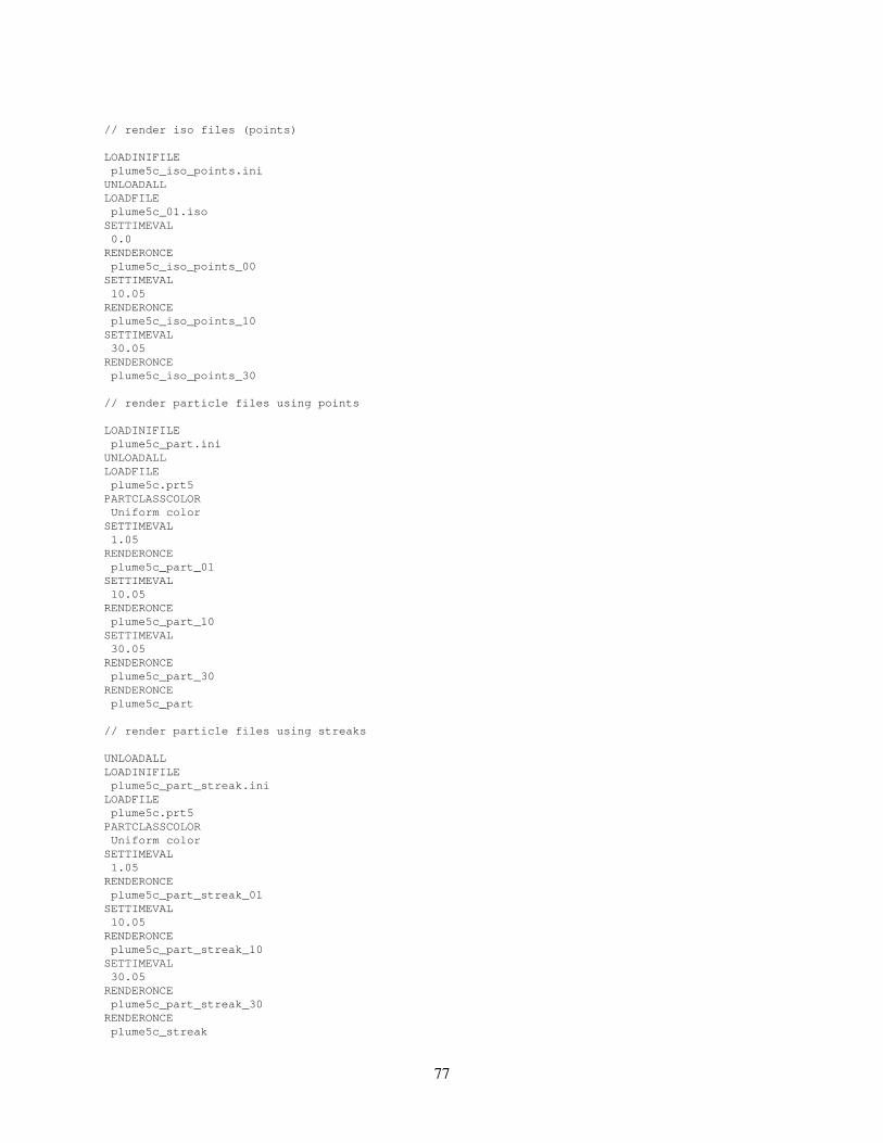
Figure 2.7 presents images verifying the display of particles and streaks. Images are drawn at 1 s, 10 s and30 s. The first column shows particles while the second and third columns shows streaks with duration 0.5 sand 1 s. Streaks are a good way of visualizing motion in a still image (i.e., on paper) since the streak showsa history of where the particle has been.

12

points 0.5 s streaks 1 s streaks

Figure 2.7: A test showing particles and particle streaks at 1 s, 10 s and 30 s

13

2.4 Slices

Figure 2.8 presents images verifying the display of node centered data slices. Images are drawn at 0 s,10 s and 30 s. A portion of the interior gas temperature is initialized to 600 ◦C corresponding to the redrectangular block appearing in the first row. The first column visualizes all of the data in the slice. Thesecond column discards or chops data below 140 ◦C. Note that the color near the chopped boundary shouldmatch the color in the color bar near 140 ◦C.

Figures 2.9 and 2.10 present images verifying the display of cell centered data. Images in Fig. 2.9 aredrawn at 0 s, 10 s and 30 s. Images in Fig. 2.10 tests the transfer of data from FDS to Smokeview.

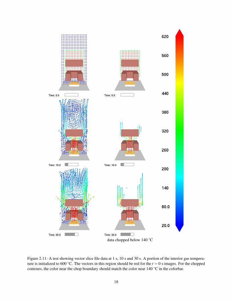
Figure 2.11 present images verifying the display of vector slices. Again, vector slice file images aredrawn at 0 s, 10 s and 30 s. The first column draws all vectors while the second column discards or chopsvectors below 140 ◦C.

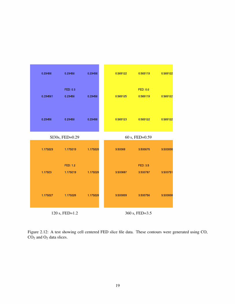
Figure 2.12 presents slice file images verifying the computation of fractional effective dose (FED). FEDis a measure of human incapacitation or hazard due to combustion gases[8]. Images are drawn at 30 s, 60 sand 120 s and 240 s. The FED is computed using three data slices with concentration of 1000 ppm for COand volume fractions of 0.02 and 0.07 for CO2 and O2 respectively. These values result in FED values of1.5 at 30 s, 3.0 at 60 s, 6.0 at 120 s and 12.0 at 240 s.

Figure 2.13 presents images of 3D slices oriented in two different ways. Images are drawn at 0 s, 10 sand 30 s.

Figure 2.14 presents images from data differenced by Smokediff. Smokediff computed the differencebetween two similar FDS cases and generated slice files. Difference contours from these slice files aredisplayed at 0 s, 10 s and 15 s.

14

node centered data node centered chopped data

Figure 2.8: A test showing shaded and chopped contours of node centered slice file data at 0 s, 10 s and 30 s.A portion of the interior gas temperature is initialized to 600 ◦C. The slice file in this region should be redfor the t = 0 s images. For the chopped contours, the color near the chop boundary should match the colornear 140 ◦C in the colorbar.

15

cell centered data cell centered chopped data

Figure 2.9: A test showing shaded and chopped contours of cell centered slice file data at 0 s, 10 s and 30 s.A portion of the interior gas temperature is initialized to 600 ◦C. The slice file in this region should be redfor the t = 0 s images. For the chopped contours, the color near the chop boundary should match the colornear 140 ◦C in the colorbar.

16

a) plan view (top slice) b) 3D view

c) elevation view (front slice) d) side view (right slice)

Figure 2.10: A test to demonstrate that cell centered slice file data is transferred to Smokeview properly.Cell values are initialized in FDS to 100∗ i+10∗ j+k where 1≤ i≤ 3, 1≤ j≤ 4 and 1≤ k≤ 5. Cell valuesdisplayed should match the (i, j,k) grid cell indices. The three plots in the 3D view correspond to the plan,elevation and side view plots. 17

data chopped below 140 ◦C

Figure 2.11: A test showing vector slice file data at 1 s, 10 s and 30 s. A portion of the interior gas tempera-ture is initialized to 600 ◦C. The vectors in this region should be red for the t = 0 s images. For the choppedcontours, the color near the chop boundary should match the color near 140 ◦C in the colorbar.

18

SI30s, FED=0.29 60 s, FED=0.59

120 s, FED=1.2 360 s, FED=3.5

Figure 2.12: A test showing cell centered FED slice file data. These contours were generated using CO,CO2 and O2 data slices.

19

general orientation second orientation

Figure 2.13: A test showing arbitrarily oriented slice file planes generated from 3D slice files at 0 s, 10 s and30 s. Two orientations are shown at three time steps.

20

Figure 2.14: A test showing slice contours generated by differencing two cases with Smokediff at 0 s, 10 sand 30 s.

21

Figure 2.15: A test showing 3D smoke drawn at 1 s, 10 s and 30 s

2.5 3D Smoke

Figure 2.15 presents images verifying the display of 3D smoke and fire (heat release rate per unit volumeor HRRPUV). A series of 3D smoke images are drawn at 1 s, 10 s and 30 s. The images contain semi-transparent slices derived from both soot density and HRRPUV data.

22

step contours continuous contours

Figure 2.16: A test showing PLOT3D stepped and continuous temperature contours.

2.6 Plot3D

Figure 2.16 presents images verifying the display of PLOT3D contours. Three types of contours are avail-able for visualizing PLOT3D data: stepped, continuous and narrow band. This figure shows stepped andcontinuous contours. Figure 2.17 shows stepped contours in at four positions along the y axis. Figure 2.18shows narrow band contours at four positions front to back. Figure 2.19 shows velocity vectors at the samefour positions as in Figure 2.17. Figure 2.20 shows PLOT3D iso-surfaces for 50 ◦C, 230 ◦C, 410 ◦C and590 ◦C.

visualizing the motion of a fire across the simulation. The fire line slice is formed by setting the min andmax temperature bounds to 20 ◦C and 200 ◦C respectively and chopping data below 150◦C. The fire line slicefile can then be made very small using Smokezip to compress it. Fire line images are drawn at 10 s, 20 s,30 s and 40 s. The fire lines conform to the hill going through the middle of the scene. fire_line.ssf.

follows the terrain as

23

Figure 2.17: A test showing PLOT3D stepped contours at four positions along the y axis.

24

Figure 2.18: A test showing PLOT3D narrow band contours at four positions along the y axis.

25

Figure 2.19: A test showing PLOT3D vectors shaded by temperature at four positions along the y axis.

26

50 ◦C 230 ◦C

410 ◦C 590 ◦C

Figure 2.20: A test showing PLOT3D iso-surfaces for 50 ◦C, 230 ◦C, 410 ◦C and 590 ◦C.

27

28

Chapter 3

Smoke Visualization Tests

Correct smoke visualization requires that smoke flow be both computed and drawn correctly. The FDS Veri-fication Guide [7] addresses computation in terms of soot/smoke production, transport, etc. A verification ofhow smoke is drawn is addressed in this chapter. More precisely, given a known density and distribution ofsoot, does the smoke drawn by Smokeview match how theory predicts it should appear. Presently, the maininterest is in how smoke obscures objects in the background. Visualization effects due to light scattering arenot modeled except to consider the smoke albedo when drawing its grey level.

The smoke drawing verification problem is partitioned into two steps. The first step, documented inSection 3.1, is to verify that Smokeview can record the correct grey level of smoke as it is drawn on thescreen. This step is necessary because screen colors, in this case the smoke obscuration levels to be verified,are not directly accessible to Smokeview. They must be retrieved from the video card buffers. The secondstep, documented in Section 3.2, is to verify that Smokeview can draw the correct shade of grey given aknown soot density level within the scene.

3.1 Recording Smoke Levels

Smokeview does not have direct access to colors drawn on the screen. Smokeview passes vertex colors tothe video driver. The video driver in turn fills in interpolated colors within these vertices. To obtain thesecolors, Smokeview must ‘read’ them back in after they are drawn. A further complication is that smoke isdrawn in Smokeview using a physical coordinate system. The smoke opacity levels are retrieved using thescreen coordinate system, ie. at particular pixel locations. It is this transformation process, from physical toscreen coordinates, that is verified in this step.

In the case of 3D smoke visualization, these colors represent smoke opacity levels. To obtain theselevels and thereby verifying that they are correct, Smokeview makes use of a special sensor or device namedsmoke_sensor which Smokeview uses to obtain color values at the sensor location. This device behaves likeother FDS devices but has the additional property that when used by Smokeview, it displays the grey levelas viewed by the observer. This grey level is displayed as a number between 0 and 255.

The user places a device of type smoke_sensor at a particular (x,y,z) location. Smokeview displaysthe sensor as a white disk with color (255,255,255) always oriented towards the observer. When drawingsmoke that resides between the sensor and the observer (your eye), the smoke sensor is partially obscuredby the smoke. Smokeview then alters the smoke sensor color according to how much and how thick theintervening smoke is. It does this by blending each smoke plane one plane at a time using the color andopacity levels of that plane. The grey level is simply Smokeview’s computation of the integrated smokethickness along a path between the sensor location and the eye. The colors displayed are the result computa-tions performed by the video card using OpenGL, the graphics library used by Smokeview to visualize FDS

29

Figure 3.1: A test verifying that Smokeview can correctly transform the physical (x,y,z) location of thesmoke_sensor object to its equivalent screen coordinates where the underlying smoke obscuration level isretrieved. A small white (255,255,255) smoke_sensor appears in front of a grey (128,128,128) obstacle. Thevalue displayed should be 255, the value recorded by Smokeview. If the physical to screen transformationis performed incorrectly a value of 128 will be displayed (since it will pick up a color elsewhere).

scenarios.Figure 3.1 illustrates an initial test of this process. It verifies that Smokeview can transform the sensor

location from physical ‘FDS’ coordinates to screen coordinates (pixel locations) and further can correctlyrecord the grey level at those screen coordinates even when surrounded by other objects with different colors.In this case, the smoke sensor is white and there is no intervening smoke. The background is a neutral greywith grey level of 128. The value displayed over the sensor then should always be 255 not 128 no matterhow the scene is oriented. If Smokeview made an error determining the sensor screen coordinates the greylevel displayed would be 128 (grey level of the adjacent grey background) not 255 (grey level of the sensor).

Figure 3.2 shows two colorbars, both containing shades of grey. One shows white and near-white shades,the other shows black and near black shades. This figure illustrates the difficulty one has in distinguishingnearly equal shades and by inference the difficulty in distinguishing two smoke scenes drawn using nearlythe same amounts of smoke. When comparing a computed smoke shade with the actual (as in Figure 3.4)one must keep in mind the eye’s inability to distinguish nearly equal shades of grey.

3.2 Verifying Smoke Levels

Smoke levels are verified in Smokeview by setting up an FDS case with a constant smoke density throughoutthe domain. A smoke density S = 79.67 mg/m3 and mass extinction coefficient K = 8700 m2 are chosen inEq. 3.1 to generate opacity levels 192, 128, 64, 32, 16 and 8 at path lengths ∆x= 0.4 m,1 m,2 m,3 m,4 m,5 m

α = 255 exp(−K S∆x) (3.1)

where α is a scaled opacity (from 0 to 255 rather than the usual 0 to 1).Figure 3.3 shows a side view of the numerical smoke box used to perform this test. In addition to the

walls surrounding the box, this box consists of six parallel walls within the box spaced 1.0 m apart. The

30

128192 3264 816

0 42 86 1610 24 32

255 251253 239245 231 223247249

128192 3264 816

0 42 86 1610 24 32

255 251253 239245 231 223247249

Figure 3.2: Shade of grey resolution test. The number within each square represents the shade of grey usedto color that square, 0 for black and 255 for white. Adjacent squares are drawn with nearly equal shadestesting the ability of sensors such as the eye, computer monitor or the printed page to distinguish them.

widths increase from one wall to the next (from front to back) so that when looking at the box from the fronta different distance or path length occurs between the observer and the portion of the wall that is visible.Again, the spacing between the walls, the distance between the walls and the observer and the initial sootdensities is chosen so that the computed smoke obscurations work out to nice values.

Figure 3.4 shows quantitative tests of the smoke opacity calculation performed in Smokeview for twodifferent FDS grid resolutions and three different skip levels1. This figure also gives the predicted shadesof grey based upon the specified soot densities, mass extinction coefficient and path lengths. The smokevisualization algorithm is verified then if the shades of grey in the Smokeview visualizations match thecorresponding predicted shades of grey. Each shaded rectangle is accompanied by a numerical value thatcan also be used to judge whether the visualization is verified.

The numbers displayed in this Fig. 3.4 represent the shade of the underlying rectangle. These numbersmay be verified by using a program such as Adobe Photoshop to examine the pixel values of this rectangularregion. The numbers are verified when they match the pixel values as reported by Photoshop or any otherprogram that can report image values.

When soot densities are constant, smoke grey level or opacity, α may be computed by using Eq. (3.1).Solving Eq. (3.1) for ∆x gives

∆x =− ln(α/255)K S

(3.2)

Path lengths (smoke sensor locations) are chosen to obtain grey levels, α , of 192, 128, 64, 32, 16 and 8.These path lengths may be found by substituting these grey levels into Eq. (3.2) to obtain ∆x values of0.41 m, 1.0 m, 2.0 m, 3.0 m, 4.0 m and 5.0 m respectively. The walls in smoketest2.fds are placed atthese distances from the front of the simulation domain. Comparing the Smokeview generated smoke levelswith theoretical values one finds as expected that better results are achieved when using a more refined grid(0.1 m rather than 0.2 m) and using all planes (no skipping).

1Smokeview allows one to skip grid planes when visualizing smoke. The smoke opacity is adjusted by Smokeview to accountfor the skips.

31

Figure 3.3: Side view of the numerical smoke test compartment. Walls are placed at 0.4 m, 1 m, 2 m, 3 m,4 m , 5 m from the front to make the theoretical grey levels work out to 192, 128, 64, 32, 16 and 8.

32

planes 0.1 m grid 0.2 m grid

all

every 2nd

every 3rd

theoretical

Figure 3.4: A test verifying the smoke opacity calculation. This test simplifies the general case by assuminga uniform distribution of smoke. The test is repeated for two grid resolutions and three grid spacings. TheFDS input file is set up to result in theoretical grey levels of 8, 16, 32, 64, 128 and 192 for the differentregions of the test.

33

34

Chapter 4

WUI Test Cases

This chapter presents techniques added to Smokeview [2] applicable for visualizing WUI (wildland urbaninterface) and wild fire scenarios. Two techniques involve 1) visualizing changing terrain using satelliteimages with modeling results overlayed and 2) making use of geometric objects for representing modelingelements such as trees or building structures. These two techniques use data generated by fire models such asFDS [9] or WFDS (FDS revision 9977)[10]. A third technique involves visualizing experimentally deriveddata rather than modeling data. Wind sensor data is visualized using flow vectors along with visual indicatorsof data uncertainty. Smokeview images are displayed in the following figures to illustrate these techniques.

4.1 FDS Cases

The figures in this section were generated with FDS revision 16557 . Figure 4.1 presents contours of a levelset computation. The level set contours are drawn on a sloped terrain. These level set contours representa fire line. A fire line is used with wildland fire simulations as an efficient method for visualizing themotion of a fire across the simulation. A fire line in the context of Smokeview is just a special case of atemperature slice contour. The thin red line represents the location where burning is currently taking place.The grey region represents where burning has occurred and the green region represents where burning hasnot occurred. Level sets are used to quickly (relative to a complete computational fluid dynamic calculation) model fire spread and fire line locations. In this particular case, images are drawn at 30 s, 60 s, 90 s and120 s. The test verifies that the level set slices follow the sloped terrain. Figure 4.2 and 4.3 also presentimages of level set contours. These contour slices are drawn along with a satellite image of the region beingmodeled.

Figure 4.4 presents images of temperature contours drawn on a terrain geometry. The scenario consistsof a small hill parallel to the vertical axis of the scene. Images are drawn at 15 s, 30 s, 45 s and 60 s. The testverifies that temperature contours follow the sloped terrain and that the red blockage (a non-terrain blockagerepresenting a structure) is drawn correctly along with the terrain.

Smokeview typically visualizes data generated by software such as FDS [9], CFAST [11] or WFDS[10].Figure 4.5 presents a visualization of data obtained from wind measuring sensors rather than simulationdata. Smokeview can use the wind sensor data to visualize velocity profiles and variability and uncertaintypresent in the experimental data. The vertical array of green spheres represent the measurement locations.The distance from these spheres to the green or red spherical shells gives a relative measure of the windspeed. The shell diameter gives a measure of the wind direction measurement uncertainty. Likewise the

35

30 s 60 s

90 s 120 s

Figure 4.1: A test showing level set slices drawn along a sloped terrain at 30 s, 60 s, 90 s and 120 s. The testverifies that level set slices follow the sloped terrain. The thin red line represents where burning is currentlytaking place. The grey and green regions represent where burning has and has not occurred respectively.

36

0 s 300 s

600 s 900 s

1200 s 1500 s

Figure 4.2: A test showing a fire line slice drawn along a sloped and textured terrain at 0 s, 300 s, 600 s,900 s, 1200 s, and 1500 s of simulated time. The test verifies that the level set slices follow the slopedterrain.

37

Figure 4.3: A test showing a fire line slice drawn along a sloped and textured terrain at 1800 s simulatedtime.

38

15 s 30 s

45 s 60 s

Figure 4.4: A test showing temperature slices drawn along a sloped terrain at 15 s, 30 s, 45 s and 60 s.The test verifies that the temperature slices follow the sloped terrain and that the non-terrain red blockage(representing a structure) is drawn with the terrain.

39

shell thickness give a measure of the wind velocity measurement uncertainty.

40

Figure 4.5: A test showing wind vectors drawn using data obtained from a wind sensor. The line segmentsrepresent wind speed and direction. The spherical shells represent uncertainty in wind direction (shelldiameter) and wind speed (shell thickness).

41

Figure 4.6: A test showing trees drawn as Smokeview objects. The tree canopy is colored green drawn as acone, the tree trunk is colored brown drawn as a cylinder.

state 1 state 2 state 3 state 4

Figure 4.7: A test showing four states of the smokeview trunk and canopy objects. The states are unburnedtrunk and canopy, burned trunk and canopy, burned trunk (canopy burned away), both canopy and trunkburned away.

4.2 WFDS Cases

The figures in this section were created using data generated by WFDS (FDS svn revision 9977). Figure 4.6shows an example of trees drawn as Smokeview objects. The tree is drawn as a cylinder colored brown anda cone colored green. Tree objects may change appearance as a simulation progresses as illustrated in Fig.4.7. Tree states are a normal view, partially burned, partially burned (canopy burned away) and completelyburned.

Figure 4.8 shows an example of trees drawn as particles. Particle represent small units of fuel. Particlecolor represents temperature. As particles use up fuel they disappear. When many trees are simulated, itis difficult to discern individual trees when drawn as particles. Fig. 4.9 shows an equivalent view usingan isosurface. The isosurface location is determined from the boundary (between particle and non-particleregions in the simulation) of the particle cloud shown in Fig. 4.8. Figure 4.10 show a particle file drawnusing canopy objects. The objects are colored according to the particle color as computed by FDS.

42

0 s

20 s

40 s

60 s

Figure 4.8: A test showing trees drawn as particles at 0 s, 20 s, 40 s and 60 s. Particle represent small unitsof fuel. Particle color represents temperature. As particles use up fuel they disappear.

43

0 s

20 s

40 s

60 s

Figure 4.9: A test showing trees drawn as isosurface at 0 s, 20 s, 40 s and 60 s. The surface location isdetermined from the boundary of the particle cloud shown in Fig. 4.8.

44

Figure 4.10: A test showing particles drawn as canopy objects at 0 s, 3 s, 6 s and 9 s. The canopy is coloredaccording to temperature.

45

46

Chapter 5

Other Tests

5.1 Obstacles

Figures 5.1 and 5.2 test different methods for displaying obstacles. Figure 5.1 shows obstacles drawn assolids, as outlines or hidden. Figure 5.2 shows obstacles drawn transparently. The left view shows theopaque obstacle drawn in front (and blocking) a portion of the transparent obstacle behind. The centerview shows both obstacles unobscured. The right view shows the transparent blockage drawn in front withthe opaque blockage visible behind. The images for this test were created automatically by running theSmokeview script, plume5c.ssf (see Appendix B.4).

47

solid view of obstacles outline view of obstacles obstacles hidden

Figure 5.1: A test showing 3 drawing modes for representing blockages: solid, outline and hidden

left view - opaque obstacle in front center view - both obstacles visible right view - transparent obstacle in front

Figure 5.2: A test showing that transparent objects are drawn properly

48

Figure 5.3: A test showing that devices are drawn properly

5.2 Devices

The case illustrated in Fig. 5.3 tests how well Smokeview can display many devices. This figure shows aseries of sprinklers with three different levels of detail. Smokeview should be able to smoothly rotate thisscene on computers with good video cards. The images for this test were created automatically by runningthe Smokeview script, sprinkler_many.ssf (see Appendix B.9).

49

show all vents hide open vents hide all vents

Figure 5.4: A test showing 3 modes for drawing vents: show all vents, hide open vents and hide all vents

5.3 Vents

Figure 5.4 tests vent display. This figure shows three different levels of vent visibility: all vents displayed,only non-open vents displayed and all vents hidden. The images for this test were created automaticallyby running the Smokeview script, plume5c.ssf (see Appendix B.4). Figure 5.5 shows circular ventsdrawn on the sides of a blockage. The circular vents are drawn as requested by the user (a circle) and asimplemented within FDS. Figure 5.6 shows circular vents drawn on exterior boundary. The circular ventsare drawn as requested by the user (a circle) and as implemented within FDS.

50

user specification FDS implementation

Figure 5.5: A test showing circular vents drawn as specified in the input file and as implemented withinFDS. The circular vents are applied to a blockage.

51

user specification FDS implementation

Figure 5.6: A test showing circular vents drawn as specified in the input file and as implemented withinFDS. The circular vents are applied to the external boundary.

52

5.4 Conversion to Color

Smokeview converts data values obtained from an FDS calculation to color using a linear scaling of the form

Ci = 255Vi−Vmin

Vmax−Vmin(5.1)

where Ci is an index into a color table between 0 and 255, Vmin and Vmax are data bounds, and Vi is a datavalue to be converted. Figure 5.7 presents images verifying the conversion of data to colors. The input file,colorconv.fds (see Appendix A.2), was set up so that initially the left half of the domain (it is a 2Dcase) is 20 ◦C and the right half is 100 ◦C. The images for this test were created automatically by runningthe Smokeview script, colorconv.ssf (see Appendix B.2).

A second color conversion test involves the use of the colorbar to highlight portions of the data. Thecase was set up so that the vertical slice aligns with the colorbar. The gas temperatures were defined toincrease from 20 ◦C to 100 ◦C from the floor to the ceiling. As a result, when one selects the colorbar, theselected region in the colorbar should match the selected region in the vertical slice. The images for this testwere created automatically by running the Smokeview script, colorbar.ssf (see Appendix B.1).

53

Figure 5.7: A test showing that data is converted to color properly. Temperature between 20 ◦C and 100 ◦Care converted to colors between blue and red.

54

Figure 5.8: A test showing that data is converted to color properly. Temperature between 20 ◦C and 100 ◦Care converted to colors between blue and red. The highlighted region in the colorbar matches the highlightedregion in the vertical slice.

55

5.5 GPU Test

Figure 5.9 tests whether Smokeview produces similar images when using the GPU and CPU for drawing 3Dsmoke. The first column shows CPU generated images at 5 s, 10 s and 30 s while the second column showsGPU generated images at the same times. The corresponding images in each column should be similar.

56

CPU generated GPU generated

Figure 5.9: A test showing that the GPU is properly used to draw smoke

57

58

Bibliography

[1] G.P. Forney. Smokeview (Version 6), A Tool for Visualizing Fire Dynamics Simulation Data, VolumeI: User’s Guide. NIST Special Publication 1017-1, National Institute of Standards and Technology,Gaithersburg, Maryland, May 2013. i, 1

[2] G.P. Forney. Smokeview (Version 6), A Tool for Visualizing Fire Dynamics Simulation Data, VolumeII: Technical Reference Guide. NIST Special Publication 1017-2, National Institute of Standards andTechnology, Gaithersburg, Maryland, May 2013. i, 1, 35

[3] G.P. Forney. Smokeview (Version 6), A Tool for Visualizing Fire Dynamics Simulation Data, Vol-ume III: Verification Guide. NIST Special Publication 1017-3, National Institute of Standards andTechnology, Gaithersburg, Maryland, May 2013. i

[4] K. McGrattan, S. Hostikka, R. McDermott, J. Floyd, C. Weinschenk, and K. Overholt. Fire DynamicsSimulator, User’s Guide. National Institute of Standards and Technology, Gaithersburg, Maryland,USA, and VTT Technical Research Centre of Finland, Espoo, Finland, sixth edition, September 2013.i, 1

[5] K. McGrattan, S. Hostikka, R. McDermott, J. Floyd, C. Weinschenk, and K. Overholt. Fire DynamicsSimulator, Technical Reference Guide, Volume 1: Mathematical Model. National Institute of Stan-dards and Technology, Gaithersburg, Maryland, USA, and VTT Technical Research Centre of Finland,Espoo, Finland, sixth edition, September 2013. i, 1

[6] W. W. Jones, R. D. Peacock, G. P. Forney, and P. A. Reneke. CFAST, Consolidated Model of FireGrowth and Smoke Transport (Version 5. technical reference guide. NIST Special Publication 1030,National Institute of Standards and Technology, Gaithersburg, Maryland, October 2004. 1

[7] K. McGrattan, S. Hostikka, R. McDermott, J. Floyd, C. Weinschenk, and K. Overholt. Fire DynamicsSimulator, Technical Reference Guide, Volume 2: Verification. National Institute of Standards andTechnology, Gaithersburg, Maryland, USA, and VTT Technical Research Centre of Finland, Espoo,Finland, sixth edition, September 2013. 1, 29

[8] D.A. Purser. SFPE Handbook of Fire Protection Engineering, chapter Toxicity Assessment of Com-bustion Products. National Fire Protection Association, Quincy, Massachusetts, 3rd edition, 2002.14

[9] K. McGrattan, S. Hostikka, R. McDermott, J. Floyd, C. Weinschenk, and K. Overholt. Fire Dynam-ics Simulator, Technical Reference Guide. National Institute of Standards and Technology, Gaithers-burg, Maryland, USA, and VTT Technical Research Centre of Finland, Espoo, Finland, sixth edition,September 2013. Vol. 1: Mathematical Model; Vol. 2: Verification Guide; Vol. 3: Validation Guide;Vol. 4: Configuration Management Plan. 35

59

[10] W. Mell, A. Maranghides, R. McDermott, and S. Manzello. Numerical simulation and experiments ofburning Douglas fir trees. Combustion and Flame, 156:2023–2041, 2009. 35

[11] R. D. Peacock, G. P. Forney, and P. A. Reneke. CFAST – Consolidated Model of Fire Growth andSmoke Transport (Version 6): Technical Reference Guide. Special Publication 1026, National Instituteof Standards and Technology, Gaithersburg, Maryland, July 2011. 35

60

Appendix A

Input Files

A.1 colorbar&HEAD CHID='colorbar', TITLE='Test of colorbar selection' /REM This test case is used to test Smokeview's ability toREM correctly select the colorbar and shade the appropriateREM region black.

REM To do this,REM 1) press "g" to turn on the grid.REM 2) "Page Up" and put a horizonal grid slice "somewhere"REM 3) select the colorbar, centering the resulting black bandREM on the horizontal grid plane. Note the value.REM 4) Use the File/BOunds dialog box to change the min and or maxREM setting for the temperature slice file.REM 5) repeaset setp 3. Value noted should remain the same.

&MESH IJK=20,10,10, XB=0.0,2.0,0.0,1.0,0.0,1.0 /

&TIME T_END=10.0 /

&MISC LAPSE_RATE=10.0, TMPA=10. /

&RADI RADIATION=.FALSE./

&SLCF PBY=0.6, QUANTITY='TEMPERATURE' /

&VENT MB='XMAX', SURF_ID='OPEN' /&VENT MB='YMAX', SURF_ID='OPEN' /&VENT MB='ZMAX', SURF_ID='OPEN' /&VENT MB='XMIN', SURF_ID='OPEN' /&VENT MB='YMIN', SURF_ID='OPEN' /&VENT MB='ZMIN', SURF_ID='OPEN' /

&TAIL /

A.2 colorconvA simple two-dimensional case testing data to color conversion

&HEAD CHID='colorconv', TITLE='Test data to color conversion, SVN $Revision: 12143 $' /&DUMP NFRAMES=800 /

&MESH IJK=100,1,100, XB=0.0,100.0,-1.0,1.0,0.0,100.0 /&SURF ID='COOLWALL' TMP_FRONT=20.0 /

61

&SURF ID='HOTWALL' TMP_FRONT=100.0 /&SURF ID='INSWALL' ADIABATIC=.TRUE. /&MISC FLUX_LIMITER=4, CFL_VELOCITY_NORM=1, CHECK_VN=.FALSE. /

&TIME T_END=200.0 /

&RADI RADIATION=.FALSE. /&INIT XB= 0.0, 50.0,-2.0,2.0,0.0,100.0, TEMPERATURE=20. /&INIT XB=50.0,100.0,-2.0,2.0,0.0,100.0, TEMPERATURE=100. /

&VENT XB= 0.0, 100.0, -1.0, 1.0, 0.0, 0.0, SURF_ID='COOLWALL' /&VENT XB= 0.0, 100.0, -1.0, 1.0, 100.0, 100.0, SURF_ID='HOTWALL' /&VENT XB= 0.0, 0.0, -1.0, 1.0, 0.0, 100.0 SURF_ID='INSWALL' /&VENT XB= 100.0, 100.0, -1.0, 1.0, 0.0, 100.0 SURF_ID='INSWALL' /

&SLCF PBY=0.0, QUANTITY='TEMPERATURE' /

&TAIL /

A.3 fed_test&HEAD CHID='fed_test', TITLE='Check FED computation in smokeview, SVN $Revision: 12143 $'/

&MESH XB=0.0,1.0,0.0,1.0,0.0,1.0, IJK=3,3,3 /

&TIME T_END=360.0, DT=0.1 /&DUMP NFRAMES=2880 /

&SPEC ID='NITROGEN', BACKGROUND=.TRUE. /&SPEC ID='OXYGEN' /&SPEC ID='CARBON DIOXIDE' /&SPEC ID='CARBON MONOXIDE'/

&INIT XB=0.0,1.0,0.0,1.0,0.0,1.0MASS_FRACTION(1)=0.078322, SPEC_ID(1)='OXYGEN',MASS_FRACTION(2)=0.030769,SPEC_ID(2)='CARBON DIOXIDE'MASS_FRACTION(3)=0.000979,SPEC_ID(3)='CARBON MONOXIDE' /

&DEVC ID='DEV1A', XYZ=0.5,0.5,0.6, QUANTITY='FED' /

&SLCF PBY=0.5,QUANTITY='VOLUME FRACTION' SPEC_ID='CARBON DIOXIDE' /&SLCF PBY=0.5,QUANTITY='VOLUME FRACTION' SPEC_ID='CARBON MONOXIDE' /&SLCF PBY=0.5,QUANTITY='VOLUME FRACTION' SPEC_ID='OXYGEN' /&SLCF PBY=0.5,QUANTITY='VOLUME FRACTION' SPEC_ID='CARBON DIOXIDE', CELL_CENTERED=.TRUE. /&SLCF PBY=0.5,QUANTITY='VOLUME FRACTION' SPEC_ID='CARBON MONOXIDE', CELL_CENTERED=.TRUE. /&SLCF PBY=0.5,QUANTITY='VOLUME FRACTION' SPEC_ID='OXYGEN', CELL_CENTERED=.TRUE. /

&TAIL /

A.4 plume5c&HEAD CHID='plume5c',TITLE='Plume whirl case SVN $Revision: 14561 $' /

same as plume5a except there is a blockage in the middle of the scene to block the flowThe purpose of this case is to demonstrate the curved flow (via streak lines) that results.

&MESH IJK=16,16,32, XB=0.0,1.6,0.0,1.6,0.0,3.2 /

&MISC HRRPUV_MAX_SMV=1300.0 /

&DUMP NFRAMES=400 DT_PL3D=8.0, DT_SL3D=0.1 /

&INIT XB=0.2,1.4,0.2,1.4,0.5,2.2 TEMPERATURE=600.0 /

62

&TIME T_END=40. / Total simulation time

&MATL ID = 'FABRIC'FYI = 'Properties completely fabricated'SPECIFIC_HEAT = 1.0CONDUCTIVITY = 0.1DENSITY = 100.0N_REACTIONS = 1NU_SPEC = 1.SPEC_ID = 'PROPANE'REFERENCE_TEMPERATURE = 350.HEAT_OF_REACTION = 3000.HEAT_OF_COMBUSTION = 15000. /

&MATL ID = 'FOAM'FYI = 'Properties completely fabricated'SPECIFIC_HEAT = 1.0CONDUCTIVITY = 0.05DENSITY = 40.0N_REACTIONS = 1NU_SPEC = 1.SPEC_ID = 'PROPANE'REFERENCE_TEMPERATURE = 350.HEAT_OF_REACTION = 1500.HEAT_OF_COMBUSTION = 30000. /

&SURF ID = 'UPHOLSTERY_LOWER'FYI = 'Properties completely fabricated'RGB = 151,96,88BURN_AWAY = .FALSE.MATL_ID(1:2,1) = 'FABRIC','FOAM'THICKNESS(1:2) = 0.002,0.1

/

&SURF ID = 'UPHOLSTERY_UPPER'FYI = 'Properties completely fabricated'RGB = 151,96,88BURN_AWAY = .FALSE.TMP_FRONT = 600.0

/&REAC C=3,H=8,SOOT_YIELD=0.01,FUEL='PROPANE'/&SURF ID='BURNER',HRRPUA=600.0,PART_ID='tracers' / Ignition source

&VENT XB=0.5,1.1,0.5,1.1,0.1,0.1,SURF_ID='BURNER' / fire source on kitchen stove

&OBST XB=0.5,1.1,0.5,1.1,0.0,0.1 /&OBST XB=0.3,1.3,0.3,1.3,0.4,0.8 SURF_ID='UPHOLSTERY_LOWER'/&HOLE XB=0.6,1.0,0.2,0.8,0.3,0.9 /&OBST XB=0.3,1.3,0.3,1.3,1.2,1.6 SURF_ID='UPHOLSTERY_UPPER' /

&VENT XB=0.0,1.6,0.0,0.0,0.0,3.2,SURF_ID='OPEN'/&VENT XB=1.6,1.6,0.0,1.6,0.0,3.2,SURF_ID='OPEN'/&VENT XB=0.0,1.6,1.6,1.6,0.0,3.2,SURF_ID='OPEN'/&VENT XB=0.0,0.0,0.0,1.6,0.0,3.2,SURF_ID='OPEN'/&VENT XB=0.0,1.6,0.0,1.6,3.2,3.2,SURF_ID='OPEN'/

&ISOF QUANTITY='TEMPERATURE',VALUE(1)=100.0 / Show 3D contours of temperature at 100 C&ISOF QUANTITY='TEMPERATURE',VALUE(1)=200.0 / Show 3D contours of temperature at 200 C&ISOF QUANTITY='TEMPERATURE',VALUE(1)=620.0 / Show 3D contours of temperature at 620 C&ISOF QUANTITY='TEMPERATURE',VALUE(1:2)=200.0,400.0 / Show 3D contours of temperature at 200 C

&PART ID='tracers',MASSLESS=.TRUE.,QUANTITIES(1:4)='U-VELOCITY','V-VELOCITY','W-VELOCITY'SAMPLING_FACTOR=10 / Description of massless tracer particles. Apply at a

solid surface with the PART_ID='tracers'

X slices

63

&SLCF PBX=0.8,QUANTITY='TEMPERATURE',VECTOR=.TRUE. / Add vector slices colored by temperature&SLCF PBX=0.8,QUANTITY='TEMPERATURE',CELL_CENTERED=.TRUE. /

Y slices

&SLCF PBY=0.8,QUANTITY='TEMPERATURE',VECTOR=.TRUE. /&SLCF PBY=0.8,QUANTITY='VOLUME FRACTION' SPEC_ID='PROPANE' /&SLCF PBY=0.8,QUANTITY='VOLUME FRACTION' SPEC_ID='OXYGEN' /&SLCF PBY=0.8,QUANTITY='VOLUME FRACTION' SPEC_ID='CARBON DIOXIDE' /&SLCF PBY=0.8,QUANTITY='VOLUME FRACTION' SPEC_ID='CARBON MONOXIDE' /&SLCF PBY=0.8,QUANTITY='TEMPERATURE',CELL_CENTERED=.TRUE. /

Z slices

&SLCF PBZ=0.4,QUANTITY='TEMPERATURE',VECTOR=.TRUE. /&SLCF PBZ=0.4,QUANTITY='TEMPERATURE',CELL_CENTERED=.TRUE. /&SLCF PBZ=1.6,QUANTITY='TEMPERATURE',VECTOR=.TRUE. /&SLCF PBZ=1.6,QUANTITY='TEMPERATURE',CELL_CENTERED=.TRUE. /&SLCF PBZ=3.2,QUANTITY='TEMPERATURE',VECTOR=.TRUE. /&SLCF PBZ=3.2,QUANTITY='TEMPERATURE',CELL_CENTERED=.TRUE. /

3d slices

&SLCF XB=0.0,1.6,0.0,1.6,0.0,3.2,QUANTITY='TEMPERATURE' ,VECTOR=.TRUE. /&SLCF XB=0.0,1.6,0.0,1.6,0.0,3.2, QUANTITY='TEMPERATURE',CELL_CENTERED=.TRUE. / 3D slice&SLCF XB=0.0,1.6,0.0,1.6,0.0,3.2,QUANTITY='VOLUME FRACTION' SPEC_ID='CARBON DIOXIDE' /&SLCF XB=0.0,1.6,0.0,1.6,0.0,3.2,QUANTITY='VOLUME FRACTION' SPEC_ID='CARBON MONOXIDE' /&SLCF XB=0.0,1.6,0.0,1.6,0.0,3.2,QUANTITY='VOLUME FRACTION' SPEC_ID='OXYGEN' /&SLCF XB=0.0,1.6,0.0,1.6,0.0,3.2, QUANTITY='DENSITY',SPEC_ID='SOOT',CELL_CENTERED=.TRUE. / 3D slice&SLCF PBY=1.6,QUANTITY='VOLUME FRACTION' SPEC_ID='CARBON DIOXIDE' /&SLCF PBY=1.6,QUANTITY='VOLUME FRACTION' SPEC_ID='CARBON MONOXIDE' /&SLCF PBY=1.6,QUANTITY='VOLUME FRACTION' SPEC_ID='OXYGEN' /

&BNDF QUANTITY='GAUGE HEAT FLUX' / Common surface quantities. Good for monitoring fire spread.&BNDF QUANTITY='BURNING RATE' /&BNDF QUANTITY='WALL TEMPERATURE' /&BNDF QUANTITY='WALL TEMPERATURE' CELL_CENTERED=.TRUE. /

&DEVC XYZ=1.2,0.8,0.0 QUANTITY='U-VELOCITY' /&DEVC XYZ=1.2,0.8,0.0 QUANTITY='V-VELOCITY' /&DEVC XYZ=1.2,0.8,0.0 QUANTITY='W-VELOCITY' /&DEVC XYZ=1.2,0.8,0.6 QUANTITY='U-VELOCITY' /&DEVC XYZ=1.2,0.8,0.6 QUANTITY='V-VELOCITY' /&DEVC XYZ=1.2,0.8,0.6 QUANTITY='W-VELOCITY' /&DEVC XYZ=1.2,0.8,1.2 QUANTITY='U-VELOCITY' /&DEVC XYZ=1.2,0.8,1.2 QUANTITY='V-VELOCITY' /&DEVC XYZ=1.2,0.8,1.2 QUANTITY='W-VELOCITY' /&DEVC XYZ=1.2,0.8,1.8 QUANTITY='U-VELOCITY' /&DEVC XYZ=1.2,0.8,1.8 QUANTITY='V-VELOCITY' /&DEVC XYZ=1.2,0.8,1.8 QUANTITY='W-VELOCITY' /&DEVC XYZ=1.2,0.8,2.4 QUANTITY='U-VELOCITY' /&DEVC XYZ=1.2,0.8,2.4 QUANTITY='V-VELOCITY' /&DEVC XYZ=1.2,0.8,2.4 QUANTITY='W-VELOCITY' /&DEVC XYZ=1.2,0.8,3.0 QUANTITY='U-VELOCITY' /&DEVC XYZ=1.2,0.8,3.0 QUANTITY='V-VELOCITY' /&DEVC XYZ=1.2,0.8,3.0 QUANTITY='W-VELOCITY' /

&TAIL /

A.5 sillytexture&HEAD CHID='sillytexture', TITLE='Silly Test Case SVN $Revision: 12143 $' /&MISC TEXTURE_ORIGIN=0.1,0.1,0.1 /

&MESH IJK=20,20,02, XB=0.0,1.0,0.0,1.0,0.0,1.0 /

64

&TIME T_END=0. /&SURF ID = 'TEXTURE 1'

TEXTURE_MAP= 'nistleft.jpg'TEXTURE_WIDTH=0.6TEXTURE_HEIGHT=0.2 /

&SURF ID = 'TEXTURE 2'TEXTURE_MAP= 'nistleft.jpg'TEXTURE_WIDTH=0.4TEXTURE_HEIGHT=0.2 /

&OBST XB=0.1,0.3,0.1,0.7,0.1,0.3, SURF_ID='TEXTURE 1' /&OBST XB=0.5,0.9,0.3,0.7,0.1,0.5, SURF_ID='TEXTURE 2',

TEXTURE_ORIGIN=0.5,0.3,0.1 /

&VENT XB=0.0,0.0,0.2,0.8,0.2,0.4, SURF_ID='TEXTURE 1',TEXTURE_ORIGIN=0.0,0.2,0.2 /

&VENT XB=0.3,0.9,0.0,0.0,0.3,0.5, SURF_ID='TEXTURE 1',TEXTURE_ORIGIN=0.9,0.0,0.3 /

&TAIL /

A.6 smoke_sensor&HEAD CHID='smoke_sensor', TITLE='Test smokesensor device, SVN $Revision: 12143 $' /

A small white (255,255,255) smokesensor appears over top a grey (128,128,128) obstacle.A red dot indicates where the smoke opacity is recorded and should appear in the middle of thesensor. Another check is that the sensor should display 255 (the color fo the sensor) not128 (the color of the background).

&MESH IJK=100,64,40, XB=0.0,10.0,0.0,6.4,0.0,4.0 /

&TIME T_END=1.0 /

&SPEC ID='SOOT',MASS_FRACTION_0=0.00007967/ DENSITY=1.0/

&OBST XB=0.0,10.0,6.3,6.4,0.0,4.0 RGB=128,128,128/&PROP ID='smoketest' SMOKEVIEW_ID='smokesensor' /&DEVC XYZ=8.5,6.0,0.50, ID='vis1' QUANTITY='TEMPERATURE' PROP_ID='smoketest' /

&TAIL /

A.7 smoke_test&HEAD CHID='smoke_test', TITLE='Verify Smokeview Smoke3D Feature, SVN $Revision: 13127 $' /

A quantitative test of the smoke opacity calculation in Smokeview. This test simplifiesthe general case by assuming a uniform distribution of smoke. Smoke grey levels are computedusing

grey level (GL) = 255*exp(-K*S*DX)

where K=8700 m2/kg is the mass extinction value, S=79.67 mg/m3 is the soot sensityand DX is the path length through the smoke. This equation is inverted to obtain

DX = -LN(GL/255)/(K*S)

and is used to place smoke sensors at particular distances so that the predictedgrey levels are 192, 128, 64, 32, 16 and 8 .

&MESH IJK=100,64,40, XB=0.0,10.0,0.0,6.4,0.0,4.0 /

&TIME T_END=1.0 /

65

&SPEC ID='SOOT',MASS_FRACTION_0=0.00007967 /

&OBST XB=0.0,2.6, 0.4,0.6,0.0,4.0, RGB=255,255,255 /&OBST XB=0.0,4.0, 1.0,1.2,0.0,4.0, RGB=255,255,255 /&OBST XB=0.0,5.6, 2.0,2.2,0.0,4.0, RGB=255,255,255 /&OBST XB=0.0,7.0, 3.0,3.2,0.0,4.0, RGB=255,255,255 /&OBST XB=0.0,8.6, 4.0,4.2,0.0,4.0, RGB=255,255,255 /&OBST XB=0.0,10.0,5.0,5.4,0.0,4.0, RGB=255,255,255 /

&PROP ID='smoketest' SMOKEVIEW_ID='smokesensor' /&DEVC XYZ=1.8,0.4,2.00, QUANTITY='VISIBILITY', SPEC_ID='SOOT', ID='vis1' PROP_ID='smoketest' /&DEVC XYZ=3.2,1.0,2.00, QUANTITY='VISIBILITY', SPEC_ID='SOOT', ID='vis2' PROP_ID='smoketest' /&DEVC XYZ=4.8,2.0,2.00, QUANTITY='VISIBILITY', SPEC_ID='SOOT', ID='vis3' PROP_ID='smoketest' /&DEVC XYZ=6.2,3.0,2.00, QUANTITY='VISIBILITY', SPEC_ID='SOOT', ID='vis4' PROP_ID='smoketest' /&DEVC XYZ=7.8,4.0,2.00, QUANTITY='VISIBILITY', SPEC_ID='SOOT', ID='vis5' PROP_ID='smoketest' /&DEVC XYZ=9.2,5.0,2.00, QUANTITY='VISIBILITY', SPEC_ID='SOOT', ID='vis6' PROP_ID='smoketest' /

&SLCF PBX=5.0, QUANTITY='DENSITY',SPEC_ID='SOOT' /&SLCF PBY=5.0, QUANTITY='DENSITY',SPEC_ID='SOOT' /&SLCF PBZ=2.0, QUANTITY='DENSITY',SPEC_ID='SOOT' /&SLCF XB=0.0,10.0,0.0,6.4,0.0,6.4,QUANTITY='DENSITY',SPEC_ID='SOOT' /&SLCF XB=0.0,10.0,0.0,6.4,0.0,6.4,QUANTITY='TEMPERATURE' /

&TAIL /

A.8 smoke_test2&HEAD CHID='smoke_test2', TITLE='Verify Smokeview Smoke3D Feature, SVN $Revision: 13136 $' /

A quantitative test of the smoke opacity calculation in Smokeview. This test simplifiesthe general case by assuming a uniform distribution of smoke. Smoke grey levels are computedusing

grey level (GL) = 255*exp(-K*S*DX)

where K=8700 m2/kg is the mass extinction value, S=79.67 mg/m3 is the soot sensityand DX is the path length through the smoke. This equation is inverted to obtain

DX = -LN(GL/255)/(K*S)

and is used to place smoke sensors at particular distances so that the predictedgrey levels are 192, 128, 64, 32, 16 and 8 .

&MESH IJK=50,32,20, XB=0.0,10.0,0.0,6.4,0.0,4.0 /

&TIME T_END=1.0 /

&SPEC ID='SOOT',MASS_FRACTION_0=0.00007967 /

&OBST XB=0.0,2.6, 0.4,0.6,0.0,4.0, RGB=255,255,255 /&OBST XB=0.0,4.0, 1.0,1.2,0.0,4.0, RGB=255,255,255 /&OBST XB=0.0,5.6, 2.0,2.2,0.0,4.0, RGB=255,255,255 /&OBST XB=0.0,7.0, 3.0,3.2,0.0,4.0, RGB=255,255,255 /&OBST XB=0.0,8.6, 4.0,4.2,0.0,4.0, RGB=255,255,255 /&OBST XB=0.0,10.0,5.0,5.4,0.0,4.0, RGB=255,255,255 /

&PROP ID='smoketest' SMOKEVIEW_ID='smokesensor' /&DEVC XYZ=1.8,0.4,2.00, QUANTITY='VISIBILITY', SPEC_ID='SOOT', ID='vis1' PROP_ID='smoketest' /&DEVC XYZ=3.2,1.0,2.00, QUANTITY='VISIBILITY', SPEC_ID='SOOT', ID='vis2' PROP_ID='smoketest' /&DEVC XYZ=4.8,2.0,2.00, QUANTITY='VISIBILITY', SPEC_ID='SOOT', ID='vis3' PROP_ID='smoketest' /&DEVC XYZ=6.2,3.0,2.00, QUANTITY='VISIBILITY', SPEC_ID='SOOT', ID='vis4' PROP_ID='smoketest' /&DEVC XYZ=7.8,4.0,2.00, QUANTITY='VISIBILITY', SPEC_ID='SOOT', ID='vis5' PROP_ID='smoketest' /&DEVC XYZ=9.2,5.0,2.00, QUANTITY='VISIBILITY', SPEC_ID='SOOT', ID='vis6' PROP_ID='smoketest' /

66

&SLCF PBX=5.0, QUANTITY='DENSITY',SPEC_ID='SOOT' /&SLCF PBY=5.0, QUANTITY='DENSITY',SPEC_ID='SOOT' /&SLCF PBZ=2.0, QUANTITY='DENSITY',SPEC_ID='SOOT' /&SLCF XB=0.0,10.0,0.0,6.4,0.0,6.4,QUANTITY='DENSITY',SPEC_ID='SOOT' /&SLCF XB=0.0,10.0,0.0,6.4,0.0,6.4,QUANTITY='TEMPERATURE' /

&TAIL /

A.9 transparency&HEAD CHID='transparency', TITLE='Test of transparent vents SVN $Revision: 12143 $' /&MESH IJK=10,10,10, XB=0.0,1.0,0.0,1.0,0.0,1.0 /

&TIME T_END=0.0 /

&SURF ID='BURNER',HRRPUA=600.0 /&REAC C=3,H=8,SOOT_YIELD=0.01,FUEL='PROPANE'/&MISC LAPSE_RATE=10.0, TMPA=10. /&RADI RADIATION=.FALSE./&SLCF PBY=0.6, QUANTITY='TEMPERATURE' /

&VENT MB='XMIN', SURF_ID='BURNER' RGB=255,0,0 TRANSPARENCY=0.6/&VENT MB='XMAX', SURF_ID='OPEN' /

&OBST XB=0.2,0.4,0.2,0.4,0.2,0.6 RGB=0,255,0/&OBST XB=0.6,0.8,0.2,0.4,0.2,0.6 RGB=0,0,255 TRANSPARENCY=0.2 /

&TAIL /

A.10 tree_test2&HEAD CHID='tree_test2', TITLE='Test for showing tree objects' /

&MESH IJK=10,10,10, XB=0.0,1.0,0.0,1.0,0.0,1.0 /&MISC HUMIDITY=0., Y_O2_INFTY = 0.01/&TIME T_END=10., DT=0.01, WALL_INCREMENT=1 /

&VENT XB=0.0,0.0,0.0,1.0,0.0,1.0, SURF_ID='OPEN'/&VENT XB=1.0,1.0,0.0,1.0,0.0,1.0, SURF_ID='OPEN'/&VENT XB=0.0,1.0,0.0,0.0,0.0,1.0, SURF_ID='OPEN'/&VENT XB=0.0,1.0,1.0,1.0,0.0,1.0, SURF_ID='OPEN'/&VENT XB=0.0,1.0,0.0,1.0,1.0,1.0, SURF_ID='OPEN'/

&REAC FUEL = 'GLUCOSE'C = 6.H = 12.O = 6. /

&SPEC ID='WATER VAPOR' /

&SURF ID='HOT WALL', TMP_FRONT=1000., DEFAULT=.TRUE. /

&SURF ID = 'wet vegetation'MATL_ID(1,1:2) = 'PINE','MOISTURE'MATL_MASS_FRACTION(1,1:2) = 0.8,0.2THICKNESS = 0.00025LENGTH = 0.1GEOMETRY = 'CYLINDRICAL' /

&MATL ID = 'PINE'

67

DENSITY = 500.CONDUCTIVITY = 0.1SPECIFIC_HEAT= 1.0N_REACTIONS = 1REFERENCE_TEMPERATURE = 300.NU_MATL = 0.2NU_SPEC = 0.8SPEC_ID = 'GLUCOSE'HEAT_OF_REACTION= 1000MATL_ID = 'CHAR' /

&MATL ID = 'MOISTURE'DENSITY = 1000.CONDUCTIVITY = 0.1SPECIFIC_HEAT= 4.184N_REACTIONS = 1REFERENCE_TEMPERATURE = 100.NU_SPEC = 1.0SPEC_ID = 'WATER VAPOR'HEAT_OF_REACTION= 2500. /

&MATL ID = 'CHAR'DENSITY = 200.CONDUCTIVITY = 1.0SPECIFIC_HEAT = 1.6 /

&PART ID='pine needles', SAMPLING_FACTOR=1, SURF_ID='wet vegetation', PROP_ID='wood image'QUANTITIES='PARTICLE TEMPERATURE','PARTICLE MASS','PARTICLE DIAMETER', STATIC=.TRUE. /

&INIT PART_ID='pine needles', XB=0.,1.,0.,1.,0.,0.01, N_PARTICLES=10, MASS_PER_VOLUME=1. /

&PROP ID='wood image', SMOKEVIEW_ID='CANOPY', SMOKEVIEW_PARAMETERS='CANOPY_D=0.1','CANOPY_H=0.4' /

&DUMP MASS_FILE=.TRUE. /

&DEVC XB=0.,1.,0.,1.,0.,1., QUANTITY='DENSITY', ID='fuel gas mass', STATISTICS='VOLUME INTEGRAL', SPEC_ID='GLUCOSE' /&DEVC XB=0.,1.,0.,1.,0.,1., QUANTITY='DENSITY', ID='water vapor mass', STATISTICS='VOLUME INTEGRAL', SPEC_ID='WATER VAPOR' /&DEVC XB=0.,1.,0.,1.,0.,1., QUANTITY='MPUV', PART_ID='pine needles', ID='solid mass', STATISTICS='VOLUME INTEGRAL' /

&SLCF PBY=0.5, QUANTITY='MASS FRACTION', SPEC_ID='WATER VAPOR' /&SLCF PBY=0.5, QUANTITY='RELATIVE HUMIDITY' /

&TAIL /

A.11 vcirctest&HEAD CHID='vcirctest', TITLE='Xin_velocity_specified' /

&MESH IJK=20,20,20, XB=0,2,0,2,0,2 / single coarse mesh for testing

&TIME T_END=10/

&MISC TMPA=15.TURBULENCE_MODEL = 'DEARDORFF'CHECK_VN=.TRUE. /

&REAC FUEL='METHANE'C=1.H=4.HEAT_OF_COMBUSTION=50350.SOOT_YIELD=0.01 /

&RADI RADIATIVE_FRACTION=0.1 /

&SURF ID='FLAME', COLOR='ORANGE' , VEL = -0.0314, MASS_FRACTION(1) = 1.0, SPEC_ID(1) = 'METHANE'/

68

&SURF ID='XMIN' RGB=255,0,0 /&SURF ID='XMAX' RGB=128,0,0 /&SURF ID='YMIN' RGB=0,255,0 /&SURF ID='YMAX' RGB=0,128,0 /&SURF ID='ZMIN' RGB=0,0,255/&SURF ID='ZMAX' RGB=0,0,128 /

&VENT MB='XMIN', SURF_ID='OPEN'/&VENT MB='XMAX', SURF_ID='OPEN'/&VENT MB='YMIN', SURF_ID='OPEN'/&VENT MB='YMAX', SURF_ID='OPEN'/&VENT MB='ZMAX', SURF_ID='OPEN'/

&OBST XB=0.6,1.4,0.6,1.4,0.6,1.4 /&VENT XB=0.6,0.6,0.6,1.4,0.6,1.4, XYZ=0.6,1.0,1.0,RADIUS=0.3, SURF_ID='XMIN' /&VENT XB=1.4,1.4,0.6,1.4,0.6,1.4, XYZ=1.4,1.0,1.0,RADIUS=0.3, SURF_ID='XMAX' /&VENT XB=0.6,1.4,0.6,0.6,0.6,1.4, XYZ=1.0,0.6,1.0,RADIUS=0.3, SURF_ID='YMIN' /&VENT XB=0.6,1.4,1.4,1.4,0.6,1.4, XYZ=1.0,1.4,1.0,RADIUS=0.3, SURF_ID='YMAX' /&VENT XB=0.6,1.4,0.6,1.4,0.6,0.6, XYZ=1.0,1.0,0.6,RADIUS=0.3, SURF_ID='ZMIN' /&VENT XB=0.6,1.4,0.6,1.4,1.4,1.4, XYZ=1.0,1.0,1.4,RADIUS=0.3, SURF_ID='ZMAX' /

&VENT MB='ZMIN', SURF_ID='OPEN'/

&SLCF PBY=.05, QUANTITY='VELOCITY', VECTOR=.TRUE./&SLCF PBY=.05, QUANTITY='MASS FRACTION', SPEC_ID='METHANE', CELL_CENTERED=.TRUE./

&BNDF QUANTITY='WALL TEMPERATURE' /&BNDF QUANTITY='NET HEAT FLUX' /&BNDF QUANTITY='RADIATIVE HEAT FLUX' /&BNDF QUANTITY='WALL CELL COLOR',CELL_CENTERED=.TRUE./

&TAIL /

A.12 vcirctest2&HEAD CHID='vcirctest2', TITLE='SMV-Test for RADIUS-Vent' /

&MESH IJK=10,10,10, XB= 0.0,1.0,0.0,1.0,0.0,1.0/

&TIME T_END=0.0/

&SURF ID='BURN'/

&VENT XB=0.0,0.0,0.0,1.0,0.0,1.0,RADIUS=0.3,XYZ=0.0,0.5,0.5,SURF_ID='BURN',RGB=255,0,0/&VENT XB=1.0,1.0,0.0,1.0,0.0,1.0,RADIUS=0.3,XYZ=1.0,0.5,0.5,SURF_ID='BURN',RGB=128,0,0/&VENT XB=0.0,1.0,0.0,0.0,0.0,1.0,RADIUS=0.3,XYZ=0.5,0.0,0.5,SURF_ID='BURN',RGB=0,255,0/&VENT XB=0.0,1.0,1.0,1.0,0.0,1.0,RADIUS=0.3,XYZ=0.5,1.0,0.5,SURF_ID='BURN',RGB=0,128,0/&VENT XB=0.0,1.0,0.0,1.0,0.0,0.0,RADIUS=0.3,XYZ=0.5,0.5,0.0,SURF_ID='BURN',RGB=0,0,255/&VENT XB=0.0,1.0,0.0,1.0,1.0,1.0,RADIUS=0.3,XYZ=0.5,0.5,1.0,SURF_ID='BURN',RGB=0,0,128/

&VENT PBX=0.0, SURF_ID='OPEN' /&VENT PBX=1.0, SURF_ID='OPEN' /&VENT PBY=0.0, SURF_ID='OPEN' /&VENT PBY=1.0, SURF_ID='OPEN' /&VENT PBZ=0.0, SURF_ID='OPEN' /&VENT PBZ=1.0, SURF_ID='OPEN' /

&TAIL /

69

70

Appendix B

Smokeview Scripts

B.1 colorbarRENDERDIR..\..\Manuals\SMV_Verification_Guide\SCRIPT_FIGURESLOADFILEcolorbar_01.sfSETTIMEVAL9.961175LOADINIFILEcolorbar_low.iniSETVIEWPOINTview 1SETVIEWPOINTview 1RENDERONCEcolorbar_lowRENDERONCEcolorbar_lowLOADINIFILEcolorbar_med.iniSETVIEWPOINTview 1SETVIEWPOINTview 1RENDERONCEcolorbar_medRENDERONCEcolorbar_medLOADINIFILEcolorbar_high.iniSETVIEWPOINTview 1SETVIEWPOINTview 1RENDERONCEcolorbar_highRENDERONCEcolorbar_high

B.2 colorconvRENDERDIR..\..\Manuals\SMV_Verification_Guide\SCRIPT_FIGURESLOADINIFILEcolorconv_slice.iniLOADFILE

71

colorconv_01.sfRENDERCLIP1 100 100 20 20SETTIMEVAL0.000000RENDERONCEcolorconv_slice_00000SETTIMEVAL2.557976RENDERONCEcolorconv_slice_00025SETTIMEVAL5.039277RENDERONCEcolorconv_slice_00050SETTIMEVAL7.506437RENDERONCEcolorconv_slice_00075SETTIMEVAL10.023949RENDERONCEcolorconv_slice_00100SETTIMEVAL12.538355RENDERONCEcolorconv_slice_00125SETTIMEVAL15.063926RENDERONCEcolorconv_slice_00150SETTIMEVAL17.526268RENDERONCEcolorconv_slice_00175SETTIMEVAL20.040606RENDERONCEcolorconv_slice_00200SETTIMEVAL22.521618RENDERONCEcolorconv_slice_00225SETTIMEVAL25.042652RENDERONCEcolorconv_slice_00250SETTIMEVAL27.545835RENDERONCEcolorconv_slice_00275SETTIMEVAL30.060387RENDERONCEcolorconv_slice_00300SETTIMEVAL32.531887RENDERONCEcolorconv_slice_00325SETTIMEVAL200.0RENDERONCEcolorconv_slice_02000UNLOADALL

72

B.3 fed_testRENDERDIR..\..\Manuals\SMV_Verification_Guide\SCRIPT_FIGURESXSCENECLIP0 -0.001000 0 1.001000YSCENECLIP0 -0.001000 0 1.001000ZSCENECLIP0 -0.001000 0 1.001000SCENECLIP0RENDERCLIP1 175 175 95 95LOADFILEfed_test_05_fed.sfSETTIMEVAL30.000000RENDERONCEfed_test_030SETTIMEVAL60.000000RENDERONCEfed_test_060SETTIMEVAL120.099998RENDERONCEfed_test_120SETTIMEVAL360.100006RENDERONCEfed_test_360

B.4 plume5c// put rendered files in specified directory

RENDERDIR..\..\Manuals\SMV_Verification_Guide\SCRIPT_FIGURES

UNLOADALLLOADINIFILEplume5c_notexturebar.iniLOADFILEplume5c_06.sfSETTIMEVAL0.5RENDERONCEplume5c_notexturebarKEYBOARDTRENDERONCEplume5c_texturebarKEYBOARD(

// render slice files

UNLOADALLLOADINIFILEplume5c_slice.iniLOADFILEplume5c_06.sfSETTIMEVAL0.0

73

RENDERONCEplume5c_slice_00SETTIMEVAL10.05RENDERONCEplume5c_slice_10SETTIMEVAL30.05RENDERONCEplume5c_slice_30

UNLOADALLLOADINIFILEplume5c_gslice.iniLOADFILEplume5c_30.sfKEYBOARD

*KEYBOARDwSETTIMEVAL0.0RENDERONCEplume5c_gslice_00SETTIMEVAL10.05RENDERONCEplume5c_gslice_10SETTIMEVAL30.05RENDERONCEplume5c_gslice_30

UNLOADALLLOADINIFILEplume5c_gslice2.iniLOADFILEplume5c_30.sfKEYBOARD

*KEYBOARDwSETTIMEVAL0.0RENDERONCEplume5c_gslice2_00SETTIMEVAL10.05RENDERONCEplume5c_gslice2_10SETTIMEVAL30.05RENDERONCEplume5c_gslice2_30

// render cell centered slice files

UNLOADALLLOADINIFILEplume5c_slice_cell.iniLOADFILEplume5c_14.sfSETTIMEVAL0.0RENDERONCEplume5c_slice_cell_00SETTIMEVAL10.05

74

RENDERONCEplume5c_slice_cell_10SETTIMEVAL30.05RENDERONCEplume5c_slice_cell_30

// render cell centered slice files

UNLOADALLLOADINIFILEplume5c_slice_cellchop.iniLOADFILEplume5c_14.sfSETTIMEVAL0.0RENDERONCEplume5c_slice_cellchop_00SETTIMEVAL10.05RENDERONCEplume5c_slice_cellchop_10SETTIMEVAL30.05RENDERONCEplume5c_slice_cellchop_30

// render slice files with data chopping

UNLOADALLLOADINIFILEplume5c_slicechop.iniLOADFILEplume5c_06.sfSETTIMEVAL0.0RENDERONCEplume5c_slice_chop_00SETTIMEVAL10.05RENDERONCEplume5c_slice_chop_10SETTIMEVAL30.05RENDERONCEplume5c_slice_chop_30

// render vector slice files

UNLOADALLLOADINIFILEplume5c_vslice.iniLOADVFILEplume5c_06.sfSETTIMEVAL0.0RENDERONCEplume5c_vslice_00SETTIMEVAL10.05RENDERONCEplume5c_vslice_10SETTIMEVAL30.05RENDERONCEplume5c_vslice_30

// render vector slice files with chopping

75

UNLOADALLLOADINIFILEplume5c_vslicechop.iniLOADVFILEplume5c_06.sfSETTIMEVAL0.0RENDERONCEplume5c_vslicechop_00SETTIMEVAL10.05RENDERONCEplume5c_vslicechop_10SETTIMEVAL30.05RENDERONCEplume5c_vslicechop_30

// render iso files (solid)

UNLOADALLUNLOADALLLOADINIFILEplume5c_iso.iniLOADFILEplume5c_01.isoSETTIMEVAL0.0RENDERONCEplume5c_iso_solid_00SETTIMEVAL10.05RENDERONCEplume5c_iso_solid_10SETTIMEVAL30.05RENDERONCEplume5c_iso_solid_30

LOADINIFILEplume5c_iso2.iniLOADFILEplume5c_01.isoSETTIMEVAL30.05RENDERONCEplume5c_iso2_solid_30

// render iso files (outline)

LOADINIFILEplume5c_iso_outline.iniUNLOADALLLOADFILEplume5c_01.isoSETTIMEVAL0.0RENDERONCEplume5c_iso_outline_00SETTIMEVAL10.05RENDERONCEplume5c_iso_outline_10SETTIMEVAL30.05RENDERONCEplume5c_iso_outline_30

76

// render iso files (points)

LOADINIFILEplume5c_iso_points.iniUNLOADALLLOADFILEplume5c_01.isoSETTIMEVAL0.0RENDERONCEplume5c_iso_points_00SETTIMEVAL10.05RENDERONCEplume5c_iso_points_10SETTIMEVAL30.05RENDERONCEplume5c_iso_points_30

// render particle files using points

LOADINIFILEplume5c_part.iniUNLOADALLLOADFILEplume5c.prt5PARTCLASSCOLORUniform colorSETTIMEVAL1.05RENDERONCEplume5c_part_01SETTIMEVAL10.05RENDERONCEplume5c_part_10SETTIMEVAL30.05RENDERONCEplume5c_part_30RENDERONCEplume5c_part

// render particle files using streaks

UNLOADALLLOADINIFILEplume5c_part_streak.iniLOADFILEplume5c.prt5PARTCLASSCOLORUniform colorSETTIMEVAL1.05RENDERONCEplume5c_part_streak_01SETTIMEVAL10.05RENDERONCEplume5c_part_streak_10SETTIMEVAL30.05RENDERONCEplume5c_part_streak_30RENDERONCEplume5c_streak

77

// render particles using streaks (different length)

UNLOADALLLOADINIFILEplume5c_part_streak2.iniLOADFILEplume5c.prt5PARTCLASSCOLORUniform colorSETTIMEVAL1.05RENDERONCEplume5c_part_streak2_01SETTIMEVAL10.05RENDERONCEplume5c_part_streak2_10SETTIMEVAL30.05RENDERONCEplume5c_part_streak2_30

// render boundary files

UNLOADALLLOADINIFILEplume5c_bound.iniLOADFILEplume5c_03.bfSETTIMEVAL2.0RENDERONCEplume5c_bound_00SETTIMEVAL10.05RENDERONCEplume5c_bound_10SETTIMEVAL30.05RENDERONCEplume5c_bound_30

// render cell centered boundary files

UNLOADALLLOADINIFILEplume5c_bound_cellcenter.iniLOADFILEplume5c_04.bfSETTIMEVAL2.0RENDERONCEplume5c_bound_cell_00SETTIMEVAL10.05RENDERONCEplume5c_bound_cell_10SETTIMEVAL30.05RENDERONCEplume5c_bound_cell_30

// render chopped boundary files

UNLOADALLLOADINIFILEplume5c_bound_chop.ini

78

LOADFILEplume5c_03.bfSETTIMEVAL2.0RENDERONCEplume5c_bound_chop_00SETTIMEVAL10.05RENDERONCEplume5c_bound_chop_10SETTIMEVAL30.05RENDERONCEplume5c_bound_chop_30

// render 3D smoke files

UNLOADALLLOADFILEplume5c_01.s3dLOADFILEplume5c_02.s3dSETTIMEVAL1.05RENDERONCEplume5c_smoke_01SETTIMEVAL10.05RENDERONCEplume5c_smoke_10SETTIMEVAL30.05RENDERONCEplume5c_smoke_30

// render PLOT3D stepped contours

UNLOADALLLOADINIFILEplume5c_plot3d_step.iniLOADPLOT3D1 40.0RENDERONCEplume5c_plot3d_step

// render PLOT3D continuous contours

UNLOADALLLOADINIFILEplume5c_plot3d_shaded.iniLOADPLOT3D1 40.0RENDERONCEplume5c_plot3d_shaded

// render OBSTs using solid view

UNLOADALLLOADINIFILEplume5c_solid.iniRENDERONCEplume5c_solid

// render OBSTs using outline view

LOADINIFILEplume5c_outline.ini

79

RENDERONCEplume5c_outline

// render geometry using hidden view (ie don't draw OBSTs)

LOADINIFILEplume5c_hidden.iniRENDERONCEplume5c_hidden

// render vents - hide open vents

LOADINIFILEplume5c_noopenvents.iniSETVIEWPOINTexternalRENDERONCEplume5c_noopen

// render vents - don't show any vents

LOADINIFILEplume5c_novents.iniSETVIEWPOINTexternalRENDERONCEplume5c_novents

// render vents - show all vents

LOADINIFILEplume5c_allvents.iniSETVIEWPOINTexternalRENDERONCEplume5c_allvents

// render 3D smoke GPU off

UNLOADALLLOADINIFILEplume5c_nongpu.iniLOADFILEplume5c_01.s3dLOADFILEplume5c_02.s3dSETTIMEVAL5.05RENDERONCEplume5c_smoke_nongpu_05SETTIMEVAL10.05RENDERONCEplume5c_smoke_nongpu_10SETTIMEVAL30.05RENDERONCEplume5c_smoke_nongpu_30

// render 3D smoke GPU on

UNLOADALLLOADINIFILEplume5c_gpu.iniLOADFILEplume5c_01.s3dLOADFILEplume5c_02.s3d

80

SETTIMEVAL5.05RENDERONCEplume5c_smoke_gpu_05SETTIMEVAL10.05RENDERONCEplume5c_smoke_gpu_10SETTIMEVAL30.05RENDERONCEplume5c_smoke_gpu_30

// render PLOT3D contours

UNLOADALLLOADINIFILEplume5c_plot3d.iniLOADPLOT3D1 40.009998SHOWPLOT3DDATA1 1 1 0 0.800000SHOWPLOT3DDATA1 2 1 1 1.100000SHOWPLOT3DDATA1 3 1 0 1.600000SHOWPLOT3DDATA1 4 1 0 6PLOT3DPROPS1 0 6 1RENDERONCEplume5c_plot3d_y1SHOWPLOT3DDATA1 1 1 0 0.800000SHOWPLOT3DDATA1 2 1 1 0.800000SHOWPLOT3DDATA1 3 1 0 1.600000SHOWPLOT3DDATA1 4 1 0 6PLOT3DPROPS1 0 6 1RENDERONCEplume5c_plot3d_y2SHOWPLOT3DDATA1 1 1 0 0.800000SHOWPLOT3DDATA1 2 1 1 0.500000SHOWPLOT3DDATA1 3 1 0 1.600000SHOWPLOT3DDATA1 4 1 0 6PLOT3DPROPS1 0 6 1RENDERONCEplume5c_plot3d_y3SHOWPLOT3DDATA1 1 1 0 0.800000SHOWPLOT3DDATA1 2 1 1 0.200000SHOWPLOT3DDATA1 3 1 0 1.600000SHOWPLOT3DDATA1 4 1 0 6PLOT3DPROPS1 0 6 1RENDERONCEplume5c_plot3d_y4

81

// render PLOT3D vectors

LOADINIFILEplume5c_plot3dvector.iniLOADPLOT3D1 40.009998SHOWPLOT3DDATA1 1 1 0 0.800000SHOWPLOT3DDATA1 2 1 1 1.100000SHOWPLOT3DDATA1 3 1 0 1.600000SHOWPLOT3DDATA1 4 1 0 6PLOT3DPROPS1 1 -1 1 20.0RENDERONCEplume5c_plot3d_v1SHOWPLOT3DDATA1 1 1 0 0.800000SHOWPLOT3DDATA1 2 1 1 0.800000SHOWPLOT3DDATA1 3 1 0 1.600000SHOWPLOT3DDATA1 4 1 0 6PLOT3DPROPS1 1 -1 1 20.0RENDERONCEplume5c_plot3d_v2SHOWPLOT3DDATA1 1 1 0 0.800000SHOWPLOT3DDATA1 2 1 1 0.500000SHOWPLOT3DDATA1 3 1 0 1.600000SHOWPLOT3DDATA1 4 1 0 6PLOT3DPROPS1 1 -1 1 20.0RENDERONCEplume5c_plot3d_v3SHOWPLOT3DDATA1 1 1 0 0.800000SHOWPLOT3DDATA1 2 1 1 0.200000SHOWPLOT3DDATA1 3 1 0 1.600000SHOWPLOT3DDATA1 4 1 0 6PLOT3DPROPS1 1 -1 1 20.0RENDERONCEplume5c_plot3d_v4

// render PLOT3D iso-surface

SHOWPLOT3DDATA1 1 1 0 0.800000SHOWPLOT3DDATA1 2 1 0 0.400000SHOWPLOT3DDATA1 3 1 0 1.600000SHOWPLOT3DDATA1 4 1 1 0PLOT3DPROPS1 0 6 1

82

RENDERONCEplume5c_plot3d_i1SHOWPLOT3DDATA1 1 1 0 0.800000SHOWPLOT3DDATA1 2 1 0 0.400000SHOWPLOT3DDATA1 3 1 0 1.600000SHOWPLOT3DDATA1 4 1 1 3PLOT3DPROPS1 0 6 1RENDERONCEplume5c_plot3d_i2SHOWPLOT3DDATA1 1 1 0 0.800000SHOWPLOT3DDATA1 2 1 0 0.400000SHOWPLOT3DDATA1 3 1 0 1.600000SHOWPLOT3DDATA1 4 1 1 6PLOT3DPROPS1 0 6 1RENDERONCEplume5c_plot3d_i3SHOWPLOT3DDATA1 1 1 0 0.800000SHOWPLOT3DDATA1 2 1 0 0.400000SHOWPLOT3DDATA1 3 1 0 1.600000SHOWPLOT3DDATA1 4 1 1 9PLOT3DPROPS1 0 6 1RENDERONCEplume5c_plot3d_i4

// render PLOT3D line contours

LOADINIFILEplume5c_plot3dline.iniSHOWPLOT3DDATA1 1 1 0 0.800000SHOWPLOT3DDATA1 2 1 1 1.100000SHOWPLOT3DDATA1 3 1 0 1.600000SHOWPLOT3DDATA1 4 1 0 6PLOT3DPROPS1 0 6 2RENDERONCEplume5c_plot3d_l1SHOWPLOT3DDATA1 1 1 0 0.800000SHOWPLOT3DDATA1 2 1 1 0.800000SHOWPLOT3DDATA1 3 1 0 1.600000SHOWPLOT3DDATA1 4 1 0 6PLOT3DPROPS1 0 6 2RENDERONCEplume5c_plot3d_l2

83

SHOWPLOT3DDATA1 1 1 0 0.800000SHOWPLOT3DDATA1 2 1 1 0.500000SHOWPLOT3DDATA1 3 1 0 1.600000SHOWPLOT3DDATA1 4 1 0 6PLOT3DPROPS1 0 6 2RENDERONCEplume5c_plot3d_l3SHOWPLOT3DDATA1 1 1 0 0.800000SHOWPLOT3DDATA1 2 1 1 0.200000SHOWPLOT3DDATA1 3 1 0 1.600000SHOWPLOT3DDATA1 4 1 0 6PLOT3DPROPS1 0 6 2RENDERONCEplume5c_plot3d_l4

B.5 sillytextureRENDERDIR..\..\Manuals\SMV_User_Guide\SCRIPT_FIGURESSETVIEWPOINTexternalRENDERONCEsillytexture

B.6 smoke_sensorRENDERDIR..\..\Manuals\SMV_Verification_Guide\SCRIPT_FIGURESSETVIEWPOINTview 1RENDERONCEsmoke_sensor

B.7 smoke_testRENDERDIR..\..\Manuals\SMV_Verification_Guide\SCRIPT_FIGURESUNLOADALLLOADFILEsmoke_test_01.s3dSETTIMEVAL0.159000LOADINIFILEsmoke_test_all.iniRENDERCLIP1 30 30 125 125RENDERONCEsmoke_test_allLOADINIFILEsmoke_test_every2.ini

84

RENDERCLIP1 30 30 125 125RENDERONCEsmoke_test_every2LOADINIFILEsmoke_test_every3.iniRENDERCLIP1 30 30 125 125RENDERONCEsmoke_test_every3UNLOADALLLOADINIFILEsmoke_test_geom.iniRENDERCLIP1 85 151 20 19SETVIEWPOINTview 1RENDERONCEsmoke_test_side

B.8 smoke_test2RENDERDIR..\..\Manuals\SMV_Verification_Guide\SCRIPT_FIGURESUNLOADALLLOADFILEsmoke_test2_01.s3dSETTIMEVAL0.159000LOADINIFILEsmoke_test2_all.iniRENDERCLIP1 30 30 125 125RENDERONCEsmoke_test2_allLOADINIFILEsmoke_test2_every2.iniRENDERCLIP1 30 30 125 125RENDERONCEsmoke_test2_every2LOADINIFILEsmoke_test2_every3.iniRENDERCLIP1 30 30 125 125RENDERONCEsmoke_test2_every3

B.9 sprinkler_manyRENDERDIR

..\..\Manuals\SMV_Verification_Guide\SCRIPT_FIGURESSETVIEWPOINTview1RENDERONCEsprink_many_view1RENDERONCEsprink_many_view1SETVIEWPOINTview2RENDERONCEsprink_many_view2SETVIEWPOINT

85

view3RENDERONCEsprink_many_view3

B.10 transparencyRENDERDIR..\..\Manuals\SMV_Verification_Guide\SCRIPT_FIGURESSETVIEWPOINTview_leftRENDERONCEtransparency_leftRENDERONCEtransparency_leftSETVIEWPOINTview_centerRENDERONCEtransparency_centerSETVIEWPOINTview_rightRENDERONCEtransparency_right

B.11 tree_test2RENDERDIR..\..\Manuals\SMV_Verification_Guide\SCRIPT_FIGURESXSCENECLIP0 -0.001000 0 1.001000YSCENECLIP0 -0.001000 0 1.001000ZSCENECLIP0 -0.001000 0 1.001000SCENECLIP0LOADFILEtree_test2.prt5PARTCLASSCOLORPARTICLE TEMPERATURESETTIMEVAL0.000000RENDERONCEtree_test2_part_00SETTIMEVAL3.000000RENDERONCEtree_test2_part_03SETTIMEVAL6.000000RENDERONCEtree_test2_part_06SETTIMEVAL9.000000RENDERONCEtree_test2_part_09

B.12 vcirctestRENDERDIR..\..\Manuals\SMV_Verification_Guide\SCRIPT_FIGURES

86

XSCENECLIP0 -0.002000 0 2.002000YSCENECLIP0 -0.002000 0 2.002000ZSCENECLIP0 -0.002000 0 2.002000SCENECLIP0RENDERCLIP1 87 126 36 34SETVIEWPOINTview 1RENDERONCEvcirctest_fdsKEYBOARDqRENDERONCEvcirctest_circLOADINIFILEvcirctest_outline.iniSETVIEWPOINTview 1RENDERONCEvcirctest_fds_outlineKEYBOARDqRENDERONCEvcirctest_circ_outline

B.13 vcirctest2// put rendered files in specified directory

RENDERDIR..\..\Manuals\SMV_Verification_Guide\SCRIPT_FIGURESXSCENECLIP0 -0.001000 0 1.001000YSCENECLIP0 -0.001000 0 1.001000ZSCENECLIP0 -0.001000 0 1.001000SCENECLIP0RENDERCLIP1 217 187 81 71RENDERONCEvcirctest2_circKEYBOARDqRENDERONCEvcirctest2_fdsLOADINIFILEvcirctest2_outline.iniRENDERCLIP1 217 187 81 71RENDERONCEvcirctest2_circ_outlineKEYBOARDqRENDERONCEvcirctest2_fds_outline

87

Documents

Smokeview (Version 6) - A Tool for Visualizing Fire ... · NIST Special Publication 1017-3. Smokeview (Version 6) A Tool for Visualizing Fire Dynamics Simulation Data Volume III: