Embed Size (px)
Citation preview

Page 1 05/03/2019
Contract No. 777627
SMART MAINTENANCE AND THE RAIL TRAVELLER
EXPERIENCE
Deliverable D2.2: Techniques to Support the Implementation
of Smart Rolling Stock Maintenance
Due date of deliverable: 28/02/2019
Actual submission date: 05/03/2019
Leader/Responsible of this Deliverable: Adam Bevan (HUD)
Reviewed: Y/N
Document status
Revision Date Description
D1 06/02/2019 Draft structure for partner contributions.
D2 15/02/2019 IST contribution added to Chapter 5.
D3 22/02/2019 LTU contribution added to Chapter 2.
D5 27/02/2019 HUD contribution added to Chapters 3 and 4.
Issue 1 04/03/2019 Submitted version.
Project funded from the European Union’s Horizon 2020 research and innovation
programme
Dissemination Level
PU Public
CO Confidential, restricted under conditions set out in Model Grant Agreement
CI Classified, information as referred to in Commission Decision 2001/844/EC
Start date of project: 01/09/2017
Duration: 24 months
Ref. Ares(2019)1489634 - 05/03/2019

Page 2 05/03/2019
Contract No. 777627
REPORT CONTRIBUTORS
Name Company Details of Contribution
Adam Bevan, Xiaocheng Ge and Farouk Balouchi
University of Huddersfield
Chapters 1, 3, 4 and 6.
Alireza Ahmadi, Matti Rantatalo and Iman Soleimanmeigouni
LTU Chapter 2
António Ramos Andrade
Instituto Superior Técnico, Universidade de Lisboa
Chapter 5

Page 3 05/03/2019
Contract No. 777627
EXECUTIVE SUMMARY
Over the past several decades, the philosophy and practice of maintenance has changed, perhaps more so
than any other management activities. The change is due to a huge increase in the number, variety and
complexity of physical systems that must be maintained, new maintenance techniques and evolutional
views on maintenance and its responsibilities.
Evolving from corrective maintenance, which can be characterised as “do nothing until it breaks”, to
periodic maintenance, which is a policy where components are replaced/maintained at a predetermined
interval, Condition-Based Maintenance (CBM) has emerged as a policy which can provide the lowest life
cycle costs.
The first industry to systematically confront the challenges faced in the operation and maintenance was the
commercial aviation industry (John Moubray, 1999) and a crucial element in its approach was the
realisation that as much effort needs to be devoted to ensuring that the maintainers are doing the right job
as to ensuring that they are doing the job right. This realisation led in turn to the development of
comprehensive decision-making process known within aviation as MSG-3, and outside it as
Reliability-Centred Maintenance (RCM). The concept and methodology of MSG-3 was introduced in
Deliverable D2.1 and an example case study to demonstrate how MSG-3 is applied to a typical system is
provide in Section 2 of this report. It has been shown that the MSG-3 methodology is able to provide a
useful basis for the definition of appropriate maintenance actions to support the implementation of ‘Smart
Rolling Stock Maintenance’. The use of the MSG-3 decision logic helps to identify whether a time- or
condition-based maintenance approach is appropriate for each maintenance significant item.
The second part of the report reviews the data and feature extraction techniques required to support a
CBM system. The overall procedure of a CBM system can be conceptually modelled as two main tasks:
condition monitoring (CM) and maintenance decision supporting. The first task consists of data acquisition,
data storage and transmission and data processing. During these tasks CM data is firstly collected and used
to diagnose and identify the root causes of system failures. CM data may be directly or indirectly related
with the health status of the system and hence can be viewed as an indicator of the systems health. In the
current data rich environment, huge amounts of data are often automatically collected in a short time
period. The overwhelming data poses new challenges to the interoperability in data management, analysis,
and interpretation. From a data science perspective, the issues around data and techniques in a CBM
system have been discussed. The second task is to transfer the information produced in the first step to
develop guidance and evidence for maintenance decisions. The trending, thresholds and maintenance
decisions are connected in a loop to ensure continuous improvement within a decision-support system (DSS)
and to follow the general maintenance process. Several techniques are proposed for the development of a
CBM decision support system which will be applied to a range of case studies during Task 2.4 of the SMaRTE
project.

Page 4 05/03/2019
Contract No. 777627
TABLE OF CONTENTS
LIST OF FIGURES ....................................................................................................................................................... 5
LIST OF TABLES ........................................................................................................................................................ 6
1. INTRODUCTION .................................................................................................................................................... 7
2. APPLICATION OF MSG-3 METHODOLOGY ................................................................................................... 9
2.1 MSG-3 CASE STUDY: NOSE LANDING GEAR HYDRAULIC PROIRITY VALVE ................................ 11
2.2 STEP 1 – SELECTION OF MAINTENANCE-SIGNIFICANT ITEM .......................................................... 12
2.3 STEP 2 – ANALYSIS OF MAINTENANCE-SIGNIFICANT ITEM ............................................................. 12
2.4 STEP 3 – APPLICATION OF THE MSG-3 DECISION DIAGRAM LOGIC .............................................. 13
2.5 SUMMARY .......................................................................................................................................................... 20
3. DATA REQUIREMENTS TO SUPPORT CONDITION BASED MAINTENANCE .................................... 21
3.1 CLASSIFICATION AND CHARACTERISTICS OF DATA .......................................................................... 23
3.2 DATA MODEL FOR CBM-RS .......................................................................................................................... 25
4. PROCEDURE FOR CONDITION-BASED MAINTENANCE OF ROLLING STOCK ................................. 27
4.1 PROPOSED TECHNIQUES TO SUPPORT PREDICTIVE AND PREVENTIVE MAINTENANCE ..... 29
4.2 CRITICAL CHALLENGES FOR CBM-RS ....................................................................................................... 35
4.3 SUMMARY .......................................................................................................................................................... 38
5. OPTIMISATION OF MAINTENANCE DECISIONS ....................................................................................... 39
5.1 ANALYSIS TECHNIQUES TO SUPPORT MAINTENANCE DECISIONS ................................................ 39
5.2 PROTOTYPE OF ROLLING STOCK MANAGEMENT SYSTEM............................................................... 45
6. DISCUSSOION AND CONCLUSIONS ............................................................................................................... 72
7. REFERENCES ........................................................................................................................................................ 74
APPENDIX A: FAILURE EFFECT CATEGORY ................................................................................................... 77

Page 5 05/03/2019
Contract No. 777627
LIST OF FIGURES
Figure 2.1: Steps of MSG-3 process for Aircraft maintenance analysis 10 Figure 2.2: Schematic Description of Priority Valve 11 Figure 3.1: Data workflows in a CBM system 22 Figure 3.2: Ontology model of CBM-RS 27 Figure 4.1: CBM procedure 29 Figure 4.2: General maintenance process (IEC 2004) 30 Figure 4.3: An illustration of major tasks in a CBM system 31 Figure 4.4: Examples of data visualisation used in the SMaRTE project 33 Figure 4.5: Selection of a chart type 34 Figure 4.6: Generic PF curve 36 Figure 4.7: Examples of PCA in the project 37 Figure 4.8: LMS prediction model 38 Figure 4.9: TDNN architecture 39 Figure 4.10: Occurrence of a certain event over the distance 40 Figure 5.1: Transitions between states and corresponding transition probabilities 42 Figure 5.2: Transitions between states and corresponding transition probabilities 45 Figure 5.3: Example of transition probabilities for “renewal” action from states with and without damage to the initial state (initial Diameter and without damage).
46
Figure 5.4: Example of an optimal decision map for each state 47 Figure 5.5: Total cost and amount of spare parts of the illustrative example 57 Figure 5.6: First week of the technical planning for the illustrative example 57 Figure 5.7: Diagrams with: i) information on each Task (departure station and time, arrival station and time), ii) Connection between two consecutive tasks with compatible arrival and departure times, and iii) Connection between two consecutive tasks with compatible maintenance opportunity
60
Figure 5.8: A 3-row-roster to cover timetable demand and maintenance requirements, including: virtual tasks (yellow dashed rectangle), real tasks (black tectangle), dead headings (green dashed rectangle) and maintenance actions (red rectangle)
71
Figure 6.1 Different maintenance strategies 72

Page 6 05/03/2019
Contract No. 777627
LIST OF TABLES
Table 1 MSI Analysis-function, functional failure(s), failure effect(s), and failure cause(s) 14 Table 2: Quality requirement of data in CBM-RA 22 Table 3: Structure of example condition data 25 Table 4 Structure of example of event data 26 Table 5: Commonly statistical method used for time-domain features 32
Page 7 05/03/2019
Contract No. 777627
1. INTRODUCTION
In general, a railway system is a large scale complex system which consists of both mechanical and electrical
components combined into several systems. These railway systems can be divided into two classes of
sub-systems namely: rolling stock and railway infrastructure. Rolling stock refers to all the vehicles that
operate on a railway network. These vehicles can either be powered or unpowered vehicles or a
combination of both. A typical example of rolling stock includes locomotives, coaches or wagons. Each
system needs to be operational in order to provide a reliable railway service, and therefore regular
maintenance becomes an essential factor to the quality of this railway service.
Maintenance is a combination of any actions carried out to retain an item in (or restore it to) an acceptable
condition in a cost effective manner (Williams et al., 1994). The key phrases in this definition are “an
acceptable condition” and “in a cost effective manner”. In the case of the maintenance of rolling stocks, the
condition of a vehicle not only affects the quality of rail services, but also affects the overall operational
cost. According to the research (Wyman, 2009), rolling stock is the most maintenance intensive part in the
railway system and therefore, the most vulnerable if maintenance is neglected, and “maintenance accounts
for approx. 30% of the lifecycle costs of a high-speed train, making it the largest rolling stock operating cost
factor besides energy”. An acceptable condition for rolling stocks could be a state of a vehicle in which the
system provides a safe and reliable service with a low operating cost. This means that when considering or
adapting a maintenance strategy and program for rolling stocks, both the performance of a vehicle in terms
of its reliability and the impact and the cost of restoring the service should be taken into account.
Over the past several decades, the philosophy and practice of maintenance has changed, perhaps more so
than any other management activities. The change is due to a huge increase in the number, variety and
complexity of physical systems that must be maintained, new maintenance techniques and evolutional
views on maintenance and its responsibilities. The first industry to systematically confront the challenges
faced in the operation and maintenance was the commercial aviation industry (John Moubray, 1999). A
crucial element in its approach was the realisation that as much effort needs to be devoted to ensuring that
the maintainers are doing the right job as to ensuring that they are doing the job right. This realisation led
in turn to the development of comprehensive decision-making process known within aviation as
MSG-3, and outside it as Reliability-Centred Maintenance (RCM).
As already discussed in D2.1, in the commercial aviation industry, MSG-3 is a common means of compliance
to develop scheduled maintenance requirements in the framework of a set of instructions for continued
airworthiness promulgated by most of the regulatory authorities. The biggest advantage of MSG-3
methodology is the application of on-condition inspection/condition based maintenance, and to introduce
a risk-based approach to define maintenance requirements. In the following sections, we will give an
example of how MSG-3 is applied in a case study of on-condition maintenance of a sub-system (Chapter 2).
The data requirements to support a condition-based maintenance approach (Chapter 3) along with an
overview of the procedure and techniques for condition-based maintenance of rolling stock (Chapter 4) are

Page 8 05/03/2019
Contract No. 777627
also provided. Finally, Chapter 5 explores the tools and techniques used to support the optimisation of
maintenance decisions.

Page 9 05/03/2019
Contract No. 777627
2. APPLICATION OF MSG-3 METHODOLOGY
In the aviation industry, it has been increasingly demanded to use the MSG-3 methodology for development
of scheduled maintenance tasks and intervals for modern commercial aircraft. The aim of MSG-3
methodology is to facilitate the development of the initial inspection regime and scheduled maintenance
tasks, and associated intervals, to be acceptable to the stakeholders including regulatory authorities, the
operators, and the manufacturers. As operating experience accumulates, additional modifications may be
made by the operator to maintain efficient scheduled maintenance. As part of Continuous Airworthiness
responsibility of both manufacturer and operators, the initial and current Maintenance Program is reviewed
at predetermined periods, and any required changes are implemented to ensure that the maintenance
program of the fleet stays at highest effectivity level.
The biggest advantage of MSG methodology is to determine the appropriate application of either time or
condition based maintenance/on-condition inspection, to define the optimum maintenance requirements.
On-condition maintenance introduced by aviation industry is also known as Condition Based Maintenance
(CBM) and Condition Directed Maintenance (CDM) (Moubray, 1997; Tsang, 1995), because the need for
corrective or consequence avoiding action is based on the assessment of the condition of the item. On‐
condition maintenance is defined as a scheduled inspection that is designed to detect a potential failure
condition, so that action can be taken to prevent the functional failure or to avoid its consequences.
(Nowlan and Heap, 1978; MIL‐STD‐2173, 1986). On‐condition tasks are well known because, the item,
which are inspected, is allowed to be left in service “on the condition”, as long as they continue to meet
specified performance standards until a potential failure is detected (Moubray, 1997).
The process of "on‐condition" maintenance is applied to items on which a determination of their continued
airworthiness can be made by visual inspection, measurements, tests or other means without disassembly
inspection or overhaul. The available failure management strategies offered by MSG-3 consist of:
1. Servicing /lubrication task
2. On-condition inspections (Inspection/functional check)
3. Operational checks and Failure finding tasks (for hidden failure consequence)
4. Restoration
5. Discard
6. Combination of tasks
In order to justify a specific task within MSG-3, “applicability and effectiveness criteria” have been
developed for each specific maintenance strategy, as used in RCM (Reliability Centred Maintenance)
methodology. This criteria is an essential part of the analysis to identify whether the selected maintenance
task is able to fulfil its objective or not, see Figure A1.2 in Appendix A.
MSG-3 implicitly incorporates the principles of RCM to justify task development. It involves a top-down,
system-level, and consequence-driven approach in which the justification for a maintenance task is based
on the applicability and effectiveness criteria. The analysis steps include (see Figure 1):

Page 10 05/03/2019
Contract No. 777627
Step 1 - Selection of the Maintenance-Significant Items (MSI)
Step 2 - MSI analysis process (identification of functions, functional failures, failure effects, and
failure causes)
Step 3 - Application of the MSG-3 decision diagram logic, which includes:
o Level 1 analysis – Evaluation of the failure consequence
o Level 2 analysis – Selection of the specific type of task(s)
The aim of this report is to provide an up-close, in-depth, and detailed introduction of the application of
the MSG-3 methodology to a real case study. The application of MSG-3 methodology is shown through a
case study within the aviation context for Nose Landing Gear Hydraulic Priority Valve (HPV) of a typical
aircraft. Due to confidential reasons, information related to company and the studied aircraft model/type
has been masked.
The remainder of this section of D2.2 is constructed as follow. In Section 2.1, a description of a typical Nose
Landing Gear HPV is provided. In Section 2.2, the process of maintenance significant item (MSI) selection is
presented and MSI analysis is performed for HPV in Section 2.3. In Section 2.4 the MSG-3 decision logic is
applied to the HPV including Level 1 (consequence analysis) and Level 2 (Maintenance task evaluation)
analysis. The section concludes with a discussion and conclusion in Section 2.5.
Figure 2.1: Steps of MSG-3 process for Aircraft maintenance analysis
Maintenance program development plan
MSI analysis processIdentification of functions, functional failures, failure
effects, and failure causes
Selection of maintenance actions using
decision logic
Level 1 analysis:
Evaluation of failure consequence
Implementation Things done to apply the results of
MSG-3 through the MRB process to be compiled in a
Maintenance Review Board Report
Feedback In-service data and
operator/maintainer input
Level 2 analysis:
Selection of the specific type of task
according to failure consequence
Maintenance- Significant Item
(MSI) selection and validation

Page 11 05/03/2019
Contract No. 777627
2.1 MSG-3 CASE STUDY: NOSE LANDING GEAR HYDRAULIC PROIRITY VALVE
Large aircraft retraction systems are nearly always powered by hydraulics. Typically, the hydraulic pump is
driven-off of the engine accessory drive. Auxiliary electric hydraulic pumps are also common. Other devices
used in a hydraulically-operated retraction system include actuating cylinders, selector valves, uplocks,
downlocks, sequence valves, priority valves, tubing, and other conventional hydraulic system components.
These units are interconnected so that they permit properly sequenced retraction and extension of the
landing gear and the landing gear doors.
The main function of the HPV is to give priority to the critical hydraulic subsystems over noncritical systems
when system pressure is low. For this, the priority valve splits the hydraulic supply system into a primary
and a secondary circuit, so that a HPV can allow hydraulic fluid flow to enable certain functions within the
primary circuit, when the pressure is greater than or equal to a specified level. For instance, if the pressure
of the HPV is set for 2,200 psi, all systems receive pressure when the pressure is above 2,200 psi. If the
pressure drops below 2,200 psi, the HPV closes and no fluid pressure flows to the noncritical systems (See
Figure 2.2). Some hydraulic designs use pressure switches and electrical shutoff valves to assure that the
critical systems have priority over noncritical systems when system pressure is low.
Figure 2.2: Schematic Description of Priority Valve (www.flight-mechanic.com)

Page 12 05/03/2019
Contract No. 777627
The HPV considered in this case study is installed upstream of the Nose Landing Gear (NLG) after the
separation of the common supply line to the NLG & Power Control Units (PCU), the secondary circuit is
composed of the NLG.
There are some background knowledge of the system that the HPV considered for this case study is installed
in a twin engine, single aisle commercial aircraft with a mean time between failures (MTTF) of 250000 flight
hours. The manufacturer assigned a guaranteed mean time between unscheduled removals of 80000 flight
hours, based on the data collected from the completely operating fleets.
2.2 STEP 1 – SELECTION OF MAINTENANCE-SIGNIFICANT ITEM
The methodology of MSG-3 dictates that the maintenance analysis should only consider those items whose
functions are significant enough to proceed with further analysis and apply the maintenance decision logic
to them. The criteria for selecting the “Maintenance-Significant Items” (MSI) include “the item whose
failure could affect operating safety and have major operational or economic consequences”. Hidden
function items are also subjected to the same intensive analysis as MSI, i.e. if the failure of an item could
be undetectable or not likely to be detected by the operating crew during normal duties. Using engineering
judgment, this analysis is a quick, approximate, but conservative identification of a set of significant items
in the development of a scheduled maintenance programme using MSG-3. See (Nowlan and Heap, 1978)
and (Ahmadi et al, 2010) for more details.
The HPV used for this case study is an MSI. If the system pressure drops below a predetermined value, the
priority valves shut off hydraulic power to heavy users, e.g. flaps, slats, landing gear, nose wheel steering.
The valves open and close automatically, depending on hydraulic pressure, to ensure that hydraulic
pressure is available to the flight controls, brakes, spoilers, and thrust reversers. Due to the high level of
the redundancy, the failure of the studied component does not have any safety effect. However, the
associated failure has impact on the landing gear operation, and dispatch is not permitted before
rectification of the failure. Hence, the HPV is considered as a MSI in the process of maintenance program
development.
2.3 STEP 2 – ANALYSIS OF MAINTENANCE-SIGNIFICANT ITEM
Similar to other approaches of reliability and risk based maintenance management, MSG-3 includes the
identification of risk, the objects that could be harmed, and controls for reducing the frequency or
consequence of unwanted events. In the MSG-3 procedure, the fundamentals of Failure Mode and Effect
Analysis (FMEA) (EN 60812) are implicitly incorporated in the analysis. The process requires the definition
of function(s), functional failure(s), failure effect(s), and failure cause(s), and establishes the
cause-and-effect relationships among them. However, in this adaptation of FMEA by MSG-3, some changes
have been made, in that the term “failure mode” has been changed to “failure cause” (i.e. why the
functional failure occurs) (Ahmadi et. al. 2010).
Page 13 05/03/2019
Contract No. 777627
Prior to applying the MSG-3 logic diagram to an item, a preliminary work sheet will be completed which
clearly defines the MSI and its function(s), functional failure(s), failure effect(s), and failure cause(s)
(ATA MSG-3, 2007). The results of FMEA analysis of HPV is tabulated in Table 1.
Table 1 MSI Analysis-function, functional failure(s), failure effect(s), and failure cause(s)
2.4 STEP 3 – APPLICATION OF THE MSG-3 DECISION DIAGRAM LOGIC
MSG-3 is a consequence driven approach and the decision process thus proceeds from the top-down, to
identify those items whose failure are significant at the equipment level and then to determine what
scheduled maintenance can do for each of these items. At each step of the analysis, the decision is governed
by the nature and severity of the failure consequences. This focus establishes the priority of maintenance
activity and permits the analyst to define the effectiveness of selected maintenance tasks in terms of the
results they must accomplish.
In order to select the applicable and effective maintenance task, MSG-3 provides a decision diagram logic,
which includes two levels of analysis, see Figure A1.1 in Appendix A. In the first level the type of failures
and their consequences are evaluated. In the second level, the available maintenance strategies are
evaluated to identify the applicable and effective maintenance task(s). These levels of analysis should be
applied for each functional failures of an item as follows.
2.4.1 ANALYSIS OF FF11A (INADVERTENT ISOLATION OF THE NLG)
LEVEL 1 ANALYSIS-EVALUATION OF FF11A FAILURE CONSEQUENCES
The decision diagram logic supports the evaluation process with the questions at each level formulated to
describe the information required for that decision. As a result of the partitioning process certain items will
have been identified that have hidden functions-that is, their failure will not necessarily be evident to the
No F=Function FF=Functional failure FE = Failure Effect FC = Failure Cause (Failure mode)
1 F 11: To isolate the secondary circuit in case of hydraulic low pressure.
FF 11A: Inadvertent isolation of the Nose Landing Gears circuits (NLG) (green circuit).
FE 11A1: No hydraulic power available for NLG.
FC 11A11: NLG Priority valve failed in closed position.
FF 11B: Fails to isolate the Nose Landing Gear circuit (NLG) in case of low pressure (green circuit).
FE 11B1: Not enough hydraulic pressure available for the primary circuit.
FC 11B11: NLG Priority valve failed in open position.

Page 14 05/03/2019
Contract No. 777627
operating crew. The first matter to be ascertained in all cases, however, is whether the occurrence of the
failure will be known by the operator or user. In this regard, the MSG-3 methodology defines the following
question to ensure that all hidden functions are accounted for (ATA MSG-3, 2007):
Question 1: Is the occurrence of a Functional Failure evident to the operating crew during the performance of their normal duties?
A failure, which, by itself, is obvious to the crew during the normal duties, is classified as an evident failure.
Failures that are not evident to the operating crew while they are performing their normal duties are
classified as hidden failures. The hidden failures will be analysed as part of a multiple failures. A multiple
failure is defined as “a combination of a hidden failure and a secondary failure (or event) that makes the
hidden failure evident” (Nowlan and Heap, 1978).
The FF11A refers to the condition where NLG Priority valve fails in the closed position and the valve
inadvertently isolates the Nose Landing Gears circuits, which means no hydraulic power will be available
for NLG extension. Therefore, the failure will be evident to the operating crew during landing gear extension
(normal duties) by means of landing gear extension warning lights.
In the case of a failure that is evident to the operating crew, the consequences might have immediate
impact. Hence, the analyst needs to know how serious the consequences will likely to be. In this regard, the
MSG-3 methodology requires the following question to be answered for the Failure Cause-FC11A11: NLG
Priority valve failed in closed position, see Form 4 in Appendix A.
Question 2: Does the functional failure or secondary damage resulting from the functional failure have a direct adverse effect on operating safety?
In general, this question must be examined for all functional failures and for each of the associated failure
mode. A “Yes” answer to this question means that development of a preventive maintenance task is
mandatory. Adverse Effect on operating safety shall be considered when the consequences of the failure
prevents the continued safe flight and landing of the aircraft and/or might cause serious or fatal injury to
human occupants (Nowlan and Heap, 1978). According to the (MSG-3, 2007), further explanation of the
adverse effect on operating safety are as follows:
Safety shall be considered as adversely affected if the consequences of the failure condition would
prevent the continued safe flight and landing of the aircraft and/or might cause serious or fatal
injury to human occupants.
Operating: This is defined as the time interval during which passengers and crew are on board for
the purpose of flight.
Direct: To be direct, the functional failure or resulting secondary damage must achieve its effect by
itself, not in combination with other functional failures (no redundancy exists and it is a primary
dispatch item).

Page 15 05/03/2019
Contract No. 777627
As stated by MSG-3, and according to ICAO Annex 13, a "serious injury" refers to a condition, which “requires
hospitalization for more than 48 hours, commencing within seven days from the date the injury was
received”; or
Results in a fracture of any bone (except simple fractures of fingers, toes or nose); or
Involves lacerations which cause severe haemorrhage, nerve, muscle or tendon damage; or
Involves injury to any internal organ; or
Involves second or third degree burns, or any burns affecting more than five percent of the body
surface; or
Involves verified exposure to infectious substances or injurious radiation.”
Concerning the FF11A11; the “No” answer will be selected by analyst for this question. The reason is that
the failure cause (failure mode) has no direct effect on operating safety because the landing gear will be
extended by free fall, and the operating crew can apply manual extension of NLG according to the
instruction provided by the manufacturer.
According to the MSG-3 decision diagram (see Figure A1.1 in Appendix A) a "No" answer to question 2,
means that the failure has either operational or economic consequence and the analyst has to proceed with
question 4:
Question 4: Does the functional failure have a direct adverse effect on operating capability?
According to (MSG-3, 2007) a direct adverse effect on operating capability may include failures affecting
the aircraft’s flight altitudes, landing and flight distances, maximum take-off weight, and high drag
coefficients, or failures affecting the routine use of the aircraft are also considered to have an adverse effect
on the operating capability.
Failures with operational consequences may also cause different operational impact depending on whether
the aircraft is on the ground or in the air. The impact on the ground may include delays related to flight
dispatch, a ground turn-back (back to the gate), an aborted take-off, an aircraft substitution, and a flight
cancellation. The impact in the air may include an in-flight turn-back, a diversion, a go-around, a
touch-and–go landing, and re-routing, see (Ahmadi et al, 2010) for detail discussion.
Obviously, all of these above mentioned operational consequences involve an economic loss beyond the
cost of the potential maintenance and repairs. In this case, although scheduled task may not be required
for safety reasons, it may be desirable due to the economic performance. Hence, if the analyst selects a
“Yes” answer to the question 4, all applicable maintenance alternatives must be evaluated and the most
cost effective one should be selected. If a “No” answer is selected to question 4, the analyst should proceed
with the assessment of economic consequences.
In the case of FF11A11; dispatch with this type of failure is not possible due to the impact on the NLG, and
the maintenance crew must rectify the failure before departure. Hence, the failure will affect the operating
Page 16 05/03/2019
Contract No. 777627
capability and a “Yes” answer is selected by the analyst, see Form 4 in Appendix A. As shown in Form 4,
Failure Effect Category 6: Evident-Operational is selected.
Summing up, using level 1 analysis within the simple MSG-3 decision-diagram provide the analysts
fundamental information about each failure. This information includes: if the failure will be evident to the
crew and therefore reported to maintenance crew for rectification, if the failure will have a safety effect on
the equipment or its occupants, whether it has a direct effect on operational capability, and finally what
should be the purpose of maintenance task according to the failure consequence.
LEVEL 2 ANALYSIS- MAINTENANCE TASK SELECTION FOR FF11A
When the results of level 1 analysis are complete, and the consequence of failures are recognised, the
analyst will be in a position to evaluate preventive maintenance alternatives, and to evaluate which one of
available tasks, will be both applicable and effective.
In case of FF11A, with evident-operational consequences, the analysist is guided by MSG-3 decision diagram
to answer questions 6A to 6D to identify the applicable and effective maintenance task. The task for such
consequence is desirable if it reduces the risk of failure to an acceptable level.
Question 6A: Is a lubrication or servicing task applicable & effective?
As stated in the D2.1, and according to (ATA MSG-3 2007) lubrication is defined as “any act of Lubrication
or Servicing for maintaining inherent design capabilities”. To be applicable, the replenishment of the
consumable must reduce the rate of functional deterioration. The evaluation criteria for identification of
scheduled restoration effectiveness are as follows:
Safety category of failures: The task must reduce the risk of failure.
Operational category of failures: The task must reduce the risk of failure to an acceptable level.
Economic category of failures: The task must be cost-effective.
The answer to this question is No, as there is no applicable task because there is no possible lubrication or
consumable to replenish. In this case the analyst is guided to question 6B:
Question 6B: Is an inspection or functional check to detect degradation of function applicable & effective?
The answer to this question is “Yes”, as a functional check of the NLG priority valve is applicable and
effective to check opening pressure of this valve. Hence, this task will be selected, see Form 5 in
Appendix A.
As stated in deliverable D2.1, the main purpose of scheduled inspection or functional check is to detect a
potential failure condition (MIL STD 2173, 1986). A functional check is a quantitative check to determine if
one or more functions of an item performs within specified limits. Functional checks should be performed
in accordance with the manufacturer's instructions.

Page 17 05/03/2019
Contract No. 777627
Inspection/Functional Checks can result in repair or removal of specific components “on the condition”
when they do not meet specified performance standards. Therefore, each unit remains in service and is
inspected at regular intervals until its failure resistance falls below a defined level, or when a potential
failure is discovered. On-condition tasks discriminate between units that require corrective maintenance to
prevent a functional failure and those that will probably survive to the next inspection. This discrimination
permits all units of the item to realize most of their useful lives (Nowlan and Heap, 1978). On-condition
tasks include inspections for symptoms of failure at organisational, intermediate or depot level for all type
of equipment (MIL STD 2173, 1986).
This type of preventive maintenance program has a number of advantages, because on-condition tasks
identify individual defective units at the potential failure stage. Particularly Inspection/Functional Check is
effective in preventing specific modes of failure and in reducing failure and operational consequences. They
also reduce the average cost of secondary damage caused as a functional failure is avoided. It avoids the
premature removal of units that are still in satisfactory condition. In addition, the cost of correcting
potential failure is often far less than the cost of correcting functional failures. Each unit realises almost all
of its useful life. The number of removals for potential failures is only slightly larger than the number that
would result from an actual functional failure. Thus, repair costs and the number of spare units needed to
support repair process are kept to a minimum.
These tasks are similar to time-based maintenance in a sense that the task should be performed at a
pre-defined interval. However, unlike time-based tasks, it does not normally involve an intrusion into the
equipment and the actual preventive action is taken only when it is believed that an incipient failure has
been detected. It should be noted that, even when a time-based task is applicable, an Inspection/Functional
Check may still be a better option because it eliminates the possibility of premature removal of the item
from service for PM action (Tsang, A., 1995).
MSG-3 defines the applicability criteria for an inspection/functional check as: reduced resistance to failure
must be detectable, and there exists a reasonably consistent interval between a deterioration condition
and functional failure (See Figure A1.2 in Appendix A). SAE JA1012 explains the applicability criteria for such
tasks and defines five criteria which an inspection/functional check (on-condition task) must satisfy:
There shall exist a clearly defined potential failure.
There shall exist an identifiable interval between the potential failure and the functional failure (the
P-F interval), or failure development period.
The task interval shall be less than the shortest likely P-F interval.
It shall be physically possible to perform the task at intervals less than the P-F interval.
The shortest time between the discovery of the potential failure and the occurrence of the
functional failure, (the P-F interval minus the task interval) shall be long enough for predetermined
action to be taken to avoid, eliminate, or minimize the consequences of the failure mode.
The evaluation criteria for identification of Scheduled Inspection/Functional Check effectiveness are as
follows:

Page 18 05/03/2019
Contract No. 777627
Safety category of failures: The task must reduce the risk of failure to assure safe operation.
Operational category of failures: The task must reduce the risk of failure to an acceptable level.
Economic category of failures: The task must be cost-effective; i.e. the cost of the task must be less
than the cost of the failure prevented.
2.4.2 ANALYSIS OF FF11B (INADVERTENT ISOLATION OF THE NLG)
LEVEL 1 ANALYSIS-EVALUATION OF FF 11B FAILURE CONSEQUENCES
A similar procedure is followed through Section 5.2 for the analysis of functional failure FF11B. Hence the
analyst should start with question 1 provided by MSG-3 logic diagram as follows:
Question 1: Is the occurrence of a Functional Failure evident to the operating crew during the performance of their normal duties?
The functional failure FF11B11, refers to the condition where the NLG Priority valve fails in open position,
and there will not be enough hydraulic pressure available for the primary circuit. In this condition, the
failure is not detectable by the operating crew during normal duties, because the aircraft can be controlled
by the others systems and this function is only used in case of pressure drop. Hence a “No” answer is
selected by the analyst.
In the case of a hidden failure that is not evident to the operating crew, the consequences might have
delayed impact. Hence, the analyst needs to know how serious the consequence will likely to be. In this
regard, the MSG-3 methodology requires answering question 3 for the Failure Cause-FC11B11: NLG Priority
valve failed in open position, see Form 4 in Appendix A. Further details about the hidden failures can be
found in (Ahmadi and Kumar, 2010).
Question 3: Does the combination of a hidden functional failure and one additional failure of a system related or back-up function have an adverse effect on operating safety?
Hidden failures are not known unless a demand is made on the hidden function (as a result of an additional
failure, or second failure, i.e. a trigger event), or until a specific operational check, test, or inspection is
performed. Hidden failures are divided into the “safety effect” and the “non-safety effect” categories. The
failure of a hidden function in the “safety effect” category involves the possible loss of equipment and/or
its occupants, i.e. a possible accident. The failure of a hidden function in the “non-safety effect” category
may entail possible economic consequences due to the undesired events caused by a multiple failure
(e.g. operational interruption or delays, a higher maintenance cost, and secondary damage to the
equipment).
In the case of FF11B11, the failure in combination with a pressure drop, does not have an adverse effect on
the operating safety because the Aircraft can be controlled by the other hydraulic systems e.g. green and
yellow system. Hence the Failure Effect Category 9: Hidden-non Safety is selected, and the analyst should

Page 19 05/03/2019
Contract No. 777627
proceed with the identification of an applicable and effective maintenance task with level to analysis as
follows.
LEVEL 2 ANALYSIS- MAINTENANCE TASK SELECTION FOR FF11B
When the results of level 1 analysis are ready for functional failure FF11B, and the consequence of failures
are recognised, the analyst will be in a position to evaluate the maintenance alternatives, and to evaluate
which one of available tasks, will be both applicable and effective.
In case of FF11B, with evident-operational consequences, the analysist is guided by MSG-3 decision diagram
to answer questions 9A to 9E to identify the applicable and effective maintenance task. The task for such
consequence is desirable if it reduces the risk of failure to an acceptable level.
Question 9A: Is a lubrication or servicing task applicable & effective?
The answer to this question is “No”, as there is no applicable task because there is no possible lubrication
or consumable to replenish. In this case, the analyst is guided to question 9B:
Question 9B: Is a check to verify operation applicable & effective?
As stated in the D2.1, this is a scheduled task used to determine whether a specific hidden failure has
occurred. ATA MSG-3, 2007 defines an operational check as “a task to determine whether an item is fulfilling
its intended purpose”. This type of task “does not require quantitative tolerances”. A visual check is also
defined as “an observation to determine that an item is fulfilling its intended purpose”. The objective of an
Operational/Visual Check within MSG-3 methodology is “to detect a functional failure that has already
occurred, but is not evident to the operating crew during the performance of normal duties”. MSG-3 (2007)
defines the applicability criteria for operational and visual checks as: “Identification of failure must be
possible”. As stated in the D2.1 and according to (SAE JA1012) a failure-finding task (operational/visual
check) shall satisfy the following additional criteria to be applicable:
The basis upon which the task interval is selected shall take into account the need to reduce the
probability of the multiple failure of the associated protected system to a level that is tolerable to
the owner or user of the asset.
The task shall confirm that all components covered by the failure mode description are functional.
The failure-finding task and associated interval selection process should take into account any
probability that the task itself might leave the hidden function in a failed state.
It shall be physically possible to perform the task at the specified intervals.
The evaluation criteria for identification of Operational/Visual Check effectiveness are as follows:
Safety category of failures: Identification of failure must be possible.
Operational category of failures: The task must ensure adequate availability of the hidden function
to reduce the risk of a multiple failure.

Page 20 05/03/2019
Contract No. 777627
Economic category of failures: The task must ensure adequate availability of the hidden function in
order to avoid economic effects of multiple failures and must be cost-effective.
The answer to this question is “No” (see Form 5 in Appendix A), as a failure-finding check is not applicable
because to be efficient the check should include a measurement. Then, the analyst is guided to proceed
with the question 9C as follows.
Question 9C: Is an inspection or functional check to detect degradation of function applicable & effective?
The answer to this question is “Yes”, as a functional check of the priority valve is applicable and effective to
check opening pressure of this valve (What pressure?). Hence, this task will be selected, see Form 5 in
Appendix A. The summary of the analysis and the detail of the task required to protect against FF11 and to
assure function of priority valve is tabulated in Form 6 in Appendix A.
2.5 SUMMARY
The techniques used within the MSG-3 methodology to determine the appropriate maintenance actions
(both time- and condition-based) have been demonstrated for a typical aircraft component.
These includes the identification and analysis of the maintenance significant items using FMEA techniques
along with a two-stage decision logic to identify the applicable and effective maintenance tasks considering
both operational and safety risks.
It has been shown that the MSG-3 methodology is able to provide a useful basis for the definition of
appropriate maintenance actions to support the implementation of ‘Smart Rolling Stock Maintenance’. The
decision logic presented in Appendix A helps to identify whether a time- or condition-based maintenance
approach is appropriate for each MSI and includes processes for this to be reviewed during operation.
These techniques will be considered when applying CBM to selected rolling stock components/systems
during Task 2.4 and reported in Deliverable D2.3.

Page 21 05/03/2019
Contract No. 777627
3. DATA REQUIREMENTS TO SUPPORT CONDITION BASED MAINTENANCE
Irrespective to whether it is applied to an aircraft or rolling stock, the maintenance decision making process
is now been data driven, especially where condition-based maintenance (CBM) is adopted. The typical data
workflow in a CBM system can be conceptually illustrated, as shown in Figure .1. Two main tasks are
identified in the flowchart: condition monitoring, and maintenance decision supporting. The first task
consists of data acquisition, storage, transmission and processing. During these tasks, data is firstly collated
and used to diagnose and identify the root causes of system failures. The root causes identified can provide
useful information for prognostic models as well as feedback for system design improvement. The data,
potentially from multiple sources, are stored and transmitted (or distributed) to a unit for data processing
which takes the processed data and existing system models or failure mode analysis as inputs and employs
the developed library of prognosis algorithms to online update degradation models and predict future
failure times of the system. From a data perspective, the second task is to transfer the information
produced in the first step to provide guidance and evidence for future maintenance decisions.
The trending, thresholds and maintenance decisions are connected in a loop to ensure continuous
improvement within a decision-support system (DSS) and to follow the general maintenance process (which
is shown in Figure 4.2). The second task uses the prognosis results (e.g., the distribution of remaining useful
life) and considers limits, best practices, and other constraints including cost versus benefits for different
maintenance actions to determine when and how the preventive maintenance will be conducted to achieve
minimal operating costs and risks.
Figure 3.1: Data workflows in a CBM system
From a much more generic viewpoint, the CBM system for rolling stock is becoming an essential part of a
digitalised railway system. Benefiting from the development of new IT technologies, it will become a normal
form that data collected and processed in the CBM workflow may come from different sources and feed
into different systems in the overall railway system. Therefore, it demands a more open and adaptive
framework for the CBM of rolling stock (CBM-RS) and the foremost requirement of a CBM system is to
ensure interoperability of data.

Page 22 05/03/2019
Contract No. 777627
The Institute of Electrical and Electronics Engineers (IEEE) define interoperability as the “ability of two or
more systems or components 1) to exchange information and 2) to use the information that has been
exchanged” (IEEE 1990). This definition covers two distinct elements:
The ability to exchange information, referred as syntactic interoperability;
The ability to use the information once it has been received, referred as semantic interoperability.
Based on the IEEE definition and referenced to other data intensive systems (e.g. healthcare system), we
added a couple of subtypes of interoperability that further distinguish between exchange and use of shared
data. The definition of data interoperability in CBM-RS should be “Interoperability means the ability of
various information systems in a rail system to work together within and across organizational boundaries
in order to advance the effective delivery of maintenance of rolling stocks.” There are three levels of
data/information interoperability that should be included in CBM-RS:
Foundational interoperability allows data exchange from one information system to be received by
another and does not require the ability for the receiving information technology system to
interpret the data. For example, in the unit of data acquisition, essential data is always available
when they need to be transmitted and processed.
Structural interoperability is an intermediate level that defines the structure or format of data
exchange (i.e. the message format standards) where there is uniform movement of healthcare data
from one system to another such that the clinical or operational purpose and meaning of the data
is preserved and unaltered. Structural interoperability defines the syntax of the data exchange. It
ensures that data exchanges between information technology systems can be interpreted at the
data field level. For example, the data in the CBM system are always in the right format when they
are stored and transmitted.
Semantic interoperability provides interoperability at the highest level, which is the ability of two
or more systems or elements to exchange information and to use the information that has been
exchanged. Semantic interoperability takes advantage of both the structuring of the data exchange
and the codification of the data including vocabulary so that the receiving systems can interpret
the data. This level of interoperability supports the smooth exchange of diagnosis and prognosis
information among systems or components.
Apart from its interoperability requirement, there are also some fundamental requirements related to data
itself. Sometimes, these requirements are highlighted to emphasise the importance of data quality,
therefore they can be also named as quality requirements. In this report, we summarised some quality
requirements which is essential for CBM-RS.

Page 23 05/03/2019
Contract No. 777627
Table 2: Quality requirement of data in CBM-RA
Property Description
Integrity Data, including the type and value of data, is correct, true and trustable.
Completeness Data has nothing missing or lost, for example the environment lists of an event data.
Consistency Data adheres to a common world view (e.g., measured in the same unit)
Continuity Data is continuous and regular without gaps or breaks in some applications.
Format Data is represented in a way which is readable for the purpose of exchange and process.
Accuracy Data has sufficient details for its intended use.
Resolution The smallest difference between two adjacent values that can be represented in a data storage,
display or transmission.
Traceability Data can be linked back to its source or derivation.
Timeliness Data is as up to date as required for certain purpose.
Verifiability Data can be checked and its properties demonstrated to be correct.
Availability Data is accessible and useable when an authorised entity demands access.
Representation How well the data maps to the real world entity it is trying to model, especially some indirect
measurement.
Sequencing Data is preserved in the order required.
History Data has an audit trail of changes.
These quality requirements have been well discussed, we do not repeat them in this report. The overall
focus of our research is how to tackle the interoperability issues in CBM-RS.
3.1 CLASSIFICATION AND CHARACTERISTICS OF DATA
Through constant inspection or monitoring, the observed health information is often referred to as
condition monitoring (CM) data. CM data may be directly or indirectly related with the system health status
and hence can be viewed as system health indicators. In current data rich environment, huge amounts of
data are often automatically collected in a short time period. The overwhelming data poses new challenges
to the interoperability in data management, analysis, and interpretation. Gathering from various project,
we proposed that data or information items in the CBM system of rolling stocks can be classified into two
classes:
Condition data - Usually they are values of various parameters to monitor the condition of a system.
The data are transmitted over and collected from main vehicle bus (MVB).

Page 24 05/03/2019
Contract No. 777627
Table 3: Structure of example condition data
Variable Type Description
TCU1_TcuStatus BITSET8 Electric effort requested to the TCU2 in car M1. Range: 0x7530 --> 300
kN.Scale=0,01 kN/unit.
TCU1_ElecEffCmd INTEGER16 Electric effort commanded to the traction inverter by the TCU. Positive:
Traction, negative: brake. Range: 0x7530= 300 kN. Scale=0,01 kN/unit.
TCU1_ElecEffApp INTEGER16 Electric effort done by the traction inverter. Positive: Traction, negative:
brake. Range: 0x7530= 300 kN. Scale=0,01 kN/unit.
TCU1_ElecEffApp_WSP INTEGER16 Electric effort done by the traction inverter. Positive: Traction, negative:
brake. Includes possible effort decreases caused by anti-slide/anti-
blocking protection. Range: 0x7530= 300 kN. Scale=0,01 kN/unit.
TCU1_MastCommand BITSET8 Bits: 0: This TCU is commanding brake or traction. 1: Commanding,
2:Flux required, 4: High speed friction brake requested, 5: Turbo boost
required.
TCU1_MasterStatus BITSET8 Bits: 0: Slide or blocking detected, 3: TCU calculated speed is OK.
TCU1_TracTCUsAvail UNSIGNED8 Number of TCUs available for doing traction effort.
TCU1_EBrkTCUsAvail UNSIGNED8 Number of TCUs available for doing braking effort.
TCU1_MasterAccel INTEGER8 Unit acceleration calculated by the TCU. It's just informative. Range:
0x7F = 1,5 m/s2. Scaling factor:0,012 m/s2.
TCU1_TotTracEffAvail UNSIGNED16 Total traction electric effort available (for all the TCUs) . Range: 0x7530
--> 300 kN.Scale=0,01 kN/unit.
TCU1_TotEBrkEffAvail UNSIGNED16 Total braking electric effort available (for all the TCUs) . Range: 0x7530 -
-> 300 kN.Scale=0,01 kN/unit.
TCU1_TotETBEffApp INTEGER16 Total traction electric or traction applied in a given moment. Positive:
traction. Negative: Brake. Range: 0x7530 --> 300 kN.Scale=0,01 kN/unit.
TCU1_MasterSpeed INTEGER16 Train speed calculated by the traction converters. It is positive if the
speed matches the driving direction. Range: 0x7530 --> 30 m7s.
Scale=0,001 m/s.
TCU1_SpeedTarget UNSIGNED8 Target speed applied by the TCU. Range: 0x7F = 127 km/h. Scale = 1
km/h.
TCU1_FixedSpeedActive BOOLEAN1 1 is pre-fixed speed, 0 is normal.
TCU1_DegradedMode ENUM4 Traction degraded mode. 0=100%, 1=75%, 2=50%.
TCU1_InverterSpeed INTEGER16 Train speed calculated by the TCU. It is positive if the speed matches the
driving direction. Range: 0x7530 --> 30 m7s. Scale=0,001 m/s.
TCU1_CatenaryVoltage UNSIGNED16 Catenari voltage calculated by inverter. Range: 0x7530 --> 3000 V.
Scale=0,1 V.
Event data - Usually events can be triggered in a normal or abnormal circumstance by some
indicators/sensors. A record of event data will describe the event itself, for example the time,
duration, and type of event, as well it will indicate the status of system in the moment that the
event is triggered. The event data are usually downloaded from on-board logger or similar
equipment.

Page 25 05/03/2019
Contract No. 777627
Table 4 Structure of example of event data
Column name Type Description
ID UNSIGNED16 Index of a record.
ObjectID UNSIGNED8 Vehicle ID.
ComponentID UNSIGNED8 Wagon/Coach ID.
MessageTimestamp UNSIGNED16 Unix timestamp of event.
MessageCode UNSIGNED8 Code of the event.
MessageType UNSIGNED8 Type of the event.
MessageState UNSIGNED8 State of the event.
Location Complex Location of the vehicle when the event is trigger/logged. The type of column
is complex, usually consisting of three pairs of key and value.
EnvironmentList Complex It contains information about the status of the system when the event is
triggered. The type of this column is complex, often consisting of multiple
pairs of key and value.
In practice, there two classes of data are always inclusive, for example, an event is sometimes triggered
based condition monitoring; and data of an event contain some condition data.
3.2 DATA MODEL FOR CBM-RS
To satisfy the requirement of data interoperability, we have taken an ontology approach which
encompasses a representation, formal naming, and definition of the categories, properties, and relations
between the concepts, data, and entities that substantiate one, many, or all domains. An ontology based
approach of data integration is not something new. A number of research projects and industrial initiatives
concerning knowledge management and data modelling for railway data have been undertaken over the
last decade, aiming to allow better integration of data between systems, for example RailML
(Nash et al. 2004), a project establishing comprehensive eXtensible Markup Language (XML) data models
for information exchange. Other relevant models include efforts by the International Union of Railways (UIC)
to develop a new infrastructure model, RailTopoModel, (UIC 2013) and the European Union’s (EU) 7th
Framework Programme (FP7) InteGRail project (InteGRail 2011), which delivered a basic rail ontology - a
semantically richer graph-based representation of domain concepts and relationship. However, there is no
existing ontology data model for CBM of rolling stocks. The purpose of introducing a data model in CBM-RS
is to ensure that the data within the CBM-RS is interoperable. Figure 3.2 shows the ontology model for
CBM-RS.

Page 26 05/03/2019
Contract No. 777627
Figure 3.2: Ontology model of CBM-RS
In a CBM system, the key element is Vehicle. Each Vehicle relates to a Model and a set of Physical
Performance requirements. A Model has a Mathematical Model and a set of Specifications. And the
performance of a vehicle is monitored by various Measurements. A measurement can be either a Constant,
State Variable, Measurable Variable, or a Parameter.
Once the data model is applied in the system, the data can be type checked, which means the requirements
of functional and structural interoperability can be satisfied. There are some extra works have to be done
in order to ensure the semantic interoperability. The data model provide a framework to regulate the data
processing, it needs some further definitions or protocols based on this generic data model, for example,
further definitions of taxonomy and terminology, such as EN standards, like EN 17018, EN 13306:2017, and
EN 15380.
Model Vehicle Physical Performance
Mathemtical model ValueMeasurement
Constant State Variable Measurable variable Parameter
Specification
Model::Main
Page 27 05/03/2019
Contract No. 777627
4. PROCEDURE FOR CONDITION-BASED MAINTENANCE OF ROLLING STOCK
Condition Based Maintenance is a maintenance strategy that recommends actions based on the
information collected through performance measurements (Jardine et al. 2006). CBM can be viewed as
maintenance actions based on real-time operational state obtained from tests, operation and condition
measurements. According to this definition maintenance actions should be based on the actual condition,
with an objective evidence of need, to be executed only at a specific time as to not to suffer a breakdown
or a malfunction. The knowledge of the real-time operational state can be assessed using different degree
of automation, from human visual inspections to fully automated systems. As in definition, CBM is a strategy
or policy which guides maintenance works has been undertaken. To clarify matters, it is necessary to briefly
describe other common maintenance policies first.
Corrective maintenance is a policy that can be characterised as “do nothing until it breaks”. This
policy allows the components maintained to have the maximum life span. The problem associated
with this approach is that it can result in a higher cost of operation and repair, for some components,
may also cause of safety concerns. This is a reasonable maintenance strategy only if either the real
condition of a component is not knowable, the component is not subject to an increasing failure
rate, the costs of failure are relatively low comparing with the costs of replacing un-failed
components or the failure does not provide a safety risk.
Periodic maintenance is a policy where components are replaced/maintained in a predetermined
interval. In an ideal situation, the predetermined interval is an optimal one so that the service
reliability is high but the operating cost is low. In practice, the interval is often determined based
on experience and knowledge of reliability. However, the optimal interval is hard to obtain, even
for the components with same reliability distribution, as they may have different physical lives
because of different usage patterns and operation environment.
And CBM is a strategy by which maintenance is undertaken only when the component or system
reaches a particular state or condition, usually one which is believed to be a precursor to an in-
service failure. Compared with corrective and periodic maintenance strategies, CBM would result
in the lowest life cycle costs among these three policies. To archive this, the CBM strategy should
be built on a reliable platform of data processing. Figure 4.1 illustrates the common procedure of a
CBM strategy, and the steps in the included in the dashed box are the main focus of this project.
Page 28 05/03/2019
Contract No. 777627
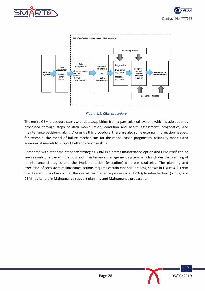
Figure 4.1: CBM procedure
The entire CBM procedure starts with data acquisition from a particular rail system, which is subsequently
processed through steps of data manipulation, condition and health assessment, prognostics, and
maintenance decision-making. Alongside this procedure, there are also some external information needed,
for example, the model of failure mechanisms for the model-based prognostics, reliability models and
economical models to support better decision making.
Compared with other maintenance strategies, CBM is a better maintenance option and CBM itself can be
seen as only one piece in the puzzle of maintenance management system, which includes the planning of
maintenance strategies and the implementation (execution) of those strategies. The planning and
execution of consistent maintenance actions requires certain essential process, shown in Figure 4.2. From
the diagram, it is obvious that the overall maintenance process is a PDCA (plan-do-check-act) circle, and
CBM has its role in Maintenance support planning and Maintenance preparation.

Page 29 05/03/2019
Contract No. 777627
Figure 4.2: General maintenance process (IEC 2004)
4.1 PROPOSED TECHNIQUES TO SUPPORT PREDICTIVE AND PREVENTIVE MAINTENANCE
Technically there are three major tasks in the overall procedure of a CBM system: fault diagnostics,
prognostics, and condition-based maintenance (as shown in Figure 4.3). The first task is to diagnose and
identify the root causes of system failures. The root causes identified can provide useful information for
prognostic models as well as feedback for system design improvement. The second task takes the processed
data and existing system models or failure mode analysis as inputs and employs the developed library of
prognosis algorithms to automatically update degradation models and predict failure times of the system.
The prognostics can be model-based, data-based or a hybrid approach of model and data based. The third
task makes use of the prognosis results (e.g. the distribution of remaining useful life) and considers the cost
versus benefits for different maintenance actions to determine when and how the preventive maintenance
will be conducted to achieve minimal operating costs and risks. Other than these three major tasks, there
are also some other important components listed in Figure 4.3. Nevertheless, they are often prepared
offline and only timely updating may be needed during the system operations. For example, signal
processing/feature extraction is the procedure to pre-process the signals using rules or methods developed
according to engineering knowledge, expert experience, or statistical findings from historical data. They
serve the purpose to eliminate noise, reduce data dimensions (complexities), and transform the data into
proper space for future analysis. Similarly, prognosis and diagnosis algorithms can also be developed offline
to cater the special characters of the signals and system properties. Upon new arrival of sensing signals,
appropriate algorithms can be selected to compute the distribution of remaining useful life (RUL), time to
failure (TTF), probability to failure (POF), determine maintenance actions, or find root causes of
abnormalities.
The reviews on statistical data-driven approaches (Si et al. 2011, Sikorska et al. 2011) have covered most of
the models used in RUL estimation with a statistical orientation. The subsequent sections are devoted to

Page 30 05/03/2019
Contract No. 777627
discussing the techniques which have been applied during the SMaRTE project and some issues related to
the application of the techniques in order to provide some insights for CBM-RS.
Figure 4.3: An illustration of major tasks in a CBM system
4.1.1 DATA PROCESSING AND FEATURE EXTRACTION
Data processing and feature extraction procedures become standard in many complex systems to improve
data quality, reduce data redundancy, and boost efficiency of analysis. Due to its importance, many
researchers have investigated this problem in the literature, as summarized in some of the review papers
in different application areas (e.g. Gaber et al. 2005, Famili et al. 1997, Trier et al. 1996). In this section we
will list some of the commonly used statistical methods in the context of data processing and feature
extraction.
For different data sets, these statistical methods may not be all useful. Meanwhile, it is believed that some
faults will show certain characters in frequency domain. Fourier transform is the most common form of
further signal processing, which decomposes a time waveform into its constituent frequencies. Fast Fourier
transform (FFT) is usually used to generate the frequency spectrum from time series signals. Apart from
these statistical methods, on the other hand, there is another class of methods which utilises some domain
knowledge in the process of feature extractions. Based on the procedure for CBM, these methods could be
summarized into three based on the data types: value type (e.g. temperature, pressure, humidity, etc.),
waveform type (e.g., vibration data), and multidimensional type (e.g. image data, X-ray images, etc.)
(Jardine et al. 2006).
In the SMaRTE project, various methods are applied to identify the thresholds and trending. There is no
golden rule for the feature extraction and once the data is preliminary processed, some features are
obvious, however some are hard to identify. Therefore the visualisation of the data becomes an important
part of feature extraction and is a new challenge when there are multiple sources of data.

Page 31 05/03/2019
Contract No. 777627
Table 5: Commonly statistical method used for time-domain features
Feature Definition
Peak value max = max 𝑛𝑗 (𝑗 = 1,… , 𝑁)
Mean 𝑢 =
1
𝑁 ∑𝑛𝑗
𝑁
𝑗=1
Standard deviation
𝜎 = √1
𝑁 − 1∑(𝑛𝑗 − 𝑢)
2
𝑁
𝑗=1
Root mean square
𝑅𝑀𝑆 = √1
𝑁∑(𝑛𝑗)
2
𝑁
𝑗=1
Skewness 𝑆𝐾 =
∑ (𝑛𝑗 − 𝑢)3𝑁
𝑗=1
(𝑁 − 1)𝜎3
Kurtosis 𝐾𝑈 =
∑ (𝑛𝑗 − 𝑢)4𝑁
𝑗=1
(𝑁 − 1)𝜎4
Crest indicator 𝐶𝐼 =
max |𝑛|
√1𝑁∑ (𝑛𝑗)
2𝑁𝑗=1
Clearance indicator 𝐶𝐿𝐼 =
max |𝑛|
(1𝑁∑ √|𝑛𝑗|𝑁𝑗=1 )2
Shape indicator
𝑆𝐼 = √1𝑁∑ (𝑛𝑗)
2𝑁𝑗=1
1𝑁∑ |𝑛𝑗|𝑁𝑗=1
Impulse indicator 𝑀𝐼 =
max |𝑛|
1𝑁∑ |𝑛𝑗|𝑁𝑗=1
4.1.2 DATA VISULASITION
In theory, to communicate information clearly and efficiently, data visualisation uses statistical
graphics, plots, information graphics and other tools. Numerical data may be encoded using dots, lines, or
bars, to visually communicate a quantitative message. Effective visualization helps users analyse and reason
about data and evidence. It makes complex data more accessible, understandable and usable. Users may
have particular analytical tasks, such as making comparisons or understanding causality, and the design
principle of the graphic (i.e. showing comparisons or showing causality) follows the task. The traditional
methods of data visualisation, for example tables, are generally used where users will look up a specific
measurement, while charts of various types are used to show patterns or relationships in the data for one
or more variables.

Page 32 05/03/2019
Contract No. 777627
Figure 4.4: Examples of data visualisation used in the SMaRTE project
Figure 4.4 shows some examples of data visualisation used in the SMaRTE project: the top plot shows the
occurrence of a particular event for different coaches on a particular fleet (event data), and the bottom
plots shows the correlation matrix of a set of variables (condition data). Overall there are four basic types
of presentation in which a graph can help communication of information efficiently:
Comparison
Composition
Distribution
Relationship
Also, some guidance of how to select a type of graph to present the data is provided in Figure 4.5 below.

Page 33 05/03/2019
Contract No. 777627
Figure 4.5: Selection of a chart type1
4.1.3 DATA DRIVEN PROGNOSTICS METHODS
In the applications of Reliability Centered Maintenance (RCM), one of the strategies for failure
management is on-condition maintenance, also called predictive or condition-based maintenance.
This strategy relies on the capability of detect potential failures in advance in order to take
appropriate actions. The P-F curve, a visual representation of an asset’s deterioration over time, has
become an essential component to any reliability centered maintenance program. The horizontal (X) axis
of the P-F Curve represents time-in-service for an asset, or asset component. The vertical (Y) axis represents
some measure of performance, rate, condition or suitability for purpose. The curve shows that the
performance or condition of an asset or component declines over time from potential failure (P) leading to
functional failure (F), i.e. loss of function for which it was intended. The curve may take various shapes,
linear or exponential, but is generally represented as exponential as shown in Figure 4.6.
1See https://i1.wp.com/www.tatvic.com/blog/wp-content/uploads/2016/12/Pic_2.png?zoom=2&w=450)

Page 34 05/03/2019
Contract No. 777627
The P-F curve conceptually captures the process of system’s degradation, and importantly it explicitly shows
the time range between P and F, commonly called the P-F interval, which is the window of opportunity
during which a imminent failure can be detected and appropriate maintenance actions to address the
failure. In real applications of CBM, it becomes crucial to be able to model the true process of system’s
deterioration over time (or other measurements, for example running distance). In the SMaRTE project, the
aim is to have a hybrid approach of model-based and data-based prognostics. Prognostics algorithms
predict the future reliability of a product considering the collated current and past health information.
Through constant inspection, the observed health information is often referred to as condition data.
Condition data may be directly or indirectly related with the system health status and hence can be viewed
as system health indicators. As a system degrades inevitably through usage, its health status deteriorates
and is manifested through the observed condition data. In practice, failures are often defined as a deviation
of expected performance, thus condition data is normally viewed as the system degradation signal. By
modelling the evolution of degradation and calculating the time it first hits the failure threshold, we will be
able to predict the system RUL, TTF or POF.
Figure 4.6: PF curve in CBM
Due to the typical randomness in the evolution paths of a component/system degradation, the calculated
RUL will be in the form of some probability distribution. Two excellent comprehensive review papers in RUL
research can be found in (Si et al. 2011, Sikorska et al. 2011). In the SMaRTE project, we have also
experienced some techniques, namely hidden Markov models, to model the degradation process as
accurate as possible.
Markov Chain Model - In general, it is assumed that the degradation process {𝑋𝑛, 𝑛 ⩾ 0} evolves
on a finite state space Φ = {0, 1, . . . , 𝑁}, with 0 corresponding to the perfect healthy state and 𝑁
representing the failed state of the monitored system. The RUL at time instant 𝑛 can be defined as
𝑇 = inf { : 𝑋𝑛+𝑡 = 𝑁 | 𝑋𝑛 = ̸𝑁}. The probability transition matrix and the number of the states can

Page 35 05/03/2019
Contract No. 777627
be estimated from historical data. By dividing the health status into discrete states such as “Good,”
“OK,” “Minor defects,” “Maintenance required,” and “Unserviceable,” the method can provide
meaningful results that are easier to be understood by field engineers.
Hidden Markov Model (HMM) - HMM consists of two stochastic processes, a hidden Markov chain
{𝑍 , 𝑛 ⩾ 0}, which is unobservable and represents the real state of the degradation, and an
observable process {𝑌𝑛,𝑛⩾0}, which is the observed signal from monitoring. Similar to
Markovian- based models, it is assumed that the degradation process evolves according to a
Markov chain on a finite state space. Generally, a conditional probability measure (𝑌𝑛 | 𝑍𝑛 = 𝑖),
𝑖∈Φ, is used to link {𝑌𝑛,𝑛⩾0}and{𝑍𝑛,𝑛⩾0}. As such the RUL at time instant 𝑛 can be defined as 𝑇 =
inf { : 𝑍𝑛+𝑡 = 𝑁|𝑍𝑛 =�̸�,𝑌𝑗,0≤𝑗≤𝑛}.The model is preferred when only indirect observations are
available (Ghasemi 2010).
4.2 CRITICAL CHALLENGES FOR CBM-RS
The definition of CBM implies there are three critical challenges for CBM to be successful. The first critical
challenge is the determination of system health indicator. CBM requires that there is some means of
determining the parameter (or parameters) to reflect the true condition of the system. For some simple
systems (i.e. either the architecture of system is simple enough or the failure mechanism is well studied), it
is easy to determine which parameter is the most adequate choice for the condition monitoring. However,
some new or complex systems, especially when a system consists of both mechanical and electronical
components, for example a traction control unit, it is difficult to select the right parameter(s). In the SMaRTE
project, we have attempted to establish a CBM system for a particular model of traction control unit. In this
example there are total of 195 parameters (of which some are listed in Table 3) and after experimenting
with a number of different techniques for selecting the right system health indicators, it was concluded that
the principle component analysis (PCA) is one of the most powerful techniques for this system.
PCA is a type of linear transformation on a given data set that has values for a range of variables
(coordinates) for a certain amount of spaces. This linear transformation fits this dataset to a new coordinate
system in such a way that the most significant variance is found on the first coordinate, and each
subsequent coordinate is orthogonal to the last and has a lesser variance. In this way, you can transform a
set of x correlated variables over y samples to a set of p uncorrelated principal components over the same
samples. In simple words, PCA is a method of extracting important variables (in form of components) from
a large set of variables available in a data set. It extracts low dimensional set of features from a high
dimensional data set with a motive to capture as much information as possible. With fewer
variables, visualization also becomes much more meaningful. PCA is more useful when dealing with 3 or
higher dimensional data. It is always performed on a symmetric correlation or covariance matrix. This
means the matrix should be numeric and have standardized data.

Page 36 05/03/2019
Contract No. 777627
Figure 4.7:1 Examples of PCA in the project
Figure 4.7 shows some examples of PCA undertaken in the project. Among the 195 variables, there are 5
groups, overall control variables, T1M1 (Traction Unit 1 Module 1), T1M2, T2M1, and T2M2. The left
diagram in Figure 4.7:1 shows the PCA of several variables which are parameters of T1M1; and the right
diagram is a plot of PCA on all variables of T1M1.
The second critical challenge is the accuracy and interval of condition monitoring. CBM requires that there
is some means of determining the true condition of the system. This is usually done by inspection or sensing.
The accuracy and frequency of inspection or data sensing will directly affect the result of CBM. In the
SMaRTE project, we have explored several prediction techniques, including Least Mean-Square (LMS)
algorithm, Hidden Markov Model (HMM), and Time Delay Neural Network (TDNN), to obtain an accurate
enough health curve (PF curve) for prediction.
Least-mean-squares (LMS) algorithms are a class of adaptive filter used to mimic a desired filter by
finding the filter coefficients that relate to producing the least mean square of the error signal
(difference between the desired and the actual signal). It is a stochastic gradient descent method
in that the filter is only adapted based on the error at the current time.
Figure 4.8: LMS prediction model

Page 37 05/03/2019
Contract No. 777627
Time delay neural network (TDNN) is a multilayer artificial neural network architecture whose
purpose is to 1) classify patterns with shift-invariance, and 2) model context at each layer of the
network. Shift-invariant classification means that the classifier does not require explicit
segmentation prior to classification. For the classification of a temporal pattern (such as speech),
the TDNN thus avoids having to determine the beginning and end points of sounds before
classifying them. For contextual modelling in a TDNN, each neural unit at each layer receives input
not only from activations/features at the layer below, but from a pattern of unit output and its
context. For time signals each unit receives as input the activation patterns over time from units
below. Applied to two-dimensional classification (images, time-frequency patterns), the TDNN can
be trained with shift-invariance in the coordinate space and avoids precise segmentation in the
coordinate space.
Figure 4.9: TDNN architecture
The experiment of TDNN within SMaRTE evaluated the conclusions in various reviews of TDNN (Waibel et
al. 1989, Narendra et al 1990) that the effectiveness of TDNNs in processing wider context inputs was shown
in small and large data scenarios. Further using efficient selection of sub-sampling indices speed-ups were
be obtained during training.
The research presented in this report is only a preliminary investigation into these techniques, however it
can conclude that the prediction models for different event codes are different. The adaptive filter
technique (LMS) and artificial intelligence approach (TDNN) are all usable in some sense, and may not be
working on some other data set (i.e. less accurate).
The last critical challenge is the determination of condition limits. The condition limit has a direct effect on
the life of the system and the operation cost of the system. Before the system is put into the service, it has
a static (pre-defined) condition limit, but this limit can change during the operation time due to various

Page 38 05/03/2019
Contract No. 777627
operation modes and environment. It is essential to know the in-service condition limits. During the SMaRTE
project, we explored various options to determine the in-service condition limits. Figure 4.10 shows the
analysis of failure rates. It clearly shows that there is an obvious jump of the occurrence rate after the train
travels 8 × 10⁵ 𝑘𝑚.
Figure 4.10: Occurrence of a certain event over the distance
4.3 SUMMARY
Condition Based Maintenance (CBM) can be defined as maintenance actions based on the real-time
operational state obtained from tests, operation and condition measurements (Mitchell, 1998). According
to this definition maintenance actions should be based on the actual condition, with an objective evidence
of need, to be executed only at a specific time as to not to suffer a breakdown or a malfunction. The
knowledge of the real-time operational state can be assessed using different degree of automation, from
human visual inspections to fully automated systems. CBM is a strategy or policy which guides maintenance
works has been undertaken.
The foundation of a CBM system is its data processing procedure. Through constant inspection or
monitoring, the observed health information is often referred to as condition monitoring (CM) data. CM
data may be directly or indirectly related with the system health status and hence can be viewed as system
health indicators. In current data rich environment, huge amounts of data are often automatically collected
in a short time period. The overwhelming data poses new challenges to the interoperability in data
management, analysis, and interpretation.
In this report, we introduced the model and requirements of data in a CBM system. We introduced some
techniques and methods explored during Tasks 2.2 and 2.3 of the project which will be investigated in more
details through application to a range of case studies in Task 2.4 and reported in Deliverable D2.3.

Page 39 05/03/2019
Contract No. 777627
5. OPTIMISATION OF MAINTENANCE DECISIONS
This chapter explores tools and quantitative techniques to support and optimize maintenance decisions.
Section 5.1 explores techniques to support maintenance decisions, in specific a Markov Decision Process
(MDP) approach is explored. Section 5.2 presents a prototype of a rolling stock management system: i) a
model on tactical maintenance planning (in subsection 5.2.1) and ii) a model on operational maintenance
scheduling (in subsection 5.2.2).
5.1 ANALYSIS TECHNIQUES TO SUPPORT MAINTENANCE DECISIONS
This section explores the analysis techniques that support maintenance decisions from a life-cycle
perspective. The mathematical problem of predicting and optimizing maintenance decisions is formulated
following a Markov Decision Process (MDP) approach with the main aim to derive an optimal decision map
depending on the condition of the component under analysis.
The decision problem of maintaining a rolling stock component is then formulated as a Markov Decision
Process (MDP), with the aim to provide a way to support Condition-Based Maintenance (CBM) for that
component. A practical example is also provided to illustrate the use of this technique to derive a CBM
optimal strategy for a wheelset railway component.
A Markov Decision Process is a model for sequential decision making under uncertainty, which takes into
account both the outcomes of current decisions and future decision-making opportunities
(Puterman 2005). From a practical point of view, its key ingredients are:
i) a set of decision epochs or periods – 𝑡 ∈ {1, 2, … , 𝑇};
ii) a set of system states – 𝑠 ∈ {𝑠1, 𝑠2, … , 𝑠𝑁};
iii) a set of available actions – 𝑎 ∈ {𝑎1, 𝑎2, … , 𝑎𝑀};
iv) a set of state and action dependent immediate rewards or costs – 𝑞(𝑠, 𝑎);
v) a set of state and action dependent transition probabilities – 𝑝(𝑠′| 𝑠, 𝑎).
Markov chains are specific mathematical models in stochastic processes that describe the evolution of a
system (or component) that passes successively through different states and are commonly used to
represent random paths in networks or graphs, and to predict the long-term behaviour of the
process/system (Sheskin 2016). In fact, when larger horizons of analysis are required, Markov Chains tend
to be a better modelling choice compared to other state-of-the-art techniques for stochastic processes
(Pathak et al. 2015).
A Markov stochastic process will respect the Markov property for stationary transition probabilities, which
states that the probability of the next state, conditioned on all history, depends only on (the probability of)
current state, and not on all the past history of states visited before by the system. In stationary or
homogeneous Markov processes, where the transition probabilities are independent of the period at which
the transition occurs, the Markov property can be written as follows:

Page 40 05/03/2019
Contract No. 777627
𝑃 (𝑋𝑛+1 = 𝑖𝑛+1 | 𝑋𝑛 = 𝑖𝑛, 𝑋𝑛−1 = 𝑖𝑛−1, … , 𝑋0 = 𝑖0) = 𝑃 (𝑋𝑛+1 = 𝑖𝑛+1 | 𝑋𝑛 = 𝑖𝑛)
Note that the equation above is an equality between two conditional probabilities, and the conditional
probabilities are usually called transition probabilities and the transition matrix at epoch or period 𝑛 is
denoted as 𝑃(𝑛) ≡ [𝑝𝑖,𝑗,(𝑛)] ≡ 𝑃(𝑋𝑛+1 = 𝑗 | 𝑋𝑛 = 𝑖) , whose entries are the probabilities that the
system/component moves to state 𝑗 in epoch 𝑛 + 1, given that in epoch 𝑛, the system was in state 𝑖, (with
𝑖, 𝑗 ∈ {1, 2, … , 𝑆}).
At any given epoch 𝑛, the transitions between states can be depicted in an oriented network node graph
as presented in Figure 5.1 and their probability values represented in a transition matrix, also called Markov
Transition Matrix (MTM):
SSSSS
S
S
S
ji
pppp
pppp
pppp
pppp
pP
,3,2,1,
,33,32,31,3
,23,22,21,2
,13,12,11,1
,
Figure 5.1: Transitions between states and corresponding transition probabilities
Note that a Markov Matrix has all non-negative inputs and its values are all 0 ≤ 𝑝𝑖,𝑗 ≤ 1. Moreover, it is
easily shown that a transition from one state to any other state (including staying at the same one) is a
certain event, i.e. the sum of all entries for a given row 𝑖 in transition matrix 𝑃 ≡ [𝑝𝑖,𝑗] is equal to one
(∑ 𝑝𝑖,𝑗 = 1𝑆𝑗=1 ).
Moreover, let 𝑋𝑛 be a row vector (whose entries are the probabilities that the process is at epoch 𝑛 for
each possible state), then at the next epoch 𝑛 + 1, the process can evolve to different states and the row

Page 41 05/03/2019
Contract No. 777627
vector 𝑋𝑛+1, whose entries are the probabilities that the process is at epoch 𝑛 + 1 for each possible state,
is obtained by computing 𝑋𝑛+1 = 𝑋𝑛 ∙ 𝑃(𝑛) (which only depends on the 𝑋𝑛 immediately before and the
transition matrix 𝑃(𝑛) ). As very often it is assumed that the transition matrix is stationary (remaining
constant for every epoch, i.e. 𝑃(𝑛) = 𝑃), then the succession of {𝑋𝑛} can be obtained as follows:
𝑋0
𝑋1 = 𝑋0 ∙ 𝑃(0) = 𝑋0 ∙ 𝑃
𝑋2 = 𝑋1 ∙ 𝑃(1) = (𝑋0 ∙ 𝑃) 𝑃 = 𝑋0 ∙ (𝑃𝑃) = 𝑋0 ∙ 𝑃
2
𝑋3 = 𝑋2 ∙ 𝑃(2) = (𝑋0 ∙ 𝑃
2) 𝑃 = 𝑋0 ∙ (𝑃2𝑃) = 𝑋0 ∙ 𝑃
3
⋯
𝑋𝑛 = 𝑋0 ∙ 𝑃𝑛
This result allows the computation of probabilities to future states in a Markov process if the transition
matrix of the process is known and the row vector at epoch 𝑛. Let k, k ∈ {0, 1, 2, … }, be the number of
periods that have passed from the epoch 𝑛 , the probabilities of visiting any state is computed as
𝑋𝑛+𝑘 = 𝑋𝑛𝑃𝑘 . This ease of access and computation of the probabilities of visiting future states and
flexibility are the major advantages of Markov Models.
Then, a Markov Decision Process (MDP) is a controlled stochastic process in which a decision-maker is
uncertain about the exact effect of executing a certain action, in the sense that, the system may transit to
another state with a certain probability and visiting that state has a certain cost or reward
(Papakonstantinou and Shinozuka 2014). The goal is then to optimize the intended objective function (e.g.
maximize the sum of all rewards or an average reward, or alternatively minimize the sum of all costs or
average cost), over the set of solutions that are feasible for each state, supporting the decision-maker to
take the best action at certain times/epochs in the timeline, and then preventing or limiting the
deterioration of the objective (Gabrel et al. 2014). The set of actions that should be taken (usually
depending on the state that the system is) is called a policy (Papakonstantinou and Shinozuka 2014). In this
way, for any time step (𝑡), where the system is in a certain state (𝑠) and the agent takes an action (𝑎) of a
finite set of actions, an MDP will provide a specific corresponding reward (or cost) as a result of the chosen
action. Each time the system visits state 𝑖 at epoch 𝑛, a reward is earned.
The reward vector (𝑞𝑖 ∈ ℝ𝑟) is assumed to be stationary over time, similar to what happened with the
transition probability (𝑝𝑖,𝑗 ), and the reward vector represents the immediate independent rewards
associated to the value of each process’ state. Using probability theory, the scalar expected value for the
total reward received after 𝑛 epochs can be computed as 𝐸[𝑅(𝑛)] ≡ �̅�(𝑛) = 𝑋0𝑃𝑛𝑞𝑖 = 𝑋𝑛𝑞𝑖.
The MDP is a sequential decision process for which the decisions produce a sequence of Markov Chains
with Rewards (MCR). If decisions have to be taken to change, in our benefit, the natural path of the
evolution of the Markov chains, there must be a series of possible actions allied to the process, for each
action 𝑘 there is a corresponding reward vector 𝑞𝑖𝑘 that will generate a different MCR. The set of best

Page 42 05/03/2019
Contract No. 777627
actions to take for each of the possible states is called an optimal policy according to a given criterion (or
an optimal decision map). This rule is considered stationary over an infinite planning horizon, which means
that the optimal policy will always specify the same decision in a given state, and works together with the
blocks of MCRs. The computational procedure that is most used to solve an MDP problem over an infinite
planning horizon is linear programming. There are other computational procedures such as: exhaustive
enumeration, value iteration and policy iteration.
Exhaustive enumeration is computationally prohibitive unless the problem is extremely small. Value
iteration requires less arithmetic operations than these alternative procedures, though it may never satisfy
a given stopping condition. Policy iteration maximizes the gain or the average gain/reward per period.
Finally, linear programming is formulated with the support of computer software packages, which are
capable of solving both linear problems. Due to the complexity of the process, for multi-state chains, linear
programming is imperative.
Since in condition-based maintenance, we are dealing with economic values and balances, the last
parameter to be considered for the MDPs is the discount factor, 𝛾 ∈ [0, 1], which represents the difference
in importance between future rewards and present rewards, it can be related with a discount rate (𝑟), as
𝛾 =1
1+𝑟, and thus, it is used to obtain the expected present values.
This new factor will also take part in the calculus of the expected total values, being now the expected total
discounted value rewards. The calculus of these values are iterative processes used in the linear
programming for solving MDPs. For a finite horizon, being 𝑇 the number of periods and 𝑣𝑖(𝑛 + 1) the
vector representing the expected maximum total rewards of the next epoch 𝑛 + 1 , the vector 𝑣𝑖(𝑛)
represents the expected maximum total rewards earned from epoch 𝑛 to 𝑇 when in state 𝑖 at epoch 𝑛
considering all the actions:
𝑣𝑖(𝑛) = max𝑘[𝑞𝑖𝑘 + 𝛾∑𝑝𝑖,𝑗
𝑘 𝑣𝑖(𝑛 + 1)
𝑆
𝑗=1
]
for 𝑛 = 0, 1,⋯ , 𝑇 − 1.
Having presented the MDP framework that is followed as part of an analysis technique to support
maintenance decisions, an illustrative example focused on a railway wheelset is explored here.
5.1.1 ILLUSTRATIVE EXAMPLE ON RAILWAY WHEELSET COMPONENT
The railway wheelset is one of the most important components of modern train systems, since it allows the
train to curve, keep it on track, while ensuring the passenger comfort and avoiding train derailment.
However, it is also one of the top three train components most affected by wear and damage. This causes
serious implications for the passenger safety and comfort, as well as for the wheelset life-cycle itself.
Therefore, to avoid performance degradation, wheelsets need to go through rigorous inspections and

Page 43 05/03/2019
Contract No. 777627
maintenance processes to ensure a high quality level to the railway service. As wheelsets change its shape
due to wear and damage, a comprehensive model that can predict its shape evolution and damage
occurrence, throughout its life cycle, is needed.
There are three geometric variables (as shown in Figure 5.2), measured from a tread datum position point
(T) and a point A, which are indicators that are monitored in the evolution of the wheelset degradation: i)
the wheel diameter (𝐷), ii) the flange height (𝐹ℎ) and the flange thickness (𝐹𝑡). Apart from the changes in
shape, it can also occur damages in the rolling surface. The most common types of damage detected are:
rolling contact fatigue (RCF), cavities and wheel flats.
Figure 5.2: Transitions between states and corresponding transition probabilities
As wheelsets take a critical role concerning the motion of the vehicles and the passenger comfort, their
dimensions must comply with tight standards for the wheel shape and diameter. On the other hand, due
to their use and mileage, wheel profiles will wear and damage will eventually occur, and thus, inspection
activities should monitor and control the evolution of the main indicators of degradation, and restore them
if damage occurs and/or wear is higher than certain limits.
The restoration of the shape of a wheelset can be scheduled within a preventive maintenance plan -
planned actions - or in the corrective maintenance actions - remedial actions. However, the maintenance
actions incur in material waste and higher maintenance costs, and thus an optimized maintenance strategy
is needed that could predict the wear evolution and choose the more efficient maintenance actions for
each wheelset wear/damage situation.
Concerning the train wheel maintenance process, after an inspection activity is conducted, two
corrective/preventive maintenance situations are possible:
The wheel is re-profiled (either on corrective or preventive maintenance);
The wheel is replaced by a new one.

Page 44 05/03/2019
Contract No. 777627
To define the state space, three main indicators were used: the diameter change, the occurrence of damage
and the mileage since last turning. A total of 1620 states were defined, according to the previous indicators
and a set of three actions were defined: i) “do nothing”, ii) “renewal” and iii) “turning”. Markov Transition
Matrices (MTM) for each action and values for the reward/cost function were both estimated. Finally, the
optimal policy was derived, leading to a optimal decision map, which can support the decision-maker to
take the best maintenance choice for each wheelset state.
Figure 5.3 shows an example of the possible transitions if renewal action is chosen. Note that for each state,
the only possible transition is from that state to the initial one (without damage and initial diameter, i.e. as
new).
Figure 5.3: Example of transition probabilities for “renewal” action from states with and without damage to the initial state (initial Diameter and without damage).
Figure 5.4 shows the resulting optimal decision map that specifies the best action depending on the
condition/state that the wheelset is. Note that each small square represents a state defined by mileage (or
kilometres) since last turning (from 0 to 250 thousand miles) and the diameter (from the initial diameter
850 mm to the scrap diameter 790 mm).
Figure 5.4 shows that, for the MTM assumed, preventive maintenance actions (preventive turning) would
be advisable for railway wheelsets with a mileage since last turning between 210 and 240 thousand miles
and a wheel diameter between 799 and 801 mm. In the remaining cases, it is advisable that the wheelset
should run until the 250 thousand miles (if not damage occurs), be turned if a damage has occurred.
This illustrative example will be explored in further detail (in D2.3 on the case studies) with real data from
the train operating companies involved in this project.

Page 45 05/03/2019
Contract No. 777627
Figure 5.4: Example of an optimal decision map for each state
5.2 PROTOTYPE OF ROLLING STOCK MANAGEMENT SYSTEM
A prototype of rolling stock management system is explored in this section, namely with the
integration of a tactical maintenance planning model (in subsection 5.2.1) and an operational
maintenance scheduling model (in subsection 5.2.2). Maintenance Management systems for rolling
stock must take into account technical and operational constraints in order to plan and schedule
maintenance actions in a given time window. Moreover, maintenance of a large fleet in train operating
companies requires careful planning and efficient management of resources. Therefore, Integer Linear
Programming (ILP) models are developed for the tactical planning model and for the operational
maintenance scheduling model.

Page 46 05/03/2019
Contract No. 777627
5.2.1 RELATED PAST WORK
Optimization models for preventive maintenance actions in transportation companies have been proposed
for buses (Haghani and Shafani 2002), air transport (Bazargan 2015) and rail transport (Maróti and Kroon
2007, Doganay and Bohlin 2010, Bohlin and Wärja 2015, Lai et al. 2017). Moreover, there is also an
extensive literature on integrating maintenance planning in rolling stock operations in a network (Mároti
and Kroon 2004, Mároti and Kroon 2005, Budai et al. 2006, Caprara et al. 2006, Giacco et al. 2014, Santos
et al. 2015).
Haghani and Shafahi (2002) studied a way to perform maintenance of buses mostly during their idle time
in order to reduce the number of maintenance hours for vehicles that are pulled out of service. The solution
of the optimization model is a maintenance schedule for each bus due for inspection as well as the minimum
number of maintenance lines that should be allocated for each type of inspection over the scheduled period.
Bazargan (2015) studied how to minimize the cost of maintenance and maximize aircraft availability and
then compared with several possible planning: closest to maintenance (the aircraft closest to its scheduled
maintenance is dispatched); furthest to maintenance (the aircraft farthest to its next scheduled
maintenance is dispatched); random maintenance (selects randomly an aircraft for maintenance); cheapest
next maintenance (the aircraft with the cheapest upcoming maintenance is dispatched); equal aircraft
utilization (the aircraft with lowest utilization is dispatched).
Maróti and Kroon (2004, 2005, 2007) made an important contribution in the topic of maintenance routing.
They started with the definition of ‘a scenario model’ (Maróti and Kroon 2004) and later on extended it
with ‘a transition model’ (Maróti and Kroon 2005) and with ‘an interchange model’ (Maróti and Kroon 2007).
The ‘scenario model’ (Maróti and Kroon 2004) followed a flow-type model in graph representation of a
railway network and it aimed to select a collection of pairwise independent changes, so that the urgent
train units are routed to a node representing a maintenance task. The ‘transition model’ (Maróti and Kroon
2005) only incorporates information on transitions that are allowed (i.e. there is enough time to carry out
shunting operations without causing delays to normal train schedules. Later on, Maróti and Kroon (2007)
put forward ‘an interchange model’, which explored a way to allocate a train (to a maintenance yard far
from its current location) to daily service. The objective was to maximize the number of journeys with
passengers on board, on its route to the maintenance yard, and thus reducing the number of journeys in
which the train is empty. Therefore, if the train travels a long distance as an empty train to perform a
maintenance activity, it would significantly increase the overall generalized cost of that maintenance
activity. In order to solve this problem, the authors propose an interchange model that checks the feasibility
of all possible changes and provide an interactive decision support system that proposes candidate
interchanges to maintenance routing planners. Lai, Wang, and Huang (2017) automated the planning
process and according to their results, improved the efficiency of rolling stock usage by 3% up to 4% when
compared with the plans elaborated by experienced railway practitioners. Their objective function is to
minimize the gap between the current mileage of the train set and the upper limit each day in order to find
the best planning possible. They considered that the ‘best’ solution is the one that maximizes the utilization

Page 47 05/03/2019
Contract No. 777627
rate of rolling stock and minimizes/eliminates non-revenues operations, while allocating the maintenance
activities in the planning horizon.
Maintenance planning has been studied by Doganay and Bohlin (2010) and their model was later expanded
in Bohlin and Wärja (2015). First model was built specifically for a train fleet, whereas the second model is
more general in nature and can be adapted to other industries like the oil industry. Both models attempt
to minimize the total maintenance costs, including the costs of keeping spare parts (inventory costs). These
two works are the ones more related to the present ILP tactical maintenance model, with additional
constraints regarding the maintenance yard configuration and lines.
Moreover, in rail transport planning literature, some models deal with the rolling stock planning using an
integrated approach (Thorlacius et al. 2015, Tréfond et al. 2017), while include the maintenance
requirements as technical constraints, which mainly require that each train unit goes to the depot a
prescribed number of times during that period and it stays in the depot for a certain amount of time so that
maintenance occurs. Other models balance track possession for infrastructure maintenance and train
operation schedules (Forsgren et al. 2013, Lidén and Joborn 2016).
An overview of the state-of-the-art on operations research models and techniques used by passenger
railway operators (Huisman et al. 2005) classifies planning problems by its planning horizon, showing that
they can be divided in three planning phases: strategic, tactical and operational. Operational planning
handles with the details of the timetable, namely the rolling-stock and crew schedules. The rolling-stock
circulation problem allocates rolling-stock units to the trips. Routing of rolling-stock may include the
maintenance visits to maintenance facilities/depots, and thus, such maintenance visits of train units may
already be incorporated in the rolling stock circulation problem, with typical constraints of each unit
spending at least a certain amount of time in the depot during the planning period. Note that such
constraints do not incorporate all the information associated with maintenance actions. However,
maintenance scheduling in the rolling stock problem is often ignored and integrated models that
simultaneously schedule maintenance tasks and railway operations are scarce in the literature. A
robustness perspective on the rolling-stock planning problem has been adopted by Tréfond et al. (2017) for
the French passenger trains. Such concept of robustness is discussed using some indicators to assess the
rolling-stock rosters, aiming to homogenize turning-times, and absorb potential delays. In their work,
Tréfond et al. (2017) use an ILP model to find a robust solution in the rolling-stock planning problem,
observing a significant improvement in robustness indicators while maintaining low operating costs and
meeting maintenance requirements. However, their maintenance approach simply considers a
maintenance period in which all train units must benefit from maintenance at least once every three days,
introducing maintenance slots in their schedule.
Rescheduling approaches have also been discussed using integer programming models to solve the
timetable rescheduling problem by minimizing the number of cancelled and delayed trains while adhering
to infrastructure and rolling stock capacity constraints. Cacchiani et al. (2014) provides an overview of
recovery models and algorithms for real-time railway scheduling. Binder et al. (2017) also explored the
timetable rescheduling problem but from a multi-objective perspective. Cordeau et al. (2001) put forward

Page 48 05/03/2019
Contract No. 777627
an optimization model to assign locomotives and cars to passenger trains, while complying with
maintenance requirements. Giacco et al. (2014) also looked at the rolling stock rostering optimization
problem using under maintenance constraints.
Luan et al. (2017) have recently proposed an integrated optimization model for train scheduling
incorporating maintenance time slots planning. In (Luan et al. 2017) a Lagrangian relaxation approach for
solving the model was pursued and tested on a realistic network adapted from a Chinese railway network.
5.2.2 TACTICAL MAINTENANCE PLANNING
Train operating companies have to plan their maintenance in advance, so that maintenance tasks are
conducted in non-operating hours, i.e. without causing perturbation in the normal service or operation.
These maintenance tasks are performed in a maintenance yard or depot with different maintenance lines
or depot tracks. The allocation of these maintenance tasks in the different maintenance lines in a
maintenance depot is an important task in the maintenance planning. Some maintenance tasks can only be
performed in specific maintenance lines.
This tactical maintenance planning model discusses how to plan maintenance actions in train operating
companies in an annual plan with a time step of a week, while ensuring that several constraints are
complied. An Integer Linear Programming (ILP) model is put forward to plan maintenance in train operating
companies, in which the main aim is to schedule preventive maintenance activities for a train fleet.
DEFINITION OF ILP TACTICAL MAINTENANCE PLANNING MODEL
Let us describe the ILP model, namely: i) the indices, ii) sets, iii) parameters, iv) decision variables and v) the
objective function which is subject to several constraints.
The problem is to build a maintenance plan that covers all train units and maintenance activities scheduled
at given times and maintenance line, and the number of spare parts needed. Spare parts are vehicle parts
which are available so that they can be replaced and repaired without affecting the normal operation of
the service. The goal of the ILP model is to create a tactical maintenance plan that minimizes a cost function,
which respects the periodicity of maintenance actions, and maintenance yard constraints associated for
instance with human resources. Maintenance planners have to know when each train unit will benefit from
preventive maintenance activities. For that purpose, a maintenance planning is required, which provides
the scheduling of all maintenance activities at different time units (e.g. every week) in a planning horizon
(e.g. a year).
In the following formulation, a train unit is defined as a group of vehicles connected with each other and
each vehicle has typically two bogies and four wheelsets (two per bogie).

Page 49 05/03/2019
Contract No. 777627
i. Indices
𝑢 train unit 𝑡 time unit 𝑖 maintenance activity type 𝑝 spare part type 𝑙 maintenance line (or maintenance depot track)
ii. Sets
𝑈 set of train units u 𝐼 set of maintenance activities i 𝑇 set of time units t 𝑃 set of spare parts p 𝐿(𝑖) set of available maintenance lines l in the maintenance yard for maintenance activity i
iii. Parameters
𝐶(𝑖) cost of maintenance activity i 𝑇(𝑖) period of maintenance activity i (in time unit) 𝑓(𝑖) amount of work required to perform maintenance activity i (in person-hour) 𝑑(𝑖) duration of the maintenance activity i. (This is calculated as the ratio between the
amount of work fi and the number of people performing the maintenance activity i) 𝑃(𝑝) cost of having a spare part p per time unit t 𝑞(𝑖, 𝑝) number of spare parts of type p needed to perform maintenance activity i 𝑅(𝑝) duration of the maintenance of spare part p (in time unit) 𝐴(𝑝) maximum amount of spare parts of type p 𝑂(𝑢, 𝑖) time interval since last maintenance activity i for train unit u and the beginning of the
planning horizon
𝐻 planning horizon 𝑆 shunting cost 𝑘 maximum working load per time unit t (in person-hours) 𝑤 maximum working time per time unit t (in hours) 𝑁 number of maintenance activities I (Note: it is the cardinality of the set I) 𝑒 amount of time needed to move a train from a maintenance line l (in hours) 𝑢1 maximum number of train units available 𝑢2 number of train units needed to perform daily service
Parameter 𝑘 is a scalar and is calculated as the product of three quantities: i) number of personnel, ii) the
maintenance duration per day and iii) the number of working days per time unit t. Moreover, scalar 𝑤 is
calculated as the product of two quantities: i) maintenance duration per day and ii) the number of working
days per time unit t.

Page 50 05/03/2019
Contract No. 777627
iv. Decision variables
𝑥(𝑢, 𝑖, 𝑡, 𝑙) binary variable set to 1 if maintenance activity i is performed on train unit u at t time unit, and set to 0 otherwise.
𝑦(𝑢, 𝑡) binary variable set to 1 if unit u is under maintenance at t time unit, and set to 0 otherwise.
𝑈(𝑝) non-negative integer variable corresponding to the minimum amount of spare
parts required to perform the maintenance planning
v. Objective Function
min∑∑∑ ∑ C(i)
𝑙 ∈𝐿(𝑖)𝑡 ∈𝑇𝑖 ∈𝐼
∗ 𝑥(𝑢, 𝑖, 𝑡, 𝑙)
𝑢∈𝑈
⏞ 𝐴
+ ∑ ∑𝑆 ∗ 𝑦(𝑢, 𝑡)
𝑡 ∈𝑇𝑢 ∈𝑈
⏞ 𝐵
+ 𝐻 ∗ ∑ P(p) ∗ 𝑈(𝑝)
𝑝 ∈ 𝑃
⏞ 𝐶
+1
(𝑢1 − 𝑢2) ∗ 𝑁 ∗ 𝐻 ∑∑∑ ∑ (𝐻 − 𝑡) ∗ 𝑥(𝑢, 𝑖, 𝑡, 𝑙)
𝑙 ∈𝐿(𝑖)𝑡 ∈𝑇𝑖 ∈𝐼𝑢∈𝑈⏟ 𝐷
Subject to:
∑ ∑ 𝑥(𝑢, 𝑖, 𝑡, 𝑙)
𝑙 ∈𝐿(𝑖)
≥ 1
𝑡+𝑇(𝑖)
𝑗=𝑡
∀ 𝑢 ∈ 𝑈, 𝑖 ∈ 𝐼, 𝑡 ∈ {1,… ,𝐻 − 𝑇(𝑖) + 1} (2)
∑ ∑ 𝑥(𝑢, 𝑖, 𝑡, 𝑙)
𝑙 ∈𝐿(𝑖)
≥ 1 ∀ 𝑢 ∈ 𝑈, 𝑖 ∈ 𝐼 𝑠𝑢𝑐ℎ 𝑡ℎ𝑎𝑡 𝑇(𝑖) − 𝑂(𝑢, 𝑖) ≤ 𝐻
𝑇(𝑖)−𝑂(𝑢,𝑖)
𝑗=1
(3)
𝑦(𝑢, 𝑡) ≥ 𝑥(𝑢, 𝑖, 𝑡, 𝑙) ∀ 𝑢 ∈ 𝑈, 𝑖 ∈ 𝐼, 𝑡 ∈ 𝑇, 𝑙 𝑖𝑛 𝐿(𝑖) (4)
∑∑ ∑ ∑ 𝑞(𝑖, 𝑝) ∗ 𝑥(𝑢, 𝑖, 𝑡, 𝑙) ≤ 𝑈(𝑝) ∀ 𝑝 ∈ 𝑃, 𝑡 ∈ {1,… ,𝐻 − 𝑅(𝑝)}
𝑡+𝑅(𝑝)
𝑗=𝑡𝑙 ∈𝐿(𝑖)𝑖∈𝐼𝑢∈𝑈
(5)
𝑈(𝑝) ≤ 𝐴(𝑝) ∀ 𝑝 ∈ 𝑃 (6)
∑∑𝑓(𝑖) ∗ 𝑥(𝑢, 𝑖, 𝑡, 𝑙)
𝑖∈𝐼
≤ 𝑘
𝑢∈𝑈
∀ 𝑡 ∈ 𝑇, 𝑙 ∈ 𝐿(𝑖) (7)
∑∑𝑑(𝑖) ∗ 𝑥(𝑢, 𝑖, 𝑡, 𝑙)
𝑖 ∈ 𝐼𝑢∈𝑈
+ 𝑒 ∗ [(∑∑𝑥(𝑢, 𝑖, 𝑡, 𝑙)
𝑖 ∈ 𝐼𝑢∈𝑈
) − 1] ≤ w ∀ 𝑡 ∈ 𝑇, 𝑙 𝑖𝑛 𝐿(𝑖) (8)
∑ 𝑥(𝑢, 𝑖, 𝑡, 𝑙)𝑙 𝑖𝑛 𝐿(𝑖)
≤ 1 ∀ 𝑢 ∈ 𝑈, ∀ 𝑖 ∈ 𝐼, ∀ 𝑡 ∈ 𝑇 (9)

Page 51 05/03/2019
Contract No. 777627
𝑥(𝑢, 𝑖, 𝑡, 𝑙) ∈ {0,1} ∀ 𝑢 ∈ 𝑈, 𝑖 ∈ 𝐼, 𝑡 ∈ 𝑇, 𝑙 𝑖𝑛 𝐿(𝑖) (10)
𝑦(𝑢, 𝑡) ∈ {0,1} ∀ 𝑢 ∈ 𝑈, 𝑡 ∈ 𝑇 (11)
𝑈(𝑝) ∈ ℕ+ ∀ 𝑢 ∈ 𝑈, 𝑡 ∈ 𝑇 (12)
The objective function is the total cost of preventive maintenance over a year and it was adapted from the
objective function in Doganay and Bohlin (2010), which minimizes all maintenance costs of trains in a
railway maintenance yard. This function is composed of four different cost components which are the
maintenance cost component (denoted A); the shunting cost component (denoted B); the spare parts cost
component (denoted C) and finally a cost component to avoid early maintenance (denoted D). The objective
function is then A+B+C+D.
The maintenance cost A is the cost of doing every maintenance activity over the planning horizon, and 𝐶(𝑖)
is the cost of maintenance activity i. The cost component A can then be expressed as the sum of the
maintenance costs of all the maintenance activities for every trains, every line and at every time period
until the planning horizon.
The cost component B is the shunting cost; it corresponds to the cost of pulling a train out of its regular
duty in order to perform maintenance on this train. It can be expressed as the sum of the shunting cost per
time unit 𝑡 of all trains stopped every time period until the planning horizon.
The cost component C represents the cost for storing spare parts. Each spare part cost 𝑃(𝑝) is an input (i.e.
a parameter of the model), and it is estimated as a percentage of the acquisition cost of the spare part 𝑝
(Doganay and Bohlin 2010, Bohlin and Wärja 2015). The cost component C is the product of the duration in
time units of the planning horizon and the sum of the spare part cost times the amount of each spare part.
In the proposed model, the minimum amount of spare parts required remains the same throughout the
planning horizon, as it is assumed that maintenance planners need to know at the beginning of the plan
how many spare parts they will need to acquire. Therefore, 𝑈(𝑝) is chosen so that it would fulfil all
maintenance activities on all trains and at all time periods, over the planning horizon.
The last cost component D is a term to discourage early maintenance as it is both costly and likely to trigger
some early failure of the components. The cost component D can be seen as a penalty if the last preventive
maintenance before the end of planning horizon is performed too early. It is the product of 1
(𝑢1−𝑢2)∗𝑁∗𝐻 which is a weighted penalty, times the distance between the last maintenance perfomed and
the end of the planning horizon (𝐻 − 𝑡) ∗ 𝑥(𝑢, 𝑖, 𝑡, 𝑙). The closer to the end of planning horizon the
maintenance activity is performed the smaller the penalty cost. The weighted penalty is made of the inverse
of the product of the total number of maintenance activities, multiplied by the planning horizon times the
number of spare trains; i.e. the difference between the number of train units owned by the train operating
company and the useful number of trains to perform daily service.

Page 52 05/03/2019
Contract No. 777627
Regarding the constraints of the model, constraint (2) is imposed in order to have each maintenance activity
𝑖 occurring at least once every period 𝑇(𝑖) for all train units, maintenance activities and time periods.
Constraint (3) states that every maintenance activity 𝑖 which is due by the end of the planning horizon 𝐻 is
performed at least once. Constraint (4) imposes that if 𝑥(𝑢, 𝑖, 𝑡, 𝑙) is equal to one, i.e. if maintenance activity
𝑖 is scheduled in a particular time period 𝑡 for train unit 𝑢 and line 𝑙, then 𝑦(𝑢, 𝑡) must be equal to one, and
thus in this way shunting operations are accounted for in the model. Constraint (5) requires that the number
of spare parts needed is greater than the greatest number in service at any single occasion. Constraint (6)
bounds the number of spare part in order to stay under the limit chosen by the user. This upper bound
represents the capacity of the storage rooms in the maintenance yard. Constraint (7) limits the total
working load performed during a week under the maximum amount of work that can be done within
one-time unit. In this model, the maximum amount of work is not time dependent, which might be changed
in the future to take into account variable working schedules of the maintenance crew. Constraint (8) makes
the maintenance duration on each line stay under the maximum amount of working time per time unit t
(time per day times number of working days). An additional amount of time, corresponding to the time
required to move the trains, is added. This additional time is multiplied by the total number of movement
(∑ ∑ 𝑥(𝑢, 𝑖, 𝑡, 𝑙)) − 1𝑖 ∈ 𝐼𝑢 ∈𝑈 , which is assumed to be equal to the total number of maintenance activities
performed on all the trains minus one. Constraint (9) imposes that, for each maintenance activity 𝑖 of train
𝑢 at a given time 𝑡 is either not performed (left hand side equal to zero) or performed on a given
maintenance line (left hand side equal to 1). The same maintenance activity 𝑖 on the same train u can only
be performed in one maintenance line 𝑙. Finally, constraint (10) makes 𝑥(𝑢, 𝑖, 𝑡, 𝑙) a binary variable for all
train unit, maintenance activity, time unit and maintenance line; constraint (11) makes 𝑦(𝑢, 𝑡) a binary
variable for all train and time units and constraint (12) imposes that 𝑈(𝑝) is a non-negative integer for all
spare parts.
ILLUSTRATIVE EXAMPLE FOR THE TACTICAL MAINTENANCE PLANNING MODEL
In the following illustrative example, it is assumed that the train operating company has 5 trains going to a
maintenance yard in which three kinds of maintenances activities can be performed: i1, i2 and i3. Two
different spare parts are kept in order to be switched with parts mounted on trains: p1 and p2. The goal of
the program is then to find the best technical planning possible, which means the technical planning that
will have the smallest objective value over a planning horizon of 15 weeks. Tables 5.1 to 5.7 provide values
for the parameters used in this mathematical model created to represent this example.
In Table 5.1, all the constants of the mathematical model are displayed. First, the planning horizon is 15
weeks, the shunting cost is 500 monetary units. The maximum working load per week is 160 working hours
and the maximum working time per week is 40 hours. The maximum working load is calculated by the
product of the working time per day times the number of persons working per day times the number of
useful days in a week. In the illustrative example that would be: k = 8 hours * 4 persons * 5 (days) = 160
working hours. The maximum working time per week is simply the maximum working load divided by the
number of persons working.

Page 53 05/03/2019
Contract No. 777627
Table 5.1: Constants used in the mathematical model of the illustrative example.
Constants Units Values
H Weeks 15
S Monetary units 500
K Working hours 160
max_time Hours 40
N Maintenance activities 3
Delay Hours 0.16
u1 Train units 6
u2 Train units 5
In Table 5.2, information about maintenance activities can be found. For example, the first line provides
information about maintenance activity 1 (i1), its cost (80 monetary units), the period of maintenance
activity 1 (5 weeks), the work load (7 working hours), the duration (3,5 hours) and finally the set of
maintenance lines where maintenance activity 1 can be performed ({1,2}). Maintenance activity 1 can be
done either on line 1 or one line 2 of the maintenance yard.
Table 5.2: Information about maintenance activities of the illustrative example.
i MA_costi Ti
(in weeks) i
(in hours)
durationi (in working
hours)
Li
i1 80 5 7 3,5 {1,2}
i2 100 30 20 5 {1,2,3}
i3 50 16 11 3,37 {1}
In Table 5.3, information about the spare parts can be found. For example, the first line provides
information about spare part 1 (p1), its cost per week (20 monetary units), its duration (1 week), and the
maximum amount of spare parts 1 that can be stored in the maintenance yard (20 spare parts).
Table 5.3: Information about spare parts of the illustrative example.
p SP_costp
(per week)
Spare part maintenance duration
(in weeks) (Rp)
maximum amount of spare part
(Ap)
p1 20 1 20 p2 30 2 20
In Table 5.4, the initial conditions of all trains can be found. For example, in the first line, the initial
conditions of train unit u1 are stated: maintenance activity 1 (i1) was performed 4 weeks before the
beginning of the planning horizon, maintenance activity 2 (i2) was performed 15 weeks before the
beginning of the planning horizon and maintenance activity 3 (i3) was performed 11 weeks before the
beginning of the planning horizon.

Page 54 05/03/2019
Contract No. 777627
Table 5.4: Time interval (in weeks) between the last maintenance activity i and the beginning of planning horizon for each train unit u, for the illustrative example.
Train number Maintenance Activity
i1 i2 i3 u1 4 15 11 u2 2 18 1 u3 4 12 11 u4 3 26 1 u5 3 9 8
Finally, in Table 5.5 information on which kind of spare parts are used for each maintenance activity. For
example, the first line indicates that one spare part p1 is needed to perform maintenance activity i1, no
spare part p1 is needed to perform maintenance activity i2, and one spare part p1 is needed to perform
maintenance activity i3.
Table 5.5: Number of spare parts used for each maintenance activity i for the illustrative example.
Spare part Maintenance Activity
i1 i2 i3 p1 1 0 1 p2 0 1 1
A solution with the minimum objective function is found for the technical planning over 15 weeks, as well
as the minimum number of spare parts required to fulfil the technical planning. A data file with the technical
planning inside is created, and enables to build the planning shown in Table 5.6.
By analysing technical planning result (in Table 5.6), several facts can be highlighted. First, it can be seen
that the period of the maintenance activities is respected if nothing interferes. For example, for train unit
u3, maintenance activity i1 is performed every 5 weeks as required by the user inputs. The period can be
shorter when another maintenance task is scheduled few weeks before the optimal date in order to share
the shunting costs. That can actually be seen for train unit u2, when maintenance activity i2 is performed
on week 8, which is four weeks ahead of the deadline.
Interestingly, no maintenance i2 was performed for train unit u3, as the period of this maintenance is set
to be 30 weeks, and it was performed 12 weeks before week 1. This implies that, during the next planning
horizon, train unit u3 will probably benefit from maintenance activity i2 at most on week 3
(as 30-12-15 = 2).
Table 5.6: Technical planning of the illustrative example.
Week number 1 2 3 4 5 6 7 8 9 10 11 12 13 14 15
Train unit u1

Page 55 05/03/2019
Contract No. 777627
i1 X X X
i2 X
i3 X
Train unit u2
i1 X X X
i2 X
i3 X
Train unit u3
i1 X X X
i2
i3 X
Train unit u4
i1 X X X
i2 X
i3 X
Train unit u5
i1 X X X
i2
i3 X
The first maintenance activity i1 of train unit u2 is performed on week 3 as it was done two weeks before
the beginning of the planning horizon; i1 is then performed on week 8, after five weeks – which is the period
of i1. Note that train unit u2 is under maintenance activity i2 on week 8, instead of week 12 if the period of
30 weeks was strictly followed (30–18 =12). Indeed, maintenance activity i1 is to be performed on week 8
as well, and shunting costs can be shared if the two maintenance activities are performed together. Of
course, doing maintenance activity i2 on week 13, together with maintenance activity i1 could be tempting,
as it is closer to week 12, but maintenance activity i2 would then be performed one week late, which is not
allowed by the constraints.
Figure 5.5: Total cost and amount of spare parts of the illustrative example.
In order to be able to fulfil the optimized technical planning, three spare parts p1 and two spare parts p2
are needed as pointed out in Figure 5.5. The number of spare part is not varying depending on time because
it is assumed that no spare parts are acquired during the planning horizon.
The maintenance line number is also chosen within the possible set Li specified by the user input. In the
example, maintenance activity i1 can be performed on lines 1 and 2 which means that the model indicates
that the maintenance activity is to be done either on line 1 or line 2. In the Figure 5.6, the assignments for
the first week of the technical planning are given, i.e. which train is going under which maintenance activity
and on which line.

Page 56 05/03/2019
Contract No. 777627
Figure 5.6: First week of the technical planning for the illustrative example.
As the size of this illustrative example is relatively small, it is not surprising that the model gets the optimal
solution (i.e. with an optimality gap equal to zero) in a computational time of a tenth of a second (Table
5.7). Nevertheless, the computational time will increase if the size of the problem increases, i.e. if the
number of train units, maintenance activities, spare parts or lines increase.
Table 5.7: Solution information for the illustrative example.
Solution information Value
Best bound 11050,8 monetary units
Best solution 11050,8 monetary units
Optimality gap 0 %
Computational time 0,1 seconds
5.2.3 OPERATIONAL MAINTENANCE SCHEDULING
Optimizing railway and rolling-stock operations, reducing costs and improving service reliability are goals
that should be pursued and adapted to the current and future customer demand, while complying with
maintenance and safety requirements.
This second ILP model schedules maintenance tasks for a given period, within the normal rolling-stock
service operations. It extends a recent model published in the technical literature (Tréfond et al. 2017) in
order to include detailed information associated with maintenance, specifying different maintenance tasks
with a given duration, amount of work and associated maintenance constraints.
The present model is capable of scheduling preventive maintenance actions for specific train units, within
the timetable activities, building a rolling-stock planning roster for a certain period (e.g. 1 day, 2 days,
1 week = 7 days). A small-scale illustrative example is also presented at the end of this section.
First, let us discuss and define tasks as the present ILP uses a task-based approach.
A TASK-BASED APPROACH
A task 𝑇𝑖 is defined as an indivisible trip to be realized between one departure station 𝑆𝑑𝑖 and one arrival
station 𝑆𝑎𝑖 . It is also characterized by the departure and arrival times, 𝐷𝑑𝑖 and 𝐷𝑎𝑖 , respectively. The
demand 𝐷𝐸𝑀𝑖, corresponding to the number of train units needed to perform a task, and the capacity
𝐶𝐴𝑃𝑖, corresponding to the maximal number of train units that can be used to cover that task, are also
known.

Page 57 05/03/2019
Contract No. 777627
A train or rolling-stock unit 𝑘 is a set of rail coaches/vehicles that cannot be divided. Two or more units can
be coupled to create a multiple unit, so that it can cover a higher demand task (e.g. in peak hours). A unit
can be assigned to two successive tasks 𝑇𝑖 and 𝑇𝑗 if task 𝑇𝑗 starts from arrival station of 𝑇𝑖, and if the turning
time between the two tasks is greater than a technical threshold: the minimal turning time 𝑇𝑀𝑠, which is
specific to each station 𝑠. A turning time is the time between the arrival time of a task and the departure
time of the next task covered by the same unit. More precisely, the turning time between tasks 𝑇𝑖 and 𝑇𝑗 is
equal to 𝐷𝑑𝑗 − 𝐷𝑎𝑖.
A maintenance action 𝐾𝑀𝑘,𝑚 is defined as a preventive maintenance task/action to be realized between
two successive tasks 𝑇𝑖 and 𝑇𝑗, on a specific unit and at a specific station called depot. There is a limited
number of types of maintenance actions, which can be performed, and each type of maintenance action
has a specific duration 𝑀𝑇𝑚 and specific amount of work or working load 𝐴𝑊𝑚.
Dead-headings are trips with no passengers and can be added to the rolling-stock plan to move units from
a station to another. These trips may be necessary to move units to or from the depot to perform
maintenance actions, with an associated duration 𝐷𝑊𝑠,𝑑𝑒𝑝𝑜𝑡 . Therefore, a unit can be assigned to a
maintenance action (programmed in the maintenance plan) between two successive tasks if there is
enough time to perform the maintenance action and the necessary dead headings, i.e. if 𝐷𝑑𝑗 − 𝐷𝑎𝑖 ≥
𝐷𝑊𝑠,𝑑𝑒𝑝𝑜𝑡 +𝑀𝑇𝑚 +𝐷𝑊𝑑𝑒𝑝𝑜𝑡,𝑠′.
Costs related to a unit are the number of kilometres that it travels. Active costs of a unit correspond to the
number of kilometres travelled as an active unit (with passengers), while passive costs correspond to the
number of kilometres travelled as a passive unit (without passengers). The total number of units used and
the active costs are called primary costs. Costs related to dead-headings and passive costs are called
secondary costs. Operating costs include primary and secondary costs. Both are to be minimized. The
impact of secondary costs is much lower than the impact of primary costs. However, the present model
focuses on the secondary costs minimization, as a rolling-stock circulation planning problem, as the primary
costs of the solution would remain unchanged. For a set of tasks and maintenance actions, a feasible
solution to this rolling-stock planning problem consists of a plan, in which all tasks and maintenance actions
are covered, and technical operating and maintenance constraints are respected. Moreover, the
operational problem consists in building a robust roster, anticipating operational disturbance possibilities
(Tréfond et al., 2017). Improving robustness may be in conflict with operating costs minimization. In
practice, it is unacceptable to degrade primary costs, since the obvious solution to improve robustness
would be to use more train units. Then, the objective is a trade-off between secondary operating costs
(dead-headings and passive units) and robustness, which is quantified by a robustness indicator, following
Tréfond et al. (2017), which is explained further on.
The model computes on each task the number of active and passive units and creates dead-headings, so
that all tasks are covered, while the operating costs are minimal. The maintenance actions are added, while
assigning train units to each task and optimizing its robustness.

Page 58 05/03/2019
Contract No. 777627
Figure 5.7 provides an overview of three typical situations:
i) A task 𝑇5, linking station A (𝑆𝑑5= Station A) to station D (𝑆𝑎5= Station D), with departure time
10:00 (𝐷𝑑5= 10:00) and arrival time 10:30 (𝐷𝑎5= 10:30), with a demand of 2 units (𝐷𝐸𝑀5 = 2)
and a capacity of 3 units (𝐶𝐴𝑃5 = 3);
ii) Two compatible tasks 𝑇𝑖 (similar to Task 𝑇5) and 𝑇𝑗 (linking station D to station G with departure
time 10:40 and arrival time 11:40, i.e. 𝑆𝑑𝑗 = Station D; 𝑆𝑎𝑗 = Station G; 𝐷𝑑𝑗 = 10:40 and
𝐷𝑎𝑗 = 11:40). Note that the minimal turning time in station D is 5 minutes
(𝑇𝑀𝑆𝑡𝑎𝑡𝑖𝑜𝑛 𝐷 = 5 min), which is lower than the difference between the departure time of the
second task 𝑇𝑗 and the arrival time of the first task 𝑇𝑖, i.e. 𝐷𝑑𝑗 −𝐷𝑎𝑖 = 10 min ≥ 𝑇𝑀𝑆𝑡𝑎𝑡𝑖𝑜𝑛 𝐷,
implying that these tasks can be done by the same train unit.
iii) Two compatible tasks separated enough in time from each other (i.e. 𝐷𝑑𝑗 − 𝐷𝑎𝑖 = 400 min)
that a Maintenance task (𝑀𝑇𝑚) can be scheduled during the time between tasks. Note that the
time interval between tasks allows the train unit to do a dead-heading from station 𝑠 to the
depot (𝐷𝑊𝑠,𝑑𝑒𝑝𝑜𝑡 ) which takes 40 mins, then it benefits from a maintenance task with a
duration of 120 mins and finally the unit does a dead-heading from the depot to station 𝑠′
where it starts the next service (𝑇𝑗).

Page 59 05/03/2019
Contract No. 777627
Figure 5.7 – Diagrams with: i) information on each Task (departure station and time, arrival station and time), ii)
Connection between two consecutive tasks with compatible arrival and departure times, and iii) Connection between two consecutive tasks with compatible maintenance opportunity.
DEFINITION OF ILP OPERATIONAL MAINTENANCE SCHEDULING MODEL
Let us describe the ILP model, namely: i) the indices, ii) data (sets and parameters), iii) decision variables
and iv) the objective function which is subject to several constraints.
i. Indexes
𝑘 train unit 𝑠 station 𝑖 task 𝑗 task 𝑚 maintenance action 𝑑 day

Page 60 05/03/2019
Contract No. 777627
i. Data
o General data:
𝑁𝑈 number of train units (and consequently of roster rows) 𝐾 set of train units (or roster rows), numbered 1..𝑁𝑈, indexed by 𝑘
o Data related to stations:
𝑁𝑆 number of stations 𝑆 set of stations, numbered 1..𝑁𝑆, indexed by 𝑠 𝑇𝑀𝑠 minimum turning time at station 𝑠
o Data related to tasks:
𝑁𝑇 number of real tasks to cover 𝑇 set of real tasks to cover, numbered 1..𝑁𝑇, indexed by 𝑖,𝑗 𝑆𝑑𝑖 departure station of task 𝑖
𝑆𝑎𝑖 arrival station of task 𝑖
𝐷𝑑𝑖 departure time of task 𝑖
𝐷𝑎𝑖 arrival time of task 𝑖
𝐷𝐸𝑀𝑖 required number of units to cover task 𝑖 𝐶𝐴𝑃𝑖 maximum number of units on task 𝑖
o Data related to dead-headings:
𝑊𝑠,𝑠′ pairs of stations 𝑠 and 𝑠’ between which there can exist a dead-heading 𝐶𝑊𝑠,𝑠′ length of a dead-heading from station 𝑠 to station 𝑠’ in kilometres 𝐷𝑊𝑠,𝑠′ duration of a dead-heading from station 𝑠 to station 𝑠’ in minutes
o Data related to maintenance:
𝑁𝑀 number of maintenance actions 𝑀𝑀 set of maintenance actions, numbered 1..𝑁𝑀, indexed by 𝑚 𝑁𝐷 number of days for maintenance 𝐷 set of days for maintenance, numbered 1..𝑁𝐷, indexed by 𝑑 𝐾𝑀𝑘,𝑚 maintenance actions 𝑚 that need to be performed on each unit 𝑘 (parameter) 𝑀𝑇𝑚 duration of maintenance action 𝑚 in minutes (parameter) 𝐴𝑊𝑚 amount of work or working load of maintenance action 𝑚 in minutes (parameter) 𝐿𝑁 large number (parameter)
o Other data: 𝐵𝑉𝑇 set of beginning virtual tasks, numbered 𝑁𝑇+1..𝑁𝑇+𝑁𝑆, indexed by 𝑖,𝑗 𝐸𝑉𝑇 set of ending virtual tasks, numbered 𝑁𝑇+𝑁𝑆+1..𝑁𝑇+2∗𝑁𝑆, indexed by 𝑖,𝑗 𝑁𝑇𝑇 number of total tasks (real + virtual tasks) 𝑇𝑇 set of total tasks, numbered 1..𝑁𝑇+2∗𝑁𝑆, indexed by 𝑖,𝑗
Page 61 05/03/2019
Contract No. 777627
𝑅𝑖,𝑗 processed parameter to identify the set of all pairs of tasks 𝑖,𝑗 that can be chained up by the
same unit 𝐷𝑑𝑈𝑖,𝑗 processed parameter for the departure time of a row of a unit
𝐷𝑎𝑈𝑖,𝑗 processed parameter for the arrival time of a row of a unit
Δ𝑘,𝑖,𝑗 processed parameter for the turning times homogenization
Virtual tasks, as the name suggests, do not correspond to an actual action. Their function is only to identify
the initial and the final stations for each row of a unit. Virtual tasks do not have a demand, a duration nor
a capacity. To clarify, real tasks are numbered from 1 to 𝑁𝑇 and the stations from 1 to 𝑁𝑆; and thus, 𝑁𝑆
beginning virtual tasks are numbered from 𝑁𝑇 + 1 to 𝑁𝑇 + 𝑁𝑆 corresponding to each station at the
beginning of the time-period. Similarly, 𝑁𝑆 ending virtual tasks are numbered from 𝑁𝑇 + 𝑁𝑆 + 1 to
𝑁𝑇 + 2𝑁𝑆 corresponding to each station at the end of the time-period. In this model, each unit starts at a
station 𝑠 with a beginning virtual task 𝑁𝑇 + 𝑠, executes a sequence of real tasks, and arrives at a station 𝑠’
with an ending virtual task 𝑁𝑇 + 𝑁𝑆 + 𝑠’.
To build each row of the roster, we first need to identify the set of all pairs of real or virtual tasks 𝑖, 𝑗 possible
to chain up by the same unit. For this purpose, the variable 𝑅𝑖,𝑗 is used. More precisely:
∀ 𝑖, 𝑗 ∈ 𝑇𝑇, 𝑅𝑖,𝑗 = 1 if the pair of tasks (𝑖, 𝑗) can be chained up directly and 𝑅𝑖,𝑗 = 0 otherwise.
The pair of tasks (𝑖, 𝑗) can be chained up directly by the same unit if stations correspond and, for real tasks,
if the turning time between 𝑖 and 𝑗 can be respected:
- any pair of real tasks 𝑖, 𝑗 can be chained up if 𝑆𝑑𝑖 = 𝑆𝑎𝑖 and 𝐷𝑑𝑗 ≥ 𝐷𝑎𝑖 + 𝑇𝑀𝑆𝑎𝑖;
- any real task 𝑗 can follow a beginning virtual task 𝑖, (𝑁𝑇 + 𝑠), if 𝑆𝑑𝑗 = 𝑠;
- any ending virtual task 𝑗, (𝑁𝑇 + 𝑁𝑆 + 𝑠), can follow a real task 𝑖, if 𝑆𝑎𝑖 = 𝑠.
The parameter 𝑊𝑠,𝑠′ identifies the set of all pairs of stations 𝑠, 𝑠′ between which there can exist a dead-
heading. This parameter only presents two values: if 𝑊𝑠,𝑠′ = 1 there can exist a dead-heading between 𝑠
and 𝑠′; and if 𝑊𝑠,𝑠′ = 0, it is not possible.
The pair of tasks (𝑖, 𝑗) can be chained up by the same unit using a dead-heading if it is possible to insert a
dead-heading between the stations that link 𝑖 and 𝑗, and if the duration of the dead-heading respects the
turning time between 𝑖 and 𝑗:
- for any pair of real tasks (𝑖, 𝑗), it is possible to insert a dead-heading from the arrival station of 𝑖 to
the departure station of 𝑗 if 𝑊𝑆𝑎𝑖,𝑆𝑑𝑗 = 1 and 𝐷𝑑𝑗 ≥ 𝐷𝑎𝑖 + 𝑇𝑀𝑆𝑎𝑖 + 𝐷𝑊𝑆𝑎𝑖,𝑆𝑑𝑗;
- for any pair of beginning virtual task 𝑖 and real task 𝑗 , (𝑁𝑇 + 𝑠, 𝑗) , it is possible to insert a
dead-heading from 𝑠 to the departure station of 𝑗 if 𝑊𝑠,𝑆𝑑𝑗 = 1;
- for any pair of real task 𝑖 and ending virtual task 𝑗 , (𝑖, 𝑁𝑇 + 𝑁𝑆 + 𝑠), it is possible to insert a
dead-heading from the arrival station of 𝑖 to 𝑠 if 𝑊𝑆𝑎𝑖,𝑠 = 1.

Page 62 05/03/2019
Contract No. 777627
The departure and arrival times of a unit have also to be computed. The departure time of a unit starting
at station 𝑠 and whose first real task is 𝑖 is denoted by 𝐷𝑑𝑈𝑁𝑇+𝑠,𝑖 . A unit starts at station 𝑠 through a
beginning virtual task 𝑗. Then, it executes a real task 𝑖, either directly from station 𝑠 or from a different
station 𝑠′. In the latter case, a dead-heading is performed from 𝑠 to 𝑠′ with duration 𝐷𝑊𝑠,𝑠′. Let 𝑠′ be the
departure station of 𝑖 (𝑠′ = 𝑆𝑑𝑖):
- if 𝑠 = 𝑠′, then 𝐷𝑑𝑈𝑁𝑇+𝑠,𝑖 = 𝐷𝑑𝑖 (the unit starts at the same time as task 𝑖);
- otherwise, 𝐷𝑑𝑈𝑁𝑇+𝑠,𝑖 = 𝐷𝑑𝑖 − 𝐷𝑊𝑠,𝑠′ (the unit starts at the same time as the dead-heading).
Similarly, the arrival time of a unit is denoted by 𝐷𝑎𝑈𝑖,𝑁𝑇+𝑁𝑆+𝑠′. A unit executes a last task 𝑖 ending at
station 𝑠. Then, it arrives at station 𝑠′ through an ending virtual task 𝑗, either directly or by performing a
dead-heading from 𝑠 to 𝑠′ with duration 𝐷𝑊𝑠,𝑠′. Let 𝑠 be the arrival station of 𝑖 (𝑠 = 𝑆𝑎𝑖):
- if 𝑠 = 𝑠′, then 𝐷𝑎𝑈𝑖,𝑁𝑇+𝑁𝑆+𝑠 = 𝐷𝑎𝑖 (the unit ends at the same time as task 𝑖);
- otherwise, 𝐷𝑎𝑈𝑖,𝑁𝑇+𝑁𝑆+𝑠 = 𝐷𝑎𝑖 −𝐷𝑊𝑠,𝑠′ (the unit ends at the same time as the dead-heading).
To integrate robustness in the solution, a robustness indicator is used based on the statement that
homogeneous turning times bring robustness to a rolling-stock plan. The turning times homogenization
indicator Δ𝑘,𝑖,𝑗
will discourage short turning times, and so, it will absorb potential delays. As explained
before, the turning time between two successive tasks 𝑖 and 𝑗 equals 𝐷𝑑𝑗 − 𝐷𝑎𝑖 . By default, all turning
times lower than 1 minute are considered as 1-minute-turning times. Conversely, turning times higher than
60 minutes are not considered.
For a turning time between real tasks 𝑖 and 𝑗 chained up directly by a unit 𝑘: Δ𝑘,𝑖,𝑗 = 1/
max (1,𝐷𝑑𝑗 − 𝐷𝑎𝑖) if 𝐷𝑑𝑗 − 𝐷𝑎𝑖 ≤ 60 and Δ𝑘,𝑖,𝑗 = 0, otherwise.
For any pair of real tasks 𝑖 and 𝑗 linked by a dead-heading, there are two turning times: one between 𝑖 and
𝑊𝑠,𝑠′, and one between 𝑊𝑠,𝑠′ and 𝑗. By default, 𝑊𝑠,𝑠′ is placed in the middle, so that both turning times are
equal. So, two equal turning times are considered:
Δ𝑘,𝑖,𝑗 =2
max(1,𝐷𝑑𝑗 − 𝐷𝑎𝑖 −𝐷𝑊𝑆𝑎𝑖,𝑆𝑑𝑗
2 )
ii. Decision variables
∀ 𝑘 ∈ 𝐾, 𝑖 ∈ 𝑇𝑇, 𝑥𝑘,𝑖 = {1 if unit k covers task i;0 otherwise.

Page 63 05/03/2019
Contract No. 777627
∀ 𝑘 ∈ 𝑘, 𝑖 ∈ 𝑇𝑇, 𝑗 ∈ 𝑇𝑇, (𝑖, 𝑗)|𝑅𝑖,𝑗 = 1, 𝑦𝑘,𝑖,𝑗 = {1 if unit k covers successively tasks i and j;0 otherwise.
∀ 𝑘 ∈ 𝐾, 𝑖 ∈ 𝑇𝑇, 𝑗 ∈ 𝑇𝑇, 𝑚 ∈ 𝑀𝑀, (𝑖, 𝑗)|𝑅𝑖,𝑗 = 1, (𝑘,𝑚)|𝐾𝑀𝑘,𝑚 = 1,
𝑦𝑀𝑘,𝑖,𝑗,𝑚 = {1 if maintenance action m is performed on unit k, between the pair of tasks (i, j);0 otherwise.
∀ 𝑘 ∈ 𝐾, 𝑑 ∈ 𝐷, 𝑧𝑀𝑘,𝑑 = {1 if unit k covers any maintenance action on day d;0 otherwise.
iii. Objective Function
This ILP model aims to optimize the assignment of train units to tasks, while improving robustness and
minimizing unavailability (number of days that a unit goes to the depot). Robustness is considered by
optimizing the turning times homogenization robustness indicator. However, the resulting criteria may
conflict with operating costs minimization. In practice, it is unacceptable to degrade primary costs, and so,
the objective function has to integrate a balance between robustness and secondary costs. It is a weighted
sum of three terms related to operating costs, robustness indicator and shuntings for maintenance as
described further on.
min 𝑃𝑊 ∗∑ ∑ ∑ 𝐶𝑊𝑆𝑎𝑖,𝑆𝑑𝑗𝑗∈𝑇𝑇|𝑅𝑖,𝑗=1𝑖∈𝑇𝑇|𝑅𝑖,𝑗=1𝑘∈𝐾
∗ 𝑦𝑘,𝑖,𝑗 + 𝑃𝑇𝐻𝑂𝑀 ∗∑ ∑ ∑ ∆𝑘,𝑖,𝑗 ∗ 𝑦𝑘,𝑖,𝑗𝑗∈𝑇𝑇|𝑅𝑖,𝑗=1𝑖∈𝑇|𝑅𝑖,𝑗=1𝑘∈𝐾
+
+ 𝑃𝑇𝑍𝑀 ∗∑∑𝑧𝑀𝑘,𝑑𝑑∈𝐷𝑘∈𝐾
- Secondary Costs
The first term corresponds to the secondary operating costs. Secondary costs are composed of passive trips
and dead-headings. Passive trips are usually negligible compared to dead-headings, and therefore, they are
not accounted for in the model. In the objective function, costs related to a dead-heading linking two tasks
𝑖 and 𝑗 have a specific penalty, in particular its length 𝐶𝑊𝑆𝑎𝑖,𝑆𝑑𝑗, which is the number of kilometres of a
dead-heading between station 𝑆𝑎𝑖 and station 𝑆𝑑𝑗.
- Robustness Indicator
The second term is the value of the robustness indicator based on turning times. As mentioned
before, there is a need to homogenize turning times in the roster, so the turning times
homogenization indicator ∆𝑘,𝑖,𝑗 is to be minimized.

Page 64 05/03/2019
Contract No. 777627
- Shuntings for Maintenance
The last term takes into account the number of shuntings to the depot needed to be executed, to fulfil the
maintenance actions. It is desirable to run shuntings as lower as possible due to two reasons: on one hand,
it is a considerable expense to the company. On the other hand, minimizing the number of shuntings leads
to the maximization of the availability of the train units, since they cannot run service tasks while parked at
the depot.
- Weights of the Objective Function
As described above, the objective function is a weighted sum of three terms. We define the following
weights:
- 𝑃𝑊 weight associated with dead-heading in the objective function;
- 𝑃𝑇𝐻𝑂𝑀 weight associated with turning times in the objective function
- 𝑃𝑇𝑍𝑀 weight associated with shuntings for maintenance in the objective function
These parameters can be set according to the preferences of the decision-maker, representing a balance
between robustness, costs and shuntings. Dead-headings generate the most important costs, then the
weight 𝑃𝑊 should be high enough to limit the increase of corresponding costs. Shuntings also generate
major costs, then 𝑃𝑇𝑍𝑀 should be high enough to avoid more shuntings to the depot than necessary.
To implement the various specifications of the model, the objective function presented in the previous
chapter must be subjected to a few constraints.
- Existence of a Roster
The existence of a rolling-stock roster of 𝑁𝑈 units without maintenance requires the verification of the
following constraints:
∑ 𝑥𝑘,𝑖 = 1 ∀ 𝑘 ∈ 𝐾
𝑖∈𝐵𝑉𝑇
(2)
∑ 𝑦𝑘,𝑗,𝑖 =
𝑗∈𝑇𝑇|𝑅𝑖,𝑗=1
∑ 𝑦𝑘,𝑖,𝑗𝑗∈𝑇𝑇|𝑅𝑖,𝑗=1
∀ 𝑘 ∈ 𝐾, 𝑖 ∈ 𝑇 (3)
∑𝑥𝑘,𝑖 ≥ 𝐷𝐸𝑀𝑖𝑘∈𝐾
∀ 𝑖 ∈ 𝑇 (4)

Page 65 05/03/2019
Contract No. 777627
∑𝑥𝑘,𝑖 ≤ 𝐶𝐴𝑃𝑖𝑘∈𝐾
∀ 𝑖 ∈ 𝑇 (5)
𝑥𝑘,𝑖 = ∑ 𝑦𝑘,𝑖,𝑗𝑗∈𝑇𝑇|𝑅𝑖,𝑗=1
∀ 𝑘 ∈ 𝐾, 𝑖 ∈ 𝑇 ∪ 𝐵𝑉𝑇 (6)
𝑥𝑘,𝑖 = ∑ 𝑦𝑘,𝑗,𝑖𝑗∈𝑇𝑇|𝑅𝑖,𝑗=1
∀ 𝑘 ∈ 𝐾, 𝑖 ∈ 𝐸𝑉𝑇 (7)
- Maintenance
Regarding the maintenance information that is used as an input to this model and the related maintenance
actions that need to be inserted in the pairs of service tasks, the following constraints were formulated to
include the planned maintenance actions:
𝑦𝑀𝑘,𝑖,𝑗,𝑚 ≤ 𝑦𝑘,𝑖,𝑗 ∀ 𝑘 ∈ 𝐾, 𝑖 ∈ 𝑇𝑇, 𝑗 ∈ 𝑇𝑇,𝑚 ∈ 𝑀𝑀 | 𝑅𝑖,𝑗 = 1 ∧ 𝐾𝑀𝑘,𝑚 = 1 (8)
𝑦𝑀𝑘,𝑖,𝑗,𝑚 ∗ (𝐷𝑑𝑗 − 𝐷𝑎𝑖 − 𝐷𝑊𝑆𝑎𝑖,𝑑𝑒𝑝𝑜𝑡 − 𝐷𝑊𝑑𝑒𝑝𝑜𝑡,𝑆𝑑𝑗)
≥ ∑ 𝑦𝑀𝑘,𝑖,𝑗,𝑚1∗ 𝑀𝑇𝑚1
+ 5 ∗ (( ∑ 𝑦𝑀𝑘,𝑖,𝑗,𝑚1
𝑚1∈𝑀𝑀
)− 1)
𝑚1∈𝑀𝑀
∀ 𝑘 ∈ 𝐾, 𝑖 ∈ 𝑇𝑇, 𝑗 ∈ 𝑇𝑇,𝑚 ∈ 𝑀𝑀 |𝐾𝑀𝑘,𝑚 = 1 ∧ 𝑅𝑖,𝑗 = 1 (9)
∑ ∑∑𝑦𝑀𝑘,𝑖,𝑗,𝑚 = 𝐾𝑀𝑘,𝑚 𝑑∈𝐷𝑗∈𝑇𝑖,𝑗 ∈ 𝑇
s. t. : 𝑅𝑖,𝑗 = 1 ⋀𝐷𝑎𝑖 + 𝐷𝑊𝑆𝑎𝑖,𝑑𝑒𝑝𝑜𝑡 ≥ 9 ∗ 60 + (𝑑 − 1) ∗ 24 ∗ 60
⋀𝐷𝑑𝑗 − 𝐷𝑊𝑑𝑒𝑝𝑜𝑡,𝑆𝑑𝑗 ≤ 18 ∗ 60 + (𝑑 − 1) ∗ 24 ∗ 60
∀ 𝑘 ∈ 𝐾,𝑚 ∈ 𝑀𝑀 |𝐾𝑀𝑘,𝑚 = 1 (10)
∑ ∑ 𝑦𝑀𝑘,𝑖,𝑗,𝑚 = 0
𝑗∈𝑇𝑇𝑖∈𝑇𝑇
s. t. : 𝑖 > 𝑁𝑇 ⋁𝑗 > 𝑁𝑇
∀ 𝑘 ∈ 𝐾,𝑚 ∈ 𝑀𝑀 |𝐾𝑀𝑘,𝑚 = 1 (11)
∑ ∑ 𝐴𝑊𝑚 ∗ 𝑦𝑀𝑘,𝑖,𝑗,𝑚 ≤ 5 ∗ 8 ∗ 60
𝑚∈𝑀𝑀𝑘∈𝐾
s. t.: 𝐾𝑀𝑘,𝑚 = 1

Page 66 05/03/2019
Contract No. 777627
∀ 𝑖 ∈ 𝑇, 𝑗 ∈ 𝑇, 𝑑 ∈ 𝐷|𝑅𝑖,𝑗 = 1 ⋀ 𝐷𝑎𝑖 + 𝐷𝑊𝑆𝑎𝑖,𝑑𝑒𝑝𝑜𝑡 ≥ 9 ∗ 60 + (𝑑 − 1) ∗ 24 ∗ 60 ⋀ 𝐷𝑑𝑗 − 𝐷𝑊𝑑𝑒𝑝𝑜𝑡,𝑆𝑑𝑗≤ 18 ∗ 60 + (𝑑 − 1) ∗ 24 ∗ 60 (12)
∑ ∑∑ 𝑦𝑀𝑘,𝑖,𝑗,𝑚 ≤ 𝑧𝑀𝑘,𝑑 ∗ 𝐿𝑁
𝑗∈𝑇 𝑖∈𝑇𝑚∈𝑀𝑀
s. t. : 𝐷𝑎𝑖 + 𝐷𝑊𝑆𝑎𝑖,𝑑𝑒𝑝𝑜𝑡 ≤ 𝑑 ∗ 24 ∗ 60 ⋀𝐷𝑎𝑖 + 𝐷𝑊𝑆𝑎𝑖,𝑑𝑒𝑝𝑜𝑡 ≥ (𝑑 − 1) ∗ 24 ∗ 60
⋀ 𝐷𝑑𝑗 − 𝐷𝑊𝑑𝑒𝑝𝑜𝑡,𝑆𝑑𝑗 ≤ 𝑑 ∗ 24 ∗ 60 ⋀𝐷𝑑𝑗 − 𝐷𝑊𝑑𝑒𝑝𝑜𝑡,𝑆𝑑𝑗 ≥ (𝑑 − 1) ∗ 24 ∗ 60
∀ 𝑘 ∈ 𝐾, 𝑑 ∈ 𝐷 (13)
𝑦𝑀𝑘,𝑖,𝑗,𝑚 = 0 ∀ 𝑘 ∈ 𝐾, 𝑖 ∈ 𝑇𝑇, 𝑗 ∈ 𝑇𝑇,𝑚 ∈ 𝑀𝑀 |𝑅𝑖,𝑗 = 0 ⋁ 𝐾𝑀𝑘,𝑚 = 0 (14)
- Constraints defining decision variables
𝑥𝑘,𝑖 ∈ {0,1} ∀ 𝑘 ∈ 𝐾, 𝑖 ∈ 𝑇𝑇 (15) 𝑦𝑘,𝑖,𝑗 ∈ {0,1} ∀ 𝑘 ∈ 𝐾, 𝑖 ∈ 𝑇𝑇, 𝑗 ∈ 𝑇𝑇 (16)
𝑦𝑀𝑘,𝑖,𝑗,𝑚 ∈ {0,1} ∀ 𝑘 ∈ 𝐾, 𝑖 ∈ 𝑇𝑇, 𝑗 ∈ 𝑇𝑇,𝑚 ∈ 𝑀𝑀 (17)
𝑧𝑀𝑘,𝑑 ∈ {0,1} ∀ 𝑘 ∈ 𝐾, 𝑑 ∈ 𝐷 (18)
Constraints (2) guarantee that any unit starts with a beginning virtual task. Constraints (3) ensure spatial-
temporal coherence. A unit assigned to a task 𝑖, which arrives at station 𝑆𝑎𝑖 , can either be assigned to a
next task 𝑗, whose departure station 𝑆𝑑𝑗 = 𝑆𝑎𝑖 , or it can stay at station 𝑆𝑎𝑖. In the latter case, its next task
will be an ending virtual task. This is modelled by the following formulation: for any real task 𝑖 and any unit
𝑘, if there exists a task 𝑗1 so that unit 𝑘 chains up 𝑗1 and 𝑖, then there exists a task 𝑗2 so that a unit 𝑘 chains
up 𝑖 and 𝑗2. According to constraints (4), a real task 𝑖 must be covered by at least 𝐷𝐸𝑀𝑖 units. Constraints
(5) ensure that at most 𝐶𝐴𝑃𝑖 units cover 𝑖. Constraints (6) express variables 𝑥𝑘,𝑖 depending on the variables
𝑦𝑘,𝑖,𝑗 for any real or beginning virtual task 𝑖. Ending virtual tasks do not have successors. Then, constraints
(7) define variables 𝑥𝑘,𝑖 for each ending virtual task 𝑖. Constraints (8) guarantee coherence between each
pair of tasks that is performed and the associated maintenance actions. In other words, a unit 𝑘 covering a
maintenance action 𝑚 between the pair of tasks (𝑖, 𝑗) also covers (𝑖, 𝑗). Constraints (9) express that for a
train unit 𝑘 , the amount of time spent on the various (or single) maintenance actions 𝑚1 , which are
performed between the pair of tasks (𝑖, 𝑗), cannot exceed the amount of time indeed available for those
maintenance actions. The time spent on dead headings to the depot is also accounted for. It is assumed
that only one maintenance action can be performed at a time on the same unit and a 5-minutes interval of
change between two consecutive maintenance actions. Constraints (10) ensure that a maintenance action
𝑚 associated with a train unit 𝑘 will only be performed, if it was previously introduced in the technical plan,
and also forces a maintenance action that is in the plan to be realized. Constraints (11) forbid a maintenance
action to occur after a beginning virtual task or before an ending virtual task. Otherwise, the purpose of the

Page 67 05/03/2019
Contract No. 777627
virtual tasks would not be respected. Constraints (12) ensure that the sum of working loads 𝐴𝑊𝑚 related
to all maintenance actions to be performed on a given day does not exceed the maximum working load
available for one day of work: 5 men working 8 hours per day. Furthermore, it forces units to arrive and
leave the depot within the operating hours of the workers (between 9:00 and 16:00). The goal is to
maximize the availability of units. A unit parked in the depot without benefitting from any maintenance
action implies a reduction of the resources available. Constraints (13) ensure that if there is a maintenance
action on a given day 𝑑 and a given unit 𝑘, the variable 𝑧𝑀𝑘,𝑑, relative to a specific unit and day cannot be
zero. In other words, it assures a coherence between the variables 𝑦𝑀𝑘,𝑖,𝑗,𝑚 and 𝑧𝑀𝑘,𝑑. Constraints (14)
guarantee that if two tasks 𝑖 and 𝑗 cannot be chained or if a maintenance action 𝑚 associated with a train
unit 𝑘 was not previously introduced in the technical plan, the variable 𝑦𝑀𝑘,𝑖,𝑗,𝑚 must be zero. The
variables relative to constraints (15), (16), (17) and (18) are all binary variables.
ILLUSTRATIVE EXAMPLE FOR THE OPERATIONAL MAINTENANCE SCHEDULING MODEL
In the following illustrative example, 3 train units have to cover 5 tasks and one of them has to go to the
depot to perform 2 maintenance actions in a time-period of 1 day. Moreover, 3 types of maintenance
actions are considered, with an associated duration and amount of work. Dead-headings must be used to
cover all tasks and satisfy maintenance requirements. Tables 5.8 to 5.11 provide values for the parameters
used in the mathematical model relative to the illustrative example.
Table 5.8 – Information concerning the four stations, their names, number and minimal turning times.
Station Name Station Number, 𝒔 Minimal Turning Time,
𝑻𝑴𝒔 (min)
Roma-Areeiro 1 1
Pragal 2 1
PMC (depot) 3 1
Setúbal 4 1
In Table 5.8, the first column gives the stations name, the next one their corresponding number and the
last column their associated minimal turning time (in minutes). Roma-Areeiro, Pragal and Setúbal are the
stations where the service tasks can start and end, or in other words, where there is an entrance and exit
of passengers. PMC is the depot station, where only empty trains (without passengers) can enter to perform
maintenance.

Page 68 05/03/2019
Contract No. 777627
Table 5.9 – Pairs of stations between which there can exist dead-headings and associated lengths and durations.
Ws,s' CWs,s' (km)
(km)
DWs,s' (min)
(min) s' s' s'
1 2 3 4 1 2 3 4 1 2 3 4
s
1 0 1 1 1 0 11.68 25.6 54.16 0 16 24 45
2 1 0 0 0 11.68 0 0 42.47 16 0 0 0
3 1 0 0 1 25.6 0 0 28.6 24 0 0 21
4 1 0 1 0 54.16 42.47 28.6 0 45 0 21 0
In Table 5.9, 𝑠 and 𝑠’ are respectively the departure and arrival stations of a possible dead-heading. If the
value of 𝑊𝑠,𝑠′ equals to zero, a dead-heading between stations 𝑠 and 𝑠’ is not possible. Otherwise, its value
would be equal to one. The only station that presents constraints relative to dead-headings is station 2
(Pragal). Train units can only link Pragal through a dead-heading to Roma-Areeiro. The reasons for these
kinds of restrictions are related to infrastructure and their discussion and analysis are outside the scope of
the present study. Table 5.9 shows also the distance in kilometres between stations 𝑠 and 𝑠’. 𝐶𝑊𝑠,𝑠′ is set
to zero if a dead-heading between stations 𝑠 and 𝑠’ is not possible. Nevertheless, the opposite is not
necessarily true. Finally, Table 5.9 shows the duration of a dead-heading between stations 𝑠 and 𝑠’ (in
minutes). 𝐷𝑊𝑠,𝑠′ is set to zero if a dead-heading between stations 𝑠 and 𝑠’ is not possible.
In Table 5.10, all the constants used in the example are shown, by order: the number of train units (𝑁𝑈 and
consequently of roster rows), the number of stations (𝑁𝑆) and the number of real tasks (𝑁𝑇). Then, the
number of days available for maintenance, which can be less than the number of days of the time-period.
Still, in the present example the time-period and the number of days (𝑁𝐷) available for maintenance are
equal to 1 day. Then, the number of maintenance actions that can be performed in the depot. 𝐿𝑁 is a large
number to be used in one of the constraints regarding maintenance, and it is not directly related to the
values in the example. Finally, the weights of the different terms of the objective function: the weight
associated with dead-headings (𝑃𝑊), the weight associated with turning times (𝑃𝑇𝐻𝑂𝑀) and the weight
associated with shuntings for maintenance purpose (𝑃𝑇𝑍𝑀).
Table 5.10 also provides information on the various tasks that need to be scheduled. The next columns
provide the required number of units, maximal number of units, departure station, arrival station,
departure time and arrival time of each task. Tasks 1 to 5 are real tasks and tasks 6 to 13 are virtual tasks,
and for that reason only have a departure and arrival station (the other values are zero). The departure and
arrival times are in minutes. The corresponding time in hours for the departure time of the first task is 9h05
(545 min) and for the arrival time of the last task is 14h25 (855 min). Some tasks may occur at the same
time, and for that reason, they cannot be covered by the same unit. For example, task 3 starts before the
conclusion of task 2. Some tasks may have to be covered by more than one unit. For example, task 1 must
be covered exactly by 2 units (no more and no less), whereas task 2 must be covered by one unit. Task 4,
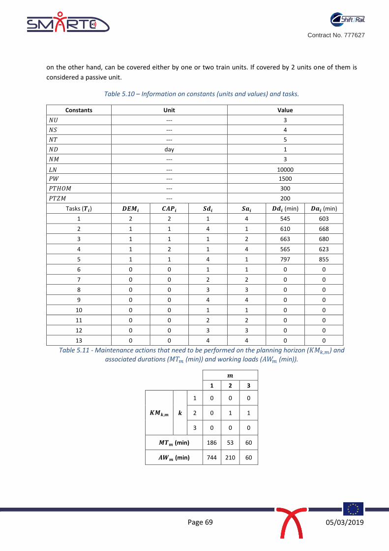
Page 69 05/03/2019
Contract No. 777627
on the other hand, can be covered either by one or two train units. If covered by 2 units one of them is
considered a passive unit.
Table 5.10 – Information on constants (units and values) and tasks.
Constants Unit Value
𝑁𝑈 --- 3
𝑁𝑆 --- 4
𝑁𝑇 --- 5
𝑁𝐷 day 1
𝑁𝑀 --- 3
𝐿𝑁 --- 10000
𝑃𝑊 --- 1500
𝑃𝑇𝐻𝑂𝑀 --- 300
𝑃𝑇𝑍𝑀 --- 200
Tasks (𝑻𝒊) 𝑫𝑬𝑴𝒊 𝑪𝑨𝑷𝒊 𝑺𝒅𝒊 𝑺𝒂𝒊 𝑫𝒅𝒊 (min) 𝑫𝒂𝒊 (min)
1 2 2 1 4 545 603
2 1 1 4 1 610 668
3 1 1 1 2 663 680
4 1 2 1 4 565 623
5 1 1 4 1 797 855
6 0 0 1 1 0 0
7 0 0 2 2 0 0
8 0 0 3 3 0 0
9 0 0 4 4 0 0
10 0 0 1 1 0 0
11 0 0 2 2 0 0
12 0 0 3 3 0 0
13 0 0 4 4 0 0
Table 5.11 - Maintenance actions that need to be performed on the planning horizon (𝐾𝑀𝑘,𝑚) and associated durations (𝑀𝑇𝑚 (min)) and working loads (𝐴𝑊𝑚 (min)).
𝒎
1 2 3
𝑲𝑴𝒌,𝒎 𝒌
1 0 0 0
2 0 1 1
3 0 0 0
𝑴𝑻𝒎 (min) 186 53 60
𝑨𝑾𝒎 (min) 744 210 60

Page 70 05/03/2019
Contract No. 777627
In Table 5.11, 𝑘 and 𝑚 are respectively the train units and maintenance actions. The parameter 𝐾𝑀𝑘,𝑚
equals to one when a maintenance action must be performed on a specific unit. Specifically, unit 2 must
perform two kinds of maintenance actions: 2 and 3. The other units have no planned maintenance actions
for the given time-period. Therefore, unit 2 must go to the depot at least once to satisfy the maintenance
requirements. This information is provided by a long-term maintenance plan regarding preventive
maintenance (i.e. it is considered an input). Table 5.11 also provides information on the different types of
maintenance actions, namely the duration of each maintenance action (𝑀𝑇𝑚 in min) and the working load
or amount of work (𝐴𝑊𝑚 in min).
The model is solved and it creates a data file with the information concerning the pairs of tasks that were
covered by each unit, the dead-headings that were performed and finally, the maintenance actions that
were executed and the days each unit spent in the depot for those maintenance actions. The displayed
information enables the rolling-stock planning for the given time period. The obtained rolling-stock
planning is outlined in Figure 5.8.
Several facts should be highlighted from the analysis of Figure 5.8. First, we can notice that every task and
maintenance action was successfully covered, with the need to make use of dead-headings. Train unit 1
(𝑈1) performs two tasks: 𝑇1 and 𝑇2. The pairs of tasks (6, 1) and (2, 10) are beginning and ending virtual
tasks, respectively and indicate that the row assigned to unit 𝑈1 starts and finishes at station 1 (Roma-
Areeiro). The link between 𝑇1 and 𝑇2 respects the minimal turning time of station 4 (𝑇𝑀4 = 1 𝑚𝑖𝑛), as
there is a 7-minute gap between the arrival time of task 1 (𝐷𝑎1 = 603 𝑚𝑖𝑛) and the departure time of task
2 (𝐷𝑑2 = 610 𝑚𝑖𝑛). As task 𝑇1 must be covered by two train units, train unit 3 also covers 𝑇1. Furthermore,
train unit 𝑈3 also covers 𝑇3. The pairs of tasks (6, 1) and (3, 11) are the beginning and ending virtual tasks,
Figure 5.8 – A 3-row-roster to cover timetable demand and maintenance requirements, including: virtual tasks (yellow dashed rectangle), real tasks (black rectangle), dead-headings (green dashed rectangle) and maintenance actions (red rectangle).
Page 71 05/03/2019
Contract No. 777627
respectively. In this case, row 3 (𝑅3) also starts at station 1 but ends at station 2 (Pragal). To link tasks 𝑇1 to
𝑇3, a dead-heading must be introduced, as the arrival station of 𝑇1 is Setúbal (𝑆𝑎1 = 4) and the departure
station of 𝑇3 is Roma-Areeiro (𝑆𝑑3 = 1). This dead-headind has a duration of 45 minutes, so it fits between
𝑇1 and 𝑇3, as 𝐷𝑑3 − 𝐷𝑎1 ≥ DW4,1, i.e. 663 − 603 = 60 ≥ 45 𝑚𝑖𝑛. Train unit 𝑈2 performs tasks 𝑇4 and
𝑇5. Again, the pair of tasks (6,4) and (5,10) are virtual tasks, indicating the stations where 𝑅2 begins and
ends. Two maintenance slots were added between the two tasks: 𝐾𝑀2,2 and 𝐾𝑀2,3. Both are performed
on the only day available (𝑑 = 1). Maintenance 𝑚 = 2 has a duration of 53 minutes (𝑀𝑇2 = 53 𝑚𝑖𝑛) and
maintenance 𝑚 = 3 has a duration of 60 minutes (𝑀𝑇3 = 60 𝑚𝑖𝑛). Since they are performed on the same
day, they must respect a 5-minute minimal interval between each other. It means that the two maintenance
actions take 118 minutes (53 + 5 + 60) to be performed in the depot. Furthermore, the train unit must
perform an empty run from the arrival station of 𝑇4 to the depot (W4,3) and another empty run from the
depot to the departure station of 𝑇5 (W3,4). Both empty runs have a duration of 21 minutes, so 42 minutes
are necessary to move train unit 2 for maintenance purposes. Therefore, a total of 160 minutes (42 +
118) are necessary to perform the maintenance actions, and it fits between tasks 𝑇4 and 𝑇5 , as
𝐷𝑑5 − 𝐷𝑎4 = 797 − 623 = 174 ≥ 160 𝑚𝑖𝑛. Finally, the working loads of the maintenance actions are:
𝐴𝑊2 = 210 𝑚𝑖𝑛 and 𝐴𝑊3 = 60 𝑚𝑖𝑛, which summed up are equal to 270 minutes of work needed.

Page 72 05/03/2019
Contract No. 777627
6. DISCUSSION AND CONCLUSIONS
Maintenance is a combination of actions carried out to retain an item in, or restore it to, an acceptable
condition in a cost effective manner (Williams et al. 1994). There are two main maintenance
strategies: corrective and preventive maintenance. Corrective maintenance is a maintenance strategy by
which maintenance actions are carried out after failure detection and is aimed at restoring an asset to a
condition in which it can perform its intended function. In contrast, preventive maintenance is a strategy
by which maintenance, including tests, measurements, adjustments, and care/servicing, are performed
specifically to prevent faults from occurring or developing to a major defect.
A preventive maintenance strategy can be either consist of periodical maintenance, which allows periodical
scheduling of convenient maintenance to prevent unexpected equipment failures or condition based
(on-condition) maintenance, by which maintenance actions are undertaken only when the component or
system reaches a particular state or condition. Figure 6.1 illustrates the different types of maintenance
strategies.
Figure 6.1: Different maintenance strategies
Condition-based Maintenance (CBM) allows the replacement of rolling stock components at the right point
to maximise the life of the component or where continued use would result in an increased operating cost
and potential in-service failures. In this case CBM would result in the lowest life cycle cost among the
different strategies. The life cycle cost (LCC) of a rolling stock is the sum of initial cost, operating cost,
inspection cost and maintenance cost, divided by life of the component. This can be calculated as follows.
𝐿𝐶𝐶 = 𝐶𝑖𝑛𝑖𝑡 + 𝐶𝑜𝑝 + 𝐶𝑖𝑛𝑠𝑝 + 𝐶𝑚𝑎𝑖𝑛 + 𝐶𝑓𝑎𝑖𝑙
𝑇𝑙𝑖𝑓𝑒𝑠𝑝𝑎𝑛
where LCC is the life cycle cost for a component; 𝐶𝑖𝑛𝑖𝑡 is the cost used to purchase and install the
component when it was new; 𝐶𝑜𝑝 is the additional operating cost due to the component; 𝐶𝑖𝑛𝑠𝑝 is the cost
associated with inspection and detection for the maintenance policy; 𝐶𝑚𝑎𝑖𝑛 is the cost associated with the
repair/replacement of the component; and 𝐶𝑓𝑎𝑖𝑙 is the cost caused by the failure of the component.

Page 73 05/03/2019
Contract No. 777627
Commercial aviation industry was the first industry to systematically confront the challenges faced in
operation and maintenance. A comprehensive maintenance decision-making process, known within
aviation industry as MSG-3 and outside as Reliability-Centred Maintenance (RCM), was developed. In
Section 2 of this report, the techniques used within the MSG-3 methodology to determine the appropriate
maintenance actions was demonstrated through application to a HPV system. This has illustrated how the
process could be applied for the future maintenance planning of rolling stock components/systems and
support the implementation of ‘Smart Rolling Stock Maintenance’. The use of the MSG-3 decision logic was
shown to help to identify whether a time- or condition-based maintenance approach is appropriate for each
maintenance significant item. These techniques will be considered when applying CBM to selected rolling
stock components/systems during Task 2.4 of WP2 of the SMaRTE project.
The acquisition, storage, transmission and processing of data is a key element of the CBM system. The issues
relating to the interoperability of data within a CBM system have been discussed in Section 3 of this report,
along with the characteristics of typical condition data. A data model for the CBM system is proposed using
an ontology approach which ensures that the data within the system is interoperable.
In the CBM system; condition data is potentially acquired from multiple sources and is used in prognosis
algorithms to predict future failures of a system. These data processing algorithms are the foundations of
the CBM system and three critical challenges have been identified:
the determination of system health indicator
the accuracy and interval of condition monitoring
the determination of condition limits
A key requirement to overcoming these challenges is to obtain the right information in the right time. In
the SMaRTE project various data processing and feature extraction techniques have been explored from a
data engineering perspective and these will be applied to a range of case studies during Task 2.4 and
reported in Deliverable 2.3.
A CBM system for rolling stock does not just consist of techniques for the post-processing of condition data
but also techniques to support maintenance decision making, with the overall goal of reducing the LCC of
the system. The maintenance decision support system can be a computerised information system which
contains specific knowledge of rolling stock maintenance and analytical decision models to assist the
decision maker by presenting information and the interpretation of various alternatives. There is a very
large literature on maintenance methods, philosophies and strategies. The maintenance management
systems for rolling stock proposed in this report must take into account technical and operational
constraints in order to plan and schedule maintenance actions in a given time window. In addition,
maintenance of different fleets operated in a company requires more careful planning and efficient
management of resources. In Tasks 2.2 and 2.3, Integer Linear Programming (ILP) models were used to
develop tactical planning and operational maintenance scheduling models. These models will be applied to
a detailed case study in Task 2.4 and the results reported in Deliverable 2.3.

Page 74 05/03/2019
Contract No. 777627
7. REFERENCES
Afwan, M., Memon, M., Pawar, Y., and Kainge, S.B. (2017) A Study on Landing Gear Arrangement of n
Aircraft. International Journal of Innovative Research in Science, Engineering and Technology, 6 (8): pp
15730- 15737.
Ahmadi, A., & Kumar, U. (2011). Cost based risk analysis to identify inspection and restoration intervals of
hidden failures subject to aging. IEEE Transactions on Reliability, 60(1): pp197-209.
Ahmadi, A., Soderholm, P. and Kumar, U. (2010), On aircraft scheduled maintenance program
development, Journal of Quality in Maintenance Engineering, 16 (3): pp. 229-255.
ATA MSG-3, (2007), Operator/Manufacturer Scheduled Maintenance Development, Air Transport
Association of America, Washington, DC.
Aviation safety bureau-Chapter 12. Hydraulic and Pneumatic Power Systems: www.aviation-safety-
bureau.com
MIL-STD-2173, (1986), Reliability Centered Maintenance. Washington D.C.: Department of Defense.
Moubray, J., (1997), Reliability Centered Maintenance. Oxford: Butterworth-Heinemann.
Nowlan, F.S. and Heap, H.F., (1978), Reliability Centered Maintenance, Springfield: National Technical
Information Service (NTIS), USA.
SAE JA1012, (2002), A Guide to the Reliability-Centered Maintenance (RCM) Standard, the Engineering
Society for Advancing Mobility Land Sea Air and Space, USA.
Tsang, A., (1995), Condition Based Maintenance tools and decision-making. Journal of Quality in
Maintenance Engineering 1(3): pp3-17.
Wang, S., Tomovic, M., & Liu, H. (2015). Commercial Aircraft Hydraulic Systems: Shanghai Jiao Tong
University Press Aerospace Series. Academic Press.
www.flight-mechanic.com, hydraulic-power-systems-valves-part-two. Aircraft Landing Gear Systems
IEC (2004), IEC 60300-3-14:2004 Standard | Dependability management – Part 3-14: Application Guide –
Maintenance and maintenance support.
IEEE (1990), IEEE Standard Computer Dictionary: A compilation of IEEE standard computer glossaries, New
York, NY, 1990
Nash, A., Huerlimann, D., Schuette, J., and Krauss, V. (2004) “RailML-a standard data interface for railroad
applications.” WIT press.
UIC (2013), “RailTopoModel – Railway Network Description”, <https://www.railtopomodel.org/en/>
InteGRail (2011), “InteGRail – Intelligent Integration of Railway Systems”, <http://www.integrail.info>
Jardine, A.K., Lin, D., and Banjevic, D., (2006). A review on machinery diagnostics and prognostics
implementation condition-based maintenance. Mechanical Systems and Signal Processing, vol 20, no 7,
pp 1483-1510, 2006.
Si, X. -S., Wang, W., Hu, C. -H., and Zhou, D. -H, Remaining useful life estimation – a review on the
statistical data driven approaches. European Journal of Operational Research, vol 213, no. 1, pp. 1-14,
2011
Sikorska J.Z., Hodkiewicz, M., and Ma, L., Prognostic modelling options for remaining useful life estimation
by industry, Mechanical Systems and Signal Processing, vol 25, no 5, pp 1803-1836, 2011.

Page 75 05/03/2019
Contract No. 777627
Gaber M.M., Zaslavshy, A., and Krishnaswamy, S., Mining data streams: a review. SIGMOD Record, vol 34,
no 2, pp 18-26, 2005.
Famili, A., Shen, W.-M., Weber, R., and Simoudis, E., Data processing and intelligent data analysis,
Intelligent Data Analysis, vol 1, no 1, pp 3-23, 1997.
Trier, Ø. D., Jain, A. K., and Taxt, T, Feature extraction methods for character recognition-A survey, Pattern
Recognition, vol 29, no 4, pp 641-662, 1996.
Ghasemi, A., Yacout, S., and Ouali, M.-S., Parameter estimation methods for condition-based
maintenance with indirect observations, IEEE Transaction on Reliability, vol 59, no 2, pp 426-439, 2010.
Waibel, A., Hanazawa, T., Hinton, G., Shikano, K., and Lang, K., Phoneme recorgnition using time-delay
neural networks, IEEE transactions on acoustics, speech, and signal processing, vol 37, no 3, pp 328-339,
1989.
Narendra K.S., Parthasarathy, K., Identification and control of dynamical systems using neural networks.
IEEE transaction on neural network, vol 1, no 1, pp 4-27, 1990.
Bazargan, M. (2015). An optimization approach to aircraft dispatching strategy with maintenance cost–A
case study. Journal of Air Transport Management, 42, 10-14.
Binder, S., Maknoon, Y., & Bierlaire, M. (2017). The multi-objective railway timetable rescheduling
problem. Transportation Research Part C: Emerging Technologies, 78, 78-94.
Bohlin, M., & Wärja, M. (2015). Maintenance optimization with duration-dependent costs. Annals of
Operations Research, 224(1), 1-23.
Cacchiani, V., Huisman, D., Kidd, M., Kroon, L., Toth, P., Veelenturf, L., & Wagenaar, J. (2014). An overview
of recovery models and algorithms for real-time railway rescheduling. Transportation Research Part B:
Methodological, 63, 15-37.
Caprara, A., Monaci, M., Toth, P., & Guida, P. L. (2006). A Lagrangian heuristic algorithm for a real-world
train timetabling problem. Discrete applied mathematics, 154(5), 738-753.
Cordeau, J. F., Desaulniers, G., Lingaya, N., Soumis, F., & Desrosiers, J. (2001). Simultaneous locomotive
and car assignment at VIA Rail Canada. Transportation Research Part B: Methodological, 35(8), 767-787.
Doganay, K., & Bohlin, M. (2010). Maintenance plan optimization for a train fleet. WIT Transactions on
The Built Environment, 114(12), 349-358.
Forsgren, M., Aronsson, M., & Gestrelius, S. (2013). Maintaining tracks and traffic flow at the same time.
Journal of Rail Transport Planning & Management, 3(3), 111-123.
Gabrel, V., Murat, C., & Thiele, A. (2014). Recent advances in robust optimization: An overview. European
journal of operational research, 235(3), 471-483.
Giacco, G. L., D’Ariano, A., & Pacciarelli, D. (2014). Rolling stock rostering optimization under maintenance
constraints. Journal of Intelligent Transportation Systems, 18(1), 95-105.
Haghani, A., & Shafahi, Y. (2002). Bus maintenance systems and maintenance scheduling: model
formulations and solutions. Transportation research part A: Policy and Practice, 36(5), 453-482.
Huisman, D., Kroon, L. G., Lentink, R. M., & Vromans, M. J. (2005). Operations research in passenger
railway transportation. Statistica Neerlandica, 59(4), 467-497.
Lai, Y. C. R., Wang, S. W., & Huang, K. L. (2017). Optimized Train-Set Rostering Plan for Taiwan High-Speed
Rail. IEEE Transactions on Automation Science and Engineering, 14(1), 286-298.

Page 76 05/03/2019
Contract No. 777627
Lidén, T., & Joborn, M. (2016). Dimensioning windows for railway infrastructure maintenance: Cost
efficiency versus traffic impact. Journal of Rail Transport Planning & Management, 6(1), 32-47.
Luan, X., Miao, J., Meng, L., Corman, F., & Lodewijks, G. (2017). Integrated optimization on train
scheduling and preventive maintenance time slots planning. Transportation Research Part C: Emerging
Technologies, 80, 329-359.
Maróti, G., & Kroon, L. (2005). Maintenance routing for train units: the transition model. Transportation
Science, 39(4), 518-525.
Maróti, G., & Kroon, L. (2007). Maintenance routing for train units: The interchange model. Computers &
Operations Research, 34(4), 1121-1140.
Maróti, G., & Kroon, L. G. (2004). Maintenance routing for train units: the scenario model. CWI.
Probability, Networks and Algorithms [PNA], (E 0414).
Papakonstantinou, K. G., & Shinozuka, M. (2014). Planning structural inspection and maintenance policies
via dynamic programming and Markov processes. Part I: Theory. Reliability Engineering & System Safety,
130, 202-213.
Pathak, S., Ábrahám, E., Jansen, N., Tacchella, A., & Katoen, J. P. (2015, April). A greedy approach for the
efficient repair of stochastic models. In NASA Formal Methods Symposium (pp. 295-309). Springer, Cham.
Peng, F., Ouyang, Y., & Somani, K. (2013). Optimal routing and scheduling of periodic inspections in large-
scale railroad networks. Journal of Rail Transport Planning & Management, 3(4), 163-171.
Puterman, M. L. (2014). Markov decision processes: discrete stochastic dynamic programming. John Wiley
& Sons.
Santos, R., Teixeira, P. F., & Antunes, A. P. (2015). Planning and scheduling efficient heavy rail track
maintenance through a Decision Rules Model. Research in Transportation Economics, 54, 20-32.
Sheskin, T. J. (2016). Markov chains and decision processes for engineers and managers. CRC Press.
Tréfond, S., Billionnet, A., Elloumi, S., Djellab, H., & Guyon, O. (2017). Optimization and simulation for
robust railway rolling-stock planning. Journal of Rail Transport Planning & Management, 7(1-2), 33-49.
Veelenturf, L. P., Kidd, M. P., Cacchiani, V., Kroon, L. G., & Toth, P. (2015). A railway timetable rescheduling approach for handling large-scale disruptions. Transportation Science, 50(3), 841-862.

Page 77 05/03/2019
Contract No. 777627
APPENDIX A: FAILURE EFFECT CATEGORY

Page 78 05/03/2019
Contract No. 777627
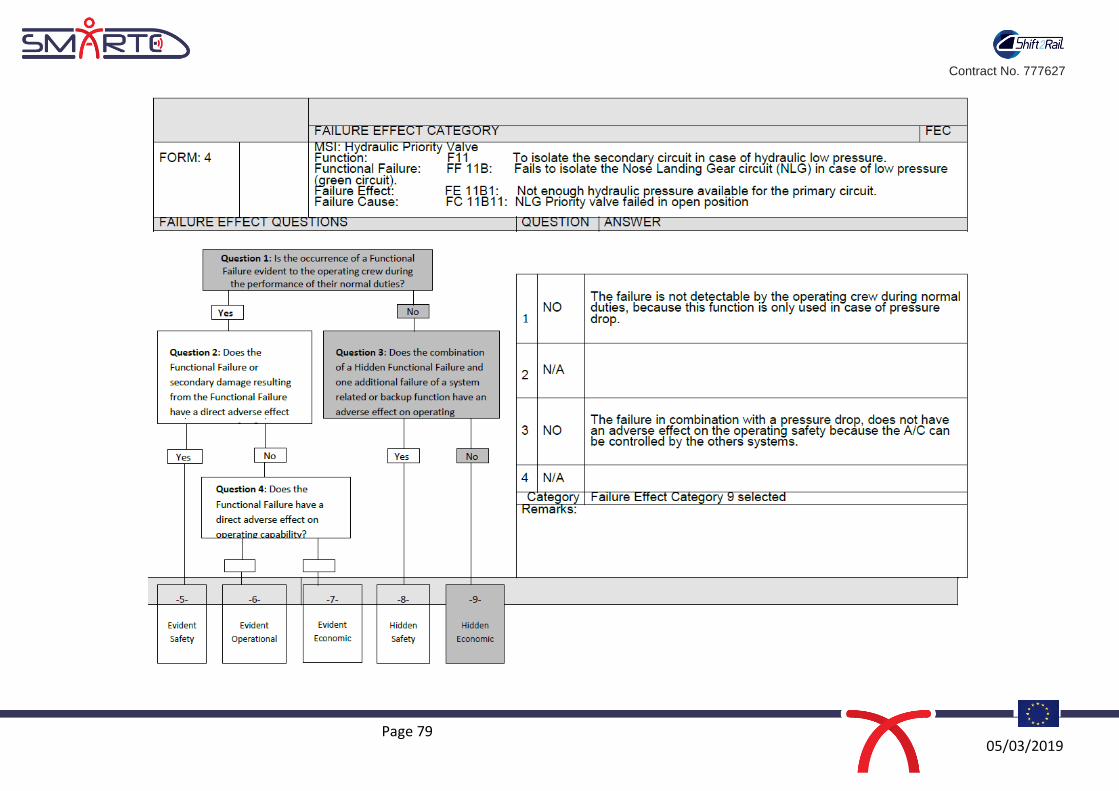
Page 79 05/03/2019
Contract No. 777627

Page 80 05/03/2019
Contract No. 777627

Page 81 05/03/2019
Contract No. 777627
Figure 3: MSG-3 Logic Diagram for Systems and Power plant (ATA MSG-3, 2007)

Page 82 DD/MM/YYYY
Contract No. 777627
Figure 4: MSG-3 Applicability and Effectiveness criteria for task selection (ATA MSG-3, 2007)


![EXPO RAIL OPERATIONS AND MAINTENANCE · PDF file01 78 43 SPARE PARTS AND REPLACEMENT MATERIALS [EXPO] ... Expo Rail Operations and Maintenance Facility TABLE OF](https://img.dokumen.tips/doc/110x75/5a8091c47f8b9a0c748c7b20/expo-rail-operations-and-maintenance-78-43-spare-parts-and-replacement-materials.jpg)