Embed Size (px)
Citation preview

2004-39Final Report
SMALL STRAIN AND RESILIENT MODULUS TESTING OF GRANULAR
SOILS
Technical Report Documentation Page 1. Report No. 2. 3. Recipients Accession No. 2004-39 4. Title and Subtitle 5. Report Date
August 2004 6.
SMALL STRAIN AND RESILIENT MODULUS TESTING OF GRANULAR SOILS
7. Author(s) 8. Performing Organization Report No. Peter Davich, Joseph Labuz, Bojan Guzina & Andrew Drescher 9. Performing Organization Name and Address 10. Project/Task/Work Unit No.
11. Contract (C) or Grant (G) No.
Department of Civil Engineering University of Minnesota 500 Pillsbury Drive S.E. Minneapolis, Minnesota 55455-0220
(c) 81655 (w) 32
12. Sponsoring Organization Name and Address 13. Type of Report and Period Covered Final Report 14. Sponsoring Agency Code
Minnesota Department of Transportation Research Services Section 395 John Ireland Boulevard Mail Stop 330 St. Paul, Minnesota 55155
15. Supplementary Notes www.lrrb.org/PDF/200439.pdf 16. Abstract (Limit: 200 words) Resilient modulus, shear strength, dielectric permittivity, and shear and compressional wave speed values were determined for 36 soil specimens created from the six soil samples. These values show that the soils had larger stiffnesses at low moisture contents. It was also noted during testing that some non-uniformity was present within the axial displacement measurements; larger levels of non-uniformity were associated with low moisture contents, possibly due to more heterogeneous moisture distributions within these specimens. Lastly, the data collected during this study was used to recommend a relationship between granular materials’ small strain modulus and their resilient modulus. This relationship was given in the form of a hyperbolic model that accurately represents the strain-dependent modulus reduction of the base and subgrade materials. This model will enable field instruments that test at small strains to estimate the resilient modulus of soil layers placed during construction.
17. Document Analysis/Descriptors 18. Availability Statement Bender element testing Resilient modulus testing
Select granular soil No restrictions. Document available from: National Technical Information Services, Springfield, Virginia 22161
19. Security Class (this report) 20. Security Class (this page) 21. No. of Pages 22. Price Unclassified Unclassified 117
Small Strain and Resilient Modulus Testing of Granular Soils
Final Report
Prepared by:
Peter Davich Joseph F. Labuz Bojan Guzina
Andrew Drescher
Department of Civil Engineering University of Minnesota
August 2004
Published by:
Minnesota Department of Transportation Research Services Section
395 John Ireland Boulevard, Mail Stop 330 St. Paul, Minnesota 55155
This report represents the results of research conducted by the authors and does not necessarily represent the views or policies of the Minnesota Department of Transportation and/or the Center for Transportation Studies. This report does not contain a standard or specified technique. The authors and the Minnesota Department of Transportation and/or Center for Transportation Studies do not endorse products or manufacturers. Trade or manufacturers’ names appear herein solely because they are considered essential to this report.
Table of Contents
Chapter 1 – Introduction............................................................................................................... 1
1.1 Resilient Modulus....................................................................................................... 2
1.2 Small Strain Testing.................................................................................................... 3
1.3 Organization................................................................................................................ 4
Chapter 2 – Literature Review...................................................................................................... 5
2.1 Resilient Modulus Testing.......................................................................................... 5
2.1.1 Long Term Pavement Performance Protocol P46....................................... 6
2.1.2 Equipment Modifications............................................................................. 8
2.2 Bender Element Testing.............................................................................................. 9
2.2.1 Density Effects........................................................................................... 10
2.2.2 Wave Speed Effects................................................................................... 11
2.2.3 Research Recommendations...................................................................... 12
Chapter 3 – Test Procedure......................................................................................................... 13
3.1 Test Equipment......................................................................................................... 13
3.1.1 Triaxial Cell............................................................................................... 13
3.1.2 Load Cell and LVDTs................................................................................ 16
3.1.3 Bender Element System.............................................................................1 7
3.1.4 Load Frame................................................................................................ 19
3.2 Soil Samples..............................................................................................................19
3.3 Specimen Preparation............................................................................................... 21
3.3.1 Compaction................................................................................................ 23
3.3.2 Percometer Measurements......................................................................... 25
3.3.3 Bender Element Protection........................................................................ 26
3.4 Specimen Testing...................................................................................................... 27
3.4.1 Resilient Modulus Test.............................................................................. 28
3.4.2 Shear Strength Test.................................................................................... 31

Chapter 4 – Discussion of Results.............................................................................................. 33
4.1 Testing Schedule....................................................................................................... 33
4.2 Resilient Modulus Data Interpretation...................................................................... 34
4.2.1 Sample Calculation.................................................................................... 36
4.2.2 Deformation Homogeneity........................................................................ 36
4.3 Bender Element Data Interpretation......................................................................... 41
4.3.1 Cross Correlation....................................................................................... 44
4.3.2 Sample Calculation.................................................................................... 47
4.4 Test Data................................................................................................................... 48
4.4.1 Resilient Modulus Data..............................................................................48
4.4.2 Bender Element Data................................................................................. 53
4.4.3 Percometer Data......................................................................................... 59
4.4.4 Shear Strength Data................................................................................... 63
4.5 Degradation Curves.................................................................................................. 66
Chapter 5 – Summary and Conclusions...................................................................................... 70
References................................................................................................................................... 72
Appendix A................................................................................................................................. A-1
Appendix B................................................................................................................................. B-1
Appendix C................................................................................................................................. C-1
Appendix D................................................................................................................................. D-1
Appendix E.................................................................................................................................. E-1

List of Figures
1.1. Modulus Variation With Strain Level................................................................................... 3
2.1. LTPP P46 Load History........................................................................................................ 6
2.2. Bender Element Wave Generation........................................................................................ 9
3.1. Triaxial Cell Diagram......................................................................................................... 14
3.2. Triaxial Cell Containing Specimen..................................................................................... 15
3.3. Bender Element Incorporation Within Platen..................................................................... 16
3.4. Load Cell............................................................................................................................. 16
3.5. LVDT Collars with Spacers................................................................................................ 17
3.6. Bender Element Cantilever Strip........................................................................................ 18
3.7. Load Frame......................................................................................................................... 19
3.8. Labeled Soil Samples.......................................................................................................... 20
3.9. Oversized Aggregate........................................................................................................... 21
3.10. Tempering Container........................................................................................................ 22
3.11. Compaction Data for Sample A........................................................................................ 23
3.12. Stages of Specimen Preparation........................................................................................ 24
3.13. Percometer Measurement.................................................................................................. 25
3.14. Bender Element Protection System.................................................................................. 26
3.15. Stages of Element Protection............................................................................................ 27
3.16. Specimen Loaded within Triaxial Cell............................................................................. 28
3.17. Fluid Pressure Transducer................................................................................................. 29
3.18. MR Test Displacement History......................................................................................... 30
3.19. P-Wave Source and Receiver Time Histories................................................................... 31
3.20. Specimen Failure.............................................................................................................. 32
4.1. Displacement Histories....................................................................................................... 38
4.2. α-Value Variation............................................................................................................... 40
4.3. Deviator Stress and Deformation Homogeneity................................................................. 41
4.4. Identification of Wave Arrivals.......................................................................................... 42
4.5. P-Wave Cross Correlation Results...................................................................................... 45
4.6. S-Wave Cross Correlation Results...................................................................................... 46
4.7. Resilient Modulus Data.......................................................................................................51
4.8. MR Versus Mean Stress for Sample A................................................................................ 53
4.9. MR and EMAX Curves.......................................................................................................... 54
4.10. Bender Element Data......................................................................................................... 55
4.11. Data used in Dielectric-Moisture Relationship................................................................. 61
4.12. Ultimate Shear Strength.................................................................................................... 66
4.13. Hyperbolic Predictions of Cyclic Triaxial Results........................................................... 68
A.1. Gradations for Samples.................................................................................................... A-2
A.2. Soil-Water Characteristic Curve for Sample A.............................................................. A-3
A.3. Soil-Water Characteristic Curve for Sample D............................................................... A-3
A.4. Soil-Water Characteristic Curve for Sample F............................................................... A-4
A.5. Soil-Water Characteristic Curve for Sample H............................................................... A-4
A.6. Soil-Water Characteristic Curve for Sample J................................................................ A-5
A.7. Soil-Water Characteristic Curve for Sample N............................................................... A-5
D.1. Young’s Modulus Data from Sample A......................................................................... D-2
D.2. Young’s Modulus Data from Sample D......................................................................... D-3
D.3. Young’s Modulus Data from Sample F........................................................................... D-4
D.4. Young’s Modulus Data from Sample H.......................................................................... D-5
D.5. Young’s Modulus Data from Sample J............................................................................D-6
D.6. Young’s Modulus Data from Sample N.......................................................................... D-7
D.7. Resilient Modulus Versus Confining Pressure Data........................................................ D-8
D.8. Resilient Modulus and Mean Stress Data from Sample A............................................ D-11
D.9. Resilient Modulus and Mean Stress Data from Sample D............................................ D-12
D.10. Resilient Modulus and Mean Stress Data from Sample F........................................... D-13
D.11. Resilient Modulus and Mean Stress Data from Sample H.......................................... D-14
D.12. Resilient Modulus and Mean Stress Data from Sample J............................................ D-15
D.13. Resilient Modulus and Mean Stress Data from Sample N.......................................... D-16
E.1. Resilient Modulus Values from both Protocols................................................................ E-5
E.2. NCHRP 1-28A and Bender Element Moduli................................................................... E-6
List of Tables
2.1. LTPP P46 Loading Sequences.............................................................................................. 7
3.1. Soil Sample Data................................................................................................................. 20
4.1. Test Matrix.......................................................................................................................... 34
4.2. MR Test α Values................................................................................................................ 39
4.3. Wave Speeds at Variable Pulse Frequencies...................................................................... 43
4.4. Target and Measured Specimen Preparation Parameters.................................................... 48
4.5. Resilient Modulus and EMAX................................................................................................ 57
4.6. Elastic Parameters Estimated from Bender Element Testing.............................................. 58
4.7. Dielectric Permittivity and Conductivity............................................................................ 60
4.8. Dielectric Moisture Content Estimates............................................................................... 62
4.9. Deviator Stress Values at Shear Failure.............................................................................. 63
4.10. Cohesion and Friction Angle of Samples......................................................................... 65
A.1. Soil Gradation Data......................................................................................................... A-1
B.1. Phase Angles for Test System.......................................................................................... B-1
B.2. Load and Displacement Measurements for University’s Load Frame............................. B-3
B.3. Load Measurements for Mn/DOT’s Load Frame............................................................ B-4
Executive Summary
Resilient modulus testing measures the mechanical response of a pavement base or subgrade soil
to a cyclic load simulating traffic. The resilient modulus values measured during the test are
commonly used as design parameters for pavement structures. In addition, a new generation of
small-strain tests have recently been developed to aid the quality assurance during pavement
construction. The purpose of this study is to compare the small strain modulus and resilient
modulus of pavement foundation materials in the context of resilient modulus testing.
Thirty-six resilient modulus tests were performed on samples of six soils that are
commonly used within pavement structures in Minnesota. These tests were performed at three
different values of moisture content for each soil; one repetition of each test was carried out to
investigate the repeatability of the data. To provide the data necessary to link the small-strain
modulus to the resilient modulus, a sequence of bender element tests was performed on the soil
specimens during each resilient modulus test.
Resilient modulus, ultimate shear strength, dielectric permittivity, and shear and
compressional wave speed values were determined for 36 soil specimens created from the six
soil samples. These values show that the soils had larger stiffnesses at low moisture contents. It
was also noted during testing that some non-uniformity was present within the axial
displacement measurements during testing; larger levels of non-uniformity were associated with
low moisture contents, possibly due to more heterogeneous moisture distributions within these
specimens. Lastly, the data collected during this study was used to recommend a relationship
between granular materials’ small strain modulus and their resilient modulus. This relationship
was given in the form of a hyperbolic model that accurately represents the strain-dependent
modulus reduction of the base and subgrade materials. This model will enable field instruments
that test at small strains to estimate the resilient modulus of soil layers placed during
construction.

1
Chapter 1 Introduction
Asphalt and concrete pavements rest on one or more layers of engineered soil. The overall
stiffness of the pavement structure is greatly affected by the composition of these foundation
layers, which are most often composed of soils containing primarily gravel and sand. Owing to
the critical effect that the foundation layers have on the overall stiffness of the pavement
structure, it is important to understand how these soils behave under traffic loading.
One of the most commonly used parameters that describe the foundation soil stiffness is
the resilient modulus (MR), which is a measure of the degree to which a soil can recover from
stress levels commonly placed upon roadbed soils by traffic. Many pavement engineering firms
and agencies, including the Minnesota Department of Transportation (Mn/DOT), currently use
MR values as a measure of the base and subgrade stiffnesses in their pavement design
procedures.
Unfortunately, many pavements fail before the end of their predicted design life. There
are a variety of causes for this, but one of the most common is poor construction. As a result, the
importance of quality control procedures is being emphasized more than ever. One of the
difficulties in determining the quality of base layer compaction is that it is impossible to directly
measure a soil’s MR at a construction site. The resilient modulus test can only be performed in a
laboratory, and taking core samples from the compacted soil is both time-consuming and harmful
to the pavement under construction. As a result, it is difficult to determine if the base layers at a
construction site have the MR values that are required by the pavement design. Therefore, a
fundamental relationship between the resilient modulus values and quantities that can be
measured in the field (e.g. small-strain modulus) would be an indispensible tool to elevate the
quality of pavements.
Partially in response to this need, Mn/DOT recently initiated a series of studies designed
to test the stiffness properties of base layers in the field. Several of these projects, such as the
portable deflectometer study carried out by Hoffmann et al.[1], deal with instruments designed to
measure the small strain modulus of in-situ soils undergoing small mechanical vibration. Many
of these projects were successful in developing or creating test protocols for instrumentation that

2
can measure small strain modulus values using non-destructive wave sources. The objective of
this study is to link the small strain modulus values of pavement foundation layers obtained from
small strain testing to their MR counterparts obtained in the laboratory. An accurate correlation
between these parameters would enable better monitoring of base properties during construction
and, ultimately, reduce the number of premature pavement failures.
1.1 Resilient Modulus
Many highway departments use the resilient modulus as one of the primary parameters in their
pavement design procedures. One test protocol for measuring MR is Long Term Pavement
Protocol (LTPP) P46, which was developed by the Strategic Highway Research Program
(SHRP) [2]. A revised version of this protocol, the National Cooperative Highway Research
Program (NCHRP) 1-28 A, was released in 2002 [3]. It is different from LTPP P46 in many
ways; one of the most significant is that it involves larger stresses on specimens. These stresses
are large enough to cause the failure of some soils. In addition, NCHRP 1-28A has yet to be
widely implemented and the majority of existing MR data was generated using LTPP P46. For
these reasons, it was decided that LTPP P46 would be used for the purposes of this research. For
completeness, however, one MR test using the NCHRP 1-28A protocol was performed during the
course of this study to compare the moduli values resulting from the two testing procedures.
The LTPP P46 test protocol revolves around the cyclic triaxial testing of a soil specimen.
Each test cycle consists of a loading portion as well as time for material recovery. The load path
consists of an axial, haversine load pulse 0.1 s in duration. This is followed by 0.9 s of material
recovery for a total cycle time of 1 s. This cycle is intended to simulate the passing of one axle
over a pavement followed by a period of rest before the next axle. It is repeated 100 times while
the applied load and deformation of the specimen are measured. This loading sequence is
repeated 15 times at different values of confining pressure and deviator stress. The resilient
modulus values are calculated by dividing the cyclic axial stress by the recoverable axial strain.
The LTPP P46 protocol will be explained in further detail in section 2.1.1 of this report.
3
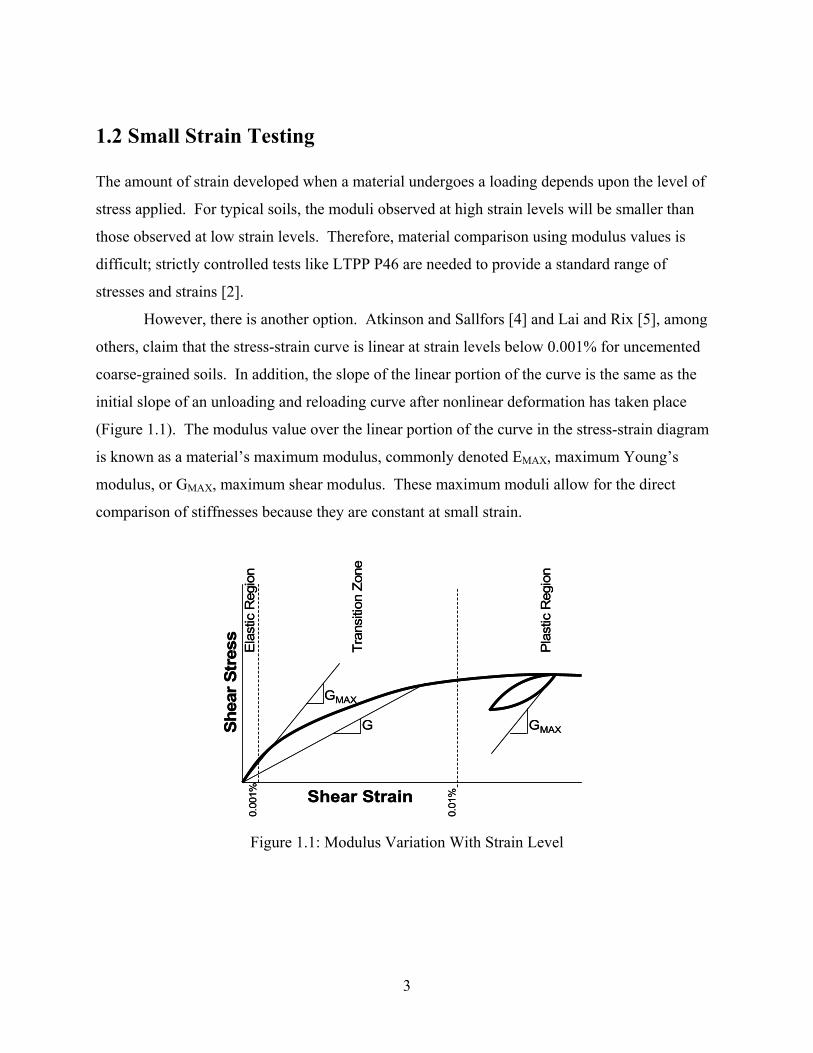
1.2 Small Strain Testing
The amount of strain developed when a material undergoes a loading depends upon the level of
stress applied. For typical soils, the moduli observed at high strain levels will be smaller than
those observed at low strain levels. Therefore, material comparison using modulus values is
difficult; strictly controlled tests like LTPP P46 are needed to provide a standard range of
stresses and strains [2].
However, there is another option. Atkinson and Sallfors [4] and Lai and Rix [5], among
others, claim that the stress-strain curve is linear at strain levels below 0.001% for uncemented
coarse-grained soils. In addition, the slope of the linear portion of the curve is the same as the
initial slope of an unloading and reloading curve after nonlinear deformation has taken place
(Figure 1.1). The modulus value over the linear portion of the curve in the stress-strain diagram
is known as a material’s maximum modulus, commonly denoted EMAX, maximum Young’s
modulus, or GMAX, maximum shear modulus. These maximum moduli allow for the direct
comparison of stiffnesses because they are constant at small strain.
Figure 1.1: Modulus Variation With Strain Level
Shear Strain
Shea
r Str
ess
GMAX
Ela
stic
Reg
ion
Tran
sitio
n Zo
ne
Pla
stic
Reg
ion
0.00
1%
0.01
%
GMAXG
Shear Strain
Shea
r Str
ess
GMAX
Ela
stic
Reg
ion
Tran
sitio
n Zo
ne
Pla
stic
Reg
ion
0.00
1%
0.01
%
GMAXG

4
A laboratory method for testing these small strain moduli is the bender element. There
are several different variations of bender elements currently being used, but the concept behind
each apparatus is the same. Two small elements are inserted into opposite faces of a soil
specimen. One of these elements is electrically excited and it produces small-strain shear and
compressional waves that travel through the specimen. The element on the opposite side of the
specimen receives the wave and the time history is recorded. After identifying the arrival times
of the shear and compressional waves, it is possible to calculate Poisson’s ratio and shear
modulus of the soil being tested. The bender element system used in this study will be further
detailed in section 3.1.2; the equations used in featured calculations are listed in section 4.3.
1.3 Organization
This report presents the results of the resilient modulus and small-strain bender element testing
of several soils. Chapter 2 reviews the literature pertaining to the design and usage of a triaxial
cell and bender element system. Chapter 3 contains a detailed description of the experimental
setup and a summary of test procedures. Chapter 4 focuses on the discussion of test results.
Chapter 5 summarizes and concludes the findings of this research.

5
Chapter 2 Literature Review
In recent years several protocols have been developed to measure the resilient modulus and small
strain modulus values of soils. These quantities have been used in conjunction with pavement
design and quality control processes. As a result, pavement engineering firms and agencies have
devoted many resources toward the investigation of these quantities. Many of these studies
recommend improvements to the testing apparatus and data interpretation algorithms. Their
findings will be discussed as they relate to this research.
2.1 Resilient Modulus Testing
The concept of the resilient modulus was developed by the Strategic Highway Research Program
in 1987. In subsequent years, several test protocols were suggested and discarded as
implementation problems arose. Then, in 1996, the Federal Highway Administration (FHWA)
set forth a standard protocol for MR testing known as Long Term Pavement Performance
Protocol P46 [2]. At this point, many pavement engineers were sufficiently convinced of the
usefulness of the MR parameter to acquire their own MR test systems. A large amount of MR
data was produced and used in the late 1990s as the parameter became more heavily involved in
pavement design processes.
In 2002 a new protocol, the National Cooperative Highway Research Program (NCHRP)
1-28A, was released to improve upon the old protocol [3]. There were several differences
between the procedures. For example, NCHRP 1-28A has a larger number of test sequence
variations for different soil classifications and the load pulse that simulates a traffic loading is
lengthened from 0.1 s to 0.2 s. However, the primary difference for granular soils (which will be
used in this study) is the number of loading sequences carried out; LTPP P46 requires cyclic
testing at 15 different combinations of confining pressure and deviator stress while NCHRP 1-
28A requires 30. In addition, NCHRP 1-28A requires deviator stress values much larger than
those used by LTPP P46.

6
The decision was made to use LTPP P46 for this study. However, one MR test was
performed using NCHRP 1-28A to compare the modulus values. The results of this test, as well
as itemized procedures from both protocols, are included in Appendix E.
2.1.1 Long Term Pavement Performance Protocol P46
LTPP P46 requires that the resilient modulus values of a soil specimen be determined by
performing dynamic triaxial testing on a cylindrical soil specimen [2]. A haversine load pulse
0.1 s in duration simulates the passing of an axle over a pavement. This load pulse is followed
by a 0.9 s period in which only a seating load equal to 10% of the peak stress is applied to the
specimen while the soil recovers from the loading. An example segment of a load history from a
MR test is shown in Figure 2.1.
Figure 2.1: LTPP P46 Load History
This one second cycle is repeated 500 times at a particular confining pressure and
deviator stress to condition the specimen before MR data collection. The cycle is then repeated
100 more times in each of 15 data collection loading sequences. (Table 2.1) Resilient modulus
values are calculated for the last five cycles in each loading sequence using a procedure
contained in section 4.2.
0
1
2
3
4
5
6
0 1 2 3 4
Time (s)
Load
(kN
)
7
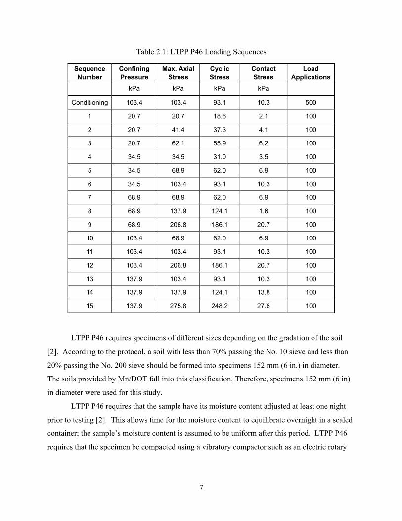
Table 2.1: LTPP P46 Loading Sequences
LTPP P46 requires specimens of different sizes depending on the gradation of the soil
[2]. According to the protocol, a soil with less than 70% passing the No. 10 sieve and less than
20% passing the No. 200 sieve should be formed into specimens 152 mm (6 in.) in diameter.
The soils provided by Mn/DOT fall into this classification. Therefore, specimens 152 mm (6 in)
in diameter were used for this study.
LTPP P46 requires that the sample have its moisture content adjusted at least one night
prior to testing [2]. This allows time for the moisture content to equilibrate overnight in a sealed
container; the sample’s moisture content is assumed to be uniform after this period. LTPP P46
requires that the specimen be compacted using a vibratory compactor such as an electric rotary
Sequence Confining Max. Axial Cyclic Contact Load Number Pressure Stress Stress Stress Applications
kPa kPa kPa kPa
Conditioning 103.4 103.4 93.1 10.3 500
1 20.7 20.7 18.6 2.1 100
2 20.7 41.4 37.3 4.1 100
3 20.7 62.1 55.9 6.2 100
4 34.5 34.5 31.0 3.5 100
5 34.5 68.9 62.0 6.9 100
6 34.5 103.4 93.1 10.3 100
7 68.9 68.9 62.0 6.9 100
8 68.9 137.9 124.1 1.6 100
9 68.9 206.8 186.1 20.7 100
10 103.4 68.9 62.0 6.9 100
11 103.4 103.4 93.1 10.3 100
12 103.4 206.8 186.1 20.7 100
13 137.9 103.4 93.1 10.3 100
14 137.9 137.9 124.1 13.8 100
15 137.9 275.8 248.2 27.6 100

8
or demolition hammer. In addition, the specimen must be compacted in six 51 mm (2 in.) lifts to
create a specimen 305 mm (12 in.) in height.
The lifts are compacted by the compactive effort of the rotary hammer acting on a
compaction plate set on the surface of the sample within the mold; the purpose of the compaction
plate is to spread the force evenly over the surface of the specimen. LTPP P46 requires that
compaction plates be at least 13 mm (0.5 in.) in thickness and 146 mm (5.75 in.) in diameter to
prevent soil from escaping around its edges. Following the compaction of each lift, LTPP P46
requires that the density of the specimen be calculated. Lastly, the specimen is moved to the
load frame to undergo the loading sequences detailed in Table 2.1.
2.1.2 Equipment Modifications
LTPP P46 sets forth several requirements for MR specimen preparation. However, the protocol
leaves room for technicians to improve upon the standard triaxial apparatus if a superior option is
available. As a result, many MR testing laboratories have made adjustments to the triaxial cell
and load frame that they believe to be beneficial. In particular, many researchers have proposed
improvements to the specimen deformation measurement procedure. LTPP P46 requires no
more than two linear variable differential transformers (LVDTs) measuring the displacement of
the load shaft relative to the top cap on the exterior of the cell. However, Tatsuoka et al. [6]
recommend measuring displacement values locally. They found that LVDT measurements on
the exterior of the cell often overestimated the displacement within the specimen due to bedding
errors near the platens. Furthermore, they found that this measurement error was noticeable
during both cyclic and static testing for a wide range of strains. These findings, as well as
similar reports from other researchers, prompted the development of systems designed to
measure the specimens’ deformations locally by fixing three LVDTs to the surface of the
specimen.
Cuccivillo and Coop [7] note that the verticality of the LVDTs may be difficult to
guarantee using this arrangement; the orientation of the LVDTs may be affected by specimen
barreling, tilting, and plastic deformations. However, Cuccivillo and Coop point out that the
error produced by tilted LVDTs is relatively small; a relatively large 8° angle between an LVDT
and a specimen would reduce the LVDT’s axial displacement reading by only 1%. In most

9
specimens, any LVDT tilting that occurs will have a far smaller angle and, therefore, its affect on
the axial displacement reading will often be negligible.
LTPP P46 does not require that the load cell be placed in any particular location relative
to the specimen and chamber as long as the axial force is measured directly. However, it is
considered good practice to place the load cell inside of the pressure vessel. An interior
placement ensures that any affects from the friction produced along the load shaft will not appear
in the load data. Also, when placing the load cell internally there are fewer interfaces between
the load cell and specimen within which similar problems may develop.
It is often recommended that the aggregate present in a soil specimen be no larger than
10% of the specimen’s diameter. Triaxial testing is based on the assumption that the specimen is
relatively uniform; aggregate larger than 10% of the specimen’s diameter is too large for this
assumption to be valid. Therefore, it is recommended that all aggregate over this threshold be
removed from samples prior to specimen preparation.
2.2 Bender Element Testing
Bender elements are short, piezoelectric cantilever strips that contact a specimen. Motion is
triggered in the piezoelectric material by sending an electrical pulse to one of the elements; this
ultimately produces compressional (P) or shear (S) waves in the soil depending upon the
orientation of the piezoelectric material (Figure 2.2).
Figure 2.2: Bender Element Wave Generation
S-wave source
P-wave source

10
The wave produced by the element propagates through the specimen and induces a
voltage in a second bender element located on an opposing surface. A number of quantities,
including small strain modulus values, can be calculated by recording the time histories of these
waves. This calculation procedure is contained in section 4.3.
2.2.1 Density Effects
The small strain shear modulus is calculated using:
2
scG ρ= (2.1)
where G is the shear modulus, ρ is the density, and cs is the shear wave speed. Therefore, the
density of the soil is an important quantity and it should be carefully monitored throughout MR
testing to ascertain that the correct value of ρ is used for the time at which the bender element
test is performed.
The density variation produced by cyclic loading and changes in confinement influence
the value of G. The density of a specimen is difficult to measure after being sealed in a chamber.
Therefore, only the initial value of density is readily available for use in equation (2.1). The
assumption must be made that the change in density over the course of the test is negligible.
Jovicic and Coop [8] studied the effects of confining pressure on the density of three different
sandy soils by steadily increasing confinement to 138 kPa (20 psi), which is the maximum value
of confining pressure in LTPP P46, while periodically taking measurements. Jovicic and Coop
observed increases in density of up to 2% over this range. However, Jovicic and Coop were
quick to note that the average density increase was closer to 1% and that this amount of error is
often negligible in soil testing.
A second cause of density increases in triaxial testing is the applied loading. The only
method by which changes in specimen density due to loading can be measured is by calculating
the density of a specimen before and after testing. This often proves difficult because
accumulated plastic deformations typically cause specimen barreling, which makes it difficult to
model the volume of the specimen. Limited measurements performed for this study indicated
that the density increase was no more than 2% due to the applied loading.

11
2.2.2 Wave Speed Effects
A second variable that affects the calculation of G is the shear wave speed, which is squared in
equation (2.1). As a result, G is more sensitive to variation in the wave speed of a specimen than
it is to variation in its density. Small variations in the shear wave speed that are not the result of
variation in a material’s modulus have the potential to introduce significant error into the
calculation of G. Therefore, it is important to identify potential sources of this error.
One variable that affects the shear wave speed in a soil is the strain level induced by the
shear wave. The stress-strain curve is assumed to be linear at small strain values; G is at its
maximum value in this region (GMAX). However, if the shear strain passes the elastic limit, G
begins to deviate from GMAX. Atkinson and Sallfors [4] suggest that the strain level dividing the
elastic and elastoplastic regions of the stress-strain plot, known as the elastic limit, is 0.001% for
sandy soils. Figure 1.1 shows examples of modulus behavior within differing regions of the
stress-strain plot. Lai and Rix [5] agree that 0.001% is an accurate estimate of the elastic limit
for sands. However, they note that the elastic limit for fine-grained materials is an order of
magnitude or larger. Fortunately, bender elements produce shear strains significantly below the
0.001% elastic limit suggested by the literature. As a result, the assumption that bender elements
measure G within the linear portion of the stress-strain curve (GMAX) should be reasonable
regardless of a soil’s composition.
Another variable that may affect the calculation of G is the strain rate of the test. Iwasaki
et al. [9] and Bolton and Wilson [10] demonstrated that there was a strong correspondence
between sand specimens’ dynamic and continuous static loading stiffnesses by comparing the
results from resonant and torsional shear tests. They concluded that the value of G is not rate
dependent for sands. However, Jovicic and Coop [8] point out that there are no displacement
transducers capable of accurately measuring the strains produced by bender elements. They state
that GMAX may be sensitive to the shear strain rate for these strain levels.

12
2.2.3 Research Recommendations
A number of other issues merit consideration while performing bender element tests during a
cyclic triaxial test. To begin with, the effects of the load pulses, dither, and electrical noise of the
load frame on the bender element system are largely unknown. Therefore, Jovicic and Coop [11]
recommend performing bender element measurements during periods in which the specimen is
not being loaded axially. They also recommend powering down all nearby equipment to prevent
it from affecting the data; this includes the load frame and other instrumentation.
In separate studies, Jovicic and Coop [12] and Schmertmann [13] found that periods of
rest between bender element tests may induce volumetric creep due to the confining pressure and
aging processes within the specimen. The apparent aging of the specimen results in a small
increase in GMAX with no measurable volumetric change. Jovicic and Coop found that sand
specimens are particularly vulnerable to these time-dependent processes; one specimen
underwent a 10% increase in GMAX after being allowed to rest for one hour between tests.
Furthermore, they noted that this effect was proportionally worse for specimens being tested at
lower stress levels and for specimens undergoing their first loading. LTPP P46 does not require
any significant pauses between testing sequences [2]. However, small amounts of volumetric
creep may occur simply due to the length of the MR test, which lasts more than one hour.

13
Chapter 3 Test Procedure
LTPP P46 has specific requirements regarding the instrumentation used to test the resilient
modulus values of a soil [2]. In addition, this study requires that several modifications be made
to the standard resilient modulus test system. The load cell and LVDT instrumentation must be
capable of accurately measuring the load and displacement values produced during the protocol’s
loading sequences. The load frame must be large enough to accommodate the cell, be capable of
producing the forces required in the protocol, and have a known phase angle. The triaxial cell
must be capable of accommodating cylindrical specimens 152 mm (6 in.) in diameter with
functioning bender elements mounted inside its platens. In addition, this cell must be able to
allow the load cell and LVDTs to work while in contact with the specimen. The components of
this test system, the composition of the soil samples, and the test procedure followed during this
study will be discussed. A step-by-step list of the test procedure is included in Appendix E.
3.1 Test Equipment
A large variety of equipment was necessary to perform the testing desired for this study. A
bender element system was purchased and incorporated into triaxial platens. A triaxial cell
meeting the requirements of both LTPP P46 and the bender element instrumentation was
designed and manufactured. Load cell and LVDT instrumentation were purchased and
incorporated into the cell. The design and use of this equipment is contained in this section.
3.1.1 Triaxial Cell
The first objective of this study was to create a triaxial cell that meets the requirements of LTPP
P46, the bender element system, and the internal instrumentation. LTPP P46 requires that the
triaxial cell be large enough to contain a cylindrical specimen 305 mm (12 in.) in height and 152
mm (6 in.) in diameter that can withstand internal pressures of at least 170 kPa (25 psi). The
bender element system requires upper platens at least 30 mm (1.2 in.) in thickness as well as two

14
pressure feedthroughs for its cords. The load cell requires 60 mm (2.4 in.) of open space above
the specimen, and the LVDT apparatus requires at least 13 mm (0.5 in.) of open space around the
specimen’s diameter.
A triaxial cell meeting these specifications was purchased from Research Engineering
(Grass Valley, CA); Figure 3.1 is a diagram of this cell.
Figure 3.1: Triaxial Cell Diagram
Base Plate
Porous Stone with Bender Element Hole
Chamber Wall
Lower Platen
Upper PlatenLoad Cell
Ball Bearing
Top Cap
Load Shaft
305 mm
152 mm
20 mm
241 mm
495 mm
Fluid Ports ( Electrical Feedthroughs on Back)
Support Column
15
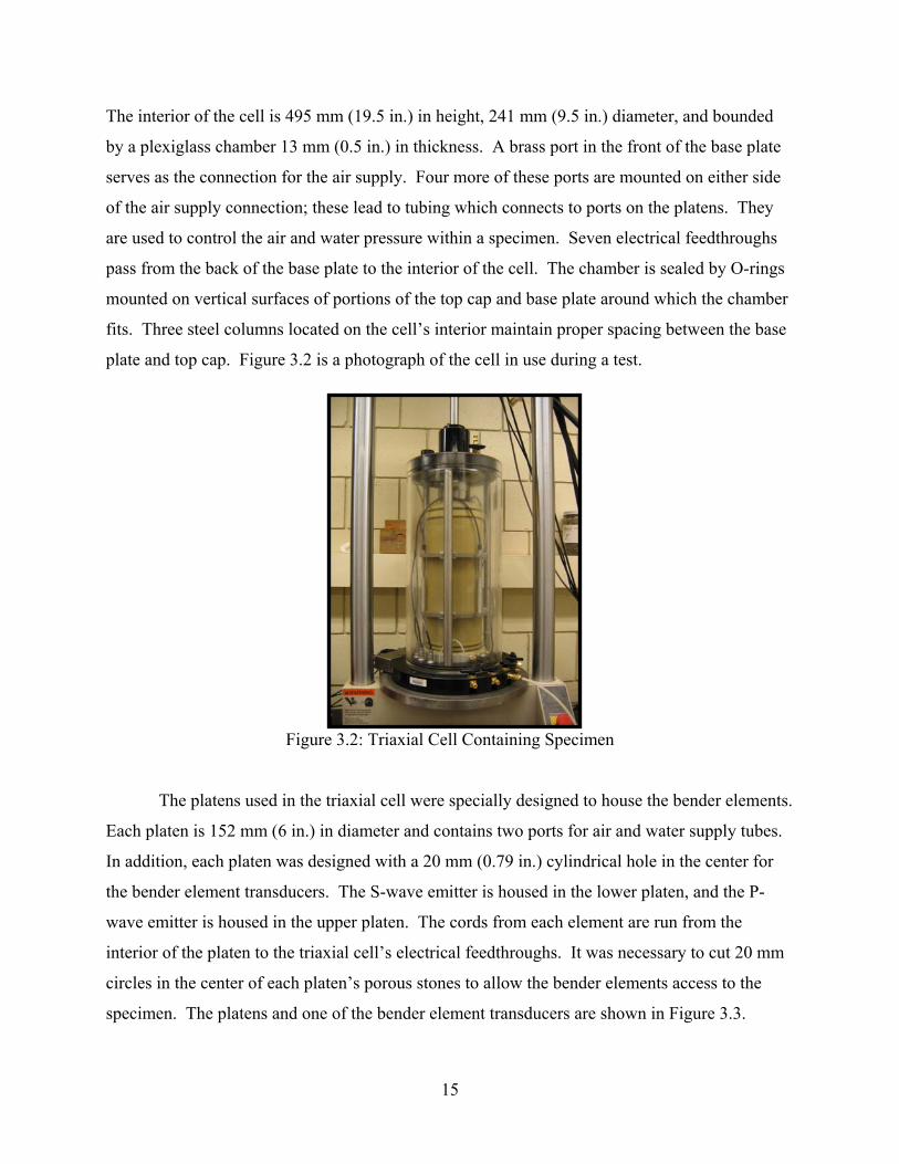
The interior of the cell is 495 mm (19.5 in.) in height, 241 mm (9.5 in.) diameter, and bounded
by a plexiglass chamber 13 mm (0.5 in.) in thickness. A brass port in the front of the base plate
serves as the connection for the air supply. Four more of these ports are mounted on either side
of the air supply connection; these lead to tubing which connects to ports on the platens. They
are used to control the air and water pressure within a specimen. Seven electrical feedthroughs
pass from the back of the base plate to the interior of the cell. The chamber is sealed by O-rings
mounted on vertical surfaces of portions of the top cap and base plate around which the chamber
fits. Three steel columns located on the cell’s interior maintain proper spacing between the base
plate and top cap. Figure 3.2 is a photograph of the cell in use during a test.
Figure 3.2: Triaxial Cell Containing Specimen
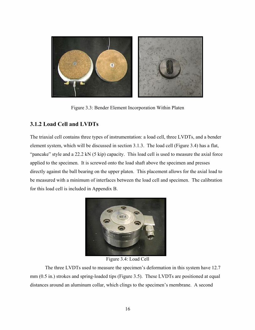
The platens used in the triaxial cell were specially designed to house the bender elements.
Each platen is 152 mm (6 in.) in diameter and contains two ports for air and water supply tubes.
In addition, each platen was designed with a 20 mm (0.79 in.) cylindrical hole in the center for
the bender element transducers. The S-wave emitter is housed in the lower platen, and the P-
wave emitter is housed in the upper platen. The cords from each element are run from the
interior of the platen to the triaxial cell’s electrical feedthroughs. It was necessary to cut 20 mm
circles in the center of each platen’s porous stones to allow the bender elements access to the
specimen. The platens and one of the bender element transducers are shown in Figure 3.3.
16
Figure 3.3: Bender Element Incorporation Within Platen
3.1.2 Load Cell and LVDTs
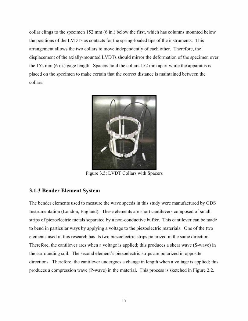
The triaxial cell contains three types of instrumentation: a load cell, three LVDTs, and a bender
element system, which will be discussed in section 3.1.3. The load cell (Figure 3.4) has a flat,
“pancake” style and a 22.2 kN (5 kip) capacity. This load cell is used to measure the axial force
applied to the specimen. It is screwed onto the load shaft above the specimen and presses
directly against the ball bearing on the upper platen. This placement allows for the axial load to
be measured with a minimum of interfaces between the load cell and specimen. The calibration
for this load cell is included in Appendix B.
Figure 3.4: Load Cell
The three LVDTs used to measure the specimen’s deformation in this system have 12.7
mm (0.5 in.) strokes and spring-loaded tips (Figure 3.5). These LVDTs are positioned at equal
distances around an aluminum collar, which clings to the specimen’s membrane. A second
17
collar clings to the specimen 152 mm (6 in.) below the first, which has columns mounted below
the positions of the LVDTs as contacts for the spring-loaded tips of the instruments. This
arrangement allows the two collars to move independently of each other. Therefore, the
displacement of the axially-mounted LVDTs should mirror the deformation of the specimen over
the 152 mm (6 in.) gage length. Spacers hold the collars 152 mm apart while the apparatus is
placed on the specimen to make certain that the correct distance is maintained between the
collars.
Figure 3.5: LVDT Collars with Spacers
3.1.3 Bender Element System
The bender elements used to measure the wave speeds in this study were manufactured by GDS
Instrumentation (London, England). These elements are short cantilevers composed of small
strips of piezoelectric metals separated by a non-conductive buffer. This cantilever can be made
to bend in particular ways by applying a voltage to the piezoelectric materials. One of the two
elements used in this research has its two piezoelectric strips polarized in the same direction.
Therefore, the cantilever arcs when a voltage is applied; this produces a shear wave (S-wave) in
the surrounding soil. The second element’s piezoelectric strips are polarized in opposite
directions. Therefore, the cantilever undergoes a change in length when a voltage is applied; this
produces a compression wave (P-wave) in the material. This process is sketched in Figure 2.2.

18
The bender elements manufactured by GDS Instrumentation are designed to be used as
inserts for the platens bounding a triaxial specimen. A wave produced by one of these elements
travels through the soil specimen and causes the opposing element’s cantilever to deflect; the
history of the voltage that this induces is a record of the received waveform. Therefore, the
element that emits S-waves also receives P-waves. Likewise, the element that emits P-waves
receives S-waves. A photograph of an element mounted within one of the porous stones is
included as Figure 3.6.
Figure 3.6: Bender Element Cantilever Strip
The bender elements are controlled by the Bender Element System (GDS-BES) program.
It is possible to change the frequency, amplitude, and time history of the electrical pulse applied
to the elements using this program. The testing performed in this study makes use of a 5,000 Hz
haversine pulse for P-waves and 2,000 Hz pulse for S-waves. It was demonstrated in section
2.2.2 that the frequency of the pulse does not significantly affect the wave speed over this range.
Therefore, the 5,000 and 2,000 Hz values were used because they tend to induce the cleanest
initial deflections within the received traces. The waves were emitted using the largest
amplitude available within the system, 14 V, so that the signal can be distinguished from
environmental noise.

19
3.1.4 Load Frame
The servo-hydraulic load frame (MTS Systems, Eden Prairie, MN) has a maximum capacity of
22.2 kN (5 kips) and a maximum stroke of 102 mm (4 in.). This frame’s actuator is mounted in a
crossbeam capable of being raised and lowered to accommodate cells of different sizes, which
rest on a steel plate at the base of the frame. The system is operated using a digital controller
named MTS TestStar.
The delay between the load and displacement histories caused by this frame was
calculated to be 0.014 ms using the procedure recommended by LTPP P46. This results in a
phase angle of 0.25°. The complete phase angle data for each LVDT are contained in Appendix
B.1. A photograph of the load frame is included as Figure 3.7.
Figure 3.7: Load Frame
3.2 Soil Samples
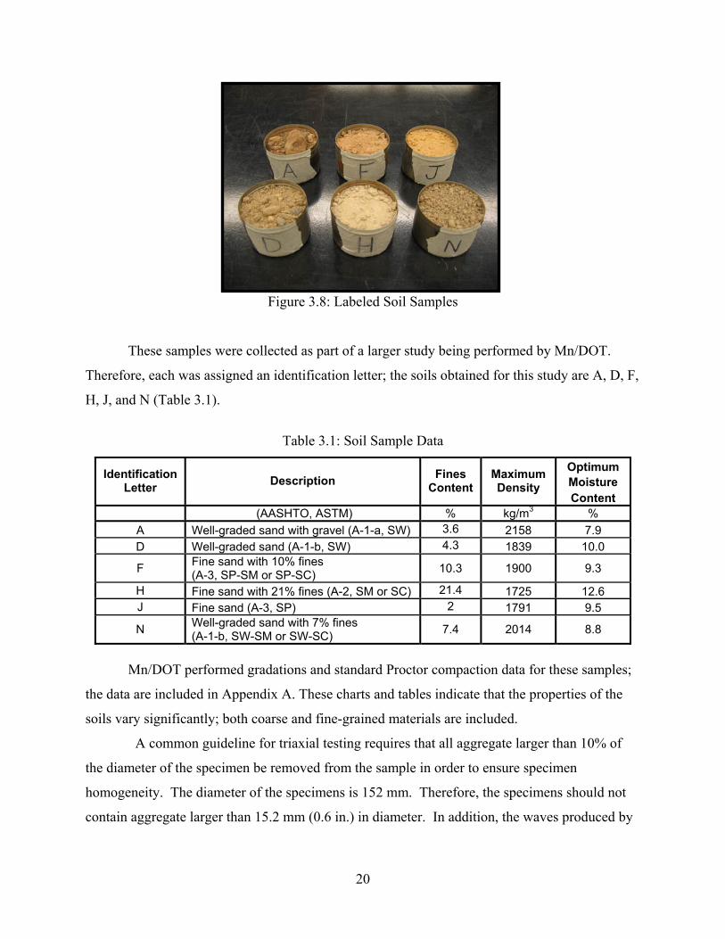
Mn/DOT provided six soil samples for use in this study (Figure 3.8). These samples were
selected to represent the range of granular materials that would be classified as “selected granular
or granular” subbase in pavement structures throughout Minnesota.
20
Figure 3.8: Labeled Soil Samples
These samples were collected as part of a larger study being performed by Mn/DOT.
Therefore, each was assigned an identification letter; the soils obtained for this study are A, D, F,
H, J, and N (Table 3.1).
Table 3.1: Soil Sample Data
Optimum Moisture Identification
Letter Description Fines Content
Maximum Density
Content (AASHTO, ASTM) % kg/m3 % A Well-graded sand with gravel (A-1-a, SW) 3.6 2158 7.9 D Well-graded sand (A-1-b, SW) 4.3 1839 10.0
F Fine sand with 10% fines (A-3, SP-SM or SP-SC) 10.3 1900 9.3
H Fine sand with 21% fines (A-2, SM or SC) 21.4 1725 12.6 J Fine sand (A-3, SP) 2 1791 9.5
N Well-graded sand with 7% fines (A-1-b, SW-SM or SW-SC) 7.4 2014 8.8
Mn/DOT performed gradations and standard Proctor compaction data for these samples;
the data are included in Appendix A. These charts and tables indicate that the properties of the
soils vary significantly; both coarse and fine-grained materials are included.
A common guideline for triaxial testing requires that all aggregate larger than 10% of
the diameter of the specimen be removed from the sample in order to ensure specimen
homogeneity. The diameter of the specimens is 152 mm. Therefore, the specimens should not
contain aggregate larger than 15.2 mm (0.6 in.) in diameter. In addition, the waves produced by
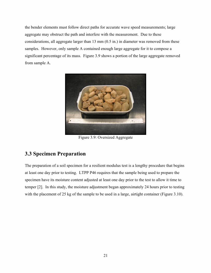
21
the bender elements must follow direct paths for accurate wave speed measurements; large
aggregate may obstruct the path and interfere with the measurement. Due to these
considerations, all aggregate larger than 13 mm (0.5 in.) in diameter was removed from these
samples. However, only sample A contained enough large aggregate for it to compose a
significant percentage of its mass. Figure 3.9 shows a portion of the large aggregate removed
from sample A.
Figure 3.9: Oversized Aggregate
3.3 Specimen Preparation
The preparation of a soil specimen for a resilient modulus test is a lengthy procedure that begins
at least one day prior to testing. LTPP P46 requires that the sample being used to prepare the
specimen have its moisture content adjusted at least one day prior to the test to allow it time to
temper [2]. In this study, the moisture adjustment began approximately 24 hours prior to testing
with the placement of 25 kg of the sample to be used in a large, airtight container (Figure 3.10).

22
Figure 3.10: Tempering Container
The amount of water necessary to bring the sample to the target moisture content was
calculated using:
−
=100
1ωωWWaw (3.1)
where Waw is the weight of water to add, W is the weight of the sample, ω is the desired moisture
content, and ω1 is the current moisture content. This water was added to the sample by
sprinkling small amounts over its entire surface while mixing thoroughly. After adding the
water, three moisture content samples were taken from several different locations within the
container and placed in an oven overnight at 52° C (125° F). The container was then sealed and
the soil’s moisture content was left to equilibrate.
The following day the moisture contents samples were removed from the oven and the
sample’s moisture content was calculated. If the moisture content of the sample was within
0.5% of the desired moisture content, then the sample was prepared for compaction. If the
measured moisture content was outside of the acceptable range, however, it was necessary to
make a second adjustment. Additional water or dry soil was added until the correct moisture
content was achieved.
23
3.3.1 Compaction
LTPP P46 requires that specimens be compacted in six lifts using vibratory compaction [2]. This
compaction took place on a countertop near the load frame. The rubber membrane used to
surround the specimen was slid over the bottom platen and porous stone and sealed with two O-
rings. The vacuum mold was placed on top of the platen and sealed with two ring clamps. The
upper clamp was placed over the portion of the membrane emerging from the vacuum mold to
hold it in place. A 30 kPa (4.2 psi) vacuum was applied.
Before compacting the soil, it was necessary to protect the lower platen’s bender element
from large aggregate by covering it with a small amount of fine sand (Ottawa 50-70). The
rationale behind this protection is discussed in section 3.3.3. After adding the buffer sand the
entire mold was weighed.
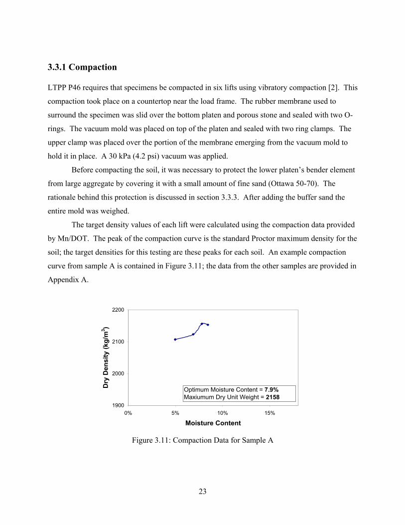
The target density values of each lift were calculated using the compaction data provided
by Mn/DOT. The peak of the compaction curve is the standard Proctor maximum density for the
soil; the target densities for this testing are these peaks for each soil. An example compaction
curve from sample A is contained in Figure 3.11; the data from the other samples are provided in
Appendix A.
1900
2000
2100
2200
0% 5% 10% 15%
Moisture Content
Dry
Den
sity
(kg/
m3 )
Optimum Moisture Content = 7.9%Maxiumum Dry Unit Weight = 2158
Figure 3.11: Compaction Data for Sample A
24
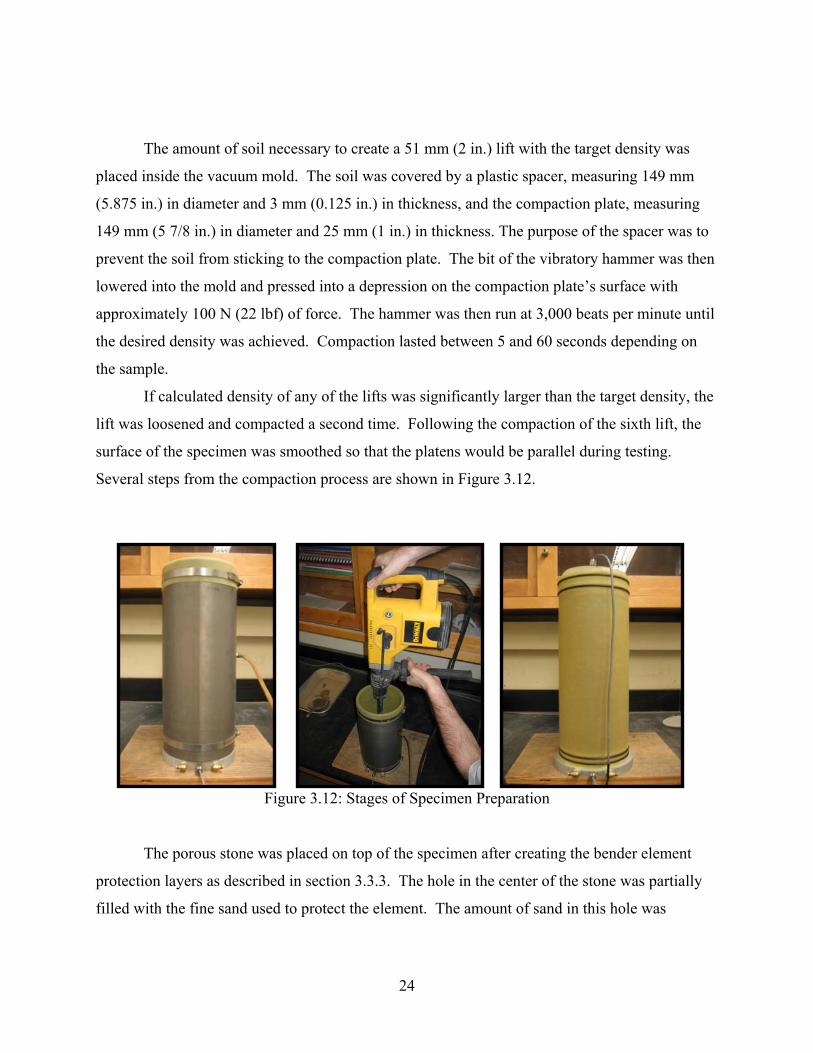
The amount of soil necessary to create a 51 mm (2 in.) lift with the target density was
placed inside the vacuum mold. The soil was covered by a plastic spacer, measuring 149 mm
(5.875 in.) in diameter and 3 mm (0.125 in.) in thickness, and the compaction plate, measuring
149 mm (5 7/8 in.) in diameter and 25 mm (1 in.) in thickness. The purpose of the spacer was to
prevent the soil from sticking to the compaction plate. The bit of the vibratory hammer was then
lowered into the mold and pressed into a depression on the compaction plate’s surface with
approximately 100 N (22 lbf) of force. The hammer was then run at 3,000 beats per minute until
the desired density was achieved. Compaction lasted between 5 and 60 seconds depending on
the sample.
If calculated density of any of the lifts was significantly larger than the target density, the
lift was loosened and compacted a second time. Following the compaction of the sixth lift, the
surface of the specimen was smoothed so that the platens would be parallel during testing.
Several steps from the compaction process are shown in Figure 3.12.
Figure 3.12: Stages of Specimen Preparation
The porous stone was placed on top of the specimen after creating the bender element
protection layers as described in section 3.3.3. The hole in the center of the stone was partially
filled with the fine sand used to protect the element. The amount of sand in this hole was
25
adjusted until the transducer and platen sat on top of it evenly and it could be seen that the
transducer was pressing into the soil. O-rings were used to seal the membrane and the vacuum
supply was shut off. All of the specimens prepared contained enough cohesion to hold the
specimens together without confinement.
A second membrane was pulled over the first after removing the split vacuum mold. The
pounding of the rotary hammer caused small tears in some of the specimens’ membranes.
Therefore, it was necessary to make certain that the specimen remained sealed using this
additional membrane. Lastly, O-rings were placed over the surface of the outer membrane to
seal it.
3.3.2 Percometer Measurements
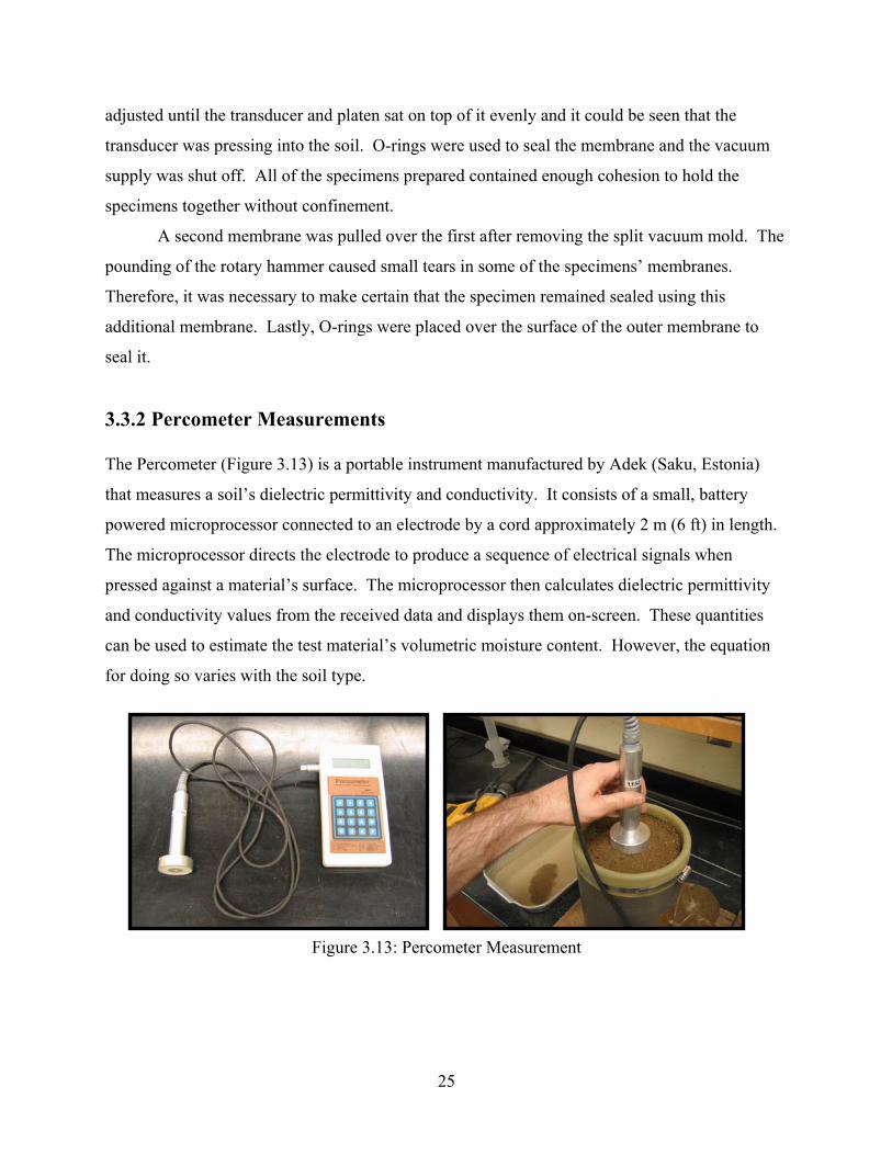
The Percometer (Figure 3.13) is a portable instrument manufactured by Adek (Saku, Estonia)
that measures a soil’s dielectric permittivity and conductivity. It consists of a small, battery
powered microprocessor connected to an electrode by a cord approximately 2 m (6 ft) in length.
The microprocessor directs the electrode to produce a sequence of electrical signals when
pressed against a material’s surface. The microprocessor then calculates dielectric permittivity
and conductivity values from the received data and displays them on-screen. These quantities
can be used to estimate the test material’s volumetric moisture content. However, the equation
for doing so varies with the soil type.
Figure 3.13: Percometer Measurement
26
In this study, the Percometer was used on the surface of the specimen following
compaction. Three measurements were taken across a diameter of the compacted specimen in
order to account for any edge effects from the aluminum split mold.
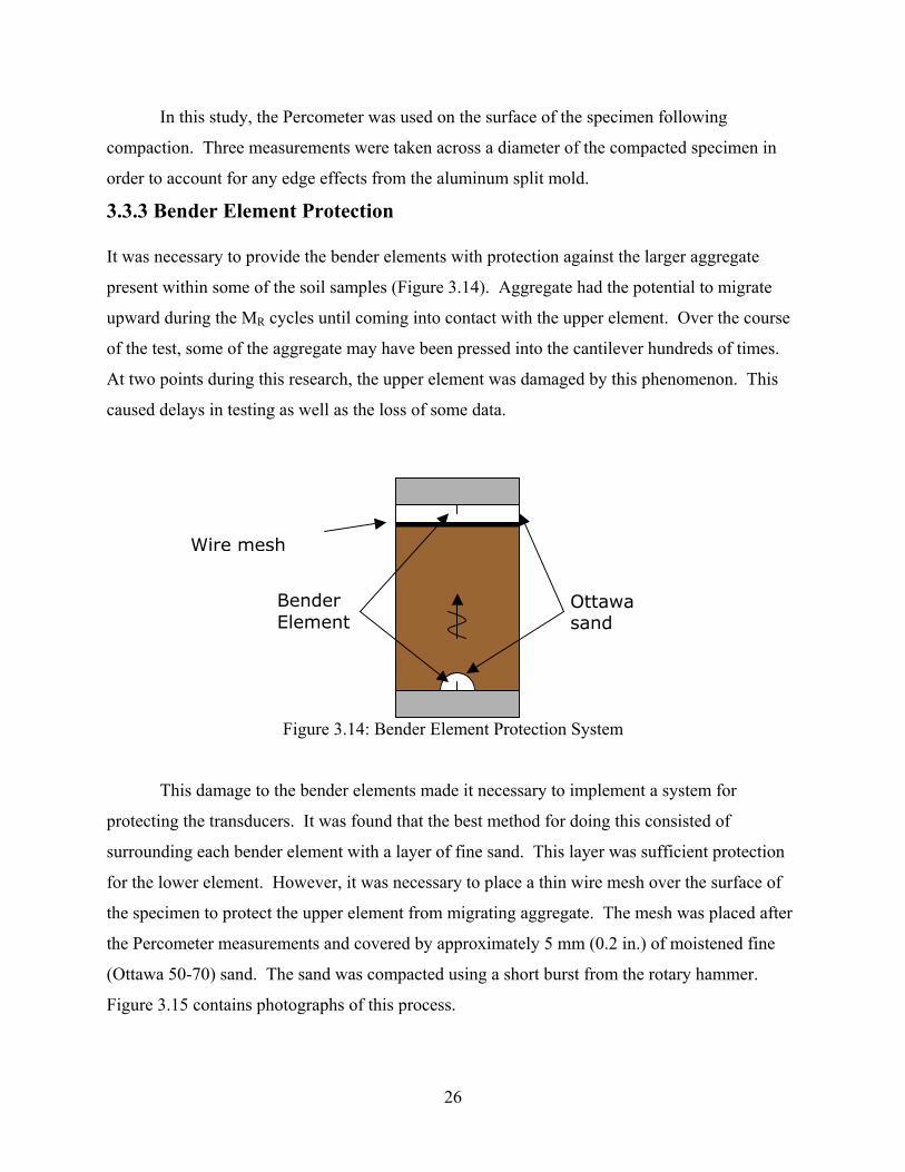
3.3.3 Bender Element Protection
It was necessary to provide the bender elements with protection against the larger aggregate
present within some of the soil samples (Figure 3.14). Aggregate had the potential to migrate
upward during the MR cycles until coming into contact with the upper element. Over the course
of the test, some of the aggregate may have been pressed into the cantilever hundreds of times.
At two points during this research, the upper element was damaged by this phenomenon. This
caused delays in testing as well as the loss of some data.
Figure 3.14: Bender Element Protection System
This damage to the bender elements made it necessary to implement a system for
protecting the transducers. It was found that the best method for doing this consisted of
surrounding each bender element with a layer of fine sand. This layer was sufficient protection
for the lower element. However, it was necessary to place a thin wire mesh over the surface of
the specimen to protect the upper element from migrating aggregate. The mesh was placed after
the Percometer measurements and covered by approximately 5 mm (0.2 in.) of moistened fine
(Ottawa 50-70) sand. The sand was compacted using a short burst from the rotary hammer.
Figure 3.15 contains photographs of this process.
Bender Element
Ottawa sand
Wire mesh
27
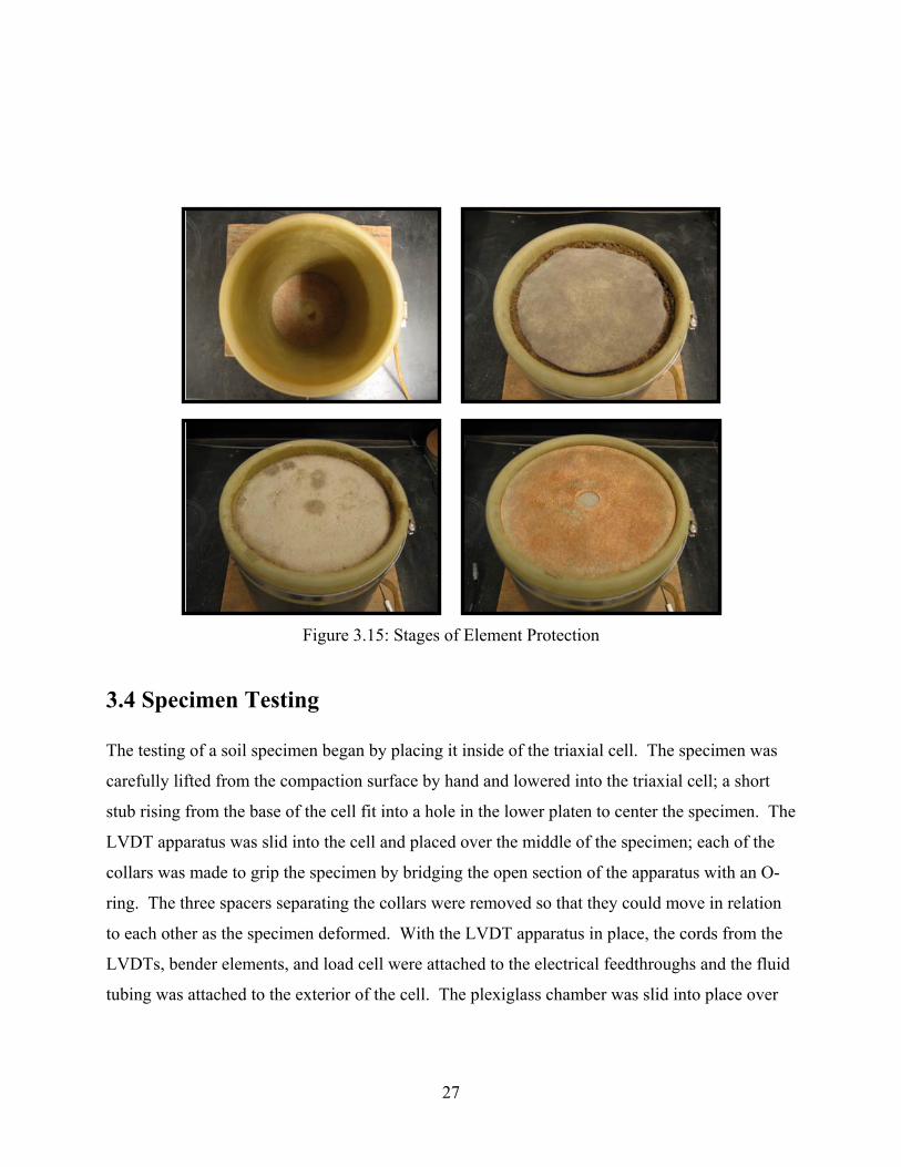
Figure 3.15: Stages of Element Protection
3.4 Specimen Testing
The testing of a soil specimen began by placing it inside of the triaxial cell. The specimen was
carefully lifted from the compaction surface by hand and lowered into the triaxial cell; a short
stub rising from the base of the cell fit into a hole in the lower platen to center the specimen. The
LVDT apparatus was slid into the cell and placed over the middle of the specimen; each of the
collars was made to grip the specimen by bridging the open section of the apparatus with an O-
ring. The three spacers separating the collars were removed so that they could move in relation
to each other as the specimen deformed. With the LVDT apparatus in place, the cords from the
LVDTs, bender elements, and load cell were attached to the electrical feedthroughs and the fluid
tubing was attached to the exterior of the cell. The plexiglass chamber was slid into place over

28
the specimen and supports. Figure 3.16 shows a photograph of the specimen following the
placement of this chamber.
Figure 3.16: Specimen Loaded within Triaxial Cell
The entire triaxial cell was then lifted and slid into the load frame. The cords from the
signal conditioners were attached to the electrical feedthroughs. The triaxial cell’s load shaft,
with the top cap and load cell attached, was screwed onto the load frame’s shaft. The load cell’s
cord was attached and the ball bearing was placed on the top of the upper platen. The top cap
was then lowered into position and held in place using three bolts. Two circular plates on the top
cap were rotated over the top of the chamber to prevent it from sliding upward during the test.
3.4.1 Resilient Modulus Test
The resilient modulus test protocol in this study followed the confining pressure and deviator
stress sequence required by LTPP P46 (Table 2.1). The only modification made to the protocol
for the purposes of this research was the complete removal of the axial load before and after
changes in the cell’s confining pressure; these short rest periods were used to perform the bender
element tests.
The first step in the test protocol was the pressurization of the cell for the conditioning
loading sequence. The confining pressure was manually adjusted by turning a knob on the
29
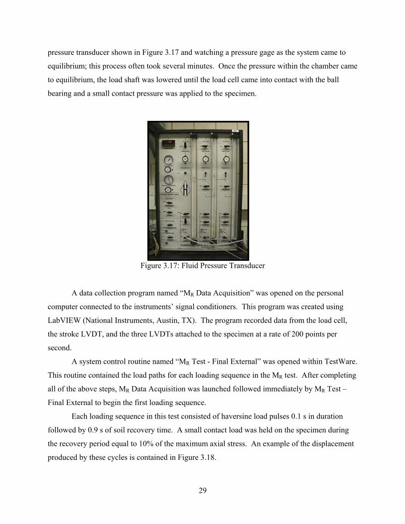
pressure transducer shown in Figure 3.17 and watching a pressure gage as the system came to
equilibrium; this process often took several minutes. Once the pressure within the chamber came
to equilibrium, the load shaft was lowered until the load cell came into contact with the ball
bearing and a small contact pressure was applied to the specimen.
Figure 3.17: Fluid Pressure Transducer
A data collection program named “MR Data Acquisition” was opened on the personal
computer connected to the instruments’ signal conditioners. This program was created using
LabVIEW (National Instruments, Austin, TX). The program recorded data from the load cell,
the stroke LVDT, and the three LVDTs attached to the specimen at a rate of 200 points per
second.
A system control routine named “MR Test - Final External” was opened within TestWare.
This routine contained the load paths for each loading sequence in the MR test. After completing
all of the above steps, MR Data Acquisition was launched followed immediately by MR Test –
Final External to begin the first loading sequence.
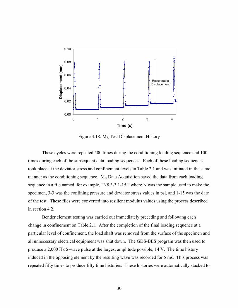
Each loading sequence in this test consisted of haversine load pulses 0.1 s in duration
followed by 0.9 s of soil recovery time. A small contact load was held on the specimen during
the recovery period equal to 10% of the maximum axial stress. An example of the displacement
produced by these cycles is contained in Figure 3.18.
30
0.00
0.02
0.04
0.06
0.08
0.10
0 1 2 3 4
Time (s)
Dis
plac
emen
t (m
m)
Recoverable Displacement
Figure 3.18: MR Test Displacement History
These cycles were repeated 500 times during the conditioning loading sequence and 100
times during each of the subsequent data loading sequences. Each of these loading sequences
took place at the deviator stress and confinement levels in Table 2.1 and was initiated in the same
manner as the conditioning sequence. MR Data Acquisition saved the data from each loading
sequence in a file named, for example, “N8 3-3 1-15,” where N was the sample used to make the
specimen, 3-3 was the confining pressure and deviator stress values in psi, and 1-15 was the date
of the test. These files were converted into resilient modulus values using the process described
in section 4.2.
Bender element testing was carried out immediately preceding and following each
change in confinement on Table 2.1. After the completion of the final loading sequence at a
particular level of confinement, the load shaft was removed from the surface of the specimen and
all unnecessary electrical equipment was shut down. The GDS-BES program was then used to
produce a 2,000 Hz S-wave pulse at the largest amplitude possible, 14 V. The time history
induced in the opposing element by the resulting wave was recorded for 5 ms. This process was
repeated fifty times to produce fifty time histories. These histories were automatically stacked to
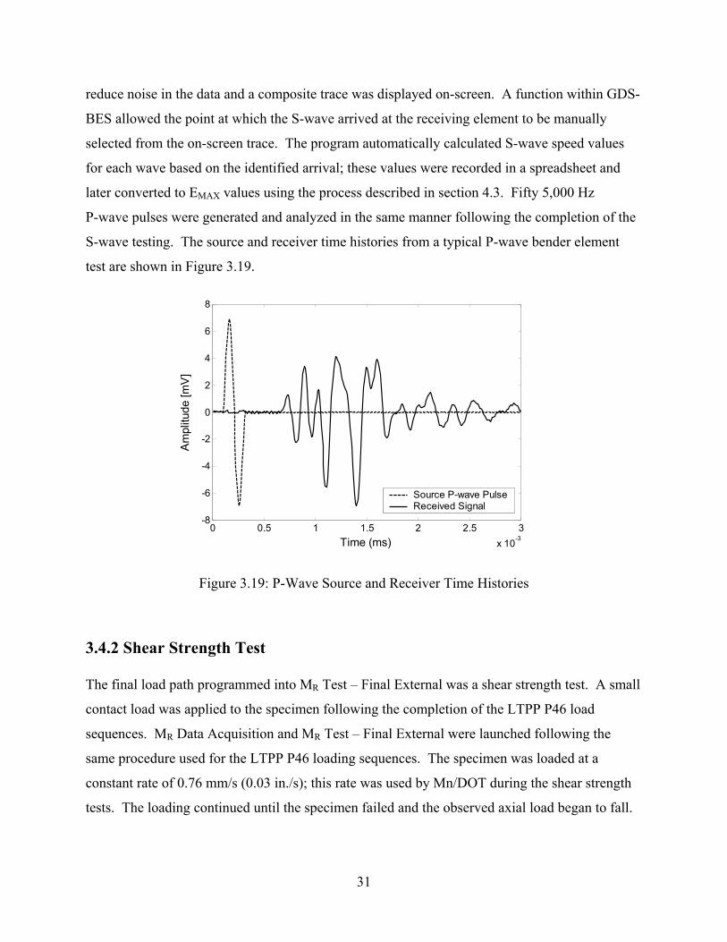
31
reduce noise in the data and a composite trace was displayed on-screen. A function within GDS-
BES allowed the point at which the S-wave arrived at the receiving element to be manually
selected from the on-screen trace. The program automatically calculated S-wave speed values
for each wave based on the identified arrival; these values were recorded in a spreadsheet and
later converted to EMAX values using the process described in section 4.3. Fifty 5,000 Hz
P-wave pulses were generated and analyzed in the same manner following the completion of the
S-wave testing. The source and receiver time histories from a typical P-wave bender element
test are shown in Figure 3.19.
Figure 3.19: P-Wave Source and Receiver Time Histories
3.4.2 Shear Strength Test
The final load path programmed into MR Test – Final External was a shear strength test. A small
contact load was applied to the specimen following the completion of the LTPP P46 load
sequences. MR Data Acquisition and MR Test – Final External were launched following the
same procedure used for the LTPP P46 loading sequences. The specimen was loaded at a
constant rate of 0.76 mm/s (0.03 in./s); this rate was used by Mn/DOT during the shear strength
tests. The loading continued until the specimen failed and the observed axial load began to fall.
0 0.5 1 1.5 2 2.5 3x 10⁻³
-8
-6
-4
-2
0
2
4
6
8
Time (ms)
Am
plitu
de [m
V]
Source P-wave PulseReceived Signal
32
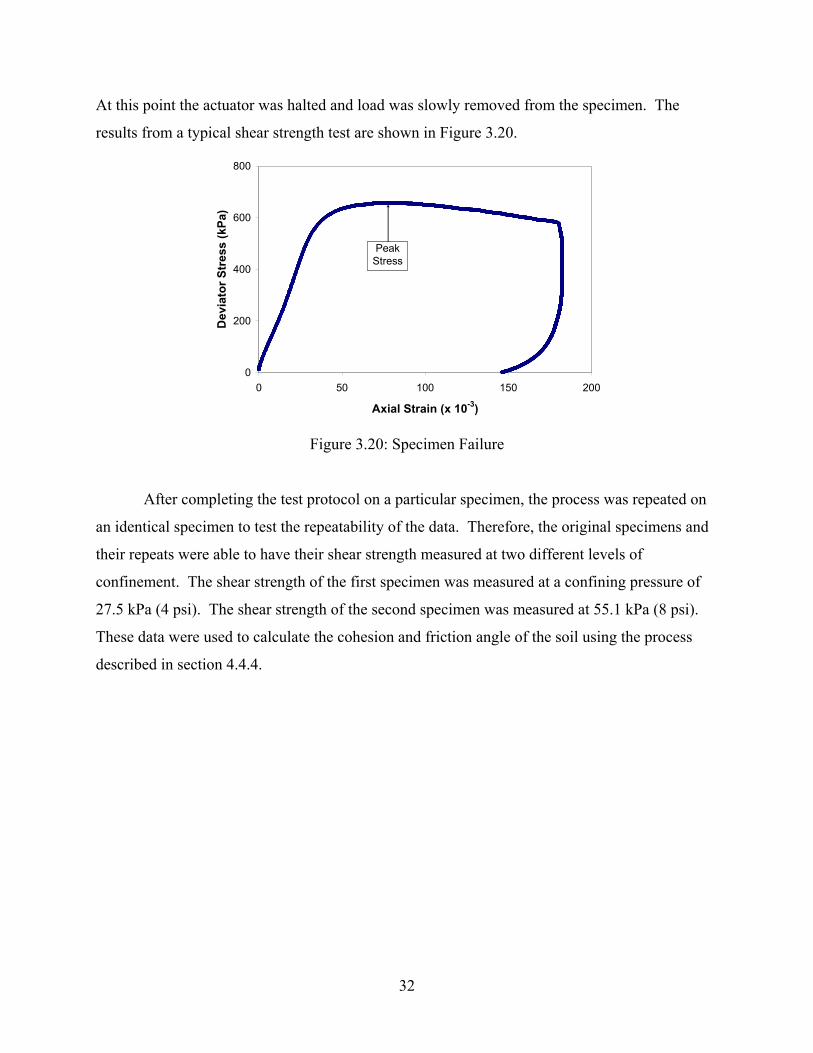
At this point the actuator was halted and load was slowly removed from the specimen. The
results from a typical shear strength test are shown in Figure 3.20.
0
200
400
600
800
0 50 100 150 200
Axial Strain (x 10-3)
Dev
iato
r Str
ess
(kPa
)
PeakStress
Figure 3.20: Specimen Failure
After completing the test protocol on a particular specimen, the process was repeated on
an identical specimen to test the repeatability of the data. Therefore, the original specimens and
their repeats were able to have their shear strength measured at two different levels of
confinement. The shear strength of the first specimen was measured at a confining pressure of
27.5 kPa (4 psi). The shear strength of the second specimen was measured at 55.1 kPa (8 psi).
These data were used to calculate the cohesion and friction angle of the soil using the process
described in section 4.4.4.

33
Chapter 4 Discussion of Results
The six soil samples were tested at three moisture contents at one density using the procedures
described in Chapter 3. The load and displacement data files from the loading sequences were
input into a MATLAB program to calculate resilient modulus values. The wave speeds
measured by the bender elements were used to calculate maximum Young’s modulus values.
The values generated by these procedures were checked for reasonability and repeatability.
Lastly, the hyperbolic model was used to create degradation curves for these data.
4.1 Testing Schedule
Resilient modulus and maximum Young’s modulus values were determined for six soil samples
at three values of moisture content each. These 18 tests were each repeated one time. In total,
the test procedure for this study was performed on 36 different soil specimens.
Mn/DOT provided standard Proctor compaction data for each soil sample so their
optimum moisture content and maximum density values were known. Using these data, it was
decided that the soil samples should be tested at a moisture content near the optimum moisture
content, at a moisture content near the “dry” moisture content of these soils in the field, and at a
value halfway between optimum and “dry”. Soils rarely have moisture contents below
approximately 3% in the field. Therefore, the majority of the “dry” moisture content values were
selected near this value. Each of these samples was compacted to its maximum dry density.
Table 4.1 contains the sample, moisture content, and dry density data for each test.
34
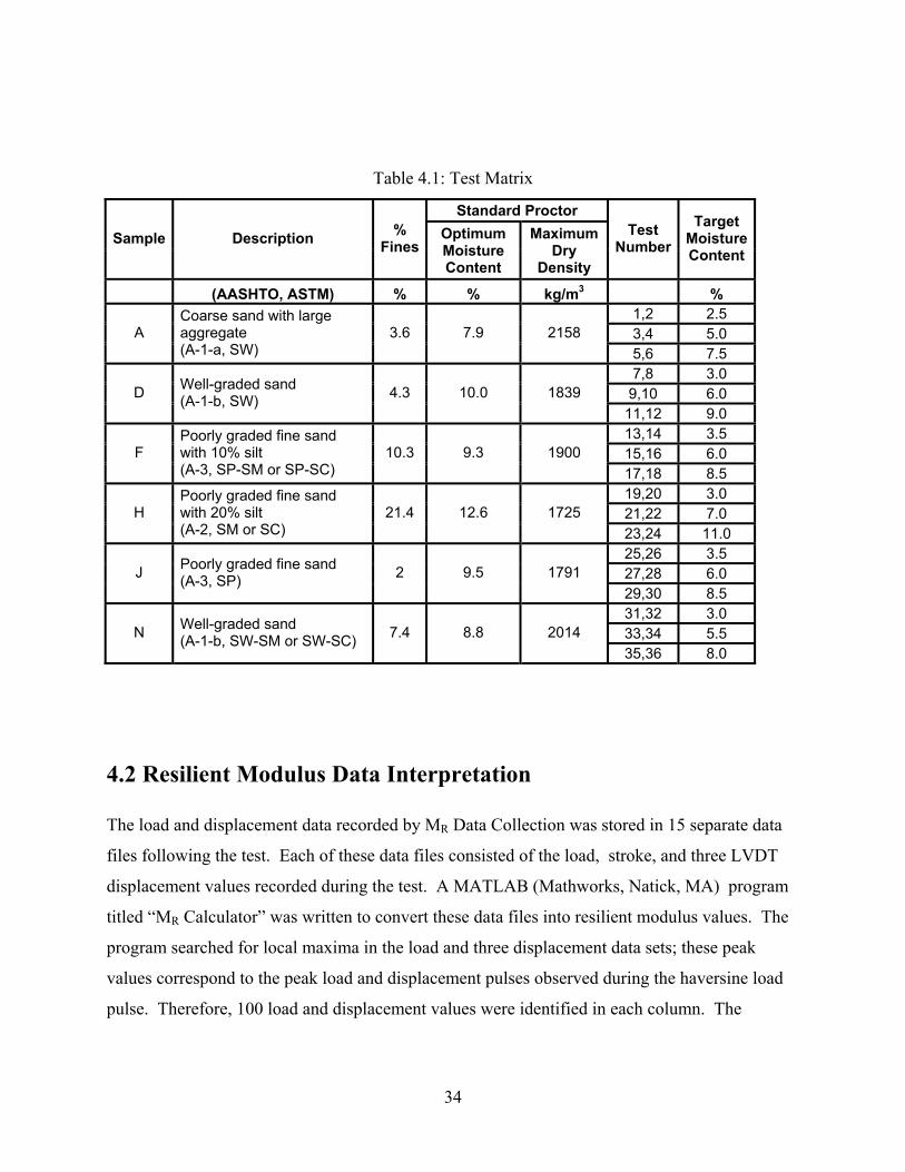
Table 4.1: Test Matrix
Standard Proctor
Sample Description % Fines
Optimum Moisture Content
MaximumDry
Density
Test Number
Target MoistureContent
(AASHTO, ASTM) % % kg/m3 % 1,2 2.5 3,4 5.0 A
Coarse sand with large aggregate (A-1-a, SW)
3.6 7.9 2158 5,6 7.5 7,8 3.0
9,10 6.0 D Well-graded sand (A-1-b, SW) 4.3 10.0 1839
11,12 9.0 13,14 3.5 15,16 6.0 F
Poorly graded fine sand with 10% silt (A-3, SP-SM or SP-SC)
10.3 9.3 1900 17,18 8.5 19,20 3.0 21,22 7.0 H
Poorly graded fine sand with 20% silt (A-2, SM or SC)
21.4 12.6 1725 23,24 11.0 25,26 3.5 27,28 6.0 J Poorly graded fine sand
(A-3, SP) 2 9.5 1791 29,30 8.5 31,32 3.0 33,34 5.5 N Well-graded sand
(A-1-b, SW-SM or SW-SC) 7.4 8.8 2014 35,36 8.0
4.2 Resilient Modulus Data Interpretation
The load and displacement data recorded by MR Data Collection was stored in 15 separate data
files following the test. Each of these data files consisted of the load, stroke, and three LVDT
displacement values recorded during the test. A MATLAB (Mathworks, Natick, MA) program
titled “MR Calculator” was written to convert these data files into resilient modulus values. The
program searched for local maxima in the load and three displacement data sets; these peak
values correspond to the peak load and displacement pulses observed during the haversine load
pulse. Therefore, 100 load and displacement values were identified in each column. The
35
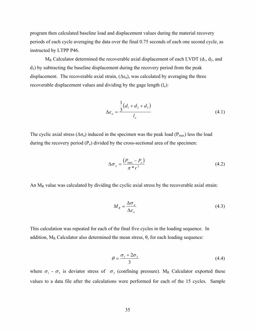
program then calculated baseline load and displacement values during the material recovery
periods of each cycle averaging the data over the final 0.75 seconds of each one second cycle, as
instructed by LTPP P46.
MR Calculator determined the recoverable axial displacement of each LVDT (d1, d2, and
d3) by subtracting the baseline displacement during the recovery period from the peak
displacement. The recoverable axial strain, (∆εa), was calculated by averaging the three
recoverable displacement values and dividing by the gage length (lo):
( )
oa l
ddd 32131
++=∆ε (4.1)
The cyclic axial stress (∆σa) induced in the specimen was the peak load (Pmax) less the load
during the recovery period (Po) divided by the cross-sectional area of the specimen:
( )
2max
* rPP o
a πσ
−=∆ (4.2)
An MR value was calculated by dividing the cyclic axial stress by the recoverable axial strain:
a
aRM
εσ
∆∆
= (4.3)
This calculation was repeated for each of the final five cycles in the loading sequence. In
addition, MR Calculator also determined the mean stress, θ, for each loading sequence:
32 31 σσ
θ+
= (4.4)
where 1σ - 3σ is deviator stress of 3σ (confining pressure). MR Calculator exported these
values to a data file after the calculations were performed for each of the 15 cycles. Sample
36
calculations for this process are contained in section 4.2.1. A copy of the MR Calculator
MATLAB program is contained in Appendix C.
4.2.1 Sample Calculation
The following calculations illustrate the process described in section 4.2 using real data. The
following data comes from cycle 15 of test #24: the repeat of sample H at an 11% moisture
content. The recoverable axial strain for one of the loading sequences was calculated using
equation (4.1). The gage length was 0.1524 m (6 in.).
( ) 3555
10*24.01524.0*3
10*71.310*86.310*58.3 −−−−
=++
=m
mmmaε
The cyclic stress was then calculated using equation (4.2). The radius of the specimen was
0.0762 m (3 in.).
( ) kPam
NNa 3.92
)(0762.0*)(217)(1900
22 =−
=π
σ
The resilient modulus for this cycle was calculated using equation (4.3).
MPakPaM R 37810*24.0
3.923 == −
Lastly, the mean stress was calculated using equation (4.4).
kPakPakPakPa 1733
137137242=
++=θ
4.2.2 Deformation Homogeneity
37
One of the difficulties encountered during this testing was the occasional presence of large
discrepancies between the three LVDT readings. The three displacement histories recorded
during the MR loading sequences were often within 10% of each other. However, there were
also times in which the displacements differed by 100% or more. Several factors may have
contributed to these discrepancies among the three LVDT readings: specimen ends may not have
been parallel, specimens may have tilted or barreled during testing, or there may have been
slippage between the LVDT holder and the membrane.
The LVDT readings were averaged during the calculation of MR so it was difficult to say
what effect, if any, poor LVDT agreement had upon the data. Therefore, it would be beneficial
to identify a homogeneous deformation coefficient, α, to quantify the deformation homogeneity
of the specimens:
d
23
22
21 δδδ
α++
= (4.5)
where δi is the difference between the average LVDT displacement and the displacement from
LVDT ‘i’:
ii dd −=δ (4.6)
and d is the average LVDT displacement:
3321 ddd
d++
= (4.7)
An α-value of 0 indicates perfect LVDT agreement. Larger α-values indicate increasing
discrepancies between the displacement values.
Examples of loading histories with small and large α-values are shown in Figure 4.1. The
loading sequence with the α-value of 1.30 (Figure 4.1b) was from an MR test in which the
specimen began to bend during the load pulses. Every time that a load pulse was applied during
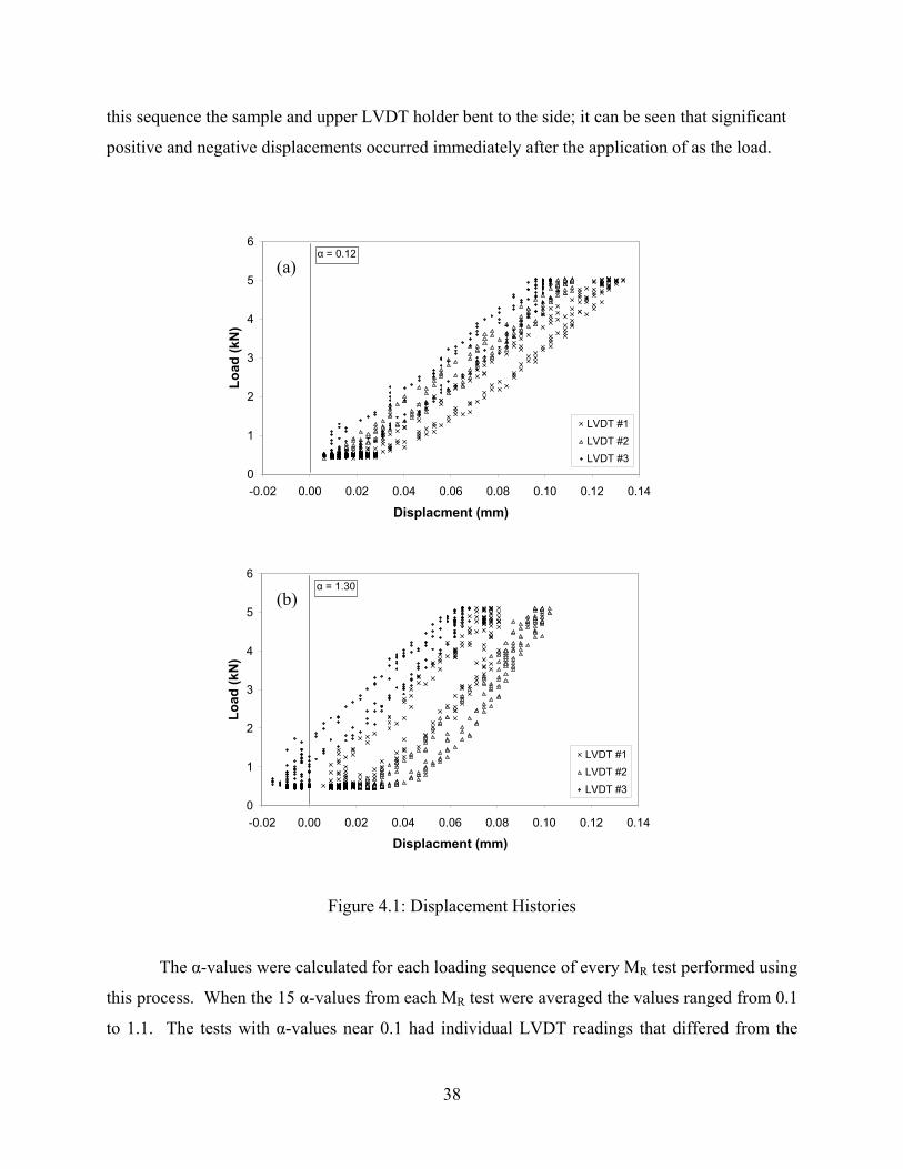
38
this sequence the sample and upper LVDT holder bent to the side; it can be seen that significant
positive and negative displacements occurred immediately after the application of as the load.
Figure 4.1: Displacement Histories
The α-values were calculated for each loading sequence of every MR test performed using
this process. When the 15 α-values from each MR test were averaged the values ranged from 0.1
to 1.1. The tests with α-values near 0.1 had individual LVDT readings that differed from the
0
1
2
3
4
5
6
-0.02 0.00 0.02 0.04 0.06 0.08 0.10 0.12 0.14
Displacment (mm)
Load
(kN
)
LVDT #1LVDT #2LVDT #3
α = 1.30
0
1
2
3
4
5
6
-0.02 0.00 0.02 0.04 0.06 0.08 0.10 0.12 0.14
Displacment (mm)
Load
(kN
)
LVDT #1LVDT #2LVDT #3
α = 0.12(a)
(b)
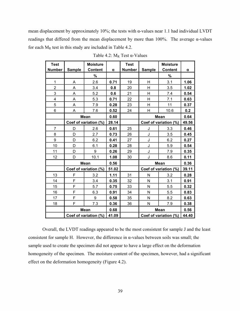
39
mean displacement by approximately 10%; the tests with α-values near 1.1 had individual LVDT
readings that differed from the mean displacement by more than 100%. The average α-values
for each MR test in this study are included in Table 4.2.
Table 4.2: MR Test α-Values
Test Moisture Test Moisture Number Sample Content α Number Sample Content α
% % 1 A 2.6 0.71 19 H 3.1 1.06 2 A 3.4 0.8 20 H 3.5 1.02 3 A 5.2 0.6 21 H 7.4 0.54 4 A 5.3 0.71 22 H 7.1 0.63 5 A 7.9 0.28 23 H 11 0.37 6 A 7.6 0.52 24 H 10.6 0.2 Mean 0.60 Mean 0.64 Coef of variation (%) 28.14 Coef of variation (%) 49.56
7 D 2.6 0.61 25 J 3.3 0.46 8 D 2.7 0.73 26 J 3.5 0.45 9 D 6.2 0.41 27 J 6.2 0.27 10 D 6.1 0.28 28 J 5.9 0.54 11 D 9 0.26 29 J 7.9 0.35 12 D 10.1 1.08 30 J 8.6 0.11
Mean 0.56 Mean 0.36 Coef of variation (%) 51.02 Coef of variation (%) 39.11
13 F 3.2 1.11 31 N 3.2 0.28 14 F 3.4 0.35 32 N 3.1 0.91 15 F 5.7 0.75 33 N 5.5 0.32 16 F 6.3 0.91 34 N 5.5 0.83 17 F 9 0.58 35 N 8.2 0.63 18 F 7.3 0.36 36 N 7.9 0.38
Mean 0.68 Mean 0.56 Coef of variation (%) 41.09 Coef of variation (%) 44.40
Overall, the LVDT readings appeared to be the most consistent for sample J and the least
consistent for sample H. However, the difference in α-values between soils was small; the
sample used to create the specimen did not appear to have a large effect on the deformation
homogeneity of the specimen. The moisture content of the specimen, however, had a significant
effect on the deformation homogeneity (Figure 4.2).
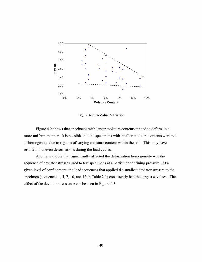
40
Figure 4.2: α-Value Variation
Figure 4.2 shows that specimens with larger moisture contents tended to deform in a
more uniform manner. It is possible that the specimens with smaller moisture contents were not
as homogenous due to regions of varying moisture content within the soil. This may have
resulted in uneven deformations during the load cycles.
Another variable that significantly affected the deformation homogeneity was the
sequence of deviator stresses used to test specimens at a particular confining pressure. At a
given level of confinement, the load sequences that applied the smallest deviator stresses to the
specimen (sequences 1, 4, 7, 10, and 13 in Table 2.1) consistently had the largest α-values. The
effect of the deviator stress on α can be seen in Figure 4.3.
0.00
0.20
0.40
0.60
0.80
1.00
1.20
0% 2% 4% 6% 8% 10% 12%
Moisture Content
α-V
alue
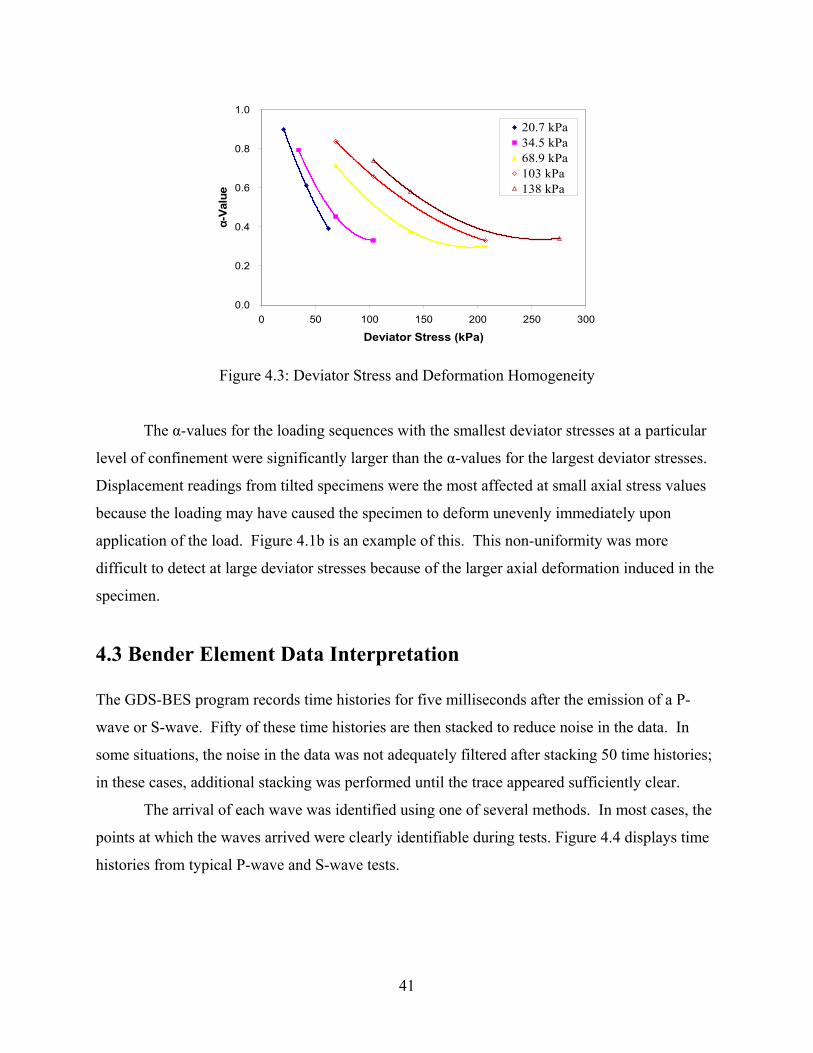
41
0.0
0.2
0.4
0.6
0.8
1.0
0 50 100 150 200 250 300
Deviator Stress (kPa)
α-Va
lue
20.7 kPa34.5 kPa68.9 kPa103 kPa138 kPa
Figure 4.3: Deviator Stress and Deformation Homogeneity
The α-values for the loading sequences with the smallest deviator stresses at a particular
level of confinement were significantly larger than the α-values for the largest deviator stresses.
Displacement readings from tilted specimens were the most affected at small axial stress values
because the loading may have caused the specimen to deform unevenly immediately upon
application of the load. Figure 4.1b is an example of this. This non-uniformity was more
difficult to detect at large deviator stresses because of the larger axial deformation induced in the
specimen.
4.3 Bender Element Data Interpretation
The GDS-BES program records time histories for five milliseconds after the emission of a P-
wave or S-wave. Fifty of these time histories are then stacked to reduce noise in the data. In
some situations, the noise in the data was not adequately filtered after stacking 50 time histories;
in these cases, additional stacking was performed until the trace appeared sufficiently clear.
The arrival of each wave was identified using one of several methods. In most cases, the
points at which the waves arrived were clearly identifiable during tests. Figure 4.4 displays time
histories from typical P-wave and S-wave tests.
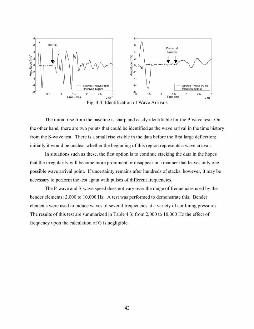
42
Fig. 4.4: Identification of Wave Arrivals
The initial rise from the baseline is sharp and easily identifiable for the P-wave test. On
the other hand, there are two points that could be identified as the wave arrival in the time history
from the S-wave test. There is a small rise visible in the data before the first large deflection;
initially it would be unclear whether the beginning of this region represents a wave arrival.
In situations such as these, the first option is to continue stacking the data in the hopes
that the irregularity will become more prominent or disappear in a manner that leaves only one
possible wave arrival point. If uncertainty remains after hundreds of stacks, however, it may be
necessary to perform the test again with pulses of different frequencies.
The P-wave and S-wave speed does not vary over the range of frequencies used by the
bender elements: 2,000 to 10,000 Hz. A test was performed to demonstrate this. Bender
elements were used to induce waves of several frequencies at a variety of confining pressures.
The results of this test are summarized in Table 4.3; from 2,000 to 10,000 Hz the effect of
frequency upon the calculation of G is negligible.
0 0.5 1 1.5 2 2.5 3x 10
-3
-8
-6
-4
-2
0
2
4
6
8
Time (ms)
Am
plitu
de [m
V]
Source P-wave PulseReceived Signal
Arrival
0 0.5 1 1.5 2 2.5 3x 10
-3
-8
-6
-4
-2
0
2
4
6
8
Time (ms)
Am
plitu
de [m
V]
Source P-wave PulseReceived Signal
Potential Arrivals
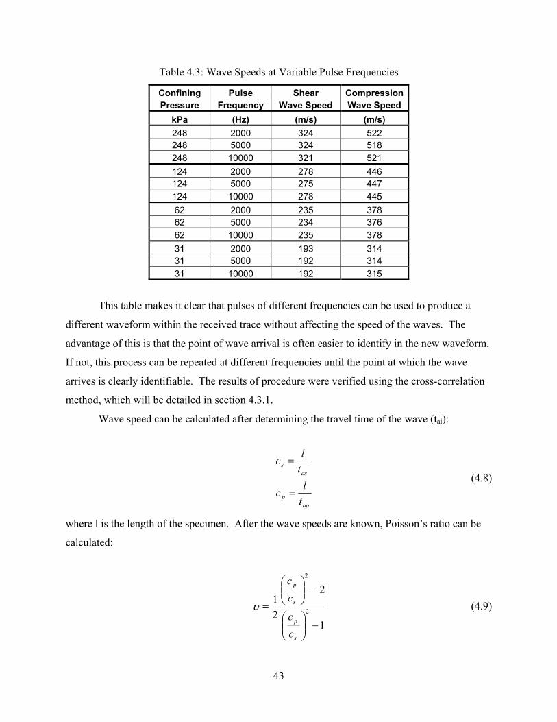
43
Table 4.3: Wave Speeds at Variable Pulse Frequencies
Confining Pulse Shear Compression Pressure Frequency Wave Speed Wave Speed
kPa (Hz) (m/s) (m/s) 248 2000 324 522 248 5000 324 518 248 10000 321 521 124 2000 278 446 124 5000 275 447 124 10000 278 445 62 2000 235 378 62 5000 234 376 62 10000 235 378 31 2000 193 314 31 5000 192 314 31 10000 192 315
This table makes it clear that pulses of different frequencies can be used to produce a
different waveform within the received trace without affecting the speed of the waves. The
advantage of this is that the point of wave arrival is often easier to identify in the new waveform.
If not, this process can be repeated at different frequencies until the point at which the wave
arrives is clearly identifiable. The results of procedure were verified using the cross-correlation
method, which will be detailed in section 4.3.1.
Wave speed can be calculated after determining the travel time of the wave (tai):
app
ass
tlc
tlc
=
=
(4.8)
where l is the length of the specimen. After the wave speeds are known, Poisson’s ratio can be
calculated:
1
2
21
2
2
−
−
=
s
p
s
p
cc
cc
υ (4.9)
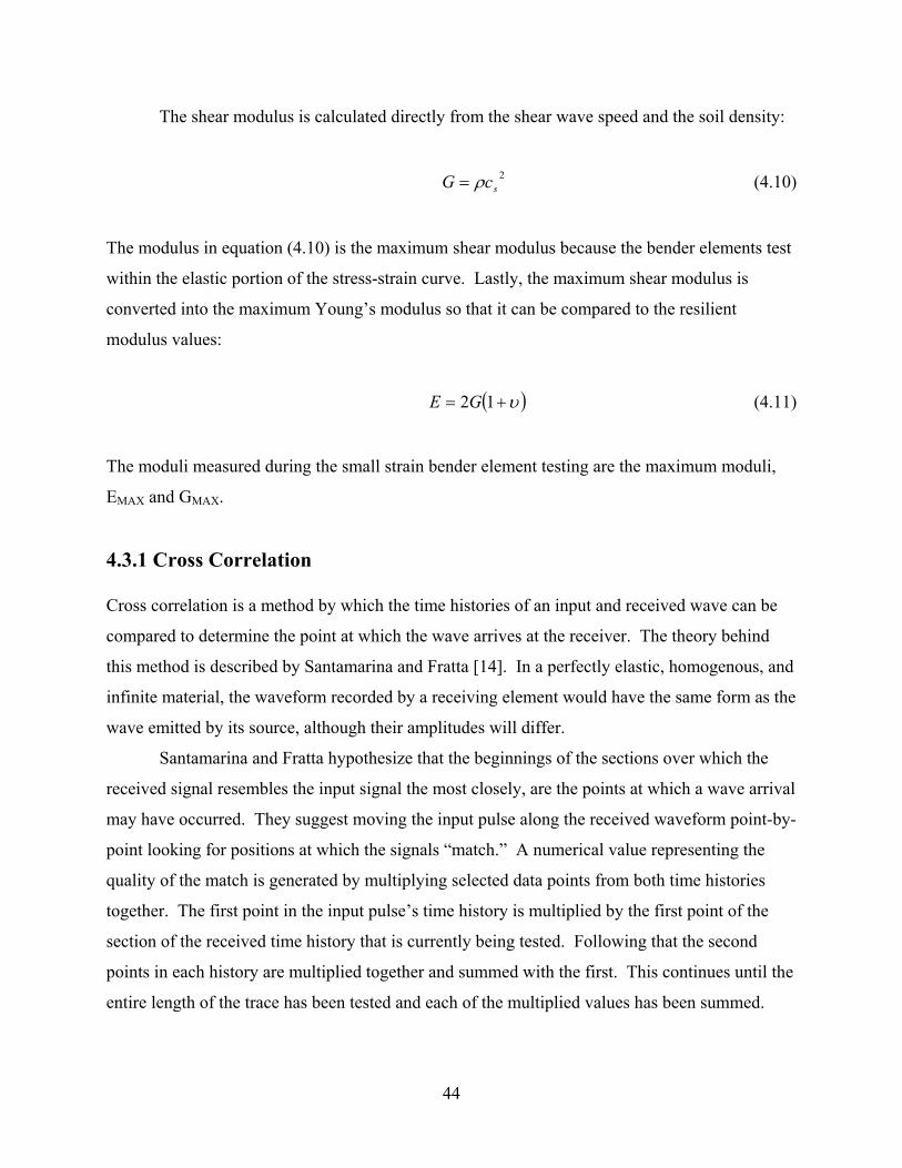
44
The shear modulus is calculated directly from the shear wave speed and the soil density:
2scG ρ= (4.10)
The modulus in equation (4.10) is the maximum shear modulus because the bender elements test
within the elastic portion of the stress-strain curve. Lastly, the maximum shear modulus is
converted into the maximum Young’s modulus so that it can be compared to the resilient
modulus values:
( )υ+= 12GE (4.11)
The moduli measured during the small strain bender element testing are the maximum moduli,
EMAX and GMAX.
4.3.1 Cross Correlation
Cross correlation is a method by which the time histories of an input and received wave can be
compared to determine the point at which the wave arrives at the receiver. The theory behind
this method is described by Santamarina and Fratta [14]. In a perfectly elastic, homogenous, and
infinite material, the waveform recorded by a receiving element would have the same form as the
wave emitted by its source, although their amplitudes will differ.
Santamarina and Fratta hypothesize that the beginnings of the sections over which the
received signal resembles the input signal the most closely, are the points at which a wave arrival
may have occurred. They suggest moving the input pulse along the received waveform point-by-
point looking for positions at which the signals “match.” A numerical value representing the
quality of the match is generated by multiplying selected data points from both time histories
together. The first point in the input pulse’s time history is multiplied by the first point of the
section of the received time history that is currently being tested. Following that the second
points in each history are multiplied together and summed with the first. This continues until the
entire length of the trace has been tested and each of the multiplied values has been summed.
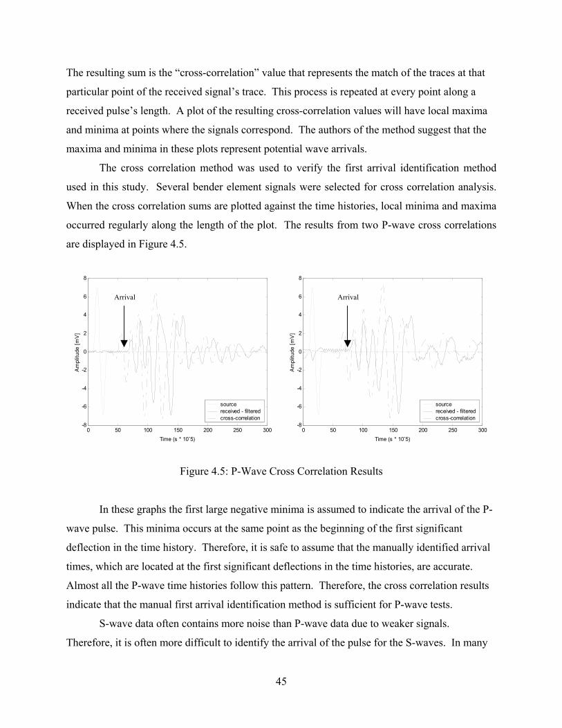
45
The resulting sum is the “cross-correlation” value that represents the match of the traces at that
particular point of the received signal’s trace. This process is repeated at every point along a
received pulse’s length. A plot of the resulting cross-correlation values will have local maxima
and minima at points where the signals correspond. The authors of the method suggest that the
maxima and minima in these plots represent potential wave arrivals.
The cross correlation method was used to verify the first arrival identification method
used in this study. Several bender element signals were selected for cross correlation analysis.
When the cross correlation sums are plotted against the time histories, local minima and maxima
occurred regularly along the length of the plot. The results from two P-wave cross correlations
are displayed in Figure 4.5.
Figure 4.5: P-Wave Cross Correlation Results
In these graphs the first large negative minima is assumed to indicate the arrival of the P-
wave pulse. This minima occurs at the same point as the beginning of the first significant
deflection in the time history. Therefore, it is safe to assume that the manually identified arrival
times, which are located at the first significant deflections in the time histories, are accurate.
Almost all the P-wave time histories follow this pattern. Therefore, the cross correlation results
indicate that the manual first arrival identification method is sufficient for P-wave tests.
S-wave data often contains more noise than P-wave data due to weaker signals.
Therefore, it is often more difficult to identify the arrival of the pulse for the S-waves. In many
0 50 100 150 200 250 300-8
-6
-4
-2
0
2
4
6
8
Time (s * 10-5)
Am
plitu
de [m
V]
source received - filteredcross-correlation
0 50 100 150 200 250 300-8
-6
-4
-2
0
2
4
6
8
Time (s * 10-5)
Am
plitu
de [m
V]
source received - filteredcross-correlation
Arrival Arrival

46
cases there is a shallow rise or depression before the first significant deflection in the time
history; it is important to know whether these deviations are physically significant. Figure 4.6
displays two cross-correlation results from S-wave time histories. The cross correlation in the
first plot conforms with expectations; the first significant cross correlation maxima appears over
the center of the small depression where the first significant deflection in the trace begins. The
cross correlation in the second plot, however, does not reach a minima or maxima over any
logical point; the first significant positive maxima in the cross correlation data occurs over a
point well after the first significant deflection in the S-wave time history. In this case the results
are inconclusive. In situations such as this experience must be used to identify the wave arrival.
Figure 4.6: S-Wave Cross Correlation Results
There are several potential explanations for why cross correlations may provide poor
results: poor homogeneity of the sample, electrical noise, and excessive wave reflections.
Fortunately, plots such as the first in Figure 4.6 are the most prevalent; the cross-correlation
method usually produces a peak over a possible arrival. Therefore, the results indicate that
manually identifying the first significant deflection of the time history is an accurate way to
determine wave arrival points.
0 50 100 150 200 250 300-8
-6
-4
-2
0
2
4
6
8
Time (s * 10-5)
Am
plitu
de [m
V]
source received - filteredcross-correlation
0 50 100 150 200 250 300-8
-6
-4
-2
0
2
4
6
8
Time (s * 10-5)
Am
plitu
de [m
V]
source received - filteredcross-correlation
Arrival Arrival
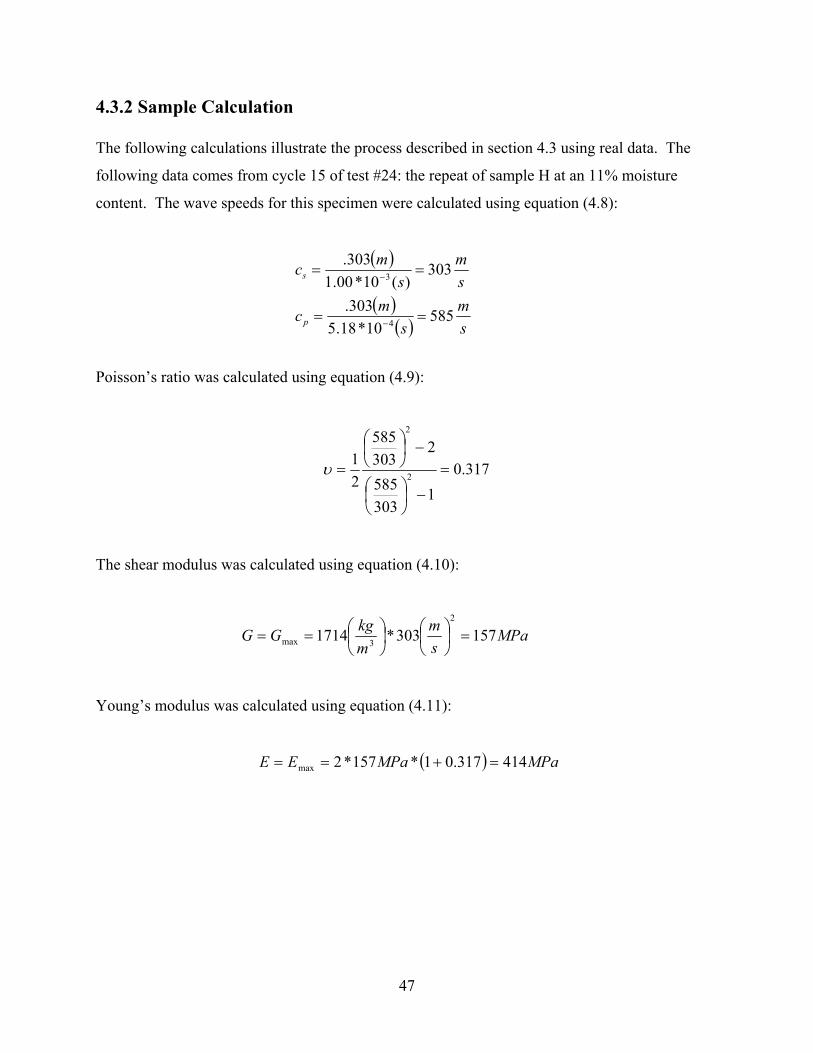
47
4.3.2 Sample Calculation
The following calculations illustrate the process described in section 4.3 using real data. The
following data comes from cycle 15 of test #24: the repeat of sample H at an 11% moisture
content. The wave speeds for this specimen were calculated using equation (4.8):
Poisson’s ratio was calculated using equation (4.9):
317.01
303585
2303585
21
2
2
=
−
−
=υ
The shear modulus was calculated using equation (4.10):
MPasm
mkgGG 157303*1714
2
3max =
==
Young’s modulus was calculated using equation (4.11):
( ) MPaMPaEE 414317.01*157*2max =+==
( )
( )( ) s
ms
mc
sm
smc
p
s
58510*18.5
303.
303)(10*00.1
303.
4
3
==
==
−
−
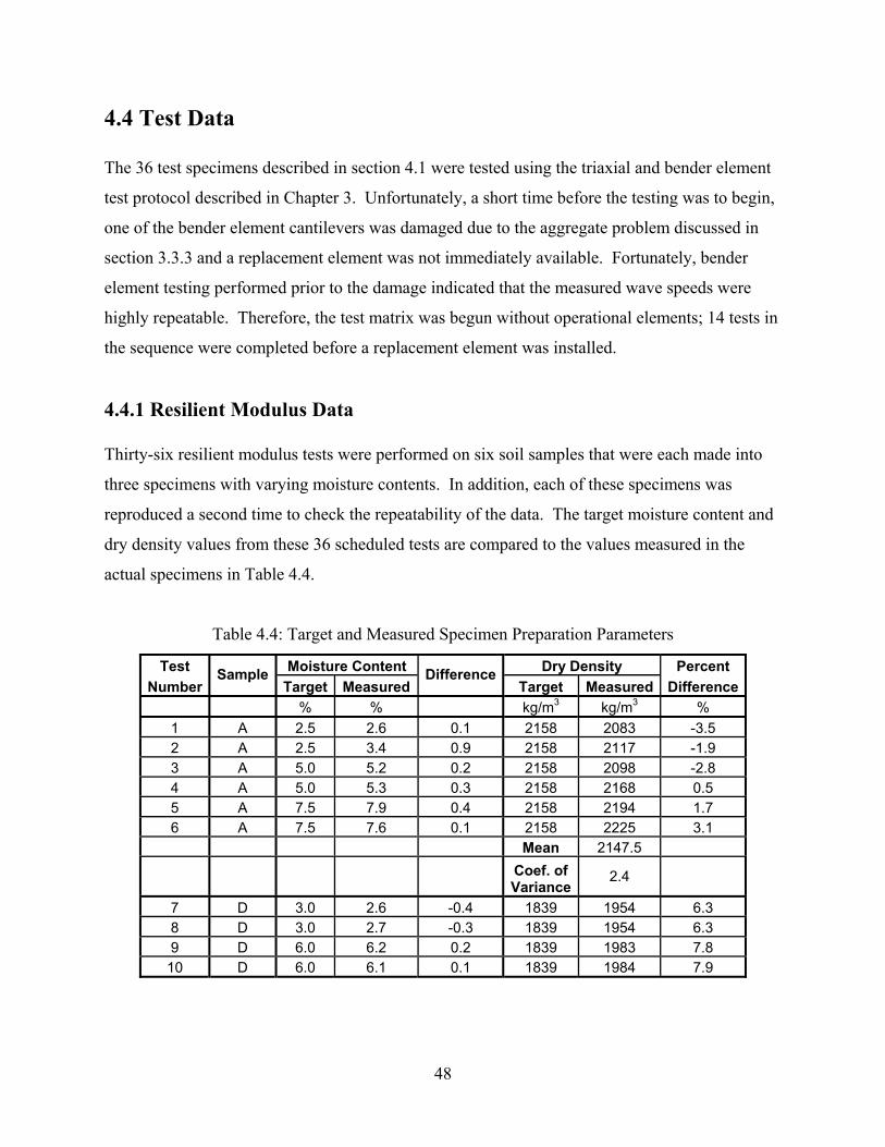
48
4.4 Test Data
The 36 test specimens described in section 4.1 were tested using the triaxial and bender element
test protocol described in Chapter 3. Unfortunately, a short time before the testing was to begin,
one of the bender element cantilevers was damaged due to the aggregate problem discussed in
section 3.3.3 and a replacement element was not immediately available. Fortunately, bender
element testing performed prior to the damage indicated that the measured wave speeds were
highly repeatable. Therefore, the test matrix was begun without operational elements; 14 tests in
the sequence were completed before a replacement element was installed.
4.4.1 Resilient Modulus Data
Thirty-six resilient modulus tests were performed on six soil samples that were each made into
three specimens with varying moisture contents. In addition, each of these specimens was
reproduced a second time to check the repeatability of the data. The target moisture content and
dry density values from these 36 scheduled tests are compared to the values measured in the
actual specimens in Table 4.4.
Table 4.4: Target and Measured Specimen Preparation Parameters
Test Moisture Content Dry Density Percent Number
Sample Target Measured
DifferenceTarget Measured Difference
% % kg/m3 kg/m3 % 1 A 2.5 2.6 0.1 2158 2083 -3.5 2 A 2.5 3.4 0.9 2158 2117 -1.9 3 A 5.0 5.2 0.2 2158 2098 -2.8 4 A 5.0 5.3 0.3 2158 2168 0.5 5 A 7.5 7.9 0.4 2158 2194 1.7 6 A 7.5 7.6 0.1 2158 2225 3.1 Mean 2147.5
Coef. ofVariance
2.4
7 D 3.0 2.6 -0.4 1839 1954 6.3 8 D 3.0 2.7 -0.3 1839 1954 6.3 9 D 6.0 6.2 0.2 1839 1983 7.8 10 D 6.0 6.1 0.1 1839 1984 7.9

49
Table 4.4 Continued: Target and Measured Specimen Preparation Parameters
Test Moisture Content Dry Density Percent Number
Sample Target Measured
DifferenceTarget Measured Difference
% % kg/m3 kg/m3 % 11 D 9.0 9.0 0.0 1839 1966 6.9 12 D 9.0 10.1 1.1 1839 1984 7.9
Mean 1975.0
Coef. ofVariance 0.5
13 F 3.5 3.2 -0.3 1900 1820 -4.2 14 F 3.5 3.4 -0.1 1900 1828 -3.8 15 F 6.0 5.7 -0.3 1900 1840 -3.2 16 F 6.0 6.3 0.3 1900 1857 -2.3 17 F 8.5 9.0 0.5 1900 1884 -0.8 18 F 8.5 7.3 -1.2 1900 1853 -2.5
Mean 1847.0
Coef. ofVariance 1.1
19 H 3.0 3.1 0.1 1725 1703 -1.3 20 H 3.0 3.5 0.5 1725 1732 0.4 21 H 7.0 7.4 0.4 1725 1760 2.0 22 H 7.0 7.1 0.1 1725 1760 2.0 23 H 11.0 11.0 0.0 1725 1786 3.5 24 H 11.0 10.6 -0.4 1725 1788 3.7
Mean 1754.8
Coef. ofVariance 1.7
25 J 3.5 3.3 -0.2 1791 1865 4.1 26 J 3.5 3.5 0.0 1791 1849 3.2 27 J 6.0 6.2 0.2 1791 1837 2.6 28 J 6.0 5.9 -0.1 1791 1858 3.7 29 J 8.5 7.9 -0.6 1791 1852 3.4 30 J 8.5 8.6 0.1 1791 1854 3.5
Mean 1852.5
Coef. ofVariance 0.5
31 N 3.0 3.2 0.2 2014 1929 -4.2 32 N 3.0 3.1 0.1 2014 1941 -3.6 33 N 5.5 5.5 0.0 2014 1980 -1.7 34 N 5.5 5.5 0.0 2014 2040 1.3 35 N 8.0 8.2 0.2 2014 2030 0.8 36 N 8.0 7.9 -0.1 2014 2064 2.5
Mean 2028.5
Coef. ofVariance 1.5

50
Several things about these data are noteworthy. To begin with, the target dry density
values proved to be difficult to achieve for many of the specimens. Samples such as D, H, and J
often became compacted to a value larger than the maximum dry density indicated by Mn/DOT’s
compaction curves almost immediately after the rotary hammer was placed in operation. On the
other end of the spectrum, sample F and some sample A and N specimens proved to be difficult
to compact to the intended density regardless of the compactive effort used. As a result, the
specimen unit densities vary to a degree. However, the majority are within 5% of the target
value.
The measured moisture content of the specimens was usually within ±0.5% of the target
moisture content as required by LTPP P46. Only three of the 36 tests fell outside of this range,
and none of the three was more than 1.0% away from its target.
Figure 4.7 contains plots of the resilient modulus data generated from the 36 specimens
in Table 4.4. A different plot was created for each sample, and the three trendlines on each of the
plots were calculated using the data from the specimens prepared at each of the soil’s three
moisture contents. Similar plots that include the data from the bender elements were generated
for each moisture content. These plots are included in Appendix D.1.
The resilient modulus values recorded during this series of testing tended to decrease as
the moisture content of the specimens increased. Sample N (Figure 4.7f) was the only
significant exception; the trendline calculated for the 8.0% moisture content plotted directly over
the trendline for the 3.0% moisture content. However, in the case of N all three of the trendlines
were located within a small range; further testing of sample N may prove this result to be a
sample size error. The increase in MR with decrease in moisture content may be related to the
compactive effort used to reach the maximum dry density. In addition, the specimens created at
smaller moisture contents were found to have significantly larger values of cohesion. Cohesion
and the shear strength data are discussed in section 4.4.4.
Figure 4.7 also makes it clear that some of the data was difficult to repeat. The
specimens created by compacting sample J at a 3.5% moisture content (Figure 4.7e), for
example, produced MR values that differ from each other by almost 50%. Fortunately, the
majority of the specimens generated data that were within 20% of their repeat.
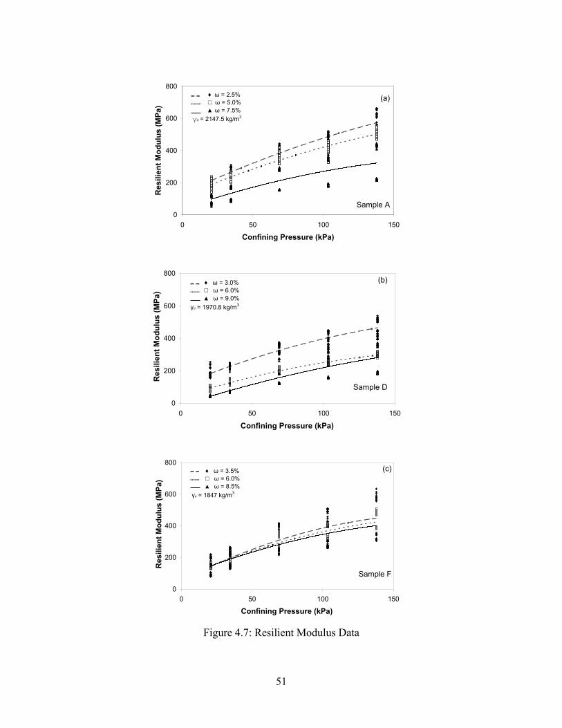
51
0
200
400
600
800
0 50 100 150
Confining Pressure (kPa)
Res
ilien
t Mod
ulus
(MPa
)
♦ ω = 2.5% □ ω = 5.0% ▲ ω = 7.5% γd = 2147.5 kg/m3
(a)
Sample A
0
200
400
600
800
0 50 100 150
Confining Pressure (kPa)
Res
ilien
t Mod
ulus
(MPa
)
♦ ω = 3.0% □ ω = 6.0% ▲ ω = 9.0% γd = 1970.8 kg/m3
(b)
Sample D
0
200
400
600
800
0 50 100 150
Confining Pressure (kPa)
Res
ilien
t Mod
ulus
(MPa
)
(c)
Sample F
♦ ω = 3.5% □ ω = 6.0% ▲ ω = 8.5% γd = 1847 kg/m3
Figure 4.7: Resilient Modulus Data

52
0
200
400
600
800
0 50 100 150
Confining Pressure (kPa)
Res
ilien
t Mod
ulus
(MPa
)
♦ ω = 3.0% □ ω = 7.0% ▲ ω = 11.0% γd = 1754.8 kg/m3
(d)
Sample H
0
200
400
600
800
0 50 100 150
Confining Pressure (kPa)
Res
ilien
t Mod
ulus
(MPa
)
♦ ω = 3.5% □ ω = 6.0% ▲ ω = 8.5% γd = 1852.5 kg/m3
(e)
Sample J
0
200
400
600
800
0 50 100 150
Confining Pressure (kPa)
Res
ilien
t Mod
ulus
(MPa
)
♦ ω = 3.0% □ ω = 5.5% ▲ ω = 8.0% γd = 2034.7 kg/m3
(f)
Sample N
Figure 4.7 Continued: Resilient Modulus Data
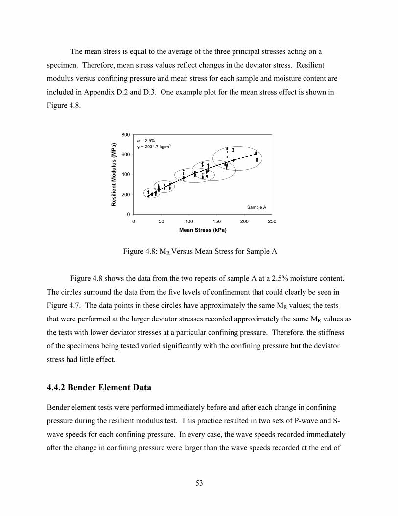
53
The mean stress is equal to the average of the three principal stresses acting on a
specimen. Therefore, mean stress values reflect changes in the deviator stress. Resilient
modulus versus confining pressure and mean stress for each sample and moisture content are
included in Appendix D.2 and D.3. One example plot for the mean stress effect is shown in
Figure 4.8.
0
200
400
600
800
0 50 100 150 200 250
Mean Stress (kPa)
Res
ilien
t Mod
ulus
(MPa
) ω = 2.5%γd = 2034.7 kg/m3
Sample A
Figure 4.8: MR Versus Mean Stress for Sample A
Figure 4.8 shows the data from the two repeats of sample A at a 2.5% moisture content.
The circles surround the data from the five levels of confinement that could clearly be seen in
Figure 4.7. The data points in these circles have approximately the same MR values; the tests
that were performed at the larger deviator stresses recorded approximately the same MR values as
the tests with lower deviator stresses at a particular confining pressure. Therefore, the stiffness
of the specimens being tested varied significantly with the confining pressure but the deviator
stress had little effect.
4.4.2 Bender Element Data
Bender element tests were performed immediately before and after each change in confining
pressure during the resilient modulus test. This practice resulted in two sets of P-wave and S-
wave speeds for each confining pressure. In every case, the wave speeds recorded immediately
after the change in confining pressure were larger than the wave speeds recorded at the end of

54
the confining pressure’s loading sequences, although each of the changes was smaller than 2% of
the first wave speed measured. This decline in wave speed was most likely the result of
permanent deformations, from change in length (<1%) and change in volume, taking place
within the specimen during the loading sequences. For example, these deformations reduced the
volume of the specimen and, because the wave speeds are inversely proportional to material
density, the waves slowed in the higher density soil after loading sequences. Fortunately, the
difference between the two wave speeds was small; most values differed by no more than 2%.
The reported EMAX values are the averaged results from both wave speed measurements. These
values are compared with the MR values produced during the three loading sequences that took
place between the changes in confining pressure.
Direct comparisons between EMAX and MR for each soil at each moisture content are
included in appendix D.1. Figure 4.9 contains an example of these plots. The majority of the
plots appear similar to this curve; the bender element data follows a trend similar to the MR data
at larger values.
0
200
400
600
800
1000
0 50 100 150
Confining Pressure (kPa)
Youn
g's
Mod
ulus
(MPa
) Resilient ModulusBender Elements
Sample Aω = 5.0%
Figure 4.9: MR and EMAX Curves
Figure 4.10 contains the bender element data from each of the soils. These data are in
good agreement with the MR data; in most cases, the specimens with smaller moisture contents
have larger EMAX values. However, the specimens from sample F (Figure 4.10c) and sample J
(Figure 4.10e) were exceptions. Sample F had unusually

55
0
200
400
600
800
1000
0 50 100 150
Confining Pressure (kPa)
Youn
g's
Mod
ulus
(MPa
)
ω = 2.5%
ω = 5.0%
ω = 7.5%
(a)
Sample A
γd = 2147.5 kg/m3
0
200
400
600
800
1000
0 50 100 150
Confining Pressure (kPa)
Youn
g's
Mod
ulus
(MPa
)
ω = 3.0%
ω = 6.0%
ω = 9.0%
(b)
Sample D
γd = 1970.8 kg/m3
0
200
400
600
800
1000
0 50 100 150
Confining Pressure (kPa)
Youn
g's
Mod
ulus
(MPa
)
ω = 3.5%
ω = 6.0%
ω = 8.5%
(c)
Sample F
γd = 1847 kg/m3
Figure 4.10: Bender Element Data
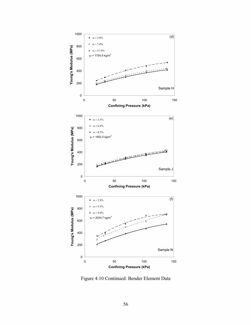
56
0
200
400
600
800
1000
0 50 100 150
Confining Pressure (kPa)
Youn
g's
Mod
ulus
(MPa
)
ω = 3.0%
ω = 7.0%
ω = 11.0%
(d)
Sample H
γd = 1754.8 kg/m3
0
200
400
600
800
1000
0 50 100 150
Confining Pressure (kPa)
Youn
g's
Mod
ulus
(MPa
)
ω = 3.5%
ω = 6.0%
ω = 8.5%
(e)
Sample J
γd = 1852.5 kg/m3
0
200
400
600
800
1000
0 50 100 150
Confining Pressure (kPa)
Youn
g's
Mod
ulus
(MPa
)
ω = 3.0%
ω = 5.5%
ω = 8.0%
(f)
Sample N
γd = 2034.7 kg/m3
Figure 4:10 Continued: Bender Element Data

57
large stiffnesses at a moisture content of 6% and small confinement; sample J had stiffnesses that
were similar in magnitude at every moisture content. Sample J more likely acted differently
from the other samples because of its poor gradation and small fine content. The discrepancy
recorded in sample F was most likely a sample size error.
EMAX and MR data from each level of confinement can be seen in Table 4.5.
Table 4.5: Resilient Modulus and EMAX
MR E Confinement (kPa) Confinement (kPa)
Test Number
20.7 34.5 68.9 103 138 20.7 34.5 68.9 103 138
(Sample) (MPa) (MPa) 1 (A) 217 285 421 499 632 - - - - - 2 (A) 193 256 380 430 530 435 521 728 833 958 3 (A) 163 222 336 384 504 - - - - - 4 (A) 203 255 376 432 516 299 354 524 631 688 5 (A) 72 92 156 184 219 - - - - - 6 (A) 119 173 284 350 431 147 225 353 452 509 7 (D) 201 240 359 424 516 - - - - - 8 (D) 162 210 312 360 421 265 315 433 533 612 9 (D) 74 116 194 243 298 - - - - - 10 (D) 104 142 217 250 300 189 249 361 443 508 11 (D) 48 73 124 159 189 - - - - - 12 (D) 45 72 193 295 372 181 52 158 234 271 13 (F) 189 245 403 477 582 - - - - - 14 (F) 92 143 240 281 323 129 217 328 409 459 15 (F) 134 171 262 306 373 169 204 297 362 424 16 (F) 155 221 346 403 485 228 280 384 456 511 17 (F) 133 173 277 328 386 157 282 411 480 548 18 (F) 158 203 305 355 424 251 318 438 514 575 19 (H) 137 183 266 318 372 - - - - - 20 (H) 135 170 260 299 362 244 296 411 480 538 21 (H) 130 174 257 306 358 174 217 302 356 399 22 (H) 167 230 338 407 429 226 267 351 438 481 23 (H) 98 142 222 263 309 145 183 273 330 372 24 (H) 153 194 277 327 373 214 266 326 418 464

58
Table 4.5 Continued: Resilient Modulus and EMAX
MR E Confinement (kPa) Confinement (kPa)
Test Number
20.7 34.5 68.9 103 138 20.7 34.5 68.9 103 138
(Sample) (MPa) (MPa) 25 (J) 260 341 481 591 697 - - - - - 26 (J) 137 194 284 329 394 165 217 308 364 418 27 (J) 150 198 284 332 391 - - - - - 28 (J) 138 194 282 333 392 188 230 316 376 434 29 (J) 184 229 320 371 440 - - - - - 30 (J) 149 200 281 320 377 162 209 292 347 406 31 (N) 197 236 345 419 475 - - - - - 32 (N) 230 285 409 504 574 350 400 547 689 699 33 (N) 166 222 342 428 493 - - - - - 34 (N) 177 242 373 437 533 285 383 499 584 715 35 (N) 88 135 225 273 336 - - - - - 36 (N) 140 186 276 332 400 208 273 390 467 548
The data missing from this table are from the tests in which the bender elements were damaged.
Fortunately, at least one set of bender element data was created for each target moisture content
of each sample. Table 4.6 shows the elastic parameters estimated from bender element testing.
Table 4.6: Elastic Parameters Estimated from Bender Element Testing
E G ν
Confinement (kPa) Confinement (kPa) Confinement (kPa) Test Num ber
20.7 34.5 68.9 103 138 20.7 34.5 68.9 103 138 20.7 34.5 68.9 103 138
(MPa) (MPa)
2 (A) 435 521 728 833 958 158 188 265 305 352 0.38 0.38 0.37 0.37 0.36
4 (A) 299 354 524 631 688 109 129 192 232 251 0.37 0.37 0.37 0.36 0.37
6 (A) 147 225 353 452 509 54 83 131 167 189 0.36 0.36 0.35 0.35 0.35
8 (D) 265 315 433 533 612 96 115 159 198 227 0.38 0.37 0.36 0.35 0.35
10 (D) 189 249 361 443 508 76 101 153 186 215 0.24 0.23 0.18 0.19 0.18

59
Table 4.6 Continued: Elastic Parameters Estimated from Bender Element Testing
E G ν
Confinement (kPa) Confinement (kPa) Confinement (kPa) Test Num ber
20.7 34.5 68.9 103 138 20.7 34.5 68.9 103 138 20.7 34.5 68.9 103 138
(MPa) (MPa)
14 (F) 129 217 328 409 459 46 80 121 153 171 0.4 0.36 0.35 0.34 0.34
15 (F) 169 204 297 362 424 62 76 111 136 160 0.35 0.35 0.34 0.33 0.33
16 (F) 228 280 384 456 511 85 104 143 171 193 0.35 0.35 0.34 0.33 0.32
17 (F) 157 282 411 480 548 63 116 170 198 224 0.26 0.22 0.21 0.22 0.22
18 (F) 251 318 438 514 575 91 117 163 190 214 0.38 0.36 0.34 0.35 0.34
20 (H) 244 296 411 480 538 92 111 157 182 206 0.33 0.33 0.31 0.32 0.31
21 (H) 174 217 302 356 399 64 81 113 133 150 0.35 0.34 0.34 0.34 0.33
22 (H) 226 267 351 438 481 84 100 131 166 183 0.35 0.34 0.34 0.32 0.32
23 (H) 145 183 273 330 372 54 69 103 126 142 0.34 0.32 0.32 0.31 0.31
24 (H) 214 266 326 418 464 79 99 121 158 176 0.36 0.35 0.35 0.32 0.32
26 (J) 165 217 308 364 418 62 83 119 142 163 0.34 0.31 0.29 0.28 0.28
28 (J) 188 230 316 376 434 69 86 120 143 164 0.36 0.34 0.32 0.32 0.32
30 (J) 162 209 292 347 406 61 79 112 133 156 0.33 0.32 0.31 0.3 0.3
32 (N) 350 400 547 689 699 126 144 198 252 253 0.38 0.39 0.38 0.37 0.38
34 (N) 285 383 499 584 715 105 141 184 215 267 0.36 0.36 0.35 0.36 0.34
36 (N) 208 273 390 467 548 77 102 147 177 209 0.35 0.34 0.33 0.32 0.31
4.4.3 Percometer Data
Three Percometer tests were performed across the diameter of the surface of each specimen.
These tests measure the dielectric permittivity and conductivity values of the soil being tested,
which can be used to estimate the volumetric moisture content of the soil being tested. The raw
data from this testing is contained in Table 4.7.
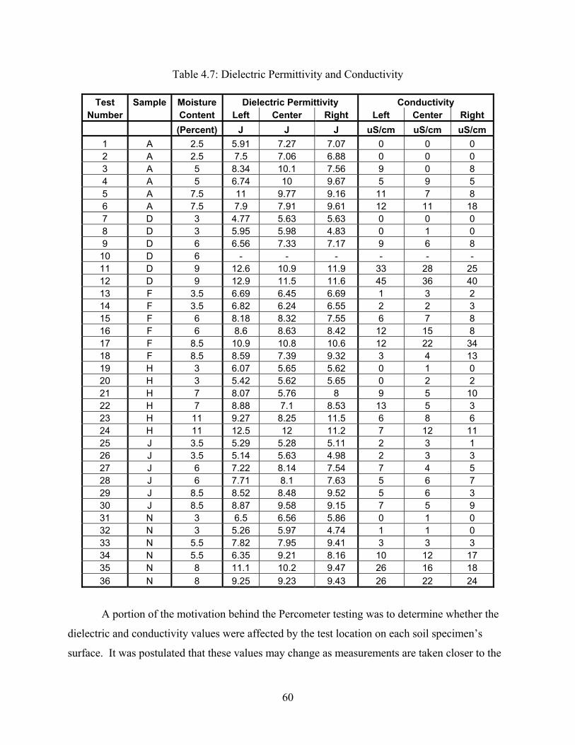
60
Table 4.7: Dielectric Permittivity and Conductivity
Test Sample Moisture Dielectric Permittivity Conductivity Number Content Left Center Right Left Center Right
(Percent) J J J uS/cm uS/cm uS/cm 1 A 2.5 5.91 7.27 7.07 0 0 0 2 A 2.5 7.5 7.06 6.88 0 0 0 3 A 5 8.34 10.1 7.56 9 0 8 4 A 5 6.74 10 9.67 5 9 5 5 A 7.5 11 9.77 9.16 11 7 8 6 A 7.5 7.9 7.91 9.61 12 11 18 7 D 3 4.77 5.63 5.63 0 0 0 8 D 3 5.95 5.98 4.83 0 1 0 9 D 6 6.56 7.33 7.17 9 6 8 10 D 6 - - - - - - 11 D 9 12.6 10.9 11.9 33 28 25 12 D 9 12.9 11.5 11.6 45 36 40 13 F 3.5 6.69 6.45 6.69 1 3 2 14 F 3.5 6.82 6.24 6.55 2 2 3 15 F 6 8.18 8.32 7.55 6 7 8 16 F 6 8.6 8.63 8.42 12 15 8 17 F 8.5 10.9 10.8 10.6 12 22 34 18 F 8.5 8.59 7.39 9.32 3 4 13 19 H 3 6.07 5.65 5.62 0 1 0 20 H 3 5.42 5.62 5.65 0 2 2 21 H 7 8.07 5.76 8 9 5 10 22 H 7 8.88 7.1 8.53 13 5 3 23 H 11 9.27 8.25 11.5 6 8 6 24 H 11 12.5 12 11.2 7 12 11 25 J 3.5 5.29 5.28 5.11 2 3 1 26 J 3.5 5.14 5.63 4.98 2 3 3 27 J 6 7.22 8.14 7.54 7 4 5 28 J 6 7.71 8.1 7.63 5 6 7 29 J 8.5 8.52 8.48 9.52 5 6 3 30 J 8.5 8.87 9.58 9.15 7 5 9 31 N 3 6.5 6.56 5.86 0 1 0 32 N 3 5.26 5.97 4.74 1 1 0 33 N 5.5 7.82 7.95 9.41 3 3 3 34 N 5.5 6.35 9.21 8.16 10 12 17 35 N 8 11.1 10.2 9.47 26 16 18 36 N 8 9.25 9.23 9.43 26 22 24
A portion of the motivation behind the Percometer testing was to determine whether the
dielectric and conductivity values were affected by the test location on each soil specimen’s
surface. It was postulated that these values may change as measurements are taken closer to the
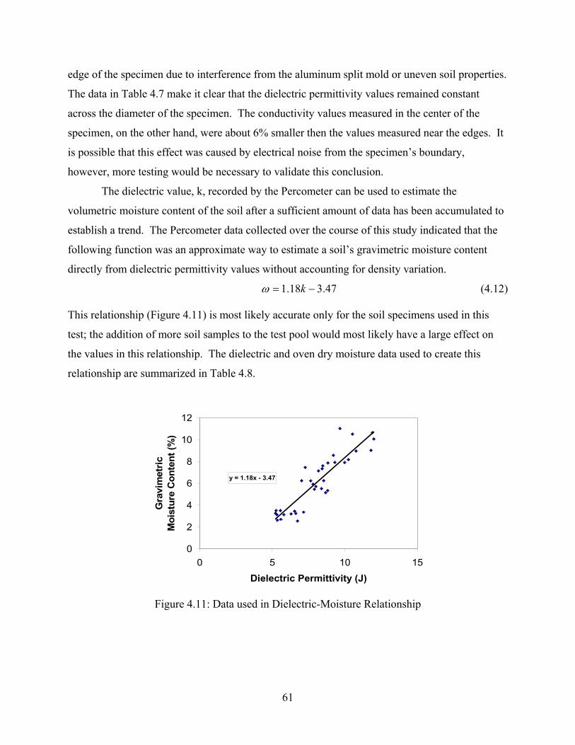
61
edge of the specimen due to interference from the aluminum split mold or uneven soil properties.
The data in Table 4.7 make it clear that the dielectric permittivity values remained constant
across the diameter of the specimen. The conductivity values measured in the center of the
specimen, on the other hand, were about 6% smaller then the values measured near the edges. It
is possible that this effect was caused by electrical noise from the specimen’s boundary,
however, more testing would be necessary to validate this conclusion.
The dielectric value, k, recorded by the Percometer can be used to estimate the
volumetric moisture content of the soil after a sufficient amount of data has been accumulated to
establish a trend. The Percometer data collected over the course of this study indicated that the
following function was an approximate way to estimate a soil’s gravimetric moisture content
directly from dielectric permittivity values without accounting for density variation.
47.318.1 −= kω (4.12)
This relationship (Figure 4.11) is most likely accurate only for the soil specimens used in this
test; the addition of more soil samples to the test pool would most likely have a large effect on
the values in this relationship. The dielectric and oven dry moisture data used to create this
relationship are summarized in Table 4.8.
y = 1.18x - 3.47
0
2
4
6
8
10
12
0 5 10 15Dielectric Permittivity (J)
Gra
vim
etric
Moi
stur
e C
onte
nt (%
)
Figure 4.11: Data used in Dielectric-Moisture Relationship

62
Table 4.8: Dielectric Moisture Content Estimates
Percometer Results Gravimetric Moisture Content
Test # Sample Dielectric Conductivity Target
Measuredfrom Oven
Predicted from
Dielectric Difference
J uS/cm % % % % 1 A 6.75 0.00 2.5 2.55 4.46 1.91 2 A 7.15 0.00 2.5 3.35 4.72 1.37 3 A 8.67 5.67 5 5.15 5.72 0.57 4 A 8.80 6.33 5 5.34 5.81 0.47 5 A 9.98 8.67 7.5 7.89 6.58 -1.31 6 A 8.47 13.67 7.5 7.61 5.59 -2.02 7 D 5.34 0.00 3 2.63 3.53 0.90 8 D 5.59 0.33 3 2.70 3.69 0.99 9 D 7.02 7.67 6 6.24 4.63 -1.61
10 D - - 6 6.10 - - 11 D 11.80 28.67 9 9.01 7.79 -1.22 12 D 12.00 40.33 9 10.06 7.92 -2.14 13 F 6.61 2.00 3.5 3.23 4.36 1.13 14 F 6.54 2.33 3.5 3.44 4.31 0.87 15 F 8.02 7.00 6 5.7 5.29 -0.41 16 F 8.55 11.67 6 6.25 5.64 -0.61 17 F 10.77 22.67 8.5 8.96 7.11 -1.85 18 F 8.43 6.67 8.5 7.33 5.57 -1.76 19 H 5.78 0.33 3 3.13 3.81 0.68 20 H 5.56 1.33 3 3.49 3.67 0.18 21 H 7.28 8.00 7 7.44 4.80 -2.64 22 H 8.17 7.00 7 7.13 5.39 -1.74 23 H 9.67 6.67 11 11.01 6.38 -4.63 24 H 11.90 10.00 11 10.64 7.85 -2.79 25 J 5.23 2.00 3.5 3.26 3.45 0.19 26 J 5.25 2.67 3.5 3.49 3.47 -0.03 27 J 7.63 5.33 6 6.22 5.04 -1.18 28 J 7.81 6.00 6 5.93 5.16 -0.77 29 J 8.84 4.67 8.5 7.88 5.83 -2.05 30 J 9.20 7.00 8.5 8.56 6.07 -2.49 31 N 6.31 0.33 3 3.20 4.16 0.96 32 N 5.32 0.67 3 3.12 3.51 0.39 33 N 8.39 3.00 5.5 5.50 5.54 0.04 34 N 7.91 13.00 5.5 5.45 5.22 -0.23 35 N 10.26 20.00 8 8.16 6.77 -1.39 36 N 9.30 24.00 8 7.90 6.14 -1.76
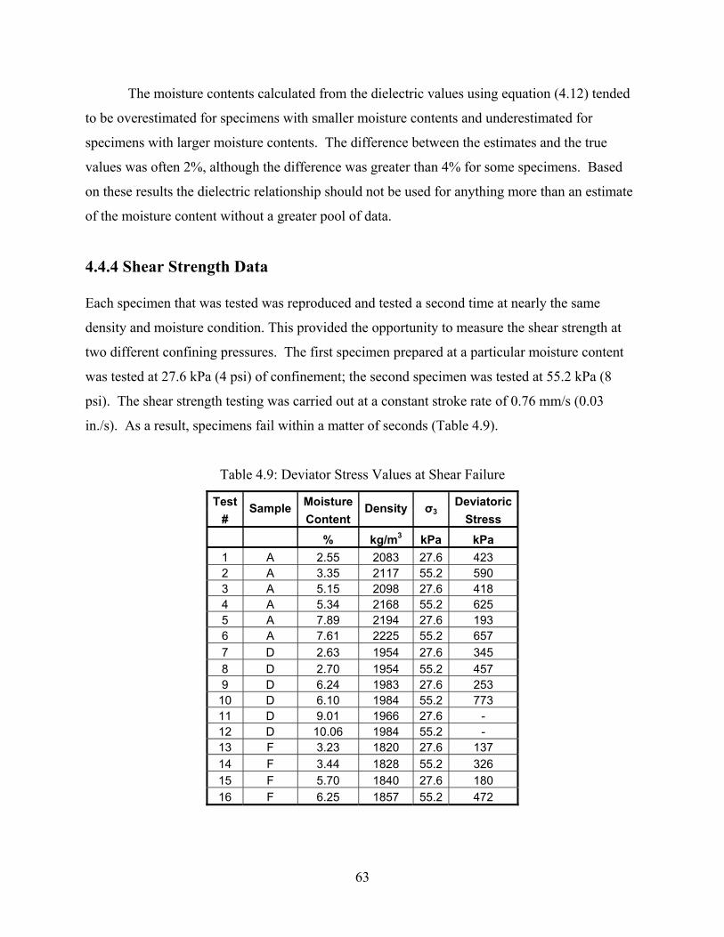
63
The moisture contents calculated from the dielectric values using equation (4.12) tended
to be overestimated for specimens with smaller moisture contents and underestimated for
specimens with larger moisture contents. The difference between the estimates and the true
values was often 2%, although the difference was greater than 4% for some specimens. Based
on these results the dielectric relationship should not be used for anything more than an estimate
of the moisture content without a greater pool of data.
4.4.4 Shear Strength Data
Each specimen that was tested was reproduced and tested a second time at nearly the same
density and moisture condition. This provided the opportunity to measure the shear strength at
two different confining pressures. The first specimen prepared at a particular moisture content
was tested at 27.6 kPa (4 psi) of confinement; the second specimen was tested at 55.2 kPa (8
psi). The shear strength testing was carried out at a constant stroke rate of 0.76 mm/s (0.03
in./s). As a result, specimens fail within a matter of seconds (Table 4.9).
Table 4.9: Deviator Stress Values at Shear Failure
Test Moisture Deviatoric #
SampleContent
Density σ3 Stress
% kg/m3 kPa kPa 1 A 2.55 2083 27.6 423 2 A 3.35 2117 55.2 590 3 A 5.15 2098 27.6 418 4 A 5.34 2168 55.2 625 5 A 7.89 2194 27.6 193 6 A 7.61 2225 55.2 657 7 D 2.63 1954 27.6 345 8 D 2.70 1954 55.2 457 9 D 6.24 1983 27.6 253
10 D 6.10 1984 55.2 773 11 D 9.01 1966 27.6 - 12 D 10.06 1984 55.2 - 13 F 3.23 1820 27.6 137 14 F 3.44 1828 55.2 326 15 F 5.70 1840 27.6 180 16 F 6.25 1857 55.2 472

64
Table 4.9 Continued: Deviator Stress Values at Shear Failure
Test Moisture Deviatoric #
SampleContent
Density σ3 Stress
% kg/m3 kPa kPa 17 F 8.96 1884 27.6 156 18 F 7.33 1853 55.2 462 19 H 3.13 1703 27.6 259 20 H 3.49 1732 55.2 411 21 H 7.44 1760 27.6 158 22 H 7.13 1760 55.2 414 23 H 11.01 1786 27.6 199 24 H 10.64 1788 55.2 353 25 J 3.26 1865 27.6 203 26 J 3.49 1849 55.2 298 27 J 6.22 1837 27.6 183 28 J 5.93 1858 55.2 299 29 J 7.88 1852 27.6 189 30 J 8.56 1854 55.2 305 31 N 3.20 1929 27.6 351 32 N 3.12 1941 55.2 457 33 N 5.50 1980 27.6 417 34 N 5.45 2040 55.2 575 35 N 8.16 2030 27.6 321 36 N 7.90 2064 55.2 545
The data from these tests can be used to calculate the friction angle and cohesion for each
soil; these quantities are useful in a number of applications. In particular, the data can be used to
calculate E/EMAX curves using the hyperbolic model; this process is explained in section 4.5.
The friction angle (φ) and cohesion (c) values can be calculated by plotting both shear strength
tests, which were performed at 27.6 and 55.2 kPa, on the same principal stress plot, σ1 versus σ3:
31 2 σσ pp KKc += (4.13)
φφ
sin1sin1
−+
=pK
The slope of the trendline formed by the two points, Kp, is needed to calculate the friction angle
of the specimen. Once the friction angle is known, the cohesion can be calculated from the y-
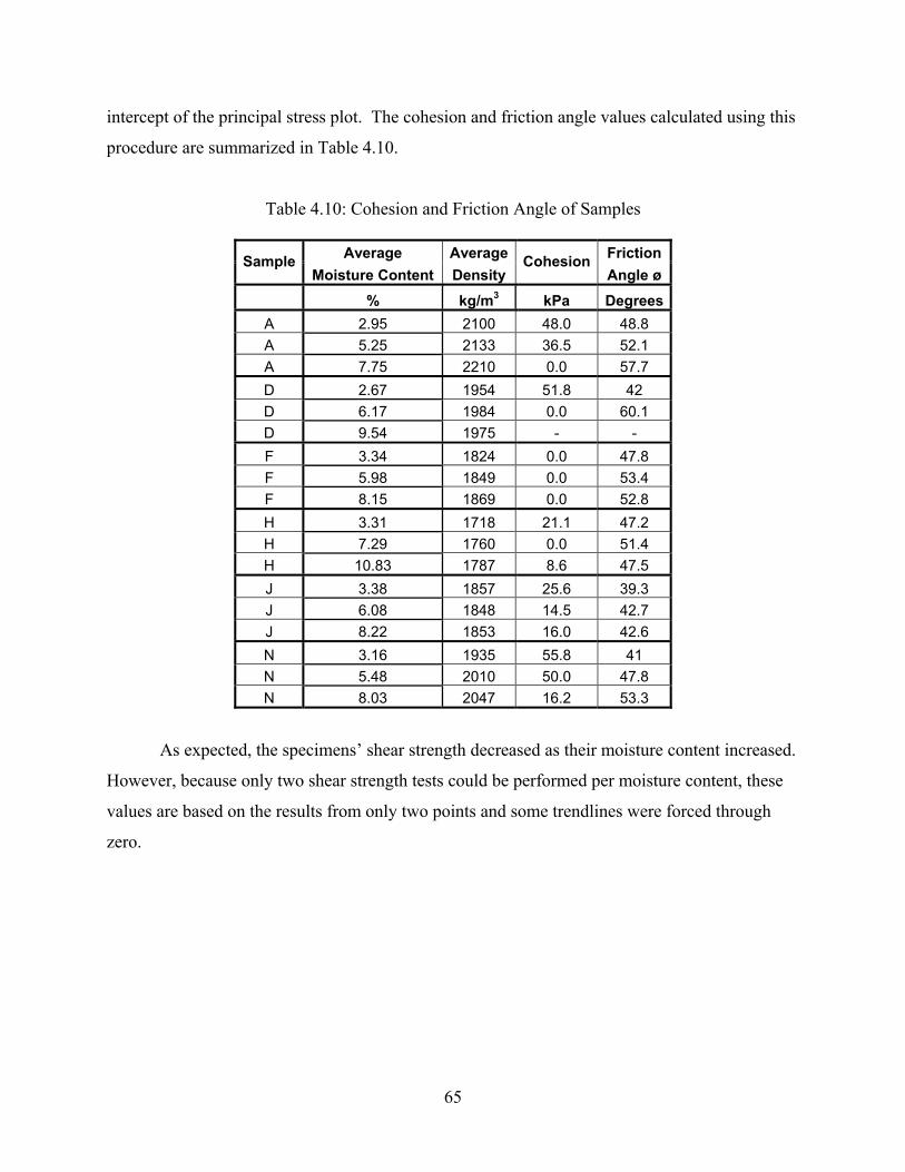
65
intercept of the principal stress plot. The cohesion and friction angle values calculated using this
procedure are summarized in Table 4.10.
Table 4.10: Cohesion and Friction Angle of Samples
Average Average Friction Sample Moisture Content Density
CohesionAngle ø
% kg/m3 kPa Degrees A 2.95 2100 48.0 48.8 A 5.25 2133 36.5 52.1 A 7.75 2210 0.0 57.7 D 2.67 1954 51.8 42 D 6.17 1984 0.0 60.1 D 9.54 1975 - - F 3.34 1824 0.0 47.8 F 5.98 1849 0.0 53.4 F 8.15 1869 0.0 52.8 H 3.31 1718 21.1 47.2 H 7.29 1760 0.0 51.4 H 10.83 1787 8.6 47.5 J 3.38 1857 25.6 39.3 J 6.08 1848 14.5 42.7 J 8.22 1853 16.0 42.6 N 3.16 1935 55.8 41 N 5.48 2010 50.0 47.8 N 8.03 2047 16.2 53.3
As expected, the specimens’ shear strength decreased as their moisture content increased.
However, because only two shear strength tests could be performed per moisture content, these
values are based on the results from only two points and some trendlines were forced through
zero.
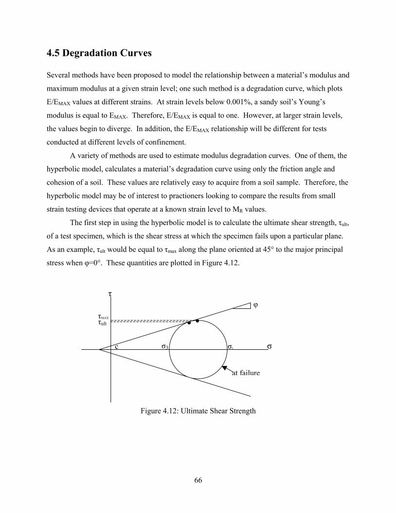
66
4.5 Degradation Curves
Several methods have been proposed to model the relationship between a material’s modulus and
maximum modulus at a given strain level; one such method is a degradation curve, which plots
E/EMAX values at different strains. At strain levels below 0.001%, a sandy soil’s Young’s
modulus is equal to EMAX. Therefore, E/EMAX is equal to one. However, at larger strain levels,
the values begin to diverge. In addition, the E/EMAX relationship will be different for tests
conducted at different levels of confinement.
A variety of methods are used to estimate modulus degradation curves. One of them, the
hyperbolic model, calculates a material’s degradation curve using only the friction angle and
cohesion of a soil. These values are relatively easy to acquire from a soil sample. Therefore, the
hyperbolic model may be of interest to practioners looking to compare the results from small
strain testing devices that operate at a known strain level to MR values.
The first step in using the hyperbolic model is to calculate the ultimate shear strength, τult,
of a test specimen, which is the shear stress at which the specimen fails upon a particular plane.
As an example, τult would be equal to τmax along the plane oriented at 45° to the major principal
stress when φ=0°. These quantities are plotted in Figure 4.12.
Figure 4.12: Ultimate Shear Strength
τMAX φ
τ
σ
τult
σ1 σ3
at failure
c
• •
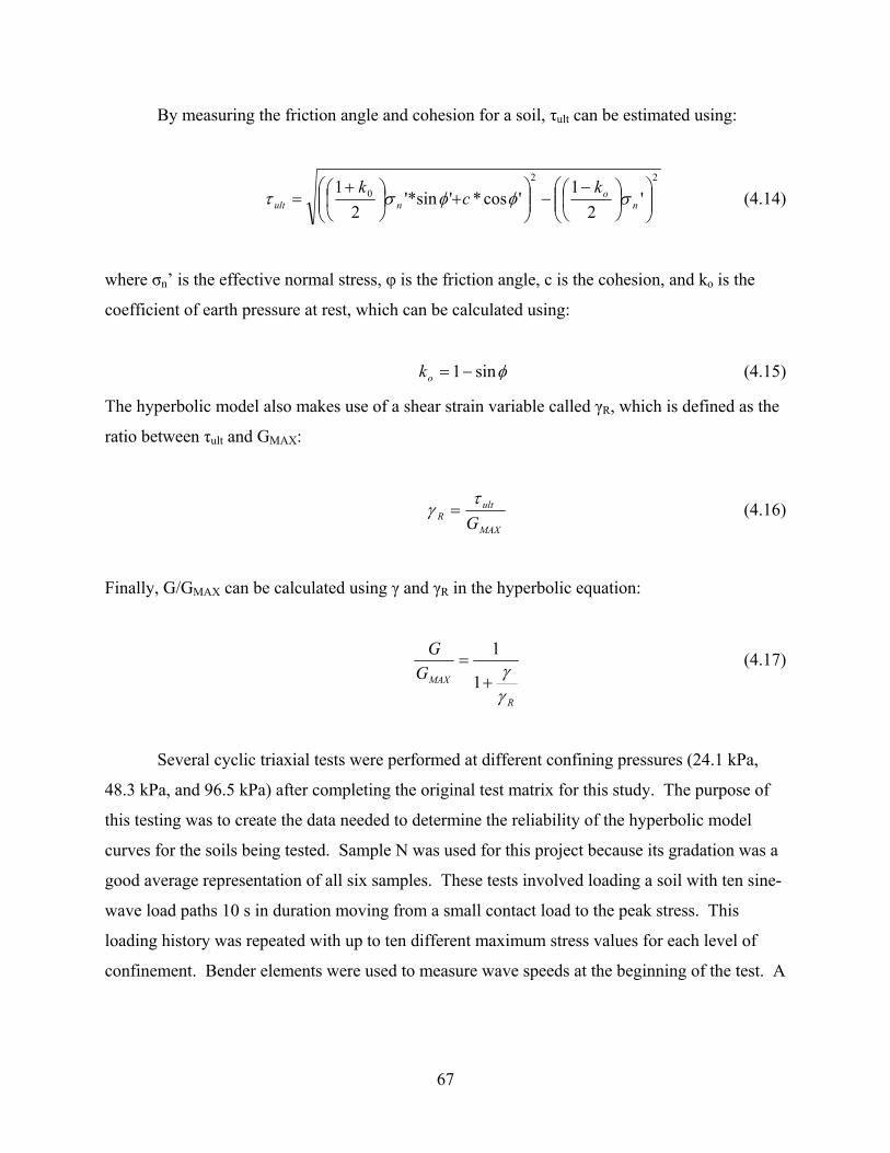
67
By measuring the friction angle and cohesion for a soil, τult can be estimated using:
220 '
21
'cos*'sin'*2
1
−
−
+
+
= no
nultk
ck
σφφστ (4.14)
where σn’ is the effective normal stress, φ is the friction angle, c is the cohesion, and ko is the
coefficient of earth pressure at rest, which can be calculated using:
φsin1−=ok (4.15)
The hyperbolic model also makes use of a shear strain variable called γR, which is defined as the
ratio between τult and GMAX:
MAX
ultR G
τγ = (4.16)
Finally, G/GMAX can be calculated using γ and γR in the hyperbolic equation:
R
MAXGG
γγ
+=
1
1 (4.17)
Several cyclic triaxial tests were performed at different confining pressures (24.1 kPa,
48.3 kPa, and 96.5 kPa) after completing the original test matrix for this study. The purpose of
this testing was to create the data needed to determine the reliability of the hyperbolic model
curves for the soils being tested. Sample N was used for this project because its gradation was a
good average representation of all six samples. These tests involved loading a soil with ten sine-
wave load paths 10 s in duration moving from a small contact load to the peak stress. This
loading history was repeated with up to ten different maximum stress values for each level of
confinement. Bender elements were used to measure wave speeds at the beginning of the test. A
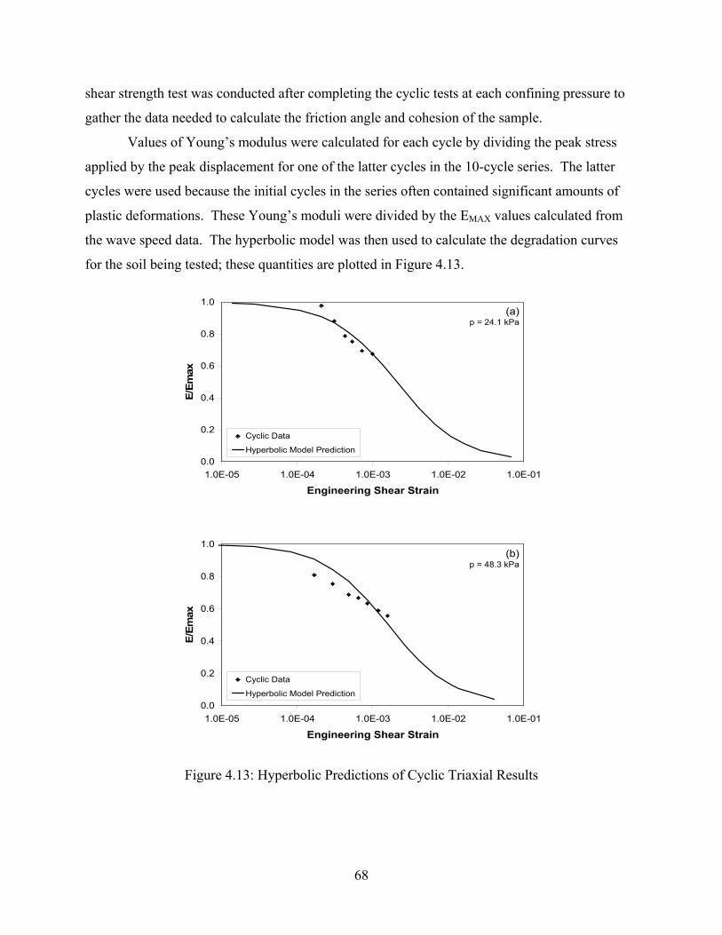
68
shear strength test was conducted after completing the cyclic tests at each confining pressure to
gather the data needed to calculate the friction angle and cohesion of the sample.
Values of Young’s modulus were calculated for each cycle by dividing the peak stress
applied by the peak displacement for one of the latter cycles in the 10-cycle series. The latter
cycles were used because the initial cycles in the series often contained significant amounts of
plastic deformations. These Young’s moduli were divided by the EMAX values calculated from
the wave speed data. The hyperbolic model was then used to calculate the degradation curves
for the soil being tested; these quantities are plotted in Figure 4.13.
0.0
0.2
0.4
0.6
0.8
1.0
1.0E-05 1.0E-04 1.0E-03 1.0E-02 1.0E-01
Engineering Shear Strain
E/Em
ax
Cyclic Data
Hyperbolic Model Prediction
(a)p = 24.1 kPa
0.0
0.2
0.4
0.6
0.8
1.0
1.0E-05 1.0E-04 1.0E-03 1.0E-02 1.0E-01
Engineering Shear Strain
E/Em
ax
Cyclic Data
Hyperbolic Model Prediction
(b)p = 48.3 kPa
Figure 4.13: Hyperbolic Predictions of Cyclic Triaxial Results

69
0.0
0.2
0.4
0.6
0.8
1.0
1.0E-05 1.0E-04 1.0E-03 1.0E-02 1.0E-01
Engineering Shear Strain
E/Em
ax
Cyclic Data
Hyperbolic Model Prediction
(c)p = 96.5 kPa
Figure 4.13 Continued: Hyperbolic Predictions of Cyclic Triaxial Results
The hyperbolic model predictions match the experimental data closely. The majority of
the cyclic triaxial data points are within 5% of the predicted values for that strain level. Some of
the points at the limits of each sequence differ from the predicted values by up to 15%.
However, many of the points at the smallest strain were calculated near the resolution limit of the
displacement measurements. In addition, α values for the points with the smallest strains were
relatively large compared to the other points as indicated by Table 4.3.
The hyperbolic model appears to predict a slightly steeper E/EMAX slope than the data
would suggest over the strain region being tested. The cause for this is unknown. However, if
the curves suggested by the cyclic triaxial data trends were extended they would not reach an
E/EMAX value of 1.0 at a strain level of 0.001%. As stated in section 2.2.3, most researchers
agree that sandy soils are within the linear region of the stress-strain curve below this strain
threshold. Based on these observations the hyperbolic model appears to provide a good fit for
the experimental data.
70
Chapter 5 Summary and Conclusions
This study involved a comparative resilient modulus and bender element testing of 36 triaxial
specimens. Six granular soils representative of base and subgrade materials found in Minnesota
were used. These specimens were prepared at three different moisture contents per soil and
compacted to their standard Proctor optimum dry density. Each specimen was subjected to
resilient modulus testing as specified by Mn/DOT modified LTPP P46. The loading sequences
of this test were halted periodically to perform small strain bender element testing, which can
establish relative maximum modulus values by measuring wave speeds. Following the test
protocol, the specimens were loaded until failure to determine their shear strength. The objective
of this testing was to measure the resilient modulus values of reference soil samples while
establishing a relationship between the resilient modulus and the maximum modulus of these
soils. A number of conclusions were reached during this investigation.
1) The hyperbolic model is able to accurately model the strain-dependent modulus reduction of
a soil using only the small-strain modulus, friction angle, and cohesion as input parameters. As a
result, the maximum modulus values calculated from the wave speeds measured by small strain
testing instruments can be converted into resilient modulus values knowing only the cohesion
and friction angle of the soil. The cohesion and friction angle of the soil can be established
during shear strength testing. Therefore, pavement inspectors can use this relation to relate the
results of the small-strain testing instruments used in the field to the laboratory-measured
resilient modulus values used in pavement design.
2) The modulus and strength of soils tested increased as their moisture contents decreased. This
trend was visible in the results from the resilient modulus, bender element, and triaxial strength
testing. This is a reasonable result that is consistent with the large amount of energy used to
compact the specimens with smaller moisture contents.
71
3) The three LVDTs used as a part of the triaxial testing setup often measured displacement
values that were in poor agreement with each other. Possible causes for this include uneven
specimen deformation, an uneven specimen surface, or a poor bond between the LVDT
apparatus and the specimens’ membranes. A quantity called an α-value was used to model the
degree to which the displacement measures were inconsistent for each loading sequence of each
test. Loading sequences performed with relatively low deviator stresses had larger α-values than
the other tests.
4) The best estimate of the gravimetric moisture content from the dielectric permittivity values
in this study is
However, this relation often produces moisture content differences of 0.03 to 4.63 percent from
the oven dried values, and is unproven for soils other than the six used in this study.
47.318.1 −= kω
72
References [1] Hoffmann, O. Verification and Enhancements of Portable Deflectometer Devices
(Minneapolis, MN.: University of Minnesota, 2003). [2] Federal Highway Administration Pavement Performance Division, Resilient Modulus of
Unbound Granular Base/Subbase Materials and Subgrade Soils, Long Term Pavement Performance, Protocol 46 (Federal Highway Administration Pavement Performance Division, 1996).
[3] National Cooperative Highway Research Program, Recommended Standard Method for
Routine Resilient Modulus Testing of Unbound Granular Base/Subbase Materials and Subgrade Soils, Protocol 1-28A (National Cooperative Highway Research Program, 2002).
[4] Atkinson, J.H. and Sallfors, G. (1991). Exerimental determination of stress-strain-time
characteristics in laboratory and in situ tests. Proceedings of the International Conference on Soil Mechanics and Foundation Engineering, V3: 915-956.
[5] Lai, C. G. and Rix, G. J. (2002). Solution of the Rayleigh Eigenproblem in Viscoelastic
Materials. Bulletin of the Seismological Society of America, V92(6): 2297- 2309. [6] Tatsuoka, F., Teachavorasinskun, S., Dong, J., Kohata, Y., and Sato T. (1994).
Importance of measuring local strains in cyclic triaxial tests on granular materials. ASTM Special Technical Publication, No. 1213: 288-302.
[7] Cuccovillo, T. and Coop, M.R. (1997). The measurement of local axial strains in triaxial
tests using LVDTs. Geotechnique, V47(1): 167-171. [8] Jovicic, V. and Coop, M.R. (1997). Stiffness of coarse-grained soils at small strains.
Geotechnique, V47(3): 545-561. [9] Iwasaki, T., Tatsuoka, F., and Takagi, Y. (1978). Shear moduli of sands under cyclic
torsional shear loading. Soils and Foundations, V18(1): 39-56. [10] Bolton, M.D. and Wilson, J.M.R. (1989). Experimental and theoretical comparison
between static and dynamic torsional soil tests. Geotechnique, V39(4): 585-599. [11] Jovicic, V. and Coop, M.R. (1998). The measurement of stiffness anisotropy in clays
with bender element tests in the triaxial apparatus. Geotechnical Testing Journal, V21(1): 3-10.
[12] Jovicic, V. and Coop, M.R. (1996). Objective criteria for determining Gmax from bender
element tests. Geotechnique, V46(2): 357-362.

73
[13] Schmertmann, J. H. (1991). The mechanical aging of soils. The twenty-fifth Karl
Terzaghi lecture. Journal of Geotechnical Engineering, ASCE, V105(9): 1288-1330. [14] Santamarina, J.C. and Fratta, D. (1998). Introduction to Discrete Signals and Inverse
Problems in Civil Engineering. ASCE Press, Reston, VA: 63-71. [15] Ishibashi, I. (1992). Discussion to “Effect of soil plasticity on cyclic response”. Journal of Geotechnical Engineering, V118(5): 830-832. [16] Sanches-Salinero, I., Roesset, J. M.and Stokoe, K. H. . Analytical studies of body wave
propagation and attenuation (Austin, TX.: University of Texas, Report GR 86-15, 1986). [17] Viggiani, G. and Atkinson, J.H. (1995). Interpretation of bender element tests.
Geotechnique, V45(1): 149-154.
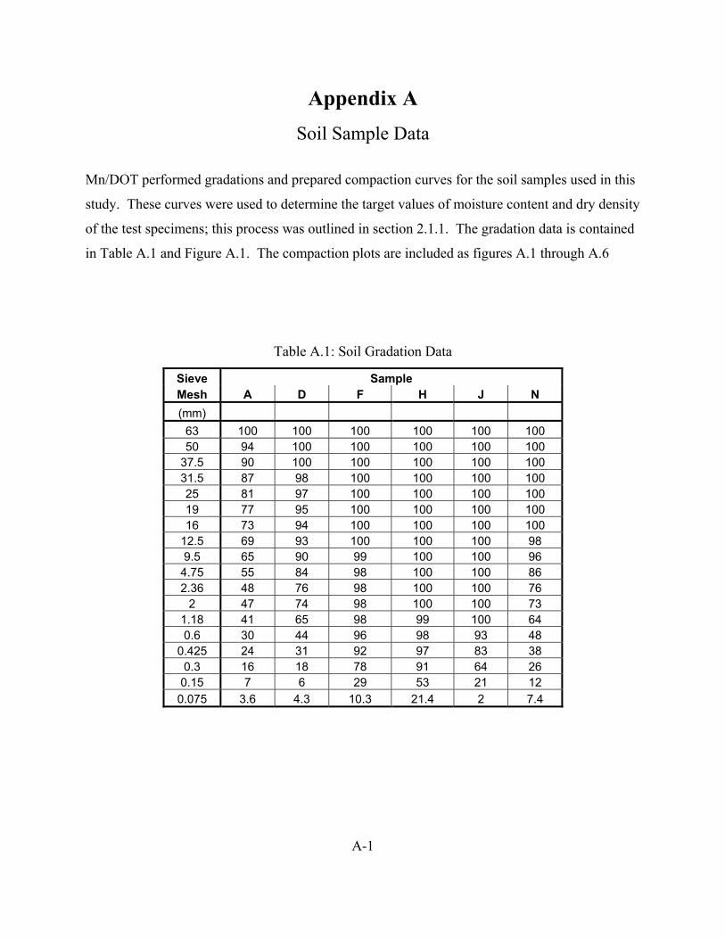
A-1
Appendix A Soil Sample Data
Mn/DOT performed gradations and prepared compaction curves for the soil samples used in this
study. These curves were used to determine the target values of moisture content and dry density
of the test specimens; this process was outlined in section 2.1.1. The gradation data is contained
in Table A.1 and Figure A.1. The compaction plots are included as figures A.1 through A.6
Table A.1: Soil Gradation Data Sieve Sample Mesh A D F H J N (mm)
63 100 100 100 100 100 100 50 94 100 100 100 100 100
37.5 90 100 100 100 100 100 31.5 87 98 100 100 100 100 25 81 97 100 100 100 100 19 77 95 100 100 100 100 16 73 94 100 100 100 100
12.5 69 93 100 100 100 98 9.5 65 90 99 100 100 96
4.75 55 84 98 100 100 86 2.36 48 76 98 100 100 76
2 47 74 98 100 100 73 1.18 41 65 98 99 100 64 0.6 30 44 96 98 93 48
0.425 24 31 92 97 83 38 0.3 16 18 78 91 64 26
0.15 7 6 29 53 21 12 0.075 3.6 4.3 10.3 21.4 2 7.4
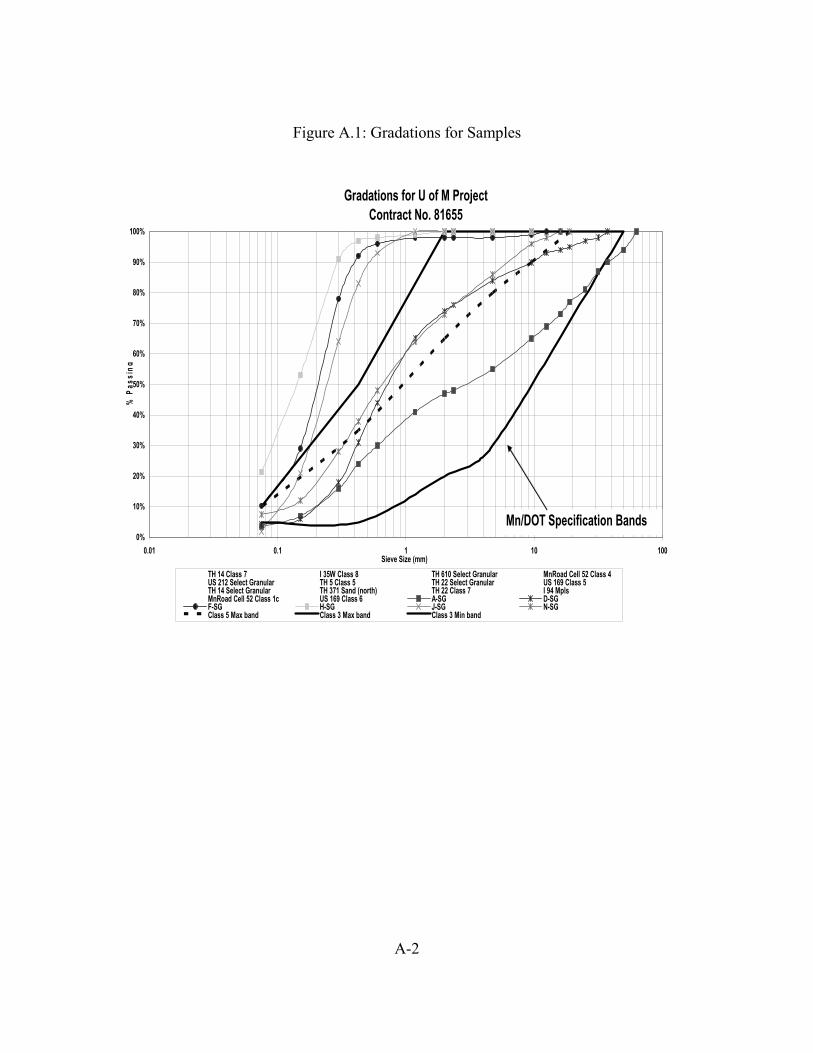
A-2
Figure A.1: Gradations for Samples
Gradations for U of M ProjectContract No. 81655
0%
10%
20%
30%
40%
50%
60%
70%
80%
90%
100%
0.01 0.1 1 10 100Sieve Size (mm)
% P
assi
ng
TH 14 Class 7 I 35W Class 8 TH 610 Select Granular MnRoad Cell 52 Class 4US 212 Select Granular TH 5 Class 5 TH 22 Select Granular US 169 Class 5TH 14 Select Granular TH 371 Sand (north) TH 22 Class 7 I 94 MplsMnRoad Cell 52 Class 1c US 169 Class 6 A-SG D-SGF-SG H-SG J-SG N-SGClass 5 Max band Class 3 Max band Class 3 Min band
Mn/DOT Specification Bands

A-3
Figure A.2: Standard Proctor Compaction Curve for Sample A
Figure A.3: Standard Proctor Compaction Curve for Sample D
1900
2000
2100
2200
0% 5% 10% 15%
Moisture Content
Dry
Den
sity
(kg/
m3)
Optimum Moisture Content = 7.9%Maxiumum Dry Unit Weight = 2158 kg/m3
1600
1700
1800
1900
0% 5% 10% 15%
Moisture Content
Dry
Den
sity
(kg/
m3)
Optimum Moisture Content = 10.0%Maxiumum Dry Unit Weight = 1839 kg/m3

A-4
Figure A.4: Standard Proctor Compaction Curve for Sample F
Figure A.5: Standard Proctor Compaction Curve for Sample H
1700
1800
1900
2000
0% 5% 10% 15%
Moisture Content
Dry
Den
sity
(kg/
m3)
Optimum Moisture Content = 9.3%Maxiumum Dry Unit Weight = 1900 kg/m3
1500
1600
1700
1800
0% 5% 10% 15%
Moisture Content
Dry
Den
sity
(kg/
m3)
Optimum Moisture Content = 12.6%Maxiumum Dry Unit Weight = 1725 kg/m3
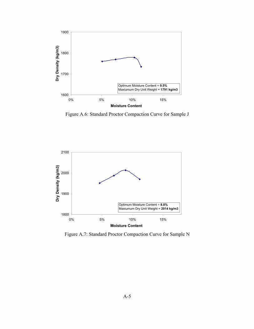
A-5
Figure A.6: Standard Proctor Compaction Curve for Sample J
Figure A.7: Standard Proctor Compaction Curve for Sample N
1600
1700
1800
1900
0% 5% 10% 15%
Moisture Content
Dry
Den
sity
(kg/
m3)
Optimum Moisture Content = 9.5%Maxiumum Dry Unit Weight = 1791 kg/m3
1800
1900
2000
2100
0% 5% 10% 15%
Moisture Content
Dry
Den
sity
(kg/
m3)
Optimum Moisture Content = 8.8%Maxiumum Dry Unit Weight = 2014 kg/m3
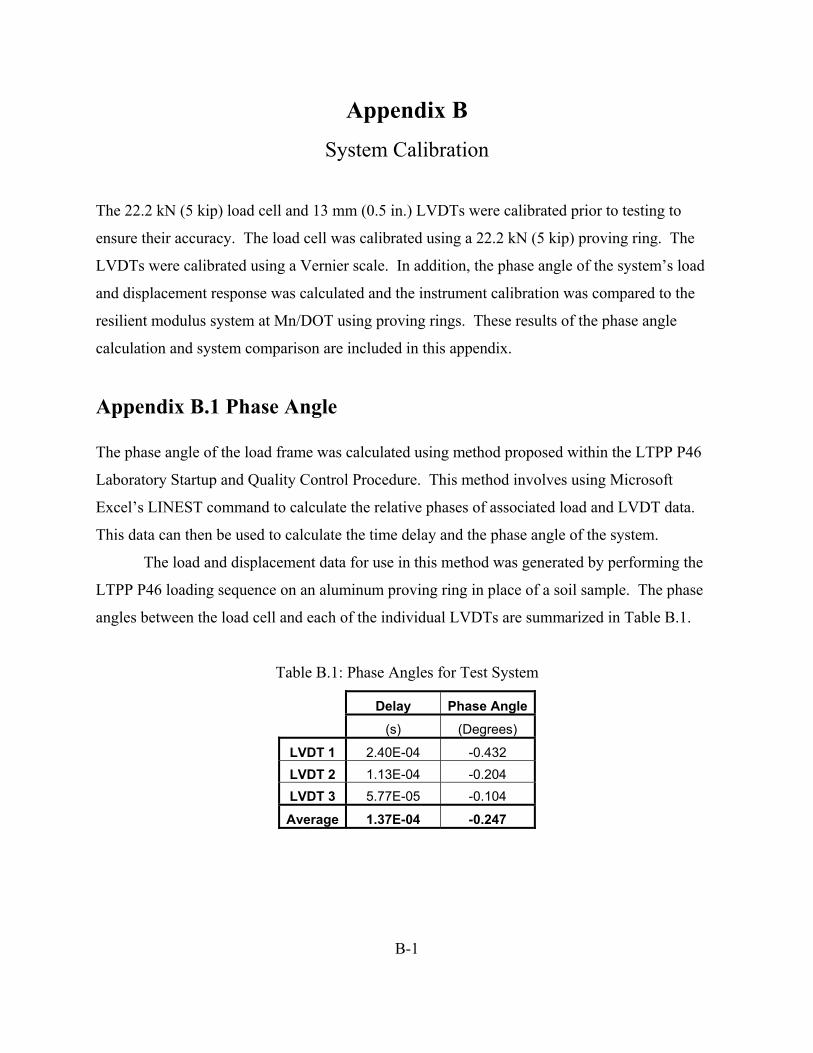
B-1
Appendix B System Calibration
The 22.2 kN (5 kip) load cell and 13 mm (0.5 in.) LVDTs were calibrated prior to testing to
ensure their accuracy. The load cell was calibrated using a 22.2 kN (5 kip) proving ring. The
LVDTs were calibrated using a Vernier scale. In addition, the phase angle of the system’s load
and displacement response was calculated and the instrument calibration was compared to the
resilient modulus system at Mn/DOT using proving rings. These results of the phase angle
calculation and system comparison are included in this appendix.
Appendix B.1 Phase Angle
The phase angle of the load frame was calculated using method proposed within the LTPP P46
Laboratory Startup and Quality Control Procedure. This method involves using Microsoft
Excel’s LINEST command to calculate the relative phases of associated load and LVDT data.
This data can then be used to calculate the time delay and the phase angle of the system.
The load and displacement data for use in this method was generated by performing the
LTPP P46 loading sequence on an aluminum proving ring in place of a soil sample. The phase
angles between the load cell and each of the individual LVDTs are summarized in Table B.1.
Table B.1: Phase Angles for Test System
Delay Phase Angle
(s) (Degrees)
LVDT 1 2.40E-04 -0.432 LVDT 2 1.13E-04 -0.204 LVDT 3 5.77E-05 -0.104
Average 1.37E-04 -0.247
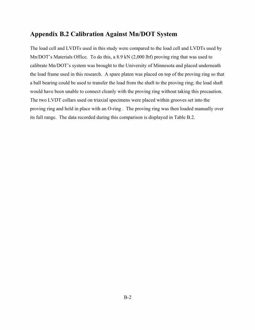
B-2
Appendix B.2 Calibration Against Mn/DOT System
The load cell and LVDTs used in this study were compared to the load cell and LVDTs used by
Mn/DOT’s Materials Office. To do this, a 8.9 kN (2,000 lbf) proving ring that was used to
calibrate Mn/DOT’s system was brought to the University of Minnesota and placed underneath
the load frame used in this research. A spare platen was placed on top of the proving ring so that
a ball bearing could be used to transfer the load from the shaft to the proving ring; the load shaft
would have been unable to connect cleanly with the proving ring without taking this precaution.
The two LVDT collars used on triaxial specimens were placed within grooves set into the
proving ring and held in place with an O-ring . The proving ring was then loaded manually over
its full range. The data recorded during this comparison is displayed in Table B.2.
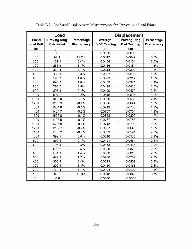
B-3
Table B.2. Load and Displacement Measurements for University’s Load Frame
Load Displacement Triaxial Proving Ring Percentage Average Proving Ring Percentage
Load Cell Calculated Discrepancy LVDT Reading Dial Reading Discrepancy(lb) (lb) (in) (in) 10 0.0 - 0.0000 0.0000 -
100 89.1 12.2% 0.0049 0.0047 3.5% 200 189.8 5.4% 0.0104 0.0101 2.6% 300 285.6 5.1% 0.0156 0.0154 1.3% 400 389.3 2.7% 0.0213 0.0209 1.8% 500 488.8 2.3% 0.0267 0.0262 1.9% 600 590.7 1.6% 0.0323 0.0317 1.8% 700 693.2 1.0% 0.0379 0.0371 2.1% 800 795.7 0.5% 0.0435 0.0426 2.0% 900 896.4 0.4% 0.0490 0.0479 2.2% 1000 997.7 0.2% 0.0545 0.0535 1.9% 1100 1099.0 0.1% 0.0600 0.0588 2.1% 1200 1200.9 -0.1% 0.0656 0.0644 1.9% 1300 1304.6 -0.4% 0.0713 0.0700 1.8% 1400 1404.7 -0.3% 0.0767 0.0754 1.8% 1500 1506.0 -0.4% 0.0823 0.0809 1.7% 1400 1403.5 -0.2% 0.0767 0.0753 1.8% 1300 1305.8 -0.4% 0.0713 0.0700 1.9% 1200 1202.7 -0.2% 0.0657 0.0645 1.9% 1100 1103.2 -0.3% 0.0603 0.0591 2.0% 1000 999.5 0.0% 0.0546 0.0535 2.1% 900 899.4 0.1% 0.0491 0.0481 2.1% 800 793.3 0.8% 0.0433 0.0425 2.0% 700 696.2 0.5% 0.0380 0.0372 2.2% 600 591.9 1.4% 0.0323 0.0316 2.3% 500 494.3 1.2% 0.0270 0.0264 2.3% 400 390.5 2.4% 0.0213 0.0208 2.6% 300 290.5 3.3% 0.0159 0.0155 2.4% 200 189.8 5.4% 0.0104 0.0102 1.6% 100 88.5 13.0% 0.0048 0.0048 0.7% 10 -0.6 - 0.0000 -0.0001 -
B-4
The University of Minnesota’s load frame produced results in good agreement with
Mn/DOT’s proving ring. The load readings were within 1% of the proving ring’s value for the
majority of its range; the less accurate readings at low load levels were the result of seating. The
average LVDT displacement readings were consistently about 2% larger than the displacements
measured by the dial gage of the proving ring.
One of the University of Minnesota’s 8.9 kN (2 kip) proving rings was loaded inside of
Mn/DOT load frame, however, due to an incompatible LVDT attachment system the
displacement of the proving ring could not be recorded. The load data recorded during this test
is displayed in Table B.3.
Table B.3. Load Measurements for Mn/DOT’s Load Frame
Load Triaxial Proving Ring Percentage
Load Cell Calculated Discrepancy (lb) (lb) 9.0 14.7 -
244.9 239.7 2.2% 491.5 488.1 0.7% 736.4 729.8 0.9% 982.9 981.2 0.2% 886.3 893.1 -0.8% 788.0 796.3 -1.0% 689.7 700.4 -1.5% 589.8 600.6 -1.8% 491.5 497.9 -1.3% 393.2 403.0 -2.4% 294.9 304.2 -3.1% 244.9 252.4 -3.0% 195.0 206.4 -5.5% 95.1 102.7 -7.4% 6.5 18.6 -65.3%

B-5
The maximum load tested within the Mn/DOT load frame was lower than the maximum
load tested within the load frame used for this research due to concerns about the stability of the
proving ring within the system. However, the existing data indicates
that both systems have similar contact problems at small loads and similar success measuring
loads above 2.22 kN (500 lbf). The one noticeable difference between the systems was that the
Mn/DOT system overestimated the load on the return section of the test while the load frame
used during this research underestimated it by a similar amount. However, the load values
measured during resilient modulus testing were taken at peaks
and during rest periods between pulses; the data recorded by both systems should be comparable
at these times.
The resilient modulus test is dynamic, therefore, an extra test was performed to determine
whether both load frames would determine the same resilient modulus for the same material.
This comparison would be impossible to carry out on a soil specimen without damaging the soil,
therefore, the resilient modulus test regimen was carried out on a proving ring. The modulus
calculated from a test of a proving ring would have little physical meaning, however, it would
serve to compare systems. After performing a resilient modulus test procedure on a proving ring
using both load frames the calculated MR values were within 5% of each other.
It is reasonable to assume, based upon the data presented in this section, that the
University of Minnesota’s load frame would produce results comparable to the results from
Mn/DOT’s load frame.

C-1
Appendix C Resilient Modulus Data Calculation Program
The following MATLAB 5.3 program was written to convert the data files produced during
resilient modulus testing into a matrix containing load, displacement, stress, strain, and modulus
data. The 15 data files produced during the resilient modulus testing are named Cycle1, Cycle2,
etc. The program is run once for each of these cycles & the data from each is automatically
placed into a spreadsheet within the MATLAB folder. The calculations take place using English
units.
************************************************************************ % Load Cycle number 'i' clear; load Data.txt; N = Data; load Cyclei; M = Cyclei; O = i; % Confining Pressure of Cycle 'i' = 'j' N(((((O-1)*5)+1):(((O-1)*5)+5)), 1) = j; % Location of first load peak = 'k' y = k; % Set location to begin local maxima search y = y - 100; % Reset variables count = 1; W = 0; X = 0; Y = 0; Z = 0; % Search for load/displacement peaks
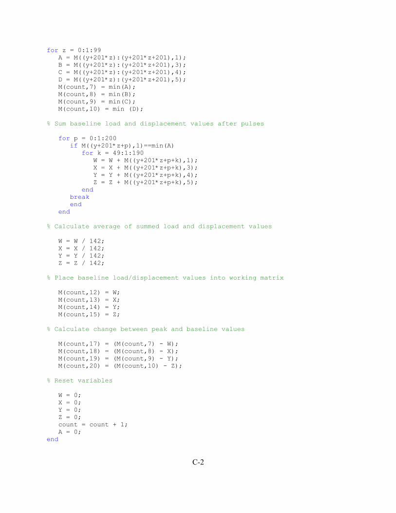
C-2
for z = 0:1:99 A = M((y+201*z):(y+201*z+201),1); B = M((y+201*z):(y+201*z+201),3); C = M((y+201*z):(y+201*z+201),4); D = M((y+201*z):(y+201*z+201),5); M(count,7) = min(A); M(count,8) = min(B); M(count,9) = min(C); M(count,10) = min (D); % Sum baseline load and displacement values after pulses for p = 0:1:200 if M((y+201*z+p),1)==min(A) for k = 49:1:190 W = W + M((y+201*z+p+k),1); X = X + M((y+201*z+p+k),3); Y = Y + M((y+201*z+p+k),4); Z = Z + M((y+201*z+p+k),5); end break end end % Calculate average of summed load and displacement values W = W / 142; X = X / 142; Y = Y / 142; Z = Z / 142; % Place baseline load/displacement values into working matrix M(count,12) = W; M(count,13) = X; M(count,14) = Y; M(count,15) = Z; % Calculate change between peak and baseline values M(count,17) = (M(count,7) - W); M(count,18) = (M(count,8) - X); M(count,19) = (M(count,9) - Y); M(count,20) = (M(count,10) - Z); % Reset variables W = 0; X = 0; Y = 0; Z = 0; count = count + 1; A = 0; end
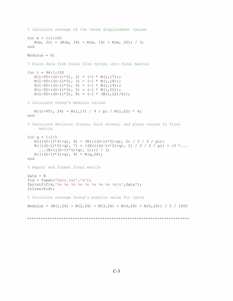
C-3
% Calculate average of the three displacement values for m = 1:1:100 M(m, 22) = (M(m, 18) + M(m, 19) + M(m, 20)) / 3; end Modulus = 0; % Place data from final five cycles into final matrix for l = 96:1:100 N(l-95+((O-1)*5), 2) = (-1 * M(l,17)); N(l-95+((O-1)*5), 3) = (-1 * M(l,18)); N(l-95+((O-1)*5), 4) = (-1 * M(l,19)); N(l-95+((O-1)*5), 5) = (-1 * M(l,20)); N(l-95+((O-1)*5), 8) = (-1 * (M(l,22)/6)); % Calculate Young's modulus values M((l-95), 24) = M(l,17) / 9 / pi / M(l,22) * 6; end % Calculate deviator stress, bulk stress, and place values in final matrix for q = 1:1:5 N((((O-1)*5)+q), 6) = (N((((O-1)*5)+q), 2) / 3 / 3 / pi); N((((O-1)*5)+q), 7) = ((N((((O-1)*5)+q), 2) / 3 / 3 / pi) + (3 *... ...(N((((O-1)*5)+q), 1)))) / 3; N((((O-1)*5)+q), 9) = M(q,24); end % Export and format final matrix Data = N fid = fopen('Data.txt','w'); fprintf(fid,'%e %e %e %e %e %e %e %e %e\n',Data'); fclose(fid); % Calculate average Young's modulus value for cycle Modulus = (M(1,24) + M(2,24) + M(3,24) + M(4,24) + M(5,24)) / 5 / 1000 ***********************************************************************
D-1
Appendix D Data
Two of the most interesting ways to plot the resilient modulus and bender element data from this
study are on plots using the Young’s modulus versus confining pressure. This appendix contains
these plots for each sample at every moisture content tested. The data from both repeats are
included on the plot; the trendlines are created using the average of the data from both. Section
D.1 contains the comparisons between the resilient modulus and EMAX; section D.2 contains the
comparisons between the resilient modulus and confining pressure.
D.1 Resilient Modulus and EMAX Versus Confining Pressure
One of the primary goals of this research was to formulate a correlation between the resilient
modulus and EMAX. Figures D.1 through D.6 display data from both of these variables plotted
against the confining pressure.
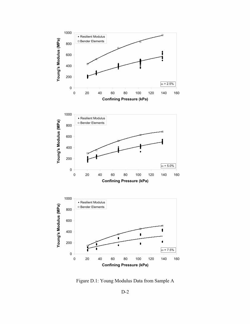
D-2
Figure D.1: Young Modulus Data from Sample A
0
200
400
600
800
1000
0 20 40 60 80 100 120 140 160
Confining Pressure (kPa)
Youn
g's
Mod
ulus
(MPa
) Resilient ModulusBender Elements
ω = 2.5%
0
200
400
600
800
1000
0 20 40 60 80 100 120 140 160
Confining Pressure (kPa)
Youn
g's
Mod
ulus
(MPa
) Resilient ModulusBender Elements
ω = 5.0%
0
200
400
600
800
1000
0 20 40 60 80 100 120 140 160
Confining Pressure (kPa)
Youn
g's
Mod
ulus
(MPa
) Resilient ModulusBender Elements
ω = 7.5%
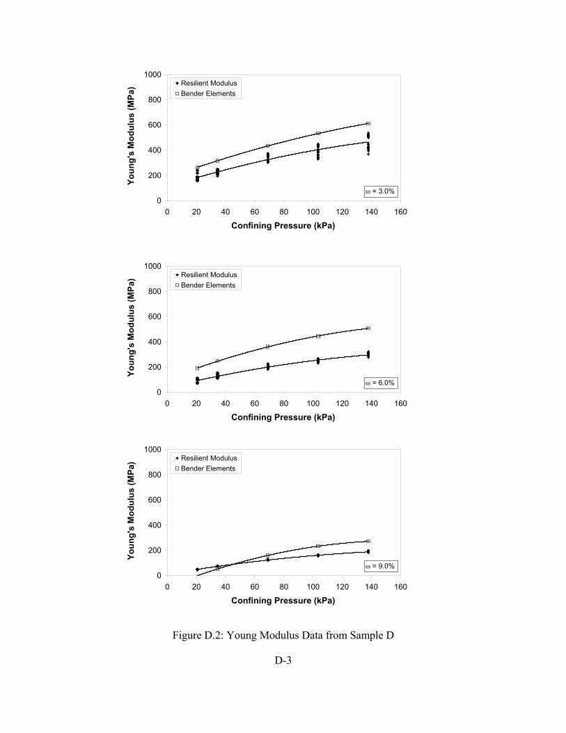
D-3
Figure D.2: Young Modulus Data from Sample D
0
200
400
600
800
1000
0 20 40 60 80 100 120 140 160
Confining Pressure (kPa)
Youn
g's
Mod
ulus
(MPa
) Resilient ModulusBender Elements
ω = 3.0%
0
200
400
600
800
1000
0 20 40 60 80 100 120 140 160
Confining Pressure (kPa)
Youn
g's
Mod
ulus
(MPa
) Resilient ModulusBender Elements
ω = 6.0%
0
200
400
600
800
1000
0 20 40 60 80 100 120 140 160
Confining Pressure (kPa)
Youn
g's
Mod
ulus
(MPa
) Resilient ModulusBender Elements
ω = 9.0%
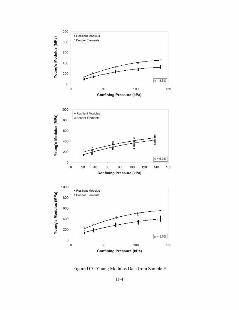
D-4
Figure D.3: Young Modulus Data from Sample F
0
200
400
600
800
1000
0 50 100 150
Confining Pressure (kPa)
Youn
g's
Mod
ulus
(MPa
) Resilient ModulusBender Elements
ω = 3.5%
0
200
400
600
800
1000
0 20 40 60 80 100 120 140 160
Confining Pressure (kPa)
Youn
g's
Mod
ulus
(MPa
) Resilient ModulusBender Elements
ω = 6.0%
0
200
400
600
800
1000
0 50 100 150
Confining Pressure (kPa)
Youn
g's
Mod
ulus
(MPa
) Resilient ModulusBender Elements
ω = 8.5%

D-5
Figure D.4: Young Modulus Data from Sample H
0
200
400
600
800
1000
0 50 100 150
Confining Pressure (kPa)
Youn
g's
Mod
ulus
(MPa
) Resilient ModulusBender Elements
ω = 3.0%
0
200
400
600
800
1000
0 50 100 150
Confining Pressure (kPa)
Youn
g's
Mod
ulus
(MPa
) Resilient ModulusBender Elements
ω = 7.0%
0
200
400
600
800
1000
0 50 100 150
Confining Pressure (kPa)
Youn
g's
Mod
ulus
(MPa
) Resilient ModulusBender Elements
ω = 11.0%
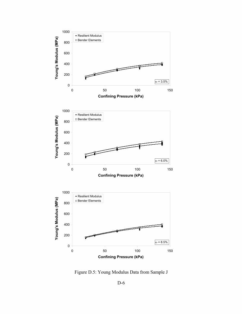
D-6
Figure D.5: Young Modulus Data from Sample J
0
200
400
600
800
1000
0 50 100 150
Confining Pressure (kPa)
Youn
g's
Mod
ulus
(MPa
) Resilient ModulusBender Elements
ω = 3.5%
0
200
400
600
800
1000
0 50 100 150
Confining Pressure (kPa)
Youn
g's
Mod
ulus
(MPa
) Resilient ModulusBender Elements
ω = 6.0%
0
200
400
600
800
1000
0 50 100 150
Confining Pressure (kPa)
Youn
g's
Mod
ulus
(MPa
) Resilient ModulusBender Elements
ω = 8.5%
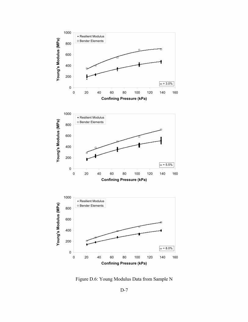
D-7
Figure D.6: Young Modulus Data from Sample N
0
200
400
600
800
1000
0 20 40 60 80 100 120 140 160
Confining Pressure (kPa)
Youn
g's
Mod
ulus
(MPa
) Resilient ModulusBender Elements
ω = 3.0%
0
200
400
600
800
1000
0 20 40 60 80 100 120 140 160
Confining Pressure (kPa)
Youn
g's
Mod
ulus
(MPa
) Resilient ModulusBender Elements
ω = 5.5%
0
200
400
600
800
1000
0 20 40 60 80 100 120 140 160
Confining Pressure (kPa)
Youn
g's
Mod
ulus
(MPa
) Resilient ModulusBender Elements
ω = 8.0%
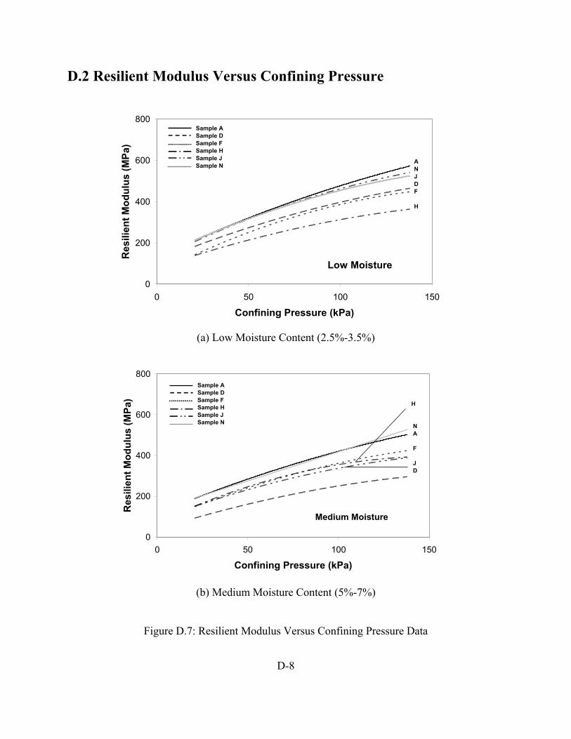
D-8
D.2 Resilient Modulus Versus Confining Pressure
0
200
400
600
800
0 50 100 150
Confining Pressure (kPa)
Res
ilien
t Mod
ulus
(MPa
)Sample ASample DSample FSample HSample JSample N
A N J D F
H
Low Moisture
(a) Low Moisture Content (2.5%-3.5%)
0
200
400
600
800
0 50 100 150
Confining Pressure (kPa)
Res
ilien
t Mod
ulus
(MPa
)
Sample ASample DSample FSample HSample JSample N
H
N A
F
J D
Medium Moisture
(b) Medium Moisture Content (5%-7%)
Figure D.7: Resilient Modulus Versus Confining Pressure Data
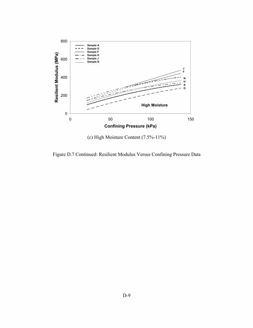
D-9
0
200
400
600
800
0 50 100 150
Confining Pressure (kPa)
Res
ilien
t Mod
ulus
(MPa
)
Sample ASample DSample FSample HSample JSample N
J F
N H A D
High Moisture
(c) High Moisture Content (7.5%-11%)
Figure D.7 Continued: Resilient Modulus Versus Confining Pressure Data

D-10
D.3 Resilient Modulus Versus Mean Stress
The mean stress is another quantity that was calculated during this study. Figures D.8 to D.13
plot the resilient modulus against the mean stress against the confining for each sample and
moisture content.

D-11
Figure D.8: Resilient Modulus and Mean Stress Data from Sample A
0
200
400
600
800
1000
0 50 100 150 200 250
Mean Stress (kPa)
Res
ilien
t Mod
ulus
(MPa
)
ω = 2.5%
0
200
400
600
800
1000
0 50 100 150 200 250
Mean Stress (kPa)
Res
ilien
t Mod
ulus
(MPa
)
ω = 5.0%
0
200
400
600
800
1000
0 50 100 150 200 250
Mean Stress (kPa)
Res
ilien
t Mod
ulus
(MPa
)
ω = 7.5%
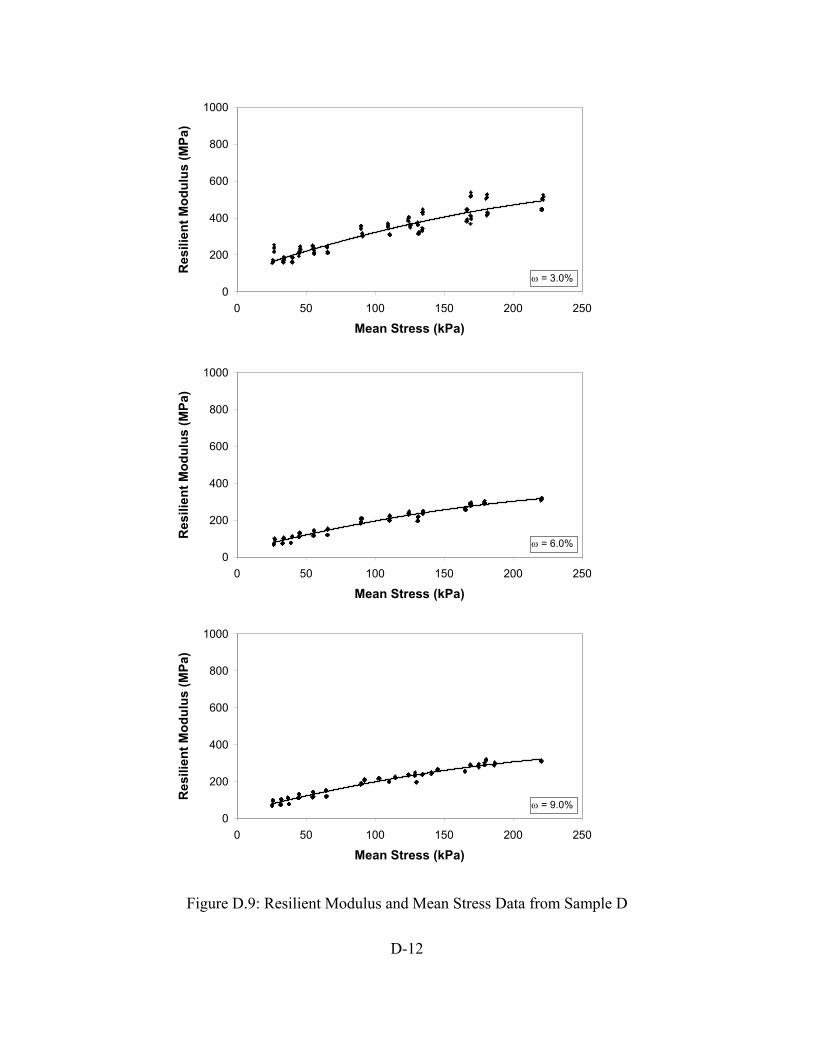
D-12
Figure D.9: Resilient Modulus and Mean Stress Data from Sample D
0
200
400
600
800
1000
0 50 100 150 200 250
Mean Stress (kPa)
Res
ilien
t Mod
ulus
(MPa
)
ω = 3.0%
0
200
400
600
800
1000
0 50 100 150 200 250
Mean Stress (kPa)
Res
ilien
t Mod
ulus
(MPa
)
ω = 6.0%
0
200
400
600
800
1000
0 50 100 150 200 250
Mean Stress (kPa)
Res
ilien
t Mod
ulus
(MPa
)
ω = 9.0%

D-13
Figure D.10: Resilient Modulus and Mean Stress Data from Sample F
0
200
400
600
800
1000
0 50 100 150 200 250
Mean Stress (kPa)
Res
ilien
t Mod
ulus
(MPa
)
ω = 3.5%
0
200
400
600
800
1000
0 50 100 150 200 250
Mean Stress (kPa)
Res
ilien
t Mod
ulus
(MPa
)
ω = 6.0%
0
200
400
600
800
1000
0 50 100 150 200 250
Mean Stress (kPa)
Res
ilien
t Mod
ulus
(MPa
)
ω = 8.5%

D-14
Figure D.11: Resilient Modulus and Mean Stress Data from Sample H
0
200
400
600
800
1000
0 50 100 150 200 250
Mean Stress (kPa)
Res
ilien
t Mod
ulus
(MPa
)
ω = 3.0%
0
200
400
600
800
1000
0 50 100 150 200 250
Mean Stress (kPa)
Res
ilien
t Mod
ulus
(MPa
)
ω = 7.0%
0
200
400
600
800
1000
0 50 100 150 200 250
Mean Stress (kPa)
Res
ilien
t Mod
ulus
(MPa
)
ω = 11.0%
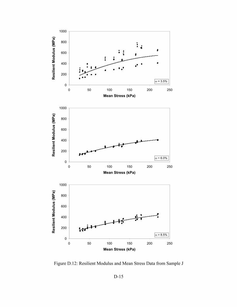
D-15
Figure D.12: Resilient Modulus and Mean Stress Data from Sample J
0
200
400
600
800
1000
0 50 100 150 200 250
Mean Stress (kPa)
Res
ilien
t Mod
ulus
(MPa
)
ω = 3.5%
0
200
400
600
800
1000
0 50 100 150 200 250
Mean Stress (kPa)
Res
ilien
t Mod
ulus
(MPa
)
ω = 6.0%
0
200
400
600
800
1000
0 50 100 150 200 250
Mean Stress (kPa)
Res
ilien
t Mod
ulus
(MPa
)
ω = 8.5%

D-16
Figure D.13: Resilient Modulus and Mean Stress Data from Sample N
0
200
400
600
800
1000
0 50 100 150 200 250
Mean Stress (kPa)
Res
ilien
t Mod
ulus
(MPa
)
ω = 3.0%
0
200
400
600
800
1000
0 50 100 150 200 250
Mean Stress (kPa)
Res
ilien
t Mod
ulus
(MPa
)
ω = 5.5%
0
200
400
600
800
1000
0 50 100 150 200 250
Mean Stress (kPa)
Res
ilien
t Mod
ulus
(MPa
)
ω = 8.0%
E-1
Appendix E MR Protocol Comparison
AASHTO’s LTPP P46 was used to direct the resilient modulus testing performed during this
study. However, a new resilient modulus test protocol entitled NCHRP 1-28A was released in
2002 with revised procedure as stated in section 2.1. One resilient modulus test was carried out
using the standard equipment for this study within the new protocol to establish that the
individual MR values recorded during the tests are similar. This appendix contains an itemized
test procedure as well as the results of the protocol comparison.
E.1 Itemized Test Procedure (LTPP P46)
1. Pour one 50 lb bag of the sample to be tested (there are three bags per sample) into a large container. Mix until homogeneous. 2. Determine the amount of soil and water to be mixed for the sample using the equations provided in Attachment A of LTPP P46. 3. Mix the correct amount of water and soil until the moisture content of the sample is relatively homogeneous. Take a moisture content sample from several locations within the sample; place this sample within an oven at approximately 125 degrees Fahrenheit. 4. Seal the remainder of the sample in an airtight container and allow it to temper overnight. 5. Before compaction remove the dry moisture content sample, calculate the moisture content of the sample, and adjust if necessary. Take three moisture content samples from the soil. 6. Inspect the base unit, mold, and top and bottom platens for damage and cleanliness. Place the porous stone on top of the platen and bender element if not already in place. 7. Attach a membrane to the lower bender element platen using two O-rings in the appropriate grooves. A third O-ring may be placed between the grooves if the vacuum mold does not seal properly without it. 8. Place the vacuum mold on top of the platen and tighten the ring supports; the upper ring support should be placed over the excess rubber membrane to hold it in place. 9. Apply a 10 in.-Hg vacuum to the mold. Check to make certain that the vacuum is acting uniformly on the membrane.

E-2
10. Weigh the split mold assembly with ring supports in place. Record the weight on the data sheet. 11. Calculate the amount of soil needed for a 2-inch lift using the equations provided in Attachment B of LTPP P46. 12. Measure the soil for the lift into a clean metal pan. Place a small amount of fine (Ottawa) sand around the lower bender element to protect it. 13. Pour the soil into the vacuum mold. Use a trowel to give the soil a relatively flat surface. 14. Lower a plastic spacer and the compaction plate into the vacuum mold. Make certain that they sit evenly on the sample. 15. Compact each lift using a 3000 beats-per-minute rotary hammer (spec AASHTOT-307). Make certain that the top of the specimen remains level and that only a small amount of soil escapes around the edges of the compaction plate. The length of compaction varies between soil types. 16. Use threaded rods to pull the plate and spacer from the vacuum mold. 17. Record the height and weight of the specimen and check to see that the correct dry density was achieved. 18. Repeat steps #12-17 five times. 19. Perform three Percometer measurements across the diameter of the specimen using mode 4. Record both the conductivity and dielectric values. 20. Place a wire mesh over the top of the specimen to protect the upper bender element. Cover this mesh with approximately ¼ in. of fine (Ottawa) sand and compact using a short burst from the rotary hammer. 21. Place the upper platen and porous stone on top of the specimen. Make certain that there is enough fine sand around the bender element to ensure a good contact. 22. Remove the split mold and use one O-ring to hold the membrane to the upper platen. The soils used in this study will hold together due to apparent cohesion. 23. Pull a second membrane over the exterior of the first. After reaching the bottom, slide all but one O-ring from the surface of the first membrane over the surface of the second. Place four O-rings in the platens’ grooves to seal the membrane. 24. Carefully place the specimen in the center of the triaxial cell. Clean all surfaces to ensure that the cell and specimen are airtight.

E-3
25. Attach the air hoses to the platens. 26. Slide the LVDT holder into place over the membrane. Make certain that there is a good contact between the LVDT holder and the membrane. In addition, check that the LVDTs are resting evenly on top of their pedestals and that none of the lead wires in the cell are impeding their movement. Attach the LVDT holder with two elastic bands. 27. Check to make certain that the LVDTs have a sufficient stroke range. (For example, set them to 80% of their negative range.) 28. Remove the spacers from the LVDT holder. 29. Connect the interior load cell lead wire, the three LVDT lead wires, and both of the bender element lead wires to their respective LEMO connectors. 30. Place a steel ball bearing on top of the upper platen and the plexiglass chamber around the outside of the specimen. Make certain that none of the wires are pinched. 31. Place the cell inside of the load frame. 32. Place the top cap and load cell on top of the cell and screw the load shafts together. Press the top cap down into the plexiglass chamber. The location of the cell may have to be shifted slightly to prevent lateral pressure on the shaft. Attach the top cap with three bolts. 33. Lock the chamber by screwing down the circular plates on top of the top cap. 34. Attach all of the external wiring to the back of the cell and the two air hoses to the front of the cell. 35. Look over the entire system to make certain that everything is connected properly. 36. Pressurize the cell by opening the valve on the air supply. Listen for leaks in the system. 37. Pressurize the cell to 15 psi. 38. Open the TestWare program (on the MTS computer) named “MR Test – Final External”. Also open the LabView program (on the Dell personal computer) named “MR Data Acquisition”. 39. Define the data channels in LabView and make certain that it records data at a rate of 200 points per second. 40. Use the MTS pod to lower the load cell down onto the top of the specimen. Make certain that the system is in load control and turn off the pod. Run MR Data Acquisition followed by MR Test - Final External.
E-4
41. After the conditioning cycle is finished, use the pod to lift the load cell off from the top platen. Open the GDS bender element program. 42. Enter the specimen height, a sampling time of 5 ms, a period of 0.5 ms, and an amplitude of 14V. 43. Run and stack a sufficient number of P and S-wave tests to obtain a clear signal (often 50 or more). Save the signals and exit the program. 44. Change the confining pressure to 3 psi and wait for the system to reach equilibrium. Lower the load cell onto the upper platen. 45. Open the MR Data Acquisition screen. Run the data collection; name the 30 cycles N3 3-3 9-22, A5 20-40 10-31, etc where the letter is the sample, the first number is the moisture content, the middle numbers are the confining pressure and maximum axial stress, and the last numbers are the date. As soon as the data collection is running resume the MR test. 46. Shut off the data collection when each cycle is completed. Perform bender element tests and change the confining pressure as needed. The peak loads/confining pressures are defined in Table 2 of LTPP P46. 47. After the protocol is finished the TestWare program will automatically run a shear strength routine. The specimen will be loaded in stroke control; terminate the program when the specimen fails. Record the data using the same LabVIEW program. 48. After the test is completed remove the specimen from the chamber and put away all components. Take soil samples from the top and bottom of the failed specimen.
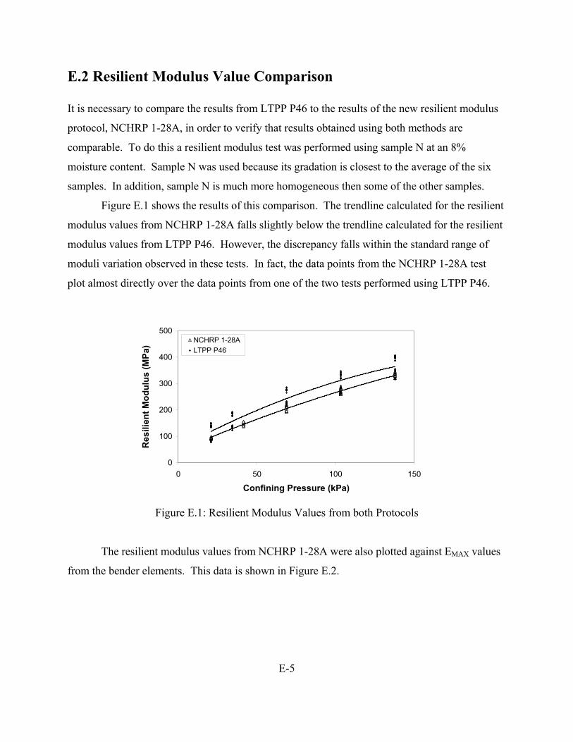
E-5
E.2 Resilient Modulus Value Comparison
It is necessary to compare the results from LTPP P46 to the results of the new resilient modulus
protocol, NCHRP 1-28A, in order to verify that results obtained using both methods are
comparable. To do this a resilient modulus test was performed using sample N at an 8%
moisture content. Sample N was used because its gradation is closest to the average of the six
samples. In addition, sample N is much more homogeneous then some of the other samples.
Figure E.1 shows the results of this comparison. The trendline calculated for the resilient
modulus values from NCHRP 1-28A falls slightly below the trendline calculated for the resilient
modulus values from LTPP P46. However, the discrepancy falls within the standard range of
moduli variation observed in these tests. In fact, the data points from the NCHRP 1-28A test
plot almost directly over the data points from one of the two tests performed using LTPP P46.
Figure E.1: Resilient Modulus Values from both Protocols
The resilient modulus values from NCHRP 1-28A were also plotted against EMAX values
from the bender elements. This data is shown in Figure E.2.
0
100
200
300
400
500
0 50 100 150
Confining Pressure (kPa)
Res
ilien
t Mod
ulus
(MPa
) NCHRP 1-28ALTPP P46
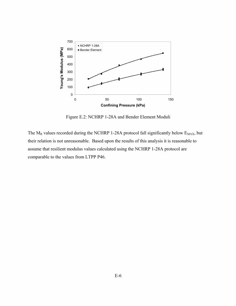
E-6
Figure E.2: NCHRP 1-28A and Bender Element Moduli
The MR values recorded during the NCHRP 1-28A protocol fall significantly below EMAX, but
their relation is not unreasonable. Based upon the results of this analysis it is reasonable to
assume that resilient modulus values calculated using the NCHRP 1-28A protocol are
comparable to the values from LTPP P46.
0
100
200
300
400
500
600
700
0 50 100 150
Confining Pressure (kPa)
Youn
g's
Mod
ulus
(MPa
) NCHRP 1-28ABender Element