Embed Size (px)
Citation preview

Journal of Rehabilitation in Civil Engineering 5-2 (2017) 01-15
journal homepage: http://civiljournal.semnan.ac.ir/
Modeling of Resilient Modulus of Asphalt Concrete
Containing Reclaimed Asphalt Pavement using Feed-
Forward and Generalized Regression Neural
Networks
Ahmad Mansourian1*
, Ali Reza Ghanizadeh2, Babak Golchin
3
1. Department of Bitumen and Asphalt, Road, Housing and Urban Development Research Center, Tehran, Iran
2. Department of Civil Engineering, Sirjan University of Technology, Sirjan, Iran
3. Department of Civil Engineering, Ahar Branch, Islamic Azad University, Ahar, Iran
Corresponding author: [email protected]
ARTICLE INFO
ABSTRACT
Article history:
Received: 16 March 2017
Accepted: 05 September 2017
Reclaimed asphalt pavement (RAP) is one of the waste
materials that highway agencies promote to use in new
construction or rehabilitation of highways pavement. Since
the use of RAP can affect the resilient modulus and other
structural properties of flexible pavement layers, this paper
aims to employ two different artificial neural network (ANN)
models for modeling and evaluating the effects of different
percentages of RAP on resilient modulus of hot-mix asphalt
(HMA). To this end, 216 resilient modulus tests were
conducted for establishing the experimental dataset. Input
variables for predicting resilient modulus were temperature,
penetration grade of asphalt binder, loading frequency,
change of asphalt binder content compared to optimum
asphalt binder content and percentage of RAP. Results of
modeling using feed-forward neural network (FFNN) and
generalized regression neural network (GRNN) model were
compared with the measured resilient modulus using two
statistical indicators. Results showed that for FFNN model,
the coefficient of determination between observed and
predicted values of resilient modulus for training and testing
sets were 0.993 and 0.981, respectively. These two values
were 0.999 and 0.967 in case of GRNN. So, according to
comparison of R2 for testing set, the accuracy of FFNN
method was superior to GRNN method. Tests results and
artificial neural network analysis showed that the
temperature was the most effective parameter on the resilient
modulus of HMA containing RAP materials. In addition by
increasing RAP content, the resilient modulus of HMA
increased.
Keywords:
Asphalt Pavement,
Reclaimed Asphalt,
Resilient Modulus,
Neural Networks.

2 A. Mansourian et al./ Journal of Rehabilitation in Civil Engineering 5-2 (2017) 01-15
1. Introduction Each year millions of tons of asphalt concrete
are produced from damaged asphalt
pavements in the world [1]. The disposal of
this waste material in landfills has been a
traditional solution, but the shortage of
landfill areas, environmental regulations and
related costs have prevented the safe disposal
of these waste products. Investigations show
that using RAP will result in technical,
economical, and environmental benefits [1].
Recently, highway departments promote the
use of RAP in asphalt pavement
rehabilitations. The use of RAP has effect on
some basic properties of hot-mix asphalt
(HMA) such as resilient modulus. Resilient
modulus as a measure of the stiffness of
asphalt concrete mixture is one of the
fundamental parameters that is used in
evaluating of materials quality and as an
input for asphalt pavement design. Colbert
and You [2] evaluated the hot-mix asphalt
containing 15, 35, and 50% RAP
experimentally and indicated that the
addition of RAP increased the resilient
modulus by 52%. Sondag et al. [3] blended 0
to 50% RAP with virgin aggregates and
based on resilient modulus and complex
modulus tests results, recommended different
percentages of RAP (10-50%) and the
respective asphalt binder grades to yield the
stiffness similar to a virgin mixture.
Zaumanis and Mallick [4] investigated the
approaches for increasing the amount of RAP
in asphalt concrete mixtures above 40% and
indicated that the stiffness of high content
RAP asphalt concrete mixtures was higher
than that of the virgin. However the increase
in stiffness was not proportional to RAP
content for all cases.
Nowadays, some asphalt laboratories
generate a lot of resilient modulus data from
their different asphalt concrete mixture tests.
These data are saved in these laboratories
databases. Since, artificial neural network
(ANN) is a computational approach to solve
new problems by applying the information
gained from the past experiences, it seems
that it is possible to use the previous resilient
modulus test data for prediction of resilient
modulus of asphalt concrete mixtures under
other conditions (e.g. temperature, loading
frequency, mix design, and …).
ANN technique has been widely applied in
asphalt material studies. Tarefder et al. [5]
used a four-layer feed-forward neural
network to determine a mapping associating
mix design and testing factors of asphalt
concrete samples to predict their
permeability. They observed an excellent
agreement between simulation and laboratory
data. Ozgan [6] applied an ANN based model
for the results of Marshall stability tests. He
concluded that experiment results and ANN
model exhibit a good correlation. Xiao and
Amirkhanian [7] used ANN approach for
estimating stiffness behavior of rubberized
asphalt concrete containing reclaimed asphalt
pavement. Their results indicated that ANN
techniques were more effective than
traditional regression-based prediction
models in predicting the fatigue life of the
modified mixture. Zaghal [8] modeled creep
compliance behavior of asphalt concretes
using ANN technique. Results of ANN
simulations showed the proposed model
could effectively predict the creep
compliance of asphalt concrete mixtures at
different temperatures with different binders.
ANN has been also used for prediction of
resilient modules of asphalt concrete
mixtures. They are shown in Table 1. Figure
1 shows the research framework.
This research focuses on the prediction of the
resilient modulus of asphalt concrete

A. Mansourian et al./ Journal of Rehabilitation in Civil Engineering 5-2 (2017) 01-15 3
mixtures containing different percentage of
RAP. Two different ANN techniques
including generalized regression neural
network (GRNN) and feed-forward neural
network (FFNN) were applied for prediction
of resilient modulus and their accuracies
have been compared to each other. The
proposed model based on artificial neural
networks helps designers and technicians to
estimate the resilient modulus of asphalt
concretes containing RAP materials with an
appropriate accuracy.
Table 1. Application of ANN in prediction of resilient modulus
Material Inputs Method Main results References
Emulsified
asphalt
mixtures
Curing time
Cement content
Residual content
Back propagation
NN
NN predicts the resilient
modulus with high accuracy. [9]
Rubberized
mixtures
containing
RAP
Rubber content
RAP content
Binder rheology
ANN and regression
models
ANN-based models are more
effective than the regression
models.
[10]
Fiber-
reinforced
asphalt
concrete
Fiber content
Fiber length
Fiber type
Hybrid ANN-
genetic algorithm
model
The optimized ANN can
predict the resilient modulus
with high accuracy.
[11]
Asphalt treated
permeable base
Asphalt contents
Aggregate gradations
Support vector
machines and ANN
SVM model can gain higher
precision than ANN approach. [12]
Figure 1. Research framework

4 A. Mansourian et al./ Journal of Rehabilitation in Civil Engineering 5-2 (2017) 01-15
2. Materials and Test Methods
2.1. Aggregate
The aggregate used in this research study
obtained from an asphalt plant located in the
west part of Tehran. The nominal maximum
aggregate size was 19 mm. Tables 2 and 3
show the aggregate properties and aggregate
gradation, respectively.
Table 2. Aggregate properties
Test Test method Result
Specific gravity ASTM
C-127 2.485
Los Angeles abrasion (%) AASHTO T-96 16
Water absorption (Coarse aggregate) (%) AASHTO T-85 2.6
Water absorption (Fine aggregate) (%) AASHTO T-84 2.5
Percent fracture (one face) (%) ASTM D5821 93
Percent fracture (two faces) (%) ASTM D5821 81
Elongation index BS 812 15
Flakiness index BS 812 25
Table 3. Aggregate gradation
Sieve size (mm) Percent passing
25 100
19 92
9.5 70
4.75 50
2.36 36
0.3 11
0.075 5
2.2. Asphalt binders
The asphalt binders used in this study were
of penetration 60/70 and 85/100 (Pen 60/70
and Pen 85/100). The properties of the
asphalt binders used in this research are
presented in Table 4.
Table 4. Properties of asphalt binders
Test Test method result
60/70 85/100
Specific gravity (25° C) ASTM D70 1.016 1.000
Flash point (Cleveland)(oC) ASTM D92 310 298
Penetration (25° C)(0.1 mm) ASTM D5 69 85
Ductility (25° C) (cm) ASTM D113 >100 >100
Softening point (oC) ASTM D36 49 48
Kinematic viscosity @ 120 ° C (Centistokes) ASTM D2170 832 797
Kinematic viscosity @ 135 ° C (Centistokes) ASTM D2170 440 372
Kinematic viscosity @ 150 ° C C(entistokes) ASTM D2170 137 133

A. Mansourian et al./ Journal of Rehabilitation in Civil Engineering 5-2 (2017) 01-15 5
2.3. Reclaimed asphalt
Reclaimed asphalt in this research was
prepared from an asphalt pavement in
Tehran. Tables 5, 6 and 7 show the properties
of aggregate, aggregate gradation and asphalt
binder extracted from reclaimed asphalt,
respectively.
Table 5. Properties of reclaimed asphalt aggregate
Test Test Method Result
Asphalt binder content (%) ASTM D2172 5.4
Water absorption (Coarse aggregate) (%) ASTM C127 2.1
Water absorption (Fine aggregate) (%) ASTM C128 2.51
Specific gravity (Coarse aggregate) ASTM C127 2.495
Specific gravity (Fine aggregate) ASTM C128 2.502
Table 6. Aggregate gradation of reclaimed asphalt
Sieve size (mm) Percent passing
19 100
9.5 98
4.75 78
2.36 52
0.3 17
0.075 9
Table 7. Properties of extracted asphalt binder
Test Test method result
Penetration (25° C)(0.1 mm) ASTM D5 20
Softening point (oC) ASTM D36 72
Kinematic viscosity @ 135 ° C (Centistokes) ASTM D2170 1977
2.4. Mix design and fabrication of
specimens
The optimum asphalt binder contents of the
control mixtures were determined using
Marshall mix design method (ASTM D1559)
with 75 blows on each side. The optimum
asphalt binder contents were obtained 5.5%
and 4.9% for asphalt containing asphalt
binders of Pen 60/70 and Pen 85/100,
respectively. The asphalt concrete mixtures
containing different percentages of RAP (25,
50 and 75 wt.% of the total mix) were made
by the same optimum asphalt binder content,
so that the amount of asphalt binder would
not confound the analysis of the test results.
2.5 Resilient Modulus Test
When a material is subjected to a stress, the
induced strain will depend on the properties
of the material. In general, the total strain
may be divided to recoverable and non-
recoverable strains. The recoverable part of
strain is called resilient strain and the non-
recoverable is called plastic strain. The
Resilient Modulus (MR) is defined as the
ratio of applied deviator stress to the
recoverable strain (Eq.1) [13].

6 A. Mansourian et al./ Journal of Rehabilitation in Civil Engineering 5-2 (2017) 01-15
dR
r
σM =
ε (1)
Where rε is resilient or recoverable strain and
dσ is the deviator stress.
There are several methods for determining
the resilient modulus of asphalt concrete
mixtures. In this research study the resilient
modulus test was conducted in the indirect
tensile mode and in accordance with ASTM
D4123 [14]. Figure 2 shows the machine
used for determining the resilient modulus of
the asphalt concrete mixtures. The loading
waveform was haversine. In addition the
loading frequencies were 0.33, 0.5 and 1 Hz.
The test was conducted at 5, 25 and 40oC and
then resilient modulus was computed using
the Eq. 2. The specimens remained in the
controlled-temperature chamber at each
temperature for about 24 h prior to testing.
Each specimen was precondition by applying
100 repeated haversine waveform load to
obtain uniform deformation readout. In
according to ASTM D4123 a minimum of 50
to 200 load repetitions is typical. The
magnitudes of loads were 1000 N for tests at
5oC and 500 N for tests at 25
oC and 40
oC. In
accordance with ASTM D4123 the load
range should be that to induce 10 to 50% of
the tensile strength.
R
P(ν 0.27)M
tΔH
(2)
Where MR is resilient modulus (MPa), P is
the magnitude of the dynamic load (N), v is
Poisson ratio, ΔH is the total recoverable
horizontal deformation (mm) and t is the
specimen thickness (mm). The height
(thickness) and diameter of the specimens
were about 70 mm and 102 mm, respectively.
The Poisson ratio (v) may be computed from
Eq. 3 [15].
(3.1849-0.04233t)
0.35ν=0.15+
1+e (3)
Where e is the base of the natural logarithm
(2.7183) and t is the test temperature and is
expressed in degrees Fahrenheit.
Figure 2. Machine for measuring the resilient modulus of asphalt concrete mixtures
Loading Strip
Load Cell
Frame
Specimen
Loading Piston
Frame for Setting
the Sample
Position
LVDT for Measuring
the Horizontal
Displacement System for
Measuring the
Temperature of Skin
and Inside Specimen

A. Mansourian et al./ Journal of Rehabilitation in Civil Engineering 5-2 (2017) 01-15 7
3. Establishment of dataset
The final dataset was established based on
the results of 214 experimental resilient
modulus tests. Input variables (or predictors)
were considered as temperature (5, 25, and
40 oC), penetration grade of asphalt binder
(60/70 and 85/100), loading frequency (0.33,
0.5, and 1 Hz), change of asphalt binder
content compared to the optimum asphalt
binder content (-1, 0, and 1%), and
percentage of RAP (0, 25, 50, and 75%).
Output (or dependent variable) was assumed
as resilient modulus of asphalt concrete
mixtures in MPa. Statistical properties of
different fields of experimental dataset are
given in Table 8.
Table 8. Statistical properties of different fields of dataset.
Statistical Parameter Temperature
(oC)
PGCa
Frequency
(Hz)
CBCb
(%)
RAP
(%)
MR
(MPa)
Minimum 5 0 0.33 -1 0 539
Maximum 40 1 1 1 75 20883
Mean 23.18 0.50 0.61 0.00 37.85 7836.71
Standard Deviation 14.35 0.50 0.29 0.82 27.91 6074.23 aPGC: Penetration grade code (0 for 60/70 asphalt binder and 1 for 85/100 asphalt binder)
bCBC: change of asphalt binder content compared to optimum asphalt binder content
CBC: change of asphalt binder content compared to optimum asphalt binder content
4. Modeling using Artificial Neural
Network (ANN)
The mathematical theory of neural networks
states that every continuous function that
maps intervals of real numbers to some
output interval of real numbers can be
approximated arbitrarily closely by a feed-
forward neural networks with just one hidden
layer [16]. Therefore, in this study artificial
neural network models were developed for
predicting resilient modulus of asphalt
concrete mixtures containing RAP with
respect to different mix parameters, loading
time and temperature.
In order to modeling resilient modulus, two
famous architectures including feed-forward
neural networks (FFNN) and generalized
regression neural networks (GRNN) were
employed. These two architectures of neural
network will be described in the next
sections.
FFNN which is known also as multilayer
perceptron (MLP) is the simplest type of
artificial neural network architecture. In this
network, the information only moves in one
direction from the input layer through the
hidden layers and to the output layer [17].
Analogous to the human brain, a FFNN uses
many simple computational elements, named
artificial neurons, connected by variable
weights [18]. A typical artificial neuron is
illustrated in Figure 3. A FFNN can be
trained to predict a particular function by
adjusting the values of the connections
(weights) between the elements. Neural
networks are trained so that a particular input
leads to a specific target output. The network
is adjusted based on a comparison of the
output and the target until the network output
matches the target. Typically many such
input/target output pairs are used to train a
network.

8 A. Mansourian et al./ Journal of Rehabilitation in Civil Engineering 5-2 (2017) 01-15
Figure 3. Summation and transfer functions of a typical artificial neuron[25].
4.1. Feed-Forward Neural Network
(FFNN)
The training of a FFNN using the back
propagation algorithm involves two phases
[19,20]:
Forward Phase. During this phase, the free
parameters of the network are fixed, and the
input signal is propagated through the
network from input layer to hidden layer and
then to output layer. The forward phase ends
with the computation of an error signal.
iii yde (4)
where di is the desired response, and yi is the
predicted output by the network in response
to the input xi.
Backward Phase. In this phase, the error
signal e is propagated through the network in
the backward direction. In fact in this phase,
adjustments are applied to the free
parameters of the network so as to minimize
the error e in a statistical sense.
In this research, the back propagation
training algorithm of Levenberg - Marquardt
was employed. The architecture of a feed-
forward back propagation neural network has
been presented in Figure 4.
Figure 4. A three layer feed-forward backpropagation network architecture [21].

A. Mansourian et al./ Journal of Rehabilitation in Civil Engineering 5-2 (2017) 01-15 9
4.2. General Regression Neural Network
(GRNN)
Generalized Regression Neural Network
(GRNN) was proposed by Specht [22].
GRNN is a type of ANN which uses a brain
synapse-like structure to handle the
information. The GRNN has good
approximation ability and learning speed
especially for large sample data. The GRNN
also has good forecasting result in case of
small datasets [23].
The main aim of the GRNN is to estimate the
output vector Y=[y1,y2,…,yk]T based on the
input vector X=[x1, x2,…,xn]T by a non-linear
or linear regression surface. The procedure of
the GRNN model can be expressed as
dXXYf
dXXYYf
XYE
),(
),(
]|[
(5)
where X is the input vector with a dimension
of n, Y is the predicted value by GRNN
model, E[Y|X] is the expected value of the
output Y, given the input vector X and f(Y,X)
is the joint probability density function of X
and Y.
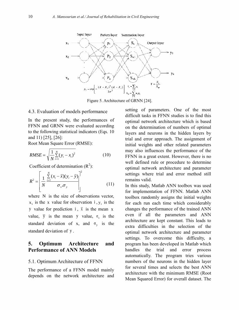
The GRNN is organized using four layers
including input layer, pattern layer,
summation layer, and output layer (Figure 5).
The input layer receives input parameters and
stores them to an input vector X. Number of
neurons in input layer is equal to the
dimension of input vector. Then, the data
from input layer are fed to the pattern layer.
The pattern layer implements a non-linear
transformation from the input space to the
pattern space. The neurons in the pattern
layer can memorize the relationship between
the input neuron and the proper response of
pattern layer. The number of neurons in
hidden layer is equal to the number of input
variables. The pattern Gaussian function of pi
is as follows: T
i ii 2
(X-X ) (X-X )p =exp - (i=1,2,...,n)
2σ
(6)
Where σ is the smoothing parameter, X is the
input variable and Xi is a specific training
vector of the neuron i in the pattern layer.
The summation layer has two summations
which are Ss and Sw. The simple summation
Ss computes the arithmetic sum of the pattern
layer outputs, and the interconnection weight
is equal to ‘1’. The weighted summation Sw
computes the weighted sum of the pattern
layer outputs, and the interconnection weight
is w. These two parameters can be
represented as Eqs. (7) and (8), respectively:
s ii=1
S = p (7)
w i ii=1
S = w p (8)
Where wi is the weight of pattern neuron i
connected to the summation layer.
The number of neurons in the output layer is
equal to the dimension k of the output vector
Y. After commutating the summations of
neurons in the summation layer, they are fed
into the output layer. The output Y of the
GRNN model can be determined as follows:
s
w
SY=
S (9)
As can be seen, the GRNN model has only
one parameter σ that needs to be determined.
The parameter σ determines the
generalization capability of the GRNN.
10 A. Mansourian et al./ Journal of Rehabilitation in Civil Engineering 5-2 (2017) 01-15
Figure 5. Architecture of GRNN [24].
4.3. Evaluation of models performance
In the present study, the performances of
FFNN and GRNN were evaluated according
to the following statistical indicators (Eqs. 10
and 11) [25], [26]:
Root Mean Square Error (RMSE):
(10)
Coefficient of determination (R2):
(11)
where N is the size of observations vector,
ix is the x value for observation i , iy is the
y value for prediction i , x is the mean x
value, y is the mean y value, xσ is the
standard deviation of x, and yσ is the
standard deviation of y .
5. Optimum Architecture and
Performance of ANN Models
5.1. Optimum Architecture of FFNN
The performance of a FFNN model mainly
depends on the network architecture and
setting of parameters. One of the most
difficult tasks in FFNN studies is to find this
optimal network architecture which is based
on the determination of numbers of optimal
layers and neurons in the hidden layers by
trial and error approach. The assignment of
initial weights and other related parameters
may also influences the performance of the
FFNN in a great extent. However, there is no
well defined rule or procedure to determine
optimal network architecture and parameter
settings where trial and error method still
remains valid.
In this study, Matlab ANN toolbox was used
for implementation of FFNN. Matlab ANN
toolbox randomly assigns the initial weights
for each run each time which considerably
changes the performance of the trained ANN
even if all the parameters and ANN
architecture are kept constant. This leads to
extra difficulties in the selection of the
optimal network architecture and parameter
settings. To overcome this difficulty, a
program has been developed in Matlab which
handles the trial and error process
automatically. The program tries various
numbers of the neurons in the hidden layer
for several times and selects the best ANN
architecture with the minimum RMSE (Root
Mean Squared Error) for overall dataset. The
2
1
) (1
i
N
ii xy
NRMSE
2
12
.
))((1
yx
N
iii yyxx
NR
A. Mansourian et al./ Journal of Rehabilitation in Civil Engineering 5-2 (2017) 01-15 11
testing (20%), cross validating (10%) and
training (70%) sets for ANN training
procedure were selected randomly from the
established database. The optimal ANN
architecture was found to be 5-14-1 (one
hidden layer with 20 neurons). Hyperbolic
tangent sigmoid and linear transfer functions
were used for the hidden layers and output
layer, respectively. More details are presented
in appendix A.
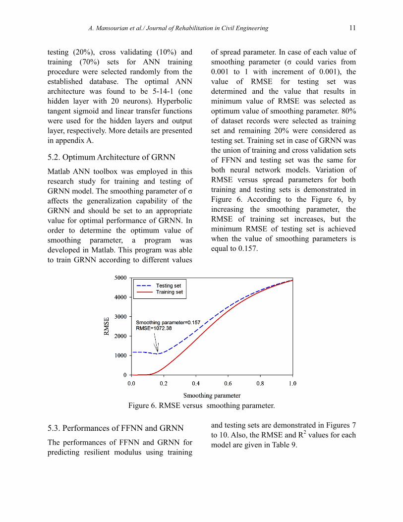
5.2. Optimum Architecture of GRNN
Matlab ANN toolbox was employed in this
research study for training and testing of
GRNN model. The smoothing parameter of σ
affects the generalization capability of the
GRNN and should be set to an appropriate
value for optimal performance of GRNN. In
order to determine the optimum value of
smoothing parameter, a program was
developed in Matlab. This program was able
to train GRNN according to different values
of spread parameter. In case of each value of
smoothing parameter (σ could varies from
0.001 to 1 with increment of 0.001), the
value of RMSE for testing set was
determined and the value that results in
minimum value of RMSE was selected as
optimum value of smoothing parameter. 80%
of dataset records were selected as training
set and remaining 20% were considered as
testing set. Training set in case of GRNN was
the union of training and cross validation sets
of FFNN and testing set was the same for
both neural network models. Variation of
RMSE versus spread parameters for both
training and testing sets is demonstrated in
Figure 6. According to the Figure 6, by
increasing the smoothing parameter, the
RMSE of training set increases, but the
minimum RMSE of testing set is achieved
when the value of smoothing parameters is
equal to 0.157.
Figure 6. RMSE versus smoothing parameter.
5.3. Performances of FFNN and GRNN
The performances of FFNN and GRNN for
predicting resilient modulus using training
and testing sets are demonstrated in Figures 7
to 10. Also, the RMSE and R2 values for each
model are given in Table 9.

12 A. Mansourian et al./ Journal of Rehabilitation in Civil Engineering 5-2 (2017) 01-15
Figure 7. Performance of FFNN model (training set).
Figure 8. Performance of FFNN model (testing set).
Figure 9. Performance of GRNN model (training set).
A. Mansourian et al./ Journal of Rehabilitation in Civil Engineering 5-2 (2017) 01-15 13
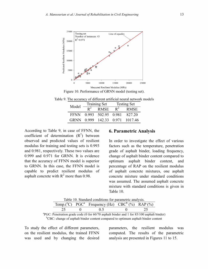
Figure 10. Performance of GRNN model (testing set).
Table 9. The accuracy of different artificial neural network models
Model Training Set Testing Set
R2 RMSE R
2 RMSE
FFNN 0.993 502.95 0.981 827.20
GRNN 0.999 142.33 0.971 1017.46
According to Table 9, in case of FFNN, the
coefficient of determination (R2) between
observed and predicted values of resilient
modulus for training and testing sets is 0.993
and 0.981, respectively. These two values are
0.999 and 0.971 for GRNN. It is evidence
that the accuracy of FFNN model is superior
to GRNN. In this case, the FFNN model is
capable to predict resilient modulus of
asphalt concrete with R2 more than 0.98.
6. Parametric Analysis
In order to investigate the effect of various
factors such as the temperature, penetration
grade of asphalt binder, loading frequency,
change of asphalt binder content compared to
optimum asphalt binder content, and
percentage of RAP on the resilient modulus
of asphalt concrete mixtures, one asphalt
concrete mixture under standard conditions
was assumed. The assumed asphalt concrete
mixture with standard conditions is given in
Table 10.
Table 10. Standard conditions for parametric analysis.
Temp.(oC) PGC
a Frequency (Hz) CBC
b (%) RAP (%)
25 0 0.5 0 25 aPGC: Penetration grade code (0 for 60/70 asphalt binder and 1 for 85/100 asphalt binder)
bCBC: change of asphalt binder content compared to optimum asphalt binder content
To study the effect of different parameters,
on the resilient modulus, the trained FFNN
was used and by changing the desired
parameters, the resilient modulus was
computed. The results of the parametric
analysis are presented in Figures 11 to 15.

14 A. Mansourian et al./ Journal of Rehabilitation in Civil Engineering 5-2 (2017) 01-15
Figure 11. Effect of temperature on the resilient modulus of asphalt concrete mixture.
Figure 12. Effect of penetration grade of asphalt binder on the resilient modulus of asphalt concrete
mixture.
Figure 13. Effect of loading frequency on the resilient modulus of asphalt mixure.

A. Mansourian et al./ Journal of Rehabilitation in Civil Engineering 5-2 (2017) 01-15 15
Figure 14. Effect of CBC parameter on the resilient modulus of asphalt mixure.
Figure 15. Effect of RAP content on the resilient modulus of asphalt concrete mixture
According to Figures 11 to 15, the effect of
different parameters on the resilient modulus
of asphalt concrete mixtures can be stated as
follows:
Temperature: by increasing the temperature,
the resilient modulus of asphalt mixes
decreases and vice versa. Due to visoelastic
behavior of asphalt materials, by increasing
temperature, the viscosity of asphalt binder
decreases and thus the stiffness of asphalt
concrete decreases.
Change of asphalt binder content compared
to optimum asphalt binder content: by
increasing asphalt binder content compared
to optimum asphalt binder content, resilient
modulus increases. Also by decreasing
asphalt binder content compared to optimum
asphalt binder content, resilient modulus
decreases. As the asphalt binder content
increases, the adhesion and tensile strength in
the mixture structure improves. This leads to
decrease in the horizontal deformation in the
resilient modulus test, so in according to
equation 2, the resilient modulus of asphalt
concrete mixtures increases. However it
should be noted that if the asphalt binder

16 A. Mansourian et al./ Journal of Rehabilitation in Civil Engineering 5-2 (2017) 01-15
content increases so much, the excess asphalt
binder will weak the interlocking the
aggregate and so the resilient modulus of
asphalt concrete mixture will decrease.
Penetration grade of asphalt binder: by
increasing the Penetration grade, the resilient
modulus of asphalt mixes decreases and vice
versa. Asphalt binder with higher penetration
grade has lower viscosity and this decreases
the stiffness and resilient modulus of the
asphalt concrete mixtures.
Loading frequency: by changing loading
frequency between 0.5 to 0.9 Hz, no
distinctive change is observed for resilient
modulus. This can be explained by narrow
range of frequency change.
In fact for exploring the effect of frequency
on the resilient modulus of asphalt concrete,
the frequency should be changed in a wide
range specially for moderate and low
temperatures.For further research, it is
recommended that a wide range of
frequencies (from 0.1 to 10) to be used for
experimental program.
RAP content: By Increasing RAP content, the
resilient modulus of asphalt mixes increases,
significantly. Since, RAP contains aged
asphalt binder, so the addition of RAP makes
the mixture stiffer and increases the resilient
modulus. It should be noted that although the
increasing of resilient modulus may
considered as a positive parameter for
pavement design, but the other properties
such as fatigue and rutting resistance of
asphalt concrete mixture containing RAP
should be evaluated.
7. Conclusion
In this study, two different versions of
artificial neural networks including FFNN
and GRNN, were employed for modeling of
the resilient modulus of asphalt concrete
mixtures containing reclaimed asphalt
pavement. In ANN architecture, temperature
(oC), penetration grade code (0 for 60/70
asphalt binder and 1 for 85/100 asphalt
binder), loading frequency (Hz), change of
asphalt binder content compared to optimum
asphalt binder content (%), and RAP content
(%) were chosen as the input parameters and
the resilient modulus (MPa) of asphalt
concrete mixtures was assumed as the output
parameter.
According to the results of this study the
following statements can be concluded:
- The optimum architecture of FFNN for
predicting resilient modulus was determined
as 5-14-1 (one hidden layer) with hyperbolic
tangent sigmoid and linear transfer functions
for the hidden layer and output layer,
respectively. R2 and RMSE for predicted
values of resilient modulus using FFNN was
determined as 0.981 and 827.20 for testing
set, while these values are 0.971 and 1017.46
in case of GRNN. Thus, the accuracy of
FFNN model was superior to GRNN model
for predicting resilient modulus of asphalt
concrete mixtures containing RAP materials.
- The most effective parameter on the
resilient modulus of asphalt concrete
mixtures containing RAP materials was
temperature.
- The resilient modulus of asphalt concrete
mixtures increased when the RAP content
increases or stiffer asphalt binder is
employed.
- Results of this study also showed that by
decreasing temperature and increasing
asphalt binder content compared to optimum
asphalt binder content, resilient modulus
increases.

A. Mansourian et al./ Journal of Rehabilitation in Civil Engineering 5-2 (2017) 01-15 17
References
1. West, R.C., Rada, G.R., Willis, J.R.,
Marasteanu, M.O. (2013), NCHRP report
752, Improved Mix Design, Evaluation and
Materials Management Practices for Hot Mix
Asphalt with High Reclaimed Asphalt
Pavement Content, TRB, National Research
Council, Washington, DC, USA.
2. Colbert, B., You, Z. (2012). The
Determination of Mechanical Performance of
Laboratory Produced Hot Mix Asphalt
Mixtures Using Controlled RAP and Virgin
Aggregate Size Fractions, Construction and
Building Materials, 26:655-662. (DOI:
10.1016/j.conbuildmat.2011.06.068)
3. Sondag, M.S., Chadbourn, B.A., Drescher,
A. (2002). Investigation of Recycled Asphalt
Pavement (RAP) Mixtures, Minnesota
Department of Transportation, Report No:
MN/RC - 2002-15.
4. Zaumanis, M., Mallick, R.B. (2015).
Review of Very High-Content Reclaimed
Asphalt Use in Plant-Produced Pavements:
State of the Art, International Journal of
Pavement Engineering, 16: 39-55. (DOI:
10.1080/10298436.2014.893331)
5. Tarefder, R.A., White, L., Zaman, M.
(2005). Neural Network Model for Asphalt
Concrete Permeability, Journal of Materials
in Civil Engineering, 17:19-27. (DOI:
10.1061/(ASCE)0899-1561(2005)17:1(19))
6. Ozgan, E. (2011). Artificial Neural
Network Based Modeling of the Marshall
Stability of Asphalt Concrete, Expert
Systems with Applications, 38:6025-6030.
(DOI: 10.1016/j.eswa.2010.11.018)
7. Xiao, F., Amirkhanian, S.N. (2009).
Artificial Neural Network Approach to
Estimating Stiffness Behavior of Rubberized
Asphalt Concrete Containing Reclaimed
Asphalt Pavement, Journal of Transportation
Engineering, 135:580-589. (DOI:
10.1061/(ASCE)TE.1943-5436.0000014)
8. Zeghal, M. (2008). Modeling the Creep
Compliance of Asphalt Concrete Using the
Artificial Neural Network Technique,
GeoCongress: Characterization, Monitoring
and Modeling of GeoSystems, 910-916.
(DOI: 10.1061/40972(311)114)
9. Ozsahin, T.S., Oruc, S. (2008). Neural
Network Model for Resilient Modulus of
Emulsified Asphalt Mixtures, Construction
and Building Materials, 22:1436-1445.
(DOI:10.1016/j.conbuildmat.2007.01.031)
10. Xiao, F., Amirkhanian, S.N. (2008).
Effects of Binders on Resilient Modulus of
Rubberized Mixtures Containing RAP Using
Artificial Neural Network Approach, Journal
of Testing and Evaluation, 37:129-138. (DOI:
10.1520/JTE101834)
11. Vadood, M., Johari, M.S., and Rahai, A.
(2015). Developing a Hybrid Artificial
Neural Network-Genetic Algorithm Model to
Predict Resilient Modulus of
Polypropylene/Polyester Fiber-Reinforced
Asphalt Concrete, The Journal of the Textile
Institute, 106:1239-1250. (DOI:
10.1080/00405000.2014.985882)
12. Kezhen, Y., Yin, H., Liao, H., Huang, L.
(2011) Prediction of Resilient Modulus of
Asphalt Pavement Material Using Support
Vector Machine, Road pavement and
material characterization, modeling, and
maintenance, 16-23. (DOI:
10.1061/47624(403)3)
13. Huang, Y.H. (2004), Pavement Design
and Analysis. Pearson/Prentice Hall.
14. ASTM D4123, Standard Test Method for
Indirect Tension Test for Resilient Modulus
of Bituminous Mixtures. (1995) West
Conshohocken, PA: ASTM International,
USA.
15. Witzcak, M.W., Kaloush, K., Pellinen, T.,
El-Basyouny, M, Von Quintus, H. (2002).

18 A. Mansourian et al./ Journal of Rehabilitation in Civil Engineering 5-2 (2017) 01-15
Simple Performance Test for Superpave Mix
Design (Vol. 465), TRB, National Research
Council, Washington, DC, USA.
16. Hornik, K. (1991). Approximation
Capabilities of Multilayer Feed-forward
Networks, Neural Networks, 4:251–257.
(DOI: 10.1016/0893-6080(91)90009-T)
17. Hagan, M.T., Demuth, H.B., Beale M.H.
(1996), Neural Network Design, PWS Pub.
Co., Boston, USA.
18. Haykin, S.S. (2001), Neural Networks: a
Comprehensive Foundation, Tsinghua
University Press.
19. Werbos, P. (1974), Beyond regression:
New Tools for Prediction and Analysis in the
Behavioral Sciences.
20. Rumelhart, D.E., Hinton G.E., Williams,
R.J. (1988). Learning Representations by
back-Propagating Errors, Cognitive
Modeling 5:1.
21. Freeman, J.A., Skapura, D.M., (1992),
Neural Networks: Algorithms, Applications
and Programming Techniques, Addison-
Wesley Publishing Company.
22. Specht, D.F., (1991). A General
Regression Neural Network, IEEE
Transactions on Neural Networks, 2:568-576.
(DOI: 10.1109/72.97934)
23. Li, H.Z., Guo, S., Li, C.J., Sun, J.Q.
(2013). A Hybrid Annual Power Load
Forecasting Model Based on Generalized
Regression Neural Network with Fruit Fly
Optimization Algorithm, Knowledge-Based
Systems, 37:378-387. (DOI:
10.1016/j.knosys.2012.08.015)
24. Leung, M.T., Chen, A.S., Daouk, H.
(2002). Forecasting Exchange Rates Using
General Regression Neural Networks,
Computers & Operations Research, (DOI:
27:1093–1110. 10.1016/S0305-
0548(99)00144-6)
25. Khademi, F., Jamal, S. M., Deshpande,
N., & Londhe, S. (2016). Predicting strength
of recycled aggregate concrete using artificial
neural network, adaptive neuro-fuzzy
inference system and multiple linear
regression. International Journal of
Sustainable Built Environment, 5(2), 355-
369.
26. Khademi, F., Akbari, M., Jamal, S. M., &
Nikoo, M. (2017). Multiple linear regression,
artificial neural network, and fuzzy logic
prediction of 28 days compressive strength of
concrete. Frontiers of Structural and Civil
Engineering, 11(1), 90-99.
Appendix A. Weights and biases of
Artificial Neural Network (ANN)
This Appendix is assigned to input vector,
output vector, weight factors, and bias factors
of the back propagation neural network
which was discussed in section 4.5. The
optimum architecture of back propagation
neural network is 5-14-1 with sigmoid
transfer function in the hidden layer and
linear transfer function in the output layer.
The order of normalized predictors in the
input vector is as follows:
1×5
I= T,PGC,Frequency,CBC,RAP (12)
The order of normalized output parameters in
the output vector is as follows:
1×1
O= Mr (13)
Equation (14) may be used for simulation of
ANN and prediction of resilient modulus
based on given input vector.
T T TT
h h o oOut =tansig Inp × W + θ × W + θ
(14)
Where tansig (x) can be obtained as follows:
-2x
2tansig(x)= -1
1+e (15)
Weight matrix for hidden and output layers
are given in Table 11 and Table 12,
respectively. Bias vector for hidden and

A. Mansourian et al./ Journal of Rehabilitation in Civil Engineering 5-2 (2017) 01-15 19
output layer are given in Table 13 and Table 14, respectively.
Table 11. Weight matrix of hidden layer (Wh)t14×5
-0.299643482 0.331131154 -0.150468515 3.894341144 -1.668650763
1.245192212 -0.474771598 -0.018442791 -2.452333208 3.068082506
1.748791212 0.145061223 -0.767821500 0.608096855 -0.051696506
-1.423850700 0.280712802 -0.191103718 0.395230798 -0.118328016
-1.809273169 0.145292928 1.949744431 0.989839148 -2.461689208
-0.922523725 0.689167058 0.620551910 -1.382514250 1.110017441
2.213075920 1.798941169 1.390372619 0.573364045 -0.215540190
-2.105617879 0.003661187 0.046071359 -0.625417854 0.838355064
-1.101012107 -1.135496135 0.468455867 -7.184626798 -0.977689316
2.425698003 1.168375909 -0.318634537 -1.986476824 -0.819925948
2.054786137 -1.787104430 0.994535680 2.862659074 -2.284213323
0.960594508 -0.912956687 -0.138879608 3.623386289 2.789123777
-0.290257636 1.097970413 0.150710357 -1.003233075 2.653275383
-0.762431346 -1.915528492 1.229452135 1.775558134 1.225965169
Table 12. Weight matrix of output layer (Wo)
14×1
-0.295478876
-0.204809027
0.083193339
0.397573892
0.024329070
0.064349455
-0.060940316
0.289739736
0.077479325
-0.104030104
0.057266017
0.105736230
0.175164928
0.022502847
Bias vector for hidden and output layer are
given in Table 13 and Table 14, respectively:
Table 13. Bias vector of hidden layer (θh)
-4.765303345
3.153745569
-2.332963106
-0.607005988
-1.178814078
1.336729674
1.370637157
0.275829938
-2.188464110
1.655692989
-1.621861283
2.530472150
-4.183043913
-2.608443726
Table 14. Bias vector of output layer (θo)
-0.017525849