Skin Lesion Tracking using Structured Graphical Models

Hengameh Mirzaalian1,2, Tim K Lee1,2,3, and Ghassan Hamarneh1

1Medical Image Analysis Lab, Simon Fraser University, BC, Canada.2Photomedicine Institute, Department of Dermatology and Skin Science, University of British Columbia and Vancouver Coastal Health

Research Institute, BC, Canada.3Cancer Control Research, BC Cancer Agency, BC, Canada.

Abstract

An automatic pigmented skin lesions tracking system, which is important for early skin cancer detection, isproposed in this work. The input to the system is a pair of skin back images of the same subject captured atdifferent times. The output is the correspondence (matching) between the detected lesions and the identi-fication of newly appearing and disappearing ones. First, a set of anatomical landmarks are detected usinga pictorial structure algorithm. The lesions that are located within the polygon defined by the landmarksare identified and their anatomical spatial contexts are encoded by the landmarks. Then, these lesions arematched by labelling an association graph using a tensor based algorithm. A structured support vector ma-chine is employed to learn all free parameters in the aforementioned steps. An adaptive learning approach(on-the-fly vs offline learning) is applied to set the parameters of the matching objective function usingthe estimated error of the detected landmarks. The effectiveness of the different steps in our framework isvalidated on 194 skin back images (97 pairs).

Keywords: Melanoma; Pigmented Skin Lesion; Anatomical Landmark; Feature (lesion and landmark)Detection; Lesion Tracking; Point Matching; Graph Matching; Graphical Models; Structured SupportVector Machines; Hyperparameter Learning; Error Prediction; Uncertainty Encoding.

1. Introduction

1.1. BackgroundMalignant melanoma (MM) is one of the common cancers among the white population [1]. It has been

shown that the presence of a large number of pigmented skin lesions (PSLs) is an important risk factor forMM [2]. For early detection of MM, dermatologists advocate total body photography for high-risk patients.Regular examination and comparison of the skin using 2D digital pictures collected at different timescan help identify newly-appearing, disappearing, and changing PSLs [3]. However, tracking PSLs in skinimages is time consuming and error prone with large inter- and intra-rater variability. Recently, a few workshave been proposed towards an automatic system for tracking PSLs [4, 5, 6], which mostly focused on thePSL matching task, where the positions of the PSLs and a set of anatomical landmarks (LNDs) are assumedto be known. In order to develop an end-to-end PSL tracking system, we need to detect the PSLs and LNDsautomatically as well as perform PSL matching. In the remaining of the introduction section, we reviewthe steps required for building such an automatic PSL tracking system.

Preprint submitted to Journal of Medical Image Analysis March 25, 2015

[Ref] Unary Binary Ternary Optimization approach Learning[4] X × × Dynamic Programming ×

[14, 15] X X × Taylor expansion and Gradient descent ×[16] X X X Taylor expansion and Gradient descent X[17] X X × Dual decomposition ×[18] X X X Dual decomposition ×

[19, 20, 21, 22] X × × Genetic algorithm ×[23] X × × Expectation-maximization ×

[24, 25, 26, 27, 28, 29, 30] X X × Expectation-maximization ×[31] X X × Marginalization ×[32] X X X Marginalization ×

[33, 34, 6] X X × Spectral based ×[35, 36] X X × Spectral based X

[37, 38, 5] X X X Spectral based ×Proposed X X X Spectral based X

Table 1: Comparison between different point matching methods in terms of the order of the energy terms in the cost function (unary,binary, and ternary), the optimization approach, and the hyperparameter learning.

LND Detection. There exist many techniques for automatic LND detection based on feature points [7, 8,9, 10]. In general, these methods consider a set of appearance models of the LNDs and their geometricrelations to regularize the final detected LNDs. To the best of our knowledge, no work has been done onautomatic LND detection on skin-back images.PSL Detection. A notable number of methods have been proposed for PSL segmentation on dermoscopicimages, which show close-ups on lesions, but not for skin back images in total-body photography, whichare two different problems. The following are the key existing works on PSL detection on wide-area skinimages. Sang et al. [11] detected potential PSL candidates on skin images of human arms by using featurevectors of steerable filter responses as input to a support vector machine (SVM) classifier. Pierrard et al.[12] applied Laplacian of Gaussian filter to enhance PSLs and then defined a saliency measurement to selectthe potential enhanced structures on face skin images. The most closely related PSL detection method forour application (i.e. back images) is the one by Lee et al. [13], in which they, first, applied thresholdingto the output of an image enhanced by an adaptive Gaussian kernel. Then, they detected potential PSLcandidates in the thresholded binary image based on geometric feature (e.g. area and elongation).PSL Matching. Finding the mapping between the PSLs in a pair of images can be formulated as a graphmatching problem. There exists extensive research on point matching as a graph labeling problem. Ingeneral, these methods construct a matching cost function including unary, binary, and ternay terms tomeasure matching compatibilities between the single, pair-wise, and triplet-wise correspondences. A com-mon basic constraint is that each vertex in one graph be mapped to at most one point in the other one, andvice versa. To search for a crisp solution or a fuzzy solution different optimization approaches have beenapplied to minimize the matching cost function, e.g. dual decomposition, spectral and tensor based formu-lation, successive projections to find marginalization-matrix, gradient descent on taylor expansion, geneticalgorithm, and expectation-maximization. In Table 1, we compare the state-of-the-art point matching algo-rithms in terms of the order of the cost function (single, pair-wise, and triplet-wise) and the optimizationapproach.

Despite extensive research on graph matching, only a few works specifically focus on PSL matching.Huang and Bergstresser [4] developed a PSL matching algorithm using a PSL-based Voronoi decompositionof the image space. However, the Voronoi decomposition changes dramatically when one or more PSLs

2

appear or disappear causing the matching to fail. To normalize PSL coordinates prior to PSL matching,we previously proposed a landmark-based non-rigid warping of the back images to a unit-square template[5, 6]. However, this approach suffers form the following weaknesses: it requires an accurate segmentationof the back silhouette; the warping is influenced by all landmarks equally, even when certain landmarksare clearly more stable than others; and undesired distortions may occur for subjects requiring large warps.

Another observation on the existing point matching algorithms is that only a few papers propose asolution for learning the optimal set of parameters for graph matching. Leordeanu et al. [35, 16] appliedgradient descent to minimize the error of their non-convex spectral-based formulation. Caetano et al. [36]applied a max-margin structured estimation technique to learn the parameters of quadratic assignmentrelaxation problems.

1.2. Our contributionsWe formulate all the aforementioned steps (LND detection, PSL localization, and PSL matching) as op-

timization problems. Our first contribution is parts-based graphical models [39] for detecting the LNDs.The detected LNDs serve two purposes: They restrict the search space to a polygon during lesion localiza-tion and encode the anatomical spatial context of lesions (Section 2.1). The latter encoding is a novel PSLdescriptor that we leverage for PSL matching.

Our second contribution is to improve PSL-detection approaches by using a new set of Hessian baseddescriptors (Section 2.3). Applying a random forest (RF) classifier, we compute a likelihood map for thepresence of PSLs. Then, only the pixels inside the aforementioned polygon having a large likelihood valueand belonging to a large enough connected component, are used in the subsequent PSL matching (Section2.3).

As Our third contribution, we devise a new landmark based PSL descriptor that encodes uncertaintyin the automatically detected LNDs and does not rely on any warping (Section 2.4). This descriptor isreminiscent of shape context [27], with the key conceptual difference that we capture spatial context withrespect to the anatomical landmarks without constructing any histogram.

Similar to many medical image analysis problems, our formulations require setting objective functionswith hyperparameters. In the fourth contribution, we apply structured support vector machine (SSVM) [40]to learn the free parameters (Sections 2.2). Thus, the proposed system is called a structured skin lesiontracking system.

Because of the dependence of the PSL descriptors on the detected LNDs, in our final contribution, wepropose an adaptive system that, first, predicts the error in the detected LNDs and, then leverages themeasured error to adapt (on-the-fly vs offline learning) the PSL matching (Section 2.6).

In contrast to the earlier works on graph matching (Table 1), our PSL matching technique uses thethree terms (unary, binary, ternary) together using a spectral based optimization algorithm. We learn thehyperparameters of our objective function using SSVM.

In Table 2, we compare existing works on automatic lesion tracking systems. In contrast to the previousworks on skin lesion tracking, the three tasks of LND detection, PSL detection, and PSL matching areperformed automatically. Further, our method is unique in including parameter learning and considerationof uncertainty and predicted-error.

We evaluate the effectiveness of the different steps in our framework on 194 skin back color images (97pairs). The results are presented in Section 3, followed by concluding remarks in Section 4.

3

Method Auto Auto Auto Learning Measuring PredictingLND PSL Matching Params Uncertainty Error

[41, 4, 6, 42, 5] × × X × × ×[13, 12, 11] × X × × × ×[35, 16, 36] × × X X × ×[5] × × X × X ×Proposed X X X X X X

Table 2: Comparison between different methods in terms of automating different steps (LND detection, PSL detection, PSL matching),parameter learning, and consideration of uncertainty and predicted-error.

2. Method

A summary of our framework is presented in Figure 1. Given two 2D color skin images I and I ′ , thegoal is to detect PSLs in these two images and match (correspond) them. Let V represent the set of PSLsin I (similarly for V ′ in I ′). We define a matching matrix X , such that if Vi ∈ V matches (corresponds to)V ′j ∈ V

′ then Xij = 1 (and 0 otherwise). Corresponding PSLs must have homologous positions with respectto anatomical landmarks (LNDs). As in [6], we use the left and right neck, shoulder, armpit, and hip pointsas our landmarks and denote their spatial coordinates by Li , i = 1...8, in I (similarly for L′i in I ′). Thereare three main stages in our algorithm: (i) LND Detection, (ii) PSL Detection, and (iii) PSL Matching.

In short, we formulate all the LND detection, PSL detection and matching objectives as linear combina-tions of different terms as shown in Table 3. In Table 4, we provide a list of frequently used acronyms inthe following sections.

Problem Unknown Objective functionWeights and terms Optimization

(u: unary, b:binary, t: ternary) method

LND detectionL landmarks in image I

E(L) = wTLφL(L,I ) wL =

[wuLwbL

]φL(L) =

[φuL (L)φbL(L)

]Pictorial [39]L′ landmarks in image I ′

PSL detectionP lesion locations in I

E(P ) = wTP φP (P ,I ) wP =

[wuP

]φP (X ) =

[φuP (P )

]Random forest [43]P ′ lesion locations in I ′

PSL matching X matching matrix E(X ) = wTMφM (X ,P ,P ′) wM =

wuMwbMwtM

φM (X ) =

φuM (X )φbM (X )φtM (X )

Tensor based [37]

• {φu ,φb ,φt} correspond to the unary, binary, and ternary terms, respectively.• {φu ,wu } ∈Ru , {φb ,wb} ∈Rb , {φt ,wt} ∈Rt .• {Ru ,Rb ,Rt} dimensions depend on the unary, binary, and ternary descriptors in our formulations.

Table 3: General formuations of the LND detection, PSL detection and matching problems in our framework.

MM Malignanet melanoma PSL Pigmented skin lesionsLND Landmark RF Random forestSVM Support vector machine SSVM Structured SVM

Table 4: Table of acronyms.

4

(a) I , I ′

NrSrAr NrSrAr

(b) φL(I ),φL(I ′)

Nl Nr

Sl Sr

Al Ar

Hl Hr

(c)

(d) L, L′ (e) V , V ′ (f) X

Figure 1: Summary of our framework. (a) Two skin back images of the same subject. (b) Computed likelihoods of the right neck,shoulder, and armpit LNDs encoded into the RGB channels (1). (c) The tree resulting from applying the minimum spanning treealgorithm computed in the training phase, which is used in the pictorial algorithm (Section 2). (d) Detected LNDs (1). (e) Theoverlaid colored line segments connecting the PSL to the landmarks visualize the approach used to compute the landmark contextfeature (14). The vertices of the black polygons are the LNDs in (d). (f) PSL correspondences (13) and two newly appearing PSLs arehighlighted within the red box.

2.1. LND DetectionThe goal here is to find the LNDs L1...L8 ∈ L and L′1...L

′8 ∈ L′ , which we formulate as an optimization

problem (similar optimization approach is applied to detect L′ in I ′):

L(I ) = argminL

wTLφL(L,I ) (1)

wL = [w1L...w

8L wo

L ]T, φL(L,I ) = [φ1L(L1,I ) ... φ8

L(L8,I ) φoL(L)]T

where Li is a 2×1 vector representing 2D spatial coordinate of the ith LND within the image domain, i.e.the search space for the coordinates of the ith LND is the finite set of all image pixel coordinates; wL is avector of scalars encoding weights of the different energy terms in φ; φoL(L) =

∑ij φ

oL(Li ,Lj ) is the sum of

the mahalanobis distance between all landmark pairs:

φo(Li ,Lj ) = (Lij − Lij )TC−1ij (Lij − Lij ) (2)

where Lij and Cij are the mean and covariance matrix of the edges (vectors) Lij = Li −Lj (connecting Li toLj ) in the training dataset:

Lij =

N∑n=1

∗Lkij

N, Cij =

N∑n=1

[∗Lkij − Lij ][

∗Lkij − Lij ]

T

N − 1(3)

5

where∗Lk represents ground truth landmark information of the kth image. This pairwise regularization

term encourages the vector Lij to conform to a learnt graphical model.φiL(Li ,I ) in (1), i = 1...8, are the data (unary) terms that penalize locating the ith LND at Li , each is

captured using: local binary pattern-based features [44] of the RGB and HSV channels (6 features), xyspatial coordinates of the pixels (2 features), and Frangi et al. [45] filtered response (2 scales). Consideringa 5×5 local window, the final feature vector to compute the data terms φiL is of size 250 (=25×[6+2+2]). Weextract the aforementioned features from 200 windows (per image in the training dataset) centered aroundthe position of the landmarks as true positive samples and a set of randomly selected windows not near theposition of the landmarks as true negative samples. These positive and negative samples are used to traina random forest classifier. Examples of the measured φiL, i = 1...3, are shown in Figure 1(b).

We apply the pictorial structures algorithm [39] to globally optimize the final LND detection cost func-tion (1). The algorithm in [39] is a recursive algorithm that requires computing the regularization termover an acyclic graph (tree) connecting the LNDs. To find the tree structure, we compute the minimumspanning tree (MST) over a complete graph with the 8 LNDs as vertices and with edge weights set as thecovariance values of the edges [39]. Example of the computed MST tree is shown in Figure 1(c).

2.2. Structured Hyperparameter LearningThe LND optimization in (1) requires the knowledge of wL. We apply SSVM [40] to estimate wL by

minimizing a LND loss function ∆L computed over N training images:

wL = argminw

1N

N∑k=1

∆L(Lk ,∗Lk) (4)

∆L(Lk ,∗Lk) =

8∑i=1

‖Lki −∗Lki ‖2 (5)

where Lki is the predicted position of the ith LND of the kth image; and∗Lki is the ground truth. Finding wL

can be formulated as a max-margin problem:

wL = minw‖w‖22 +C

∑k

ξk (6)

s.t. wTφL(∗Lk ,I k) ≤wTφL(Lk ,I k)−∆L(Lk ,

∗Lk) + ξk , ∀L,∀k

where the slack variable ξk represents the upper bound of the risk for the kth training sample; and C is theweight of the regularization term. The most violated constraint in (6) is captured by:

argminL

wTLφL(Lk ,I k)−∆L(Lk ∗,Lk) (7)

Substituting (1) and (5) to the above equation, it can be seen that ∆kL in (7) can be encoded into the unaryterms of (1):

argminL

woLφ

oL(L) +

8∑i=1

wiL

(φiL(Li ,I )− ‖Lki −

∗Lki ‖2/w

iL

)(8)

Therefore, the pictorial algorithm [39] is also applicable to solve the above.

6

2.3. PSL DetectionThe goal here is to find the PSL locations Vi , i = 1...|V |, and V ′i′ , i

′ = 1...|V ′ |. Note that since PSLs mayappear or disappear, |V | is not necessarily equal to |V ′ |. Further, in our study, PSLs must be larger than100 pixels≈6 mm2 to be clinically relevant [13]. Therefore, to prepare ground truth for the PSLs, we selectlarge enough PSLs and annotate one point per PSL (please refer to Section 3 for more details on PSL groundtruth preparation).

We set our PSL descriptors using features including: local binary pattern-based features [44] of theRGB and HSV channels (6 features), blobness and tubularness measurements resulting from singular valuedecomposition of the Hessian matrix [45] at two different scales (4 features). Considering 5×5 neighbouringpixels, the final feature vector to compute the data term of the PSLs is of size 250 (=25×[6+4]). Given theextracted features φP (I ,p), we formulate the PSL detection problem as the optimization of the labelling ofthe pixels p ∈ I of the image, such that Pp = 1 if p is on the center of a PSL (0 otherwise):

Pp(φP (I ,p)) ={

1 if p is on the center of a PSL0 otherwise. (9)

Because of the high similarity between a pixel in the center of a PSL and its immediate neighboringpoints, we prepare fuzzy labels for the pixels of the image by fitting Gaussians centered around the posi-tions of the PSLs P :

∗Pp = exp(−

D(p)2

s2) (10)

D(p) = minPi∈P‖p −Pi‖2

where D represents the distance transform of the pixels of the image with respect to the point set P . To

approximate∗Pp by the extracted features φP (I ,p), we use Gradient boost regression trees [46] :

PP =K∑k=1

wkhk(φP (I ,P )) (11)

where wk and hk : R|φp | 7→ R1 are a set of weights and weak learners, respectively, which are learnt itera-

tively to minimize a loss function defined between P and∗P :

{w,h} = argminw,h

1N

N∑k=1

∆P (P k ,∗P k) (12)

∆P (P k ,∗P k) =

∑p∈Ik‖P kp −

∗P kp ‖2

where P kp is the predicted PSL score of the pth pixel of the kth image; and∗P kp is the ground truth set as (10).

For a novel image, we seek an approximation of the center of the PSLs in term of the weighted sum ofthe outputs of the K weak learners as in (11). The search for P is restricted by the polygon defined by theLNDs detected previously (Figure 1(d)). Given the computed likelihoods, we discretize them and choosedetected binary regions with areas larger than 100 pixels to satisfy the PSL size constraint.

7

2.4. PSL MatchingThe goal here is to find the matching matrix X :

X (G,G′) = argminX

wTMφM (X ,G,G′) (13)

wM =

wuM

wbM

wtM

, φM =

φuM

φbM

φtM

,φuM (X ,V ,V ′) =

∑ii′Xii′abs(Vi −V ′ i′ ), {φuM ,w

uM ,Vi ,V

′i′ } ∈R

u

φbM (X ,E ,E ′) =∑ii′

∑jj ′Xii′Xjj ′abs(Eij −E ′ i′j ′ ), {φbM ,w

bM ,Eij ,E

′i′j ′ } ∈R

b,

φtM (X ,C,C′) =∑ii′

∑jj ′

∑kk′Xii′Xjj ′Xkk′abs(Cijk −C′ i′j ′k′ ), {φtM ,w

tM ,Cijk ,C

′i′j ′k′ } ∈R

t

where φuM , φbM , and φtM measure matching compatibilities between the nodes, edges, and cliques; Eij andCijk represent an edge and a clique connecting {Vi ,Vj } and {Vi ,Vj ,Vk}, respectively.

The previous works on graph matching, which use the 2D coordinates of the nodes as node-descriptors,compute the node, edge, and clique compatibilities as a function of the differences between the nodes-coordinates (i.e. φ1

M ,w1M ∈ R

16), edge-lengths and edge-angles (i.e. φ2M ,w

2M ∈ R

2), triangle-area andtriangle-angles (i.e. φ3

M ,w3M ∈R

4) (Figure 2).

(a) (b) (c) (d)

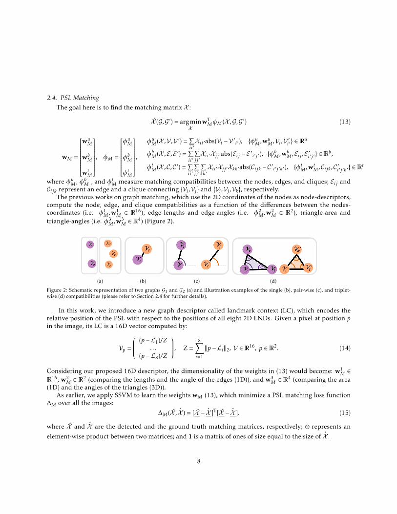
Figure 2: Schematic representation of two graphs G1 and G2 (a) and illustration examples of the single (b), pair-wise (c), and triplet-wise (d) compatibilities (please refer to Section 2.4 for further details).

In this work, we introduce a new graph descriptor called landmark context (LC), which encodes therelative position of the PSL with respect to the positions of all eight 2D LNDs. Given a pixel at position pin the image, its LC is a 16D vector computed by:

Vp =

(p −L1)/Z. . .

(p −L8)/Z

, Z =8∑i=1

‖p −Li‖2, V ∈R16, p ∈R2. (14)

Considering our proposed 16D descriptor, the dimensionality of the weights in (13) would become: w1M ∈

R16, w2

M ∈ R2 (comparing the lengths and the angle of the edges (1D)), and w3

M ∈ R4 (comparing the area

(1D) and the angles of the triangles (3D)).As earlier, we apply SSVM to learn the weights wM (13), which minimize a PSL matching loss function

∆M over all the images:

∆M (X ,∗X ) = [X −

∗X ]T[X −

∗X ]. (15)

where X and∗X are the detected and the ground truth matching matrices, respectively; � represents an

element-wise product between two matrices; and 1 is a matrix of ones of size equal to the size of∗X .

8

2.5. Adaptive Parameter Estimation for PSL Matching

There are different selection options for∗X and X in (15): (i) PSLs of the most similar subject(s) in the

training stage (to find the closest pairs, we calculate the similarity between the graphs as a function of thedifference between the PSLs, the sparsity of the PSLs, and the ratio of the eigenvalues of the covariancematrix of the coordinates) (ii) PSLs of all the images in the training data; (iii) PSLs and LNDs of the imagesin the training data; (iv) LNDs in the training data; and (v) LNDs of the test images (subject-specific).

The experimental results in Section 3 indicate that the last option (v), on-the-fly learning, is more usefulthan offline learning (options i-iv) only when LND detection is sufficiently accurate. In the on-the-flylearning option, the training data is created automatically from a novel image. Therefore, we learn topredict, for a novel image, the error in the detected positions of the LNDs (as explained next) then use thepredicted error to automatically activate the on-the-fly learning of wM in (13).

2.6. LND Error PredictionThe goal here is to calculate, for a novel image, the error in the detected positions of the LNDs. Clearly,

calculating the exact error requires the knowledge of a ground truth location. The idea here is to learn,from a training set, to predict the error using the following formulation:

∆L(L,I ) = wTEφE(L,I ) (16)

wE = [woE ...w

27E ], φE(L,I ) = [S(L) φoL(L,I ) ∇φoL(L,I )T... φ8

L(L,I ) ∇φ8L(L,I )T]

where ∆L is the estimated error given the estimated locations L; S(L) is an asymmetry feature that mea-sures the difference between the edges connecting the left neck, shoulder, armpit, and hip points and theircorresponding edges on the right side; φiL(L,I ) are the energy terms of the LND cost function in (1); ∇ is agradient operator:

∇φiL(Li ,I ) = [∂φiL(Li ,I )

∂x

∂φiL(Li ,I )∂y

]T

∇φoL(L) =∑ij

∇φoL(Li ,Lj ) =∑ij

C−1ij (Lij −

¯Lij )

We use these features to quantify the uncertainty in the probabilistic solution. It has been shown thatthe presence of uncertainty may indicate errors in the solution and this uncertainty can be quantified usingthe slope of each energy term (measured by their gradients) at the computed solution [47].

In a training stage, we calculate wE knowing ∆L(L) = ∆L(L,∗L) (6) and φE . In the testing stage, given

a predicted error ∆L(L) with low values, we perform the on-the-fly learning on the weights of the PSLmatching algorithm, otherwise, we use the off-line learnt weights.

3. Results

We evaluated our method on 194 digital color images (97 pairs, i.e. two images per subject) of thehuman back with isotropic resolution of 0.25 mm/pixel [48].

We manually prepared ground truth for the locations of both the LNDs and PSLs in all the 97x2=194images as well as their correspondences across each pair. We annotated one point (coordinate) per LNDand PSL. We had eight LNDs in each image but the number of PSLs varied between 2 and 30 (9±8).

9

Figure 3: Post-processing to refine the manual PSL locations (red markers) by relocating them to the mass centers (green markers) ofthe blobness response patches around the annotated pixels (Section 3). The top row shows the image patches (centered at the positionsof the red markers) and the bottom row shows the blobness responses.

Since the manual localization of the PSLs did not fall exactly in the centre of the PSL, we resort toan automatic post-processing step to refine the manual PSL coordinates such that it coincides with (or isrelocated to) the “centre of mass” (CoM) of the PSL. In particular, the CoM is calculated for a blobnessresponse (calculated as in [45]) patch of size 30×30 pixel centered around the annotated point (Figure 3).

Ten-fold cross-validation was performed for learning the hyperparameters of our objective functionsfor LND detection (1), PSL detection (11), and PSL matching (13). For each of the 10 validation runs, 20images (10 pairs) were left for testing and the remaining images were used for training.

Note that the images in our dataset were taken from the patients in a similar posture and within asimilar distance from the camera. Therefore, we had this underlying assumption that all the images areroughly in the same scale and orientation. This assumption mainly affects the LND detection step, which issolved by applying the pictorial algorithm [39]. This LND detection step, while not invariant to scale androtation, is robust to small changes to those pose factors [39].

Samples of qualitative results of the detected LNDs, PSLs, and PSL correspondences are shown in Figure4. In the following, we report the quantitative results of the different steps. Note that the results from[49, 13] were obtained by re-implementing the methods from the published papers.

3.1. LND DetectionCompared with our previous work reported in [5, 6], the current method detected LNDs fully auto-

matically. We achieved an average of 10.76±12.43 mm Euclidean distance error with respect to the groundtruth over 1552 LNDs in 97 image pairs (8 LNDs/image). Note that an error of ∼1 cm falls within thetypical localization variability amongst human observers [50]. In Figure 5, we show the cumulative rootmean square error (CRMSE) of the detected LNDs; CRMSE is a function that measures percentage of im-ages having LND detection error less than a specific value, e.g.: given N images in the test-stage, CRMSEof the ith LND, i = 1...8, with LND detection error ≤ z, CRMSE is defined as:

CRMSEi(z) =

N∑k=1

δ(∆L(Lki ,

∗Lki ) < z

)N

× 100%, δ(.) ={

1 if ∆ki ≤ z0 if ∆ki > z

(17)

In Figure 5, it can be seen that using SSVM to learn wL ∈ R9 produces better results than SSVM-learningof only two weights (one for the regularization and another equal weight for all data terms), i.e. wL ∈R

2 (Figure 5). Note that when equal weights are used for all (regularization and data) terms, we obtainunusable results, which are not included in Figure 5.

10

+: GT LNDx: Detected LND

GT

Hessian based

Lee et al.

GT

16DLC

2DSNC

+: GT LNDx: Detected LND

GT

Hessian based

Lee et al.

GT

16DLC

2DSNC

(a) LND detection (b) PSL detection (c) PSL Matching

Figure 4: Sample qualitative results (see text for quantitative results): (a) Detected landmarks (red) using the graphical models (Section2.1) compared with the ground truth (green). (b) Detected PSLs using the Hessian based features (red) and the method in [13] (yellow)compared with the ground truth (green). (c) PSL matching results using the 16DLC (red) and 2DSNC (yellow) descriptors comparedwith the ground truth (green) (Section 2.4).

3.2. PSL DetectionWe validate the goodness of the detected PSLs in terms of true positive fraction (TPF) and positive

predictive value (PPV) computed as the following:

TPF =(Number of true positives)/(Number of true positives + Number of false negatives) (18)

PPV =(Number of true positives)/(Number of true positives + Number of false positives).

Averaged over all the images, using the Hessian based features, we achieve TPF of 0.80±0.06 and PPVof 0.87±0.01, which outperform state-of-the-art [13] (TPF=0.68±0.18 and PPV= 0.61±0.01). Note that weconsider a detected PSL as a true positive if there is an overlap of at least 5 mm2 between the region of thedetected PSL and a ground truth.

Note that [13] does not require training data (although it had hyperparameters that were empiricallyset by hand).

3.3. Structured Parameter EstimationFigure 7(a) shows the PSL matching errors resulting from applying the different weight-learning options

(Section 2.2). First, it can be seen that considering any of the SSVM-based learnt weights drops the matchingerror from about 0.3 to 0.1 (i.e. by 66.7%) compared with the non-learnt weights (e.g. equal weights).Second, the results indicate that, given a good enough estimation of the position of the LNDs, less than20 mm (Figure 7(a)), learning the weights based on the automatically detected LNDs of the same subject(i.e. on-the-fly training) is more accurate and with less variability than using PSLs/LNDs from differentsubjects (off-line training).

In contrast to the earlier works on graph matching (Table 1), our PSL matching technique uses the threeterms (unary, binary, ternary) together

11

Lef

t Y

-ax

is:

% o

f Im

ages

Rig

ht Y

-ax

is:

% o

f Im

pro

vem

ent

0

9

50 50 0 5050 000

0

9

X-axis: in mm

Learning in

Learning in

Figure 5: Cumulative RMSE of the eight detected LNDs when learning a single weight for all data terms, i.e. wL ∈ R2 for data andregularization (dashed curves) and when learning the weights for the regularization and all the 8 data terms, i.e. wL ∈ R

9 (solidcurves) using SSVM (1); the left y-axis represents percentage of images. The colored bars on the right-side of each figure representpercentage of the improvement (read of the right y-axis) resulting from the learnt parameters compared with non-learnt. X-axis is theLND detection error computed ((16)).

CVPR09 PAMI11 MICCAI12 CVPR13

0.05

0.1

0.15

2DSNC

16DLC

(a)

AdaptiveOn−the−fly

0.06

0.13

(b)

Figure 6: (a) PSL matching error when using 2DSNC (gray bars) and 16DLC (green bars). (b) PSL matching errors resulting fromoff-line (using LNDs), on-the-fly, and adaptive learning.

3.4. LND Context EffectivenessFigure 6(a) shows the PSL matching errors ∆M (15) of the following matching algorithms: CVPR09 [6],

PAMI11 [37], MICCAI12 [5], and CVPR13 [49] using 2D spatially normalized coordinates (2DSNC) [6] andour proposed 16DLC (14). In summary, all these matching methods can be implemented by setting theobjective matching functions including binary or ternary terms and applying different optimization ap-proaches mentioned in Table 1. As it can be seen in Figure 6(a), applying 16DLC reduces the PSL matchingerror for all methods.

Note that in our previous works [5, 6, 50], we examined two other node descriptors: shape context[27] and Voronoi area [4]. The PSL matching performance resulting from applying these descriptors toour dataset was unacceptable for the following reasons. Our PSL matching problem can be consideredas a sparse graph matching problem as the PSLs are not too dense. However, shape context relies onconstructing a log-polar histogram from a dense set of points. Voronoi area descriptor, on the other hand,proved to be a weak descriptor for either sparse or dense graph matching because any points can havesimilar Voronoi areas in the presence of dense points. Further, in the presence of outliers (e.g the presence ofnewly appearing and disappearing PSLs in our work), two corresponding points could have totally differentVoronoi areas.

3.5. LND Error PredictionFigure 7(b) shows a scatter plot of the real and the predicted LND-error, which have a statistically

significant (p-value≤0.01) correlation coefficient ρ =0.61.

12

5 10 15 20 25 30 35 40 45 50

0.05

0.1

0.15

0.2

0.25

0.3

0.35

RMSE of Detected LNDs (in mm)

PS

L M

at

ch

ing

Err

o r

No learningLearn: closest graphsLearn: PSLs in trainingLearn: PSLs+LNDs in trainingLearn: LNDs in trainingLearn: LNDs in test (on−the−fly)

On-the-fly learning Off-line learning

(a)

0 300

30 ρ =0.61

Real Matching Error

Predicted Error

(b)

AdaptiveOn−the−fly

0.06

0.13

(c)

Figure 7: (a) The PSL Matching error over the RMSE of the detected LNDs without and with applying the different learning ap-proaches to learn wM ∈ R37 weights in (13). (b) Scatter plot between the real and the predicted LND-errors. (c) PSL matching errorsresulting from off-line (using LNDs), on-the-fly, and adaptive learning.

3.6. Adaptive Learning EffectivenessComparing the PSL matching errors resulting from on-the-fly and adaptive learning in Figure 7(c)

demonstrates the advantage of the adaptive approach.

4. Conclusion

We presented an end-to-end automatic PSL-tracking system, which is important for early skin cancerdetection. Our results demonstrate that the accuracy of the LND detection with SSVM-based parameterlearning is similar to experts’ annotations; the PSL detection accuracy outperforms the state-of-the-artmethods; and the new PSL descriptor with the adaptive structured on-the-fly learning gives superior PSLmatching results. During the development, we also made the following computational contributions: i)LND detection based on a structured graphical model, ii) polygon-constrained PSL detection, iii) a newgraph descriptor we call landmark context; iv) structured subject-specific hyperparameter estimation forPSL matching; and v) LND error prediction for adaptive PSL matching. All of these contributions werevalidated and shown to improve performance.

As future work, we also consider jointly solving the above mentioned problems of PSL detection andmatching. It is possible to consider the PSL detection and matching steps as two interrelated problems, andsome feedback between the matching and detection process could increase the accuracy of both individualsteps.

One of the weaknesses of our SSVM and other machine-learning approacheS for setting hyperparame-ters is that they require training data [51]. For future work, it may be interesting to see how such parametersmay be set automatically (or at least reduce the amount of annotation the user needs to make), either byusing contextual data from the images themselves, e.g. by automatically increasing regularization whenthe quality of the novel image worsens, as done in [52]. It should be noted, however, that once the methodis trained, it can operate automatically and report uncertainty in the produced results. The user can thenexamine these results quickly (especially those highly uncertain ones) and approve or correct them; thuscreating training data that can be used to re-train and improve the method.

13

Another limitation of our method is that it is not completely invariant to pose. Finding the globallyoptimal solution for fitting a deformable template (or atlas) or statistical shape model, with unknown pose(scale, rotation, and translation) remains an unsolved problem, despite recent progress [53, 54, 55]

Acknowledgements

This work was supported in part by a scholarship from Canadian Institutes of Health Research (CIHR) SkinResearch Training Centre and by grants from the Natural Sciences and Engineering Research Council ofCanada (NSERC) and Canadian Dermatology Foundation.

[1] American cancer society (2009). cancer facts and figures 2009, american cancer society. 2009. Atlanta, USA.

[2] RP. Gallagher and DI. McLean. The epidemiology of acquired melanocytic nevi- a brief review. DermatologicClinics, 13(3):595–603, 1995.

[3] J. Gachon, P. Beaulieu, J. Sei, J. Gouvernet, J. Claudel, and M. Lemaitre M. Richard J. Grob. First prospective studyof the recognition process of melanoma in dermatological practice. Arch Dermatol, 141(434–448):4, 2005.

[4] H. Huang and P. Bergstresser. A new hybrid technique for dermatological image registration. IEEE BIBE, pages1163–1167, 2007.

[5] H. Mirzaalian, T. Lee, and G. Hamarneh. Uncertainty-based feature learning for skin lesion matching using a highorder mrf optimization framework. volume 7511, pages 98–105, 2012.

[6] H. Mirzaalian, G. Hamarneh, and T.K. Lee. Graph-based approach to skin mole matching incorporating template-normalized coordinates. IEEE CVPR, pages 2152–2159, 2009.

[7] M.P. Segundo, C. Queirolo, O.R.P. Bellon, and L. Silva. Automatic 3D facial segmentation and landmark detection.pages 431 –436, 2007.

[8] P. Perakis, G. Passalis, T. Theoharis, and I. A. Kakadiaris. 3D facial landmark detection and face registration. 2010.

[9] V. Potesil, T. Kadir, G. Platsch, and S. Brady. Personalization of pictorial structures for anatomical landmarklocalization. IPMI, pages 333–345, 2011.

[10] C. Chenaand W. Xiea, J. Frankeb, P. Grutznerb, L. Noltea, and G. Zheng. Automatic x-ray landmark detection andshape segmentation via data-driven joint estimation of image displacements. MIA, pages 1–13, 2014.

[11] T. Sang, W. Freeman, and H. Tsao. A reliable skin mole localization scheme. IEEE ICCV, pages 1 –8, 2007.

[12] J.S. Pierrard and T. Vetter. Skin detail analysis for face recognition. IEEE CVPR, pages 1–8, 2007.

[13] T. K. Lee, M.S. Atkins, M.A. King, S. Lau, and D.I. McLean. Counting moles automatically from back images. IEEETBE, 52(11):1966 –1969, nov. 2005.

[14] S. Gold and A. Rangarajan. A graduated assignment algorithm for graph matching. IEEE PAMI, 18(4):377–388,1996.

[15] C. Berg, L. Berg, and J. Malik. Shape matching and object recognition using low distortion correspondence. IEEECVPR, pages 26–33, 2005.

[16] M. Leordeanu, A. Zanfir, and C. Sminchisescu. Semi-supervised Learning and Optimization for HypergraphMatching. IEEE ICCV, 2011.

14

[17] L. Torresani, V. Kolmogorov, and C. Rother. Feature correspondence via graph matching: Models and globaloptimization. ECCV, 5303:596–609, 2008.

[18] Y. Zeng, C. Wang, W. Yang, X. Gu, D. Samaras, and N. Paragios. Dense non-rigid surface registration using high-order graph matching. IEEE CVPR, pages 382–389, 2010.

[19] N. Ansari, M.-H. Chen, and E.S.H. Hou. Point pattern matching by a genetic algorithm. In IEEE IECON, volume 2,pages 1233–1238, 1990.

[20] M. Tico and C. Rusu. Point pattern matching using a genetic algorithm and Voronoi tessellation. EUSIPCO, pages1589–1592, 1998.

[21] L. Zhang, W. Xu, and C. Chang. Genetic algorithm for affine point pattern matching. Pattern Recognition Letters,24:9–19, 2010.

[22] C. Xing, W. Wei, J. Wu, C. Zhang, and Y Zhou. Matching point pattern using a munkres genetic algorithm. Journalof Convergence Information Technology, 6(12):376–383, 2011.

[23] Z. Zhang. Iterative point matching for registration of free-form curves and surfaces. IJCV, 13:119–152, 1994.

[24] A. Myronenko, X. Song, and M. Carreira-Perpinan. Non-rigid point set registration: Coherent point drift. InB. Scholkopf, J. Platt, and T. Hoffman, editors, NIPS, pages 1009–1016. MIT Press, 2007.

[25] S. Gold, A. Rangarajan, C. Lu, and E. Mjolsness. New algorithms for 2d and 3d point matching: Pose estimationand correspondence. Pattern Recognition, 31:957–964, 1998.

[26] B. Jian and B. Vemuri. A robust algorithm for point set registration using mixture of gaussians. IEEE ICCV,2:1246–1251, 2005.

[27] S. Belongie, J. Malik, and J. Puzicha. Shape matching and object recognition using shape contexts. IEEE PAMI,24(4):509–522, 2002.

[28] Y. Zheng and M.D. Doermann. Robust point matching for nonrigid shapes by preserving local neighborhoodstructures. IEEE PAMI, 28(4):643, 2006.

[29] H. Chui and A. Rangarajan. A new point matching algorithm for non-rigid registration. Comput. Vis. ImageUnderst., 89:114–141, 2003.

[30] F. Escolano, E. Hancock, and M. Lozano. Graph matching through entropic manifold alignment. IEEE CVPR,pages 2417 –2424, 2011.

[31] B. Wyk and M. Wyk. A pocs-based graph matching algorithm. IEEE PAM, 26(11):526–530, 2004.

[32] R. Zass and A. Shashua. Probabilistic graph and hypergraph matching. IEEE CVPR, pages 1–8, 2008.

[33] M. Leordeanu and M. Hebert. A spectral technique for correspondence problems using pairwise constraints. IEEEICCV, 2:1482–1489, 2005.

[34] T. Cour, . Srinivasan, and J. Shi. Balanced graph matching. NIPS, pages 1–8, 2006.

[35] Marius Leordeanu, Rahul Sukthankar, and Martial Hebert. Unsupervised learning for graph matching. IJCV,pages 1–18, 2011.

[36] T. Caetano, J. McAuley, Cheng Q., and A. Smola. Learning graph matching. IEEE PAMI, 31(6):1048 –1058, june2009.

15

[37] O. Duchenne, F. Bach, I. Kweon, and J. Ponce. A tensor-based algorithm for high-order graph matching. IEEETPAMI, 1(99):1–13, 2011.

[38] M. Chertok and Y. Keller. Efficient high order matching. IEEE PAMI, 32(12):2205 –2215, 2010.

[39] Pedro F. Felzenszwalb and Daniel P. Huttenlocher. Pictorial structures for object recognition. Int. J. Comput.Vision, 61(1):55–79, January 2005.

[40] T. Joachims, T. Finley, and C. Yu. Cutting-plane training of structural SVMs. Machine Learning, pages 27–59, 2009.

[41] Douglas A. Perednia and Raymond G. White. Automatic registration of multiple skin lesions by use of pointpattern matching. CMIG, 16(3):205 – 216, 1992.

[42] Juha Roning and Marcel Riech. Registration of nevi in successive skin images for early detection of melanoma.IEEE ICPR, 1:352–357, 1998.

[43] L. Breiman. Random forests. Machine Learning, pages 5–32, 2001.

[44] T. Ojala, M. Pietikinen, and D. Harwood. Performance evaluation of texture measures with classification based onkullback discrimination of distributions. ICPR, 1:582–585, 1994.

[45] K. L. Vincken A. Frangi, W. J. Niessen and M. A. Viergever. Multiscale vessel enhancement filtering. ICPR,1:130–137, 1998.

[46] J. Friedman. Greedy function approximation: A gradient boosting machine. Annals of Statistics, 29:1189–1232,2000.

[47] T. Kohlberger, V. Singh, C. Alvino, C. Bahlmann, and L. Grady. Evaluating segmentation error without groundtruth. MICCAI, pages 528–536, 2012.

[48] R. Gallagher, J. Rivers, T.K. Lee, C.D. Bajdik, David I. McLean, and A.J. Coldman. Broad-Spectrum SunscreenUse and the Development of New Nevi in White Children: A Randomized Controlled Trial. JAMA, 283(22):2955–2960, 2000.

[49] N. Hu, R. Rustamov, and L. Guibas. Graph matching with anchor nodes: A learning approach. IEEE CVPR, pages2906–2913, 2013.

[50] H. Mirzaalian, T. K. Lee, and G. Hamarneh. Spatial normalization of human back images for dermatologicalstudies. IEEE JBHI, pages 1–13, 2013.

[51] C. Wang, N. Komodakis, and N. Paragios. Markov random field modeling, inference and learning in computervision and image understanding: A survey. Computer Vision and Image Understanding, 117(11):1610–1627, 2013.

[52] J. Rao, R. Abugharbieh, and G. Hamarneh. Adaptive regularization for image segmentation using local imagecurvature cues. ECCV, pages 651–665, 2010.

[53] C. Wang, O. Teboul, F. Michel, S. Essafi, and N. Paragios. 3D knowledge-based segmentation using pose-invarianthigher-order graphs. MICCAI, 6363:189–196, 2010.

[54] D. Cremers, F. R. Schmidt, and F. Barthel. Shape priors in variational image segmentation: Convexity, lipschitzcontinuity and globally optimal solutions. IEEE CVPR, pages 1–6, 2008.

[55] S. Andrews, C. McIntosh, and G. Hamarneh. Convex multi-region probabilistic segmentation with shape prior inthe isometric logratio transformation space. IEEE ICCV, 8673:2096–2103, 2011.

16