Embed Size (px)
Citation preview
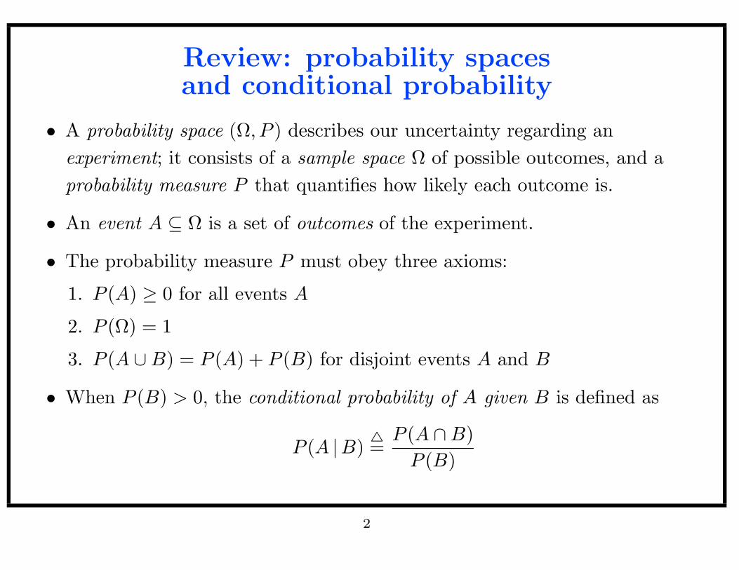
Review: probability spacesand conditional probability
• A probability space (Ω, P ) describes our uncertainty regarding an
experiment; it consists of a sample space Ω of possible outcomes, and a
probability measure P that quantifies how likely each outcome is.
• An event A ⊆ Ω is a set of outcomes of the experiment.
• The probability measure P must obey three axioms:
1. P (A) ≥ 0 for all events A
2. P (Ω) = 1
3. P (A ∪B) = P (A) + P (B) for disjoint events A and B
• When P (B) > 0, the conditional probability of A given B is defined as
P (A |B)4=P (A ∩B)
P (B)
2
Review: random variables and densities
• A random variable X : Ω → Ξ picks out some aspect of the outcome.
• The density pX : Ξ → < describes how likely X is to take on certain values.
• We usually work with a set of random variables and their joint density; the
probability space is implicit.
• The two types of densities suitable for computation are table densities (for
finite-valued variables) and the (multivariate) Gaussian (for real-valued
variables).
• Using a joint density, we can compute marginal and conditional densities
over subsets of variables.
• Inference is the problem of computing one or more conditional densities
given observations.
3
Independence
• Two events A and B are independent iff
P (A) = P (A |B)
or, equivalently, iff
P (A ∩B) = P (A) × P (B)
Note that this definition is symmetric.
• If A and B are independent, learning that B happened does not make A
more or less likely to occur.
• Two random variables X and Y are independent if for all x and y
pX(x) = pX|Y (x, y)
In this case we write X⊥⊥Y . Note that this corresponds to (perhaps
infinitely) many event independencies.
4
Example of independence
• Let’s say our experiment is to flip two fair coins. Our sample space is
Ω = (heads, heads), (heads, tails), (tails, heads), (tails, tails)
and P (ω) = 14
for each ω ∈ Ω.
• The two events
A = (heads, heads), (heads, tails)
B = (heads, heads), (tails, heads)
are independent, since P (A ∩B) = P (A) × P (B) = 14.
5
Example of non-independence
• If our experiment is to draw a card from a deck, our sample space is
Ω = A♥, 2♥, . . . ,K♥,A♦, 2♦, . . . ,K♦,A♣, 2♣, . . . ,K♣,A♠, 2♠, . . . ,K♠
Let P (ω) = 152
for each ω ∈ Ω.
• The random variables
N(ω) =
n if ω is the number n
0 otherwise
F (ω) =
true if ω is a face card
false otherwise
are not independent, since
4
52= pN (3) 6= pN |F (3, true) = 0
6
Independence is rare in complex systems
• Independence is very powerful because it allows us to reason about aspects
of a system in isolation.
• However, it does not often occur in complex systems. For example, try and
think of two medical symptoms that are independent.
• A generalization of independence is conditional independence, where two
aspects of a system become independent once we observe a third aspect.
• Conditional independence does often arise and can lead to significant
representational and computational savings.
7
Conditional independence
• Let A, B, and C be events. A and B are conditionally independent given C
iff
P (A |C) = P (A |B ∩ C)
or, equivalently, iff
P (A ∩B |C) = P (A |C) × P (B |C)
• If A and B are conditionally independent, then once we learn C, learning
B gives us no additional information about A.
• Two random variables X and Y are conditionally independent given Z if
for all x, y, and z
pX|Z(x, z) = pX|Y Z(x, y, z)
In this case we write X⊥⊥Y |Z. This also corresponds to (perhaps
infinitely) many event conditional independencies.
8
Common sense examplesof conditional independence
Some examples of conditional independence assumptions:
• The operation of a car’s starter motor and its radio are conditionally
independent given the status of the battery.
• The GPA of a student and her SAT score are conditionally independent
given her intelligence.
• Symptoms are conditionally independent given the disease.
• The future and the past are conditionally independent given the present.
This is called the Markov assumption.
An intuitive test of X⊥⊥Y |Z:
Imagine that you know the value of Z and you are trying to guess the
value of X. In your pocket is an envelope containing the value of Y .
Would opening the envelope help you guess X? If not, then X⊥⊥Y |Z.
9
Example: the burglary problem
• Let’s say we have a joint density over five random variables:
1. E ∈ true, false: Has an earthquake happened? Earthquakes are
unlikely.
2. B ∈ true, false: Has a burglary happened? Burglaries are also
unlikely, but more likely than earthquakes.
3. A ∈ true, false: Did the alarm go off? The alarm is usually tripped by
a burglary, but an earthquake can also make it go off.
4. J ∈ true, false: Did my neighbor John call me at work? John will call
if he hears the alarm, but he often listens to music on his headphones.
5. M ∈ true, false: Did my neighbor Mary call me at work? Mary will
call if she hears the alarm, but she also calls just to chat.
• I’ve just found out that John called. Has my house been burglarized?
• Problem: compute pB|J(·, true) from the joint density pEBAJM .
10
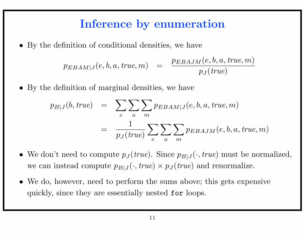
Inference by enumeration
• By the definition of conditional densities, we have
pEBAM |J(e, b, a, true,m) =pEBAJM (e, b, a, true,m)
pJ(true)
• By the definition of marginal densities, we have
pB|J(b, true) =∑
e
∑
a
∑
m
pEBAM |J(e, b, a, true,m)
=1
pJ(true)
∑
e
∑
a
∑
m
pEBAJM (e, b, a, true,m)
• We don’t need to compute pJ(true). Since pB|J(·, true) must be normalized,
we can instead compute pB|J(·, true) × pJ(true) and renormalize.
• We do, however, need to perform the sums above; this gets expensive
quickly, since they are essentially nested for loops.
11
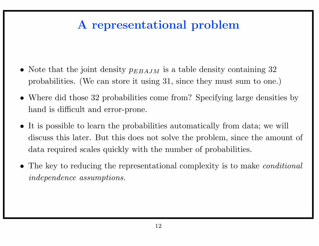
A representational problem
• Note that the joint density pEBAJM is a table density containing 32
probabilities. (We can store it using 31, since they must sum to one.)
• Where did those 32 probabilities come from? Specifying large densities by
hand is difficult and error-prone.
• It is possible to learn the probabilities automatically from data; we will
discuss this later. But this does not solve the problem, since the amount of
data required scales quickly with the number of probabilities.
• The key to reducing the representational complexity is to make conditional
independence assumptions.
12
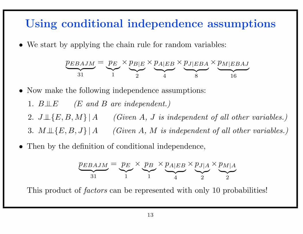
Using conditional independence assumptions
• We start by applying the chain rule for random variables:
pEBAJM︸ ︷︷ ︸
31
= pE︸︷︷︸
1
× pB|E︸︷︷︸
2
× pA|EB︸ ︷︷ ︸
4
× pJ|EBA︸ ︷︷ ︸
8
× pM |EBAJ︸ ︷︷ ︸
16
• Now make the following independence assumptions:
1. B⊥⊥E (E and B are independent.)
2. J⊥⊥E,B,M |A (Given A, J is independent of all other variables.)
3. M⊥⊥E,B, J |A (Given A, M is independent of all other variables.)
• Then by the definition of conditional independence,
pEBAJM︸ ︷︷ ︸
31
= pE︸︷︷︸
1
× pB︸︷︷︸
1
× pA|EB︸ ︷︷ ︸
4
× pJ|A︸︷︷︸
2
× pM |A︸ ︷︷ ︸
2
This product of factors can be represented with only 10 probabilities!
13
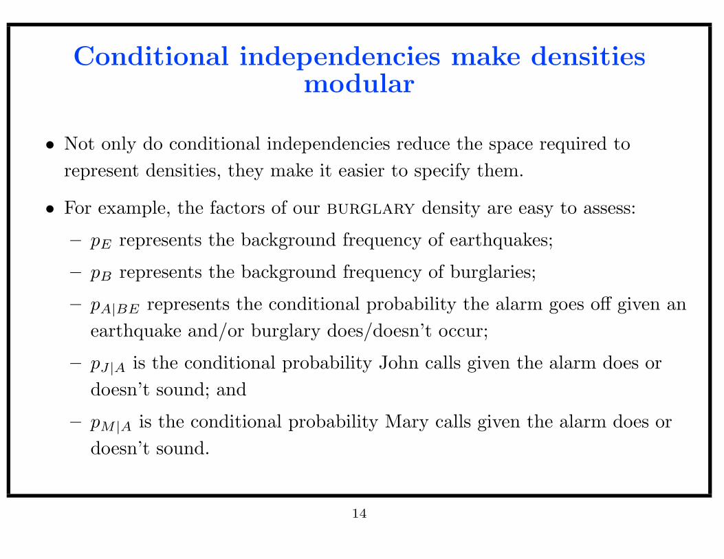
Conditional independencies make densitiesmodular
• Not only do conditional independencies reduce the space required to
represent densities, they make it easier to specify them.
• For example, the factors of our burglary density are easy to assess:
– pE represents the background frequency of earthquakes;
– pB represents the background frequency of burglaries;
– pA|BE represents the conditional probability the alarm goes off given an
earthquake and/or burglary does/doesn’t occur;
– pJ|A is the conditional probability John calls given the alarm does or
doesn’t sound; and
– pM |A is the conditional probability Mary calls given the alarm does or
doesn’t sound.
14
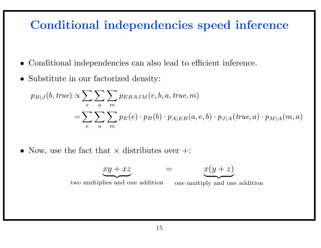
Conditional independencies speed inference
• Conditional independencies can also lead to efficient inference.
• Substitute in our factorized density:
pB|J(b, true) ∝∑
e
∑
a
∑
m
pEBAJM (e, b, a, true, m)
=∑
e
∑
a
∑
m
pE(e) · pB(b) · pA|EB(a, e, b) · pJ|A(true, a) · pM|A(m, a)
• Now, use the fact that × distributes over +:
xy + xz︸ ︷︷ ︸
two multiplies and one addition
= x(y + z)︸ ︷︷ ︸
one multiply and one addition
15
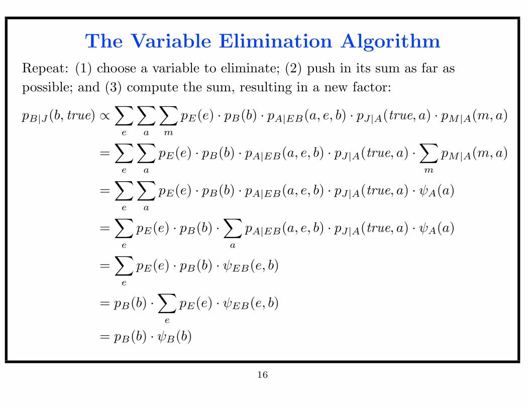
The Variable Elimination Algorithm
Repeat: (1) choose a variable to eliminate; (2) push in its sum as far as
possible; and (3) compute the sum, resulting in a new factor:
pB|J(b, true) ∝∑
e
∑
a
∑
m
pE(e) · pB(b) · pA|EB(a, e, b) · pJ|A(true, a) · pM |A(m, a)
=∑
e
∑
a
pE(e) · pB(b) · pA|EB(a, e, b) · pJ|A(true, a) ·∑
m
pM |A(m, a)
=∑
e
∑
a
pE(e) · pB(b) · pA|EB(a, e, b) · pJ|A(true, a) · ψA(a)
=∑
e
pE(e) · pB(b) ·∑
a
pA|EB(a, e, b) · pJ|A(true, a) · ψA(a)
=∑
e
pE(e) · pB(b) · ψEB(e, b)
= pB(b) ·∑
e
pE(e) · ψEB(e, b)
= pB(b) · ψB(b)
16
Complexity of Variable Elimination
• The time and space complexities of Variable Elimination are dominated by
the size of the largest intermediate factor.
• Choosing the elimination ordering that minimizes this complexity is an
NP-hard problem.
• Often, the sizes of the intermediate factors grow so large that inference is
intractable, but there are many interesting models where it does not. The
difference between these two cases lies in the independence properties.
• Graphical models are powerful tools for visualizing the independence
properties of complex probability models. There are two kinds:
– Directed graphical models (Bayesian networks)
– Undirected graphical models (Markov random fields)
17
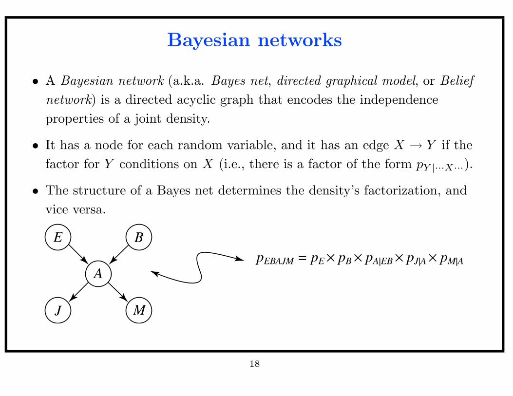
Bayesian networks
• A Bayesian network (a.k.a. Bayes net, directed graphical model, or Belief
network) is a directed acyclic graph that encodes the independence
properties of a joint density.
• It has a node for each random variable, and it has an edge X → Y if the
factor for Y conditions on X (i.e., there is a factor of the form pY |···X···).
• The structure of a Bayes net determines the density’s factorization, and
vice versa.
M
BE
A
pEBAJM = pE × pB × pA|EB × pJ|A × pM|A
J
18
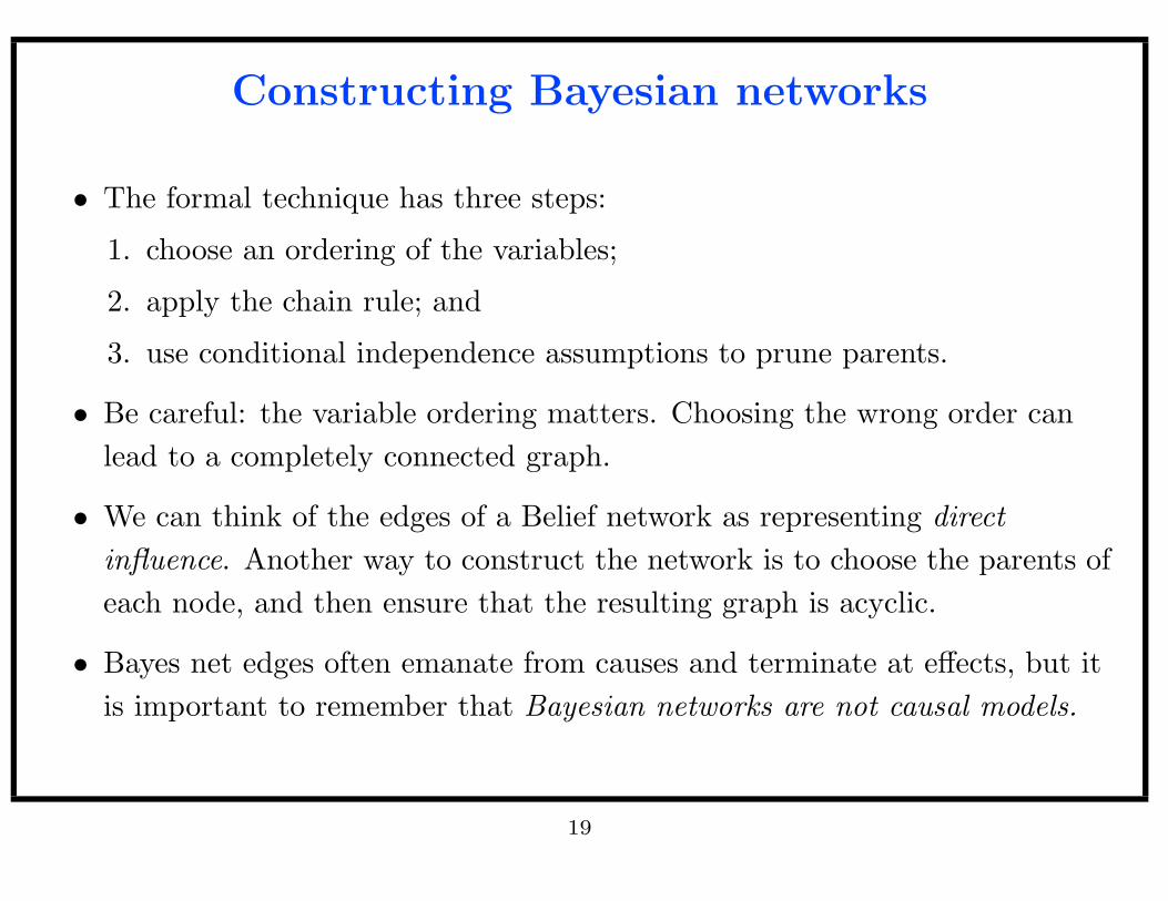
Constructing Bayesian networks
• The formal technique has three steps:
1. choose an ordering of the variables;
2. apply the chain rule; and
3. use conditional independence assumptions to prune parents.
• Be careful: the variable ordering matters. Choosing the wrong order can
lead to a completely connected graph.
• We can think of the edges of a Belief network as representing direct
influence. Another way to construct the network is to choose the parents of
each node, and then ensure that the resulting graph is acyclic.
• Bayes net edges often emanate from causes and terminate at effects, but it
is important to remember that Bayesian networks are not causal models.
19
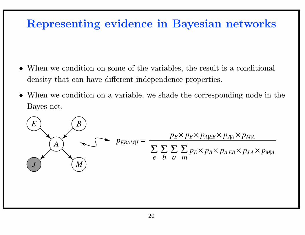
Representing evidence in Bayesian networks
• When we condition on some of the variables, the result is a conditional
density that can have different independence properties.
• When we condition on a variable, we shade the corresponding node in the
Bayes net.
M
BE
A
J
pEBAM|J =pE × pB × pA|EB × pJ|A × pM|A
Σ Σ Σ Σ pE × pB × pA|EB × pJ|A × pM|Ae b a m
20
Encoding conditional independence viad-separation
• Bayesian networks encode the independence properties of a density.
• We can determine if a conditional independence X⊥⊥Y | Z1, . . . , Zk holds
by appealing to a graph separation criterion called d-separation (which
stands for direction-dependent separation).
• X and Y are d-separated if there is no active path between them.
• The formal definition of active paths is somewhat involved. The Bayes Ball
Algorithm gives a nice graphical definition.
21
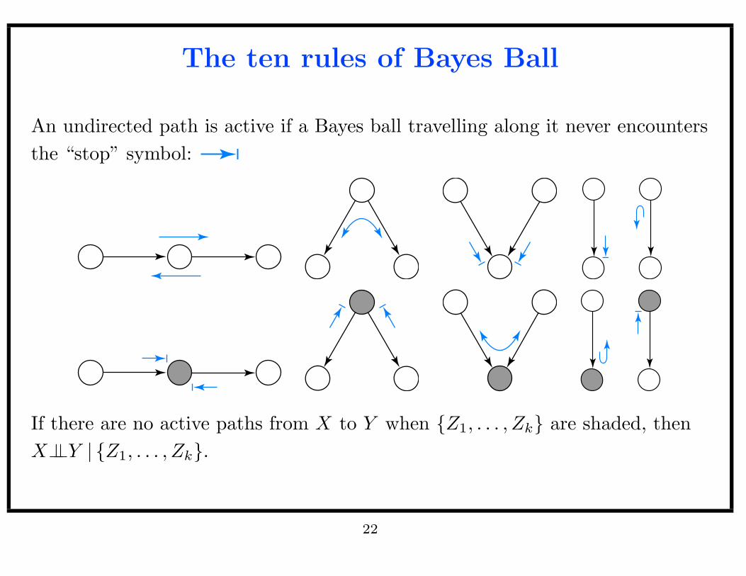
The ten rules of Bayes Ball
An undirected path is active if a Bayes ball travelling along it never encounters
the “stop” symbol:
If there are no active paths from X to Y when Z1, . . . , Zk are shaded, then
X⊥⊥Y | Z1, . . . , Zk.
22
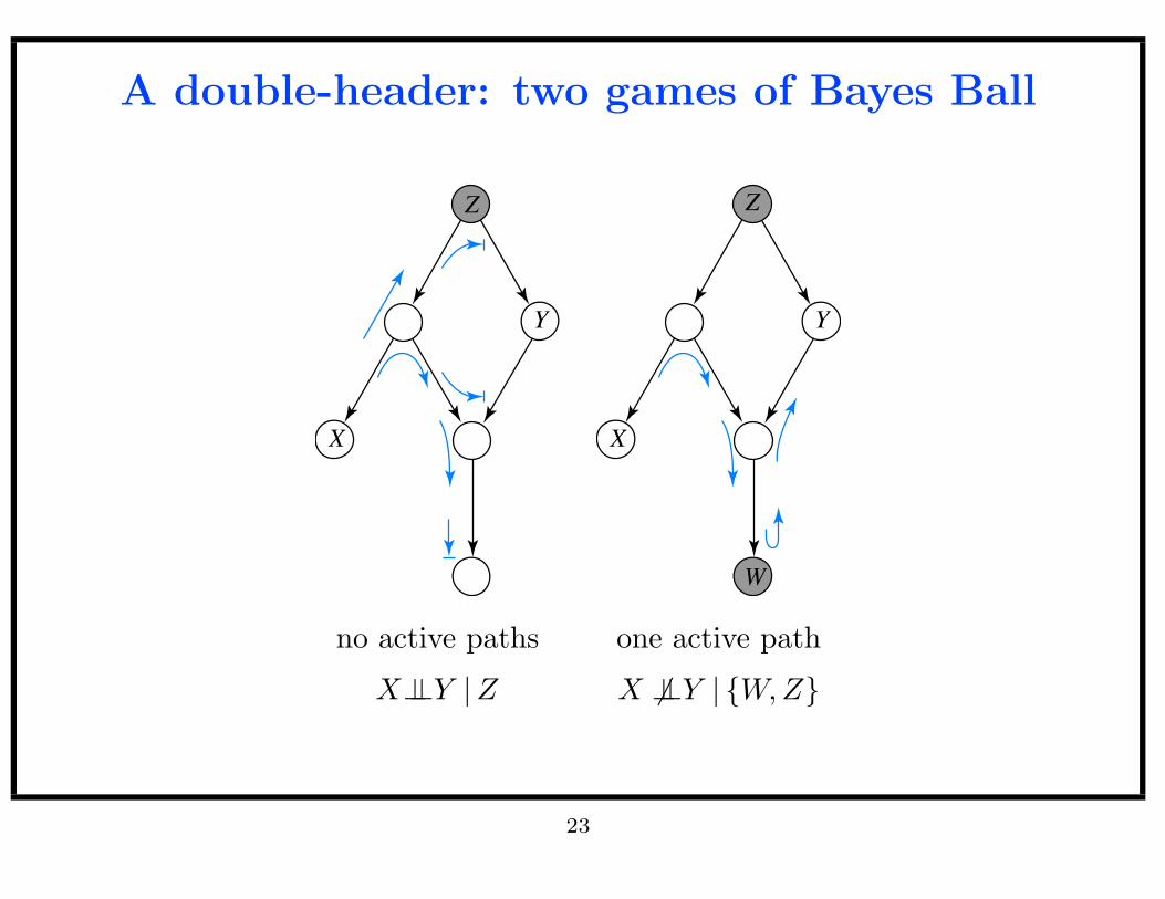
A double-header: two games of Bayes Ball
X
Y
Z
X
W
Y
Z
no active paths one active path
X⊥⊥Y |Z X 6⊥⊥Y | W,Z
23
Undirected graphical models
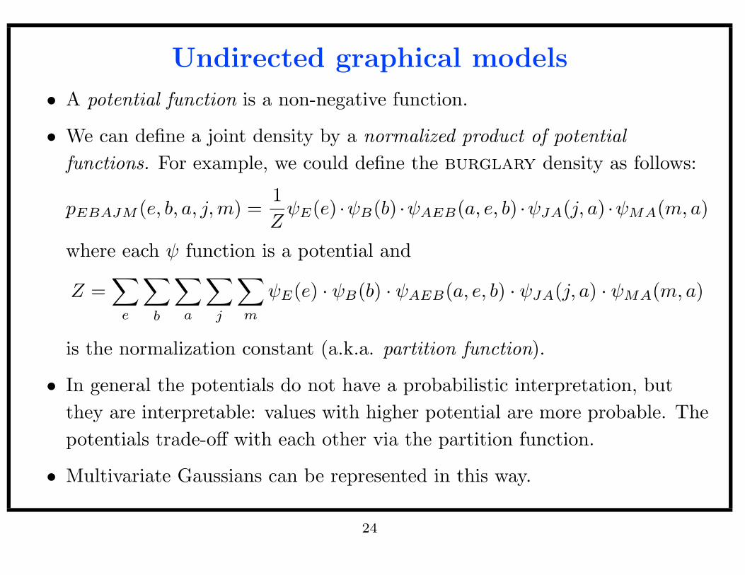
• A potential function is a non-negative function.
• We can define a joint density by a normalized product of potential
functions. For example, we could define the burglary density as follows:
pEBAJM (e, b, a, j,m) =1
ZψE(e) ·ψB(b) ·ψAEB(a, e, b) ·ψJA(j, a) ·ψMA(m, a)
where each ψ function is a potential and
Z =∑
e
∑
b
∑
a
∑
j
∑
m
ψE(e) · ψB(b) · ψAEB(a, e, b) · ψJA(j, a) · ψMA(m, a)
is the normalization constant (a.k.a. partition function).
• In general the potentials do not have a probabilistic interpretation, but
they are interpretable: values with higher potential are more probable. The
potentials trade-off with each other via the partition function.
• Multivariate Gaussians can be represented in this way.
24
Conditional independencein undirected graphical models
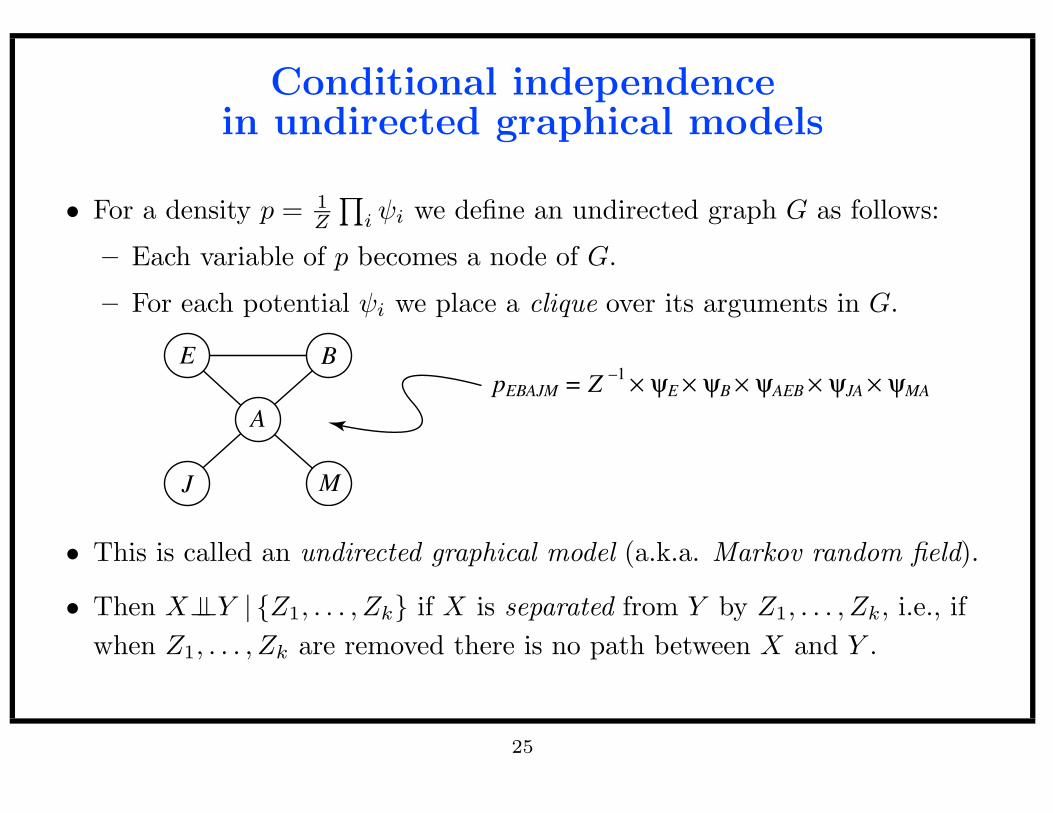
• For a density p = 1Z
∏
i ψi we define an undirected graph G as follows:
– Each variable of p becomes a node of G.
– For each potential ψi we place a clique over its arguments in G.
M
BE
A
pEBAJM = Z –1
× ψE × ψB × ψAEB × ψJA × ψMA
J
• This is called an undirected graphical model (a.k.a. Markov random field).
• Then X⊥⊥Y | Z1, . . . , Zk if X is separated from Y by Z1, . . . , Zk, i.e., if
when Z1, . . . , Zk are removed there is no path between X and Y .
25
The Hammersley-Clifford Theorem
• When p is strictly positive, the connection between conditional
independence and factorization is much stronger.
• Let G be an undirected graph over a set of random variables X1, . . . , Xk.
• Let P1 be the set of positive densities over X1, . . . , Xk that are of the
form
p =1
Z
∏
C
ψC
where each ψC is a potential over a clique of G.
• Let P2 be the set of positive densities with the conditional independencies
encoded by graph separation in G.
• Then P1 = P2.
26
Comparing directed andundirected graphical models
• Specifying an undirected graphical model is easy (normalized product of
potentials), but the factors don’t have probabilistic interpretations.
Specifying a directed graphical model is harder (we must choose an ordering
of the variables), but the factors are marginal and conditional densities.
• Determining independence in undirected models is easy (graph separation),
and in directed models it is hard (d-separation).
• Directed and undirected models are different languages: there are densities
with independence properties that can be described only by directed
models; the same is true for undirected models.
• In spite of this, inference in a directed model usually starts by converting it
into an undirected graphical model with fewer conditional independencies.
27
Moralization
• Because the factors of a Bayesian network are marginal and conditional
densities, they are also potential functions.
• Thus, a directed factorization is also an undirected factorization (with
Z = 1). Each clique consists of a variable and its parents in the Bayes net.
• We can transform a Bayesian network into a Markov random field by
placing a clique over each family of the Bayesian network and dropping the
directed edges.
• This process is called moralization because we marry (or connect) the
variable’s parents and then drop the edge directions.
28
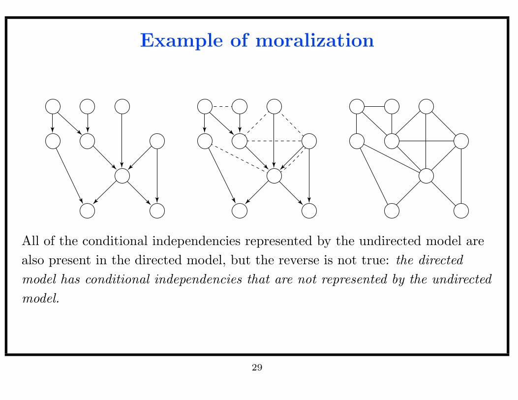
Example of moralization
All of the conditional independencies represented by the undirected model are
also present in the directed model, but the reverse is not true: the directed
model has conditional independencies that are not represented by the undirected
model.
29
Node Elimination: a graphical viewof Variable Elimination
• The intermediate factors we created in the Variable Elimination algorithm
are also potential functions.
• Thus, after each elimination step we are left with a density that can be
visualized as an undirected graphical model.
• The Node Elimination algorithm is to repeatedly:
1. choose a node (variable) to eliminate;
2. create an elimination clique (intermediate factor) from the node and its
neighbors; and
3. remove the node and its incident edges.
The result is a set of elimination cliques that represent the arguments of
the intermediate factors.
30
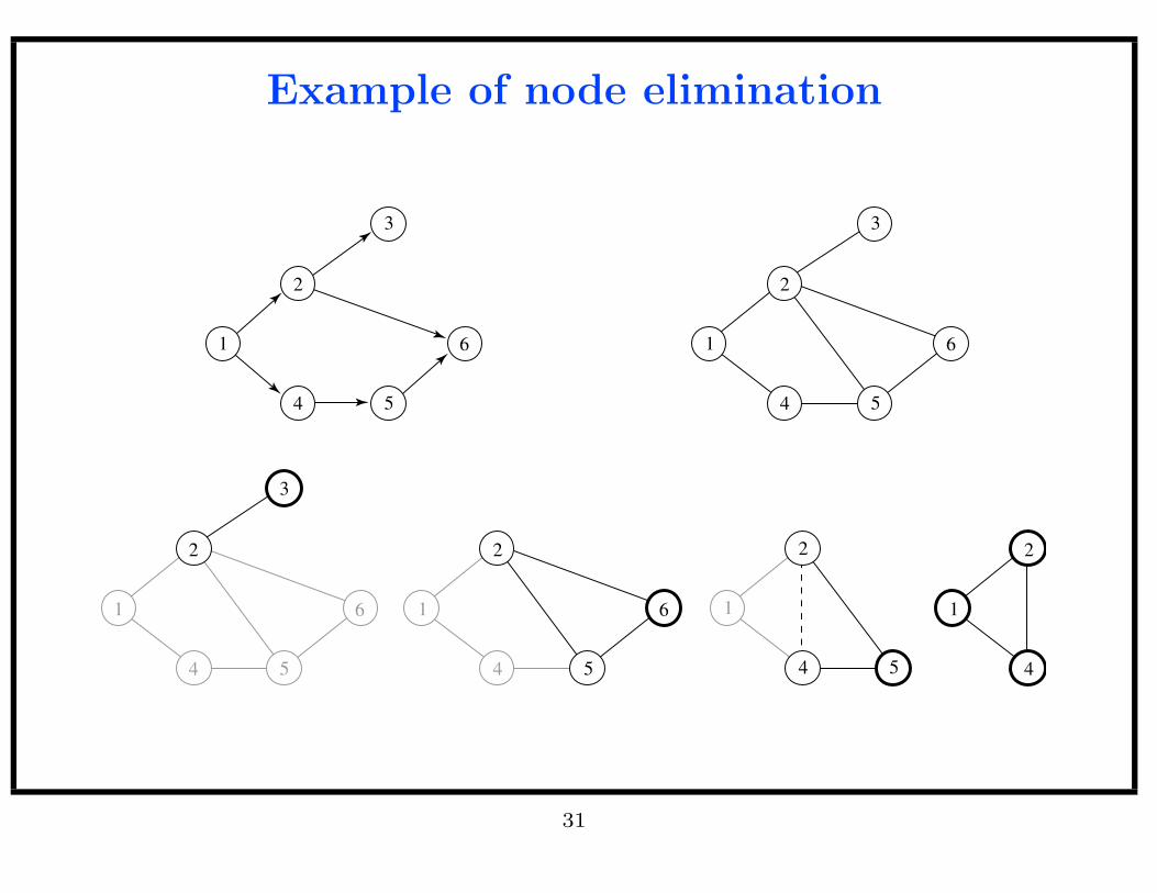
Example of node elimination
1
2
3
4 5
6 1
2
3
4 5
6
1
2
3
4 5
6 1
2
4 5
6 1
2
4 5
1
2
4
31
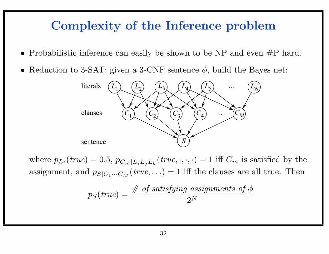
Complexity of the Inference problem
• Probabilistic inference can easily be shown to be NP and even #P hard.
• Reduction to 3-SAT: given a 3-CNF sentence φ, build the Bayes net:
L1
L2
L3
L4
L5
LN
CMC4
C3
C2
C1
S
...
...
literals
clauses
sentence
where pLi(true) = 0.5, pCm|LiLjLk
(true, ·, ·, ·) = 1 iff Cm is satisfied by the
assignment, and pS|C1···CM(true, . . .) = 1 iff the clauses are all true. Then
pS(true) =# of satisfying assignments of φ
2N
32
Looking ahead. . .
• Graphical models provide a language for characterizing independence
properties. They have two important uses:
– Representational. We can obtain compact joint densities by choosing a
sparse graphical model and then choosing its local factors.
– Computational. For example, Variable Elimination can be viewed in
terms of operations on a graphical model. This model can be used to
guide computation, e.g., it helps in choosing good elimination orders.
• Next time we will continue to explore the connection between Graph
Theory and Probability Theory to obtain
– graphical characterizations of tractable inference problems, and
– the junction tree inference algorithms.
33
Summary
• Two random variables X and Y are (marginally) independent (written
X⊥⊥Y ) iff pX(·) = pX|Y (·, y) for all y.
• If X⊥⊥Y then Y gives us no information about X.
• X and Y are conditionally independent given Z (written X⊥⊥Y |Z) iff
pX|Z(·, z) = pX|Y Z(·, y, z) for all y and z.
• If X⊥⊥Y |Z then Y gives us no additional information about X once we
know Z.
• We can obtain compact, factorized representations of densities by using the
chain rule in combination with conditional independence assumptions.
• The Variable Elimination algorithm uses the distributivity of × over + to
perform inference efficiently.
34
Summary (II)
• A Bayesian network encodes the independence properties of a density using
a directed acyclic graph.
• We can answer conditional independence queries by using the Bayes Ball
algorithm, which is an operational definition of d-separation.
• A potential is a non-negative function. One simple way to define a joint
density is as a normalized product of potential functions.
• An undirected graphical model for such a density has a clique of edges over
the argument set of every potential.
• In an undirected graphical model, graph separation corresponds to
conditional independence.
• Moralization is the process of converting a directed graphical model into an
undirected graphical model. This process does not preserve all of the
conditional independence properties.
35