Size-Dependent Policies and Firm Behavior

by

Miguel Almunia Candela

A dissertation submitted in partial satisfaction of the

requirements for the degree of

Doctor of Philosophy

in

Economics

in the

Graduate Division

of the

University of California, Berkeley

Committee in charge:

Professor Emmanuel Saez, ChairProfessor Alan AuerbachProfessor Edward MiguelProfessor Ernesto Dal Bó

Spring 2013

Size-Dependent Policies and Firm Behavior

Copyright © 2013

by

Miguel Almunia Candela

Abstract

Size-Dependent Policies and Firm Behavior

by

Miguel Almunia Candela

Doctor of Philosophy in Economics

University of California, Berkeley

Professor Emmanuel Saez, Chair

Most countries have laws that offer regulatory advantages to small firms, such as lowertaxes or more flexible labor rules. To determine what firms are eligible to these advantages,it is necessary to define what characterizes a small firm. This is usually done by specifyingthresholds in terms of the maximum number of employees, annual revenues, total assets, ora combination of all three. The existence of such thresholds gives firms incentives to strate-gically remain small to benefit from the regulatory advantages. It also provides researcherswith an opportunity to analyze the effects of those regulations, by studying the behavior offirms that are close to the eligibility cutoff.

In the first chapter, my co-author David Lopez-Rodriguez and I study the effects onfirm behavior of a discontinuity in tax enforcement intensity in Spain. The Large Taxpay-ers’ Unit (LTU), established in 1995, monitors and enforces the taxation of companies withoperating revenue above €6 million, resulting in more frequent tax audits and more infor-mation requirements for those firms. We exploit this discontinuity to estimate the impact oftax enforcement on firms’ reporting behavior, using a panel dataset of financial statementsfor Spanish firms from the period 1999-2011. We find an excess mass of firms locating,or “bunching”, just below the revenue threshold. Bunching is stronger in the boom period(1999-2007) than in the recession period (2008-2011). Based on the number of bunchingfirms, we estimate that firms reduce reported revenue by up to 7.5% in the boom period toavoid falling in the high enforcement regime. A dynamic analysis shows that firm’s revenuegrowth rates decline substantially as firms approach the LTU threshold from below, andthere is short-term persistence (up to 3 years) in bunching behavior.

In the second chapter, my co-author David Lopez-Rodriguez and I analyze whetherbunching of firms below a discontinuity in tax enforcement intensity is due to production(real) or evasion responses. Using an extended theoretical framework, we derive predictionsabout the behavior of reported input costs under the polar hypothesis of a pure real responseand a pure evasion response. We test the plausibility of the two hypotheses using graphicalevidence on the patterns of reported input costs around the LTU threshold. This evidencesuggests that bunching firms underreport their revenue, overreport their material input costs

1

and underreport their labor costs in order to evade several taxes: corporate income tax, pay-roll tax and the value added tax (VAT). We also run panel regressions with firm fixed effectswhich broadly confirm the results from the graphical analysis. Overall, the results suggestthat firms react to this tax enforcement policy mostly through changes in reporting, ratherthan changes in production. The efficiency costs of tax enforcement are thus likely to besmall because tax evasion constitutes a reallocation of income to tax-evading firms, ratherthan a net loss for society. Finally, we do a rough estimation of the upper bound of corporateincome tax evasion, which yields a modest amount of evasion.

In the third chapter, I study the impact of a set of labor regulations in France thatapplies only to firms with more than 50 employees. These regulations increase the averagelabor cost per employee, giving firms an incentive to remain small. The firm size distributionshows strong bunching below the threshold for the period 2002-2008. In terms of growthpatterns, the proportion of firms increasing their size from one year to the next drops almostby half at 49 employees, while the share of firms keeping employment constant doubles. Iset up a stylized model where firms only choose their number of employees to derive anexpression for the elasticity of labor demand, and then estimate it using the number ofbunching firms as a sufficient statistic. I obtain a point estimate of e = 0.055, which isstatistically different from zero at the 10% level. Making an adjustment for the possibilitythat some firms do not respond to the regulations due to optimization frictions, I obtaina point estimate of eF = 0.572. The latter can be interpreted as an upper bound for thelong-term structural elasticity, although it is imprecisely estimated (the standard error is0.668). These point estimates are considerably below labor demand elasticities estimated inthe literature, which according to Hamermesh (1993) tend to be in the interval (0.15, 0.75).An intuitive explanation for why I obtain low point estimates is that bunching firms maybe adjusting their production by increasing the use of other inputs instead of labor. I findsome preliminary evidence supporting this hypothesis: median fixed assets per employeedrop sharply at the notch, indicating that bunching firms have a higher capital-labor ratiothan firms just above the threshold.

2

To my parents, Mila and Joaquín, for inspiring my passion for learning;

and to Paola, for inspiring me to live, love, and smile every single day.

i

Contents

1 Firm Responses to Tax Enforcement Strategies: Evi-dence from a Panel of Spanish Firms 11.1 Introduction . . . . . . . . . . . . . . . . . . . . . . . . . . . . . . . . . . . . 11.2 Theoretical Framework . . . . . . . . . . . . . . . . . . . . . . . . . . . . . . 4

1.2.1 Setup . . . . . . . . . . . . . . . . . . . . . . . . . . . . . . . . . . . 41.2.2 Benchmark Case . . . . . . . . . . . . . . . . . . . . . . . . . . . . . 51.2.3 Policy Intervention: Large Taxpayers’ Unit (LTU) . . . . . . . . . . . 6

1.3 Institutional Context and Data . . . . . . . . . . . . . . . . . . . . . . . . . 81.3.1 Tax Administration Thresholds in Spain . . . . . . . . . . . . . . . . 91.3.2 Data . . . . . . . . . . . . . . . . . . . . . . . . . . . . . . . . . . . . 11

1.4 Empirical Strategy: Static Analysis . . . . . . . . . . . . . . . . . . . . . . . 121.4.1 Operating Revenue Distribution . . . . . . . . . . . . . . . . . . . . . 121.4.2 Quantifying the Bunching Response . . . . . . . . . . . . . . . . . . . 141.4.3 Heterogeneous Responses . . . . . . . . . . . . . . . . . . . . . . . . . 18

1.5 Empirical Strategy: Dynamic Analysis . . . . . . . . . . . . . . . . . . . . . 201.6 Concluding Remarks . . . . . . . . . . . . . . . . . . . . . . . . . . . . . . . 22

2 The Impact of Tax Enforcement Policies: Evasion vs. Real Responses andWelfare Implications 452.1 Introduction . . . . . . . . . . . . . . . . . . . . . . . . . . . . . . . . . . . . 452.2 Institutional Background and Data . . . . . . . . . . . . . . . . . . . . . . . 49

2.2.1 Overview of the Spanish Tax System . . . . . . . . . . . . . . . . . . 492.2.2 Data . . . . . . . . . . . . . . . . . . . . . . . . . . . . . . . . . . . . 49

2.3 Theoretical Framework: Extensions . . . . . . . . . . . . . . . . . . . . . . . 502.3.1 Model with Input Overreporting . . . . . . . . . . . . . . . . . . . . 502.3.2 Model with Two Production Inputs . . . . . . . . . . . . . . . . . . . 532.3.3 Theoretical Predictions . . . . . . . . . . . . . . . . . . . . . . . . . . 55

2.4 Empirical Analysis . . . . . . . . . . . . . . . . . . . . . . . . . . . . . . . . 562.4.1 Graphical Evidence . . . . . . . . . . . . . . . . . . . . . . . . . . . . 562.4.2 Fixed-Effects Regressions . . . . . . . . . . . . . . . . . . . . . . . . . 57

2.5 Efficiency Costs of Tax Enforcement . . . . . . . . . . . . . . . . . . . . . . 592.6 Estimates of Lost Tax Revenue . . . . . . . . . . . . . . . . . . . . . . . . . 622.7 Conclusions and Future Work . . . . . . . . . . . . . . . . . . . . . . . . . . 63

ii

3 Firm Size Responses to Labor Regulations: Evidencefrom France 763.1 Introduction . . . . . . . . . . . . . . . . . . . . . . . . . . . . . . . . . . . . 763.2 Theoretical Framework and Empirical Strategy . . . . . . . . . . . . . . . . 78

3.2.1 Setup . . . . . . . . . . . . . . . . . . . . . . . . . . . . . . . . . . . 783.2.2 Introducing a Small Notch . . . . . . . . . . . . . . . . . . . . . . . . 793.2.3 Derivation of the Elasticity of Labor Demand . . . . . . . . . . . . . 803.2.4 Elasticity Estimation . . . . . . . . . . . . . . . . . . . . . . . . . . . 80

3.3 Institutional Context and Data . . . . . . . . . . . . . . . . . . . . . . . . . 833.3.1 Labor Regulations in France . . . . . . . . . . . . . . . . . . . . . . . 833.3.2 Data . . . . . . . . . . . . . . . . . . . . . . . . . . . . . . . . . . . . 83

3.4 Results . . . . . . . . . . . . . . . . . . . . . . . . . . . . . . . . . . . . . . . 843.4.1 Graphical Evidence . . . . . . . . . . . . . . . . . . . . . . . . . . . . 843.4.2 Elasticity Estimations . . . . . . . . . . . . . . . . . . . . . . . . . . 853.4.3 Other Margins of Adjustment . . . . . . . . . . . . . . . . . . . . . . 85

3.5 Welfare Implications . . . . . . . . . . . . . . . . . . . . . . . . . . . . . . . 863.6 Conclusion and Future Work . . . . . . . . . . . . . . . . . . . . . . . . . . . 87

Bibliography 98

iii

List of Figures

1.1 Theoretical Revenue Distribution . . . . . . . . . . . . . . . . . . . . . . . . 301.2 Operating Revenue Distribution . . . . . . . . . . . . . . . . . . . . . . . . . 311.3 Revenue Distribution Year by Year, 1999-2007 . . . . . . . . . . . . . . . . . 321.4 Revenue Distribution, Year by Year, 2008-2011 . . . . . . . . . . . . . . . . . 331.5 Counterfactual Revenue Distribution . . . . . . . . . . . . . . . . . . . . . . 341.6 Growing vs. Shrinking Firms . . . . . . . . . . . . . . . . . . . . . . . . . . . 351.7 Revenue Distribution by Number of Employees . . . . . . . . . . . . . . . . . 361.8 Revenue Distribution by Fixed Assets . . . . . . . . . . . . . . . . . . . . . . 371.9 Revenue Distribution by Organizational Form . . . . . . . . . . . . . . . . . 381.10 Bunching Intensity by Region . . . . . . . . . . . . . . . . . . . . . . . . . . 391.11 Revenue Distribution by Sector of Activity . . . . . . . . . . . . . . . . . . . 401.12 Bunching Response by Scope of Evasion . . . . . . . . . . . . . . . . . . . . 411.13 Probability of Growth Next Period . . . . . . . . . . . . . . . . . . . . . . . 421.14 Median Growth Next Period . . . . . . . . . . . . . . . . . . . . . . . . . . . 431.15 Bunching Persistence . . . . . . . . . . . . . . . . . . . . . . . . . . . . . . . 44

2.1 Reported Input Costs . . . . . . . . . . . . . . . . . . . . . . . . . . . . . . . 712.2 Material Input Costs . . . . . . . . . . . . . . . . . . . . . . . . . . . . . . . 722.3 Labor Input Costs . . . . . . . . . . . . . . . . . . . . . . . . . . . . . . . . 732.4 Average Wages . . . . . . . . . . . . . . . . . . . . . . . . . . . . . . . . . . 742.5 Number of Employees . . . . . . . . . . . . . . . . . . . . . . . . . . . . . . . 75

3.1 Discontinuity in Labor Costs . . . . . . . . . . . . . . . . . . . . . . . . . . . 903.2 Theoretical Employees Distribution with a Notch . . . . . . . . . . . . . . . 913.3 Firm Size Distribution . . . . . . . . . . . . . . . . . . . . . . . . . . . . . . 923.4 Bunching at Other Thresholds . . . . . . . . . . . . . . . . . . . . . . . . . . 933.5 Employment Growth Patterns and Persistence . . . . . . . . . . . . . . . . . 943.6 Counterfactual Firm Size Distribution, 2002-2008 . . . . . . . . . . . . . . . 953.7 Counterfactual Firm Size Distribution, Year by Year . . . . . . . . . . . . . 963.8 Use of Other Production Inputs . . . . . . . . . . . . . . . . . . . . . . . . . 97

iv

List of Tables

1.1 Amadeus Dataset Compared to Official Statistics . . . . . . . . . . . . . . . 241.2 Revenue Threshold for Corporate Income Tax Break for Small Firms . . . . 251.3 Bunching Estimations . . . . . . . . . . . . . . . . . . . . . . . . . . . . . . 261.4 Sensitivity Analysis for the Bunching Estimators . . . . . . . . . . . . . . . . 271.5 Heterogeneity of the Response Across Groups . . . . . . . . . . . . . . . . . 281.6 Bunching Persistence Over Time: Regression Results . . . . . . . . . . . . . 29

2.1 Overview of the Spanish Tax System . . . . . . . . . . . . . . . . . . . . . . 642.2 All Input Costs. Fixed-Effects Regressions, 1999-2011 . . . . . . . . . . . . . 652.3 Material Input Costs. Fixed-Effects Regressions, 1999-2011 . . . . . . . . . . 662.4 Labor Input Costs. Fixed-Effects Regressions, 1999-2011 . . . . . . . . . . . 672.5 Number of Employees. Fixed-Effects Regressions, 1999-2011 . . . . . . . . . 682.6 Average Wages. Fixed-Effects Regressions, 1999-2011 . . . . . . . . . . . . . 692.7 Lost Tax Revenue Calculations . . . . . . . . . . . . . . . . . . . . . . . . . 70

3.1 Amadeus Data, French Firms . . . . . . . . . . . . . . . . . . . . . . . . . . 883.2 Labor Demand Elasticity Estimates . . . . . . . . . . . . . . . . . . . . . . 89

v

Acknowledgements

I would like to thank my advisor, Emmanuel Saez, for always being available to discussmy research, whether it was morning, afternoon, Tuesday or Sunday. His many insightfulcomments, suggestions and encouragement made this dissertation possible, and they mademe a better researcher in the process. I am also enormously grateful to the other membersof my dissertation committee, Alan Auerbach, Fred Finan, Ted Miguel, and Ernesto Dal Bófor their invaluable advice and support throughout my dissertation years.

There were many other people whose useful feedback and suggestions I gratefully acknowl-edge: Vladimir Asriyan, Juan Pablo Atal, Michael Best, Daniel Camós-Daurella, PamelaCampa, David Card, Lorenzo Casaburi, Raj Chetty, François Gerard, Jonas Hjort, SimonJäger, Attila Lindner, Justin McCrary, Craig McIntosh, Adair Morse, Gautam Rao, MichelSerafinelli, Monica Singhal, Juan Carlos Suárez Serrato, Victoria Vanasco, Andrea Weber,Danny Yagan, Owen Zidar, and numerous seminar participants at UC Berkeley, Universidadde Barcelona, La Caixa Research Department, the European Economic Association 2012Congress (Málaga), CIDE, Banco de México, Fundaçao Getulio Vargas, University of Illinoisat Urbana-Champaign, Universität Mannheim, Universitat Autònoma de Barcelona, IESE,University of Warwick, Instituto de Empresa, and CEMFI.

I am extremely grateful to the Shapiro family, the Institute for Business and EconomicResearch, the Fundación Rafael del Pino, and the Burch Center for Tax Policy and PublicFinance for supporting my studies at Berkeley. I would also like to send a special thank youto the amazing administrative staff of the UC Berkeley Department of Economics: CamilleFernandez, Thembi Anne Jackson, Rowie Balza, Phil Walz and, very especially, Patrick Allenmade my life as a graduate student much easier with their dedicated work and fantasticattitude. They even made Evans Hall seem like a nice place to come to work, despite theunfortunate architectural design.

As I close this period of my life, I feel fortunate to have met such great people and tohave made wonderful lifetime friends. I was lucky to be part of the best study group thatan econ grad student could ever ask for. Thank you Ana, Michel, Vico and Vladi for beingawesome from beginning to end. Thank you for the late-night problem set sessions, for thelegendary karaoke nights, for the movie nights with wine and post-movie debate, for thedramatic soccer games, for the study group mock presentations, for the adventures in SanFrancisco and beyond... You guys made both work and play feel like play all the time, andthese five years would have been so much less fun without you.

I’ve also had some amazing roommates these years from whom I learnt a great deal: socioMichel taught me about his original attitude towards earthquake safety (and his originalattitude towards pretty much everything in life), fellow caveman Jonas impressed me withhis inexhaustible flow of new ideas, François was an example of how to always work hardand play hard, Jamie taught me about the Californian way of life, Willa was always up fora good conversation, and young Padawan Juan Pablo was always ready to give me anotherchance to beat him playing tennis (which I would readily waste every single time). I amalso thankful for the great classmates I had: Gautam and his never-failing wit and positiveenergies, Liang and his unflappable good mood, Emiliano and his fighting spirit, Antonioand his cigarette breaks, James and his politically incorrect jokes, Pablo (a.k.a. Roger) and

vi

his good spirits in and out of the tennis courts, Gianmarco and his genuine surfer vibe...Last but not least, I was also very lucky with my officemates: Ana, Alex, Attila, Michaeland Owen. Thank you for all the interesting discussions and the fun days at work, despitethe lack of windows and the disgusting carpet.

My great friend and co-author David Lopez-Rodriguez deserves special recognition. Whowould have thought that a casual conversation about the Spanish economic crisis would leadto such a long (and not yet over!) research journey? I am extremely grateful for all the hardwork and all the Skype hours that he has put into our joint research project, even thoughhe knew he could free-ride because I had strong incentives to do all the work myself. I knowfew people as generous and hard-working as David. Gracias, compañero!

I would not be writing these lines today if it weren’t for my parents, Mila and Joaquín.(Well, obviously. I mean beyond purely biological reasons.) Together with my older sister,Cristina, they taught me to think for myself and to never take conventional wisdom forgranted. They also taught me to believe in my own potential and to be ambitious. Andthey made sure I learned English as a teenager, even though I’d rather not leave my smallneighborhood at the time. As if all of that wasn’t enough, in the past few years they followedevery step of the process, asking how my exams went, whether I was making progress withmy research, and celebrating my little successes along the way as if they were their own.

Last but not least, a special and infinite thank you goes to the love of my life, Paola.Our paths crossed in a very unexpected place and time, and she has made the last fouryears the happiest period of my life. She supported me in so many ways, taking care of mewhen I had a lot of work to do, listening to my ideas and my frustrations, helping me stayoptimistic and focused and, most importantly, giving me unconditional love every single day.This dissertation is partly hers.

To all of you: Muchas gracias y hasta pronto!

Berkeley, May 2013

vii

Chapter 1

Firm Responses to Tax Enforcement Strategies: Evidence

from a Panel of Spanish Firms

with David Lopez-Rodriguez

1.1 Introduction

Firms remit more than three-quarters of the tax revenues raised by governments in advancedeconomies.1 As taxpayers, they remit corporate income tax and their share of payroll tax.As tax collectors, they withhold income and payroll taxes from employees, and in manycountries they also remit value added tax (VAT). Despite playing such a crucial role asfiscal intermediaries, the empirical literature on tax evasion has largely neglected firms,focusing instead on individual behavior.2 The information asymmetry between businessesand tax authorities gives firms incentives to misreport their own income, and also third-party’s income, in order to evade taxes.

In this paper, we take advantage of a policy discontinuity to analyze how tax enforcementpolicies (i.e., tax audits and compliance requirements) affect firms’ reporting and productiondecisions. In 1995, the Spanish tax agency established a Large Taxpayers’ Unit (LTU) tomonitor and enforce the taxation of companies with annual operating revenues above €6million.3 Firms assigned to the LTU are subject to more frequent tax audits and informa-tion cross-checking by the tax authority, with their tax schedules remaining unaffected. Thisdiscontinuity in tax enforcement intensity gives firms an incentive to remain below the rev-enue threshold. They can do this either by reducing their output or by underreporting theirrevenue (or both). In this paper, we estimate the size of the total reported revenue response

1In the United States, for example, businesses remit 84 percent of taxes (Christensen et al., 2001).2In one of the most authoritative surveys on the issue of tax evasion, Andreoni, Erard and Feinstein

(1998) state in the introduction: “[...] Nor do we have the space to discuss corporate or business taxevasion”. Slemrod (2004, 2008) has repeatedly stressed the relevance of firms in the analysis of tax evasion.

3Firms in the LTU represent only 2.5% of all registered business, but they employ 50% of private sectorworkers and report 75% of taxable profits (AEAT, Several years). Most tax agencies in advanced countries,and an increasing number of emerging countries, have some type of LTU to deal with large businesses (seeIMF, 2002 and OECD, 2011).

1

without focusing on the distinction between a real production response and misreporting,which is the subject of the second chapter of this dissertation.

To guide the empirical estimation, we set up a theoretical framework where profit-maximizing firms decide (i) how much to produce and (ii) how much of their revenue tounderreport in order to reduce their tax liability. Firms receive an exogenous productivitydraw that determines their optimal size in equilibrium. The probability of evasion detectionis continuously increasing in firm size and in the amount evaded. This reflects the intuitionthat larger firms are more visible to the tax authority, and that egregious evasion is easilydetectable. We introduce the concept of a LTU in the model by allowing the detection prob-ability to jump up discretely at a fixed level of reported revenue. This generates a “notch”in tax enforcement, meaning that the probability of detection increases for all inframarginalunits evaded when a firm crosses the threshold. The existence of the notch drives somefirms to report lower revenue and bunch at the LTU threshold to avoid high enforcement.We define the “marginal buncher” as the firm with the highest exogenous productivity thatchooses to bunch at the cutoff point.

For the empirical analysis, we use financial statements and balance-sheet data fromAmadeus. This database compiles information reported by firms to the Commercial Reg-istry, covering more than 85% of registered businesses in Spain with operating revenue above€2 million for the period 1999-2011. The longitudinal structure of the dataset allows us toanalyze the dynamic behavior of firms. An advantage of this data source over administrativetax returns is that it provides an overall picture of the firms’ activities, allowing us to observeseveral dimensions of firm behavior and the impact of multiple taxes in a single data source.4

To estimate the firms’ response to a discontinuity in tax enforcement intensity, we analyzethe distribution of reported operating revenue. As predicted by the model, a significantnumber of firms bunch below the LTU threshold. This behavioral response is strong andpersistent over time for the boom period (1999-2007), but becomes much smaller in therecession period (2008-2011). The evidence indicates that the bunching response is dueexclusively to the existence of the LTU, not to other regulations affecting firms in the samesize range.

We construct a counterfactual revenue distribution and use it to estimate the excessbunching mass in a short interval below the threshold. We then use this excess mass as asufficient statistic for the revenue response of the marginal buncher. Despite the notch inenforcement, many firms report revenues just above the LTU threshold, suggesting the exis-tence of optimization frictions. Several reasons could explain this behavior, for example priorexposure to the LTU or the inability to misreport revenue due to the types of clients served(e.g., government contracts). Another factor could be heterogeneous preferences concerningevasion, as there might be honest business managers who would not evade taxes under anyenforcement level. We use the missing mass in an interval above the threshold (where thebunching firms would have located in the absence of the policy) as a proxy for the degree ofoptimization frictions. Dividing the original bunching estimator by this proxy, we obtain atreatment-on-the-treated estimator of the total revenue response.

4In order to perform our empirical tests using administrative data, we would need tax returns from thecorporate income tax, the value added tax, and social security contributions. It is rare for researchers tohave access to all these sources of information simultaneously, and especially to be able to link them (sincegovernments provide anonymized data).

2

For the boom period 1999-2007, we find that the marginal buncher reduces its reportedrevenue by €86,000 (1.4% of total revenue) under the assumption of no optimization frictions,and €449,000 (7.5% of total revenue) once frictions are taken into account. This is a sizableresponse, considering that average reported profits around the LTU threshold are €290,000(4.5% of revenue). The estimates are significantly smaller for the recession period 2008-2011,where the “no frictions” estimate is €26,000 and the “frictions” estimate is €384,000.

There is heterogeneity in the bunching response across different groups of firms. Bunchingis somewhat stronger among firms that are small in non-revenue dimensions such as fixedassets or number of employees. Across sectors of activity, there is an inverted-U relationshipbetween the size of the response in a given sector and a “scope of evasion” index that takes intoaccount the median number of employees and the share of output sold to final consumers ineach sector. There is also wide regional variation, with the strongest bunching in the Centraland Southern regions and the smallest in the North-East.

Even though our bunching estimates are static, we also analyze the dynamic behavior offirms taking advantage of the longitudinal dataset. Growing firms, defined as reporting higherrevenue in the current year than last year, are much more likely to bunch at the thresholdthan shrinking firms, which barely respond. Moreover, both the probability of revenuegrowth and the median growth rate drop significantly as firms approach the threshold frombelow. Finally, we find that the probability to remain in the same €250,000-wide revenuebin for two consecutive years almost doubles for firms just below the threshold compared tothe counterfactual. Bunching persistence remains statistically significant when the periodis extended up to six years, but the economic significance decreases sharply beyond threeyears.

The empirical techniques used in this paper draw on a recent literature in public financethat analyzes responses to thresholds in taxes and regulations. In his seminal paper, Saez(2010) exploits kink points in the US personal income tax schedule – i.e., income thresholdsat which the marginal tax rate jumps – to identify taxable income elasticities.5 Our empiricalstrategy draws particularly on the work by Kleven and Waseem (2013), who adapt Saez’smethod to the case of notches – income thresholds at which the average tax rate jumps. Oursetting has two novel characteristics within this literature. First, the LTU generates a notchin the probability of evasion detection, rather than the tax rate (which is unaffected in thissetting), which allows us to study tax enforcement in isolation. Second, the notch is definedin terms of operating revenue, which is not a measure of taxable income. The latter addsan extra step in the empirical estimation, because it requires a separate estimation of theeffects on revenue and input costs, as explained above.

Finally, this paper contributes to the extensive literature on firm size distribution6 andsize-contingent policies.7 This topic has received a lot of attention in Spain because of policyreports (e.g., LaCaixa, 2012) showing that Spanish and German firms are equally productiveafter controlling for firm size (measured by number of employees). The implication is that

5Several recent studies (Chetty et al. (2011), Chetty, Friedman and Saez (2012), Bastani and Selin (2012))apply Saez’s method to derive taxable income elasticities using large administrative datasets from Denmark,Sweden and the United States. Devereux et al. (2013) also use bunching techniques to estimate the elasticityof corporate taxable income in the United Kingdom.

6To name just a couple, Lucas (1978), Cabral and Mata (2003).7Some examples are ? and Restuccia and Rogerson (2008).

3

the entire productivity gap between the two countries is due to differences in the firm sizedistribution. The findings in this paper suggest that the observed firm size distribution inSpain could be substantially distorted by evasion behavior, raising questions about suchproductivity calculations.

The rest of the paper is organized as follows. Section 2 presents the theoretical frame-work. Section 3 provides a description of tax enforcement policies in Spain and of theAmadeus dataset. Sections 4 presents the static empirical analysis, including a derivationof the bunching parameters. Section 5 presents the dynamic empirical analysis. Section 6concludes.

1.2 Theoretical Framework

We model the problem of a profit-maximizing firm that can choose to evade part of its taxliabilities, at the risk of paying a penalty if it gets caught. The basic setup extends the classicindividual tax evasion framework (e.g., Allingham and Sandmo, 1972) to firms. We enrichthis framework by endogenizing the probability of detection, making it depend on firm sizeand on the amount of evasion.

1.2.1 Setup

Consider an economy with a continuum of firms of measure one. Firms produce good yusing inputs m according to the production function y = ψf(m), where ψ is an idiosyncraticproductivity parameter distributed over the range [ψ,ψ] with probability density function(pdf) h0(ψ). The production function exhibits positive but decreasing returns to materialinputs (fm > 0, fmm < 0). All markets are competitive, so firms purchase inputs at price cand sell all their output at price p (which we normalize to 1 for simplicity). There is no entryor exit of firms, such that in equilibrium all firms with ψ > ψ can sustain positive profits.

The government sets a proportional tax t on profits, so after-tax profits are given byΠ = (1− t) [ψf(m)− cm]. Assuming that tax evasion is not possible, profit maximizationyields the standard condition:

ψfm(mNoEv

)= c (1.1)

where mNoEv is the optimal input use when there is no evasion. Given the definition of y, thisdefines optimal true production yNoEv = ψif

(mNoEv

). The proportional tax on profits does

not distort production efficiency in this simple partial equilibrium setting. Firms optimizeproduction as they would without taxation, but they now transfer part of their profits tothe government.

Now assume that firms can evade taxes by underreporting their revenue, which reducestheir tax liability. Let u ≡ y − y denote the amount of revenue underreported, where y isreported revenue. We assume that input costs are always reported truthfully, so reportedprofits are given by Π = (1− t) [y − cm]. The tax agency detects tax evasion with probabilityδ ∈ (0, 1), which is endogenously determined as we explain below. We think of δ as the auditprobability, and we make the simplifying assumption that evasion is always detected if thereis an audit. When evasion is detected, a penalty rate θ is applied on the total amount

4

evaded, and after-tax profits are given by ΠD = (1 − t)Π − θt[Π − Π]. If no evasion isdetected, after-tax profits are ΠND = Π− tΠ.

We can then write expected after-tax profits as follows:

EΠ = (1− δ)ΠND + δΠD

= (1− t)Π+ tu [1− δ (1 + θ)] . (1.2)

1.2.2 Benchmark Case

Let the probability of detection δ = δ (u,m) be a continuous and strictly monotonic functionof evasion and true input use. We assume that δm (u,m) > 0 (which implies δy (u, y) >0 because the production function is monotonically increasing), to capture the intuitionthat larger firms are more visible and hence more likely to be audited by the tax agency.8

Additionally, we assume that δu (u,m) > 0, which has two important implications. First,firms face a trade-off between the benefits of evasion (lower tax payments) and the increasedprobability of detection. Second, the tax agency’s enforcement strategy is influenced by thereporting behavior of firms. One way to motivate this assumption is to consider commonlyused “relative audit rules”, under which tax agencies use aggregate information obtainedfrom firms in similar markets to identify suspicious behavior (Bayer and Cowell, 2009). Forexample, a company operating in a booming industry that reports negative profits is verylikely to be audited because it stands out from its peers.9

The probability of detection is common knowledge. To ensure that the probability isbounded, we further assume that limu→0 δ (u, y) = 0 and limu→y δ (u, y) =

11+θ . The latter

condition implies that the detection technology is not perfect, because even when a firmreports zero revenue there is no certainty that it will be detected. This assumption is alsoconvenient to rule out corner solutions and ensure that all firms have a positive amount ofunderreporting in equilibrium. We assume that δ (u,m) is locally convex in the neighborhoodof yLTU , i.e. δuu

(u,m|y ≈ yLTU

)> 0.

Firms simultaneously make production (m) and reporting (u) decisions to maximizeexpected profits. Optimal conditions for an interior optimum are given by:

ψfm (m∗) = c + u

[t

1− t

][1 + θ] δm (u,m∗) (1.3)

1 = [1 + θ] [δ (u∗, m) + u∗ · δu (u∗, m)] (1.4)

Condition (1.3) is similar to the standard optimality condition (1.1), but with an ad-ditional positive term on the right-hand side. This term accounts for the fact that higherproduction increases the probability of detection. Since u ≥ 0 by definition, in an interioroptimum we obtain that m∗ < mNoEv, which implies y∗ < yNoEv. In the corner solutionwhere u∗ = 0, condition (1.3) reduces to (1.1). Comparative statics are intuitive: optimalinput use m∗ is larger when (i) its effect on the detection probability is weaker (i.e., δm(u,m)

8The idea of an endogenous probability of detection that depends positively on the amount evaded wasfirst introduced by Reinganum and Wilde (1985).

9Notice that this type of audit rule provides “good” incentives, because firms are better off reportinghigher profits in order to avoid tax audits, holding all else equal.

5

is smaller), (ii) the tax rate t or the penalty θ are lower, and (iii) the equilibrium amount ofunderreported revenue u∗ is smaller.

Condition (1.4) equates the expected marginal benefit of an additional unit of evasionto the expected marginal cost. Firms optimally choose to underreport sales as long asδ (1 + θ) < 1, which we assumed above. Comparative statics show that optimal evasion u∗ ishigher when (i) the penalty rate θ is lower, and (ii) the probability of detection δ is lower.10

The analysis above shows that, when enforcement policies respond endogenously to firms’production and reporting decisions, such policies will in turn affect firm behavior. Comparedto the situation with no evasion, firms produce less output and engage in revenue under-reporting. These results are qualitatively similar to those obtained by Bayer and Cowell(2009) in a model where they explicitly introduce relative audit rules. Since the productionand cost functions are the same for all firms, each firm’s optimal size in equilibrium dependsuniquely on their idiosyncratic productivity level ψ. It can be shown that if the productiv-ity distribution h0 (ψ) is smoothly decreasing in its full domain

[ψ,ψ

], then there exists a

density function g0 (·) such that the distribution of firms’ operating revenue, g0 (y∗) is alsosmoothly decreasing in its full domain

[y∗

(ψ), y∗

(ψ)]

.11

1.2.3 Policy Intervention: Large Taxpayers’ Unit (LTU)

Assume now that the tax agency sets up a Large Taxpayers’ Unit that monitors and enforcesthe taxation of firms with reported revenue higher than yLTU . Dharmapala et al. (2011) pro-vide a theoretical rationale for the existence of this type of institution when the tax agency’sresources are limited. In their model, the trade-off between the tax agency’s administrativecosts of enforcement and its tax collection goals yields an optimal threshold below whichfirms should be exempted from taxation.12 They argue that the full exemption for smallbusinesses exists de facto in most developing countries via lenient tax enforcement.

The probability of detection is no longer a continuous function of reported revenue. Itremains the same for firms below the revenue cutoff and jumps discretely at the revenuethreshold yLTU . Hence, the detection probability is strictly higher for all firms above the

10We apply the Implicit Function Theorem to do the comparative statics of an increase in the probabilityof detection. Let F (u, δ) ≡ d

duEΠ = 1− [1 + θ] [δ + u∗ · δu (u∗,m)]. Then:

du

dδ|u=u∗ = −

dF/dδ

dF/du|u=u∗

= −1 + θ

[1 + θ] [δu + δu + u∗δuu]|u=u∗

= −1

2δu + u∗δuu|u=u∗

< 0, since δu, δuu > 0.

11The specific mapping between the two density functions depends on the functional forms of the produc-tion function f (m) and the probability of detection δ (u,m).

12The threshold in Dharmapala, Slemrod and Wilson (2011) involves changes in both tax liability andenforcement, whereas in our setting only the enforcement intensity changes.

6

threshold and given by:

δ =

{δ (u,m) , if y ≤ yLTU

δLTU ≡ r · δ (u,m) , if y > yLTU

where, r > 1. We assume that δ (·) is locally convex at yLTU such that the optimal conditions(1.3) and (1.4) continue to hold for firms with y ≤ yLTU .

The introduction of the LTU generates a “notch” in δ, meaning that the probability of de-tection increases for all inframarginal units evaded when a firm crosses the (reported) revenuethreshold. We assume that firms face no optimization frictions (we relax this assumptionlater), so they can re-optimize to new levels of production and reporting in response to thenew policy. The pre-reform and post-reform revenue distributions are depicted in Figure 2,where they are labeled “counterfactual” and “observed” density, respectively, to be consistentwith the terminology of the empirical section.

To study the response of different types of firms to the policy change, we define threedistinct groups. First, there are low productivity firms, defined as those that report revenuey∗ ≤ yLTU in the benchmark case. Nothing changes for these firms with the new policybecause they are not LTU-eligible, so their behavior continues to be defined by optimalityconditions (1.3) and (1.4). We denote by ψL the productivity level of the firm that choosesexactly y∗ = yLTU in the benchmark case (without LTU). Hence, all firms with ψi ∈

[ψ,ψL

]

belong to the “low productivity” group.Second, there is a group of firms whose pre-reform reported revenue was just above yLTU .

These firms react to the reform by reporting lower revenue in order to locate exactly, or“bunch”, at the LTU threshold, i.e. y∗∗ = yLTU (we denote the optimal choices in the LTUcase with two stars, to distinguish them from optimal choices in the benchmark case, whichhad one star). This bunching response is a combination of lower production and higherevasion, where the relative importance of each action depends on the functional forms off (m) and δ (u,m). We define the “marginal buncher” as the firm with the highest exogenousproductivity that chooses y∗∗ = yLTU . We denote by ψMB the exogenous productivity ofthe marginal buncher. Formally, ψMB is the unique value that equalizes expected profitswhen facing the low probability of detection (δ) an expected profits when facing the highprobability

(δLTU

):

EΠ(u∗∗, m∗∗|ψMB, δ

)= EΠ

(u∗∗, m∗∗|ψMB, δLTU

)(1.5)

An important point to notice about expression (1.5) is that the optimal values (u∗∗, m∗∗)are different under each probability of detection. Given the above definitions, all firms withproductivity ψ ∈

(ψL,ψMB

]belong to the group of “bunching firms”.

Third, there is a group of high productivity firms, with ψ > ψMB, which are affectedby the introduction of the LTU because they now face a higher probability of detection.For these firms, reducing reporting revenue all the way to yLTU is too costly because itinvolves either inefficiently low production or too much exposure to being detected by thetax agency (or both). The optimality conditions faced by these firms are equivalent to (1.3)and (1.4), but with δLTU (u,m) instead of δ (u,m). Hence, these “high productivity” firms re-optimize and report higher revenue than they did in the benchmark case: y∗∗

(ψ > ψMB

)>

y∗(ψ > ψMB

)> yLTU .

7

We can sum up the characterization of these three groups of firms as a function ofexogenous productivity levels:

• If ψi ∈[ψ,ψL

], firm i is a Low Productivity Firm

• If ψi ∈(ψL,ψMB

], firm i is a Bunching Firm

• If ψi ∈(ψMB,ψ

], firm i is a High Productivity Firm

Bunching firms are the most important group for our analysis. We use a first-order ap-proximation to relate the number of bunching firms and the reported revenue response ofthe marginal buncher. For analytical simplicity, consider the case where the LTU raises thedetection probability by an arbitrarily small amount dδ ≡ δLTU (·)− δ (·). In this case, therange of bunching firms would also be arbitrarily small and we can define dψ ≡ ψMB − ψL,which is the difference in exogenous productivity between the marginal buncher and thelargest of the low productivity firms. In the benchmark case, we established that there is adirect mapping from the pdf of the productivity parameter, h0 (ψ), to the pdf of reportedrevenue, g0 (y). Hence, we can define the excess mass of bunching firms, B, as follows:

B =

ˆ yLTU+dy

yLTU

g0 (y) dy ≈ g0(yLTU

)dyMB, (1.6)

where the approximation assumes that the counterfactual density g0 (y) is approximatelyflat in the neighborhood of yLTU . The term g0

(yLTU

)denotes the height of the density

distribution at the LTU threshold (in the benchmark case), while dyMB is the change inreported revenue for the marginal buncher in response to the introduction of the LTU.13

Under the strong assumption that firms face no optimization frictions14, dyMB can also beinterpreted as the length (in million Euros) of the interval were the density is zero, as shownin Figure 2. To be able to estimate this amount, we use (1.6) to define the parameter b asthe ratio of excess bunching over the counterfactual density at the threshold:

b ≡B

g0 (yLTU)≈ dyMB (1.7)

In Section 4.1, we develop an empirical strategy to build a counterfactual distribution andcalculate the excess bunching mass in order to estimate b in the data. We refer to param-eter b as a measure of “bunching intensity”. In Section 4.2, we relax the assumption ofno optimization frictions and define an alternative estimator of b that takes frictions intoaccount.

1.3 Institutional Context and Data

Tax agencies around the world monitor large taxpayers more closely than small ones. Thispolicy is justified because the expected tax revenue recovered is higher when monitoring

13In the benchmark scenario, the marginal buncher reported yMB0 = yLY U + dy, but in presence of the

LTU this firm reports y∗∗ = yLTU .14We discuss at length the implications of the existence of optimization frictions in Section 4.2.

8

large taxpayers, even considering that expected enforcement costs per taxpayer (e.g., thecost of conducting tax audits, requesting and processing information) increase with firm size.Most OECD countries have some type of Large Taxpayers’ Unit (LTU) dedicated exclusivelyto monitoring and enforcing taxes on the largest companies (OECD, 2011). Internationalinstitutions like the IMF have supported the establishment of LTUs in developing countriesover the last 20 years, arguing that they improve enforcement policies and increase taxrevenue (IMF, 2002). By analyzing the impact of the Spanish LTU on firm behavior, weprovide some new evidence that may be applicable to other contexts.

We summarize below the key characteristics of the Spanish LTU, the main source ofvariation exploited in the empirical section of this paper. We also describe a second policythreshold above which firms are required to hire a external private firm to audit their annualaccounts. Finally, we describe the data used in the empirical sections of the paper.

1.3.1 Tax Administration Thresholds in Spain

1.3.1.1 LTU threshold

The Spanish tax agency established a LTU (“Unidades de Gestión de Grandes Empresas”)in 1995 to closely monitor tax compliance by the largest firms operating in the country. Thethreshold to define a “large firm” was set at €6 million15 in annual operating revenue andhas not been modified since then.16 When a firm reports revenue above the threshold in agiven year, it is automatically added to a ’census’ of large firms starting the following year.Exporters are always included in the LTU, regardless of their total revenue, because theycan potentially claim large VAT reimbursements on their exports.

Firms in the LTU census are subject to stricter monitoring and higher compliance re-quirements. The LTU performs comprehensive tax audits on approximately 10% of largefirms each year, while barely 1% of firms below the threshold are audited.17 In terms ofcompliance requirements, firms in the LTU census are required to file their value-added taxdeclarations on a monthly basis (instead of quarterly) and in electronic form (as opposed toon paper).18 Moreover, the withholding rate on the corporate income tax is 25%, comparedto 18% for small firms.19 To summarize, (i) firms in the LTU are more likely to be audited,(ii) it is easier to cross-check their individual transactions, and (iii) they may face liquidityconstraints due to more frequent and higher tax withholding.

Over time, the composition of the LTU Census has changed. While the threshold hasremained fixed in nominal terms, inflation (approximately 3% per year) has brought many

15The threshold was originally set at 1 billion pesetas, the official currency at the time. The officialexchange rate is 166.386 pesetas per euro, so the threshold is exactly €6.010121 million (no rounding wasapplied). All the graphical evidence below specifies the exact threshold.

16In 2006, an additional threshold of €100 million in operating revenue was established to determineeligibility to the Central Delegation for Large Firms, a select group of large firms within the LTU. Weobserve no evidence of bunching at this revenue threshold, partly because the mass of firms around thisrevenue level is quite low.

17As reported by AEAT (the Spanish tax agency) in its Annual Reports AEAT (Several years).18A recent reform extended electronic reporting to all firms since July 1st, 2008.19To be precise, the withholding rate for firms in the LTU firms is 5/7 of the statutory rate, yielding

35 ∗ 5

7= 25% for most firms. For companies below the threshold, the withholding rate is exactly 18% (BOE,

Several years). Post-2007 reforms have modified these rates.

9

firms above the cutoff, even if they were not growing in real terms. Combined with a 3%average annual GDP growth rate, the number of companies in the LTU census increased from18,860 (2.4% of all registered firms) in 1999 to 40,571 (2.9%) in 2007. Firms in the LTUreport more than 80% of all business profits and about 75% of their share of taxable profits isaround (AEAT, Several years). The magnitude of those number is due to the fact that firmsin the LTU are the largest and most productive in the economy, while the discrepancy suggestthat these firms take advantage of more tax deductions. In the period under study, overallLTU staff stayed essentially constant, but there were substantial technical improvements, sothe net change in enforcement intensity over time is likely to be limited.

The LTU has one office in each of the 17 Spanish autonomous regions (ComunidadesAutónomas). The two largest offices are located in the regions of Madrid and Cataluña,where the two largest cities (Madrid and Barcelona) are located. Each regional LTU teamis only responsible for monitoring the firms whose headquarters are located in the region.Teams are given annual targets in terms of total firms audited, but we do not have data toexploit potential variation in the effectiveness of each regional team.

1.3.1.2 Other Tax Administration Thresholds

There are two other thresholds that could affect the behavior of firms around the LTUthreshold. We first describe the External Audit threshold and then a Corporate Income Taxthreshold.

Firms are required by law to have their annual accounts audited by an external privatefirm if they fulfill two of the following criteria for two consecutive years: (i) annual revenueabove €4.75 million; (ii) total assets above €2.4 million;20 and (iii) more than 50 employeeson average during the year. These criteria also determine whether a firm can use the ab-breviated form of the corporate income tax return, rather than the standard (long) version.These criteria were modified starting in 2008, raising the revenue threshold to €5.7 millionand the assets threshold to €2.85 million. Despite not being implemented directly by thetax agency, this size-dependent requirement complements tax enforcement policy because of-ficial tax audits typically use the private auditor’s report as a source of information. Privateauditors are required by law to provide a “truthful assessment of the company’s accounting”,and they face legal responsibility if any misreporting is found. For this reason, auditors arewary to sign an audit report if they find obvious evidence of tax evasion, which limits theability to evade for audited firms.21 The fee charged by private auditors varies with the sizeof the business and the complexity of its operations. For a firm with revenue close to €4.75million, the average costs during the period under study was in the range €10,000 - €30,000,a small but non-negligible expenditure (0.2 to 0.6% of total revenue, but 4 to 12% of reportedprofits on average). Beyond the monetary fee, a private audit implies administrative coststo the firm related to compiling information and dealing with the external auditor.

The Corporate Income Tax threshold offers a marginal tax rate of 30% (instead of the

20As with the LTU threshold, these amounts were established before the adoption of the Euro. The revenuelimit was originally 790 million Pesetas (€4.748 million), and the assets limit was 395 million Pesetas (€2.374million).

21In private conversations, some auditors admit that they tolerate “small” amounts of misreporting, equiv-alent to about 2-3% of the firm’s total operating revenue.

10

standard 35% rate) to qualifying firms.22 Eligibility for this tax break is determined exclu-sively by a revenue criterion, like the LTU. However, the threshold for the tax break wasmodified every few years to account for nominal economic growth.23 The eligibility cutoffchanged over time from €1.5 million in 1999 up to €10 million in 2010 (full details areprovided in Table 1.2). The cutoff for the tax break overlapped with the LTU thresholdduring 2004, but was different in all other years.

1.3.2 Data

We use firm-level data from Amadeus, a comprehensive database of European businesses puttogether by Bureau van Dijk, a market research company (www.bvdinfo.com). The datasetcovers annual accounting reports for the period 1999-2011.24 All firms in Spain are requiredby law to deposit their annual accounts at the Commercial Registry (Registro MercantilCentral). Amadeus compiles all these annual reports into a longitudinal database. Theinformation available for each firm in each year includes: business name, location (5-digitpostal code), sector of activity at the 4-digit level, 26 balance sheet items, 26 profit and lossaccount items, and 32 standard financial ratios. Some of the key variables that we use inthe empirical section are: net revenue from sales, (end-of-year) number of employees, totalwage bill, and total expenditures on material inputs.

The main advantage of this dataset is the panel structure, which allows us to studythe behavior of firms over time, facing the same policy thresholds repeatedly. Anotherimportant aspect is that it allows us to analyze firm behavior both as taxpayers and as taxintermediaries, along several dimensions, e.g. different tax bases, from a single data source.This is not the case when researchers obtain access to administrative data, because these areoften anonymized data that cannot be linked to other source.

The dataset also has some limitations. First, a large number of small firms do not fulfillthe reporting requirement because it is costly to them and the associated fines are small. Themain advantage of complying is that submitting the annual accounts is a usual requirementto obtain loans from commercial banks and government contracts. We compare the size ofthe Amadeus dataset to the number of firms submitting corporate income tax returns to thetax agency. Amadeus contains information from approximately 85% of firms with annualrevenue between €1.5-€60 million that submitted a corporate tax return to the Spanish taxagency. The percentage is close to 90% for firms larger than €60 million, but just below 50%for firms smaller than €1.5 million. Table 1.1 shows the comparison between the two datasources. This study focuses on firms with revenue between €2-€12 million, so we treat theavailable data as the quasi-universe of Spanish firms in that size range, which correspondsto a small-medium enterprise size. Assuming that missing firms are more likely to be tax

22The lower rate applied only up to the first €90,121 of profits (this cutoff was modified later, as shownin Table 1.2). For profits above that level, the marginal tax rate is 35% even for firms eligible to the taxbreak. This creates a kink in the corporate income tax for qualifying firms. Restricting the sample to thesefirms, we observe a small bunching response around this kink.

23There were also political motivations behind these reforms, because extending tax breaks for smallbusinesses is usually a popular policy.

24For the purposes of this paper, we accessed the online version of Amadeus in November 2011 for dataon years 1999-2007 and April 2013 for the years 2008-2011. Since the dataset is continuously updated, theinformation currently available in the online version may have suffered changes.

11

evaders than those included in Amadeus, the worst possible scenario is that selection biaswould make our estimations of tax evasion a lower bound.

A second limitation, common to the corporate tax literature, is that the financial state-ments may not provide an accurate measure of actual tax liability, because we do not observethe tax deductions applied by each firm to arrive at fiscal profit.25 To know the exact taxliability, we would need administrative tax return data for all the major taxes, which is notavailable to researchers. Aggregate data published by the tax agency (AEAT, Several years)shows that the effective corporate tax rate paid by small and medium firms is higher thanthat of very large ones (25% vs. 22%), even though the statutory rate is higher for the lattergroup (30% vs. 35%). This indicates that tax deductions are of second-order importance forthe size range we study. The information submitted to the Commercial Registry is essen-tially the starting point of the tax return, and the amount must match exactly. With thesecaveats in mind, we consider these data to be almost as good as administrative data for thesmall and medium-size firms we study in the following sections.

1.4 Empirical Strategy: Static Analysis

1.4.1 Operating Revenue Distribution

We begin by analyzing the distribution of firms’ reported operating revenues. In the absenceof any size-dependent regulation, our theoretical framework predicts a smoothly decreasingand convex density distribution. This is consistent with standard models of firm size de-termination (e.g., Lucas, 1978), and empirical regularities from comparable countries (e.g.,Cabral and Mata, 2003). Any bunching of firms at the revenue thresholds described aboveindicates a behavioral response to tax administration policies. We separately analyze twoperiods: 1999-2007, when the economy was booming, and 2008-2011, when the economy wasin recession.26

Using data from Amadeus, the top panel of Figure 1.2 shows the distribution of reportedrevenues for Spanish firms in the range between €3 and €9 million for the period 1999-2007.We pool several annual cross-sections to increase the sample size and obtain smoother his-tograms, taking advantage of the fact that tax administration thresholds remained constantin nominal terms during this period. We observe two spikes in this distribution: a largeone below the LTU threshold, and a much smaller one below the External Audit threshold.These behavioral responses indicate that firms are willing to incur a cost to report lowerrevenue in order to avoid entering the LTU census. The smaller spike at the External Auditthreshold suggests that complying with this administrative requirement is less costly to firmsthan facing higher tax enforcement. However, since the criteria to determine eligibility forthe external audit involve other variables apart from revenue, it is difficult to draw strongconclusions. For this reason, in the remainder of this paper we focus almost exclusively on

25The dataset does include a self-reported estimation of corporate income tax liability.26Real annual GDP growth was 3.5% in the period 1999-2007, while inflation remained above 3% per year.

Hence, nominal annual growth was close to 7% in that period. In contrast, growth was on average -0.5% inthe period 2008-2011, especially due to the sharp fall of -3.7% in 2009. Inflation was around 2% per year, soannual nominal growth was only 1.5% in the second period.

12

the response to the LTU threshold.The pattern for the recession period 2008-2011 is quite different. First, the amount

of bunching below the LTU threshold is substantially smaller than in the previous period,although still visible. Second, the External Audit threshold moved from €4.75 to €5.7million, as indicated by the blue vertical dashed line. There is some bunching of firms at thenew External Audit threshold, while the distribution is smooth over the old threshold. Thefact that the two thresholds are much closer in this later period complicates the estimation,as explained below.

There are essentially two ways in which firms can reduce their reported revenues in orderto bunch at one of the thresholds. They can produce less output or charge lower prices,which we refer to as “real” responses because they both reduce the true revenue raised bythe company. Alternatively, firms can underreport their sales, either my misreporting theamount sold or the unit price. We refer to the latter as “evasion” responses, because theyreduce the firm’s tax liabilities both on the corporate income tax and the VAT.

Regardless of the type of response, firms incur a cost in order to strategically locate belowthe threshold. In the case of real responses, the cost is related to moving away from theoptimal production level that maximizes true after-tax profits. This is a pure efficiency cost,because it puts total output below the social optimum. In the case of evasion responses,firms may face costs like foregoing business opportunities due to operating in cash, or theadditional costs of keeping two sets of accounting books (one for internal use and one to showthe tax agency). These are examples of resource costs of evasion, which also involve a loss ofefficiency because firms spend resources in an unproductive way. As pointed out by Chetty(2009a), there are also transfer costs of evasion, such as monetary penalties paid if detected.The penalty represents a private cost to the taxpayer, but has no social cost because it isa transfer to the government. If taxpayers face only transfer costs but no resource costs ofevasion, there would be no efficiency costs related to evasion responses.

Disentangling real and evasion responses empirically is challenging in this setting, becausethey are observationally equivalent in terms of the revenue distribution. The remainderof this paper will focus exclusively on quantifying the total response of reported revenue.This analysis allows us to put an upper bound on each type of response. Chapter 2 ofthis dissertation discusses possible empirical strategies to assess the importance of the twopotential responses and the consequences for welfare.

There are two relevant concerns about the interpretation of the graphical evidence ob-tained pooling multiple annual cross-sections. First, there may be heterogeneity in thebunching response across years that could get hidden in the aggregate picture. Figures 1.3and 1.4 show the bunching pattern for each individual year in the periods 1999-2007 and2008-2011, respectively. The distribution of reported revenue is remarkably stable and sim-ilar to the pooled data in the first period, with slightly noisier patterns given the smallersample sizes. In the second period, the bunching response is consistently small every year,although 2009 stands out because there is no discernible bunching below the LTU threshold.That year the Spanish economy shrank by 3.7% and a very large share of firms faced nega-tive (reported) revenue growth. In subsection 4.2, we analyze why these two periods lead todifferent patterns of bunching behavior.

A second concern is that there could be other size-dependent policies that simultaneouslyaffect firm behavior. Apart from the small response to the External Audit threshold discussed

13

above, we are only aware of another such policy during this period: the corporate incometax break for small firms described in section 3.1.2. The annual revenue distributions plottedin Figures 1.3 and 1.4 show no discernible bunching at the tax break threshold in any yearother than 2004 (the only year when the two threshold coincide). Hence, we conclude thatfirms do not respond to this tax incentive in a significant way. The lack of reaction to a5-percentage-point (14 percent) reduction in the corporate income tax rate is striking in acontext where firms are responding strongly to a discontinuity in tax enforcement intensity.This indicates that the existence of the LTU generates substantial incentives for firms tore-optimize.

1.4.2 Quantifying the Bunching Response

In order to quantify the size of the response to the LTU threshold, we use techniques fromthe bunching literature cited in the introduction. The key idea is to construct a counter-factual revenue distribution to estimate the excess bunching mass near the tax enforcementthreshold. To do this, we fit a high-degree polynomial to the observed density, excludingan interval around the threshold where manipulation is most likely to occur. We call thisinterval the “excluded region” and we explain below how we determine its upper and lowerbounds. As a first step, we divide the data in small bins of width w27 and estimate thefollowing polynomial regression:

Fj =q∑

i=0

βi · (yj)i +

yub∑

k=ylb

γk · (yj = k) + ηj (1.8)

where Fj is the number of firms in bin j, q is the order of the polynomial, yj is the revenuemidpoint of bin j, the interval [ylb, yub] corresponds to the excluded region, and the γk’s areintercept shifters for each of the bins in the excluded region.28

We estimate the counterfactual distribution by calculating predicted values with theestimated coefficients from regression (1.8), excluding the γk shifters to eliminate the per-turbations around the threshold. Hence, the counterfactual density is given by:

Fj =q∑

i=0

βi · (yj)i (1.9)

Comparing this counterfactual density to the observed distribution allows us to estimate theexcess bunching mass to the left of the threshold (B), and similarly the missing mass to the

27We use a bin width of €42,070, which allows us to precisely match the bin limits to each of the taxadministration thresholds.

28In this particular application, we add to equation (1.8) dummy variables for the bins in the interval€4.5-€4.8 million, just below the External Audit threshold. This prevents the small spike in the density inthat range from affecting the estimation of the counterfactual density around the LTU threshold. Addingthese terms improves the accuracy of the counterfactual estimation around the LTU threshold as long as thebunching at the External Audit threshold is strictly local (i.e., firms bunching at the External Audit thresholdwould have had reported revenues just a little above it), which we believe is a reasonable assumption.

14

right of the threshold (H):29

B =yLTU∑

j=ylb

∣∣∣Fj − Fj

∣∣∣ H =yub∑

j=yLTU

∣∣∣Fj − Fj

∣∣∣ (1.10)

Determining the lower and upper bounds of the excluded region in a consistent way iscritical for this estimation method to provide credible estimates. We follow the approachof Kleven and Waseem (2013), which is based on the principle that the area under thecounterfactual density has to equal the area under the observed density. We start by settingan arbitrary lower bound, ylb, and then run equation (1.8) multiple times. The idea is toeyeball the point where the distribution becomes distorted due to the bunching response,since revenue manipulation is usually imprecise and not all bunching firms manage to locateexactly at the threshold. Regarding the upper bound, in the first iteration we set yub ≈ yLTU ,which tends to yield large estimates of B and small estimates of H . The estimation routineis programmed to increase the value of yub by a length w and run equation (1.8) again aslong as B > H . The process continues until it reaches a value of yub such that B = H .30

The results obtained allow us to estimate the bunching parameter b defined in equa-tion (1.7), which equals the ratio of excess bunching mass over the average height of thecounterfactual density in the interval

(ylb, yLTU

]. The actual estimator formula is given by:

bNF =B[

11+(yLTU−ylb)/w

]∑yLTU

j=ylbβi · (yj)

i, (1.11)

where the term[1 +

(yLTU − ylb

)/w

]is the number of excluded bins below the threshold. We

use the subscript NF to indicate that it is defined under the assumption of no optimizationfrictions. This assumption implies that every firm has the ability to modify its reportedrevenue as it wants (through real or evasion responses) in order to bunch below the threshold.The assumption is very restrictive in this setting, since we can see in Figure 1.2 that manyfirms report revenues just above the LTU threshold. We discuss a correction to this estimatorthat takes optimization frictions into account in the next subsection.

Since this estimation procedure is applied to the universe of Spanish firms rather thana random sample, there is no sampling error and therefore we cannot construct the usualconfidence intervals. To test whether the point estimates are statistically significant, wesample the residuals from regression (1.8) a large number of times (with replacement) toobtain bootstrapped standard errors.31

29We use absolute values to ensure that both estimates yield positive numbers. Otherwise, H would be anegative number. Recall that yLTU = €6 million in our setting.

30Recall that w is the width of the bins used to build the counterfactual. The fact that there is a finitenumber of bins means that, in practice, we need to impose the weaker condition that the ratio is “close” to

one:(H/B

)> 0.95.

31We thank Michael Best for sharing his Stata code to perform this bootstrapping routine. In all theresults shown below, we perform 200 iterations to obtain the standard errors. Using a larger number doesnot affect our results.

15

We obtain a point estimate of bNF = 0.086 (s.e. 0.005) for the period 1999-2007 andbNF = 0.026 (s.e. 0.004) for the period 2008-2011. Both are precisely estimated and statis-tically different from zero at the 1% level. To interpret the estimator bNF , we make two keyassumptions. First, we assume that firms face no optimization frictions, as explained above.Second, we assume that the smoothly decreasing counterfactual density defined by (1.9) is agood approximation of the theoretical revenue distribution in the absence of the LTU thresh-old. Under these assumptions, the results for 1999-2007 mean that the marginal buncherreports revenue €86,000 lower, or 1.4% of their total revenue, than it would have if the LTUthreshold did not exist (€26,000, equivalent to 0.4% of total revenue, for 2008-2011).

Most papers in the bunching literature (e.g., Saez, 2010; Chetty et al., 2011) use b as thenumerator of the elasticity of taxable income, the structural parameter of interest in theirsettings. The denominator in that elasticity is the proportional change in the net-of-taxrate.32 In our setting, the policy that changes at the threshold is the probability of detectionδ, which is very difficult to measure because enforcement strategies include many elements(audit probabilities, ability to cross-check transactions, etc.) that are themselves hard toquantify. Therefore, we do not attempt to estimate the elasticity of reported income withrespect to tax enforcement, which would be the structural parameter of interest. This doesnot mean that our results cannot be generalized to other contexts. Dozens of countries aroundthe world have established LTUs within their tax agencies and, although the designs varywidely, many of them also use revenue thresholds to determine eligibility OECD (2011). Ourresults are therefore indicative of the potential effects of setting LTU eligibility thresholdsbased only on reported revenue.

To address the concern that the arbitrary selection of ylb could bias the estimation, weperform a sensitivity analysis. We pick different values for the lower bound of the excludedregion around our preferred value of €5.5 million, such that ylb = {5.3, ..., 5.7}. Table 1.4reports the results for the pooled 1999-2007 data. The upper bound yub is quite stable be-tween €6.5 and €6.6 million. Similarly, point estimates for bNF are always between 0.081and 0.086. One of the reasons why these estimates are so robust is that the revenue distri-bution for the period 1999-2007 is very smooth except in the interval around the threshold,where bunching is substantial. When applying the same method to distributions with lessbunching or more noise, the estimates tend to be more sensitive to the choice of ylb. Thesame is true of regression analysis when the variance of the dependent variable is very highcompared to that of the explanatory variables and the researcher specifies different functionalforms.

1.4.2.1 Optimization Frictions

Contrary to prediction of the stylized model without frictions, we do not observe a hole inthe distribution just above the LTU threshold – just a small dip. This suggests that somefirms are not able to adjust their reported revenue as easily as others, and end up reportingrevenues just above the cutoff. Thus, the monetary interpretation of estimates of bNF maynot a precise measure of firms’ structural response to a change in tax enforcement, becauseit ignores the influence of optimization frictions on the behavior of some firms.

32The net-of-tax rate is defined as 1− t, where t is the tax rate.

16

Optimization frictions have been a widely discussed issue in the bunching literature,sometimes because the cost of not re-optimizing is low in many contexts. This is partic-ularly relevant at kink points, where the marginal tax rate jumps discontinuously but theaverage tax rate varies smoothly. For example, Chetty (2012) shows that an adjustment costequivalent to 1% of total expenditure makes a high intensive-margin elasticity compatiblewith a zero bunching response. The incentives to bunch are considerably stronger in thecase of notches, because the associated cost of inaction grows at a first-order rate with thesize of the policy change (Slemrod, 2010; Chetty, 2012).

Even though businesses have more control over their reported income than wage earners(whose income is third-party reported), there are several reasons why firms might not respondto the existence of the LTU. First, about half of the firms locating just above the cutoff inany given year had previous exposure to the LTU. That is, their revenue had already beenabove €6 million for at least one year before the moment in which we observe them. Second,some firms may not be planning to misreport their activities regardless of the enforcementregime. This could be due to preferences of the manager against tax evasion or perhapsdue to inability to evade given some sector characteristics (e.g., government contracts). Forthese firms, the only consequence of being in the LTU is facing additional compliance costs.Third, firms might be unable to control their revenue with precision due to adjustment costsor unexpected shocks. Fourth, as mentioned in the previous section, exporters are alwaysincluded in the LTU regardless of their revenue, so they do not have incentives to manipulatetheir revenues to avoid the additional tax enforcement.

We illustrate the importance of the first reason with some evidence for growing andshrinking firms. Recall that firms are added to the LTU census the year after their revenuesrise above €6 million, and they are taken out one year after their revenues drop below thecutoff. Despite this formal symmetry, entering the LTU in practice forces some businessesto make important administrative changes to adapt to the higher enforcement regime. Forexample, they would have to give up having two sets of accounting books. Once the firmputs an end to the parallel accounting system, it is hard to set it up again after dropping outof the LTU census. Moreover, in small regions there is only a few hundred large firms, whichare well known by the local LTU staff. Anecdotally, officers from the tax agency report thatmarginal firms in small regions often move their headquarters to a large city (e.g., Madrid,the capital) to blend into a larger group of firms and lower their expected probability ofaudit.

To test whether entering the LTU is seen by firms as a fixed cost, we compare thebehavior of firms whose reported revenue is growing to those that are shrinking. Specifically,a growing firm is defined as having higher revenues in year t than in t − 1 (vice versa forshrinking). Figure 1.6 shows the striking differences in the revenue distributions for thesetwo groups for the full period 1999-2011. Growing firms bunch very strongly at the LTUthreshold, but barely react to the External Audit threshold. In contrast, shrinking firms dothe exact opposite: they bunch in response to the External Audit requirement, but theirresponse to the LTU cutoff is minimal.33 We conclude that some growing firms avoid the

33In a more disaggregated analysis, we observe that the only subset of shrinking firms that featuresbunching at the LTU threshold is composed of firms with revenue falling between 0% and -3%. However,firms with a revenue decrease of -3% or beyond show no bunching response. There is always some bunchingat the External Audit threshold for these two groups.

17

LTU because they anticipate it will involve paying a one-time adjustment cost and it willreduce their ability to evade taxes in future years. In contrast, shrinking firms with previousLTU exposure have less to gain from bunching just below the threshold because they havealready incurred the fixed cost.

Rather than introducing each source of rigidity explicitly into the model, we assess theircombined impact to an upper bound of the structural response.34 We define α as the pro-portion of firms locating in the interval

(yLTU , yub

], compared to the counterfactual density.

This includes all firms that do not bunch even though there are firms similar to them (ac-cording to our counterfactual) that do bunch. We use this measure to re-weight the estimatesof bNF , and use the subscript F to indicate that the new estimator accounts for optimizationfrictions. Thus, bF can be thought of as treatment-on-the-treated estimator for firms withlow adjustment costs:

bF =bNF

1− α(1.12)

We interpret estimates of bF as an upper bound of the firms’ response to a change in taxenforcement, since bF ≥ bNF by definition (notice that α ≥ 0). We calculate standard errorsfor this estimator with the same bootstrapping procedure used above.

The estimate taking frictions into account is bF = 0.465 (s.e. 0.052) for the period 1990-2007 and bF = 0.384 (s.e. 0.042) for 2008-2011. To provide a sense of the magnitude of thisresponse, consider that the average profit margin of firms around the LTU threshold is 4.4%of revenue, approximately €290,000. If the entire response is due to revenue underreporting,then the marginal buncher’s would wipe out its taxable profits completely and evade itsentire tax liability. However, caution is warranted because we do not know to what extentthe response is pure evasion or there is also a real response. This issue is tackled in chapter2 of this dissertation.

1.4.3 Heterogeneous Responses

We have shown that the annual revenue distributions are stable within the two broad periodsof economic boom (1999-2007) and recession (2008-2011). However, there could be a greatdeal of heterogeneity across multiple dimensions such as: number of employees, fixed assets,organizational form, sector of activity, and region where the headquarters are located. Themain results of these exercises are reported in Table 1.5 and Figures 1.7-1.12.

Heterogeneous Responses across other Dimensions of Firm Size. Conditional onbeing the neighborhood of the LTU threshold, firms with more employees and/or assets tendto have a more complex structure, so they need to have sophisticated accounting systems inplace that make misreporting more costly and risky. Holding everything else constant, weexpect to see the strongest bunching response among smaller firms along these dimensions.

34Kleven and Waseem (2013) propose a similar method to account for optimization frictions, although intheir case there is a strictly dominated region in which no taxpayer should locate under any preferences,because their take-home pay falls as income rises. In our setting, there is no strictly dominated regionbecause there may be heterogeneity in the optimization frictions faced by firms.

18

Figures 1.7 and 1.8 plot the revenue distributions for groups of firms of different sizes interms of employees and fixed assets. The density distribution is strongly right-skewed forthe smallest firms, while it is almost flat for the largest ones. Bunching at the LTU thresholdis strongest among firms below the 50-employee and €2.4-million-in-assets marks.35 The “nofrictions” bunching estimates are in the same order of magnitude for the very small (lessthan 40 employees) and large firms (more than 50), with bNF ≈ 0.08. Similar results arefound for firms with less than €5 million in assets, but the bunching estimates are muchsmaller and only marginally significant for firms with more assets.

Table 1.5 also reports bunching estimates for firms with different legal forms, “SociedadLimitada (SL)” (comparable to Limited Liability Company in the US) and “Sociedad Anón-ima (SA)” (comparable to a Corporation). The capital requirements to set up a SL aresmaller than for a SA, but the latter is the natural legal form for publicly traded companies.SL’s are more numerous and smaller on average, but we do not find significantly differentbunching responses, as can be seen in Figure 1.9. This can be explained by the fact thatboth legal forms are treated equally in terms of taxation.

Regional Variation. Given that the LTU is organized in regional offices, there might bevariation in the enforcement intensity change experienced when crossing the threshold ineach region. Figure 1.10 shows a map with the 17 Autonomous Regions in Spain. We usea color scale to show the different bunching intensity observed in the revenue distributionin each region. Lighter (yellow) tones apply to low bunching regions, while darker tones(red) denote high-bunching regions. The lowest bunching is observed in Navarra and PaísVasco, the two regions in the North-Center where the Large Taxpayers’ Unit (LTU) onlyapplies to firms those that operate extensively in the rest of Spain. There is relatively(but statistically significant) low bunching in the Northern and Eastern regions of Cataluña,Aragón, Valencia and Baleares. Meanwhile, bunching is relatively high in the South, Centerand North-West. The top bunchers are Extremadura, a relatively poor region in the Center-West, and Cantabria, a middle-income small region in the North. One potential story isthat the prevalence of tax evasion is higher in the regions with larger bunching responses.Alternatively, it could be that firms have stronger incentives to bunch in regions where theLTU office is more competent. Since we do not have reliable measures of the quality of taxenforcement in each regional LTU office, it is difficult to provide an clear interpretation ofthis regional heterogeneity.

Heterogeneity across Sectors of Activity. Firms in different sectors of the economyface different constraints on misreporting, depending on their technology, e.g. whether theyare labor intensive or not. A restaurant with €6 million in revenue is typically a medium-large company with dozens of employees, and most likely with more than one location. Incontrast, a merchant wholesaler that sells electronic products typically reaches that revenuelevel about 15 employees. To explore how companies operating in such different markets

35Notice that these are two of the three eligibility criteria in the External Audit threshold. There arealso a number of labor regulations that apply only to firms with more than 50 employees, for example theobligation to have a Workers’ Council where unions are represented and acquire some decision power withinthe company.

19

respond to the same nominal revenue threshold, we define 12 different sectors of economicactivity (details on how the sectors are defined can be found in the Appendix). We definea “scope of evasion” index at the sector level with two components. First, we obtain thepercentage of a sector’s output that is sold to final consumers from the input-output tablesof the Spanish economy.36 Second, we calculate the median number of employees for eachsector, using only firms with revenue between €5.5-€6.5 million. The intuition for the firstelement is that selling to final consumers makes underreporting much easier because theVAT self-enforcing mechanism breaks down at that stage. For the second element, the ideais that it is easier to underreport if the number of employees is small. Formally, we compute:

Scope = ShareF inalCons ∗ (1− employees/100)

where we normalize the number of employees so that both terms are smaller than one andScope ∈ (0, 1).

Figure 1.12 shows a scatterplot of bunching responses (measured by bNF , vertical axis)and the scope of evasion index (horizontal axis), to illustrate their relationship for differentsectors in the economy. There is not an obvious pattern, but it seems clear that a linear fitis not the best way to approximate the relationship. Instead, we have overlaid a quadraticfit that shows an inverted-U pattern. One way to interpret the relationship is to considerthe case of extreme data points. In the sector with lowest scope of evasion (restaurantsand hotels), the bunching response is very small. This might be explained by the fact thatthese are “large” firms in terms of employees, which makes misreporting more difficult. Onthe other extreme are retailers, which have the highest scope for evasion but do not bunchvery strongly. One hypothesis could be that when retailers underreport, it is extremelyhard even for the LTU to detect it because 85% of sales go to final consumers (and mostof them are untraceable cash transactions). Moreover, the median number of employees ofretail firms around the revenue cutoff is just 21. Between these two extremes we observemostly the industrial sectors: manufacturing, wholesale and construction. Focusing only onthese sectors, it seems that the relationship between scope of evasion and bunching intensitycould be positive, but the small number of data points limits our ability to draw a strongconclusion.

1.5 Empirical Strategy: Dynamic Analysis

The analysis from the previous section imposes a static perspective by pooling observationsfrom different years. This means that many firms appear in the data in multiple years,but the graphical analysis does not control for potential autocorrelation. To improve ourinterpretation of the bunching response, we are interested in understanding the dynamicbehavior of firms. In particular, we are concerned that persistence in behavior could biasour bunching estimates. We present below some descriptives of firms’ growth patterns andanalyze the extent of bunching persistence.

Figure 1.13 shows the proportion of firms whose revenue grows between years t and t+1,plotted against reported revenue in year t. For the boom period 1999-2007 (top), about 61%

36The input-output tables are published by the National Statistics Institute.

20

of firms on average increase their revenue the following period. This proportion is stablein the range €2-€10 million with a slight upward trend, except for a short interval belowthe LTU threshold where it drops significantly to about 55%. The drop is less pronouncedfor the recession period (2008-2011), where the proportion of firms growing is substantiallylower at around 37% (bottom panel). These patterns broadly corroborate the intuition fromthe static estimates: as small firms grow and approach the threshold, a subset of them slowsdown their growth to avoid crossing it. Notice that it is enough with a small subset of firmsreverting their trend to generate a substantial amount of bunching.

Another interesting variable to look at is median revenue growth in the following year,that is Σimedian (ln (yi,t+1)− ln (yi,t)). We consider median instead of average growth be-cause the distribution of growth rates has very long tails of extreme values and hence binaverages are erratic.37 The top panel of Figure 1.14 shows median revenue growth by currentrevenue bins for the boom period. Growth rates are similar for firms with current revenuebetween €2-€5 and €6-€10 million. However, there is a sharp decline in median growthrates as firms approach the threshold from below, i.e., between €5-€6 million. This is an-other indication that a group of firms artificially reduces its growth as they approach thethreshold. The pattern is smoother in the recession period (bottom panel), with much lowermedian growth rates, as shown in the bottom panel of Figure 1.14.

Finally, we consider persistent bunching behavior, which could bias our static estimatesif our bunching estimator is only capturing the behavior of a few firms that remain justbelow the threshold for many years. It is important to keep in mind that the LTU notch wasfixed in nominal terms throughout the 1999-2011 period, but inflation averaged 3% per year.Thus, the notch moved down about 27% between 1999 and 2007, and 43% if we considerthe full period up to 2011.38 To obtain a measure of bunching persistence, we follow theapproach proposed by Marx (2012). The idea is to estimate whether firms are more likelyto stay in the bunching region than in any other part of the revenue distribution. In orderto precisely define the bunching region, we divide reported revenues in equally sized binsof €250,000, such that the bunching bin includes reported revenues between €5.75 and €6million.39 We then compare the fraction of firms that remain in the bunching bin after hyears to the fraction that remain in other revenue bins, where h = {1, 2, ..., 10}. In the data,the probability of staying in a given revenue bin decreases with revenue for all values of h,because the equal-sized bins are proportionally smaller as we move to higher revenue levels.We estimate the following regression model:

Prob [bin (yit) = bin (yi,t+h)] = α + βBunchBinit + yit + y2it + λt + εit (1.13)

where yit is reported revenue by firm i in year t, the left-hand side variable is the fraction offirms that report revenues in the same bin in years t and t+ h, BunchBinit takes value oneif yit ∈ (5.75, 6], and λt denotes a vector of year dummies. We add a quadratic polynomialin current reported revenue as a way to control for the counterfactual probability that firms

37In particular, there is a considerable number of firms whose revenues drop from a few million euros tobasically zero the following year. The large negative growth rates registered by these firms bias averagegrowth rates down, resulting in negative numbers even during the boom years.

38We obtain these numbers simply calculating (1.03)8 = 1.27 and (1.03)12 = 1.43.39The results are qualitatively similar for other bin widths, such as €100,000 or €500,000.

21

remain in a given revenue bin. Instead of using revenue levels, we use the distance to thenotch so that the constant term α can be interpreted as the fraction of firms near the notchexpected to remain at their current revenue level h years from now.

Figure 1.15 shows the results graphically. The top-left diagram shows the probabil-ity that firms remain in the same revenue bin after one year. This probability decreasessmoothly from about 24% in the range yit ∈ (€2,€2.25 million) to 6% in the range yit ∈(€9.75,€10 million). However, there is a clear deviation from the trend at the bunchingbin, where the proportion of firms that stay is 14.8%, compared to the 8.4% predicted bythe counterfactual. This means that a firm in the bunching bin is 75 percent (6.3 percentagepoints) more likely to remain in the same revenue bin one year later. The regression resultsfor all values of h are summarized in Table 1.6. The coefficient on the BunchBin dummy issignificant at the 5% level for all lags up to six years, although the economic significance ismuch stronger for the short lags (up to three years).

1.6 Concluding Remarks

This paper has documented the response of Spanish firms to a discontinuity in tax enforce-ment intensity created by the Large Taxpayers’ Unit (LTU), which monitors and enforcesthe taxation of firms with revenue above €6 million. Throughout the period 1999-2011, thedistribution of reported revenue features bunching below the LTU threshold. Static bunch-ing estimates similar to those developed in the earlier literature indicate that bunchingfirms strategically reduced their reported revenue by between €86,000 (1.4%) and €446,000(7.5%) in the boom period 1999-2007. The estimates are significantly smaller (€26,000 and€384,000), but still statistically significant, for the recession period 2008-2011.

A dynamic analysis of firm behavior shows that almost all the bunching is due to growingfirms, defined as businesses whose reported revenue increased from the previous to the currentyear. This partly explains why bunching behavior changes so clearly after the economic cyclechanges. We document how growth patterns change as firms approach the LTU thresholdfrom below, and also show that the degree of bunching persistence is substantial whenlooking at one to three-year horizons, but fades away when looking at longer time periods.This reflects the high costs of bunching when the nominal threshold loses value in real termsdue to inflation (which averaged 3% in Spain throughout the period under study).

We have abstracted from evaluating whether having a clear-cut revenue threshold todelimit two enforcement regimes is an optimal policy from the mechanism design pointof view. An alternative policy would be to expand the LTU by lowering the thresholdso that more firms fall under its jurisdiction. This would have high short-term returns,because the LTU would now target bunching firms, which are the most likely to be evadingtaxes. However, over time firms are likely to learn that the threshold has moved and wouldadjust their strategic behavior to bunch at the new threshold. Hence, it seems like a moreeffective reform would be to make the threshold “fuzzy”. That is, make the transition to thehigh enforcement regime happen over a relatively large revenue interval, rather than a fixedthreshold. A smooth increase in the perceived audit probability would suffice to eliminatethe incentives to bunch at a given revenue level. In practical terms, this could apply mostlyto audit rates, but not to other administrative LTU elements such as extra compliance

22

requirements. With a fuzzy threshold, the firms’ decision would be more uncertain and, atthe same time, less salient because there would be no point at which the perceived probabilityof detection changes sharply.

23

TablesTable 1.1: Amadeus Dataset Compared to Official Statistics

All Firms €0-€3 million €3-€10 million €10+ million

1999Official 792,973 752,698 28,476 10,798

Amadeus 250,385 31.6% 218,429 29.0% 23,144 81.3% 8,812 81.6%

2000Official 876,530 828,082 34,014 14,433

Amadeus 286,837 32.7% 249,401 30.1% 26,688 78.5% 10,748 74.5%

2001Official 928,897 874,992 37,382 16,523

Amadeus 370,174 39.9% 328,040 37.5% 29,885 79.9% 12,249 74.1%

2002Official 1,008,744 951,152 40,388 17,204

Amadeus 444,215 44.0% 398,015 41.8% 32,887 81.4% 13,312 77.4%

2003Official 1,041,527 979,918 43,246 18,363

Amadeus 488,076 46.9% 437,670 44.7% 35,730 82.6% 14,676 79.9%

2004Official 1,117,005 1,050,143 46,806 20,056

Amadeus 523,405 46.9% 468,128 44.6% 39,023 83.4% 16,252 81.0%

2005Official 1,200,267 1,126,588 51,062 22,617

Amadeus 583,992 48.7% 522,679 46.4% 43,139 84.5% 18.168 80.3%

2006Official 1,293,419 1,210,736 56,952 25,731

Amadeus 664,679 51.4% 594,443 49.1% 49,265 86.5% 20,966 81.5%

2007Official 1,410,188 1,321,500 60,699 27,989

Amadeus 610,974 43.3% 539,977 40.9% 49,148 81.0% 21,843 78.0%

2008Official 1,417,906 1,335,081 57,401 25424

Amadeus 656,511 46.3% 593,336 44.4% 43,247 75.3% 19,924 78.4%

2009Official 1,414,877 1,347,188 46,113 21,576

Amadeus 576,576 40.8% 526,623 39.1% 33,490 72.6% 16,462 76.3%

2010 Amadeus 629,201 n/a 577,064 n/a 34,714 n/a 17,419 n/a

2011 Amadeus 503,120 n/a 462,488 n/a 27,138 n/a 13,489 n/a

Note: The percentages indicate the proportion of firms with complete revenue data in Amadeuscompared to the number of firms that submitted a corporate income tax return that year. Officialstatistics are from several issues of “Memoria de Administración Tributaria”, an annual reportpublished by the Spanish tax agency (AEAT, Several years). Official data for the years 2010 and2011 are not yet publicly available. The Amadeus dataset is described in detail in section 3.2.

24

Table 1.2: Revenue Threshold for Corporate Income Tax Break for Small Firms

Year Threshold Standard tax rate Special tax rate Applicable range1999

€1.5 million

35% 30%

2000 Up to2001 €3 million €90,1512002

€5 millionof taxable

2003 profits2004 €6 million2005

€8 million

Up to2006 €120,2022007 32.5% of taxable2008

30% 25%

profits20092010

€10 millionUp to

2011 €300,0002012 of tax. profits

Source: the applicable laws are: Law 43/1995 (Article 122), Law 6/2000 (Article 122), Law 24/2001(Article 122), Law 4/2004 (Article 108), Law 2/2004 of the Presupuestos Generales del Estado(Annual Government Budget Law, Article 108), and Real Decreto Ley 13/2010 (Royal Law Decree,Article 108).

25

Table 1.3: Bunching Estimations

bNF bF B H ylb yub NPooled data

1999-2007 .086*** .465*** 3553.1 3576.6 5.50 6.60 291,217(.005) (.052)

2008-2011 .026*** .384*** 442.9 466.9 5.50 6.25 121,277(.004) (.042)

Annual data

1999 .142*** .745*** 395.1 377.7 5.50 6.95 20,417(.015) (.177)

2000 .117*** .567*** 386.3 378.8 5.50 6.75 23,534(.012) (.128)

2001 .085*** .520*** 316.5 336.8 5.50 6.75 26,471(.011) (.133)

2002 .060*** .388*** 249.9 259.0 5.50 6.50 29,095(.009) (.095)

2003 .071*** .334*** 319.0 327.4 5.50 6.45 31,646(.009) (.071)

2004 .090*** .438*** 438.5 436.0 5.50 6.55 34,565(.008) (.069)

2005 .076*** .384*** 413.8 439.5 5.50 6.50 38,229(.008) (.065)

2006 .090*** .476*** 562.3 559.1 5.50 6.60 43,718(.008) (.083)

2007 .076*** .425*** 474.6 457.8 5.50 6.50 43,542(.008) (.076)

2008 .040*** .184*** 213.1 251.1 5.50 6.25 37,391(.006) (.038)

2009 .014* .263 57.7 77.1 5.50 6.45 29,262(.009) (.598)

2010 .009 .069 39.6 123.7 5.50 6.25 30,326(.008) (.073)

2011 .031*** .217*** 105.5 121.9 5.50 6.30 23,758(.009) (.095)

Note: bNF and bF are the bunching intensity parameters assuming no frictions and frictions, re-spectively. B is the number of firms above the counterfactual density of revenue in the rangey ∈

(ylb, yLTU

), where y is revenue, ylb is the lower bound of the excluded region (used to construct

the counterfactual) and yLTU is the LTU threshold of €6 million. H is the missing number of firmsbelow the counterfactual density in the range y ∈

(yLTU , yub

), where yub is the upper bound of

the excluded region. Finally, N is the number of observations included in the estimations, i.e. thenumber of firms with revenue y ∈ (€3,€9) million in each year. Significance levels: *** = 1%, **= 5%, and * = 10%.

26

Table 1.4: Sensitivity Analysis for the Bunching Estimators

Excluded region Point estimatesLower bound: ylb Upper bound: yub No frictions: bNF Frictions: bF

5.30 6.55 0.081*** 0.425***5.40 6.60 0.084*** 0.453***5.50 6.60 0.086*** 0.465***5.60 6.55 0.086*** 0.452***5.70 6.50 0.083*** 0.425***

Note: This table shows the sensitivity of the bunching estimators to different assumptions on theexcluded region used to estimate the counterfactual. We arbitrarily fix different values of ylb in thefirst column and then obtain the corresponding value of yub and the point estimates for the bunchingestimators bNF and bF . These estimations use data only for the period 1999-2007. Significancelevels: *** = 1%, ** = 5%, and * = 10%.

27

Table 1.5: Heterogeneity of the Response Across Groups

No Frictions: bNF Frictions: bFBy Number of Employees

1− 25 employees .078*** .309***(.006) (.040)

26− 40 employees .084*** .462***(.006) (.069)

41− 50 employees .128*** 1.167(.013) (.808)

More than 50 employees .078*** .745***(004) (.116)

By Fixed Assets

0− 0.6 million Euros .089*** .352***(.006) (.042)

0.6− 2.4 million Euros .097*** .638***(.005) (.084)

2.4− 5 million Euros .084*** .528***(.006) (.075)

More than 5 million Euros .019*** .209***(.006) (.098)

By Organizational Form

SA (Corporation) .084*** .585***(.004) (.066)

SL (L.L.C.) .088*** .381***(.005) (.039)

By Revenue Trend

Growing .106*** .524***(yt > yt−1

)(.004) (.040)

Shrinking .015 .940(yt < yt−1

)(.014) (1.674)

Note: this table reports the bunching intensity estimates for “no frictions” and “frictions” (bNF andbF ) for different subsamples of firms. The subsample are defined by number of employees, by thelevel of fixed assets, by the type of organizational form, and by the firms’ growing trends. In thelatter case, yt stands for reported revenue in year t. These estimates are obtained using data onlyfor the period 1999-2007. Significance levels: *** = 1%, ** = 5%, and * = 10%.

28

Table 1.6: Bunching Persistence Over Time: Regression Results

Dependent Variable: Pr [bin (yt) = bin (yt+h)]h=1 h=2 h=3 h=4 h=5 h=6 h=7 h=8

BunchBin .063*** .032*** .021*** .017*** .010*** .009*** .005* .003(.003) (.003) (.002) (.002) (.002) (.002) (.003) (.003)

Constant .084*** .055*** .042*** .036*** .032*** .027*** .017*** .013***(.002) (.002) (.001) (.001) (.001) (.001) (.001) (.001)

Year FE yes yes yes yes yes yes yes yesObs. 668,943 590,124 519,773 444,343 369,329 300,291 238,778 182,878

Clusters 141,589 129,900 120,928 109,704 97,010 85,021 74,545 64,103R2 0.023 0.015 0.011 0.008 0.008 0.007 0.007 0.007

Note: this table reports coefficients from the following regression equation:

Prob [bin (yit) = bin (yi,t+h)] = α+ βBunchBinit + yit + y2it + λt + εit,

where yit is reported revenue by firm i in year t, the left-hand side variable is the fraction offirms that report revenues in the same bin in years t and t + h, BunchBinit takes value one ifyit ∈ (5.75, 6], and λt denotes a vector of year dummies. We add a quadratic polynomial in currentreported revenue as a way to control for the counterfactual probability that firms remain in a givenrevenue bin. Instead of using revenue levels, we use the distance to the notch so that the constantterm α can be interpreted as the fraction of firms near the notch expected to remain at their currentrevenue level h years from now. These estimations use data for the full period 1999-2011.

29

Figures

Figure 1.1: Theoretical Revenue Distribution

!"#$%&#'()&*+,(-!.

/&,,&#'(+0,,(-1.

23,4*546(64#,&78

9:"#74*)0$7"0;(64#,&78

<4#,&78

=4>:*746(=454#"4(-8.

68

8?@A

Note: this figure depicts the theoretical revenue distribution before and after the introduction ofthe Large Taxpayers’ Unit (LTU). In the benchmark scenario, all firms face the same probability ofdetection and the distribution of revenue is smoothly decreasing as depicted by the dashed (black)line. When the LTU is introduced, firms reporting revenue above yLTU face a higher enforcementintensity. A group of firms in an interval above yLTU respond to the new policy by underreportingmore of their revenue to report exactly y = yLTU . This generates a spike at the threshold (withexcess mass B), and an area of missing mass (H) to the right of the threshold, as depicted by thesolid (red) line. Notice that this plot assumes that there are no optimization frictions, so all firmscan immediately respond to fiscal incentives. Thus, there are no firms in the interval of length dy

above the threshold.

30

Figure 1.2: Operating Revenue Distribution

0.1

.2.3

.4.5

Den

sity

3 4 5 6 7 8 9Revenue (million Euros)

N=288198

Years 1999−2007

0.1

.2.3

.4.5

Den

sity

3 4 5 6 7 8 9Revenue (million Euros)

N=119343

Years 2008−2011

Note: the histograms pool data for the periods 1999-2007 (top) and 2008-2011 (bottom). Thedashed (blue) line indicates the External Audit threshold, set at €4.75 million during 1999-2007and €5.7 million in 2008-2011. The solid (red) line indicates the LTU threshold, set at €6 millionfor both periods (and fixed in nominal terms). The bins are exactly €42,070 wide and are definedsuch that no bin contains data both to the left and to the right of each threshold.

31

Fig

ure

1.3:

Rev

enue

Dis

trib

utio

nY

ear

byY

ear,

1999

-200

7

0.1.2.3.4.5Density

34

56

78

9R

even

ue (m

illion

Eur

os)

N=2

0206

Year

199

9

0.1.2.3.4.5Density

34

56

78

9R

even

ue (m

illion

Eur

os)

N=2

3333

Year

200

0

0.1.2.3.4.5Density

34

56

78

9R

even

ue (m

illion

Eur

os)

N=2

6228

Year

200

1

0.1.2.3.4.5Density

34

56

78

9R

even

ue (m

illion

Eur

os)

N=2

8840

Year

200

2

0.1.2.3.4.5Density

34

56

78

9R

even

ue (m

illion

Eur

os)

N=3

1318

Year

200

3

0.1.2.3.4.5Density

34

56

78

9R

even

ue (m

illion

Eur

os)

N=3

4217

Year

200

4

0.1.2.3.4.5Density

34

56

78

9R

even

ue (m

illion

Eur

os)

N=3

7862

Year

200

5

0.1.2.3.4.5Density

34

56

78

9R

even

ue (m

illion

Eur

os)

N=4

3170

Year

200

6

0.1.2.3.4.5Density

34

56

78

9R

even

ue (m

illion

Eur

os)

N=4

3024

Year

200

7

Not

e:th

isfigu

resh

ows

annu

alhis

togr

ams

ofre

por

ted

reve

nue

for

each

year

inth

eper

iod

1999

-200

7.T

he

das

hed

(blu

e)line

indic

ates

the

Ext

ernal

Audit

thre

shol

d,se

tat

€4.

75m

illion

during

1999

-200

7.T

he

solid

(red

)line

indic

ates

the

LTU

thre

shol

d,se

tat

€6

million

for

bot

hper

iods

(and

fixe

din

nom

inal

term

s).

The

bin

sar

eex

actl

y€

42,0

70w

ide

and

are

defi

ned

such

that

no

bin

cont

ains

dat

abot

hto

the

left

and

toth

erigh

tof

each

thre

shol

d.

32

Figure 1.4: Revenue Distribution, Year by Year, 2008-2011

0.1

.2.3

.4.5

Den

sity

3 4 5 6 7 8 9Revenue (million Euros)

N=37429

Year 2008

0.1

.2.3

.4.5

Den

sity

3 4 5 6 7 8 9Revenue (million Euros)

N=28891

Year 20090

.1.2

.3.4

.5D

ensi

ty

3 4 5 6 7 8 9Revenue (million Euros)

N=29718

Year 2010

0.1

.2.3

.4.5

Den

sity

3 4 5 6 7 8 9Revenue (million Euros)

N=23305

Year 2011

Note: this figure shows annual histograms of reported revenue for each year in the period 2008-2011.The distribution is very similar for all years, with some noise due to the fact that these subsamplesare relatively small. The dashed (blue) line indicates the External Audit threshold, set at €5.7million during 2008-2011. The solid (red) line indicates the LTU threshold, set at €6 million forboth periods (and fixed in nominal terms). The bins are exactly €42,070 wide and are defined suchthat no bin contains data both to the left and to the right of each threshold.

33

Figure 1.5: Counterfactual Revenue Distribution

Years 1999-2007

b_NF = 0.086 (0.005)

b_F = 0.465 (0.052)

020

0040

0060

00N

umbe

r of F

irms

3 4 5 6 7 8 9Revenue (million Euros)

Actual Density Counterfactual DensityN=291217

Years 2008-2011

b_NF = 0.026 (0.005)

b_F = 0.206 (0.052)

050

010

0015

0020

0025

00N

umbe

r of F

irms

3 4 5 6 7 8 9Revenue (million Euros)

Actual Density Counterfactual DensityN=121277

Note: these graphs shows the reported distribution of revenue (dots connected by solid blue line) andthe estimated counterfactual (orange dashed curve) for the boom (1999-2007) and recession (2008-2011) periods. The data for the true distribution are exactly the same as that used to constructthe histograms in Figure 1.2. The vertical dotted blue lines indicated the bounds of the excludedregion (ylb and yub) chosen for the estimation of the counterfactual. To determine the value of yub,we fit a polynomial regression to the true density multiple times, starting with yub ≈ yLTU andincreasing the value in small steps until we reach a point where the bunching mass (B) equals themissing mass (H). This way, the area under the counterfactual density is the same as under the truedensity. “b_NF” denotes the estimate of bunching intensity derived under the assumption of nooptimization frictions (bNF ), and “b_F” denotes the estimate that takes into account the existenceof frictions (bF ).

34

Figure 1.6: Growing vs. Shrinking Firms

0.1

.2.3

.4.5

Den

sity

3 4 5 6 7 8 9Revenue (million Euros), Year t

Note: pooled 1999−2011 dataN=242305

(Revenue_t > Revenue_t−1)Growing firms

0.1

.2.3

.4.5

Den

sity

3 4 5 6 7 8 9Revenue (million Euros), Year t

Note: pooled 1999−2011 dataN=124978

(Revenue_t < Revenue_t−1)Shrinking firms

Note: these graphs show annual revenue distributions for two subsamples of firms: those that aregrowing and those that are shrinking. A firm is defined as growing if its reported revenue in yeart is higher than in year t − 1, i.e. yt > yt−1. A firm is defined as shrinking if its reported revenuein year t is lower than in year t − 1, i.e. yt < yt−1. The dashed (blue) line indicates the ExternalAudit threshold, set at €4.75 for 1999-2007 and €5.7 million for 2008-2011. The solid (red) lineindicates the LTU threshold, set at €6 million for both periods (and fixed in nominal terms). Thebins are exactly €42,070 wide and are defined such that no bin contains data both to the left and tothe right of each threshold. The graphs pool data for the entire period 1999-2011, but the patternis consistent in both 1999-2007 and 2008-2011.

35

Figure 1.7: Revenue Distribution by Number of Employees

b_NF = 0.078 (0.006)b_F = 0.309 (0.040)

010

0020

0030

0040

00N

umbe

r of F

irms

3 4 5 6 7 8 9Revenue (million Euros)

Actual Density Counterfactual DensityN=135016

Firms with 1−25 employees

b_NF = 0.084 (0.006)b_F = 0.462 (0.069)

020

040

060

080

010

00N

umbe

r of F

irms

3 4 5 6 7 8 9Revenue (million Euros)

Actual Density Counterfactual DensityN=48259

Firms with 26−40 employees

b_NF = 0.128 (0.013)b_F = 1.167 (0.808)

010

020

030

040

0N

umbe

r of F

irms

3 4 5 6 7 8 9Revenue (million Euros)

Actual Density Counterfactual DensityN=22596

Firms with 41−50 employees

b_NF = 0.078 (0.004)b_F = 0.745 (0.116)

100

200

300

400

500

Num

ber o

f Firm

s

3 4 5 6 7 8 9Revenue (million Euros)

Actual Density Counterfactual DensityN=40189

Firms with more than 50 employees

Note: these graphs show the actual and counterfactual revenue distributions for subsamples of firmswith a given number of employees. The counterfactual distributions are constructed as explainedin the note to Figure 1.5. Only data for the period 1999-2007 is used.

36

Figure 1.8: Revenue Distribution by Fixed Assets

b_NF = 0.089 (0.006)b_F = 0.352 (0.042)

010

0020

0030

0040

00N

umbe

r of F

irms

3 4 5 6 7 8 9Revenue (million Euros)

Actual Density Counterfactual DensityN=146589

Firms with Fixed Assets between !0 - !0.6 million

b_NF = 0.097 (0.005)b_F = 0.638 (0.084)

050

010

0015

0020

00N

umbe

r of F

irms

3 4 5 6 7 8 9Revenue (million Euros)

Actual Density Counterfactual DensityN=97780

Firms with Fixed Assets between !0.6 - !2.4 million

b_NF = 0.084 (0.006)b_F = 0.528 (0.075)

100

150

200

250

300

Num

ber o

f Firm

s

3 4 5 6 7 8 9Revenue (million Euros)

Actual Density Counterfactual DensityN=25431

Firms with Fixed Assets between !2.4 - !5 million

b_NF = 0.019 (0.006)b_F = 0.209 (0.098)

5010

015

020

025

0N

umbe

r of F

irms

3 4 5 6 7 8 9Revenue (million Euros)

Actual Density Counterfactual DensityN=18176

Firms with !5 million in Fixed Assets

Note: these graphs show the actual and counterfactual revenue distributions for subsamples of firmswith a given level of fixed assets (measured in million Euros). The counterfactual distributions areconstructed as explained in the note to Figure 1.5. Only data for the period 1999-2007 is used.

37

Figure 1.9: Revenue Distribution by Organizational Form

b_NF = 0.088 (0.005)b_F = 0.381 (0.039)

010

0020

0030

0040

00N

umbe

r of F

irms

3 4 5 6 7 8 9Revenue (million Euros)

Actual Density Counterfactual DensityN=172193

SL

b_NF = 0.084 (0.004)b_F = 0.585 (0.066)

050

010

0015

0020

00N

umbe

r of F

irms

3 4 5 6 7 8 9Revenue (million Euros)

Actual Density Counterfactual DensityN=116374

SA

Note: these graphs show the actual and counterfactual revenue distributions for firms with differentorganizational forms. SL stands for Sociedad Limited , equivalent to a Limited Liability Company.SA stands for Sociedad Anónima, equivalent to a Corporation. The counterfactual distribution isconstructed in each case as explained in the note to Figure 1.5. Only data for the period 1999-2007is used.

38

Figure 1.10: Bunching Intensity by Region

Canarias

Cataluña

BalearesValencia

Aragón

Navarra

País

Vasco

Madrid

AndalucíaMurcia

ExtremaduraCastilla

La Mancha

Castilla

y León

Galicia

AsturiasCantabria

La Rioja

Note: this maps represents the 17 Autonomous Regions of Spain. We use a color scale to showthe different bunching intensity observed in the revenue distribution in each region, according tothe bunching parameter bNF . Lighter (yellow) tones apply to low bunching regions, while darkertones (red) denote high-bunching regions. The lowest bunching is observed in Navarra and PaísVasco, the two regions in the North where the Large Taxpayers’ Unit (LTU) only applies to a somefirms (those that operate extensively in the rest of the country). For the other regions, the patternis: relatively low bunching in the Northern and Eastern regions (Cataluña, Aragón, Valencia andBaleares) and relatively high bunching in the South, Center and North-West.

39

Figure 1.11: Revenue Distribution by Sector of Activity

(a) High Bunching Sectors

b_NF = 0.132 (0.016)b_F = 0.395 (0.076)

010

020

030

040

0N

umbe

r of F

irms

3 4 5 6 7 8 9Revenue (million Euros)

Actual Density Counterfactual DensityN=14038

Building Contractors

b_NF = 0.112 (0.007)b_F = 0.549 (0.072)

020

040

060

080

0N

umbe

r of F

irms

3 4 5 6 7 8 9Revenue (million Euros)

Actual Density Counterfactual DensityN=44561

Wholesale Durables

(b) Medium Bunching Sectors

b_NF = 0.095 (0.010)b_F = 0.457 (0.099)

010

020

030

040

0N

umbe

r of F

irms

3 4 5 6 7 8 9Revenue (million Euros)

Actual Density Counterfactual DensityN=19211

Manufacturing − Metallic Productsb_NF = 0.086 (0.009)b_F = 0.441 (0.085)

010

020

030

040

050

0N

umbe

r of F

irms

3 4 5 6 7 8 9Revenue (million Euros)

Actual Density Counterfactual DensityN=26408

Manufacturing − Wood and Paper Products

(c) Low Bunching Sectors

b_NF = 0.045 (0.011)b_F = 0.167 (0.053)

010

020

030

040

050

0N

umbe

r of F

irms

3 4 5 6 7 8 9Revenue (million Euros)

Actual Density Counterfactual DensityN=22411

Retail

b_NF = 0.023 (0.016)b_F = 0.336 (2.682)

050

100

150

200

Num

ber o

f Firm

s

3 4 5 6 7 8 9Revenue (million Euros)

Actual Density Counterfactual DensityN=7573

Restaurants and Hotels

Note: these graphs show the actual and counterfactual revenue distributions for selected sectors(six out of a total of 12 sectors defined). The counterfactual distribution is constructed in each caseas explained in the note to Figure 1.5. Only data for the period 1999-2007 is used.

40

Figure 1.12: Bunching Response by Scope of Evasion

Building_Contractors

FoodHotels

Manuf_FoodBev

Manuf_Metals

Manuf_WoodPaperProfServicesResidential_Construction

Retail

TransportationWhole_Durables

Whole_Nondurables

0.0

4.0

8.1

2.1

6Bu

nchi

ng (b

) − N

o Fr

ictio

ns

0 .2 .4 .6 .8Scope of Evasion (index)

Bunching (b) − No Frictions Quadratic Fit95% Confidence Intervals

Note: the bunching measure bNF is calculated for each sector as explained in Section 4.1 in themain text. The scope of evasion index is the product of two elements: first, the percentage of asector’s output that is sold to final consumers (obtained from input-output tables published by INE,the National Statistics Institute). Second, the median number of employees that firms with revenuebetween €5.5-€6.5 million have in a given sector. The intuition for the first element is that sellingto final consumers makes underreporting much easier because there VAT self-enforcing mechanismbreaks down. For the second element, the idea is that it is easier to underreport if the number ofemployees is small. Specifically, we compute:

Scope = ShareF inalCons ∗ (1− employees/100)

where we divide the number of employees by 100 so that both numbers are smaller than one andscope ∈ (0, 1).

41

Figure 1.13: Probability of Growth Next Period

Boom Period, 1999-2007

0.55

0.57

0.59

0.61

0.63

0.65

Mea

n of

Pro

porti

on o

f Firm

s w

ith R

ev_t

+1 >

Rev

_t

2 3 4 5 6 7 8 9 10Revenue (million Euros)

Recession Period, 2008-2011

0.33

0.35

0.37

0.39

0.41

0.43

Mea

n of

Pro

porti

on o

f Firm

s w

ith R

ev_t

+1 >

Rev

_t

2 3 4 5 6 7 8 9 10Revenue (million Euros)

Note: these figures show the probability that firms will report higher revenues the following year,against current reported revenues. The top panel shows results for the period 1999-2007 and thebottom panel for the period 2008-2011. Data are divided in bins of €200,000 each. The dots depictbin averages, while the solid lines are quadratic polynomial fits estimated separately on either sideof the threshold. The dashed lines indicated 95% confidence intervals around the quadratic fits.

42

Figure 1.14: Median Growth Next Period

Boom Period, 1999-2007

0.00

00.

015

0.03

00.

045

0.06

0M

edia

n of

Log

(Rev

enue

_t+1

) − L

og(R

even

ue_t

)

2 3 4 5 6 7 8 9 10Revenue (million Euros)

Recession Period, 2008-2011

−0.0

90−0

.075

−0.0

60−0

.045

−0.0

30M

edia

n of

Log

(Rev

enue

_t+1

) − L

og(R

even

ue_t

)

2 3 4 5 6 7 8 9 10Revenue (million Euros)

Note: these figures show the median growth in reported revenue experienced by firms in the followingyear, against current-year reported revenues. The top panel shows results for the period 1999-2007and the bottom panel for the period 2008-2011. Data are divided in bins of €200,000 each. Thedots depict median values for each bin. We do not use averages because they are noisy due toextreme growth values (both positive and negative).

43

Figure 1.15: Bunching Persistence0.

000.

040.

080.

120.

160.

200.

24M

ean

of s

tay1

2 4 6 8 10Revenue (million Euros)

N=668943

Persistence in Revenue Bin After 1 Years

0.00

0.04

0.08

0.12

0.16

0.20

0.24

Mea

n of

sta

y2

2 4 6 8 10Revenue (million Euros)

N=590124

Persistence in Revenue Bin After 2 Years

0.00

0.04

0.08

0.12

0.16

0.20

0.24

Mea

n of

sta

y4

2 4 6 8 10Revenue (million Euros)

N=444343

Persistence in Revenue Bin After 4 Years

0.00

0.04

0.08

0.12

0.16

0.20

0.24

Mea

n of

sta

y7

2 4 6 8 10Revenue (million Euros)

N=238778

Persistence in Revenue Bin After 7 Years

Note: these graphs show the degree of bunching persistence. Data are divided in €250,000 binssuch that no bin includes firm both to the left and to the right of the threshold, marked by thedashed (red) vertical line. The blue dots indicate the proportion of firms who reported revenueswithin that bin both in year t and year t+h, where h is the number of years. The solid red curve isa quadratic fit of the bin averages, excluding the bunching bin, i.e. the interval of reported revenuey ∈ (5.75, 6].

44

Chapter 2

The Impact of Tax Enforcement Policies:Evasion vs. Real Responses and WelfareImplications

with David Lopez-Rodriguez

2.1 Introduction

In Chapter 1, we documented that a set of Spanish firms strategically adjust their reportedrevenue to remain below the Large Taxpayers’ Unit (LTU) threshold. However, an importantquestion remains unanswered: do these firms reduce their actual production (real response)or do they simply underreport their revenues (evasion response)? The distinction betweenreal and evasion responses in both revenue and input expenses is crucial to understand thewelfare consequences of the design of the LTU and the incentives it generates.

To make progress in answering this question, we need to extend the stylized model of firmbehavior presented in Chapter 1 to capture all potential channels of tax evasion. First, weallow misreporting of input costs, as well as misreporting of revenues. In a model with onlyone production input, firms can evade the corporate income tax (CIT) by overreporting inputcosts because it reduces declared profits. We also introduce the value added tax (VAT) in thismodel, which gives an additional incentive to overreport input costs. In a second extension,we consider a model with two production inputs: labor and materials. This distinction isinteresting because the two types of inputs lead to different fiscal incentives: materials aredeductible under both the CIT and the VAT, so it is always advantageous to overreportthem to evade taxes. In contrast, labor costs are not deductible under the VAT but they aretaxed through the payroll tax (PRT). The incentives for a tax-evading firm regarding laborcosts are therefore ambiguous, depending on the marginal tax rates on the CIT and thePRT. There can be other important incentives to misreport labor costs associated to laborregulations. The uncertainty associated to the production process can create incentives tounderreport wage payments to circumvent labor market rigidities.

We use these model extensions to derive testable predictions about the behavior of re-ported input costs around the LTU threshold. In particular, we analyze how real and evasion

45

responses would lead to discontinuities at the threshold. If bunching is due to a real response,the model with one input predicts an upward jump of reported input costs at the threshold.This follows from the fact that bunching firms have higher exogenous productivity and theproduction function is concave, such that bunching firms need fewer inputs to produce thesame output as other firms. The same intuition applies to both materials and labor in themodel with two production inputs.

If the bunching response is due to tax evasion, the predictions are different. In the modelwith one input, we would expect a downward jump of reported input costs at the LTUthreshold. This is due to bunching firms producing more output (and hence using moreinputs) than they report. Moreover, if bunching firms also overreport their inputs, the jumpwill be even more pronounced. This prediction follows through for material input costs in themodel with two inputs. However, the prediction for reported labor input costs is ambiguous:since there are incentives both to under- and overreport them, we cannot say whether theywill feature a discontinuity at the threshold.

We bring these predictions to the data by showing plots of the ratio of reported inputs(materials, labor) over revenue in the vertical axis against reported revenue in the horizontalaxis. Using ratios rather than levels helps to identify discontinuities at the LTU threshold.We find a downward jump in average reported material inputs (as a percentage of revenue) atthe threshold, from about 66% to 64.5%, meaning that firms just below report proportionallymore material inputs than firms just above. Such a pattern is at odds with the predictions ofthe model where bunching is due to real responses. We also find an upward jump in reportedlabor costs at the threshold, from 15% to 16% of revenue. Most of this discontinuity inreported labor expenses is due to firms below the threshold reporting lower average wagesthan firms above, while they report a similar number of employees. The patterns observed forreported labor inputs are most plausibly due to evasion responses, whereby bunching firmsunderreport their employees’ wages (to evade payroll taxes) so that their reported labor costsare lower than those of firms above the threshold. Under the hypothesis of a real response,bunching firms would need to use a smaller number of employees to produce the same outputas other firms below the threshold, but there is no significant discontinuity in this variable.To sum up, the graphical evidence seems to rule out the hypothesis that bunching is dueentirely to a real response. However, the evidence is not enough to prove that it is all evasion,nor can we disentangle the importance of revenue vs. input cost misreporting.

The graphical analysis described above has several limitations. First of all, it does notallow us to draw causal inference using a standard regression discontinuity approach. This isbecause firms can manipulate reported revenue –as shown in Chapter 1–, which determinesthe level of enforcement faced by each firm.1 Second, the graphs discussed above do notinclude controls for other firm characteristics or for dynamic aspects of firm behavior. Inorder to overcome the limitations of the graphical analysis, we exploit the panel structureof the dataset to control for the endogenous sorting around the threshold. We do thisby estimating a fixed-effects regression model. The firm fixed effects control for all timeinvariant characteristics (observable and unobservable) that may drive the sorting process.Identification in this model thus comes from firms that change their enforcement regime

1Reported revenue is the “assignment variable”, as the regression discontinuity literature calls it (Lee andLemieux, 2010).

46

during the period under analysis, i.e. they cross from below to above the threshold or viceversa. The dependent variables in the fixed-effects regressions are reported material andlabor input costs, number of employees, and average wages.

Once firm fixed effects are included in the regressions, we do not find a significant dif-ference between the reported material and labor input costs on either side of the LTUthreshold, contradicting the graphical evidence. This could be due to several factors thatbias the fixed-effects coefficients towards zero. The most relevant is that the variation fromfirms that remain always on the same side of the threshold is absorbed by the fixed effects.Another concern is that firms that go from above the threshold to below may continue toface high enforcement because they are not removed from the LTU census. The behavior ofthese firms would not change upon crossing the threshold from above to below, biasing thecoefficient towards zero.

In order to ease at least the second concern, we define a different indicator of low enforce-ment that takes value one only if a firm has never reported revenue above the LTU thresholdbefore. In the regressions with this alternative variable, we obtain results that are moresimilar to the graphical analysis. Firms in low enforcement report material inputs 0.72 per-centage points (p.p.) higher than those in high enforcement (compared to an average of 66%)and they report labor costs 0.49 p.p. lower (compared to an average of 13%). Moreover, lowenforcement firms report 1.42 fewer employees, but not significantly different average wages.The latter results reverse our earlier findings from the graphical evidence, where most of thelower labor input costs seemed to be due to lower reported wages. Overall, the conclusionsfrom the regression analysis are similar to the ones reached with the graphical evidence:the evasion story seems to be the most plausible explanation of the observed bunching inreported revenue at the LTU threshold (rather than a real production response), but it ishard to pin down whether most of the evasion is due to misreporting of revenue or inputcosts.

After analyzing the behavioral responses to the discontinuity in tax enforcement, westudy the welfare implications of this policy. To do this, we expand on the simple modelfrom Chapter 1 and make two simplifying assumptions. First, we assume that each firmis owned by one individual whose total income is given by the profits of the firm. Thatway, firm profits can enter a standard utilitarian welfare function. Second, we consider anincrease in tax enforcement intensity equivalent to an increase in the expected tax rate. Thisallows us to draw insights from the extensive literature on the deadweight loss of taxation.Feldstein (1999) made an influential contribution to this literature by establishing that theelasticity of taxable income is a sufficient statistic for the deadweight loss of taxation. Besidesthe standard labor supply response, his framework allowed for the existence of evasion andavoidance responses, assuming that taxpayers equalize the marginal resource cost of evasionto the tax rate (marginal benefit). Chetty (2009a) pointed out that Feldstein’s result does nothold when the marginal social cost of evasion is different from the tax rate. This situationarises when taxpayers face a “transfer cost” for evading, such as a monetary penalty ifdetected. The penalty represents a private cost to the taxpayer, but has no social costbecause it is a transfer to the government. Chetty shows that, when taxpayers face transfercosts, the correct sufficient statistic is the elasticity of total income, not just (reported)taxable income. Given that we find little evidence of a real production response, the mostnatural interpretation of our results is that the efficiency costs of this tax enforcement policy

47

are likely to be low.A related question that is interesting from a policy perspective is whether the observed

response is relevant in terms of lost tax revenues. Tackling this question is challenging giventhe limitations of our empirical findings, so we only attempt to provide a rough estimate ofthe upper bound of corporate income taxes evaded by firms in the low enforcement regime.Making the strong assumption that the total response in reported revenue is actually dueto underreporting, we extrapolate the results to all non-LTU firms. This yields estimates oflost tax revenues in the range of 0.17% of GDP (for the “no frictions” estimate) up to 0.95%of GDP (for the “frictions” estimate).

The findings in this paper contribute to the empirical literature on business tax evasionby providing a well identified measure of the effects of tax enforcement on firm behavior.Our finding that stronger enforcement does not create large inefficiencies complements thefindings of Paula and Scheinkman (2010) and Pomeranz (2013). These papers emphasizethe role of information for effective tax enforcement, particularly in the presence of a VATthat uses the invoice-credit system. The self-enforcing mechanisms of VAT lead to thetransmission of evasion (or compliance) behavior up the production chain from retailers tointermediate goods suppliers. Our results indicate that, since the efficiency costs of taxenforcement seem relatively low, an increase in tax enforcement on firms who sell to finalconsumers could generate positive compliance spillovers upstream in the VAT chain for alow cost.

This paper is also related to the recurring challenge in tax enforcement policy of how toeffectively monitor small businesses. Evasion becomes riskier and more costly to firms asthey get bigger, because they need sophisticated accounting systems to carry out complexoperations. This facilitates the tax agency’s task of obtaining information from large firms2

(Kleven et al., 2009). Such information-related constraints on tax evasion are much weaker inthe case of small businesses, which represent the vast majority of firms.3 This is particularlyrelevant in the Spanish case, where average firm size is small given the country’s level ofdevelopment.4 Since the expected return from a tax audit grows more than proportionallywith firm size, Dharmapala et al. (2011) make the theoretical argument that it may beoptimal for tax agencies with limited resources to focus all their enforcement efforts on largefirms.

The rest of the paper is organized as follows. Section 2 provides some institutionalbackground and describes the data. Section 3 presents extensions to the model from Chapter1. Section 4 presents the graphical analysis and the fixed-effects regressions. Section 5discusses the welfare implications of the results. Section 6 presents a rough calculation oftax revenue losses. Section 7 concludes.

2On the other hand, large firms tend to spend more resources to hire top accountants and lawyers tomaximize legal tax avoidance.

3The exact percentage depends on the country and the precise definition of what constitutes a small firm.4The share of small firms seems to be positively correlated with the size of the underground economy

across countries. Schneider et al. (2010) estimate that the underground economy accounts for approximately25% of GDP in Greece, Italy and Spain, where the firm size distribution is skewed towards small familyfirms. This is high compared to about 15% in France and Germany, and less than 10% in the United States,where firms are larger on average.

48

2.2 Institutional Background and Data

2.2.1 Overview of the Spanish Tax System

The Spanish tax system rests on four main taxes: the payroll tax (PRT),5 the individualincome tax (IIT), the value-added tax (VAT) and the corporate income tax (CIT). Thepayroll tax accounted for a stable 33% of all tax revenues in the period 1999-2011, followedby the IIT with 22%, the VAT with 19%, and the CIT with 13% (the latter with widefluctuations between 15% in boom years and 9% in recession years). The rest is collectedthrough other indirect taxes and fees (IEF, 2011).

The top marginal tax rate on the individual income tax (IIT) in Spain was 48% in 1999-2002 and then lowered to 46% in 2003-2011. This rate is substantially higher rate than the35% (lowered to 30% in 2007) tax rate of the corporate income tax, which is 5 percentagepoints lower for firms under a revenue threshold that has changed over time (described inChapter 1). Thus, unlike in the US, high-income individuals have an incentive to shifttaxable income from the IIT base to the CIT base to lower their tax liability. This seemsto have led to the creation an abnormally large number of small firms in this period. Thepayroll tax rate was 38%, adding up the rates assigned to employers (31%) and employees(7%). Since wage negotiations usually focus on the net-of-tax wage, this is the most naturalway of thinking about the overall payroll tax rate.6 The general VAT rate in Spain during1999-2010 was 16% (increased to 18% for 2010-11), with reduced rates for some goods andservices.7 The VAT is collected by firms at each production stage and then remitted to thegovernment.

Penalties for tax evasion vary depending on the size of the infraction. If the amountevaded is above €120,000 (€90,000 prior to 2004), then the taxpayer faces criminal respon-sibility, whereas if it is below there can only be administrative penalties. There is a greatdeal of discretion regarding penalties, which according to law could go from 50% to 600% ofthe amount evaded, depending on the gravity of the offense. Fiscal crimes legally prescribeafter four years, which in some cases limits the tax agency’s ability to recover fiscal debtsbecause the legal process is too slow.8

2.2.2 Data

We use accounting data on Spanish firms from Amadeus for the period 1999-2011. Thegeneral characteristics of the dataset are described in Chapter 1. The key variables used inthe empirical analysis in this chapter are input costs reported by firms. Two main categoriesof input costs are reported in Amadeus: materials and labor. The definition of materials

5In Spain these are known as Social Security Contributions (“Cotizaciones Sociales”), but the term canbe confusing because Social Security includes multiple social protection programs, not just pensions anddisability insurance as in the United States.

6We do not get into the question of who bears the tax burden of the tax, since there is also a debateabout the incidence of the corporate income tax itself.

7There were two reduced rates of 7 and 4% for items like staple foods, medicine and culture-related goodsand services. Education and financial services were fully exempted from VAT.

8On the other hand, the tax inspector can request financial statements from the previous four years duringan audit, and the company is legally obliged to provide them.

49

includes the monetary cost of raw materials and services purchased by the firm in the pro-duction process. Ideally, we would want to analyze services and raw materials separately,but there is no more disaggregation in this dataset. Labor is the total wage bill of the firm.Amadeus does not contain any individual information on employees, so we define an averagewage proxy for each firm that is simply the ratio of the total wage bill over the number ofemployees. In turn, the number of employees is defined as the average number of employeesat the end of each month throughout the year. The number of employees is missing, forreasons that we do not know, for about 20% of the firms for which we have informationon reported revenue and materials, which reduces the sample size in some of the empiricalestimations.

2.3 Theoretical Framework: Extensions

The model in Chapter 1 assumes that there is only one production input, m, and onetax, the corporate income tax. In that model, firms can only respond to tax enforcementregulations by modifying their reported revenue through changes in output (real response) orby misreporting their revenue to evade the corporate income tax (evasion response). Here,we enrich this theoretical framework in several ways. In a first extension, we allow firmsto also misreport their input costs, besides misreporting their sales. Overreporting inputcosts can be advantageous because it lowers reported profits and therefore the overall taxbill if the firm is not detected. Once input misreporting has been added to the model, anatural step is to include in the model the value added tax (VAT), which creates additionalincentives to overreport inputs. The second extension is to consider a production functionwith two inputs: labor and materials. Considering these two inputs is interesting becausethe tax incentives associated with each of these inputs are different. It is also convenientbecause the dataset we use includes accurate measures of firms’ total expenditures on bothof them.

We begin by setting up the two model extensions and explaining how the setup of thefirm’s maximization problem changes firm incentives. Then, we summarize the testablepredictions generated by the two models, focusing in particular on the behavior of firmsaround the LTU threshold.

2.3.1 Model with Input Overreporting

Consider a situation in which firms have two ways of manipulating their taxable income:they can underreport their sales and overreport their input costs. Both activities lead toa reduction in reported profits, and hence to a lower tax payment if not detected. Letu = y − y denote the amount of sales underreported and let v = m − m be the amountof inputs overreported. Notice that u ≥ 0 and v ≥ 0 by construction, because it is neverbeneficial for firms to overreport sales or underreport inputs (they would pay higher taxeswithout receiving any additional benefit). In this setting, true and reported before-tax profits

50

are given by:

Π = pψf (m)− cm (2.1)

Π = p [ψf (m)− u]− c [m+ v] (2.2)

The tax authority monitors firms to detect tax evasion behavior and tax audits alwaysuncover the full amount of taxes evaded. As before, let θ be the penalty rate applied to theamount of evasion detected and let δ denote that probability of evasion detection, which is aconvex function of total firm output, sales underreporting and input overreporting. Formally,we have δ = δ (m, u, v) with:

∂δ/∂m > 0 ∂2δ/∂m2 > 0∂δ/∂u > 0 ∂2δ/∂u2 > 0∂δ/∂v > 0 ∂2δ/∂v2 > 0

Firms choose material inputs, m, underreported sales, u, and overreported inputs, v, tomaximize expected profits, subject to the technological constraint, prices given by competi-tive markets and tax enforcement policies. Expected profits are then given by:

EΠ = Π− tΠ− δt (1 + θ)[Π− Π

](2.3)

where the difference between true and reported profits can be written as follows:

Π− Π = pu+ cv ≥ 0 (2.4)

The first order conditions for an interior optimum are given by:

(1− t) pψfm (m∗) = (1− t) c+ t (1 + θ)∂δ

∂m[pu+ cv] (2.5)

tc = t (1 + θ)

[∂δ

∂v[pu+ cv∗] + δc

](2.6)

tp = t (1 + θ)

[∂δ

∂u[pu ∗+cv] + δp

](2.7)

Equation (2.5) shows that when either u > 0 or v > 0, optimal input purchases areaffected by the possibility of tax evasion. Firms buy less inputs than in an economy withouttax evasion because the possibility of evasion raises the marginal cost of acquiring inputs.The next two equations characterize the optimal misreporting choices: input overreportingand sales underreporting. According to condition (2.6), firms equalize the marginal taxsavings of overreporting input costs to the marginal expected payment if detected. Accordingto condition (2.7), firms equalize that marginal tax savings of underreporting sales to themarginal expected payment if detected.

Solving (2.6) and (2.7) for v∗ and u∗ and introducing them into (2.5), we obtain thefollowing expressions:

∂δ/∂v

∂δ/∂m=

tc [1− δ (1 + θ)]

(1− t) [pψfm (m∗)− c](2.8)

∂δ/∂u

∂δ/∂m=

tp [1− δ (1 + θ)]

(1− t) [pψfm (m∗)− c](2.9)

51

where tc [1− δ (1 + θ)] and tp [1− δ (1 + θ)] are the expected marginal returns of input over-reporting and sales underreporting, respectively. Condition (2.8) indicates that the relativeincrease in the detection probability due to a higher use of inputs (more production) and ahigher amount of input overreporting (more evasion) must be equal to the relative returnbetween evading taxes and acquiring inputs. Condition (2.9) has a similar interpretation,but with the additional evasion coming from revenue underreporting.

The key intuition obtained from this extension of the model is that firms can evade taxesthrough two symmetric channels, sales underreporting and input overreporting. In the firstorder conditions, one additional euro of sales underreporting leads to the same tax evasionas one additional euro of inputs overreporting. However, this symmetry breaks down whenfirms are close to the LTU threshold, because sales underreporting can determine whetherthe firm faces high or low enforcement, whereas the amount of inputs reported does not.Because of the discontinuity in enforcement, bunching firms are at a corner solution, so theiroptimum is not characterized by the first order conditions.

Introducing the value-added tax

To make the model more applicable to the context under study, we introduce the value-added tax (VAT) into the model. The VAT is designed to be a tax on consumption, withfirms playing the role of fiscal intermediaries that help in the process of tax collection. VATis charged on every business transaction, regardless of whether a sale is made to a finalconsumer or to a firm as an intermediate input. At the end of the fiscal period (usually amonth or a quarter), firms calculate all the VAT they have charged on their sales and allthe VAT they have paid on their inputs and remit to the tax agency the difference betweenthe two. If the balance is negative, then the firm receives a reimbursement. Absent otherdistortions and assuming that firms report their transactions truthfully, the VAT does notdistort productive efficiency. To show this in a simple way, it is convenient to introduce someadditional notation and work only with monetary amounts. Let Y = pψf (m) denote totalrevenue from sales and let M = cm denote total input costs. True after-tax profits undertruthful reporting with both a corporate income tax and a VAT are:

Π =(1− tcit

) [(1 + tvat

)(Y −M)− tvat (Y −M)

]

=(1− tcit

)[Y −M ] (2.10)

where tcit is the corporate income tax rate and tvat is the value-added tax rate. Whenmisreporting of either revenues or input costs is allowed, the neutrality of VAT is broken.By engaging in misreporting, the firm takes advantage of its role as a fiscal intermediary andkeeps some resources that should have been transferred to the government as part of theVAT collection process. Actual profits obtained by the firm when misreporting is allowedand the firm is not detected (ND) are:

ΠND =(1− tcit

) {(1 + tvat

) (Y −M

)− tvat

(Y −M

)}+ (U + V )

=(1− tcit

)[Y −M ] +

(tcit + tvat

)(U + V ) (2.11)

52

As in previous versions of the model, the tax agency detects the evasion behavior with someprobability δ and applies a penalty rate θ. Profits obtained by the firm when evasion isdetected are:

ΠD =(1− tcit

)[Y −M ]− (1 + θ)

(tcit + tvat

)(U + V ) (2.12)

Therefore, the expression for expected profits is similar to previous ones, with the additionalincentive to evade due to the VAT:

EΠ =(1− tcit

)[Y −M ] + [1− δ (1 + θ)]

(tcit + tvat

)(U + V ) (2.13)

With equation (2.13) as an objective function, one can derive the solution of the modelas before by simply defining total evasion E as the sum of sales underreporting and inputoverreporting: E = U + V .

2.3.2 Model with Two Production Inputs

Up to this point, all the models we have worked with allow firms to use only one productioninput. This restriction is clearly unrealistic, because in practice firms use a variety of inputsin the production process. Interestingly for the context of this paper, the tax incentives arenot the same for different production inputs. In this extension, we consider a model with twoproduction inputs: materials and labor. To match the aggregated definitions of inputs inthe Amadeus data, we consider material inputs to include both raw materials and externalservices used for production. The measure of labor inputs is the total wage bill of the firm.

Let N = wn denote the total wage bill, where w is the market wage rate and n is thenumber of employees. Also, let tprt be the statutory payroll tax rate. As explained above,Spanish Law assigns part of the payroll tax to the employer and part to the employee.Ultimately, the incidence of the tax is an empirical question unrelated to the statutorytaxes, so we abstract from this and use a single tax rate that includes both the employer’sand the employee’s share. True after-tax profits are then given by:

Π =(1− tcit

) {(1 + tvat

)[Y −M ]− tvat [Y −M ]−

(1 + tprt

)N}

=(1− tcit

) {[Y −M ]−

(1 + tprt

)N}

(2.14)

Equation (2.14) yields some standard results. First, neither the corporate income taxnor the VAT distort production decisions when there truthful reporting. The payroll doesincrease the marginal cost of labor, so it leads to a suboptimally low employment level inequilibrium.

We now allow for the possibility of misreporting labor costs, letting Z = N −N denoteunderreported labor costs. In this case, after-tax profits when evasion is not detected aregiven by:

ΠND =(1− tcit

) {(1 + tvat

) [Y −M

]− tvat

[Y −M

]−

(1 + tprt

)N}+ (U + V − Z)

=(1− tcit

){Y −M −N}+

(tcit + tvat

)(U + V ) +

[tprt − tcit

(1 + tprt

)]Z (2.15)

53

Profits if detected by the tax authorities are derived in a similar way:

ΠD =(1− tcit

){Y −M −N}−

− (1 + θ){(

tcit + tvat)(U + V ) +

[tprt − tcit

(1 + tprt

)]Z}

(2.16)

Finally, we obtain the usual expression for expected profits that firms try to maximize:

EΠ =(1− tcit

)[Y −M −N ] +

+ [1− δ (1 + θ)]{(

tcit + tvat)(U + V ) +

[tprt − tcit

(1 + tprt

)]Z}

(2.17)

Material inputs are deductible under the value added tax (VAT) and the corporate in-come tax (CIT). Hence, overreporting material inputs unambiguously lowers the amount ofVAT and CIT remitted to the government (if not detected). There is widespread anecdotalevidence of firms overreporting materials inputs in Spain. For example, firms tend to includepersonal expenditures of CEOs and senior management into the company books. There aremultiple reports of this practice with durable goods such as automobiles (which are reallyintended for personal use) and also with large social events such as weddings (reported ascompany events).

Labor inputs cannot be deducted from the VAT, but they are instead taxed through thepayroll tax. Underreporting labor inputs lowers the amount of payroll tax remitted, butit increases tax liability on the CIT. Therefore, the incentive to over- or underreport laborinputs depends on the relative marginal tax rates of the payroll tax and the CIT. Specifically,underreporting is advantageous as long as tprt < tcit (1 + tprt). In the period we study, thetax rates were tprt = 38% and tcit = 35% (reduced to 30% in 2007). Applying these ratesto the formula yields a small incentive to overreport labor costs.9 However, there are twoimportant factors in favor of underreporting of labor costs that this model does not capture:potential collusion with workers and downward wage rigidities. We explain how these twofactors work below.

If wages are underreported, employees face a lower personal income tax than they wouldwith truthful reporting. Even though they also lose some potential future benefits like higherpensions and unemployment insurance payments, those are small compared to the savingsfrom evading income taxes today. Hence, we argue that there are strong incentives for wageearners to collude with their employers to underreport wages. Evidence on this practiceamong firms is widespread in Spain10 and other countries.11

Downward nominal wage rigidity provides an additional reason for firms to underreportwages. In good years, firms would like to raise their employees’ wages, but they know that

9With tcit = 35%, the marginal return on each euro of labor costs underreported would be 0.38 −0.35 (1.38) = −0.10. With the lower tax rate of 30%, the return gets closer to zero: 0.38 − 0.30 ∗ (1.38) =−0.034. A marginal corporate income tax rate of 27.3% would make firms indifferent between over- andunderreporting labor costs. After the CIT reform in 2007, tcit = 25% for firms with reported revenue below€8 million.

10For example, there are open judicial investigations on the political party currently in power at the nationallevel and on the vice-president of the National Employers Federation for paying salary “complements” in cash.

11Kumler, Verhoogen and Frias (2012) provide evidence of wage underreporting in Mexico, where manyfirms report payments barely above the minimum wage to evade payroll taxes, while average and medianwages reported in household surveys are two or three times above the reported amounts.

54

in bad years it will be extremely difficult to lower in a symmetric way due to the powerof unions and an inflexible collective bargaining system. In this context, firms can use thecash revenues obtained through unreported sales to give wage “bonuses” to their employeesin good times, and pay them only their official salary in bad years.

2.3.3 Theoretical Predictions

In deriving testable predictions from the models presented above, we make the assumptionthat a random subset of firms is affected by optimization frictions. This means that thesefirms are not able to respond to the incentives around the LTU threshold by misreportingtheir activities. Even though we have not modeled optimization frictions explicitly up tothis point, we know from the empirical revenue distribution shown in Chapter 1 that theyare substantial because many firms report revenues just above the LTU threshold.

Understanding the use of production inputs by firms above and below the threshold canshed light on what type of behavioral response is dominant. We use the model extensionspresented above to derive predictions of how the reported input costs would look like un-der several scenarios. Assuming that there are optimization frictions is necessary for thispredictions to make sense, because otherwise there would be no firms at all just above thethreshold. Another assumption, implicit in our production function, is that the ratios ofinputs over revenue are constant for all levels of revenue. This is not exactly true in thedata, but it is a good approximation for short intervals around the LTU threshold.

Model with One Input

In the model with one production input and two taxes (corporate income and VAT), thepredictions are straightforward. If the bunching response is fully real, concavity of theproduction function f (m) implies that firms just below the threshold must use (and hencereport) lower input costs on average. This is because bunching firms are more productivethan those that would have been below the notch even in the absence of the LTU. The firmsthat do not respond to the incentives because of optimization frictions and remain just abovethe notch report a higher input/revenue ratio than the bunching firms. To sum up, if thebunching response is through a decline in production, we should observe an upward jump inthe input/revenue ratio at the LTU threshold.

If the response is fully due to evasion, bunching firms obtain revenues above €6 millionbut report a smaller amount. Assuming bunching firms report inputs truthfully, the reportedratio of inputs over revenue would be relatively high. If they also overreport input costs (totake advantage of the lower enforcement intensity), the reported ratio will be even higher.Thus, the model with sales underreporting and input overreporting predicts a downwardjump in the input/revenue ratio at the LTU threshold.

Model with Two Inputs

In the model with two inputs (materials and labor) and two taxes (corporate income andVAT), the predictions for the ratio of material inputs over total revenue are the same as fora single input. If the response is fully real, we should observe an upward jump in the ratio at

55

the LTU threshold, because bunching firms are relatively more productive. If the response isfully due to revenue underreporting, we should observe a downward jump in the ratio, largerif bunching firms also overreport their materials.

The predictions for the ratio of labor costs over revenue are less clear-cut. Under a fullyreal response, the prediction is the same as for materials: we should observe an upwardjump in the ratio of labor costs over revenue at the LTU threshold. If the bunching responseis fully due to evasion and there is no misreporting of labor costs, then we would expecta downward jump in the ratio. Once we allow for labor cost misreporting, the incentivesdepend on the corporate income and payroll tax rates as explained above, apart from theother incentives for underreporting discussed (potential for collusion and downward nominalwage rigidity). Thus, the prediction in the latter case is ambiguous.

2.4 Empirical Analysis

The predictions presented in the previous section can be tested with simple graphical evidenceshowing how the reported input ratios behave around the LTU threshold. We use thesegraphs to rule out some of the stories consistent with the models, rather than to identifycausal effects. In the second subsection, we present a fixed-effects estimation strategy thatattempts to control for sorting behavior to isolate the effect of enforcement on tax reporting.

Recall from Chapter 1 that firms are included in the LTU census the year after theycross the threshold. Therefore, we could interpret that the degree of tax enforcement (lowor high) in a given year depends on reported revenue the previous year. This interpretationimplicitly assumes that firms do not know whether they will finish the year above or below€6 million in reported revenue. However, it can also be argued that firms are likely toanticipate what type of enforcement they will face the following year, and hence they willadjust their reporting behavior accordingly. Since there are good arguments in favor of bothinterpretations, we show all our results considering the outcome variables (reported inputcosts) in year t + 1 and also in year t, always against revenues in year t.

2.4.1 Graphical Evidence

The left panels of Figure 2.1 plot the ratio of reported input costs over reported revenue onthe vertical axis and reported revenue in the horizontal axis, both measured in year t. Theright panels plot the same variables, but in this case the ratio of inputs over revenue measuredin period t + 1. The solid lines show a quadratic fit of bin averages with 95% confidenceintervals, while the dots indicate median values for each bin. All bins are €200,000 wide.The top panels include data from the boom period (1999-2007) and the bottom panels forthe recession period (2008-2011). There is no adjustment for inflation in any of the graphsbecause the outcome variable is a ratio of two nominal amounts.12 The ratio of inputsover revenue is remarkably stable for different levels of revenue at approximately 94% forall variable definitions and periods. Both medians and averages show a small downwardjump at the LTU threshold, but the difference is statistically insignificant so the evidence isinconclusive with respect to the models’ predictions.

12We assume implicitly that the inflation on the output good is the same as for inputs.

56

The same four plots are shown in Figure 2.2 using the ratio of material input costsover revenue as the outcome variable. The ratio slopes up in a concave shape, indicatingthat firms with higher revenues use an increasingly higher proportion of material inputs.In the boom period, the material over revenue ratio jumps sharply downwards by about 1percentage point (the median value for the ratio is around 70% in the boom period and 66%in the recession period). This is true both for bin averages and medians, and the distanceis statistically significant. The pattern is similar for the recession period, but the jump issmaller and not significant. These patterns are compatible with an evasion response wherefirms either underreport their revenue or overreport their materials. In contrast, they areincompatible with a fully real response, because in that case we should observe an upwardjump at the threshold.

Figure 2.3 shows the same evidence for the ratio of labor inputs over revenue. Thepatterns observed are approximately the inverse of those for materials: there is an upwardjump in the ratio of labor costs over revenue at the threshold, which is more pronouncedduring the boom period than the recession period. The size of the jump is approximately 1percentage point, but in this case it is more relevant because median labor costs are about12% of revenue. The upward jump is compatible both with a real response (highly productivebunching firms need less labor to produce the same output) and with an evasion response inwhich labor costs are underreported.

There are two broad interpretations for these patterns of materials and labor input costsaround the LTU threshold. First, it could be that bunching firms respond to the differentialtax incentives by overreporting material inputs and underreporting labor expenses. We callthis the “input-misreporting hypothesis”. It is consistent with the theory for the two jumpsto cancel each other out and thus not lead to any discontinuity in total reported inputs. Asecond interpretation is that labor-intensive firms are less likely to bunch below the LTUthreshold, which mechanically yields lower average labor inputs in the bunching interval. Wecall this the “composition-effect hypothesis”. Under this hypothesis, the discontinuities at thethreshold would be explained by differential sorting across sectors. The two interpretationsare observationally equivalent, so we need additional tests to determine which hypothesis ismore plausible.

Figures 2.4 and 2.5 provide a more disaggregated picture of labor input costs. Figure 2.4plots our measure of average wages, which features an upward jump at the threshold. Thejump is more pronounced and statistically significant for the boom period, as was the casefor labor inputs. It is harder to visualize a discontinuity in the average or median numberof employees at the threshold, as can be seen in Figure 2.5. The fact that the drop in laborcosts is mostly due to lower average wages (rather than fewer employees) seems easier tosquare with the evasion hypothesis. To associate this with the composition-effect hypothesis,one would have to explain why less labor-intensive firms also pay lower wages on average.In any case, the evidence presented in this subsection is only suggestive and is not enoughto assert with full certainty that the evasion hypothesis is correct.

2.4.2 Fixed-Effects Regressions

An alternative method to analyze the behavior of reported inputs under the two enforcementregimes is to use regression analysis. A naïve regression discontinuity approach would com-

57

pare average input costs reported by firms on either side of the LTU threshold and interpretthe differences causally. However, that estimation strategy violates the main assumptionunderlying regression discontinuity designs because firms can manipulate the assignmentvariable – in this case, reported revenue.

To deal with the endogenous sorting problem, we estimate a model with firm fixed effects.Controlling for fixed effects teases out any composition effects due to time invariant charac-teristics, both observable and unobservable, leaving only the variation due to the enforcementregime. However, there are some potential threats to this empirical strategy. Identificationof causal effects is based on the behavior of firms that switch their enforcement regime atsome point during the period under analysis. Thus, by capturing only within-firm variation,this method may attenuate the estimated effect of enforcement because it cancels out theeffects on firms that remain always below (or above) the threshold. We showed in Chapter1 that there is some persistence in bunching behavior, but this does not fully invalidate thefixed-effects strategy because most firms eventually cross the LTU threshold. We also intro-duce year dummies to capture year-specific shocks. The model we estimate can be writtenas follows:

zit = α + φi + λt + ρ · f(yiτ − yLTU

)+ β ·

[yiτ ≤ yLTU

]+ εit, (2.18)

where zit is the expenditure category (material, labor, or all input costs as a percentage ofrevenue, employees or wages) for firm i in year t = {τ, τ + 1}, φi denotes firm fixed-effects,λt denotes year fixed-effects, f

(yit − yLTU

)is a polynomial in the distance to the revenue

threshold, and the term[yit ≤ yLTU

]is an indicator for whether the reported revenue of

firm i is in below the LTU threshold in year t.The way we define the indicator function makes regressions of equation (2.18) equivalent

to the graphical evidence shown in the previous section. Under this definition, a firm thatcrosses from below to above the threshold is treated the same way as a firm that crossesfrom above to below. According to the law, both directions should have the opposite impli-cation: in the first case the firm is added to the LTU census, in the second it is removed.However, as discussed in Chapter 1, there is an asymmetry and in practice firms remain inhigh enforcement for some years after crossing back below the threshold. In order to inves-tigate if the “true” enforcement level experienced by firms affects their behavior, we also runregressions where the indicator takes value one only for firms that have never been abovethe LTU threshold. In this case, the indicator function is

[yit ≤ yLTU∀t ≤ τ

]. We label

the first definition “Below threshold” and the second “Low enforcement”.As we did in the graphical analysis, we present results for the outcome variables in year t

and also year t+1, to account for the possibility that firm behavior only responds to changesin the level of enforcement with a lag. We use the entire period of data available, 1999-2011,because the year dummies control for aggregate time effects. Finally, in all regressions wecluster standard errors at the firm level to address potential serial correlation.

The regression results using the different input categories as dependent variable are re-ported in Tables 2.2-2.6. Columns (1)-(4) report the results from the contemporaneousregressions (outcome variable and enforcement indicator are defined in the same year τ),while in columns (5)-(8) the outcome variable is measured in year τ + 1. Odd-numberedcolumns do not include firm fixed effects and even-numbered columns include them. This

58

affects mainly the R-squared of regressions, which is much higher when fixed effects areincluded.

Table 2.2 reports the results when the dependent variable is overall reported input costs.The coefficient on the “below threshold” dummy is -0.35 percentage points (p.p.) when fixedeffects are not included (column 1), but the sign is reversed to 0.18 p.p. when fixed effectsare included. Both coefficients are statistically significant at the 1% level. When considering“low enforcement”, the coefficient is positive and also close to 0.2 p.p., and significant whenfixed effects are included (column 4). The results when the dependent variable is measuredin the following year (columns 5-8) are close to zero and insignificant. Since the mean of thedependent variable is around 92%, as indicated by the constant in column (1), the economicsignificance of all these estimates is small.

Table 2.3 reports the regression results for material input costs. When we consider “belowthreshold” as the treatment indicator, we find a significant coefficient of 1.67 p.p. in column(1), broadly consistent with the graphical evidence. The coefficient is also above one whenthe outcome variable is measured in year t + 1, but fixed effects reduce the estimates closeto zero. When considering only firms actually under low enforcement as treated, however,the coefficient is 0.72 p.p. (from an average of 66%) and significant. The coefficient is halfthe size for materials in year t+ 1, but also significant. These results indicate that reportedmaterial inputs are higher among low-enforcement firms after controlling for time invariantcharacteristics and year effects.

The results for labor input costs are reported in Table 2.4. As was the case for materials,the size of the coefficients shrinks to zero when firm fixed effects are included, but they arestill statistically significant when the treatment variable is “low enforcement”. The coefficientis -0.49 p.p. for labor inputs for labor in year t and -0.80 p.p. for labor in year t+1 (averagelabor input costs are approximately 16% or revenue). The conclusion is that firms facing lowenforcement report substantially lower labor inputs even after including firm fixed effects.

Tables 2.5 and 2.6 report the results for number of employees and average wages. In thecase of number of employees, all the coefficients in the fixed effects regressions are negativeand significant for both treatment variables. Specifically, firms facing low enforcement report1.42 fewer employees than those facing high enforcement (column 4). In the case of wages,there is a substantial difference between the coefficients with and without fixed effects. Ac-cording to the regressions without fixed effects, firms in low enforcement pay wages 1,944euros lower (column 3) or 2,115 euros lower in the following year (column 7). This is broadlyconsistent with the graphical evidence. When the fixed effects are included, the effect van-ishes and the coefficient is close to zero and insignificant. Therefore, it seems like one of theresults from the graphical evidence is reversed here: the lower labor input costs reported byfirms facing low enforcement would be due to a smaller average number of employees, ratherthan lower reported wages.

2.5 Efficiency Costs of Tax Enforcement

The empirical results obtained in the previous sections suggest that firms respond to the taxenforcement threshold mostly by underreporting their operating revenue, without reducingactual production in a significant way. Drawing from the literature on the deadweight loss

59

of taxation in the presence of evasion and avoidance, we provide an upper bound for theefficiency costs of tax enforcement. In the final subsection, we perform a rough calculationof the losses in tax revenue due to evasion in the low enforcement regime.

As noted above, the introduction of a proportional tax on profits did not generate aninefficiency in this framework, but the distortions created by tax enforcement elicit behavioralresponses from firms that could lead to efficiency costs. To set up a social welfare function,we make the simplifying assumption that each firm is owned by one individual, whose totalincome is the after-tax profit of the firm. That way, we can aggregate these individuals’welfare to the tax revenue raised by the government and make meaningful comparisons. Inthis theoretical framework, an increase in tax enforcement (summarized by the probability ofdetection, δ) is equivalent to an increase in the expected tax rate. Therefore, we can evaluatehow expected welfare changes in response to an increase in tax enforcement in the same waythat the literature on the deadweight loss of taxation evaluates the welfare implications oftax changes.

We define expected welfare as the sum of expected profits and expected tax revenue:

EW (δ) = {(1− t)Π + tu [1− δ (1 + θ)]}+ t [Π− u [1− δ (1 + θ)]] (2.19)

By envelope theorem, we can ignore behavioral responses in the term in curly brackets,because firms are already choosing m and u to maximize expected profits. Hence, an increasein tax enforcement leads to the following change in expected welfare:

d

dδEW = t

[−u (1 + θ) +

dΠ

dδ−

du

dδ[1− δ (1 + θ)] + u (1 + θ)

]

= tdΠ

dδ− t

[du

dδ[1− δ (1 + θ)]

](2.20)

= tdΠ

dδ+ t

du

dδ[δ (1 + θ)] (2.21)

We know from comparative statics that dudδ |u=u∗ < 0, so the second term in (2.21) is negative.

This implies that the change in expected welfare due to an increase in enforcement is neitherproportional to the elasticity of reported taxable profits

(Π)

nor to the elasticity of trueprofits (Π), but to an intermediate amount. Formally,

tdΠ

dδ≤

d

dδEW ≤ t

dΠ

dδ. (2.22)

Hence, the efficiency cost of tax enforcement cannot be calculated based solely on theeffects on reported profits. The response of true profits has to be taken into account as well.We return to this discussion in Section 6, after presenting our empirical results.

A crucial question for the design of tax administration policies is whether there arelarge efficiency costs from tax enforcement. The previous subsection laid the ground forthis estimation by deriving expressions for the change in expected welfare associated to anincrease in tax enforcement. In our theoretical framework, an increase in tax enforcement isequivalent to an increase in the expected tax rate.

In two influential papers, Feldstein (1995, 1999) argued that the elasticity of taxableincome with respect to tax rate changes is a sufficient statistic to estimate the excess burden

60

of taxation. This result is useful because it accounts for all the key behavioral responsesto taxation (labor supply, avoidance, and evasion), and also because taxable income data iswidely available. The key assumption driving Feldstein’s result is that tax evaders equatethe marginal private cost of evasion (or avoidance) to the marginal cost of reducing trueincome (by producing less), so that the specific reason why they report lower income doesnot matter for efficiency.

Chetty (2009a) points out that Feldstein’s result implicitly assumes that the marginalsocial cost of evasion and avoidance differs from the tax rate (the marginal benefit). Chettyconsiders two types of sheltering costs (where sheltering includes both evasion and avoid-ance). First, there are “resource costs” that make production less efficient when there isevasion. For example, the need to have accountants keeping two different books, or the lostprofits for operating in cash. If evaders only incur a resource cost, then Feldstein’s resultholds. A conceptually different cost is what Chetty calls “transfer costs”, for example amonetary penalty to punish evasion behavior. A penalty has a private cost to the evader,but no social cost because the resources are transferred to the government another agent(assuming risk neutrality, as is standard when modeling firm behavior). Chetty shows thatthe excess burden of taxation in the presence of such transfer costs is directly proportionalto the elasticity of total earned income (as opposed to taxable income).

The theoretical framework presented in Chapter 1 is slightly more complicated thanChetty’s because the probability of detection depends on firm size, besides the amountevaded. In spite of this difference, equations (2.20) and (2.21) deliver a qualitatively similarresult: when firms face only transfer costs of evading, the deadweight loss generated by anincrease in tax enforcement is less than proportional to the effect on reported profits. Thelack of a real production response to the existence of the LTU implies that the efficiency costof increasing tax enforcement is not high in this context. The effect of this enforcement policyis to redistribute resources from tax-compliant firms (or other taxpayers) to tax evaders.

One aspect that we have not addressed so far is the administrative cost of higher en-forcement. This could be easily introduced in the model with the function q (δ), which isincreasing in δ. The modified equations (2.20) and (2.21) would be:

d

dδEW = t

dΠ

dδ− t

[du

dδ[1− δ (1 + θ)]

]−

dq

dδ(2.23)

= tdΠ

dδ+ t

du

dδ[δ (1 + θ)]−

dq

dδ(2.24)

It is challenging to obtain measures of the marginal increase in administrative costs associatedto an increase in tax enforcement. We only have access to the total cost of the tax agency inSpain, which was €1.33 billion in the year 2007, when it raised €250 billion in tax revenue(€188 collected per €1 spent or, equivalently, 0.5 cents of a euro per each euro collected).13

The marginal return to spending an additional euro on enforcement is likely to be belowthis average return, but also well above an additional euro in tax revenue. To guide a cost-

13The Internal Revenue Service (IRS) of the United States, considered one of the most efficient tax agenciesin the world, collected $2.4 trillion in 2007, with an administrative cost of $10.7 billion. Hence, the IRScollects $224 per $1 spent, higher than the Spanish tax agency, but in the same order of magnitude. (Source:www.irs.gov).

61

benefit calculation to determine what is the socially optimal enforcement intensity, we needto consider the tax revenue lost due to low enforcement.

2.6 Estimates of Lost Tax Revenue

In Chapter 1, we showed that the marginal buncher reduces its reported revenue by 1.4% inthe case of no optimization frictions, and up to 7.5% once frictions are taken into account.These effects are precisely estimated and statistically significant. The empirical evidencepresented in this chapter suggest that most of the bunching response is due to revenueunderreporting rather than a real production response. Putting aside for a moment thepotential misreporting of inputs, we perform a rough estimation of the upper bound ofevasion in the corporate income tax associated to the bunching behavior.

To perform these calculations, we make a number of assumptions. First, we extrapolateour local estimates for firms near €6 million in revenue to all firms with smaller reportedrevenue. This implies assuming that firms below the LTU threshold conceal the same per-centage of their revenue as the marginal buncher. Concealing revenue is in theory easierfor small firms because they have simpler operations and fewer employees than large firms.Thus, we think this assumption makes the extrapolation of local results acceptable. Second,we assume that the marginal corporate income tax rate is 30% for all non-LTU firms (eventhough the actual rate was 35% for some of these firms in the early years of the 1999-2007period).

The thought experiment we propose is the following: what would be the tax liability ofnon-LTU firms if they reported their true revenue? We define true revenue as actual reportedrevenue plus the percentage underreported, according to our estimates from Chapter 1. Weuse data from Amadeus for the year 2005 to perform the calculations (the results are similarfor other years). In 2005, the corporate income tax raised €38 billion (4.2% of GDP), ofwhich €8.3 billion came from non-LTU firms, according to official statistics from AEAT(Several years). There are 553,956 firms in Amadeus with revenue below €6 million, ofwhich 64.8% report positive profits. In the official statistics, there are 1.1 million firms inthat revenue range, of which 42% report positive profits. Applying the statutory 30% taxrate on the firms with positive profits in Amadeus and summing over firms yields a total taxliability of €7.98 billion. The number is quite close to the official statistics, despite the factthat Amadeus has only half the number of firms. This indicates that the firms missing fromAmadeus are mostly small firms with little or no declared profits.

We extrapolate the “true” revenue of each firm using our two estimates (no frictions andfrictions), and make the assumption that inputs were reported truthfully. The results arereported in Table 2.7. The proportion of firms reporting positive profits rises to 75.1% (inthe case of no frictions) and up to 83.4% (in the frictions case). The increase in overall taxrevenue from the corporate income tax is €1.5 billion (0.17% of GDP) using the no frictionsestimate, and €8.5 billion (0.95% of GDP) using the estimate that accounts for frictions.

These numbers are reasonably large considering that they almost double (in the frictionscase) the total tax revenue raised from non-LTU firms in practice. To put these results inperspective, keep in mind that we interpret this number as the upper bound of tax evasiondue to revenue misreporting. Considering the extent of fiscal consolidation currently facing

62

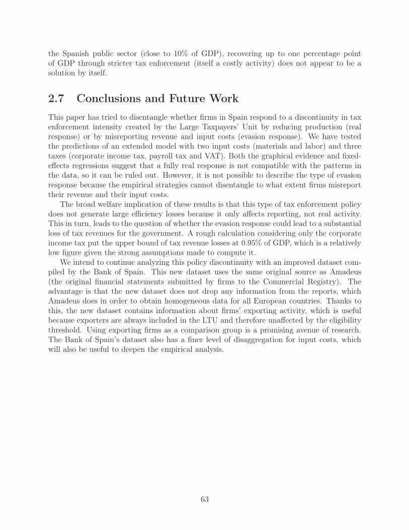
the Spanish public sector (close to 10% of GDP), recovering up to one percentage pointof GDP through stricter tax enforcement (itself a costly activity) does not appear to be asolution by itself.

2.7 Conclusions and Future Work

This paper has tried to disentangle whether firms in Spain respond to a discontinuity in taxenforcement intensity created by the Large Taxpayers’ Unit by reducing production (realresponse) or by misreporting revenue and input costs (evasion response). We have testedthe predictions of an extended model with two input costs (materials and labor) and threetaxes (corporate income tax, payroll tax and VAT). Both the graphical evidence and fixed-effects regressions suggest that a fully real response is not compatible with the patterns inthe data, so it can be ruled out. However, it is not possible to describe the type of evasionresponse because the empirical strategies cannot disentangle to what extent firms misreporttheir revenue and their input costs.

The broad welfare implication of these results is that this type of tax enforcement policydoes not generate large efficiency losses because it only affects reporting, not real activity.This in turn, leads to the question of whether the evasion response could lead to a substantialloss of tax revenues for the government. A rough calculation considering only the corporateincome tax put the upper bound of tax revenue losses at 0.95% of GDP, which is a relativelylow figure given the strong assumptions made to compute it.

We intend to continue analyzing this policy discontinuity with an improved dataset com-piled by the Bank of Spain. This new dataset uses the same original source as Amadeus(the original financial statements submitted by firms to the Commercial Registry). Theadvantage is that the new dataset does not drop any information from the reports, whichAmadeus does in order to obtain homogeneous data for all European countries. Thanks tothis, the new dataset contains information about firms’ exporting activity, which is usefulbecause exporters are always included in the LTU and therefore unaffected by the eligibilitythreshold. Using exporting firms as a comparison group is a promising avenue of research.The Bank of Spain’s dataset also has a finer level of disaggregation for input costs, whichwill also be useful to deepen the empirical analysis.

63

Tables

Table 2.1: Overview of the Spanish Tax System

Top tax rate Share of tax revenue

Social Security Contributions (SSC) 38% 33%Individual Income Tax (IIT) 48% (46%) 22%Value-Added Tax (VAT) 16% 19%Corporate Income Tax (CIT) 35% (30%) 13%Other indirect taxes and fees - 13%

Federal Tax Revenue / GDP 30-37%

Sources: Instituto de Estudios Fiscales (IEF, 2011). The top marginal rate of the individual incometax was reduced to 46% 2005. The top marginal rate of the corporate income tax was reduced to32.5% in 2006 and 30% in 2007. The data on tax revenues reflects averages for the period 1999-2007and include regional-level revenues in all calculations.

64

Tab

le2.

2:A

llIn

put

Cos

ts.

Fix

ed-E

ffec

tsR

egre

ssio

ns,19

99-2

011

All

Input

Cos

ts(%

ofR

even

ue)

,ye

arτ

All

Input

Cos

ts(%

ofR

even

ue)

,ye

arτ+

1(1

)(2

)(3

)(4

)(5

)(6

)(7

)(8

)

Bel

owT

hre

shol

d-0

.354

***

0.18

1*0.

288*

0.02

0( y i

τ≤

yLTU)

(0.1

46)

(0.0

94)

(0.1

20)

(0.0

61)

Low

Enfo

rcem

ent

0.11

70.

210*

**-0

.217

-0.1

30( y i

t≤

yLTU∀t≤

τ)

(0.1

21)

(0.0

80)

(0.1

34)

(0.1

03)

Con

stan

t92

.082

***

92.3

22**

*92

.280

***

89.9

31**

*92

.800

***

93.4

00**

*93

.139

***

89.8

00**

*(0

.148

)(0

.101

)(0

.098

)(0

.090

)(0

.004

)(0

.133

)(0

.111

)(0

.114

)

Firm

Fix

edE

ffec

tsno

yes

no

yes

no

yes

no

yes

Yea

rFix

edE

ffec

tsye

sye

sye

sye

sye

sye

sye

sye

sQ

uad

ratic

inR

even

ue

yes

yes

yes

yes

yes

yes

yes

yes

Obse

rvat

ions

263,

953

263,

953

263,

953

263,

953

263,

953

263,

953

263,

953

263,

953

Clu

ster

s64

,994

64,9

9464

,994

64,9

9464

,994

64,9

9464

,994

64,9

94R

-squ

ared

0.00

0.80

0.00

0.81

0.00

0.74

0.01

0.74

Not

e:Sta

ndar

der

rors

are

clust

ered

atth

efirm

leve

l.Sig

nifi

cance

leve

ls:

***

=1%

,**

=5%

,an

d*

=10

%.

The

sam

ple

isre

strict

edto

firm

sth

atre

por

ted

reve

nues

bet

wee

n€

3-€

9m

illion

atle

ast

one

year

inth

eper

iod

1999

-201

1.In

colu

mns

(1),

(2),

(5),

and

(6),

we

estim

ate

the

follow

ing

mod

el:

z it=

α+

φi+

λt+

ρ·f

( y it−

yLTU) +

β·

[ y iτ≤

yLTU] +

ε it,

wher

ez itis

tota

lre

por

ted

inputs

asa

per

cent

age

ofto

talre

venu

efo

rfirm

iin

year

t=

{τ,τ

+1}

,φiden

otes

firm

fixe

d-e

ffec

ts,λtden

otes

year

fixe

d-e

ffec

ts,f( y i

t−

yLTU)

isa

quad

ratic

pol

ynom

ialin

the

dis

tance

ofre

por

ted

reve

nue

toth

eth

resh

old,an

d[ y i

τ≤

yLTU]

isan

indic

ator

for

whet

her

firm

i’s

reve

nue

isbel

owth

eLT

Uth

resh

old

inye

arτ.

Inco

lum

ns

(3),

(4),

(7)

and

(8),

we

estim

ate

the

mod

el:

z it=

α+

φi+

λt+

ρ·f

( y it−yL

TU) +

β·

[ y it≤

yLTU∀t≤

τ] +

ε it,

wher

eth

ein

dic

ator

[ y it≤

yLTU∀t≤

τ]

take

sva

lue

one

for

firm

sth

ateff

ective

lyex

per

ience

low

enfo

rcem

ent,

i.e.

,firm

sw

hos

ere

por

ted

reve

nue

has

nev

erbee

nab

ove

the

LTU

thre

shol

d.

65

Tab

le2.

3:M

ater

ialIn

put

Cos

ts.

Fix

ed-E

ffec

tsR

egre

ssio

ns,19

99-2

011

Mat

eria

lIn

put

Cos

ts(%

ofR

even

ue)

,ye

arτ

Mat

eria

lIn

put

Cos

ts(%

ofR

even

ue)

,ye

arτ+

1(1

)(2

)(3

)(4

)(5

)(6

)(7

)(8

)

Bel

owT

hre

shol

d1.

675*

**0.

059

1.22

9***

-0.2

13( y i

τ≤

yLTU)

(0.3

39)

(0.1

14)

(0.3

50)

(0.1

52)

Low

Enfo

rcem

ent

1.67

9***

0.72

0***

0.69

3**

0.37

2***

( y it≤

yLTU∀t≤

τ)

(0.3

12)

(0.1

04)

(0.3

17)

(0.1

30)

Con

stan

t66

.502

***

67.6

58**

*66

.723

***

66.9

85**

*65

.658

***

64.8

13**

*66

.122

***

64.4

01**

*(0

.341

)(0

.128

)(0

.258

)(0

.115

)(0

.349

)(0

.164

)(0

.261

)(0

.139

)

Firm

Fix

edE

ffec

tsno

yes

no

yes

no

yes

no

yes

Yea

rFix

edE

ffec

tsye

sye

sye

sye

sye

sye

sye

sye

sQ

uad

ratic

inR

even

ue

yes

yes

yes

yes

yes

yes

yes

yes

Obse

rvat

ions

312,

481

312,

481

312,

481

312,

481

312,

481

312,

481

312,

481

312,

481

Clu

ster

s75

,694

75,6

9475

,694

75,6

9475

,694

75,6

9475

,694

75,6

94R

-squ

ared

0.01

0.94

0.01

0.94

0.01

0.91

0.01

0.91

Not

e:Sta

ndar

der

rors

are

clust

ered

atth

efirm

leve

l.Sig

nifi

cance

leve

ls:

***

=1%

,**

=5%

,an

d*

=10

%.

The

sam

ple

isre

strict

edto

firm

sth

atre

por

ted

reve

nues

bet

wee

n€

3-€

9m

illion

atle

ast

one

year

inth

eper

iod

1999

-201

1.In

colu

mns

(1),

(2),

(5),

and

(6),

we

estim

ate

the

follow

ing

mod

el:

z it=

α+

φi+

λt+

ρ·f

( y it−

yLTU) +

β·

[ y iτ≤

yLTU] +

ε it,

wher

ez itis

mat

eria

lin

put

cost

sas

aper

cent

age

ofto

talre

venu

efo

rfirm

iin

year

t=

{τ,τ

+1}

,φiden

otes

firm

fixe

d-e

ffec

ts,λtden

otes

year

fixe

d-e

ffec

ts,f( y i

t−

yLTU)

isa

quad

ratic

pol

ynom

ialin

the

dis

tance

ofre

por

ted

reve

nue

toth

eth

resh

old,an

d[ y i

τ≤

yLTU]

isan

indic

ator

for

whet

her

firm

i’s

reve

nue

isbel

owth

eLT

Uth

resh

old

inye

arτ.

Inco

lum

ns

(3),

(4),

(7)

and

(8),

we

estim

ate

the

mod

el:

z it=

α+

φi+

λt+

ρ·f

( y it−yL

TU) +

β·

[ y it≤

yLTU∀t≤

τ] +

ε it,

wher

eth

ein

dic

ator

[ y it≤

yLTU∀t≤

τ]

take

sva

lue

one

for

firm

sth

ateff

ective

lyex

per

ience

low

enfo

rcem

ent,

i.e.

,firm

sw

hos

ere

por

ted

reve

nue

has

nev

erbee

nab

ove

the

LTU

thre

shol

d.

66

Tab

le2.

4:Lab

orIn

put

Cos

ts.

Fix

ed-E

ffec

tsR

egre

ssio

ns,19

99-2

011

Lab

orIn

put

Cos

ts(%

ofR

even

ue)

,ye

arτ

Lab

orIn

put

Cos

ts(%

ofR

even

ue)

,ye

arτ+

1(1

)(2

)(3

)(4

)(5

)(6

)(7

)(8

)

Bel

owT

hre

shol

d-0

.682

***

0.04

0-0

.557

**0.

026

( y iτ≤

yLTU)

(0.2

08)

(0.0

60)

(0.2

18)

(0.0

98)

Low

Enfo

rcem

ent

-1.2

98**

*-0

.491

***

-1.1

29**

*-0

.804

***

( y it≤

yLTU∀t≤

τ)

(0.1

94)

(0.0

58)

(0.2

02)

(0.0

84)

Con

stan

t18

.842

***

12.3

51**

*18

.999

***

13.0

54**

*20

.065

***

14.5

67**

*20

.306

***

15.7

07**

*(0

.209

)(0

.074

)(0

.148

)(0

.070

)(0

.219

)(0

.112

)(0

.156

)(0

.095

)

Firm

Fix

edE

ffec

tsno

yes

no

yes

no

yes

no

yes

Yea

rFix

edE

ffec

tsye

sye

sye

sye

sye

sye

sye

sye

sQ

uad

ratic

inR

even

ue

yes

yes

yes

yes

yes

yes

yes

yes

Obse

rvat

ions

316,

924

316,

924

316,

924

316,

924

316,

924

316,

924

316,

924

316,

924

Clu

ster

s75

,730

75,7

3075

,730

75,7

3075

,730

75,7

3075

,730

75,7

30R

-squ

ared

0.01

0.96

0.01

0.96

0.02

0.90

0.02

0.90

Not

e:Sta

ndar

der

rors

are

clust

ered

atth

efirm

leve

l.Sig

nifi

cance

leve

ls:

***

=1%

,**

=5%

,an

d*

=10

%.

The

sam

ple

isre

strict

edto

firm

sth

atre

por

ted

reve

nues

bet

wee

n€

3-€

9m

illion

atle

ast

one

year

inth

eper

iod

1999

-201

1.In

colu

mns

(1),

(2),

(5),

and

(6),

we

estim

ate

the

follow

ing

mod

el:

z it=

α+

φi+

λt+

ρ·f

( y it−

yLTU) +

β·

[ y iτ≤

yLTU] +

ε it,

wher

ez it

isla

bor

input

cost

sas

aper

cent

age

ofto

talre

venu

efo

rfirm

iin

year

t=

{τ,τ

+1}

,φi

den

otes

firm

fixe

d-e

ffec

ts,λt

den

otes

year

fixe

d-e

ffec

ts,f( y i

t−

yLTU)

isa

quad

ratic

pol

ynom

ialin

the

dis

tance

ofre

por

ted

reve

nue

toth

eth

resh

old,an

d[ y i

τ≤

yLTU]

isan

indic

ator

for

whet

her

firm

i’s

reve

nue

isbel

owth

eLT

Uth

resh

old

inye

arτ.

Inco

lum

ns

(3),

(4),

(7)

and

(8),

we

estim

ate

the

mod

el:

z it=

α+

φi+

λt+

ρ·f

( y it−yL

TU) +

β·

[ y it≤

yLTU∀t≤

τ] +

ε it,

wher

eth

ein

dic

ator

[ y it≤

yLTU∀t≤

τ]

take

sva

lue

one

for

firm

sth

ateff

ective

lyex

per

ience

low

enfo

rcem

ent,

i.e.

,firm

sw

hos

ere

por

ted

reve

nue

has

nev

erbee

nab

ove

the

LTU

thre

shol

d.

67

Tab

le2.

5:N

umber

ofE

mpl

oyee

s.Fix

ed-E

ffec

tsR

egre

ssio

ns,19

99-2

011

Num

ber

ofE

mplo

yees

,ye

arτ

Num

ber

ofE

mplo

yees

,ye

arτ+

1(1

)(2

)(3

)(4

)(5

)(6

)(7

)(8

)

Bel

owT

hre

shol

d-1

.427

***

-0.3

94**

-1.5

33**

*-0

.501

**( y i

τ≤

yLTU)

(0.4

95)

(0.1

98)

(0.5

06)

(0.2

26)

Low

Enfo

rcem

ent

-1.7

55**

*-1

.423

***

-0.7

01-0

.742

***

( y it≤

yLTU∀t≤

τ)

(0.4

45)

(0.1

85)

(0.4

47)

(0.2

08)

Con

stan

t37

.739

***

34.8

61**

*37

.653

***

36.0

39**

*39

.168

***

35.6

69**

*38

.441

***

36.0

02**

*(0

.517

)(0

.242

)(0

.391

)(0

.216

)(0

.532

)(0

.263

)(0

.399

)(0

.231

)

Firm

Fix

edE

ffec

tsno

yes

no

yes

no

yes

no

yes

Yea

rFix

edE

ffec

tsye

sye

sye

sye

sye

sye

sye

sye

sQ

uad

ratic

inR

even

ue

yes

yes

yes

yes

yes

yes

yes

yes

Obse

rvat

ions

271,

704

271,

704

271,

704

271,

704

271,

704

271,

704

271,

704

271,

704

Clu

ster

s71

,227

71,2

2771

,227

71,2

2771

,227

71,2

2771

,227

71,2

27R

-squ

ared

0.05

0.92

0.05

0.93

0.05

0.91

0.05

0.91

Not

e:Sta

ndar

der

rors

are

clust

ered

atth

efirm

leve

l.Sig

nifi

cance

leve

ls:

***

=1%

,**

=5%

,an

d*

=10

%.

Inco

lum

ns

(1),

(2),

(5),

and

(6),

we

estim

ate

the

follow

ing

mod

el:

z it=

α+

φi+

λt+

ρ·f

( y it−

yLTU) +

β·

[ y iτ≤

yLTU] +

ε it,

wher

ez it

isth

enu

mber

ofem

plo

yees

infirm

iin

year

t=

{τ,τ

+1}

,φi

den

otes

firm

fixe

d-e

ffec

ts,λt

den

otes

year

fixe

d-e

ffec

ts,

f( y i

t−yL

TU)

isa

quad

ratic

pol

ynom

ial

inth

edis

tance

ofre

por

ted

reve

nue

toth

eth

resh

old,

and

[ y iτ≤

yLTU]

isan

indic

ator

for

whet

her

firm

i’s

reve

nue

isbel

owth

eLT

Uth

resh

old

inye

arτ.

Inco

lum

ns

(3),

(4),

(7)

and

(8),

we

estim

ate

the

mod

el:

z it=

α+

φi+

λt+

ρ·f

( y it−yL

TU) +

β·

[ y it≤

yLTU∀t≤

τ] +

ε it,

wher

eth

ein

dic

ator

[ y it≤

yLTU∀t≤

τ]

take

sva

lue

one

for

firm

sth

ateff

ective

lyex

per

ience

low

enfo

rcem

ent,

i.e.

,firm

sw

hos

ere

por

ted

reve

nue

has

nev

erbee

nab

ove

the

LTU

thre

shol

d.

68

Tab

le2.

6:Ave

rage

Wag

es.

Fix

ed-E

ffec

tsR

egre

ssio

ns,19

99-2

011

Ave

rage

Wag

es(t

hou

sands

ofeu

ros)

,ye

arτ

Ave

rage

Wag

es(t

hou

sands

ofeu

ros)

,ye

arτ+

1(1

)(2

)(3

)(4

)(5

)(6

)(7

)(8

)

Bel

owT

hre

shol

d-0

.841

***

-0.1

46-0

.829

***

-0.1

73( y i

τ≤

yLTU)

(0.2

34)

(0.1

65)

(0.2

44)

(0.1

76)

Low

Enfo

rcem

ent

-1.9

44**

*-0

.256

-2.1

15**

*-0

.287

*( y i

t≤

yLTU∀t≤

τ)

(0.2

06)

(0.1

65)

(0.2

11)

(0.1

67)

Con

stan

t26

.656

***

23.9

31**

*27

.435

***

24.3

17**

*27

.774

***

24.7

49**

*28

.651

***

25.0

82**

*(0

.225

)(0

.183

)(0

.156

)(0

.166

)(0

.231

)(0

.193

)(0

.159

)(0

.169

)

Firm

Fix

edE

ffec

tsno

yes

no

yes

no

yes

no

yes

Yea

rFix

edE

ffec

tsye

sye

sye

sye

sye

sye

sye

sye

sQ

uad

ratic

inR

even

ue

yes

yes

yes

yes

yes

yes

yes

yes

Obse

rvat

ions

268,

885

268,

885

268,

885

268,

885

268,

885

268,

885

268,

885

268,

885

Clu

ster

s70

,398

70,3

9870

,398

70,3

9870

,398

70,3

9870

,398

70,3

98R

-squ

ared

0.04

0.78

0.05

0.78

0.04

0.77

0.04

0.77

Not

e:Sta

ndar

der

rors

are

clust

ered

atth

efirm

leve

l.Sig

nifi

cance

leve

ls:

***

=1%

,**

=5%

,an

d*

=10

%.

Inco

lum

ns

(1),

(2),

(5),

and

(6),

we

estim

ate

the

follow

ing

mod

el:

z it=

α+

φi+

λt+

ρ·f

( y it−

yLTU) +

β·

[ y iτ≤

yLTU] +

ε it,

wher

ez it

isav

erag

ew

ages

(in

thou

sands

ofeu

ros)

infirm

iin

year

t=

{τ,τ

+1}

,φi

den

otes

firm

fixe

d-e

ffec

ts,λt

den

otes

year

fixe

d-

effec

ts,f( y i

t−

yLTU)

isa

quad

ratic

pol

ynom

ialin

the

dis

tance

ofre

por

ted

reve

nue

toth

eth

resh

old,an

d[ y i

τ≤

yLTU]

isan

indic

ator

for

whet

her

firm

i’s

reve

nue

isbel

owth

eLT

Uth

resh

old

inye

arτ.

Inco

lum

ns

(3),

(4),

(7)

and

(8),

we

estim

ate

the

mod

el:

z it=

α+

φi+

λt+

ρ·f

( y it−yL

TU) +

β·

[ y it≤

yLTU∀t≤

τ] +

ε it,

wher

eth

ein

dic

ator

[ y it≤

yLTU∀t≤

τ]

take

sva

lue

one

for

firm

sth

ateff

ective

lyex

per

ience

low

enfo

rcem

ent,

i.e.

,firm

sw

hos

ere

por

ted

reve

nue

has

nev

erbee

nab

ove

the

LTU

thre

shol

d.

69

Table 2.7: Lost Tax Revenue Calculations

Amadeus No frictions Frictions

Revenue Measure: As reported Reported + 1.4% Reported + 7.5%

Observations 553,956 553,956 553,956% with Positive Profits 64.8% 75.1% 83.4%Average Tax Liability (million €) 0.014 0.017 0.030Total Tax Liability (million €) 7,988.5 9,508.5 16,578.9Difference (million €) – 1,520.0 8,590.4Difference (% of tax revenue) – 0.48% 2.65%Difference (% of GDP) – 0.17% 0.95%

Note: this table summarizes the calculations of lost tax revenue in the low enforcement regimefor the year 2005. The first column shows the actual observations from Amadeus. The next twocolumns present the results of creating a new reported revenue measure equal to actual reportedrevenue plus a percentage based on the bunching estimates: 1.4% (no frictions estimate), and 7.5%(frictions estimate).

70

Figures

Figure 2.1: Reported Input Costs

Boom Period, 1999-2007

Reported Input Costs, Year t Reported Input Costs, Year t+1

88.0

90.0

92.0

94.0

96.0

98.0

Med

ian

of A

ll In

put C

osts

(% o

f Rev

enue

)

3 4 5 6 7 8 9Revenue (million Euros)

88.0

90.0

92.0

94.0

96.0

98.0

Med

ian

of A

ll In

put C

osts

(% o

f Rev

enue

), Ye

ar t+

1

3 4 5 6 7 8 9Revenue (million Euros)

Recession Period, 2008-2011

Reported Input Costs, Year t Reported Input Costs, Year t+1

88.0

90.0

92.0

94.0

96.0

98.0

Med

ian

of A

ll In

put C

osts

(% o

f Rev

enue

)

3 4 5 6 7 8 9Revenue (million Euros)

88.0

90.0

92.0

94.0

96.0

98.0

Med

ian

of A

ll In

put C

osts

(% o

f Rev

enue

), Ye

ar t+

1

3 4 5 6 7 8 9Revenue (million Euros)

Note: these graphs show the patterns of the ratio of reported input costs over revenue for the period1999-2007 (top panels) and 2008-2011 (bottom panels). Data are divided in €250,000 bins suchthat no bin includes firms both to the left and to the right of the LTU threshold, which is markedby the dashed (red) vertical line. The dots depict bin medians. The solid curves represent quadraticpolynomial fits estimated separately on each side of the threshold, and the dashed curves are 95%confidence intervals.

71

Figure 2.2: Material Input Costs

Boom Period, 1999-2007

Material Input Costs, Year t Material Input Costs, Year t+1

62.0

64.0

66.0

68.0

70.0

72.0

Med

ian

of M

ater

ial I

nput

Cos

ts (%

of R

even

ue)

3 4 5 6 7 8 9Revenue (million Euros)

62.0

64.0

66.0

68.0

70.0

72.0

Med

ian

of M

ater

ial I

nput

Cos

ts (%

of R

ev.),

Yea

r t+1

3 4 5 6 7 8 9Revenue (million Euros)

Recession Period, 2008-2011

Material Input Costs, Year t Material Input Costs, Year t+1

5860

6264

6668

Med

ian

of M

ater

ial I

nput

Cos

ts (%

of R

even

ue)

3 4 5 6 7 8 9Revenue (million Euros)

5860

6264

6668

Med

ian

of M

ater

ial I

nput

Cos

ts (%

of R

ev.),

Yea

r t+1

3 4 5 6 7 8 9Revenue (million Euros)

Note: these graphs show the patterns of the ratio of material input costs over revenue for the period1999-2007 (top panels) and 2008-2011 (bottom panels). Data are divided in €250,000 bins suchthat no bin includes firms both to the left and to the right of the LTU threshold, which is markedby the dashed (red) vertical line. The dots depict bin medians. The solid curves represent quadraticpolynomial fits estimated separately on each side of the threshold, and the dashed curves are 95%confidence intervals.

72

Figure 2.3: Labor Input Costs

Boom Period, 1999-2007

Labor Input Costs, Year t Labor Input Costs, Year t+1

10.0

12.0

14.0

16.0

18.0

20.0

Med

ian

of L

abor

Cos

ts (%

of R

even

ue)

3 4 5 6 7 8 9Revenue (million Euros)

10.0

12.0

14.0

16.0

18.0

20.0

Med

ian

of L

abor

Cos

ts (%

of R

ev.),

Yea

r t+1

3 4 5 6 7 8 9Revenue (million Euros)

Recession Period, 2008-2011

Labor Input Costs, Year t Labor Input Costs, Year t+1

10.0

12.0

14.0

16.0

18.0

20.0

Med

ian

of L

abor

Cos

ts (%

of R

ev.),

Yea

r t+1

3 4 5 6 7 8 9Revenue (million Euros)

12.0

14.0

16.0

18.0

20.0

22.0

Med

ian

of L

abor

Cos

ts (%

of R

ev.),

Yea

r t+1

3 4 5 6 7 8 9Revenue (million Euros)

Note: these graphs show the patterns of the ratio of labor input costs over revenue for the period1999-2007 (top panels) and 2008-2011 (bottom panels). Data are divided in €250,000 bins suchthat no bin includes firms both to the left and to the right of the LTU threshold, which is markedby the dashed (red) vertical line. The dots depict bin medians. The solid curves represent quadraticpolynomial fits estimated separately on each side of the threshold, and the dashed curves are 95%confidence intervals.

73

Figure 2.4: Average Wages

Boom Period, 1999-2007

Average Wages, Year t Average Wages, Year t+1

23.0

25.0

27.0

29.0

31.0

Med

ian

of A

vera

ge G

ross

Wag

e (’0

00s

Euro

s)

4 5 6 7 8Revenue (million Euros)

23.0

25.0

27.0

29.0

31.0

Med

ian

of A

vera

ge G

ross

Wag

e (’0

00s

euro

s), Y

ear t

+1

4 5 6 7 8Revenue (million Euros)

Recession Period, 2008-2011

Average Wages, Year t Average Wages, Year t+1

29.0

31.0

33.0

35.0

37.0

Med

ian

of A

vera

ge G

ross

Wag

e (’0

00s

Euro

s)

4 5 6 7 8Revenue (million Euros)

29.0

31.0

33.0

35.0

37.0

Med

ian

of A

vera

ge G

ross

Wag

e (’0

00s

euro

s), Y

ear t

+1

4 5 6 7 8Revenue (million Euros)

Note: these graphs show the patterns of average wages (in thousands of euros) for the period 1999-2007 (top panels) and 2008-2011 (bottom panels). Data are divided in €250,000 bins such thatno bin includes firms both to the left and to the right of the LTU threshold, which is marked bythe dashed (red) vertical line. The dots depict bin medians. The solid curves represent quadraticpolynomial fits estimated separately on each side of the threshold, and the dashed curves are 95%confidence intervals.

74

Figure 2.5: Number of Employees

Boom Period, 1999-2007

Number of Employees, Year t Number of Employees, Year t+1

2025

3035

4045

Med

ian

of N

umbe

r of E

mpl

oyee

s

4 5 6 7 8Revenue (million Euros)

2025

3035

4045

Med

ian

of N

umbe

r of E

mpl

oyee

s, Y

ear t

+1

4 5 6 7 8Revenue (million Euros)

Recession Period, 2008-2011

Number of Employees, Year t Number of Employees, Year t+1

2025

3035

4045

Med

ian

of N

umbe

r of E

mpl

oyee

s

4 5 6 7 8Revenue (million Euros)

2025

3035

4045

Med

ian

of N

umbe

r of E

mpl

oyee

s, Y

ear t

+1

4 5 6 7 8Revenue (million Euros)

Note: these graphs show the patterns of the number of employees for the period 1999-2007 (toppanels) and 2008-2011 (bottom panels). Data are divided in €250,000 bins such that no bin includesfirms both to the left and to the right of the LTU threshold, which is marked by the dashed (red)vertical line. The dots depict bin medians. The solid curves represent quadratic polynomial fitsestimated separately on each side of the threshold, and the dashed curves are 95% confidenceintervals.

75

Chapter 3

Firm Size Responses to Labor Regulations: Evidence

from France

3.1 Introduction

Size-contingent labor regulations are ubiquitous in many countries. The goal of such regu-lations is often to give small firms more labor market flexibility and increase their growthpotential. However, the existence of regulatory thresholds dampens the incentives to grow,potentially defeating the purpose of these policies (Heckman and Pages, 2003). Understand-ing the impact of this type of regulations on employment and firm growth is important toinform the design of labor market policies.

In this paper, I study the impact of a regulatory threshold in France, where there are34 different labor laws that apply only to firms with 50 or more employees. One of theselaws requires firms to create a comité d’entreprise (works council) that empowers unionswithin the firm; another imposes bureaucratic limits to worker separations, and a third oneestablishes of a profit-sharing scheme by which employees receive a share of annual profits.1

Overall, these regulations increase the average labor cost per employee for French businessesby about 4% (according to Attali, 2008) and give firms a strong incentive to remain belowthe 50-employee threshold.

In the absence regulatory thresholds, we would expect the firm size distribution, measuredby the number of employees, to be smoothly decreasing as in other developed economies (see,for example, Braguinsky, Branstetter and Regateiro, 2011). Using data from Amadeus forthe period 2002-2008, I document that a nontrivial group of firms strategically choose to“bunch” below the threshold in order to avoid the additional regulations. The bunchingpattern is stable when analyzing each annual sample separately, so I rely on the pooleddataset to obtain more precise estimates. In terms of growth patterns, I show that theproportion of firms increasing their size from one year to the next drops almost by half at 49employees (35% vs. 20%), while the share of firms keeping a constant number of employeesdoubles at 49 employees (15 vs. 30%).

The structural parameter of interest in this context is the elasticity of labor demand

1Ceci-Renaud and Chevalier (2010) and the online appendix of Garicano, LeLarge and van Reenen (2013)provide detailed descriptions of all the relevant regulations.

76

implied by the response to the regulatory threshold. Departing from the traditional laboreconomics approach surveyed by Hamermesh (1986, 1993), I apply techniques from a recentliterature in public finance that uses discontinuities in tax systems to estimate income taxelasticities (Saez, 2010; Chetty et al., 2011; Kleven and Waseem, 2013).2 To estimate theelasticity of labor demand, I first set up a stylized model with labor as the only factor ofproduction and a discontinuity in average labor costs at an employment cutoff. In thismodel, firms receive an exogenous productivity draw (as in Lucas, 1978) that determinestheir optimal size. The model predicts the existence of three types of firms in equilibrium:(i) low-productivity firms that are too small to be affected by regulations, (ii) bunchingfirms that cut back their number of employees to be exactly at the cutoff, and (iii) high-productivity firms that reduce their number of employees due to the regulations, but notenough to avoid them.

I derive an expression for the elasticity of labor demand that can be estimated using thenumber of bunching firms as a sufficient statistic.3 The key to the estimation strategy is toconstruct a counterfactual firm size distribution and then estimate the number of bunchingfirms as the difference between the observed distribution and the counterfactual in an intervalbelow the cutoff. Applying this method, I obtain a point estimate of eNF = 0.055 for theelasticity of labor demand pooling data from the period 2002-2008, which is statisticallydifferent from zero at the 10% level. Making an adjustment for the possibility that some firmsdo not respond to the regulations due to optimization frictions, I obtain a point estimateof eF = 0.572, which can be interpreted as an upper bound for the long-term structuralelasticity, although it is imprecisely estimated (the standard error is 0.668).

These point estimates are considerably below labor demand elasticities estimated in theliterature, which according to Hamermesh (1993) tend to be in the interval (0.15, 0.75). Anintuitive explanation for why I obtain such a low point estimate is that bunching firms maybe adjusting their production by increasing the use of other inputs instead of labor. I findsome preliminary evidence supporting this hypothesis: median fixed assets per employeedrop sharply at the notch, indicating that bunching firms have a higher capital-labor ratiothan firms just above the threshold. This implies that the model should incorporate otherproduction inputs such as capital, and the estimation strategy should consider the elasticityof substitution between capital and labor. This is left for future work.

The study of French labor regulations and their influence on the firm size distributionis not new. Ceci-Renaud and Chevalier (2010) were the first to document the bunchingat the 50-employee regulatory threshold in a descriptive study where they also documentbunching at 10 and 20 employees.4 Garicano, LeLarge and van Reenen (2013) focus on theimpact of these regulations on the productivity of French firms. They structurally estimate

2Saez (2010) and Chetty et al. (2011) study “kinks” in the budget set, define as points where the marginaltax rate jumps discontinuously. Meanwhile, Kleven and Waseem (2013) study “notches”, defined as pointswhere both the marginal and the average tax rate jump. In the current paper, I study a notch in labor costs,because there is a discontinuous upward jump in labor costs at the 50-employee threshold. For a review ofthe relationship between the two concepts, see Slemrod (2010).

3Chetty (2009b) summarizes the general characteristics of this approach, which he argues is a bridgebetween reduced-form and structural estimation methods.

4Schivardi and Torrini (2008) provide similar evidence for Italy, where key employment protection legis-lation applies only to firms with more than 15 employees.

77

a model based on Lucas (1978) and calculate that the welfare loss associated with labormarket regulations is 0.8% of GDP assuming flexible wages and up to 5.1% of GDP whenassuming wage rigidities. The key contribution of the current paper is to provide an estimatefor the labor demand elasticity using an alternative empirical approach to the same setting.Knowledge about this structural parameter can be useful to understand firm behavior inresponse to other shock and also inform new labor market policies.

This paper is also related to a literature that shows how micro-level distortions canaffect aggregate productivity through resource misallocation. Guner, Ventura and Xu (2008)calibrate a growth model with endogenous size distribution of establishments. They findthat size-dependent policies can generate substantial reductions in output by increasingthe equilibrium number of establishments but reducing output per establishment.5 Hsiehand Klenow (2009) show that resource misallocation accounts for a significant share of thedifferences in aggregate productivity between China, India and the US.

The remainder of the paper is organized as follows. Section 2 presents the theoreticalframework and derives an estimation strategy for the labor demand elasticity. Section 3provides background on French labor regulations and describes the data. Section 4 reportsthe graphical evidence and the elasticity estimations. Section 5 discusses the welfare impli-cations. Section 6 concludes.

3.2 Theoretical Framework and Empirical Strategy

3.2.1 Setup

Consider an economy with a finite number of firms and no entry or exit. Each firm has amanagerial productivity θi with p.d.f. g (θ), and a production function where labor (l) is theonly factor of production, where F ′ (l) > 0 and F ′′ (l) < 0.6 Labor is infinitely elasticallysupplied at wage rate w. All non-wage labor costs stemming from labor regulations arecombined into a single parameter, ϕ, that I will refer to as a “labor tax”. Notice that ϕ isexpressed as a percentage of net wages received by workers, w. Let C (l,ϕ, w) denote thecost function faced by the firm, which I assume to be linear: C (l,ϕ, w) = (1 + ϕ)wl.

In the standard version of the model, labor costs are the same for all firms, ϕi = ϕ0 ∀i.Firms maximize the following profit function:

max{li} πi = θiF (li)−(1 + ϕ0

)wli (3.1)

The first order condition for an interior solution is

li(θi,ϕ

0)= F ′−1

((1 + ϕ0)w

θi

), (3.2)

which defines optimal labor demand for firm i. Since we have assumed that θi ∼ g (θ), thereexists some h (·) such that li (θi,ϕ) ∼ h (l), where the shape of h (·) depends on g (·) and

5In a closely related paper, Restuccia and Rogerson (2008) build a growth model with heterogeneousestablishments to show that policy distortions (defined in a general way that includes size-dependent policies)that apply only to some of them make the most efficient ones produce too little and employ too few workers.

6The basic setup of this model follows the seminal contribution of Lucas (1978) to the literature of firmsize distributions, although that model does not incorporate taxes.

78

the specific production function. If the p.d.f. of the managerial productivity distribution issmooth, the distribution of firm size will also be smooth.

3.2.2 Introducing a Small Notch

The government introduces a new set of labor regulations that increase the labor tax fromϕ0 to ϕ1 > ϕ0. These regulations only apply to firms above a certain number of employeesl∗, that is:

ϕi =

{ϕ0 if li ≤ l∗

ϕ1 = ϕ0 +∆ϕ if li > l∗(3.3)

where ∆ϕ > 0 is assumed to be small. From the point of view of the firm, the new regulationsincrease the average cost per employee, including those that already worked for the firm(i.e., all inframarginal employees). Hence, this changes introduces a notch in the labor costfunction at l∗ employees. A notch is defined as a point in the budget set where both theaverage and the marginal tax rate jump. It is different from a kink, which is a point wherethe marginal tax rate jumps but the average tax rate varies smoothly.

Figure 3.1 depicts the incentives created by the notch. The straight lines from the originrepresent labor cost functions under the two labor taxes, ϕ0 and ϕ1. After the reform,firms face the labor cost function represented by the solid sections of these lines, with adiscontinuous upward jump at the notch. The graph shows isoprofit curves for two firms,A and B, with managerial productivity levels θA and θB > θA. Firm A maximizes profitschoosing lA = l∗ under the initial labor tax rate and also under the higher rate. In contrast,Firm B chooses lB (ϕ0) > l∗ under the low labor tax but is indifferent between choosing l∗

and l∗ + dl∗ employees once the notch is introduced. I assume, without loss of generality,that firm B chooses lB (ϕ1) = l∗. It follows that every firm i with managerial productivityθi ∈ (θA, θB) also chooses li = l∗.

The consequences of this analysis for the firm size distribution (measured by the numberof employees) can be seen in Figure 3.2, which depicts the theoretical firm size distribution(measured by number of employees). The counterfactual density distribution is depicted bythe black dashed curve, which is smoothly decreasing by the assumptions on the distributionof managerial productivity. The observed distribution, depicted in the red solid curve, depictswhat happens once the notch is introduced. There are three types of firms in the newequilibrium with the notch: low productivity firms, bunching firms, and high productivityfirms. Low productivity firms have θi ∈ [θmin, θ∗) and they choose li < l∗ under both taxregimes.7 Bunching firms have productivities in the range θi ∈ [θ∗, θ∗ + dθ∗), and they allchoose li = l∗ in response to the reform, “bunching” at the notch.8 I define firm B as themarginal buncher, i.e. the firm with the highest managerial productivity level that choosesli = l∗. Finally, high productivity firms have θi ∈ [θ∗ + dθ∗, θmax) and they choose li > l∗

both with and without the notch. These firms reduce their demand for employment afterthe notch is introduced, but they do not bunch at the notch because it is too costly for themto reduce their scale that much.

7For completeness, firms with θi < θmin never enter the market, because their optimal labor demand isnegative so they cannot produce anything.

8Notice that θA = θ∗ and θB = θ∗ + dθ∗.

79

3.2.3 Derivation of the Elasticity of Labor Demand

In order to derive an expression for the elasticity of labor demand in this model, I start bydefining gross wages paid by the firm as wg ≡ (1 + ϕ)w. Then, I write the elasticity of labordemand with respect to the average labor cost as:

eALC = −∆l/l

∆wg/wg= −

∆l/l

∆ϕ/ (1 + ϕ)(3.4)

This elasticity captures the percentage response of labor demand to a one percent change inlabor costs. While this magnitude might be of interest in some particular cases, economicmodels usually define elasticities with respect to marginal changes in the price, because theygive more general information.

The technical problem is that the labor cost functions has a discontinuity at the notch,so its derivative (the marginal cost of labor) is not defined at l = l∗. I approximate the“effective” marginal labor cost following the methodology proposed by Kleven and Waseem(2013). The idea is to consider what is the change in the marginal labor cost faced by themarginal buncher, relating the change in the tax rate, ∆ϕ, with the change in labor demand,∆l, as follows:

ϕe =C (l∗ +∆l∗)− C (l∗)

∆l∗* ϕ0 +

∆ϕ

∆l∗l∗ (3.5)

This is depicted by the red dashed line in Figure 3.1, which links the two indifference pointsfor firm B and has a slope equal to (1 + ϕe)w. An intuitive interpretation of 80 is that thecost of an additional unit of labor for firm B is the original marginal cost ϕ0 plus the extralabor cost ∆ϕ that now has to be paid for all the existing employees (l∗). The latter termis averaged over the actual increase in employees, ∆l∗. The size of this second term dependsnot only on the magnitude of the change in the labor cost, but also on the shape of theproduction function and the resulting isoprofit curves.

Given the above expression for ϕe, the elasticity of labor demand with respect to themarginal labor cost, evaluated at employment level l∗, can be written as:

eMLC = −∆l∗/l∗

∆ϕe/ (1 + ϕe)* −

(∆l∗/l∗)2

∆ϕ/ (1 + ϕ)(3.6)

Notice that, in the final expression of eMLC , the denominator is again the average cost oflabor, while the numerator is squared.

3.2.4 Elasticity Estimation

Recall that, in equilibrium, li ∼ h (l). The small notch generated by an increase of ∆ϕ inthe labor tax leads a group of firms to bunch. The marginal buncher now chooses to hirel∗ employees, but it used to choose lMB

(θMB,ϕ0

)= l∗ + ∆l∗, where ∆l∗ is related to dϕ

through the shape of the density function g (θ). The term ∆l∗ is the length of the intervalwhere no firms locate in Figure (3.2). Then, let the number of bunching firms be defined as

B =

ˆ l∗+∆l∗

l∗h (l) dl ≈ h (l∗)∆l∗, (3.7)

80

where the approximation relies on ∆ϕ > 0 being small. Substituting (3.7) into (3.6), Iobtain:

eMLC = −(B/ [h (l∗) l∗])2

∆ϕ/ (1 + ϕ)(3.8)

All the terms in expression (3.8) are either parameters or can be estimated empirically.The parameters are the value of the notch, l∗ = 50 in this setting, and the change in the taxrate, ∆ϕ/ (1 + ϕ). To estimate the number of bunching firms, B, I construct a counterfactualdensity distribution that in turn provides the value of h (l∗). Hence, the number of bunchingfirms is a sufficient statistic to estimate the elasticity of labor demand.

In order to construct the counterfactual density, I follow the standard methods from thebunching literature (e.g., Saez, 2010; Chetty et al., 2011; Kleven and Waseem, 2013). I firstrun a polynomial fit of the count of firms at each employee level (that is, the height of thebars in the histogram) on the number of employees:

Si =p∑

j=1

βj (li − l∗)j +lub∑

j=llb

γ0j · 1 {li = j}+ ε0i (3.9)

where Si is the number of firms with exactly i employees, (li − l∗) is the distance of i fromthe threshold (so the notch is at 0), p is the order of the polynomial and llb and lub are thelower and upper bound of the excluded interval where the counterfactual diverges from theactual density. The counterfactual density is obtained by taking predicted values from theestimates of (3.9), excluding the γk shifters:

Si =p∑

j=0

βj · (li − l∗)j (3.10)

Comparing this counterfactual density to the observed distribution allows us to estimatethe excess bunching mass to the left of the threshold (B), and similarly the missing mass tothe right of the threshold (H):

B =l∗∑

l=llb

∣∣∣Sj − Sj

∣∣∣ H =lub∑

l=l∗

∣∣∣Sj − Sj

∣∣∣ (3.11)

Determining the lower and upper bounds of the excluded region in a consistent wayis critical for this estimation method to provide credible estimates. I follow the approachof Kleven and Waseem (2013), which is based on the principle that the area under thecounterfactual density has to equal the area under the observed density. I start by settingan arbitrary lower bound, llb, and then run equation (3.9) multiple times. Regarding theupper bound, in the first iteration I set lub ≈ l∗, which tends to yield large estimates of Band small estimates of H . The estimation routine is programmed to increase the value oflub by one employee and run equation (3.9) again as long as B > H. The process continuesuntil it reaches a value of lub such that B = H . This procedure provides an estimate of thenumber of bunching (and missing) firms following the formulas in (3.11).

Since this estimation procedure is applied to the universe of French firms rather thana random sample, there is no sampling error and therefore I cannot construct the usual

81

confidence intervals around the estimates of B and H . To generate standard errors, I samplethe residuals from regression (3.9) a large number of times (with replacement) to obtainbootstrapped standard errors. Finally, I apply the delta method to calculate standard errorsaround the elasticity estimates.

Optimization Frictions

Contrary to the prediction of the stylized model (pictured in Figure 3.2), there may be no“hole” in the firm size distribution above the notch. This would suggest that some firms arenot able to adjust their number of employees as easily as others, and end up just above thecutoff despite the additional costs.

Optimization frictions have been a widely discussed issue in the bunching literature, asdescribed in Chapter 1. The number of employees differs from reported revenue on severalcharacteristics. First, it is a discrete variable, rather than continuous. Second, it is a stockinstead of a flow. This matters dynamically because hiring a new worker today might havean impact in next year’s number of employees, which is not the case for revenue. Moregenerally, labor market rigidities make hiring and firing decisions less reversible than theywould be in a frictionless world. Given all these reasons, it is important to allowing for thepossibility that some firms may not be able to respond to the notch’s incentives even thoughit would be optimal for them to do so.

Other sources of optimization frictions might come from searching and training coststhat prevent firms from growing or laying off workers. Moreover, there might be uncertaintyabout the future so that there is a “region of inaction” in which firms do not adjust theirfactor demands in response to small shocks, as argued by Bloom (2009). In this particularcontext, a plausible hypothesis is that, once a firm has already been subject to the additionalregulations, it cannot revert to the old situation by simply firing some employees and goingback below the cutoff. For example, the committees that are created when crossing the50-employee mark cannot be dissolved without approval from the unions. Thus, having beenabove the threshold in previous years could be a good predictor of locating in the intervaljust above 50 employees.

I incorporate the possibility of optimization frictions into the elasticity estimation follow-ing the approach proposed by Kleven and Waseem (2013). I define α as the proportion offirms locating in the interval (l∗, lub], compared to the counterfactual density. I use this mea-sure to re-weight the estimates so that BF = B

1−α , where the subscript F indicates that the

new estimator accounts for optimization frictions. Then, I introduce BF into the elasticityformula:

eF = −(BF/ [h (l∗) l∗])

2

∆ϕ/ (1 + ϕ)(3.12)

The estimates of eF can be interpreted as an upper bound of the structural elasticity pa-rameter.

82

3.3 Institutional Context and Data

3.3.1 Labor Regulations in France

There are at least 34 different labor regulations in France that only apply to firms with morethan 50 employees (Attali, 2008). Some other regulations apply only to firms above 10 or 20employees. Comprehensive summaries of all these regulations are presented in Ceci-Renaudand Chevalier (2010) and in the online appendix of Garicano, LeLarge and van Reenen(2013). In this paper, I focus on the 50-employee threshold, which is the most important interms of the difference in average labor costs on each side of the cutoff. I summarize belowthe key regulations that apply above this threshold.

Firms with more than 50 employees have to set up a Works Council (“comité d’entreprise”),which meets bi-monthly to discuss workplace issues. This committee is comprised of 3-4 rep-resentatives of the employees, usually appointed by the unions, who get 20 paid hours permonth to perform committee duties. Firms also have to set up committees on hygiene andsafety of working conditions. Additionally, they have to establish a profit-sharing scheme, bywhich employees receive a pre-determined share of annual profits (which varies by sector).Another law regulates collective dismissals, defined as the separation of 9 or more employeesin any given month. A firm that wants to carry out a collective dismissal needs to design a“social plan”, monitored by the Ministry of Labor and negotiated with the unions, in orderto facilitate re-employment of laid-off workers. There is evidence that this process usuallytakes up substantial administrative resources from firms.

It is hard to provide a precise measure of the costs that these regulations impose onfirms, in part because there is probably a great deal of heterogeneity. In order to obtainelasticity estimates using the methodology outlined above, it is necessary to assign a specificlabor tax rate to this package of regulations. A reasonable source for this estimate is Attali(2008), a report commissioned by the French government to implement an ambitious reformprogram. Attali (2008) estimates, based on a large survey of firm managers, that the packageof regulations that kicks in at 50 employees implies an extra labor cost equivalent to 4% ofthe total wage bill for the average firm in the 50-250 employees range.

3.3.2 Data

I use data from Amadeus, a comprehensive database of European businesses put togetherby Bureau van Dijk, a market research company (www.bvdinfo.com), already described inChapter 1. The dataset covers annual accounting reports from French firms for the period2002-2009. The information available for each firm in each year includes: business name,location (5-digit postal code), sector of activity at the 4-digit level, 26 balance sheet items,26 profit and loss account items, and 32 standard financial ratios.

Table 3.1 reports the number of firms reporting their number of employees in each yearduring this period. The number of firms grows from just above 300,000 in 2002 to 900,000in 2008 and almost 1.8 million in 2009. Part of the trend is probably due to actual growthin business registration, but the bulk of the change is due to other factors. First, the onlineversion of Amadeus accessed for this paper (through Wharton Research Data Services) onlymaintains firms in the dataset for 4 years after their last report. Thus, if a firm disappeared

83

in 2008, it would not be in the dataset in 2013. Second, in some cases Amadeus doesnot digitalize the entire financial statements when firms submit them in paper form, butthis is not an issue when the submission is electronic. A change in the proportion of firmssubmitting electronically is likely to explain the doubling in the number of firms from 2008to 2009. As can be seen in Table 3.1, most of the increase in 2009 is due to firms with 10or fewer employees. In any case, to avoid any sample selection issues, when I pool data forseveral years in the empirical analysis I use the period 2002-2008.

3.4 Results

3.4.1 Graphical Evidence

I begin by studying the cross-sectional distribution of firm size, measured by the numberof employees. In the absence of size-contingent labor regulations, the firm size distribution(FSD) should follow a smoothly declining distribution, approximately lognormal (Cabral andMata, 2003). Hence, any deviations of the FSD from a smooth counterfactual distributioncan be attributed to the existence of the regulatory cutoff.

Figure 3.3 shows the firm size distribution around the 50-employee threshold using pooleddata from the years 2002-2008. Pooling increases sample size and it is consistent with theinstitutional context because the same set of labor regulations was applicable throughout theperiod. The year-by-year distributions look very similar, as shown in Figure 3.7. There is alarge spike in the density starting at 49 employees, and then a drop from 50 onwards.9 Thenumber of firms with 49 employees more than doubles the number of firms with 50 employees.The bunching response indicates a behavioral response to labor regulations, as predicted bythe theoretical framework. Moreover, the lack of a “hole” in the density above the notchsuggests that there are non-negligible optimization frictions that prevent some firms fromadjusting. In the next subsection, I quantify the bunching response and provide estimates forthe implied elasticity of labor demand both under the assumptions of optimization frictionsand the stylized frictionless model. Figure 3.4 shows the firm size distribution around thetwo other regulation thresholds at 10 and 20 employees. There seems to be bunching in bothcases, although the jump in the density at the notch is proportionally smaller.

The two graphs in Figure 3.5 describe the dynamics of firm growth in France. The toppanel plots the proportion of firms that grow in the following year (vertical axis) againsttheir current size (horizontal axis), defining growth as having more employees in year t + 1than in year t. The proportion increases with the number of employees, but it drops sharplybelow each of the three regulatory thresholds. In particular, the proportion of growingbusinesses drops from 35% for 40-employee firms to 20% for 49-employee firms. The dashedlines indicate 95% confidence intervals for each bin, which indicate that the downward jumpis statistically significant. In the bottom panel, the y-axis variable is the proportion of firmsthat keep the same number of employees in year t+1 as they had in year t. The proportiondecreases with firm size, but it jumps up from 15% for 40-employee firms to about 30% for

9It seems that the additional labor regulations applied to firms with “50 and more” employees for theperiod 2002-2008. The data for 2009 actually shows the largest spike at 50 employees. I am not certain ofwhether this is due to a change in one specific regulation or a larger subset.

84

49-employee firms (also statistically significant).To sum up, there is strong evidence that some firms strategically reduce their growth when

they reach 49 employees in order to avoid being subject by the additional labor regulations.

3.4.2 Elasticity Estimations

Using the method described in the empirical strategy section, I construct a counterfactualfirm size distribution, shown in Figure 3.6. The blue connected dots represent a histogramwith the same data as Figure 3.3. The orange dashed line depicts the counterfactual dis-tribution. The vertical dashed lines indicate the lower and upper bounds of the excludedregion, respectively. Based on visual observation, I pick llb = 40 and the estimation routinedetermines that lub = 63. The estimated number of bunching firms over the 9-year period isB = 8, 223, from a sample of 208, 058 firms between 20 and 80 employees. To approximatethe change in labor costs associated with the labor regulations, I use the estimates from theAttali (2008) report, such that ∆ϕ/ (1 + ϕ) = 4%.

Table 3.2 reports the elasticity estimates for the pooled 2002-2008 data and also for eachyear’s sample. The “no frictions” estimate for the pooled data is eNF = 0.055 with standarderror 0.032, so it is statistically significant at the 10% level. The point estimate allowingfor optimization frictions is eNF = 0.572 with std. error 0.668, which is not statisticallydistinguishable from zero (nor one). The point estimates are remarkably similar for all theyears between 2002 and 2009, with slightly larger variation on the standard errors. The “nofrictions” elasticity is marginally significant in three years, while the “frictions” elasticity isnot significant in any year.

In a thorough review on the topic, Hamermesh (1993) reviews the existing estimates ofthe labor demand elasticity from previous studies and concludes that the average is around0.3, with a confidence (0.15, 0.75). This puts the “no frictions” estimates below the lowerbound of the distribution, which is somewhat surprising considering the sharp bunchingobserved in the size distribution. The key to understanding this apparent contradiction isthat a notch creates very strong incentives, so with a labor demand elasticity of 0.3 we wouldhave observed much stronger bunching at 49 employees.

3.4.3 Other Margins of Adjustment

It is clear that the stylized one-input model that we have imposed on the data might bedriving these low estimates of the structural elasticity. A natural extension is to includeother production inputs in the model, such as capital or materials, and study the elasticityof substitution around the notch.

As a preliminary inquiry into this possible adjustment margins, Figure 3.8 plots thedistributions of fixed assets per employee (a proxy for the capital-labor ratio, k/l) andmaterial input expenses per employee. The graphs show median values for groups of firmswith the same number of employees for the pooled sample 2002-2008. The top panel of Figure3.8 shows that the median capital-labor ratio increases with the number of employees, butthere is a sharp drop exactly at the notch, going from a median of €15,000 in fixed assets peremployee for 49-employee firms to a median of €12,000 for 50-employee firms. In the bottom

85

panel, there is also a small break in the pattern of median material inputs per employee atthe notch, but it is less clear that the overall trends differ on either side of the threshold.

The positive correlation between fixed assets and material expenditures and locatingjust below the regulatory threshold suggests that bunching firms may be substituting awayfrom labor and into other inputs as they approach the cutoff. In future work, I plan toderive the model with multiple production inputs and a constant elasticity of substitution(CES) technology. Hamermesh (1993) shows how to bring this model to the data in order toestimate both the labor demand elasticity and the elasticity of substitution between laborand other inputs. The latter elasticity is interesting in its own right, and it will also allowme to disentangle to what extent those margins of adjustment bias my estimates of the labordemand elasticity towards zero.

3.5 Welfare Implications

Using the estimates for the elasticity of labor demand from the previous section, I can makean estimation of the deadweight loss (DWL) associated with the additional labor marketregulations. In particular, I attempt to estimate the welfare loss due to the fact that, inresponse to the higher labor costs, some firms reduce their demand for labor but workers donot fully capture the surplus lost by firms.

Recall that firms in the model are heterogeneous in their managerial productivity θ, sothe standard DWL formulas for a representative agent cannot be applied. I then calculatethe individual DWL for a each firm and then aggregate over all firms. Given that the modelassumes an infinitely elastic labor supply curve, the DWL is simply the area below eachfirm’s demand curve and above the market wage, over the interval (li (θi,ϕ0) , li (θi,ϕ1)):

DWLi *(ϕ1 + ϕ0)w

2[−∆li]

*(ϕ1 + ϕ0)w

2

[−e

∆ϕ

(1 + ϕ)li (θi)

](3.13)

When aggregating for the entire economy, I do not include low productivity firms becausethey are not affected by the new regulations. The impact on bunching firms is larger than onhigh-productivity firms because they change their labor demand more, but the same formulaapplies to all firms with productivity in the range θ ∈ [θ∗, θmax). Then, aggregate DWL isgiven by:

DWL =

ˆ θmax

θ∗

(ϕ1 + ϕ0)w

2

[−e

∆ϕ

(1 + ϕ)l (θ)

]dθ (3.14)

This calculation yields an aggregate deadweight loss 0.42% of the total wage bill, whenthe “no frictions” elasticity estimation is considered, and of 1.78% when the upper boundestimate (allowing for frictions).

In a study that analyzes the same set of labor regulations, Garicano et al. (2013) struc-turally estimate a model based on Lucas (1978). They calculate that the welfare loss associ-ated with the French labor market regulations is 0.8% of GDP when assuming flexible wagesand up to 5.1% of GDP when assuming wage rigidities. In the flexible wage case (similar to

86

the assumptions made in this paper), the output loss is small and the drop in efficiency comesalmost entirely from the tax aspect of regulations. (Garicano et al., 2013) point out that thetax could be considerecd a transfer to workers, but they provide suggestive evidence showingthat workers do not place high value on the amenities obtained from more union power andnew committees. In the rigid wage model, the regulations lead to higher unemployment andthus lower substantially lower output, which accounts for most of the efficiency loss in thatcase.

3.6 Conclusion and Future Work

I have studied the impact of labor regulation thresholds on the production behavior of Frenchfirms. About 34 different labor regulations apply only to firms with 50 or more employees,giving firms an incentive to bunch just below this threshold. Using a stylized model with onlyone factor of production, I have derived an elasticity of labor demand that can be estimateddirectly using the number of bunching firms as a sufficient statistic.

I obtain a point estimate of eNF = 0.055 for the elasticity of labor demand in Francein the period 2002-2008, which is statistically different from zero at the 10% level. Makingan adjustment for the possibility that some firms do not respond to the regulations due tooptimization frictions, I obtain a point estimate of eF = 0.572, which could be interpreted asan upper bound for the long-term structural elasticity, although it is imprecisely estimated(the standard error is 0.668).

These point estimates are considerably below other labor demand elasticities estimated inthe literature, which according to Hamermesh (1993) tend to be in the interval (0.15, 0.75).An intuitive explanation for these low estimates is that bunching firms might be adjustingtheir production by increasing the use of other inputs instead of labor. As an example, Ihave shown that median fixed assets per employee are much higher for bunching firms thanfor firms immediately above the threshold.

The next step in this research project is to explore potential extensions to the modelto make it more realistic and allow a better identification of the structural elasticities. Oneextension discussed in the main text is to consider multiple inputs in the production function,and study the elasticity of substitution between labor and other inputs. Another possibleextension is to endogenize wage determination by allowing the labor supply curve to beupward sloping. In a model with endogenously determined wages, firms above the thresholdwould pay lower wages to their employees in equilibrium, because the regulations act asa benefit that the employees receive(Summers, 1989). A countervailing effect is that, onaverage, larger firms tend to pay higher wages. This relationship is likely to be monotonicover firm size, while the “benefit” effect would create a jump at the threshold. Finding a wayto test this hypothesis using the incentives created by the regulatory cutoff seems to be apromising avenue for future research.

A more ambitious extension of the model would be to add dynamics and uncertainty.This would allow me to incorporate the possibility of good versus bad economic conditions,which complicates the hiring and firing decisions of the firm as expectations come into play.In this dynamic model, firm owners would need to trade-off present versus future benefitsand costs.

87

Tables

Table 3.1: Amadeus Data, French Firms

0-10 Employees 11-100 Employees 100+ Employees Total

2002 260,084 38,559 6,572 305,2152003 449,474 61,639 8,450 519,5632004 506,774 68,298 8,920 583,9922005 566,252 70,202 9,141 645,5952006 646,454 62,486 8,925 717,8652007 739,836 61,299 9,109 801,2442008 827,869 58,484 8,408 894,7612009 1,702,772 67,455 8,606 1,778,833

Note: this table shows the evolution of the sample size in the Amadeus dataset for French firms.Only firms with a nonmissing value for the number of employees are counted. A change in theproportion of firms submitting electronically is likely to explain the doubling in the number of firmsfrom 2008 to 2009. As can be seen in the table, most of the increase in 2009 is due to firms with 10or fewer employees. To avoid any sample selection issues, when I pool data for several years in theempirical analysis I always use the period 2002-2008.

88

Table 3.2: Labor Demand Elasticity Estimates

eNF eF B H llb lub NPooled Data

2002-2008 0.055* 0.572 8,223.5 8,530.1 40 63 208,058(0.032) (0.668)

Annual Data

2002 0.050 0.564 784.1 900.1 40 64 20,439(0.040) (3.759)

2003 0.065* 0.565 1,289.3 1,363.2 40 63 30,801(0.037) (0.622)

2004 0.057* 0.506 1,318.3 1,257.0 40 61 33,480(0.031) (0.516)

2005 0.055 0.508 1,323.0 1,421.5 40 63 33,921(0.045) (0.995)

2006 0.062* 0.744 1,282.4 1,304.0 40 65 30,690(0.034) (1.737)

2007 0.041 0.424 1,066.0 1,293.8 40 63 30,318(0.027) (0.534)

2008 0.056 0.677 1,140.2 1,094.5 40 63 28,409(0.043) (3.066)

Note: eNF and eF are the labor demand elasticities assuming no frictions and frictions, respectively.B is the number of firms above the counterfactual density in the range l ∈ (llb, l∗), where l is numberof employees, llb is the lower bound of the excluded region (used to construct the counterfactual)and l∗ is the regulatory threshold of 50 employees. H is the missing number of firms below thecounterfactual density in the range l ∈ (l∗, lub), where lub is the upper bound of the excluded region.Finally, N is the number of observations included in the estimations, i.e. the number of firms withl ∈ (20, 80) in each year. Significance levels: *** = 1%, ** = 5%, and * = 10%.

89

Figures

Figure 3.1: Discontinuity in Labor Costs

!" !"#$!" !"#$%&''(

!"#$%&'!

!"#$"%&'!

()!*+,-$.%

(/!*+#0*+,-$.%

(/!*+#0*+,-$"%

123456-!"#$5%&'!

7!!"#$!"%

7!!"%

)*+%,-.%(/(

Note: this diagram shows equilibrium in a model with a notch in labor costs at l∗ employees. Thevertical axis shows total labor costs: wage (w) times employees (l) multiplied by one plus the tax onlabor (1+ϕ). The horizontal axis plots the number of employees. The rays from the origin depicttotal labor costs under low and high tax rates, ϕ0 and ϕ1. The higher tax only applies to firms withmore than l∗ employees, so the schedule of labor costs is determined by the solid black lines, witha discontinuous upward jump at l∗. The curves represent isoprofit curves for firm A and B, whichhave managerial productivity levels θA = θ∗ and θB = θ∗ + dθ∗, respectively.

90

Figure 3.2: Theoretical Employees Distribution with a Notch

!" !"#$!"

!"#$%&'()$"*+",-,"#$%&'

./0#&"*123&024-,"#$%&'

50#36%#7-8*9$-:5;

<%$$%#7-92$$-:=;

>9?4/'""$

Note: this figure depicts the theoretical revenue distribution before and after the introduction oflabor regulations. In the standard scenario, the distribution of number of employees is smoothlydecreasing, as depicted by the dashed (black) line. When additional labor regulations are introduced,firms with more than l∗ employees face higher average labor costs. A group of firms in an intervalabove l∗ respond to the new regulations by reducing their size to have exactly l∗ employees. Thisgenerates a spike at the threshold (with excess mass B), and an area of missing mass (H) to theright of the threshold, as depicted by the solid (red) line. Notice that this plot assumes that thereare no optimization frictions, so all firms can immediately respond to fiscal incentives. Thus, thereare no firms in the interval of length ∆l∗ above the threshold.

91

Figure 3.3: Firm Size Distribution

0.0

1.0

2.0

3.0

4.0

5D

ensi

ty

20 30 40 50 60 70 80Number of Employees

N=208058

Years 2002−2008

Note: this histogram shows the distribution of firm size in France, measured by the number ofemployees. The vertical red line indicates that firms above that size (50 employees) are subject toa set of 34 labor regulations. The graph pools data for the period 2002-2008, throughout whichthe regulations were applicable. Bin width is one, meaning that the histograms show the raw datawithout any adjustments.

92

Figure 3.4: Bunching at Other Thresholds0

.05

.1.1

5.2

Den

sity

0 2 4 6 8 10 12 14 16 18 20Number of Employees

N=1273227

Years 2002−2008

0.0

5.1

.15

Den

sity

10 12 14 16 18 20 22 24 26 28 30Number of Employees

N=305373

Years 2002−2008

Note: these two histograms show the distribution of firm size in France, measured by the number ofemployees. The vertical dashed lines indicate that firms with more than 10 employees (left) or 20employees (right) are subject to additional labor regulations. The graphs pool data for the period2002-2008, throughout which the regulations were applicable. Bin width is one, meaning that thehistograms show the raw data without any adjustments.

93

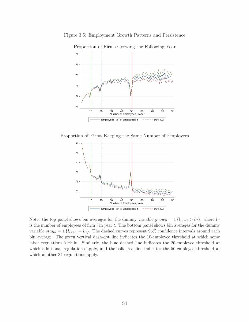
Figure 3.5: Employment Growth Patterns and Persistence

Proportion of Firms Growing the Following Year

.1.2

.3.4

.5.6

10 20 30 40 50 60 70 80 90Number of Employees, Year t

Employees_t+1 > Employees_t 95% C.I.

Proportion of Firms Keeping the Same Number of Employees

.1.2

.3.4

.5.6

10 20 30 40 50 60 70 80 90Number of Employees, Year t

Employees_t+1 = Employees_t 95% C.I.

Note: the top panel shows bin averages for the dummy variable growit = 1 {li,t+1 > lit}, where litis the number of employees of firm i in year t. The bottom panel shows bin averages for the dummyvariable stayit = 1 {li,t+1 = lit}. The dashed curves represent 95% confidence intervals around eachbin average. The green vertical dash-dot line indicates the 10-employee threshold at which somelabor regulations kick in. Similarly, the blue dashed line indicates the 20-employee threshold atwhich additional regulations apply, and the solid red line indicates the 50-employee threshold atwhich another 34 regulations apply.

94

Figure 3.6: Counterfactual Firm Size Distribution, 2002-2008

Years 2002-2008

020

0040

0060

0080

0010

000

Num

ber o

f Firm

s

20 30 40 50 60 70 80Number of Employees

Actual Density Counterfactual DensityN=208058

Note: the dots connected by a solid blue line represent a histogram of the number of employees,using exactly the same data as Figure 3.3. The orange dashed line shows the counterfactual firmsize distribution. The vertical dotted blue lines indicate the lower and upper bounds of the excludedregion, llb and lub. To determine these values, I first fix the value of llb = 40 employees and then fita polynomial fit to the density, starting with lub ≈ l∗ = 50. I then increase the value of lub in unitsteps until the are between the observed density and the counterfactual in the range (llb, 50) equalsthe are between the two densities in the range (50, lub).

95

Fig

ure

3.7:

Cou

nter

fact

ualFir

mSi

zeD

istr

ibut

ion,

Yea

rby

Yea

r

2002

2003

2004

02004006008001000Number of Firms

2030

4050

6070

80N

umbe

r of E

mpl

oyee

s

Actu

al D

ensi

tyC

ount

erfa

ctua

l Den

sity

N=2

0439

050010001500Number of Firms

2030

4050

6070

80N

umbe

r of E

mpl

oyee

s

Actu

al D

ensi

tyC

ount

erfa

ctua

l Den

sity

N=3

0801

050010001500Number of Firms

2030

4050

6070

80N

umbe

r of E

mpl

oyee

s

Actu

al D

ensi

tyC

ount

erfa

ctua

l Den

sity

N=3

3480

2005

2006

2007

050010001500Number of Firms

2030

4050

6070

80N

umbe

r of E

mpl

oyee

s

Actu

al D

ensi

tyC

ount

erfa

ctua

l Den

sity

N=3

3921

050010001500Number of Firms

2030

4050

6070

80N

umbe

r of E

mpl

oyee

s

Actu

al D

ensi

tyC

ount

erfa

ctua

l Den

sity

N=3

0690

050010001500Number of Firms

2030

4050

6070

80N

umbe

r of E

mpl

oyee

s

Actu

al D

ensi

tyC

ount

erfa

ctua

l Den

sity

N=3

0318

2008

2009

20040060080010001200Number of Firms

2030

4050

6070

80N

umbe

r of E

mpl

oyee

s

Actu

al D

ensi

tyC

ount

erfa

ctua

l Den

sity

N=2

8409

050010001500Number of Firms

2030

4050

6070

80N

umbe

r of E

mpl

oyee

s

Actu

al D

ensi

tyC

ount

erfa

ctua

l Den

sity

N=3

0741

Not

e:th

ese

annu

alplo

tsar

eco

nst

ruct

edin

the

sam

ew

ayas

Fig

ure

3.6.

96

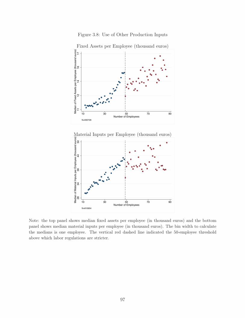
Figure 3.8: Use of Other Production Inputs

Fixed Assets per Employee (thousand euros)

1112

1416

17M

edia

n of

Fix

ed A

sset

s pe

r Em

ploy

ee (t

hous

and

euro

s)

10 30 50 70 90Number of Employees

N=930726

Material Inputs per Employee (thousand euros)

2834

3944

50M

edia

n of

Mat

eria

l Inp

uts

per E

mpl

oyee

(tho

usan

d eu

ros)

10 30 50 70 90Number of Employees

N=810654

Note: the top panel shows median fixed assets per employee (in thousand euros) and the bottompanel shows median material inputs per employee (in thousand euros). The bin width to calculatethe medians is one employee. The vertical red dashed line indicated the 50-employee thresholdabove which labor regulations are stricter.

97

Bibliography

AEAT, “Memoria de Administración Tributaria,” Technical Report, Agencia Estatal deAdministración Tributaria (Spanish Tax Agency) Several years.

Allingham, Michael and Agnar Sandmo, “Income tax evasion: A theoretical analysis,”Journal of Public Economics, 1972, 1, 323–338.

Andreoni, James, Brian Erard, and Jonathan Feinstein, “Tax Compliance,” Journalof Economic Literature, June 1998, 36, 818–860.

Attali, Jacques, “Rapport de la Commission pour la libération de la croissance française("Report for the Commission for the Liberation of French Growth"),” 2008. Report com-missioned by French President Nicolas Sarkozy.

Bastani, Spencer and Hakan Selin, “Bunching and Non-Bunching at Kink Points of theSwedish Tax Schedule,” June 2012. CESifo Working Paper No. 3865.

Bayer, Ralph and Frank Cowell, “Tax compliance and firms’ strategic interdependence,”Journal of Public Economics, 2009, 93, 1131–1143.

Bloom, Nicholas, “The impact of uncertainty shocks,” Econometrica, 2009, 77, 623–685.

BOE, “Ley de Presupuestos Generales del Estado,” Several years. Boletín Oficial del Estado.

Braguinsky, Serguey, Lee Branstetter, and Andre Regateiro, “The Incredible Shrink-ing Portuguese Firm,” July 2011. NBER Working Paper 17265.

Cabral, Luís and José Mata, “On the Evolution of the Firm Size Distribution: Facts andTheory,” American Economic Review, September 2003, 93 (4), 1075–1090.

Ceci-Renaud, Nila and Paul-Antoine Chevalier, “L’impact del seuils de 10, 20 et 50salariés sur la taille des entreprises françaises,” Économie et Statistique, 2010, 437, 29–45.

Chetty, Raj, “Is the Taxable Income Elasticity a Sufficient Statistic to Calculate Dead-weight Loss? The Implications of Evasion and Avoidance,” American Economic Journal:Economic Policy, 2009, 1 (2), 31–52.

, “Sufficient Statistics for Welfare Analysis: A Bridge Between Structural and Reduced-Form Analysis,” Annual Review of Economics, June 2009, 1, 451–488.

98

, “Bounds on Elasticities with Optimization Frictions: A Synthesis of Micro and MacroEvidence on Labor Supply,” Econometrica, May 2012, 80 (3), 969–1018.

, John Friedman, and Emmanuel Saez, “Using Differences in Knowledge AcrossNeighborhoods to Uncover the Impacts of the EITC on Earnings,” July 2012. NBERWorking Paper 18232.

, , Tore Olsen, and Luigi Pistaferri, “Adjustment Costs, Firm Responses, andMicro vs. Macro Labor Supply Elasticities: Evidence from Danish Tax Records,” QuarterlyJournal of Economics, 2011, 126, 749–804.

Christensen, Kevin, Robert Cline, and Tom Neubig, “Total Corporate Taxation:"Hidden", Above-the-Line, Non-Income Taxes,” National Tax Journal, 2001, LIV (3),495–506.

Devereux, Michael, Li Liu, and Simon Loretz, “The Elasticity of Corporate TaxableIncome: New Evidence from UK Tax Records,” January 2013. Oxford University Centrefor Business Taxation Working Paper 12/23.

Dharmapala, Dhammika, Joel Slemrod, and John Douglas Wilson, “Tax policy andthe missing middle: Optimal tax remittance with firm-level administrative costs,” Journalof Public Economics, October 2011, 95 (9-10), 1036–1047.

Feldstein, Martin, “The Effect of Marginal Tax Rates on Taxable Income: A Panely Studyof the 1986 Tax Reform Act,” Journal of Political Economy, June 1995, 103 (3), 551–572.

, “Tax Avoidance and The Deadweight Loss of Income Taxation,” Review of Economicsand Statistics, November 1999, 81 (4), 674–680.

Garicano, Luis, Claire LeLarge, and John van Reenen, “Firm Size Distrotions andthe Productivity Distribution: Evidence from France,” February 2013. NBER WorkingPaper 18841.

Guner, Nezih, Gustavo Ventura, and Yi Xu, “Macroeconomic Implications of Size-Dependent Policies,” Review of Economic Dynamics, 2008, 11, 721–744.

Hamermesh, Daniel, “The demand for labor in the long run,” Handbook of Labor Eco-nomics, 1986, 1.

, The Demand for labor, Princeton, NJ: Princeton University Press, 1993.

Heckman, James and Carmen Pages, “Law and Employment: Lessons from Latin Amer-ica and the Caribbean,” December 2003. NBER Working Paper 10129.

Hsieh, Chang-Tai and Peter Klenow, “Misallocation and Manufacturing TFP in Chinaand India,” Quarterly Journal of Economics, November 2009, CXXIV (4), 1403–1448.

IEF, “Evolución del Sistema Fiscal Español: 1978-2010,” 2011. Instituto de Estudios Fiscales.

99

IMF, “Improving Large Taxpayers’ Compliance: A Review of Country Experience,” Techni-cal Report, International Monetary Fund, Washington DC 2002. Team led by KatherineBaer.

Kleven, Henrik and Mazhar Waseem, “Using Notches to Uncover Optimization Fric-tions and Structural Elasticities: Theory and Evidence from Pakistan,” forthcoming at theQuarterly Journal of Economics, 2013.

, Klaus Kreiner, and Emmanuel Saez, “Why Can Modern Governments Tax So Much?An Agency Model of Firms as Fiscal Intermediaries,” August 2009. NBER Working Paper15218.

Kumler, Todd, Eric Verhoogen, and Judith Frias, “Enlisting Workers in MonitoringFirms: Payroll Tax Compliance in Mexico,” June 2012.

LaCaixa, “Por Qué No Aumenta la Dimensión de la Empresa Española?,” May 2012. LaCaixa Research Department.

Lee, David and Thomas Lemieux, “Regression Discontinuity Designs in Economics,”Journal of Economic Literature, June 2010, 48, 281–355.

Lucas, Robert, “On the Size Distribution of Business Firms,” The Bell Journal of Eco-nomics, Autumn 1978, 9 (2), 508–523.

Marx, Benjamin, “Regulatory Hurdles and Growth of Charitable Contributions: Evidencefrom a Dynamic Bunching Design,” November 2012. Columbia University.

OECD, “Tax Administration in OECD and Selected non-OECD Countries: ComparativeInformation Series (2010),” Technical Report, Organisation for Economic Co-operationand Development March 2011.

Paula, Áureo De and José Scheinkman, “Value-Added Taxes, Chain Effects, and Infor-mality,” American Economic Journal: Macroeconomics, October 2010, 2, 195–221.

Pomeranz, Dina, “No Taxation Without Information: Deterrence and Self-Enforcement inthe Value-Added Tax,” April 2013. Harvard Business School Working Paper 13-057.

Reinganum, Jennifer and Louis Wilde, “Income Tax Compliance in a Principal-AgentFramework,” Journal of Public Economics, 1985, 26, 1–18.

Restuccia, Diego and Richard Rogerson, “Policy Distortions and Aggregate Productiv-ity with Heterogeneous Establishments,” Review of Economic Dynamics, 2008, 11, 707–720.

Saez, Emmanuel, “Do Taxpayers Bunch at Kink Points?,” American Economic Journal:Economic Policy, August 2010, 2 (3), 180–212.

Schivardi, Fabiano and Roberto Torrini, “ “Identifying the effects of firing restrictionsthrough size-contingent differences in regulation,” Labour Economics, 2008, 15, 482–511.

100

Schneider, Friedrich, Andreas Buehn, and Claudio Montenegro, “ShadowEconomies all over the World: New Estimates for 162 Countries from 1999 to 2007,”Working Paper 322, Universidad de Chile 2010.

Slemrod, Joel, “The economics of corporate tax selfishness,” National Tax Journal, De-cember 2004, LVII (4), 877–900.

, “Does it Matter Who Writes the Check to the Government? The Economics of TaxRemittance,” National Tax Journal, June 2008, LXI (2), 251–275.

, “Buenas Notches: Lines and Notches in Tax System Design,” 2010. Working Paper,University of Michigan.

Summers, Lawrence, “Simple Economics of Mandated Benefits,” American Economic Re-view, Papers and Proceedings, May 1989, 79 (2), 177–183.

101