Embed Size (px)
Citation preview

This PDF is a selection from an out-of-print volume from the National Bureauof Economic Research
Volume Title: Orders, Production, and Investment: A Cyclical and StructuralAnalysis
Volume Author/Editor: Victor Zarnowitz
Volume Publisher: NBER
Volume ISBN: 0-870-14215-1
Volume URL: http://www.nber.org/books/zarn73-1
Publication Date: 1973
Chapter Title: Size and Frequency of Fluctuations
Chapter Author: Victor Zarnowitz
Chapter URL: http://www.nber.org/chapters/c3550
Chapter pages in book: (p. 70 - 128)

3SIZE AND FREQUENCY OF
FLUCTUATIONS
THIS CHAPTER DEALS principally with the amplitude aspects of therelations between new orders, production, and shipments. It describesthe comprehensive series for the postwar period, in current and con-stant dollars, with the aid of charts and comparisons of relative cyclicalamplitudes. The analysis is then extended to data for individual in-dustries, for selected economic indicators, and for the interwar period.Measures based on statistical decomposition of the time series bytype of movement are used in this part of the chapter.
Postwar Cycles in Comprehensive Series
Current Data on New Orders and Shipments of Major IndustriesThe main body of data on the value of manufacturers' new orders
and shipments is the monthly compilation by the U.S. Department ofCommerce, which goes back to the Survey established in1939 by the Office of Business Economics (OBE). The OBE datacover the years after World War II and are given in changing pricesof the period; the over-all totals for the durable and nondurable goodssectors begin in 1939.
In 1957, the processing of the Industry Survey was transferredwithin the Commerce Department to the Bureau of the Census, whichpublished, in October 1963, a major revision of the survey series onmanufacturers' shipments, orders, and inventories.1 The new Census
Bureau of the Census, Manufacturers' Shipments, Inventories, and Orders: 194 7—1963 (Re-vised), Washington, D.C., 1963.

Size and Frequency of Fluctuations 71
data carry the totals for durable goods industries, nondurable goodsindustries, and all manufacturing, back to 1947; the series for compo-nent industries and the newly introduced market-grouped categories,back to 1953.
The revised data set differs from the old one in several respects:(1) The coverage of the survey has been broadened significantly,particularly with regard to large companies; (2) the sample design hasbeen revised as a probability sample to give better representation ofthe entire manufacturing universe; (3) improved industry reportingand new benchmark levels have permitted a reorientation from acompany base to a divisional or establishment base; (4) as a result, thenew survey is able to provide more detailed and homogeneous industryfigures as well as aggregates for market categories which cut across theindustry groups, separating materials from final products and, amongthe latter, consumer goods from industrial equipment, defense items,etc.2
Because of these differences in concept or estimation procedure, theold and new component series differ rather substantially, though pri-marily in level and much less in change characteristics such as ampli-tudes and timing. Before the 1963 revision was published, I had com-pleted an analysis of the earlier data, and the charts and tables that fol-low are based in part on that analysis. However, much of this work wasreplicated with the aid of the new series, to keep the study as up todate as possible and to incorporate the presumably improved statisticalinformation now available. A warning is due here that these latest dataare not strictly comparable with the earlier series used for the yearsbefore 1953, though care has been exercised to avoid any inferencesthat could be invalidated by such noncomparabilities. Only for the mostcomprehensive aggregates are the currently published series continu-ous over the entire postwar period.
In the Commerce data of all vintages, the comparability of the ordersand shipments figures is assured by the method of their estimation: thevalue of new orders in any month t is derived by adding to the value ofshipments in the same month the change, centered on t, in the esti-mated end-of-month totals of unfilled orders. This procedure is ap-
2 For a further discussion of these and some other features of the Commerce data and somecomparisons of the old and new series, see ibid.
72 Relationships Between New Orders, Production, and Shipments
plied to data before seasonal adjustment. The resulting figures are netof cancellations.3
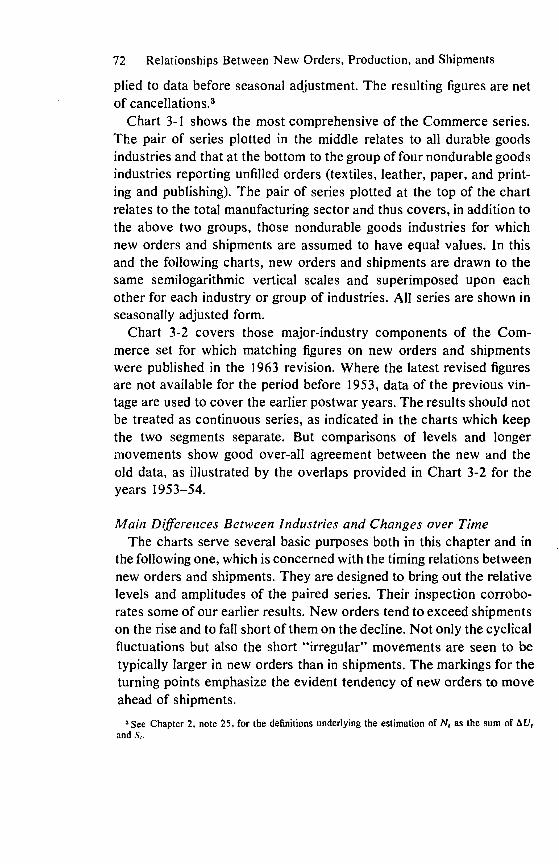
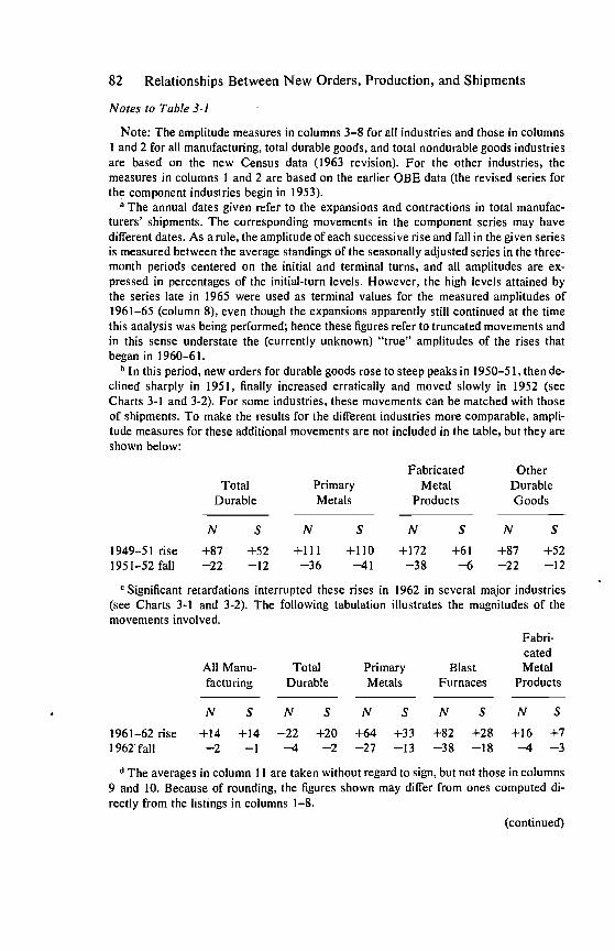
Chart 3-1 shows the most comprehensive of the Commerce series.The pair of series plotted in the middle relates to all durable goodsindustries and that at the bottom to the group of four nondurable goodsindustries reporting unfilled orders (textiles, leather, paper, and print-ing and publishing). The pair of series plotted at the top of the chartrelates to the total manufacturing sector and thus covers, in addition tothe above two groups, those nondurable goods industries for whichnew orders and shipments are assumed to have equal values. In thisand the following charts, new orders and shipments are drawn to thesame semilogarithmic vertical scales and superimposed upon eachother for each industry or group of industries. All series are shown inseasonally adjusted form.
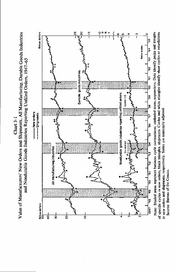
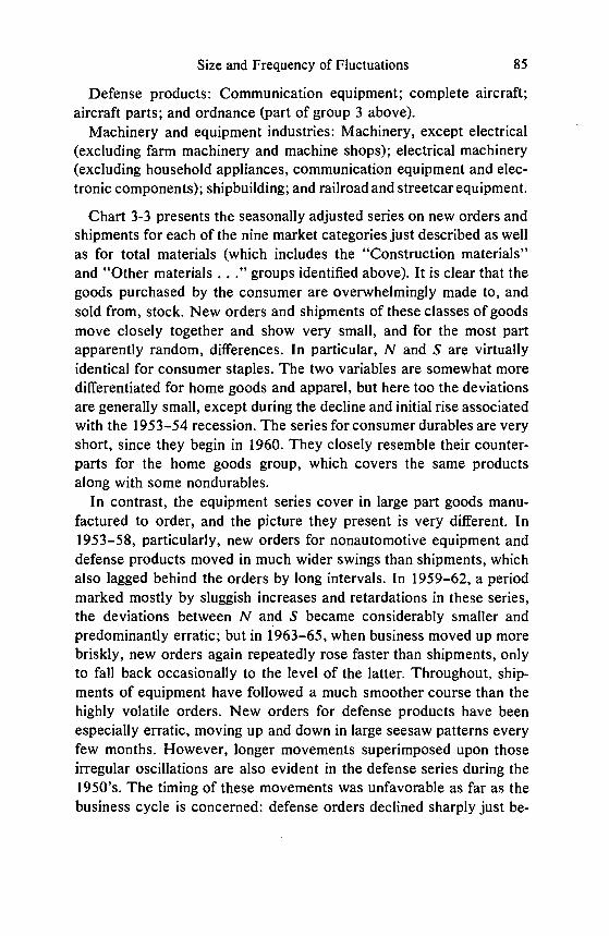
Chart 3-2 covers those major-industry components of the Com-merce set for which matching figures on new orders and shipmentswere published in the 1963 revision. Where the latest revised figuresare not available for the period before 1953, data of the previous vin-tage are used to cover the earlier postwar years. The results should notbe treated as continuous series, as indicated in the charts which keepthe two segments separate. But comparisons of levels and longermovements show good over-all agreement between the new and theold data, as illustrated by the overlaps provided in Chart 3-2 for theyears 1953—54.
Main Differences Between Industries and Changes over TimeThe charts serve several basic purposes both in this chapter and in
the following one, which is concerned with the timing relations betweennew orders and shipments. They are designed to bring out the relativelevels and amplitudes of the paired series. Their inspection corrobo-rates some of our earlier results. New orders tend to exceed shipmentson the rise and to fall short of them on the decline. Not only the cyclicalfluctuations but also the short "irregular" movements are seen to betypically larger in new orders than in shipments. The markings for theturning points emphasize the evident tendency of new orders to moveahead of shipments.
' See Chapter 2, note 25, for the definitions underlying the estimation of N1 as the sum ofand
Cha
rt 3
-1V
alue
of
Man
ufac
ture
rs' N
ew O
rder
s an
d Sh
ipm
ents
, All
Man
ufac
turi
ng, D
urab
le G
oods
Ind
ustr
ies
and
Non
dura
ble
Goo
ds I
ndus
trie
s R
epor
ting
Unf
illed
Ord
ers,
194
7—65
Not
e: S
hade
d ar
eas
repr
esen
t bus
ines
s cy
cle
cont
ract
ions
; uns
hade
d ar
eas,
exp
ansi
ons.
Dot
s id
entif
y pe
aks
and
trou
ghs
of s
peci
fic
cycl
es in
new
ord
ers;
bla
ck tr
iang
les,
shi
pmen
ts. C
ircl
es a
nd w
hite
tria
ngle
s id
entif
y sh
ort c
ycle
s or
ret
arda
tions
in n
ew o
rder
s an
d sh
ipm
ents
, res
pect
ivel
y. S
erie
s ar
e se
ason
ally
adj
uste
d.So
urce
: Bur
eau
of th
e C
ensu
s.
New
ord
ers
Shi
pmen
tsB
iIRO
n do
llars
Bill
ion
dolla
rs
'62
'63
'64

Chart 3-2Value of Manufacturers' NewOrders and Shipments, SevenMajor Durable Goods In-
dustries, 1948—65
Note: Shaded areas represent busi-ness cycle contractions; unshadedareas, expansions. Dots identify peaksand troughs of specific cycles in neworders; black triangles, shipments.Circles and white triangles identifyshort cycles or retardations in new or-ders and shipments, respectively.Series are seasonally adjusted.
Source: 1948—54: U.S. Departmentof Commerce, Office of Business Eco-nomics; 1953—65: Bureau of theCensus.
74
New orders
BflUon dol'arsShipments
New ordersShipments
75
Ratio scales
2.0
1.5
1.0
2.0
1.5
7
6
5
4
3
2

76 Relationships Between New Orders, Production, and Shipments
However, while these characteristics are general and often con-spicuous, the intensity and regularity with which they appear varygreatly for different industries and periods. First, there is the smoothingeffect of aggregation: the series that cover broad divisions of industryare in general less erratic than those relating to the more narrowlydefined components (compare, e.g., the over-all aggregates in Chart3-1 with the major-industry series in Chart 3-2, for new orders andshipments, separately). This, of course, is merely one manifestation ofthe familiar rule applicable to various types of economic process.
Second, new orders and shipments move much closer together inthe nondurable goods sector of manufacturing than in the durablegoods one. The nondurable aggregates in Chart 3-1 include only thoseindustries that report unfilled orders (textiles, leather, paper, and print-ing and publishing). The other components of the sector, with consider-ably larger values of production and sales, work predominantly to stockand for them new orders and shipments are assumed to be identical inthe Commerce statistics. Thus, had I plotted the all-inclusive series forthe nondurables, the differences between orders and shipments wouldhave appeared much smaller still. As it is, relatively large discrepanciesbetween the two series for the four-industry group reporting unfilledorders are observable only in the 1948—49 recession and during theKorean War period in 1950—51; for the new set of data beginning in1953, the discrepancies are small indeed. Another fact apparent inChart 3-1 is more familiar: the amplitudes of fluctuations are consider-ably larger for the durable than for the nondurable goods industries,and this applies to both new orders and shipments.
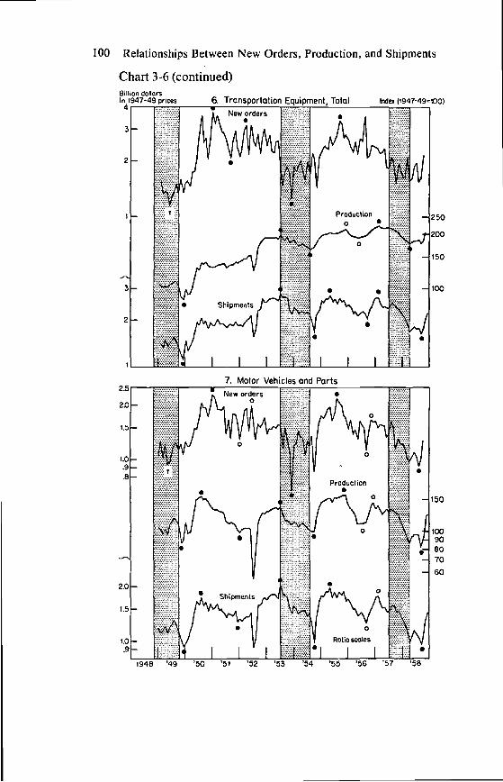
Third, the major-industry components of the durable goods sectoralso display a great deal of diversity in these respects (Chart 3-2).The difference between new orders and shipments is greater, and thefluctuations of both series are much larger, in primary metals than infabricated metal products. Orders are more erratic for electrical thanfor nonelectrical machinery and show less systematic cyclical devia-tions from shipments (persistent and large deviations for electricalmachinery are limited to the Korean War period and the 1953—54recession). Orders for transportation equipment have particularlylarge irregular movements of very short duration, which are radicallysmoothed out in shipments. This will be shown to reflect primarily therelationships in the nonautomotive component of that industry, which

Size and Frequency of Fluctuations 77
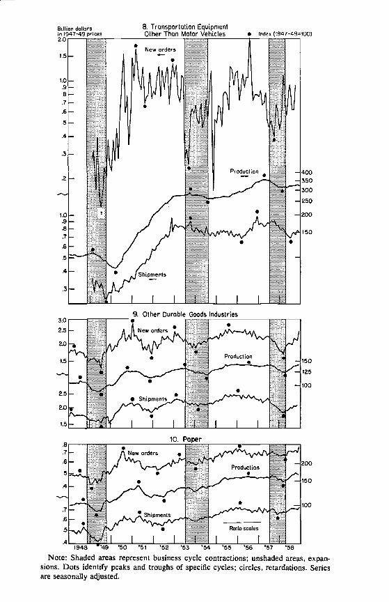
is dominated by large and expensive items (aircraft, ships, railroadequipment) that are produced to order, often with long delivery periods.The automotive component (motor vehicles and parts) shows, incontrast, only small divergencies between new orders and shipments,and behaves typically like an industry which produces primarily tostock.4 In the remaining group of "other durable goods industries"new orders and shipments also run close to each other, with shipmentsbeing smoother and lagging but slightly. This group is composed mainlyof stone, clay, and glass products, furniture, and lumber, which arelargely items made to stock or (like furniture in part) made to orderbut with rather short delivery periods.
Finally, the relations concerned have undergone certain changesover time which are reflected in our charts. In the period since 1958—60,new orders and shipments differed much less than in the previoustwelve or fourteen years covered. This implies that the changes inunfilled orders have become smaller in the first half of the 1960's.Direct evidence that this has indeed happened is given in Chapter 6,and shows that backlogs of manufacturers' orders generally havemarkedly diminishing fluctuations around downward or horizontaltrends during these latter years.
On the whole, there is a one-to-one correspondence between themajor movements in new orders and shipments, but a significantdivergence from it occurred in 1950—52. The outbreak of the KoreanWar caused a rush of forward buying motivated by fear of shortagesand price rises; this receded at the end of 1950 when hope spread thatthe conflict might end soon, but another wave of buying started whenthe war was intensified by Chinese intervention. These rises broughtnew orders to levels far above those of shipments, thus leading to avery large accumulation of unfilled orders. When new orders declinedin 195 1—52, shipments of durable goods continued to increase, thoughat a slower pace, reflecting work on the previously accumulated orders(Chart 3-1). The continued rise of shipments is particularly evident inindustries with longer average delivery periods, such as nonelectricalmachinery and (nonautomotive) transportation equipment; in contrast,shipments declined in 1951 in response to the fall in new orders in
In fact, unfilled orders of motor vehicle manufacturers are relatively small, consisting as they dolargely of military orders; the bulk of production here is represented by automobiles which areshipped to dealers who hold the inventory of finished cars.

78 Relationships Between New Orders, Production, and Shipments
industries working largely to stock or with short delivery lags, such asthe nondurables and the group of "other durables" (Chart 3-2).
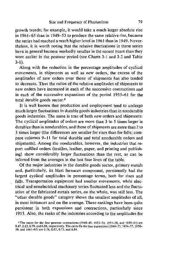
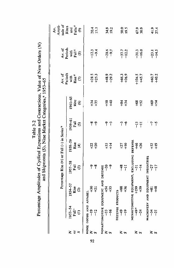
Relative Cyclical Amplitudes of the Major-Industry SeriesTable 3-1 presents percentage amplitudes of cyclical rises and falls
for the series that were presented in Charts 3-1 and 3-2. With veryfew exceptions, the current value of new orders (N) rose more in per-centage units than the value of shipments (S) in each successive ex-pansion of these series. Similarly, N as a rule fell more than S in eachof the successive specific contractions.5
Since the amplitudes of the rises are based on the initial low levelsand those of the falls on the initial high levels, the former are in asense overstated and the latter are understated. Using average cyclicallevels as bases would correct for this "bias," which should be recog-nized in reading the table. However, for our comparisons, which aimmainly at differences between variables and industries, the simplermeasures applied are deemed adequate. As the effects of the basedifferences on rises and falls tend to cancel each other, the over-allaverages taken without regard to sign (column 11) would be but weaklyinfluenced by this technical factor.
The series have upward trends and their rises are substantially largerthan their falls, as illustrated in the charts and demonstrated in themeasures of Table 3-1. This difference is real enough and quite general,even though it should be somewhat discounted because of the baseeffects just noted. More interestingly, the relative amplitudes of risesshow a tendency to decline in three successive episodes: They were onthe whole smaller in 195 8—59 than in 1954—57 and smaller in the latterperiod than in 1949—53. However, the most recent rises of the 1960's(which were still in progress at the time of this analysis), have alreadyexceeded the earlier expansions of the mid- and late 1950's, though not,in general, those of 1949—53 (compare columns 2, 4, 6, and 8). Atendency for the recent declines to become progressively smaller isalso observable in Table 3-1 (compare columns 1, 3, 5, and 7). Ofcourse, these differences themselves are in part a reflection of the
apparent exceptions are due to special causes or are not really significant. Thus the primarymetals figures for 1948—53 (Table 3-1, columns I and 2) are affected by the steel strike in 1949,which caused a lower trough level in shipments than in new orders (compare Chart 3-2). Elsewherethe differences between the amplitudes are negligible in those cases in which the movement of Sseems to exceed the movement of N (see the totals for nondurable goods in Table 3.1).
Size and Frequency of Fluctuations 79
growth trends; for example, it would take a much larger absolute risein 1961-65 than in 1949—53 to produce the same relative rise, becausethe series had reached a much higher level in 1961 than in 1949. Never-theless, it is worth noting that the relative fluctuations in these serieshave in general become markedly smaller in the recent years than theywere earlier in the postwar period (see Charts 3-1 and 3-2 and Table3-1).
Along with the reduction in the percentage amplitudes of cyclicalmovements, in shipments as well as new orders, the excess of theamplitudes of new orders over those of shipments has also tendedto decrease. Thus the ratios of the relative amplitudes of shipments tonew orders have increased in each of the successive contractions andin each of the successive expansions of the period 1953—61 for thetotal durable goods sector.6
It is well known that production and employment tend to undergomuch larger fluctuations in durable goods industries than in nondurablegoods industries. The same is true of both new orders and shipments:The cyclical amplitudes of orders are more than 3 to 5 times larger indurables than in nondurables, and those of shipments are more than 2 to3 times larger (the differences are smaller for rises than for falls; com-pare columns 9—11 for total durable and total nondurable orders andshipments). Among the nondurables, however, the industries that re-port unfilled orders (textiles, leather, paper, and printing and publish-ing) show considerably larger fluctuations than the rest, as can beinferred from the averages in the last four lines of the table.
Of the major industries in the durable goods sector, primary metalsand, particularly, its blast furnaces component, persistently had thelargest cyclical amplitudes in percentage terms, both for rises andfalls. Transportation equipment had smaller movements, while elec-trical and nonelectrical machinery series fluctuated less and the fluctu-ation of the fabricated metals series, on the whole, was still less. The"other durable goods" category shows the smallest amplitudes of all,in most instances and on the average. These rankings have been quitepersistent in both expansions and contractions, particularly since1953. Also, the ranks of the industries according to the amplitudes for
8The ratios for the four postwar contractions (1948—49, 1953—54, 1957—58, and 1959—61) are0.47,0.63,0.79, and 0.86, respectively. The ratios for the four expansions (1949—53, 1954—57, 1958—59. and 196 1—65) are 0.76, 0.67, 0.73, and 0.84.

Tab
le 3
-1Pe
rcen
tage
Am
plitu
des
of C
yclic
al E
xpan
sion
s an
d C
ontr
actio
ns, V
alue
of
New
Ord
ers
(N)
and
Ship
men
ts (
S), b
y M
ajor
Ind
ustr
ies,
194
8—65
'
.A
v.A
rnpl
i-Pe
rcen
tage
Ris
e (+
)or
Fal
l (—
)in
Ser
ies
aA
v. o
fPe
riod
sw
ith
Av.
of
Peri
ods
with
tude
of
Ris
esan
dN
1948
—49
1949
—53
1953
—54
1954
—57
1957
—58
1958
—59
1959
—61
1961
—65
orFa
llR
ise
bFa
llR
ise
Fall
Ris
eFa
llR
ise
cR
ise
dFa
ll d
Falls
dS
(1)
(2)
(3)
(4)
(5)
(6)
(7)
(8)
(9)
(10)
(11)
AL
L M
AN
UFA
CT
UR
ING
IND
US
TR
IES
N—
20+
72—
17±
36—
12+
26—
8+
50+
46.0
—14
.330
.2S
—14
+64
—10
±29
—11
+20
—6
+44
+39
.4—
10.0
26.7
DU
RA
BLE
GO
OD
S IN
DU
STR
IES,
TO
TA
LN
—32
+13
5—
27+
57—
24+
41—
14+
63+
73.7
—24
.649
.1S
—15
+10
2—
17+
38—
19+
30—
12+
53+
55.7
—15
.735
.8
PRIM
AR
Y M
ET
AL
S, T
OT
AL
N—
38+
97—
47+
128
—48
+11
0—
42+
76+
102.
7—
43.9
73.3
S—
40+
132
—30
+68
—36
+54
—28
+50
+76
.2—
33.6
54.9
BL
AST
FU
RN
AC
ES,
ST
EE
LM
ILL
S
Nn.
a.n.
a.—
53+
175
—58
+16
6—
58+
118
+15
3.1
—53
.710
4.7
Sn.
a.n.
a.—
38+
94—
43+
71—
37+
68+
77.7
—39
.658
.7
FAB
RIC
AT
ED
METAL PRODUCTS
N—
33+102
—27
+54
—14
+24
—10
+40
+55.0
—21.0
38.0
S—
16+
80—
14+
37—
12+
18—
8+
31+
41.4
—12
.527
.0

EL
EC
TR
ICA
L M
AC
HIN
ER
Y
N—
22+
155
—42
+81
—18
+34
—4
+69
+84
.6—
21.4
53.0
S—
12+
120
—21
+29
—13
+32
—1
+59
+60
.1—
11.8
35.9
MA
CH
INE
RY
, EX
CE
PT E
LE
CT
RIC
AL
N—
21+
100
—26
+68
—24
+33
—11
+76
+69
.3—
20.4
44.9
S—
18+
93—
19+
42—
12+
18—
6+
57+
52.5
—13
.933
.2
TR
AN
SP
OR
TA
TIO
NE
QU
IPM
EN
T
N—
12+
140
—30
33+
40—
18+
87+
89.6
—23
.156
.3S
—13
+12
2—
18—
24+
32—
12+
63+
66.8
—17
.041
.9
OT
HE
RD
UR
AB
LE
GO
OD
S IN
DU
STR
IES
N—
16+
84—
21+
23—
12+
27—
9+
46+
44.8
—14
.729
.8S
—10
+62
—14
+19
—10
+22
—7
+40
+35
.9—
10.4
23.1
TO
TA
LN
ON
DU
RA
BL
E G
OO
DS
IND
UST
RIE
SN
—11
+34
—5
+22
—2
+12
—0.
1+
36+
27.6
—4.
515
.2S
—12
+33
—4
+23
—3
+12
+0.
3+
35+
25.4
—4.
815
.1
TO
TA
LN
ON
DU
RA
BL
ES
WIT
H U
NFI
LL
ED
N—
16+
52—
11+
26—
6+
21—
5+
50+
37.1
—9.
623
.3S
—16
+40
—8
+23
—5
+16
—3
+46
+31
.5—
8.0
19.8
82 Relationships Between New Orders, Production, and Shipments
Notes to Table 3-1
Note: The amplitude measures in columns 3—8 for all industries and those in columnsI and 2 for all manufacturing, total durable goods, and total nondurable goods industriesare based on the new Census data (1963 revision). For the other industries, themeasures in columns 1 and 2 are based on the earlier OBE data (the revised series forthe component industries begin in 1953).
8 The annual dates given refer to the expansions and contractions in total manufac-turers' shipments. The corresponding movements in the component series may havedifferent dates. As a rule, the amplitude of each successive rise and fall in the given seriesis measured between the average standings of the seasonally adjusted series in the three-month periods centered on the initial and terminal turns, and all amplitudes are ex-pressed in percentages of the initial-turn levels. However, the high levels attained bythe series late in 1965 were used as terminal values for the measured amplitudes of1961—65 (column 8), even though the expansions apparently still continued at the timethis analysis was being performed; hence these figures refer to truncated movements andin this sense understate the (currently unknown) "true" amplitudes of the rises thatbegan in 1960—61.
b In this period, new orders for durable goods rose to steep peaks in 1950—5 1 ,then de-clined sharply in 1951, finally increased erratically and moved slowly in 1952 (seeCharts 3-1 and 3-2). For some industries, these movements can be matched with thoseof shipments. To make the results for the different industries more comparable, ampli-tude measures for these additional movements are not included in the table, but they areshown below:
Fabricated OtherTotal Primary Metal Durable
Durable Metals Products Goods
N S N S N S N S
1949—51 rise +87 +52 +111 +110 +172 +61 +87 +521951—52 fall —22 —12 —36 —41 —38 —6 —22 —12
Significant retardations interrupted these rises in 1962 in several major industries(see Charts 3-1 and 3-2). The following tabulation illustrates the magnitudes of themovements involved.
Fabri-cated
All Manu- Total Primary Blast Metalfacturing Durable Metals Furnaces Products
N S N S N S N S N S
1961—62 rise +14 +14 +22 +20 +64 +33 +82 +28 +16 +71962'fall —2 4 —2 —27 —13 —38 —18 —4 3
d The averages in column 11 are taken without regard to sign, but not those in columns9 and 10. Because of rounding, the figures shown may differ from ones computed di-rectly from the listings in columns 1—8.
(continued)

Size and Frequency of Fluctuations 83
Notes to Table 3-i (concluded)
Short but substantial declines interrupted these rises in 1955—56 (see Chart 3-2).The amplitudes of the increases that started in 1953—54 and ended in 1955 were +82and +42 for new orders and shipments, respectively; those of the declines in 1955—56were —18 and —14.
Includes stone, clay, and glass products; lumber and wood products; furniture; instru-ments and related products; and miscellaneous, including ordnance.
g Includes textile mill products; leather and leather products; paper and alliedproducts; and printing and publishing.
new orders and shipments have tended to be remarkably similar:the Spearman rank correlation coefficients (rR) exceed .85 for each ofthe six periods with rise or fall in 1953—65. The correlations betweenthe ranks based on average amplitudes are perfect (r8 = 1) for rises andfor rises and falls combined, while the correlation for falls is .86.
The high degree of cyclicality and volatility of new orders receivedby such industries as iron and steel, transportation equipment (particu-lary nonautomotive), and machinery, confirms the long-held idea thatinvestment demand is often very unstable. While shipments (and out-put) fluctuate much less than new orders, they nevertheless vary con-siderably more in these industries than elsewhere in the manufacturingsector. And it is in these industries that production is to a large extentorder oriented, resulting in order leads of substantial analytical andpredictive interest.
Market CategoriesFor the new Census series, industry data have been regrouped into
major market sectors covering consumer goods, equipment, andmaterials. The composition of these "market categories" followsbelow.7
Home goods and apparel: Knitting and floor covering mills; apparel;household furniture and fixtures; leather products (other than indus-trial and cut stock); kitchen articles and pottery; cutlery, handtools,and hardware; household appliances; ophthalmic goods, watches, andclocks; and miscellaneous personal goods.
Consumer staples: Food and beverages; tobacco manufactures; die-
7This is a short description; for a detailed listing of the SIC industries included, see Census,Manufacturers' Shipments (Revised), App. B.

84 Relationships Between New Orders, Production, and Shipments
cut paper and board; newspapers, periodicals, and books; and drugs,soaps, and toiletries.
Equipment and defense items, except automotive: Furniture andfixtures, other than household; machinery, electrical and other (ex-cluding household appliances and some others); aircraft, shipbuilding,railroad and streetcar equipment; scientific and engineering instru-ments; and ordnance.
Automotive equipment: 8 Motor vehicles and parts; motorcycles,bicycles, boat building, trailer coaches; and tires and tubes.
Construction materials, supplies, and intermediate products: Woodproducts (except containers); building paper; paints; paving androofing materials; stone, clay, and glass products (other than kitchenarticles, pottery, and glass containers); and building materials (fabri-cated metals) and Wire products.
Other materials and supplies and intermediate products: Fats andoils; broad-woven fabrics and other textiles (except those in homegoods and apparel); wooden and glass containers; pulp, paperboard,and other paper products; printing and publishing (except the itemsin consumer staples); chemicals and allied products: industrial,fertilizers, and miscellaneous; petroleum and coal products (exceptpaving and roofing materials); rubber and plastics (except tires andtubes); leather, industrial products, and cut stock; primary metals;fabricated metal products: cans, barrels, and drums, and others n.e.c.;internal combustion engines; machine tools and machine shops; elec-trical industrial apparatus, electronic components, and other electricalmachinery n.e.c.; aircraft parts; photographic goods, watch cases; andother durable goods, except personal and ordnance.
In short, these groupings provide both a division between finalproducts and materials and a further division of final products betweenconsumer goods and equipment for business and government use.
In addition, data for the following three "supplementary marketcategories" are available (for consumer durables only since 1960):
Consumer durables: Same as home goods and apparel (above),except that knitting and floor covering, apparel, and the leather prod-ucts are excluded.
This is treated as a separate market grouping, instead of being divided between consumer goods,equipment (buses and trucks), and materia!s (motor vehicle parts), because the Industry Surveyreports do not separate the value of cars and trucks.
Size and Frequency of Fluctuations 85
Defense products: Communication equipment; complete aircraft;aircraft parts; and ordnance (part of group 3 above).
Machinery and equipment industries: Machinery, except electrical(excluding farm machinery and machine shops); electrical machinery(excluding household appliances, communication equipment and elec-tronic components); shipbuilding; and railroad and streetcar equipment.
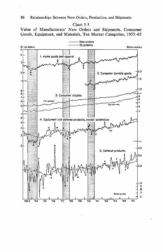
Chart 3-3 presents the seasonally adjusted series on new orders andshipments for each of the nine market categories just described as wellas for total materials (which includes the "Construction materials"and "Other materials . . ." groups identified above). It is clear that thegoods purchased by the consumer are overwhelmingly made to, andsold from, stock. New orders and shipments of these classes of goodsmove closely together and show very small, and for the most partapparently random, differences. In particular, N and S are virtuallyidentical for consumer staples. The two variables are somewhat moredifferentiated for home goods and apparel, but here too the deviationsare generally small, except during the decline and initial rise associatedwith the 1953—54 recession. The series for consumer durables are veryshort, since they begin in 1960. They closely resemble their counter-parts for the home goods group, which covers the same productsalong with some nondurables.
In contrast, the equipment series cover in large part goods manu-factured to order, and the picture they present is very different. In1953—58, particularly, new orders for nonautomotive equipment anddefense products moved in much wider swings than shipments, whichalso lagged behind the orders by long intervals. In 1959—62, a periodmarked mostly by sluggish increases and retardations in these series,the deviations between N and S became considerably smaller andpredominantly erratic; but in 1963—65, when business moved up morebriskly, new orders again repeatedly rose faster than shipments, onlyto fall back occasionally to the level of the latter. Throughout, ship-ments of equipment have followed a much smoother course than thehighly volatile orders. New orders for defense products have beenespecially erratic, moving up and down in large seesaw patterns everyfew months. However, longer movements superimposed upon thoseirregular oscillations are also evident in the defense series during the1950's. The timing of these movements was unfavorable as far as thebusiness cycle is concerned: defense orders declined sharply just be-
86 Relationships Between New Orders, Production, and Shipments
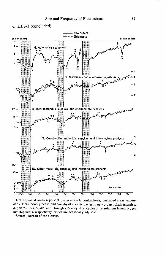
Chart 3-3Value of Manufacturers' New Orders and Shipments, ConsumerGoods, Equipment, and Materials, Ten Market Categories, 1953—65
1953 '54 '55 '56 '57 '58 '59 '60 '6$ '62 '63 '64 '65
New ordersShipments
Size and Frequency of Fluctuations 87
Chart 3-3 (concluded)
dollars
New ordersShipments
Billion dollars
£
a
I
A
1v,_,'j/
7.
£
20
6 Automotive eqwpmentAs ::::•:•:•:•::•:•
—
9 Consiruclton materials, supplies, and intermediate products
10 Other malertals, supplIes, and intermediate products••
ill, to scales
5
4
3
2
4
3
2
20
1098
1953 '54 '55 '56 '57 '58 '59 '60 '61 '62 '63 '64 '65
Note: Shaded areas represent business cycle contractions; unshaded areas, expan-sions. Dots identify peaks and troughs of specific cycles in new orders; black triangles,shipments. Circles and white triangles identify short cycles or retardations in new ordersand shipments, respectively. Series are seasonally adjusted.
Source: Bureau of the Census.

88 Relationships Between New Orders, Production, and Shipments
fore and during the 1953—54 recession and again in 1956—57, prior tothe downturn of aggregate economic activity in mid-1957. The recent(1963—65) increase in the short-period volatility of total equipmentorders is also to a considerable extent (though by no means exclu-sively) due to renewed large variations in defense orders (see Chart3-3).
The series for machinery and equipment industries represent trans-actions related to the business outlays on "producer durable equip-ment." They share much of their coverage with the correspondingseries for nonautomotive equipment (other than defense products),but include also some types of machinery classified as components ofthe market group "Other materials and supplies and intermediateproducts." On the whole, new orders of the machinery and equipmentindustries are apparently smoother than new orders for total non-automotive equipment and defense products, but the longer cyclicalmovements in these series are similar.
Unlike nonautomotive transportation equipment (aircraft, ships,railroad equipment), which is produced to order, usually with long lagsof output and shipments behind new orders, motor vehicles are madelargely to stock. The graph for automotive equipment shows N and Smoving .closely together most of the time (Chart 3-3), while the cor-responding series for total transportation equipment differ by largeamounts (Chart 3-2). Automotive orders follow a course that is only alittle less smooth than that of shipments, while total transportationequipment orders are, in contrast to shipments, very erratic. Thisimplies, of course, that new orders for transportation equipmentexcluding automobiles are even more erratic, and this is evident inthe older data, which do distinguish between "motor vehicles andparts" and "other transportation equipment" (see Chart 3-4). But thecharts suggest, too, that the divergence between the time paths of Nand S for nonautomotive (and total) transportation equipment is in partalso cyclical, i.e., reflected in longer and systematic movements, notjust in very short irregularities.
Other evidence, on timing and on size of unfilled orders (Chapters 4and 6), will confirm these statements. Meanwhile, let us merely notethat motor vehicle manufacturers hold relatively small amounts of
° New orders for these industries will be used extensively in Part IV, below.
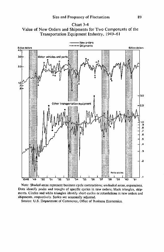
Size and Frequency of Fluctuations 89
Chart 3-4Value of New Orders and Shipments for Two Components of the
Transportation Equipment Industry, 1949—61
f'Jew ordersShipments
Billion dollars BiliLon dollars—Motor vehicles and parts
So £ L
A£
20 i'.' I
AIi
OA 0I
t,l
a
9 A
6a
. 30
Other transportation equipment2 0
A
3
A 2
scales
— I I I I _11948 '49 '50 '51 '52 '53 '54 '55 '56 '57 '58 '59 '60 '61
Note: Shaded areas represent business cycle contractions; unshaded areas, expansions.Dots identify peaks and troughs of specific cycles in new orders; black triangles, ship-ments. Circles and white triangles identify short cycles or retardations in new orders andshipments, respectively. Series are seasonally adjusted.
Source: U.S. Department of Commerce, Office of Business Economics.

90 Relationships Between New Orders, Production, and Shipments
unfilled orders (for most of them the reported backlog figures are con-fined to military orders). The bulk of their production is represented byautomobiles shipped to dealers, who then hold the finished car inven-tory for sale. Although cars come in a great variety of models, colors,and combinations of accessories, among which the buyer may chooseas he wishes, individual customer specifications, as communicated tothe dealer, are as a rule readily met by producers, without any signifi-cant delays in delivery.
It should be added that, according to the old series (Chart 3-4), neworders for motor vehicles did have much larger amplitudes than ship-ments in the years 1951—54, which include the Korean conflict andits aftermath. If this was so, it is possibly due in large part to militaryorders; but it seems idle to speculate about the matter, especially sincethe quality of these data is quite uncertain. In any event, after 1955 thetwo series, even according to the old data, show little difference inamplitudes and nearly coincident timing.'°
Of the two parts of "materials, supplies, and intermediate products"(Chart 3-2), the group relating to construction had somewhat largerirregular, but smaller cyclical, fluctuations than the other, much largergroup. The latter includes the highly cyclical metalworking industries,which is clearly reflected on several occasions, such as the long lead ofnew orders relative to shipments for this group at the 1953—54 upturns(compare the corresponding graphs in Charts 3-2 and 3-3).
Relative Cyclical Amplitudes of the Market-Category SeriesTable 3-2 presents for the market groups the same information on
the size of successive cyclical movements in new orders and ship-ments as Table 3-1 gave for the major industries." The format is inboth cases the same, and so is the general observation that N rises andfalls more than S for each of the groups, with great regularity.
Comparisons of the amplitudes recorded in the different subperiodsalso merely yield a confirmation of what has been noted before: The
series for motor vehicles and parts in Chart 3-4 show much more erratic behavior in1953—61 than do the corresponding series for total automotive equipment in Chart 3-3. While thelatter data represent a somewhat larger aggregate, this difference may be due more to the smallersize of the samples underlying the older data in Chart 3-4. The cyclical movements, however, arebroadly similar in the two charts, which is reassuring about the internal consistency of this evidence.
" Two categories, consumer staples (1953—65) and consumer durables (1960—65), are not in-cluded in this table. As seen in Chart 3-3, these series are dominated by upward trends and show noidentifiable cyclical fluctuations.

Size and Frequency of Fluctuations 91
declines tend to become smaller, while the latest rises already rivalthose of 1954—57 (the rises of 1958—59 were definitely the smallestbut also the shortest in the recent years). Again, increases in the am-plitude ratios S/N are frequently observed, as illustrated by the fol-lowing results for home goods and apparel (HG), nonautomotive equip-ment and defense (NAE), machinery and equipment industries (ME),and total materials, supplies, and intermediate products (MSI).
Fall HG NAE ME MSI Rise HG NAE ME MSI1953—54 0.63 .48 .62 .50 195,4—57 0.70 .65 .59 .681957—58 0.89 .45 .63 .83 1958—59 0.91 .40 .59 .871959—61 1.25 .33 .71 .91 1961—65 1.03 .69 .78 .88
The group of home goods and apparel has the smallest cyclical risesand falls in both new orders and shipments. Moving on to progressivelylarger average percentage amplitudes, construction materials andother materials rank second and third for new orders, followed byautomotive equipment, defense products, and nonautomotive equip-ment. The rankings for shipments are similar,'2 but they differ in tworespects from those for new orders: the ranks of defense products areconsistently lower for S and the ranks of automotive equipment areconsistently higher. This reflects two facts: (1) The production smooth-ing process is highly effective for the defense items, which have largebacklogs and long delivery periods (the amplitudes of N are here, onthe average, about two and a half times larger than those of S); and(2) in contrast, there is very little smoothing, if any, in the automotivegroup.
In short, the fluctuations of both new orders and shipments tend tobe smallest for consumer goods, larger for materials (particularly the"Other materials" group, which includes the sensitive metalworkingindustries), and by far the largest for equipment. The groups withgreater relative amplitudes are also, on the whole, the groups withgreater weights of products manufactured to order. However, as animportant special case, the automotive category represents a segmentof the economy where the demand is highly variable but production isnot "to order" in the sense used here. For this category, current pro-
12The r9 coefficients are .77 for periods of rise, .60 for periods of fall, and .7! for all six episodesin 1953—65.
Tab
le 3
-2Pe
rcen
tage
Am
plitu
des
of C
yclic
al E
xpan
sion
s an
d C
ontr
actio
ns, V
alue
of
New
Ord
ers
(N)
and
Ship
men
ts (
S), N
ine
Mar
ket C
ateg
orie
s,a
1953
—65
Av.
Am
pli-
Perc
enta
ge R
ise
(+)
or F
all (
—) i
nS
erie
s b
Av.
of
Peri
ods
with
Av.
of
Peri
ods
with
tude
of
Ris
esan
dN
1953
—54
1954
—57
1957
—58
1958
—59
1959
—61
1961—65
orFa
licR
ise
Fall
Ris
eFa
llR
ise
Ris
edFa
lidFa
lls'
S(1
)(2
)(3
)(4
)(5
)(6
)(7
)(8
)(9
)
HO
ME
GO
OD
S A
ND
APP
AR
EL
—19
+30
—9
+22
—8
+34
+28
.5—
12.3
20.4
S—
12+
21—
8+
20—
9+
35+
25.3
—9.
417.3
NONAUTOMOTIVE
EQ
UL
PME
NT
AN
D D
EFE
NSE
N—
33+54
—20
+35
—9
+58
+48
.9—
20.8
34.9
S—
16+
35—
9+
14—
3+
40+
29.2
—9.
719
.2
DE
FEN
SE P
RO
DU
CT
SN
—49
+88
—48
+27
—3
+84
+66
.3—
33.7
50.0
S—
19+
36—
11+
10—
6+
34+
26.9
—12
.219
.5
NO
NA
UT
OM
OT
IVE
EQ
UIP
ME
NT
, EX
CL
UD
ING
DE
FEN
SEN
_49e
+19
9—
31+
46—
13+
68+
104.
5—
31.3
67.9
S—
24+
59—
14+
26—
11+
52+
45.7
—16
.030
.9
MA
CH
INE
RY
AN
D E
QU
IPM
EN
T I
ND
UST
RiE
SN
—34
+81
—27
+32
—7
+69
+60
.7—
23.1
41.9
S—
21+
48—
17+
19—
5+
54+
40.2
—14
.527
.4
AU
TO
MO
TIV
E E
QU
IPM
EN
T
N—
16—
34+
69—
22+
88+
69.5
—23
.946
.7S
—22
—32
+65
—23
+83
+65
.6—
25.6
45.6
MA
TE
RIA
LS,
SU
PPL
IES,
AN
D I
NT
ER
ME
DIA
TE
PR
OD
UC
TS
N—
24+
47—
18+
31—
11+
42+
40.1
—17
.328
.7
S—
12+
32—
15+
27—
10+
37+
32.4
—12
.422
.4
CO
NST
RU
CT
ION
MA
TE
RIA
LS,
ET
C.
N—
17+
41—
15+
29—
12+
33+
34.3
—14
.624
.5S
—7
+31
—10
+23
—12
+31
+28
.1—
9.5
18.8
OT
HE
R M
AT
ER
IAL
S, E
TC
.N
—21
+45
—19
+33
—11
+47
+41
.7—
17.1
29.4
S—
12+
33—
16+
29—
10+
40+
33.9
—13
.123
.5
aF
orco
mpo
sitio
n of
thes
e ca
tego
ries
, see
text
.b
See
Tab
le 3
-1, n
ote
a.T
he h
igh
leve
ls f
rom
whi
ch th
ese
seri
es s
tart
in 1
953
wer
e us
ed a
s th
e ba
se f
or th
e m
easu
res
in th
is c
olum
n, e
ven
whe
re s
uch
leve
lsca
nnot
be p
ositi
vely
iden
tifie
d as
spe
cifi
c-cy
cle
peak
s.d
The
aver
ages
in c
olum
n 9
are
take
n w
ithou
t reg
ard
to s
ign,
but
not
thos
e in
col
umns
7 a
nd 8
. Bec
ause
of
roun
ding
, the
fig
ures
sho
wn
may
diff
er f
rom
one
s co
mpu
ted
dire
ctly
fro
m th
e lis
tings
in c
olum
ns 1
—6.
oR
efer
sto
the
decl
ine
in th
e se
cond
hal
f of
195
3, w
hich
inte
rrup
ted
the
very
larg
e ir
regu
lar
mov
emen
ts in
the
firs
t hal
f of
the
year
(se
eC
hart
3-3
).°T
here
are
add
ition
al m
ovem
ents
in th
ese
seri
es. T
o m
aint
ain
com
para
bilit
y w
ith th
e ot
her
grou
ps, t
hese
mov
emen
ts a
re n
ot in
clud
ed in
the
tabl
e. T
he a
mpl
itude
s of
the
shor
t but
ste
ep r
ises
in 1
954—
55 w
ere
+73
in n
ew o
rder
s an
d +
64 in
shi
pmen
ts; t
hose
of
the
ensu
ingd
e-cl
ines
in 1
955—
56 w
ere
—26
and
—24
; and
thos
e of
the
rise
s in
195
6—57
wer
e +
18 a
nd +
19 (
com
pare
Cha
rt 3
.3).
Had
thes
e m
easu
res
been
in-
clud
ed, t
he a
vera
ges
in c
olum
ns 7
—9
for
mac
hine
ry a
nd e
quip
men
t ind
ustr
ies
wou
ld h
ave
been
som
ewha
t sm
alle
r (+
61.7
, —24
.3, a
nd 4
3.0
for
new
ord
ers;
and
+57
.6, —
25.0
, and
41.
3 fo
r sh
ipm
ents
).

94 Relationships Between New Orders, Production, and Shipments
duction operations, as measured by shipments, follow quite faithfullythe large short-term variations in demand, as measured by new orders.
Series in Constant PricesIn undertaking to compare new orders with production, one is con-
fronted with a major gap in the data: the unavailability of aggregatevolume estimates for new orders. In an attempt to bridge this gap, wehave corrected the Department of Commerce estimates of the currentvalue of manufacturers' new orders for changes in prices. This adjust-ment was applied to the major industry series in the OBE compilationfor the years 1948—58; at the time, the revised Census data were notyet available. The deflating indexes used for these corrections are es-sentially combinations of the appropriate components of the Bureau ofLabor Statistics wholesale price index.
Deflation procedures, even when carefully executed, seldom pro-duce more than crude approximations, for the difficulties and pitfallsare many. Without fully describing at this point the procedures anddata employed,13 two special problems are discussed. The first con-cerns the timing of orders and price data; the second, the pricing ofgoods made to specific orders.
To the extent that manufactured products are priced at the time theorders for them are received and accepted, it is precisely to the new-order series that the current price indexes would be applicable as de-flators. Clearly, too, where the products so priced are not shippedimmediately but require some time for production and delivery, thesame indexes would often fail to be properly applicable as deflators ofthe data on the value of output or shipments. For the latter would thenbe recorded at the price of the period in which the order was acceptedrather than at the price of the period in which the order was delivered,and the two may well differ. Of course, for new orders shipped fromstock, whose value equals that of shipments of the same period, nocomplications of this sort can arise; as a rule, the current price is theright one to use for both the new order and the sales series.
What if the price was not contractually fixed at the time the orderhad been accepted? Where time-consuming production processes areinvolved, the long-term contract may provide that the price of the out-put shall be adjusted according to the changes in the input prices during
13 See Appendix C.

Size and Frequency of Fluctuations 95
the period set for the completion of thç order. Such escalation pro-visions, based as a rule on the BLS wholesale price index, are commonin certain industries.'4 In such cases, the precise contract sum (price ofthe preordered output at the time the order is accepted) is unknown.But if no other price has been specified at that time, then the price ofthe current (i.e., the order-acceptance) period can be presumed toapply; any subsequent price changes canBot, and need not, be takeninto account in a deflation procedure whose aim can only be correctionfor current, not future, price changes.
Conceptually, then, the only real difficulty seems to be with thosenew orders that are contracted for at price levels different from thoseprevailing in the current period. This need not cause serious difficultyin practice.
The difficulty of pricing custom-made equipment gives rise to animportant deficiency of the price data. The wholesale price indexesmeasure essentially the price movements in primary markets, wherethe goods are first sold commercially, ordinarily in large lots. But thereis no "market price" in this sense for unique products, that is, for goodsmade to order and designed to meet individual customer specifications,such as planetarium equipment or an airliner. Although many of thetechnical or quality characteristics of such products may have a com-mon valuation which they implicitly contribute to the product's trans-action price, this price may vary with each buyer, since each purchaseis likely to involve a different bundle of product attributes. The BLShas not found it possible to price directly such items as "ships andrailroad stock, fabricated plastic products, and some machinery whichis largely custom-made." 15
The series of manufacturers' new orders in constant (average 1947—49) prices are presented in Chart 3-5 for the comprehensive industrygroups and in Chart 3-6 for the major component industries. Theseseries show much weaker upward trends than their undeflated counter-
Cf. M. E. Riley, "The Price Indexes of the Bureau of Labor Statistics," in The Relationship ofPrices to Economic Stability and Growth, Compendium of Papers Submitted by Panelists Appear-ing before the Joint Economic Committee, 85 Cong., 2nd sess., Washington, D.C., 1958, P. 114. Theauthor notes that "virtually all of the heavy power-generating equipment produced is made under anarrangement by which the contract sum is adjusted for changes in the prices of selected materials andcomponents between the initiation and completion of the job. Federal shipbuilding contracts con-tain similar provisions."
"Wholesale Price Index," in U.S. Bureau of Labor Statistics, Techniques of MajorBLS Statistical Series, BLS Bulletin 1168, Washington, D.C., 1954, p. 84.
On the construction of price deflators for the industries not covered in the BLS data (such as non-automotive transporation equipment and printing and publishing), see Appendix C.

96 Relationships Between New Orders, Production, and Shipments
Chart 3-5New Orders and Shipments in Constant Dollars and Production
Indexes, All Manufacturing, Durable and Nondurable GoodsIndustries, 1948—58
BLII(on dollarsin t947-49 prices 1. All Manufacturing Industries Index (1947-49:100)
26— F • F I • I
I .1 1...20 — I
JV New orders
• 'I16
14—1 .1 4 1 J
—150
I IProduction
I,.#' o — 110
F 1-10026—
F •11-90— I I Shipments I
20:1 1 A
18 JI I I I I I
2. Durable Goods Industries164: i . F E i
— New orders12-- S10 —9—
S
7-6 — Produciton • —170
0
0 —110—100
12— • —90Shipments 8010- 0
9—
o7—6 — Ratio scales
I I I I I
1948 '49 '50 '51 '52 '53 '54 '55 '56 '57 'SB

Size and Frequency of Fluctuations 97
Chart 3-5 (concluded)Billion dollors(n 1947-49 prices 3. Nondurable Goods Industries Index 100)16 .•.•..w.i14:1 1 F •I I
— • New orders12— 0
10.... .:::::.:::.:.:.:::.:.
9— * Production — 1408- :120
— 110S . —100
14— —9012 — : Shipments
10—
— 1
44. Nondurable Goods Industries Reporting Unfilled Orders
36 = I Pt New orders F I32— Il A .1 A I I
20 — bk/I ] VF Production r 1
— 150
— 1 I • .1 1
• T.-iio• • -100
5. Nondurable Goods Industries Not Reporting Unfilled Orders
1948 '49 '50 '51 '52 '54 '55 '56 '57 '58
Note: Shaded areas represent business cycle contractions; unshaded areas,expan-sions. Dots identify peaks and troughs of specific cycles; circles, retardations. Series areseasonally adjusted.
98 Relationships Between New Orders, Production, and Shipments
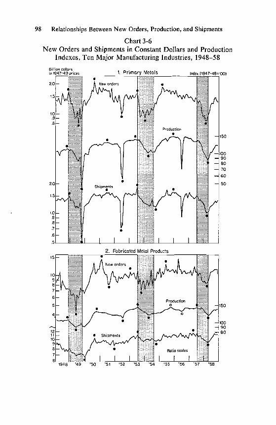
Chart 3-6New Orders and Shipments in Constant Dollars and Production
Indexes, Ten Major Manufacturing Industries, 1948—58
Billion dollarsLii I. MeI&s
2. Fabricated Metal Products

Chart 3-6 (continued)
3. Muchi
200
150
10090
150
1009080
250
200
150
Including Electrtcal Index (1947-49=100)
100 Relationships Between New Orders, Production, andShipments
Chart 3-6 (continued)StIlion dollarsin 1947-49 prices 6. Trol4
Index (1 947-49=100)
Note: Shaded areas represent business cycle contractions; unshaded areas, expan-sions. Dots identify peaks and troughs of specific cycles; circles, retardations. Seriesare seasonally adjusted.
8. Tronsportetion EquipmentOther Than Motor Vehicles • Index (1947-49=100)
'55 '56 '57 '58

102 Relationships Between New Orders, Production, and Shipments
parts, which would, of course, be expected in view of the tendency forindustrial prices to rise during most of the period covered. The short-term movements, on the other hand, were largely unaffected by theadjustment. The reason for this is that the price deflators are verysmooth and stable, while the new-order series to which they were ap-plied are much more volatile.
The observed differences in cyclical behavior between the corre-sponding constant-price series and current-price series are largely ofthe kind to be expected as a result of trend elimination. Thus, the ampli-tudes of the specific-cycle expansions tend to be somewhat smallerthan those in the constant-price series. On the other hand, cy-clical declines are often larger in the deflated than in the undeflatedfigures, but these differences are neither considerable nor system-atic.
In addition to new orders in real terms, ChartF 3-5 and 3-6 show, foreach of the major industries or groups covert I, the correspondingseries on output and real shipments. Output is represented by the ap-propriate components of the monthly Federal Reserve Index of In-dustrial Production (1953 revision, 1947—49 = 100).16 The series forshipments were constructed by deflating the OBE current-value fig-ures by means of the same price indexes that were used to deflate neworders. To the extent that prices actually changed during the deliveryperiods, this clearly results in errors for goods which were made toorder and priced as of the period in which they were ordered. On theother hand, in some cases current price deflators might apply better toshipments than to new orders; and in production to stock they shouldapply equally to both. In any event, there is no good practical alterna-tive to the simple current-price deflation procedure we have adopted;any more elaborate method would merely be pretentious, for it wouldhave to be based on necessarily arbitrary assumptions about the timeaspects of pricing the made-to-order goods.
For production, as for new orders and shipments, revised data became available after this analy-sis was completed. Examination of the new series indicates that our findings would not be materiallyaffected by the use of the revised data.
Indexes for three industry groups (other durable goods and nondurable goods industries with andwithout unfilled orders) were computed by combining the Federal Reserve indexes for the compo-nent industries with weights derived from the 1947 value added weights used in the FRB compilation.Separate indexes for automotive and other transportation equipment were obtained through thecourtesy of the Federal Reserve Board for the period before 1956, the year in which the publishedseries for these industries begin.

Size and Frequency of Fluctuations 103
Relative Movements of Real New Orders,Output, and Real Shipments
Major fluctuations in quantities ordered are typically reproduced,with lags, in the course of output, so that the phase-to-phase corre-spondence between these series is strong. But the cyclical movementsare systematically larger in real new orders than in the correspondingoutput, and these differences are particularly pronounced for the dur-able goods industries.
The sequence of corresponding cycles in new orders and productionmay be interrupted by a wave of advance buying characterized through-out by an excess of the ordering rates over the capacity output rates.The statistical expression of a concentrated buying movement of thissort would be an "extra" cycle in new orders, absorbed largely by agradual expansion of output and to a certain extent also by cancella-tions. Our materials include a single but very significant episode il-lustrating such developments: the 1950—5 1 phase of the Korean Waras experienced by a large segment of durables manufactures. The chartfor the durable goods sector as a whole shows production moving alonga virtually horizontal plateau in the last quarter of 1950 and the firsthalf of 1951, in contrast to new orders (measured net of cancellations),which first climbed to unprecedented peak levels in August 1950 andagain in January 1951, then declined steeply through the first quarter of1951. The principal point, here is that throughout this period new or-ders were received at high rates exceeding those of current shipments,and the behavior of shipments mirrored that of production. New ordersnever fell below the level of shipments; so their contraction merelyreduced the rates at which the backlog of unfilled orders, already verylarge, continued to increase. Total output of durables dipped onlyslightly in the summer of 1951, when the decline in new orders wasnearly completed, but it remained close to its top levels and soonstarted moving gradually upward again, reflecting the upturn in buy-ing in the last quarter of the year. After the mid-1952 steel strike,finally, the expansion of output resumed a more vigorous pace, feedingon the backlog which was then at its peak level, even though the re-covery of new orders was only moderate and quite hesitant throughout.Thus both the huge 1950—5 1 humps and the irregular 195 1—52 rise innew orders were translated into an almost continuous and gradual ex-pansion of output.

104 Relationships Between New Orders, Production, and Shipments
Chart 3-6 suggests that these developments, which show up well onthe graph for the total durable goods sector, are attributable mainlyto nonelectrical machinery and transportation equipment (other thanmotor vehicles). In the other major component industries of the sector,the "Korean" cycles in quantities ordered did reappear in the time pathof production, although in a strongly subdued form.
The cyclical paths of real shipments are closely similar to those ofoutput of the corresponding durable goods industries, in both ampli-tude and timing. For a technical reason, output indexes overstate thedegree to which the short irregular movements of new orders aresmoothed out in scheduling production; the series on shipments involveless rounding and therefore retain more of the erratic componentsthan do the output indexes.'7 This, however, is about the only majorand persistent difference between the charted production indexes anddeflated shipments series that the eye can detect.
A difficulty arises at this point because many of the individual in-dustry components of the Federal Reserve production indexes arebased in part on data for shipments. One saving feature is that ship-ments are often combined with inventory changes to get deflated value-of-output data. Also, the use of Census value data (after deflation) ismostly limited to the estimation of the annual indexes, whereas themonthly intrayear movements are based largely on the BLS man-hourdata. Nevertheless, the close similarity of output indexes and deflatedshipments in our charts is doubtless in some part a statistical artifactdue to the incorporation of the shipments data in the production in-dexes. This is more true for the longer trends than for the shortermovements, with which I am primarily concerned, and it is also moretrue for some industries than for others.'8
The contrast between real new orders on the one hand and outputand real shipments on the other is well expressed in the two metal-working and the two machinery-producing industries, but it is particu-larly strong in transportation equipment. This is due primarily to the
'7The Federal Reserve production indexes that are used are rounded off in a relatively drasticmanner, to exclude fractions of an index point. The OBE series, on the other hand, are expressed inmillions of dollars, while a monthly value of new orders or shipments will run into billions of dollars;as a result, the minimum changes in these series are many times smaller than those that can be ex-pressed by the production indexes.
18 Production indexes for steel mill products, a subgroup of primary metals, rely directly on dataon mill shipments. This is the only one of the larger industrial subdivisions so affected, according tothe descriptions in the Federal Reserve publications.
Size and Frequency of Fluctuations 105
nonautomotive component of the latter group (Chart 3-6). It is clearthat these observations support our earlier findings concerning themajor importance of production to order in this large area of durablegoods manufacturing. Also consistent with our earlier analysis is thatfor the "other durable goods industries," where production to stockhas a greater weight, the differences among the three series are rela-tively small and real shipments at times (e.g., in 1955—58) resemblereal new orders more than production.
For the group of nondurable goods industries reporting unfilledorders, real shipments follow the general cyclical course of output butat times show more similarity to deflated new orders (see 1950 and1956—57 in Chart 3-5). It is, of course, necessary to assume thatdeflated new orders and shipments are equal for the large group ofnondurable goods industries that do not report backlogs, since this isimplied in the compilation of the underlying current-value data. Theseries for the total nondurable goods sector represent weighted com-posites of the figures for the above two groups and behave accordingly:most of the time, shipments and new orders move closely together,with production following along a fairly parallel course. There is asignificant difference, however, in the early phase of the Korean War(1950—5 1), when two sharp but short bursts of advance buying were,to a large extent, smoothed out in both output and shipments of non-durable goods.
Relative Cyclical Amplitudes of Output and the Deflated SeriesTable 3-3 summarizes measures of the amplitude of each successive
expansion and contraction for all series covered in Charts 3-5 and 3-6.The amplitudes are expressed, as before, in percentages of the initial-turn levels.
The average amplitudes are larger for deflated new orders than foreither output or deflated shipments of the corresponding industries.This holds true for expansions as well as contractions, and hence fortotal cycles (Table 3-3, columns 1—6). In virtually every set of averageamplitudes for individual matched movements in each series, S and Zeach exceeds N.'9
19 Some individual comparisons do not conform to the rule but these are concentrated in one periodand the deviations are easily explained. The 1952—53 expansions in output and real shipments werelarger than the 195 1—52 expansions in real new orders for most durable goods industries. This is

Tab
le 3
-3A
vera
ge P
erce
ntag
e A
mpl
itude
s of
Cyc
lical
Exp
ansi
ons
and
Con
trac
tions
of
Out
put,
New
Ord
ers,
and
Ship
men
ts in
Con
stan
t Pri
ces,
by
Maj
or M
anuf
actu
ring
Ind
ustr
ies,
194
8—58
Ave
r age
Per
cent
age
Am
plitu
des
of R
eal N
ew O
rder
s (N
),O
utpu
t (Z
) an
dR
eal S
hipm
ents
(S)
Rat
ios
of A
vera
ge P
er-
cent
age
Am
plitu
des,
All
Exp
ansi
ons
aC
ontr
actio
nsb
Cyc
lical
Mov
emen
ts
22
2/A
rz'
?
Indu
stry
(1)
(2)
(3)
(4)
(5)
(6)
(7)
(8)
(9)
All
man
ufac
turi
ng+
29+
21+
18—
13—
8.6
01.
08.6
5D
urab
le g
oods
, tot
al+
54+
30+
27—
25—
12—
14.5
31.
00.5
3Pr
imar
y m
etal
s+
67+
66+
61—
39—
35—
36.9
21.
02.9
4Fa
bric
ated
met
al p
rodu
cts
+66
+27
+24
—27
—11
—10
.35
1.12
.40
Ele
ctri
cal m
achi
nery
d+
76+
50+
40—
24—
19—
11.5
21.
31.6
8M
achi
nery
, exc
ept e
lect
rica
ld+
63+
51+
43—
28—
20—
19.6
71.
14.7
6M
otor
veh
icle
s an
d pa
rts
e+
73+
47+
48—
40—
32—
33.7
20.
95.6
8T
rans
port
atio
n eq
uipm
ent e
xci.
mot
orve
hicl
ese
+32
9+
132
+12
3—
64—
8—
19.3
60.
99.3
6O
ther
dur
able
goo
dsri
t+
37+
23+
23—
20—
11—
13.6
30.
94.5
9N
ondu
rabl
e go
ods,
tota
l+
19+
16+
15—
8—
6—
6.7
91.
00.7
9W
ith u
nfill
ed+
43+
19+
17—
21—
9—
11.4
21.
08.4
5T
extil
e-m
ill p
rodu
ctse
+86
+25
+25
—34
—18
—17
.36
1.05
.37
Lea
ther
and
leat
her
prod
ucts
e+
31+
17+
19—
23—
16—
17.6
70.
89.5
9Pa
per
and
allie
d pr
oduc
tse
+47
+43
+39
—14
—11
—12
.85
1.04
.88
Size and Frequency of Fluctuations 107
Notes to Table 3-3
a Movements corresponding to the 1949—51, 1952—53, and 1954—57 expansions intotal manufacturing production (the rises in individual series may have different dates).The figures are averages of the percentage changes during the three expansions.
b Movements corresponding to the 1948—49, 195 1—52, 1953—54, and 1957—58 move-ments in total manufacturing productiOn (contractions all, except for some retardationsin 195 1—52; the declines in individual series may have different dates). The figures areaverages of the percentage changes during the four contractions.
° Based on averages of rises and falls during the six expansion and contractionperiods (see notes a and b). The averages are taken without regard to sign.
d Based in part on unpublished data received from the U.S. Department of Com-merce, Office of Business Economics (OBE).
e Based on unpublished data received from OBE and seasonally adjusted by the elec-tronic computer method for NBER.
Includes professional and scientific instruments; lumber; furniture; stone, clay, andglass; and miscellaneous industries.
Includes textiles, leather, paper, and printing and publishing.
The differences between the amplitudes of deflated shipments andoutput, on the other hand, are in most cases small, and almost alwaysmuch less than the corresponding differences between the amplitudesof deflated shipments and new orders. Moreover, the differences be-tween S and Z, unlike those between N and either S or Z, have nomarked tendency to agree in sign. Of the 59 comparisons for the tenmajor industries covered, 35, or nearly 60 per cent, show output tohave larger amplitude than shipments (Z > S) and the rest show theopposite.2°
Columns 7—9 in Table 3-3 present the ratios of average relative am-plitudes of real shipments to real new orders (S/N), output to real ship-ment (Z/S), and output to real new orders (Z/N). The correspondingratios must satisfy the simple multiplicative rule (S/N) X (Z/S) =
This is a rough attempt to discriminate between the averageeffects that changes in unfilled orders and in finished-proàuct stocks
clearly the consequence of developments in the early phase of the Korean War (1950—51). At thattime, output and shipments of durables moved along a high ceiling; new orders climbed to unpre-cedented levels and then declined swiftly, but always exceeded shipments. The huge backlog oflong-term orders thus accumulated, plus the effects of the mid-1952 steel strike, explain the largerelative size of the output expansion of late 1952—53.
20 For expansions, about 70 per cent of the comparisons show Z> S; for contractions; there isnearly an even division among instances in which Z> S and Z < S.
21 For some purposes, it would be more convenient to use differences instead of ratios, and actuallyI have examined both, but there is no point in duplicating this analysis. The multiplicative rule for theratios (see text above) is replaced for the differences by the additive rule: (S — N) + (Z — S) =Z—N.

108 Relationships Between New Orders, Production, and Shipments
have upon the size of cyclical movements in output relative to thesize of cyclical movements in real new orders. The relation of theamplitudes is attributed entirely to the interaction of backlogchanges and stock changes, the contribution of the former being meas-ured by s/ici and the contribution of the latter by 2/s. In other words,we are dealing here with the relative role in manufacturing of "backlogadjustments" and "stock adjustments" (as introduced in Chapter 2);the role of the current price adjustments is suppressed by the use ofdeflated values.
A Z/N ratio of less than 1 indicates a reduction in the cyclical am-plitude (stabilization) of production. All these entries in Table 3-3 areless than 1 (column 9). The amplitude ratios suggest that the proximatereason why outputs are much more stable than new orders is that ship-ments fluctuate much less than new orders; it is not that outputs fluc-tuate less than shipments, for actually the amplitudes of Z and S differlittle; when they do differ, the effect is often to cause increased ratherthan decreased cycles in production. Most of the ratios for thecombined rise-and-fall amplitudes exceed 1 (column 8), and the sameapplies to expansions; for contractions the record is more mixed, withrelatively low ratios prevailing in the durable goods sector. In totalmanufacturing both the expansions and the contractions are on theaverage larger in output than in shipments. Industries with high (low)211S' values also have high (low) values, whereas the ratiosand show no significant correlations except for contractions.22
These measures suggest that the net effects of accumulations anddecumulations of finished inventories are relatively weak and moreoften destabilizing than stabilizing. In contrast, the net effects ofchanges in backlogs of unfilled orders appear to be as a rule stabilizingand strong.
Unpublished OBE data for subdivisions of the major manufacturingindustries were used to construct some preliminary estimates for threegroups of industries representing primarily the production of consumerdurable goods, equipment, and materials. This was done in an early
22The correlation coefficient (r) for with for expansions is .926; for contractions, .760;and for all cyclical movements, .949. The corresponding figures for the correlation of ZIN withZIS are .288, .569, and .040.

Size and Frequency of Fluctuations 109
attempt to approximate for new orders and shipments some of the mar-ket-category data as provided in the FRB compilation for industrialproduction.23 The resulting group aggregates were adjusted for pricechanges by means of the BLS wholesale price indexes.24
Despite their relative crudeness, these estimates are not devoid ofinterest; however, only a broad summary of what they show seemswarranted. The average percentage amplitudes of cyclical movementsare larger for equipment and the consumer durables group (which in-cludes the volatile motor vehicle industry) than for materials. This ap-plies to all three variables, i.e., to iV, Z, and S (see tabulation below).
A verage Percentage Amplitudes(rise and fall)
Real New RealOrders Output Shipments
(N) (2) (S)
Consumer durable goods 45 33 32Equipment 49 31 27Materials 31 25 22
The cyclical movements of real shipments for the equipment groupare on the average only a little more than half the size of the corre-sponding movements of real new orders; for consumer durables andmaterials, the fluctuations of shipments are reduced relative to those ofnew orders by approximately 30 per cent. That the smoothing orstabilizing effect of backlog variation is particularly strong for equip-ment would be expected; that it is still considerable for the other groupsdeserves some emphasis.
For equipment and materials, the relative amplitudes of rise andrise-and-fall are on the average larger in output than in shipments, sug-gesting again some (not very strong) destabilizing effects of finished-inventory changes. For contractions, however, is 1 or less.
new Census data of the 1963 vintage include market-category series that are undoubtedlysuperior to these estimates. However, the new series (introduced earlier in this chapter; see Chart3-3 and text) do not extend back before 1953 and have not been analyzed in deflated form.
24The deflators for the three groups were, respectively, the index of consumer durable goodsprices, the index of producer finished goods prices, and a weighted combination of price indexes formaterials and components used in manufacturing and construction (1957—59 = 100).

110 Relationships Between New Orders, Production, and Shipments
The above interpretation of the average amplitude relations makesno allowance for the differences in timing of the cyclical movementsthat are being compared. This, however, can hardly be a source of sig-nificant error in our broad conclusions. Cyclical phases in the corre-sponding series of new orders, output, and shipments show a high de-gree of positive conformity and are well matched in our measurements.Even the longest of the time intervals between the paired turning pointsin these series are short relative to the duration of the cyclical phases.The results based on the averages seem representative and strongenough; consequently, it is unlikely that they would be materially al-tered by minor adjustments of the method applied. Moreover, they aresupported by independent evidence on the cyclical behavior of manu-facturers' finished-goods inventories and unfilled orders (Chapter 10).
Evidence for Other Series and Periods
Average Amplitudes of Component Movements:37 industries, 1 953—63
Amplitude measures of a different type are obtained from computerprograms for seasonal adjustment based on the ratio-to-moving-average method.25 Here each series is divided into three components,Cy (the cycle-trend), Se (the seasonal), and I (the irregular). Eachmonthly value of the original series (Or) is assumed to be a product ofthe three, i.e., Or = Cy X Se X I, and the seasonal adjustment reducesthe series to Cy x I. Monthly percentage changes are computed forthe original and seasonally adjusted series and also separately for eachof the component series. When these figures are averaged without re-gard to sign, the result is five measures of average month-to-monthpercentage change (AMPC) relating to the original series theseasonal factor series the seasonally adjusted series (Cyl), thetrend-cycle series (Cy), and the irregular series (7).26
For a detailed description of this method, see Julius Shiskin, Electronic Computers and Business.Indicators, Occasional Paper 57, New York, NBER, 1957; and Julius Shiskin and Harry Eisenpress,Seasonal Adjustments by Electronic Computer Methods, Technical Paper 12, New York, NBER,1958. The seasonal adjustment and time series analysis program was developed at the Bureau of theCensus and the National Bureau of Economic Research by Julius Shiskin and associates.
AMPC for the seasonally adjusted series, Cyl, is computed by dividing the moving sea-sonal factors into the corresponding figures of the original series, month by month. Cy is the AMPC
Size and Frequency of Fluctuations 111
The relations among these measures are also of interest. In particu-lar, attention must be given to the ratio that shows the size of theirregular relative to that of the cyclical component, on a single monthbasis. When the ratios 1/Cy are computed for periods of two, three, ormore months, their value declines rapidly because the cyclical ampli-tude (Cy) cumulates steadily, while the irregular amplitude (1) remainsabout the same. On a month-to-month basis, the irregular factor isusually larger, often much larger, than the cyclical factor. As the spanover which the percentage changes are computed is increased, how-ever, the value of 7 sooner or later falls below the value of Ameasure labeled MCD (index of months required for cyclical domi-nance) records the number of months in Lhat span for which the ratio
first declines below 1.Finally, there is another simple measure that has a time dimension,
but which takes into account only the direction and not the amplitudeof changes in the series. The "average duration of run" (ADR) is theaverage number of consecutive months during which a series has beenmoving in the same direction.27 Table 3-4 presents the monthly per-centage amplitudes of the cyclical and irregular components, as well asthe related measures !/C5, MCD, and ADR, for a large number ofpaired current-dollar series on new orders and shipments compiled bythe Bureau of the Census.28
The amplitude figures for the major industries and the still morecomprehensive sectoral aggregates tend to be substantially smallerthan the averages of movements in the component series. This ispresumably because divergencies in timing result in partial smoothingout of the component fluctuations in aggregation. But in all cases, forcomprehensive groups and their individual components alike, the av-erage monthly percentage changes are greater in new orders than in
in a fifteen.month weighted moving average (Spencer graduation) of the seasonally adjusted data.(We shall often refer to as the "cyclical" component, although it contains also trend elements.The series in our samples are often not long enough to show pronounced secular trends, whereastheir cyclical sensitivity is typically high.) 1 is the AMPC in the monthly ratios of the seasonally
adjusted series to its Spencer graduation.27 For a full description of this measure, see W. Allen Wallis and Geoffrey H. Moore, A Signifi-
cance Test for Time Series, Technical Paper 1, New York, NBER, 1941; and Geoffrey H. Moore,Statistical indicators of Cyclical Revivals and Recessions, New York, NBER, 1950, App. A.
series themselves are published for a much smaller number of major industries, but thedescriptive statistics shown here were published in full industrial detail in 1963 as a part of themajor revision of the official data formerly known as the Industry Survey (see text and note I at thebeginning of this chapter).
Table 3-4Average Monthly Percentage Amplitudes of Irregular (I) and Cyclical (Cy)
Components and Related Measures in New Orders (N) and Shipments(S), Thirty-seven Industries, 1953—63
N
Average MonthlyAmplitude of
Seas.Adj.
or Series Ratio:Industry S CY! I MCDa ADRb
All manufacturing N 1.92 1.52 0.98 1.55 2 1.98S 1.35 0.98 0.75 1.31 2 2.55
Durable goods N 3.79 3.25 1.61 2.02 3 1.67S 2.04 1.42 1.19 1.19 2 2.91
Primary metals N 7.28 5.96 3.68 1.62 2 2.36S 5.21 3.98 3.24 1.23 2 2.91
Blast furnaces, steel mills N 13.20 11.76 4.63 2.54 3 2.22S 3.55 2.45 2.54 0.96 1 2.76
Nonferrous metals N 5.65 5.34 1.98 2.70 3 1.81S 3.45 2.73 1.87 1.46 2 1.99
Iron and steel foundries N 5.82 5.05 2.46 2.05 3 1.74S 3.31 2.42 1.82 1.33 2 2.28
Fabricated metal products N 5.55 5.32 1.42 3.75 4 1.52S 2.03 1.75 0.81 2.16 3 2.16
Cutlery, hand tools, hardware N 8.33 8.25 1.66 4.97 5 1.56S 4.41 4.20 1.12 3.75 4 2.05
Building materials and wireproducts N 6.49 6.18 1.46 4.23 4 1.56
S 2.94 2.81 0.83 3.39 4 1.79Machinery, except electrical N 4.20 3.97 1.34 2.96 3 1.71
S 1.46 1.19 0.90 1.32 2 1.95Engines and turbines N 10.82 10.32 2.14 4.82 6 1.76
S 6.46 6.18 1.84 3.36 4 1.51
Farmmachineryandequipment N 9.44 8.86 2.16 4.10 4 1.74S 5.31 4.78 1.81 2.64 4 2.08
Construction, mining and ma-terial handling N 6.65 6.33 2.34 2.71 3 1.69
S 3.78 3.08 1.82 1.69 2 2.64Metalworking machinery N 9.02 8.67 2.46 3.52 4 1.81
S 6.15 5.41 2.67 2.03 3 2.01Machinetools,accessories,etc. N 5.34 5.04 1.93 2.61 3 1.58
S 3.47 2.96 1.67 1.77 2 2.03Special industry machinery N 8.29 7.92 2.35 3.37 4 1.54
S 5.23 4.96 1.45 3.42 4 1.76General industrial machinery N 5.34 5.14 1.34 3.84 4 1.47
S 3.66 3.41 1.27 2.69 3 1.67
Office and store machines N 5.42 5.11 1.37 3.73 4 1.64S 3.08 2.80 1.08 2.59 3 1.85
(continued)
112
Table 3-4 (continued)
N
Average MonthiAmplitude of
y
Seas.Adj.
orIndustry S
SeriesCy! I Cy
Ratio:MCDa ADRb
Durable goods (cont.)Electrical machinery N 7.48 7.26 1.99 3.65 4 1.60
S 2.50 2.17 1.05 2.07 3 1.87Transmission and distribution
equipment N 10.11 9.68 2.03 4.77 6 1.55S 3.59 3.32 1.33 2.50 3 1.81
Electrical industrial apparatus N 10.95 10.40 2.72 3.82 4 1.52S 3.70 3.33 1.44 2.31 3 1.80
Household appliances N 8.49 8.08 2.13 3.79 4 1.69S 6.23 5.80 2.31 2.51 3 1.67
Radio and TV N 11.19 10.77 2.96 3.64 4 1.71S 7.98 7.02 3.20 2.19 3 1.83
Communication equipment N 12.31 11.78 2.65 4.45 5 1.60S 4.22 3.68 1.91 1.93 3 2.15
Electronic components N 10.66 10.07 2.60 3.87 4 1.63S 4.38 3.81 2.04 1.87 3 1.97
Transportation equipment N 11.28 10.96 2.38 4.61 5 1.52S 3.62 3.02 1.68 1.80 3 2.19
Motor vehicle parts N 12.77 12.00 3.52 3.41 4 1.71S 4.27 3.57 2.11 1.69 2 2.03
Aircraft and parts N 266.43 261.40 5.47 47.79 6 1.52S 3.91 3.69 1.11 3.32 4 1.62
Shipbuilding and railroad equip-ment N 26.44 25.84 4.26 6.07 6 1.52
S 6.71 6.17 2.41 2.56 3 1.67Scientific and engineering instru-
ments N 12.24 11.75 2.24 5.25 6 1.49S 3.21 2.89 1.14 2.54 3 1.85
Ordnance N 14.12 13.79 3.11 4.43 6 1.62S 4.66 4.08 2.02 2.02 3 1.81
Household furniture N 4.25 3.87 1.36 2.85 4 1.98S 3.38 3.03 1.29 2.35 3 2.03
Selected nondurable goods indus-tries
Broadwoven fabrics N 6.23 5.88 1.52 3.87 5 1.69S 3.35 2.94 1.41 2.09 3 1.91
Knitting mills N 8.10 7.66 1.87 4.10 5 1.74S 3.49 3.06 1.30 2.35 3 L92
Leather, industrial products, andcut stock N 12.23 11.81 1.79 6.60 6 1.84
S 3.58 3.29 1.03 3.19 4 1.87
(continued)
113

114 Relationships Between New Orders, Production, and Shipments
Table 3-4 (concluded)
Average MonthlyAmplitude of
Seas.N Adj.
IndustryorS
SeriesCyl I Cy
Ratio:MCD a ADR b
Selected nondurables (cont.)
Pulp and paperboard mills (ex-cept building paper) N
S2.381.51
2.241.12
.69
.88
3.251.27
42
1.642.40
Newspapers, books, and periodi-cals N
S
3.861.46
3.801.37
.64
.455.943.04
6
3
1.49
1.81
Source: Bureau of the Census, Manufacturers' Shipments, Inventories, and Orders, 1947—/963 (Revised), Washington, D.C., 1963, Appendix F, Parts VI and VII. For description ofthe measures, see text and note 25.
a MCD signifies months required for cyclical dominance.b ADR signifies average duration of run of seasonally adjusted series.
shipments (in terms of the seasonally adjusted series, Cyl,, > Cy18,where n denotes new orders and s, shipments; see Table 3-4, column1). Also without exception, the irregular component is larger in neworders than in shipments, that is, (column 2). The cyclicalcomponent in new orders exceeds its counterpart in shipments,
Cy8, for all but four of the thirty-seven industries listed (column3). These measures, then, are in full agreement with the observationsmade earlier for the amplitudes of cyclical rises and falls in the major-industry series.29 Indeed, along with similar results for other sets ofdata,3° they emphasize the virtual ubiquity of the rule that N is both
The estimates enable us to compare the size of cyclical movements in different series, thetask for which the relative cyclical amplitudes were previously used. The latter depend upon identi-fication of the specific-cycle turns in the series: They measure the size of the total movement be-tween such turns. The Cy figures, while also computed from seasonally adjusted data, measurechanges in smoothed series on a per month basis; they do not require any explicit dating of thespecific-cycle turns.
30Measures of average amplitudes of component movements have been computed for a largenumber of other series, notably the paired indexes of new orders and shipments for fourteen manu-facturing industries in Standard and Poor's industry Surveys. These independently collected dataconfirm strongly the findings reported in the text and provide some related evidence; in particular,they show that seasonal variations, too, are in most cases substantially larger in new orders than inshipments. However, to keep this discussion from becoming excessively long and detailed, theseadditional measures are relegated to Appendix D.

Size and Frequency of Fluctuations 115
more cyclical and more irregular than S wherever the two variablesdiffer.
The irregular-cyclical ratios 1/Cy, taken over one-month spans, arelarger for new orders than for shipments in all industries except one(column 4). The MCD index—the number of months required for theratio I/ca to fall below unity—tends likewise to be larger for neworders. However, the MCD indexes are much less sensitive than the
measures, and are sometimes equal for new orders and ship-ments; that is, (MCD)S (see the figures in brackets, column4). Finally, the average duration of run, ADR, is inversely related toboth and MCD, since it is larger for smooth than for erraticseries; and, with but two exceptions, < (ADR)8 (column 5).
To facilitate an appraisal of these relations, ratios were computedof the corresponding measures for S and N.3' These figures indicatehow much smaller the movements of shipments are when comparedwith the movements of new orders; lower fractions are associated withgreater reductions of the amplitudes. Many comparisons point in theexpected direction. Thus, the ratios based on the comprehensive ag-gregates are throughout lower for the durable goods industries than forall manufacturing, which includes those nondurables that are producedto stock only (e.g., the figures are here .538 and .703, re-spectively). Consumer durables, such as household appliances, radioand television, and furniture, which tend to come in rather standard-ized models and are mass produced, have relatively high ratios: 0.7—0.8 for the seasonally adjusted series and irregular components and0.9—1.1 for the cyclical components. In contrast, producer goods —most of the machinery and equipment items and materials supplied bythe metalworking industries — have, as a rule, substantially lower ratios,varying from 0.2 to 0.6 for the averages and 1, and from 0.5 to 0.9for Cy. The ratios for aircraft and parts are fractional and far lowerthan those for any other industry, especially for the seasonally ad-justed series and irregular components. Other transportation equip-ment, instruments, and ordnance also have relatively low ratios.
The sample of nondurable items covered by these measures is smalland biased in the sense that it includes only those nondurable goods in-
31The discussion that follows is based on a tabulation of five ratios—c(!/Cy)8/(IfCy),1, and (ADR),1/(ADR)3—which is not shown here; however, the ratios can, of course,be readily computed from the paired entries in Table 3-4.

116 Relationships Between New Orders, Production, and Shipments
dustries in which production to order is particularly important (seeTable 3-4). Nevertheless, it is interesting to observe that the ratios forpublishing and some textile and leather products are as low as the ratiosfor many equipment items or metal products. On the other hand, pulpand paperboard mills show a cyclical ratio of 1.275, one of four ratiosexceeding unity and the highest in the collection.
The reduction of amplitudes is found to be decidedly greater for theirregular than for the cyclical movements. The ratios are, in al-most all cases, smaller than the ratios the average of theformer is 0.444 and that of the latter is 0.747 for the thirty-seven in-dustries included. The ratios which can be viewed asweighted averages of the two component ratios, are larger thanand smaller than but are as a rule considerably closer to theformer than to the latter (their average is 0.482).
The ratios are, with a single exception, less than 1,averaging 0.58 1. This shows that the weight of the irregular relative tothe cyclical movements is greater for new orders than for shipments.These ratios also show the extent to which the short erratic variationsin N are more effectively smoothed out in S than are the longer cyclicalchanges, for they equal divided by
Since the ADR index is a measure of duration only, and ignores thesize of the fluctuations, it need not always suggest the same degree ofirregularity as the 1/Cy ratio. For example, a series may move up anddown frequently in short erratic oscillations, but the latter may be smallrelative to the cyclical swings; or, conversely, the irregular movementsmay be less frequent but larger. The ratios average0.844 and are on the whole larger than the ratios and (I/Cy)j
which means that the frequency of the erratic movements isreduced relatively less than their size in the transition from new ordersto shipments.
Cyclical and Irregular Components ofNew Orders and OtherComprehensive Indicators
This section summarizes the evidence on the relative amplitudes ofselected comprehensive series, so as to compare new orders with sev-eral important economic indicators, in particular those relating to in-vestment. Table 3-5 shows that the averages Cyl, I, and Cy are alllarger for the aggregates of new orders than for the corresponding pro-duction indexes. The measures of and MCD are also larger for

Size and Frequency of Fluctuations 117
new orders, while those of ADR are smaller. This is true for the inter-war as well as for the post-World War II period (see lines 1—5 and10—15), although it should be noted that the comparability of the inter-war measures suffers from the limited industrial coverage of the avail-able new-order series. As would be expected, production, like ship-ments, is typically much smoother than new orders and subject tosmaller cyclical movements.
It is well known that sales and production tend to be more stable fornondurable than for durable goods. In Table 3-5, this is clearly re-flected in both the interwar and the postwar comparisons between to-tal and durables production (lines 4—5 and 14—15). For new orders,similarly, the amplitude measures 1, and are smaller for allmanufactures than for durable manufactures (lines 1 and 2).
Among the durables, it is the orders for capital goods, such as ma-chinery and equipment, that have particularly large cyclical and irreg-ular amplitudes. One tends to associate investment with high volatilityand large fluctuations, and the figures in Table 3-5 are consistent withthis notion. However, the average size and frequency of fluctuations ofdifferent types and phases of investment vary greatly. Thus, commer-cial and industrial construction contracts (floor space) show muchlarger cyclical and irregular amplitudes than new orders (compare lines2—3 and 10—12 with lines 6 and 16, respectively).32 By adding up foreach month the value of new orders for machinery and equipment andthe value of industrial and commercial building contracts, a compre-hensive series of investment commitments (line 17) is obtained, withamplitudes similar to, but somewhat larger than, the equipment-orderscomponent (lines 12 and 17). It is particularly interesting to comparethe amplitude figures for new orders and contracts for plant and equip-ment with the corresponding measures for expenditures on plant andequipment; the former appear to be 2 to 4 times larger than the latter(lines 8 and 12). This contrast parallels that existing between new or-ders and production, and must be due to a• similar smoothing process.33
32 While the contracts series differ from the new-order series in breadth of coverage, this isunlikely to be the source of the observed amplitude differences. The prewar data and the Standardand Poor's indexes of new orders have a much narrower coverage than the postwar Commerce fig-ures, but all of these series show substantially smaller amplitudes than the commercial and indus-trial building contracts.
The timing of cyclical turns in the spending by business for fixed-capital formation tends to beroughly coincident with the average cyclical timing of production or shipments of investment goods.Both production and expenditures lag behind orders—contracts by intervals of several months. Forthe discussion of the investment orders data and what they show, see Chapters 9 and 10.

118 Relationships Between New Orders, Production, and Shipments
Table 3-5Summary of Measures of Irregular (I) and Cyclical (Cy) Components forComprehensive Series on New Orders and Selected Indicators, Interwar
and Post-World-War-Il Periods
Line
Average MonthlyAmplitude of
IlCy(4) (5)
MCDb(6)
Cy! I Cy(1) (2) (3)
INTERWAR PERIOD
7.78.57.82.34.0
6.47.16.51.42.3
3.43.93.81.72.8
1.91.81.70.80.8
2.132.432.185.714.61
3
3
3
1
1
12.58.9
12.07.8
3.73.9
3.32.0
1.811.95
43
4.2 4.1 1.0 4.2 1.65 4
5.1 4.5 1.9 2.2 2.67 2.7
1 New orders, composite index,1920—33
2 Durables, 1920—333 Durables, 1929—394 Indus. prod., total, 1919—395 Durables, 1919—396 Comm. & indus. bldg. contracts,
1925—397 Resid. bldg. contracts, 1925—398 New incorporations (no.),
1923—399 Average, 12 aggregative
series, 19 19—39
POST-WORLD WAR H PERIOD10 New orders, composite index,
1949—56 6.4 5.8 2.0 2.8 1.77 3
11 Durables, 1948—60 5.6 5.0 2.0 2.5 1.94 3
12 Machinery and equipment,1948—60 5.6 2.2 2.5 1.68 3
13 Shipments, composite index,1949—56 2.4 2.14 3
14 Indus. prod., total, 1947—56 0.9 3.52 1
15 Durables, 1947—56 1.1 4.07 216 Comm. &indus. bldg. contracts,
1948—60 12.4 11.9 2.8 4.3 1.62 5
17 New investment orders and con-tracts, 1948—60 6.4 5.9 2.2 2.7 1.59 3
18 New private nonfarm dwellingunits, 1948—60 4.1 3.4 2.0 1.7 2.29 3
19 New business incorporations,1948—60 3.0 2.6 1.3 2.0 2.19 3
20 Change in business invento-ries, 1947—58 n.a. 7.1 3.4 2.1 5.9 n.a.
21 Plant & equipment expendi-tures, total, 1947—58 n.a. 1.3 1.1 1.2 12.8 n.a.
22 Average, 12 aggregativeseries, 1947—56 4.9 4.4 1.4 2.7 2.3 3.0
23 25 indicators, 1947—58 n.a. 3.4 1.7 1.6 3.8c 2.3c24 11 leading n.a. 6.5 2.8 2.2 2•3d
25 9 coincident n.a. 1.2 0.8 1.5 3•4e
26 5 lagging n.a. 0.6 1.0 0.8 9.21
6.1
3.01.11.7
2.70.71.1
1.10.71.0
Size and Frequency of Fluctuations 119
Notes to Table 3-5
Source: Lines I and 2: Department of Commerce indexes in physical terms, 1923—25= 100. Durables include iron and steel (6 items); railroad transportation equipment (3items); stone, clay, and glass (2 items); furniture, lumber (5 items), and flooring (2items). The composite index also includes textiles (3 items), and paper and printing(3 items).
Line 3: National Industrial Conference Board index of the value of new orders fordurable goods, 1935—39 = 100.
Lines 4, 5, 14, and 15: Federal Reserve Board index, 1947—49 = 100.Lines 6,7, and 16: F. W. Dodge Corporation series in units of floor space (millions of
square feet).Lines 8 and 19: Compiled by R. G. Dun & Co. (after 1933, Dun and Bradstreet,
Inc.).Line 9: Includes: (1) Wholesale price index, excluding farm products and foods,
1926 = 100, BLS; (2) index of factory employment, 1947—49 = 100, BLS; (3) in-dustrial common stock price index, dollars per share, Dow-Jones; (4) index of businessactivity, AT&T; (5) see Source, line 6; (6) see Source, line 7; (7) see Source, line 8;(8) freight carloadings, thousands of cars per week, Association of American Railroads;(9) bank debits outside New York City, billions of dollars, FRB; (10) index of depart-ment store sales, 1947—49 = 100, FRB; (11) average hours per week, manufacturingNICB; (12) business failure, liabilities, millions of dollars, Dun and Bradstreet. Theseries cover the period 19 19—39, with following exceptions: items (5) and (6), 1925—39;item (7), 1923—29; and item (II), 1920—39.
Lines 10 and 13: Standard and Poor's index of current value, 1949 = 100. For itscomposition, see Appendix B.
Lines 11 and 12: Census Bureau series based on data from the Office of BusinessEconomics (OBE), Department of Commerce.
Line 17: Compiled by the Bureau of the Census from data of the OBE and F. W.Dodge Corporation.
Line 18: Housing starts in thousands of new private nonfarm dwelling units; fromBureau of the Census.
Line 20: Change in business inventories, farm and nonfarm, after valuation adjust-ment, in billions of dollars, OBE; quarterly series.
Line 21: Total business expenditures on new plant and equipment, billions of dollars;Securities and Exchange Commission (SEC) and OBE; quarterly series.
Line 22: Includes the items identified in Source, line 9; the source for item (I 1)is nowBLS, and the base of index (1) is 1947—49 = 100.
Line 23: Includes all twenty-six business cycle indicators from the 1960 list of the Na-tional Bureau of Economic Research except manufacturers' new orders. Averagescomputed from data given in Julius Shiskin, Signals of Recession and Recovery, Oc-casional Paper 7, New York, NBER, 1961, Table B-i, pp. 143—44. Among the twenty-five series, eleven are leading indicators, nine are coincident, and five are lagging mdi-cators. The corresponding measures for these three subgroups are listed on lines24—26. The series and their sources are identified in 0. H. Moore, "Leading and Con-firming Indicators of General Business Change," in Geoffrey H. Moore, ed., BusinessCycle Indicators, Princeton for NBER, 1961, Vol. I, Table 3-7, pp. 106—107.
a ADR signifies average duration of run of seasonally adjusted series.b MCD signifies months of cyclical dominance.
Average for nineteen series.d Average for nine series.
Average for seven series.Average for three series.
120 Relationships Between New Orders, Production, and Shipments
As a broadly conceived scale of reference against which to compareour amplitude measures for new orders and related variables, Table3-5 also presents the corresponding average figures for groups ofselected aggregative series (lines 9 and 22—26). These are groups of"business cycle indicators," i.e., series chosen for their relatively highcyclical sensitivity. It is clear that new orders are both more "cyclical"and more erratic than are even these sensitive indicators, on the av-erage (compare lines 1—3 and 9, and lines 10—12 and 22—26).
The leading indicators, those whose turning points tend to precedethe peaks and troughs in business activity, are the most sensitive interms of monthly cyclical and irregular amplitudes. The "coinciders,"i.e., those series which tend to reach cyclical turns at about the sametime as the economy in general, have much smaller cyclical and irregu-lar movements and are much smoother. And the "laggers," whoseturns usually follow business revivals and recessions, are the leastirregular, although perhaps about as "cyclical" (according to theirCy) as the coinciders. All this can be seen by comparing lines 24,25, and26 in Table 3-5. Presumably, the processes that are particularly sensi-tive to cyclical influences are also highly sensitive to other short-termdisturbances; and the earliness of cyclical reaction, as expressed in thetendency to lead, may often be another manifestation of that generalresponsiveness. The group of leading indicators which includes neworders for durable manufactures is heavily weighted with series re-lating to investment and profits. The cyclical and irregular amplitudesof new orders are somewhat smaller than the corresponding averagesfor all the other leading indicators combined, but new orders are slightlymore erratic in terms of the 1/Cy ratios and ADR (lines 10—12 and 24).
Finally, comparisons of the 1/Cy ratios for new orders, production,and the indicator groups show generally higher figures in the post-World War II period than in the interwar period. In addition, the ADRindexes were usually lower and the MCD indexes higher in the postwarthan in the interwar years. Thus the cyclical component has decreasedrelative to the irregular component. It is well known, of course, thatthe cyclical movements have generally been milder since World WarIi than in the twenties and thirties. Our findings reflect this tendencybut they show, too, that various economic processes contributing toit, such as ordering or production, have retained their characteristicdifferences in cyclical and other short-run variability.

Size and Frequency of Fluctuations 121
Specific Cycles and Erratic Movementsin Individual Series, 1918—39
Data for various industries and products, covering different periodsbetween 1918 and 1939 and subjected to the specific-cycle analysisof the National Bureau,34 confirm the findings obtained by other meth-ods for the more aggregative postwar series.
The figures in Table 3-6 cover three samples, each consisting offourteen series: new orders (I), shipments and production (II), andselected aggregative indicators (III). Measures of the average ampli-tude of specific cycles for these series are shown in column 3 of thetable and ranked in column 6. The product coverage of groups I andII is similar. Six of the fourteen items in the new-order sample arerepresented in group II by one series each (shipments only) and four bytwo series each (shipments and production). In contrast to these series,which are fairly narrow in scope, group III includes comprehensiveindicators representing various activities: industrial production andemployment.
The average of the ranks based on the amplitude figures (column 6)is 30.7 for the new-order series (group I), and 22.4 for the shipmentand production series (group II). Ten of the group I ranks fall withinthe highest third of the total range, 29—42, three within the middlethird, 15—28, and one within the lowest third, 1—14. For group II, thecorresponding figures are four, seven, and three. The evidence of thesemeasures is unequivocal: Cyclical swings in new orders are typicallywider than their counterparts in shipments and production. Exceptionsto this rule are exceedingly rare.35
In contrast to the figures of 30.7 for the individual new-order seriesand 22.4 for the activity series, the average rank of the amplitudemeasures for the comprehensive indicators (III) is only 11.4. This
"Specific cycles are broad swings in the seasonally adjusted series, of a duration roughly similarto that of business cycles (from over one year to ten or twelve years). Amplitudes of these move-ments are measured in "specific-cycle relatives," i.e., percentages of the average standing of thedata during the given cycle. The rise from the initial trough to the peak is added to the fall from thepeak to the terminal trough, disregarding the signs. Three-month averages centered on the troughand peak dates are used in these computations to diminish the influence of random factors. Measuresfor successive specific cycles covered by a series are averaged to obtain the presumably typicalamplitude figure. For a detailed description of the method see Arthur F. Burns and Wesley C.Mitchell, Measuring Business Cycles, New York, NBER, 1946, pp. 13 1—41.
average amplitude of specific cycles is greater for shipments than for new orders in onlyone case of the ten in which data can be matched. There are no exceptions among the order-produc-tion comparisons. The systematic character of the amplitude differences can be traced back to therelative size of individual cycles matched in the corresponding order and activity series.

Tab
le 3
-6A
vera
ge A
mpl
itude
of
Spec
ific
Cyc
les
and
Inte
nsity
of
Irre
gula
r M
ovem
ents
, For
ty-t
wo
Sele
cted
Ser
ies,
19 1
8—38
t'J
Dur
a-tio
n of
Err
atic
Mov
e-N
o. o
fC
ompl
ete
Spec
ific
Av.
Am
-pl
itude
of
Spec
ific
men
ts a
s%
of
Dur
a-tio
n of
Typ
e of
Err
atic
Ran
ks A
ccor
ding
to
Av.
Am
-Pe
riod
Cyc
les
Cyc
les
Spec
ific
Mov
e-pl
itude
sD
urat
ions
Cov
ered
bC
over
ed(r
ise+
fall)
Cyc
lesd
men
tse
(col
3)
(col
. 4)
Seri
es a
(1)
(2)
(3)
(4)
(5)
(6)
(7)
I. N
EW
OR
DE
RS
OF
IND
IVID
UA
L I
ND
UST
RIE
S O
RM
achi
ne to
ols
and
forg
ing
mac
hine
ry(O
R)
1919
—38
526
5.0
2.7
mild
349
Fabr
icat
ed s
truc
tura
l ste
el (
OR
)19
19—
397
140.
12.
8m
od.
1510
Oak
flo
orin
g (S
T)
19 1
8—37
620
6.5
4.5
mod
.31
19.5
Arc
hite
ctur
al te
rra
cotta
(ST
)19
19—
375
205.
44.
5m
od.
3019
.5Fa
bric
ated
ste
el p
late
(O
R)
1924
—38
319
0.0
7.7
g26
30R
ailr
oad
loco
mot
ives
(O
R)
1919
—37
753
7.6
7.8
mod
.39
31So
uthe
rn p
ine
lum
ber
(ST
)19
18—
376
104.
99.
7m
ild12
34M
erch
ant p
ig ir
on (
OR
)19
19—
242
373.
812
.1pr
on.
3635
Rai
lroa
d fr
eigh
t car
s (O
R)
1918
—38
855
1.5
13.0
pron
.42
36R
ailr
oad
pass
enge
r ca
rs (
OR
)19
19—
377
498.
013
.6pr
on.
3837
Lav
ator
ies
(ST
)19
18—
283
226.
715
.2m
od.
3338
Bat
htub
s (S
T)
1918
—23
238
1.1
16.0
mod
.37
39St
eel s
heet
s (O
R)
19 1
9—32
418
7.9
17.4
pron
.25
40Si
nks
(ST
)19
18—
283
209.
018
.0m
od.
3241
.5

II. I
ND
ICA
TO
RS
OF
AC
TIV
ITY
FOR
IN
DIV
IDU
AL
Ship
men
tsL
avat
orie
s (S
T)
1919
—24
216
0.4
0.0
mod
.20
3.5
Stee
l she
ets
(OR
)19
19—
324
130.
43.
1m
ild13
13R
ailr
oad
loco
mot
ives
(O
R)
1920
—38
632
8.2
3.4
mod
.35
14.5
Oak
lloo
ring
(ST
)19
18—
376
154.
03.
7m
od.
1716
Rai
lroa
d fr
eigh
t car
s (O
R)
19 1
9—38
654
0.6
5.7
mod
.41
22B
atht
ubs
(ST
)19
18—
242
156.
47.
0m
od.
1927
Sout
hern
pin
e lu
mbe
r (S
T)
19 1
9—38
683
.07.
6m
ild10
29Si
nks
(ST
)19
19—
242
148.
28.
8m
od.
1632
Rai
lroa
d pa
ssen
ger
cars
(O
R)
19 1
9—40
753
9.1
9.6
mod
.40
33M
erch
ant p
ig ir
on (
OR
)19
19—
242
162.
618
.0m
od.
2141
.5Pr
oduc
tion
Mer
chan
t pig
iron
(O
R)
19 1
9—24
220
0.4
0.0
mild
293.
5So
uthe
rn p
ine
lum
ber
(ST
)19
18—
385
84.0
3.0
mild
1112
Oak
flo
orin
g (S
T)
19 1
8—38
515
5.0
5.8
mod
.18
23.5
Stee
l she
ets
(OR
)19
19—
335
174.
85.
8m
od.
2423
.5
III.
SE
LE
CT
ED
CO
MPR
EH
EN
SIV
E I
ND
ICA
TO
R S
ER
IESh
Who
lesa
le p
rice
inde
x, B
LS
1922
—39
434
.00.
0m
ild2
3.5
Inde
x of
fac
tory
em
ploy
men
t, B
LS
19 1
9—36
549
.20.
0m
ild4
3.5
Bus
ines
s ac
tivity
inde
x, A
T&
T19
19—
376
65.6
0.0
mild
73.
.5In
dus.
com
mon
sto
ck p
rice
inde
x, D
ow-
Jone
s19
21—
384
138.
80.
0m
ild14
3.5
Com
m. a
nd in
dus.
bld
g. c
ontr
acts
, fi.
spac
e, D
odge
1919
—38
519
5.4
0.9
mod
.28
7In
dus.
pro
d. in
dex,
FR
B19
19—
385
72.5
1.7
mild
88
Res
iden
tial
bldg
.co
ntra
cts,
H.
spac
e,D
odge
1918
—37
616
9.9
2.9
mild
22.5
11
Av.
hrs
. of
wor
k, m
fg.,
NIC
B-B
LS
1921
—38
531
.03.
4m
ildI
14.5
Frei
ght c
ar lo
adin
gs, A
AR
19 1
8—38
549
.43.
9m
ild5
17B
ank
debi
ts o
utsi
de N
YC
, FR
B19
21—
383
79.2
4.0
mild
918
New
inco
rpor
atio
ns, n
o., E
vans
1918
—39
557
.14.
8m
ild6
21R
ailr
oad
oper
atin
g in
com
e, I
CC
1920
—3
85
169.
96.
0m
od.
22.5
25D
ept.
stor
e sa
les
inde
x, F
RB
192
1—38
437
.56.
7m
ild3
26B
us. f
ailu
res,
liab
ilitie
s, in
dus.
& c
omm
.,D
un's
1922
—38
419
0.4
7.2
pron
.27
28
124 Relationships Between New Orders, Production, and Shipments
Notes to Table 3-6
a (ST) signifies goods made primarily to stock; (OR), goods made primarily to order.Identifies the complete specific cycles covered by the series.For explanation see footnote 34.See explanation in text.Mod. signifies moderate; pron., pronounced. See explanation in text.Corresponding data on new orders, shipments, and production are available for all
the series included in groups I and II except machine tools and forging machinery,fabricated structural steel, architectural terra cotta, and fabricated steel plate.
Erratic movements range from moderate to pronounced.Ii Group III includes eleven series selected from those listed and identified in
Geoffrey H. Moore, Statistical Indicators of Cyclical Revivals and Recessions, NewYork, NBER, 1950, pp. 64—65. The factory employment index, the NICB segment ofthe average hours of work series, new incorporations, and the department store salesindex are historical equivalents of current indicators.
The group also includes three series—the wholesale price index, the business ac-tivity index, and railroad operating income—taken from Wesley C. Mitchell and ArthurF. Burns, Statistical Indicators of Cyclical Revivals, New York, NBER, 1938, Table 2and pp. 8—10.
illustrates the difference in the average size of cyclical fluctuationsthat is frequently observed between data of narrow scope and compre-hensive aggregates. In view of the variety of the activities representedin group III, however, it is noteworthy that only four of these indica-tors have average cyclical amplitudes approaching the size of themedian amplitude of the order group, 217.8 (others are all consider-ably smaller than the first quartile for that group).36
New orders show larger cyclical amplitudes than shipments or pro-duction not only for the goods classified as made primarily to orderbut also for those made primarily to stock (see column 8 for identifica-tion of these categories among the series included in groups I and II).On general grounds, one would expect that the amplitude reductions,in relative terms, will be on the average greater for items manufacturedlargely to order than for items manufactured largely to stock. On thewhole, this expectation is not borne out by the data in Table butthen we are dealing here with a small sample which does not representstrongly or sharply the distinction between the two types of manufac-
36The four are railroad operating income, liabilities of business failures, residential building con-tracts, and commercial and industrial building contracts. No comprehensive and continuous new-order series for the total interwar period is available for inclusion in group III, but it can be assumedon the basis of more recent records that such a series would show specific cycles of comparablesize.
Using averages weighted by the numbers of specific cycles covered (column 2) and includingonly the items for which matching series on new orders, etc., are available (as indicated by asterisksin column 8), the following results are obtained:

Size and Frequency of Fluctuations 125
ture. What does come out clearly in these comparisons is that theamplitudes are generally larger for the goods made primarily to orderthan for the others, and this applies to new orders as well as to ship-ments or production.
Short movements that run counter to the specific-cycle phases arefrequent in many monthly or quarterly time series adjusted for seasonalvariation. Such "irregular" movements seldom last longer than a fewmonths but may sometimes be quite large. It is often their durationrather than their amplitude that distinguishes them from the specificcycles. A simple and helpful, though indirect and rough, measure oftheir intensity has been developed as a by-product of the NationalBureau method of tracing specific-cycle patterns. It is a percentageratio relating the total duration of interstage intervals showing counter-cyclical movements to the total duration of all specific cycles covered.38
These measures of relative duration of countercyclical movementsare entered in column 4 and (in the form of rankings) in column 7 ofTable 3-6. They clearly indicate that series of new orders for manu-factured products tend to have more pronounced irregular fluctuationsthan the corresponding shipment or production series. The compre-hensive indicators are much less "irregular," as one would expect,since nonsynchronous erratic movements in the component seriestend to cancel out in the aggregate. The average ranks of the durationpercentages for groups I, II, and III are 30, 21, and 13.5, respectively.Of the ranks in the highest third of the total list (29—42), ten are ingroup I, four in group II, none in group III; the lowest ranks again areheavily concentrated in the set of the comprehensive series.
Average Amplitude of Ratio of Amp/i-Specific Cycles zudes (per cent)
New Orders Shipments Production Cot. (2) Cot. (3)
(1) (2) Col. (1) Cv!. (I)
Items made to order (5) 459.3 393.3 85.6Items made to stock (5) 196.9 127.8 64.9Items made to order (2) 249.9 141.1 182.1 72.9 56.5Items made to stock (2) 155.7 118,5 119.5 76.8 76.1
Each specific cycle in a series is divided into nine stages covering the initial trough (I), the threesuccessive thirds of the expansion (It, III, IV), the peak (V), the three successive thirds of the con-traction (VI, VII, VIII), and the terminal trough (IX). Stages I, V, and IX are three-month periodscentered on the turning points of the specific cycle. Nine-point patterns are computed, one for eachcycle, by averaging the specific-cycle relatives for the months included in each stage. For a fulldiscussion of the method see Burns and Mitchell, Measuring Business Cycles, pp. 144—60.

126 Relationships Between New Orders, Production, and Shipments
Furthermore, according to these measures, the irregular movementsare more frequent in new orders than in shipments for both the goodsmade primarily to order and the goods made primarily to stock, whiletheir frequency is least in production, again for either type of manufac-ture. The degree to which the erratic element in shipments is reducedvis-à-vis new orders should be greater for products manufacturedlargely to order, but this is not demonstrated here. The present dataare too limited to provide conclusive evidence on this rather fine point.The measures do suggest strongly that new orders as well as shipmentsare more erratic for items produced chiefly to order than for items soldchiefly from stock.39
The duration percentages are crude estimates of the relative impor-tance of the irregular factor. What is only a marked discrepancy in thebasic (seasonally adjusted) data between the rates of change beforeand after a turning point may be translated into artificial irregularitiesin the averages of a specific-cycle pattern.40 Conversely, considerableirregularities of the data can be smoothed out in the patterns. There-fore, the method of specific-cycle analysis calls for a reappraisal of thejudgments based on the duration measures alone, by means of inde-pendent detailed examination of the series, aided by the data charts.The National Bureau rates the cycles of each of the series it analyzesas "mild," "moderate," or "pronounced," according to the relative in-tensity of erratic movements. For the forty-two series in Table 3-6these ratings are given in column 5. In a number of cases these ratingsdiffer from those which would be dictated by the duration percentagesalone. However, they point to the same general conclusion as those
The tabulation below shows weighted averages computed analogously to those listed in footnote37 for the specific-cycle amplitudes; they are based on the entries in Table 3-6, column 4, whichrelate the duration of erratic movements to that of specific cycles.
Average Relative Duration of Ratios of the Du-Erratic Movements rations (per cent)
New Orders Shipments Production Co!. (2) Go!. (3)(1) (2) (3) Col.(I) Col.(i)
Items made to order (5) 12.4 6.8 54.8Items made to stock (5) 10.8 5.8 53.2Items made to order (2) 15.6 8.1 4.1 51.9 26.3Items made to stock (2) 7.1 5.6 4.4 78.9 62.0
4° Thus, suppose the monthly values of a series are 7, 7.5, 8, and 8.3 in stage IV, and 8.5, 9, and5 in stage V (around the peak). The average for stage iv (7.7) will be higher than that for stage V(7.5), even though the monthly figures show no changes bearing irregular signs.

Size and Frequency of Fluctuations 127
percentages, namely, that data on new orders rank high among eco-nomic time series in the importance of the irregular factor.
Summary
Industrial companies generally manage to schedule production so asto make its flow over time substantially less variable than the flow ofdemand they face. Data for various industries and periods, on differentlevels of aggregation and in both nominal and "real" terms, testify thatnew orders (N) typically have larger relative amplitudes of cyclicalmovements than the corresponding series on output (Z) and shipments(S). Also, short irregular variations are generally more frequent andpronounced in N than in S and Z. Finally, the seasonal fluctuations arein most cases larger in N, though these differences seem more moder-ate. On a per month basis, the amplitude reductions that are observedin the transition from new orders to shipments tend to be larger for theirregular than for the cyclical movements.
The industries that face greater instability of demand, i.e., greatervariability of cyclical and irregular movements in new orders received,show on the whole larger amplitude reductions in S as compared withN than do the industries that enjoy more stable demand for their prod-ucts. The variability of new orders is reduced most in shipments of ma-chinery, metal products, and, particularly, nonautomotive transporta-tion equipment. Other major industries have N and S series that runmuch closer to each other. These include some industries that producelargely to stock and some that work with relatively short average de-livery periods.4'
According to the Census data for market categories, fluctuations ofboth new orders and shipments tend to be smallest for consumer goods,larger for materials (particularly those supplied by the cyclically sen-sitive metalworking industries), and by far the largest for producers'durable equipment. The groups with greater relative amplitudes arealso, on the whole, the groups in which production to order is more im-portant. However, production is largely to stock and demand is highlyvariable for the important sui generis category of motor vehicles. The
Let us recall that in the official Commerce statistics most of the nondurable goods Sector is as-sumed (not entirely convincingly) to produce to stock only, i.e., to have N S.

128 Relationships Between New Orders, Production, and Shipments
differences between N and S are small and mostly irregular for thisgroup and for consumer goods in general, while they are large and to aconsiderable extent systematic for producers' equipment. New ordersfor defense equipment have fluctuated widely and erratically, but theproduction smoothing process appears to be very effective for theseproducts, which have large and variable backlogs (reflecting long andvariable delivery periods).