Physics of the Earth and Planetary Interiors 258 (2016) 28–42

Contents lists available at ScienceDirect

Physics of the Earth and Planetary Interiors

journal homepage: www.elsevier .com/locate /pepi

Single-station and single-event marsquake location and inversionfor structure using synthetic Martian waveforms

http://dx.doi.org/10.1016/j.pepi.2016.05.0170031-9201/� 2016 Elsevier B.V. All rights reserved.

⇑ Corresponding author.E-mail address: amir.khan@erdw.ethz.ch (A. Khan).

A. Khan a,⇑, M. van Driel a, M. Böse a,b, D. Giardini a, S. Ceylan a, J. Yan a, J. Clinton b, F. Euchner a,P. Lognonné c, N. Murdoch d, D. Mimoun d, M. Panning e, M. Knapmeyer f, W.B. Banerdt g

a Institute of Geophysics, ETH Zürich, Switzerlandb Swiss Seismological Service, ETH Zürich, Switzerlandc Institut de Physique du Globe de Paris, Paris, Franced ISAE-SUPAERO, Universit de Toulouse, DEOS/Systmes Spatiaux, FranceeDepartment of Geological Sciences, University of Florida, Gainesville, USAf Institute for Planetary Research, DLR, Berlin, Germanyg Jet Propulsion Laboratory, California Institute of Technology, Pasadena, USA

a r t i c l e i n f o

Article history:Received 29 February 2016Received in revised form 9 May 2016Accepted 27 May 2016Available online 9 July 2016

Keywords:MarsWaveformsMarsquakesInterior structureSurface wavesBody-wavesTravel timesSurface-wave overtonesInversion

a b s t r a c t

In anticipation of the upcoming InSight mission, which is expected to deploy a single seismic station onthe Martian surface in November 2018, we describe a methodology that enables locating marsquakes andobtaining information on the interior structure of Mars. The method works sequentially and is illustratedusing single representative 3-component seismograms from two separate events: a relatively large tele-seismic event (Mw5.1) and a small-to-moderate-sized regional event (Mw3.8). Location and origin time ofthe event is determined probabilistically from observations of Rayleigh waves and body-wave arrivals.From the recording of surface waves, averaged fundamental-mode group velocity dispersion data canbe extracted and, in combination with body-wave arrival picks, inverted for crust and mantle structure.In the absence of Martian seismic data, we performed full waveform computations using a spectral ele-ment method (AxiSEM) to compute seismograms down to a period of 1 s. The model (radial profiles ofdensity, P- and S-wave-speed, and attenuation) used for this purpose is constructed on the basis of anaverage Martian mantle composition and model areotherm using thermodynamic principles, mineralphysics data, and viscoelastic modeling. Noise was added to the synthetic seismic data using an up-to-date noise model that considers a whole series of possible noise sources generated in instrument and lan-der, including wind-, thermal-, and pressure-induced effects and electromagnetic noise. The examplesstudied here, which are based on the assumption of spherical symmetry, show that we are able to deter-mine epicentral distance and origin time to accuracies of �0.5–1� and �3–6 s, respectively. For the eventsand the particular noise level chosen, information on Rayleigh-wave group velocity dispersion in the per-iod range �14–48 s (Mw5.1) and �14–34 s (Mw3.8) could be determined. Stochastic inversion of disper-sion data in combination with body-wave travel time information for interior structure, allows us toconstrain mantle velocity structure to an uncertainty of �5%. Employing the travel times obtained withthe initially inverted models, we are able to locate additional body-wave arrivals including depth phases,surface and Moho (multiple) reflections that may otherwise elude visual identification. This expandeddata set is reinverted to refine interior structure models and source parameters (epicentral distanceand origin time).

� 2016 Elsevier B.V. All rights reserved.

1. Introduction

Seismology, because of its higher resolving power relative toother geophysical methods for sounding the interior of a planetary

body, has played a prominent role in the study of Earth’s interior(e.g., Dziewonski and Romanowicz, 2007). For example, many ofthe parameters that are important for understanding the dynamicbehavior of planetary interiors are determined by seismology (e.g.,Lognonné and Johnson, 2007, Khan et al., 2013). This is one of theprimary reasons for landing a seismometer on Mars with theupcoming InSight (Interior Exploration using Seismic Investiga-

SeismogramRW and BW

arrival time picks and polarization

Rayleigh-wave dispersion data

“Preliminary” velocity models

Identify additional BW arrivals from computed travel time distributions

(e.g., sP, PP, sS, SS, PcP,...)

“Final” velocity models

Reinvertusing all

data

“Preliminary” Δ, T0, h, and

BAZ

“Final” Δ, T0, h, and

BAZ

Reiterate entire process with the addition of new

data (events)BW travel times (e.g., P and S)

Fig. 1. Joint seismic event-location and structure-inversion scheme. The procedureis divided into four stages. Stage 1 (blue boxes): Rayleigh-wave (RW) and body-wave (BW) arrival time picks and polarization information are obtained from eventdata (seismogram) and used for ‘‘Preliminary” location (here epicentral distance D,origin time T0, source depth h, and back-azimuth BAZ) determination. For largeevents both minor- and major-arc Rayleigh wave passages are considered, whereasfor small events only the minor-arc surface wave passage is available. Dispersiondata are obtained from the surface-wave arrivals and inverted in combination withbody-wave arrival picks for a set of ‘‘Preliminary” models of interior structure. Stage2 (red box): Using the ‘‘Preliminary” set of inverted models, travel time distribu-tions for other seismic phases (e.g., crustal, depth or core-related phases) can becomputed. These distributions can be used as an aid in identifying small-amplitudearrivals that are otherwise difficult to pick visually. Stage 3 (green boxes):Reinversion of refined/updated data set results in ‘‘Final” structure models andlocation estimates. Stage 4 (yellow box): The entire process works iteratively withthe addition of new event data. See main text for further details. (For interpretationof the references to colour in this figure caption, the reader is referred to the webversion of this article.)

A. Khan et al. / Physics of the Earth and Planetary Interiors 258 (2016) 28–42 29

tions, Geodesy and Heat Transport) mission (Banerdt et al., 2013).The InSight mission is currently expected to be launched in May2018 with deployment on the Martian surface expected the follow-ing November. The InSight lander will be the first planetary seis-mology mission in nearly four decades since the Apollo andViking missions (e.g., Nakamura, 2015; Anderson et al., 1977;Lognonné and Johnson, 2007) and is expected to provide seismicdata from which the internal structure of Mars can be elucidated.

Extra-terrestrial seismology saw its advent with the U.S. Apollomissions which were undertaken from July 1969 to December1972. Seismic stations were deployed at five locations as part ofan integrated set of geophysical experiments. Interpretation andanalysis of lunar seismic data proved difficult, because of paucityof stations, limited spatio-temporal configuration, restrictedinstrument bandwidth, and limited number of usable seismicevents (e.g., Lognonné and Johnson, 2007; Khan et al., 2013;Nakamura, 1983, 2015; Kawamura et al., 2015; Knapmeyer andWeber, 2015). In spite of this complexity, it has nonetheless beenpossible to make first-order inferences on the internal structurethat showed the Moon to be a differentiated body, stratified intoa crust, mantle, and possibly liquid core (e.g., Nakamura, 1983;Williams et al., 2001; Khan and Mosegaard, 2002; Khan et al.,2004; Lognonné et al., 2003; Gagnepain-Beyneix et al., 2006;Weber et al., 2011; Garcia et al., 2011; Yamada et al., 2014). Con-tinued analysis of this and other data sets keeps refining this pic-ture and, as a consequence, our understanding of lunar structureand its implications for lunar origin and evolution (e.g., Nimmoet al., 2012; Grimm, 2013; Karato, 2013; Yamada et al., 2013;Khan et al., 2014; Pommier et al., 2015; Williams and Boggs, 2015).

InSight will land a single station including a 3-componentbroadband and short-period seismometer within Elysium Planitiawith a nominal lifetime of 1 Martian year (�2 Earth years). Forseismometer details see Lognonné et al. (2012), Mimoun et al.(2012) and Lognonné and Pike (2015). In addition to the seismicexperiment, InSight will carry a probe for measuring heat flow,enable very high-precision measurements of the rotation and pre-cession of Mars, a magnetometer for measuring the magnetic envi-ronment around the landing site including crustal and inducedfields, and pressure and wind sensors (Banerdt et al., 2013). Thesedata hold the potential of providing significant constraints on theinterior structure of Mars much of which remains to be ascertainedbeyond the first-order picture that currently prevails (e.g., Longhiet al., 1992; Kuskov and Panferov, 1993; Mocquet et al., 1996;Smith and Zuber, 2002; Yoder et al., 2003; Neumann et al., 2004;Wieczorek and Zuber, 2004; Sohl et al., 2005; Verhoeven et al.,2005; Zharkov and Gudkova, 2005; Khan and Connolly, 2008;Rivoldini et al., 2011; Nimmo and Faul, 2013; Wang et al., 2013).From a physical point of view, this includes: 1) crustal structureand thickness; 2) mantle discontinuities; 3) core size, constitution,and state. From knowledge of these parameters, inferences onMars’ bulk chemical composition and thermal state can be drawn,which, in turn, are crucial for constraining its origin and evolution(e.g., Bertka and Fei, 1998; Khan and Connolly, 2008; Taylor, 2013).

Locating marsquakes with a single station is a challenging taskas demonstrated by Panning et al. (2015), who tested single-station methods using terrestrial seismic data. Here, we build uponand extend this work by employing the single-station-single-eventprobabilistic location algorithm developed by Böse et al. (2016) ina purely Martian context. This method estimates source locationand uncertainty from observations of surface-wave and body-wave arrivals and their polarization. Surface-wave dispersion dataare automatically output as part of the algorithm, which areinverted in combination with body-wave travel time data for radialstructure. We illustrate the methodology using two events withdifferent source characteristics to highlight its ability of adaptingto different conditions, i.e., data sets, for locating marsquakes.

This study is based on purely radial models and complexitiesrelated to anisotropy and three-dimensional structure, particularlyin the crust and lithosphere, will undoubtedly complicate the sim-plified picture envisaged here. However, as the present study seeksto promote a methodology, second-order effects arising from e.g.,lateral variations in structure are neglected here and will be thefocus of forthcoming analyses. In what follows, the scheme is pre-sented step-by-step, starting with the construction of models ofMars’ internal structure, followed by computation of seismograms,including addition of noise, probabilistic marsquake location, andfinally inversion for structure. The single-station-single-eventprobabilistic location algorithm is detailed in our companion paper(Böse et al., 2016).

2. Brief overview of joint location and interior structuredetermination

The scheme is outlined in Fig. 1 and is divided into four mainstages that work as follows.

Input stage (white box): We construct a model of the interiorstructure of Mars (Section 3) to compute seismic waveforms (Sec-tion 4) for two representative events. Waveforms are combinedwith a realistic noise model (Murdoch et al., 2015a,b) to produce‘‘real” (synthetic) Martian seismic data that form the input forour analysis. The input stage will be replaced with seismic datafrom Mars as these become available.

30 A. Khan et al. / Physics of the Earth and Planetary Interiors 258 (2016) 28–42

Stage 1 (blue boxes): The method relies on identifying bodywave arrivals and the passage of minor- and major-arc surfacewaves to locate marsquakes in space and time probabilisticallygiven observational uncertainties (Section 5). From observationsof surface-waves (Rayleigh) at various frequencies, Rayleigh-wave dispersion is retrieved, which is subsequently invertedjointly with body-wave arrivals for radial models of P- andS-wave speed, density, and source location (Sections 6 and 7.1).

Stage 2 (red box): Inverted models, in turn, are employed tocompute expected body-wave travel times for use in refining otherarrivals (e.g., PP, PPP, PcP, sS, SS, SSS, ScS, etc.) that would other-wise elude detection and/or identification (Section 7.2).

Stage 3 (green boxes): Once additional body-wave arrivals havebeen identified, the expanded data set is reinverted. In this man-ner, location and model estimates are iteratively improved(Section 7.3).

Stage 4 (yellow box): With the addition of new event data, werepeat the entire procedure and update previous models and eventlocation.

The method is illustrated using a relatively large (Mw5.1) shal-low (5 km depth) event, which is expected to be large enough toresult in recordings of multiple surface wave passages along theminor and major arc. However, since current estimates (e.g.,Lognonné et al., 1996) suggest that the largest portion of eventsthat will be recorded are small-magnitude (Mw 6 4) local-to-regional events, we also consider a relatively small (Mw3.8) deep(30 km depth) event, which is only capable of producing surfacewaves that pass along the minor-arc. Station and event locationsare shown in Fig. 2. Since the aim of this study is to demonstratethat the joint source location-interior structure determination iscapable of handling both large- and small-magnitude events thatresult in different data sets, the events considered here are treatedseparately.

3. Constructing models of Mars’ internal structure

The method that we use to construct interior-structure modelsis based on our previous work Khan and Connolly (2008) and thework of Nimmo and Faul (2013). For brevity, only a cursorydescription is presented here. We rely on a unified description ofthe elasticity and phase equilibria of multicomponent, multiphaseassemblages from which mineralogical and seismic wave velocitymodels as functions of pressure (depth) and temperature are con-structed. Specifically, we use the free-energy minimization strat-egy described by Connolly (2009) to predict rock mineralogy,

Fig. 2. Location of events (including focal mechanism) and station (red triangle) on the sdistance of 86.6� and the Mw3.8 event to its left at an epicentral distance of 27.6�. Backgrocolour in this figure caption, the reader is referred to the web version of this article.)

elastic moduli, and density along self-consistently computed man-tle adiabats for a given bulk composition. For this purpose weemploy the thermodynamic formulation of Stixrude andLithgow-Bertelloni (2005a) with parameters as in Stixrude andLithgow-Bertelloni (2011). Bulk rock elastic moduli are estimatedby Voigt–Reuss–Hill (VRH) averaging. The pressure profile isobtained by integrating the load from the surface. Possible mantlecompositions are explored within the Na2O-CaO-FeO-MgO-Al2O3-SiO2 (NCFMAS) system, which accounts for more than 98% of themass of the mantle of the experimental Martian model of Bertkaand Fei (1997).

Estimates for the Martian mantle composition derive from geo-chemical studies (e.g., Dreibus and Wänke, 1985; Treiman, 1986;McSween, 1994; Taylor, 2013) of a set of basaltic achondrite mete-orites, collectively designated the SNC’s (Shergotty, Nakhla, andChassigny), that are thought to have originated from Mars. Basedon the analysis of Dreibus and Wänke, the Martian mantle containsabout 17 wt% FeO compared to Earth’s upper mantle budget of 8 wt% (e.g., McDonough and Sun, 1995; Lyubetskaya and Korenaga,2007). This implies a Martian mantle Mg# of 75 (100�molar Mg/Mg + Fe), in comparison to the magnesian-rich terrestrial uppermantle value of �90. There is little information that bears directlyon the thermal state of the Martian mantle as a result of which theareotherm has proved more difficult to constrain (e.g., Verhoevenet al., 2005; Khan and Connolly, 2008). For the computations here,we rely on the ‘‘hot” areotherm of Verhoeven et al. (2005) (Fig. 3).

For crustal structure, we rely on a physical parameterization,i.e., P- and S-wave speed, density, and Moho depth as modelparameters, rather than thermo-chemical parameters employedin modeling mantle properties. Average crustal thickness is takenfrom the study of Wieczorek and Zuber (2004) and density,P- and S-wave speed are modeled as increasing linearly from 2 to3 g/cm3, 4 to 6.5 km/s, and 2 km/s to 3.5 km/s, respectively,between surface and the base of the crust.

As seismic waves propagate in the interior of Mars they areexpected to be attenuated with distance much as on Earth. Thisis a manifestation of an anelastic medium. Another property of adissipative medium is dispersion, which manifests itself in seismicwaves of different frequencies traveling at different speeds. As aconsequence, the elastic moduli become complex and frequency-dependent, which provides an appropriate start for the descriptionof viscoelastic dissipation (e.g., Anderson, 1989).

The dissipation model adopted here (for details we refer thereader to Nimmo and Faul (2013)) is based on laboratory experi-ments of torsional forced oscillation data on melt-free polycrys-

urface of Mars. The Mw5.1 event is located to the right of the station at an epicentralund map shows Martian surface topography. (For interpretation of the references to

VP

[km/s]

5 6 7 8 9 10

Dep

th [k

m]

0

200

400

600

800

1000

1200

1400

1600DWrefT13Input

VS

[km/s]

3 4 5

Dep

th [k

m]

0

200

400

600

800

1000

1200

1400

1600DWrefT13Input

[kg/m3]2.5 3 3.5 4

Dep

th [k

m]

0

200

400

600

800

1000

1200

1400

1600DWrefT13Input

ρ

Qs

0 200 400 600

Dep

th [k

m]

0

200

400

600

800

1000

1200

1400

1600DWrefT13Input

Temperature [°C]0 500 1000 1500 2000

Dep

th [k

m]

0

200

400

600

800

1000

1200

1400

1600

AdiabatHotInputBF97Cold

Fig. 3. Computed input (‘‘Input”) radial P-wave speed (VP), S-wave speed (VS), density (q), and shear attenuation (QS) profiles at a period of 1 s based on the bulk Martiancomposition of Taylor (2013) and the model adiabat (‘‘Input”) shown in the temperature plot. Only crust and mantle structure is shown. For the particular areotherm, mantle,and core composition chosen, the core-mantle-boundary is located below 1800 km depth. Models labeled ‘‘DWref” and ‘‘T13” are Martian models that have been built usingthe same methodology described in the main text. The thermal models shown are from Verhoeven et al. (2005) (‘‘Hot” and ‘‘Cold”), Bertka and Fei (1997) (‘‘BF97”), whereas‘‘Input” and ‘‘Adiabat” represent self-consistently computed mantle adiabats based on the Taylor (2013) composition with a deep and a shallow conductive lithosphere,respectively.

A. Khan et al. / Physics of the Earth and Planetary Interiors 258 (2016) 28–42 31

talline olivine and is described in detail in Jackson and Faul (2010).In the absence of melting, dissipation has been observed in theEarth, Moon, and Mars to follow a frequency-dependence of theform 1=Q � x�a, where x is angular frequency and a is a constant(e.g., Lognonné and Mosser, 1993; Williams et al., 2001; Benjaminet al., 2006; Efroimsky, 2012). a has been determined from seismicand geodetic studies to lie in the range 0.1–0.4 (e.g., Minster andAnderson, 1981; Benjamin et al., 2006). The failure of Maxwellianviscoelasticity to reproduce this frequency-dependence has led toother rheological models such as the Burgers model (e.g., Jacksonand Faul, 2010). The Burgers model of Jackson and Faul (2010) ispreferred over other rheological models because of its ability todescribe the transition from (anharmonic) elasticity to grainsize-sensitive viscoelastic behavior as a means of explaining theobserved dissipation in the forced torsional oscillation experi-ments on olivine.

For present purposes, computations were conducted employinga single shear-wave attenuation (Q) model at seismic frequencies(1 s) and a grain-size of 1 cm in accordance with Nimmo andFaul (2013). For the Martian crust and lithosphere, we fixedshear-wave Q to 600 after PREM (Dziewonski and Anderson,1981) and to 100 in the core. Dissipation in bulk is neglected andwe assume Qj = 104 in line with terrestrial applications (e.g.,Durek and Ekström, 1996). Anelastic P- and S-wave speeds (VP/S)as a function of pressure (p), temperature (T), composition (c),and frequency (x) are estimated from the expressions for thevisco-elastically computed temperature-, pressure-, andfrequency-dependent moduli (further details may be found inNimmo and Faul (2013)).

The physical properties (isotropic anelastic P- and S-wavespeeds, density, and attenuation) so computed are shown inFig. 3 to a depth of 1700 km. For comparison with sampled seismic

A

B C

Fig. 4. Travel time curves (A) and ray paths (B–C) for various seismic body-wave phases through the crust and mantle of the Martian ‘‘Input” model (Fig. 3) for a 5-km deepsource. Raypaths for (B) P, PP, PcP, PPP, PKP, and (C) S, SS, ScS, SSS. Color coding as in (A). For reference, the circle in the center of plots B and C indicates the location of thecore-mantle-boundary (1760 km depth), respectively. The plots were created using TtBox (Knapmeyer, 2004). (For interpretation of the references to colour in this figurecaption, the reader is referred to the web version of this article.)

32 A. Khan et al. / Physics of the Earth and Planetary Interiors 258 (2016) 28–42

wave-speed and density profiles, we are also showing a set of mod-els (DWref and T13) that are constructed in the same manner asthe ‘‘Input” model, but using a different areotherm to highlightthe influence of mantle thermal structure on physical properties.Model DWref is based on the bulk mantle composition ofDreibus and Wänke (1985) and the ‘‘Hot” areotherm ofVerhoeven et al. (2005) (Fig. 3), whereas model ‘‘T13” is computedusing the bulk mantle composition of Taylor (2013) and the self-consistently computed adiabat (‘‘Adiabat” in Fig. 3).

These profiles contain prominent features above 400 km andaround 1000–1100 km depth. The wave-speed decrease above400 km depth (DWref only) is due to the steep increase in temper-ature in the lithosphere that results in a strong low-velocity zone(LVZ) (e.g., Nimmo and Faul, 2013; Zheng et al., 2015). The LVZzone is not present in the other two models because of a smoothertransition between the conductive lithosphere and the mantle adi-abat. As shown elsewhere (e.g., Bertka and Fei, 1998; Khan andConnolly, 2008), the discontinuity at �1100 km depth is linked tothe mineral phase transformation olivine!wadsleyite (see alsoMocquet et al. (1996) and Verhoeven et al. (2005)), which in Earthis responsible for the ‘‘410-km” seismic discontinuity. The associ-

ated shear-wave attenuation structure is also shown in Fig. 3. Inthe case of ‘‘DWref”, the Q-structure is based on PREM, whereasfor ‘‘Input” and ‘‘T13”, we use the viscoelastic approach describedabove. Generally, shear-wave attenuation structure is observed tobe fairly constant throughout most of the mantle in overall agree-ment with expectations based on PREM and existing Martian mod-els (e.g., Lognonné and Mosser, 1993; Zharkov and Gudkova, 1997;Nimmo and Faul, 2013). Theoretical predictions for the attenuationin the Martian mantle have been discussed by Lognonné andMosser (1993) and Zharkov and Gudkova (1997). Based on a Qvalue of 50–150 at the tidal period of Phobos (5 h 32 min) andassuming the absorption band model of Anderson and Given(1982) to hold over the entire frequency range (seismic to tidal),these studies find Q values in the range �150–400 (at 1 s). Forcomparison, current estimates of Q at the period of Phobos are80–105 (e.g., Bills et al., 2005; Lainey et al., 2007; Nimmo andFaul, 2013).

Finally, for the ‘‘Input” model described above, we computedraypaths and corresponding travel times for a number of seismicphases (Fig. 4). This figure illustrates the importance of consideringtravel time information in addition to dispersion data in that the

Table 1Source and station parameters. Estimated values refer to estimates obtained withP-wave polarization and body-wave (e.g., P, pP, and S) and surface wave travel timeinformation. For source 1 seismic depth phases could not be extracted from theseismograms as a result of which source depth is not inverted for. See main text fordetails.

Parameter Value Estimated values

StationLongitude 136�ELatitude 4.5�N

Source 1: Mw5.1Longitude 135.3�WLatitude 30.1�NDepth 5 km –Epicentral distance 86.6� 86.5 � 0.5�Back azimuth 60� 60.5 � 0.5�Origin time (UTC) 18:13:11.15 s 18:13:08.89 � 3.2 s

Source 2: Mw3.8Longitude 110.3�ELatitude 15.6�NDepth 30 km 29 � 3 kmEpicentral distance 27.6� 28.2 � 1�Back azimuth 295.6� 295 � 5�Origin time (UTC) 18:13:11.15 s 18:13:04.89 � 6.7 s

A. Khan et al. / Physics of the Earth and Planetary Interiors 258 (2016) 28–42 33

former are sensitive to much deeper structure than e.g., 40-sRayleigh-wave group velocities. For example, from Fig. 4 it canbe seen that at epicentral distances close to 90�, P- and S-wavesbottom in and below the Martian ‘‘transition-zone” (�1100 kmdepth). Moreover, we also observe that the ‘‘Input” model doesnot produce a shadow zone for the direct P- and S-wave arrivalsas would be the case for models that contain an LVZ in the uppermantle. As also discussed by Zheng et al. (2015), the seismic signa-ture of an LVZ is the presence of shadow zone for direct P- and S-waves. Range and onset of the shadow zone, however, will dependon location (depth) and strength of a negative velocity gradient. Formodel ‘‘DWref”, for example, the direct P- and S-wave shadowzone covers the epicentral distance �20�–60�. Finally, much ason Earth, a shadow zone between the direct P- and the PKP-waveis present because of a liquid core in the input model.

Fig. 5. Expected noise levels for the seismic instrument to be deployed on Mars.Shown are noise levels for both horizontal and vertical components as well as fornight and day time. For comparison, the new low-/high-noise model for the Earthby Peterson (1993) is also shown. See main text for details.

4. Computing Martian seismograms

We use the axisymmetric spectral element method AxiSEM(www.axisem.info) (Nissen-Meyer et al., 2014) to compute a data-base of Green’s functions for the 1D Martian model describedabove. These include the full numerical solution of the visco-elastic wave equation including effects related to attenuation andare accurate down to 1 s period for body waves and 3 s for surfacewaves. We neglect effects of ellipticity, rotation, and gravity. Rota-tion and gravity have a small effect in the frequency range of inter-est here (�1–100 s). Ellipticity is expected to be stronger than onEarth and will be treated in future applications (see also Böseet al., 2016). Effects arising from crustal heterogeneties (e.g., sur-face and Moho topography, lateral variations in properties) havebeen discussed by Larmat et al. (2008).

In a second step, we use Instaseis (van Driel et al., 2015) toextract seismograms from the aforementioned Green’s functiondatabases. These employ higher-order spatial and temporal inter-polation to maintain the accuracy of the spectral element method.The method has been benchmarked down to periods of 2 s forEarth against the full waveform method Yspec of Al-Attar andWoodhouse (2008). The Instaseis code is available at www.insta-seis.net and allows for both moment tensor (marsquake) and singleforce (impact) sources. As this approach is based on a precomputeddatabase, it allows us to quickly compute seismograms and verifyour method for a variety of sources.

Because no marsquakes were unambiguously detected duringthe Viking missions (e.g., Anderson et al., 1977), there is no directobservation of the seismicity of Mars. As documented elsewhere(e.g., Phillips, 1991; Golombek et al., 1992; Knapmeyer et al.,2006; Lognonné and Johnson, 2007; Teanby and Wookey, 2011),current estimates allow for a relatively large range in Martian seis-micity, but appear to be compatible with the occurence of �1–10events with seismic moment around 1017 N m during the nominallifetime of the experiment (2 Earth years). 3rd-orbit passages ofRayleigh waves are expected to become observable within themoment range 1016–1018 N m (e.g., Lognonné et al., 1996;Panning et al., 2015), which is important for the use of surface-wave-based marsquake location (see Section 5). For the morenumerous intermediate- and small-sized events where multiplesurface-wave passages will be unavailable, location will rely onthe use of minor-arc surface-wave passages and body-wave traveltime information. This will be discussed in more detail in the fol-lowing section.

The sources used here for illustration include a large Mw5.1(�1 � 1017 N m) and a small Mw3.8 (�5 � 1014 N m) event that arelocated at epicentral distances of 86.6� and 27.6�, respectively.Similar events are contained in the ‘‘medium” catalogue byKnapmeyer et al. (2006), which is based on extensive mapping ofcompressional and extensional faults observed in the MOLA (MarsOrbiting Laser Altimeter) shaded relief maps. This can be related toseismicity by invoking various assumptions about the annual seis-mic moment budget, the moment-frequency relationship, and arelation between rupture length and released moment. While loca-tion, moment, depth, strike, and dip are defined in the catalogue,rake angle was added as a uniformly distributed random number.Source and station parameters are catalogued in Table 1.

Realistic noise is added to the computed traces based on thecurrent model of the InSight noise model working groupMurdoch et al. (2015a,b) and previous work of Lognonné andMosser (1993) and Van Hoolst et al. (2003). The noise model con-siders contributions from all possible ambient noise sources: windeffects on the instruments and the lander, pressure compacting theregolith, direct thermal effects on the instrument, thermo-elasticeffects on the tether and the levelling system, electric and mag-netic field effects on the instruments and the tether, andinstrument-related noise (self-noise of the electronics and digitizernoise). The model predicts the power spectral density (psd) of theexpected noise, which is compared to the high- and low-noise

Mw5.1 Mw3.8

Fig. 6. Three-component (vertical – Z; horizontal – N and E) synthetic waveforms computed (up to 1 s period) with AxiSEM for two events: a 5-km deep marsquake (Mw5.1)located at an epicentral distance of 86.6� and a 30-km deep marsquake (Mw3.8) located at an epicentral distance of 27.6�. Both events are taken from the catalogue compiledby Knapmeyer et al. (2006). The seismic model employed in computing the seismograms is shown in Fig. 3. Source location is summarized in Table 1. Time series of seismicnoise based on the noise model (Fig. 5) are shown underneath each component in red. Note the relatively low-frequency content of the noise, which becomes dominant forperiods greater than 100 s. In line with the noise model (Fig. 5), the horizontal noise components contain more high-frequency noise relative to the vertical noise component.For the Mw5.1 event, arrivals appearing around 5500 s relate to surface-wave overtones. Seismograms are filtered in the passband 2–200 s (Mw5.1) and 0.5–10 s (Mw3.8),respectively. (For interpretation of the references to colour in this figure caption, the reader is referred to the web version of this article.)

34 A. Khan et al. / Physics of the Earth and Planetary Interiors 258 (2016) 28–42

model of the Earth (Peterson, 1993) in Fig. 5 for both night and dayas well as vertical and horizontal components. The main differenceis the absence of the microseismic peaks that results in much lowernoise levels in the body-wave frequency range and a strongerincrease towards lower frequencies due to thermally-generatednoise on Mars. To be conservative in our analysis, we use the‘‘day-side” noise model. Finally, to create time-domain noise fromthe predicted psd, random phases with uniform distribution wereassumed, because of lack of phase information in the noise model.

The resulting three-component synthetic velocity seismogramsfiltered in the passband 1–200 s period are shown in Fig. 6. Whilethe large amplitudes are caused by minor-arc short-period surfacewaves, both body waves and major-arc surface waves are clearlyvisible above the noise level for these particular events. The rela-tively large-amplitude short-period surface waves are unrealisticand caused by adherence to spherical symmetry. However, as weonly invert surface waves with periods from �14 s and up (see Sec-tion 7.1 for further details), the short-period surface waves areunlikely to interfere. Moreover, such short-period surface wavesare unlikely to be observed due to scattering in the heterogeneouscrust (Gudkova et al., 2011). A quantitative analysis of this effectwill be the subject of future work.

5. Probabilistic marsquake location

Locating marsquakes with a single station is a challenging task.Here, we apply the probabilistic framework for single-station loca-tion by Böse et al. (2016) that combines multiple algorithms toestimate source location and uncertainties from phase arrivalsand the polarization of surface and body waves. Because noise isexpected to be lower on the vertical component (by terrestrialexperience and predictions of the current Martian noise model)in comparison to the horizontal components, we focus on the useof Rayleigh waves rather than Love waves.

Briefly (for details the reader is referred to Böse et al., 2016), forlarge marsquakes epicentral distances and origin times are esti-mated from multi-orbit Rayleigh-phase arrivals R1, R2, and R3(R1 propagates from the source towards the receiver along theminor-arc; R2 circles the planet in the opposite direction alongthe major arc; R3 travels along the minor arc and makes anothertrip around the great-circle path) as described in Panning et al.

(2015), in addition to picks of body-wave phases (e.g., P- andS-waves). For the anticipated more numerous smaller events, werely on the observation of body-wave phases and minor-arc (R1)surface-wave arrivals. Back azimuth between receiver and mars-quake is determined for all events from the polarization of theR1 and P-wave phases. (e.g., Selby, 2001; Chael, 1997; Eisermannet al., 2015). Estimates from the various methods are combinedthrough the product of their probability density functions, result-ing in an improved event location estimate compared to the resultsthat would be obtained if each algorithm were to be appliedindependently.

To run the procedure, we low-pass filter the vertical componentof the simulated seismogram for the large Mw5.1 event (Fig. 6) in aseries of 35 (half octave-wide) band-pass filters from 15 s to 100 susing a zero-phase 2nd-order Butterworth filter with 20% overlap.For each band, we computed waveform envelopes and picked peakamplitudes of R1, R2, and R3 as the time of arrival of the peakenergy (Fig. 7). The epicentral distance and origin time are com-puted from the arithmetic means taken over all bands, whereasuncertainties are estimated from the standard deviation assumingnormal distributions. Group velocities in the various frequencybands (dispersion data) are extracted for purposes of obtaininginformation on internal structure as described in more detail inSection 6.

For the small Mw3.8 event, R2 and R3 surface-wave arrivals can-not be identified. Instead, we determine epicentral distance andorigin time by picking P-, S-, and R1-arrivals in the seismogramand by comparing the resulting differential times with those com-puted theoretically using a newly constructed database of Martianmodels. This model database (hereinafter ‘‘Event location modeldatabase”) consists of several thousand models that were obtainedin a similar manner to Khan and Connolly (2008), i.e., by inversionof areodetic data (meanmass and moment of inertia), but using theupdated parameterization and thermodynamic data described inSection 3. The models are shown in Supplementary Material(Fig. S1). It should be emphasized that the ‘‘Event location modeldatabase” is only used for the purpose of locating events and isnot employed for retrieving information on interior structure. Fordetails on event location, the reader is referred to Böse et al. (2016).

For the two events, we determine most probable locations cor-responding to epicentral distances of 86.5� � 0:5� and 28.2 � 1�,

Fig. 7. Frequency-dependent waveform envelopes for the Mw5.1 event. The verticalcomponent of the synthetic waveforms (shown in the top panel and shown filteredin the frequency range 0.01–0.5 Hz) is low-pass filtered in a series of band-passes(indicated on the right of each panel). Waveform envelopes are shown for eachband-pass, from which arrival times of orbiting Rayleigh waves (R1 – red, R2 –green, and R3 – blue) are obtained. (For interpretation of the references to colour inthis figure caption, the reader is referred to the web version of this article.)

Table 2Model and data parameters, prior range (prior information), and connections betweenthe various parameters (physical laws). Note that we only invert for primaryparameters; secondary parameters are conditional, i.e., depend on primary param-eters. Primary parameters are all log-uniformly distributed.

Modelparameters

Prior range Description

X Fixed Composition (primary)Tm 500–2000 �C Adiabatic temperature at dad (primary)dMoho 20–100 km Moho thickness (primary)dad 100–600 km Depth to conductive areotherm-adiabat

crossing (primary)Rcore 1300–3000 km Core radius (primary)h 0–100 km Source depth (primary)M Equilibrium mineralogy (secondary)VP;VS Isotropic (anelastically-corrected)

P- and S-wave speed (secondary)

A. Khan et al. / Physics of the Earth and Planetary Interiors 258 (2016) 28–42 35

back azimuths of 60.5 � 0:5� and 295 � 5�, and origin times of18:13:08.9 � 3.2 s and 18:13:04.9 � 6.7 s, respectively. In compar-ison, the origin time estimate errors determined by Panning et al.(2015) are larger, reflecting improved origin-time determinationthrough addition of body-wave arrival times in this study. Absoluteevent locations are found by combining the epicentral distance andback-azimuth estimates. To determine source depth, we rely onthe observation of depth phases (e.g., pP, sP, and sS). The paths ofthese phases closely follows that of the direct P-wave and resultfrom a surface reflection in the vicinity of the event. The separationof P and pP/sP (similarly for S and sS) increases with increasingsource depth and the time delay between e.g., P and pP/sP isapproximately proportional to the depth of the event. For theMw3.8 event, pP could be identified, which resulted in an initialdepth estimate of 29 � 3 km. For the Mw5.1, where no depthphases could be resolved, we assume the event to be shallowand use a prior on source depth based on the catalogued depth dis-tribution compiled by Knapmeyer et al. (2006). The retrieved loca-tions are in good agreement with actual source parameters (seeTable 1). It should be emphasized that these estimates are basedon spherically symmetric models and do not consider effects aris-ing from ellipticity, topography, and structural variation in thecrust.

To test for reliability of the location in the case of a deep event,we recomputed seismograms for the large Mw5.1, but at 50-kmdepth. As for the shallow event, we observed and were able to pickall surface-wave passages of R1, R2, and R3. The derived dispersioncharacteristics were similar to the shallow event, but comprised anarrower frequency range (�15–30 s), based on the increase innoise with period (see Fig. 5).

q Density (secondary)Q Attenuation (secondary)

Data parametersCR Rayleigh-wave group velocity (data)Ti Body-wave travel times (data)

Methodg1 Thermodynamic modelingg2 Equation-of-state modelingg3 Anelastic correctiong4 Prediction of surface-wave dispersion

and body wave travel times

6. Inversion of Rayleigh-wave dispersion data and body-wavetravel times

6.1. Modeling aspects

In this section we describe the inversion of the surface-wavedispersion and body-wave travel time data obtained in the previ-ous section for radial profiles of crust and mantle structure. The

inversion methodology follows previous approaches (e.g., Khanand Mosegaard, 2002) and only the main computational aspectsare considered here.

We employ the probabilistic approach of Mosegaard andTarantola (1995) to solve the non-linear inverse problem positedhere. Within the Bayesian framework, the solution to the inverseproblem d ¼ gðmÞ, where d is a data vector containing observa-tions and g a typically non-linear operator that maps a modelparameter vector m into data, is given by

rðmÞ ¼ kf ðmÞLðmÞ; ð1Þwhere k is a normalization constant, f ðmÞ is the prior probabilitydistribution on model parameters, i.e. information about modelparameters obtained independently of the data under considera-tion, LðmÞ is the likelihood function, which can be interpreted asa measure of misfit between the observations and the predictionsfrommodelm, and rðmÞ is the posterior model parameter distribu-tion containing the solution to the inverse problem. The particularform of LðmÞ is determined by the observations, their uncertaintiesand how these are employed to model data noise.

For present purposes, we assume Rayleigh- and body-wave datanoise to be uncorrelated and described by a Laplacian distribution(L1-norm), which results in a likelihood function of the form

LðmÞ / exp �Xx

jdRobs � dR

caljrR

�Xi

jdTobs � dT

caljrT

!ð2Þ

where dobs and dcal denote vectors of observed and calculated dataof frequency-dependent fundamental-mode Rayleigh-wave groupvelocities (R) and body-wave travel times (T) respectively, x fre-quency, and r data uncertainty. Determining rR is less straight for-ward and presently rR is set to �3% of the group velocity based onvisual inspection of the width of the Rayleigh-wave envelopes. rT

for each body-wave travel time pick Ti is assessed directly fromthe seismic data.

To sample the posterior distribution (Eq. (1)) we employ theMetropolis algorithm. Although this algorithm is based on randomsampling of the model space, only models that result in a good datafit and are consistent with prior information are frequently sam-

Depth [km]200 400 600 800 1000 1200

VS

[km

/s]

3

3.5

4

4.5

5

Mw3.8Mw5.1Input

A

Depth [km]200 400 600 800 1000 1200

VS

[km

/s]

3

3.5

4

4.5

5 D

Depth [km]200 400 600 800 1000 1200

VP

[km

/s]

6

7

8

9

Mw3.8Mw5.1Input

B

Depth [km]200 400 600 800 1000 1200

VP

[km

/s]

6

7

8

9 E

Depth [km]200 400 600 800 1000 1200

[kg/

m3]

3

3.2

3.4

3.6

3.8

4

Mw3.8Mw5.1Input

ρ

C

Depth [km]200 400 600 800 1000 1200

[kg/

m3]

3

3.2

3.4

3.6

3.8

4

ρ

F

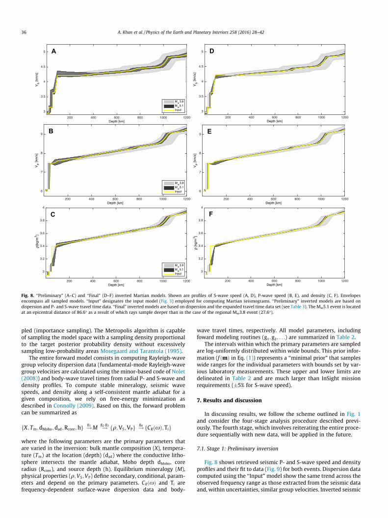
Fig. 8. ‘‘Preliminary” (A–C) and ‘‘Final” (D–F) inverted Martian models. Shown are profiles of S-wave speed (A, D), P-wave speed (B, E), and density (C, F). Envelopesencompass all sampled models. ‘‘Input” designates the input model (Fig. 3) employed for computing Martian seismograms. ‘‘Preliminary” inverted models are based ondispersion and P- and S-wave travel time data. ‘‘Final” inverted models are based on dispersion and the expanded travel time data set (see Table 3). The Mw5.1 event is locatedat an epicentral distance of 86.6� as a result of which rays sample deeper than in the case of the regional Mw3.8 event (27.6�).

36 A. Khan et al. / Physics of the Earth and Planetary Interiors 258 (2016) 28–42

pled (importance sampling). The Metropolis algorithm is capableof sampling the model space with a sampling density proportionalto the target posterior probability density without excessivelysampling low-probability areas Mosegaard and Tarantola (1995).

The entire forward model consists in computing Rayleigh-wavegroup velocity dispersion data (fundamental-mode Rayleigh-wavegroup velocities are calculated using the minor-based code of Nolet(2008)) and body-wave travel times from radial P- and S-wave anddensity profiles. To compute stable mineralogy, seismic wavespeeds, and density along a self-consistent mantle adiabat for agiven composition, we rely on free-energy minimization asdescribed in Connolly (2009). Based on this, the forward problemcan be summarized as

X; Tm;dMoho;dad;Rcore;hf g !g1 M !g2 ;g3 q;VS;VPf g !g4 CRðxÞ;Tif g

where the following parameters are the primary parameters thatare varied in the inversion: bulk mantle composition (X), tempera-ture (Tm) at the location (depth) (dad) where the conductive litho-sphere intersects the mantle adiabat, Moho depth dMoho, coreradius (Rcore), and source depth (h). Equilibrium mineralogy (M),physical properties (q;VS;VP) define secondary, conditional, param-eters and depend on the primary parameters. CRðxÞ and Ti arefrequency-dependent surface-wave dispersion data and body-

wave travel times, respectively. All model parameters, includingfoward modeling routines (g1; g2; . . .) are summarized in Table 2.

The intervals within which the primary parameters are sampledare log-uniformly distributed within wide bounds. This prior infor-mation (f ðmÞ in Eq. (1)) represents a ‘‘minimal prior” that sampleswide ranges for the individual parameters with bounds set by var-ious laboratory measurements. These upper and lower limits aredelineated in Table 2 and are much larger than InSight missionrequirements (�5% for S-wave speed).

7. Results and discussion

In discussing results, we follow the scheme outlined in Fig. 1and consider the four-stage analysis procedure described previ-ously. The fourth stage, which involves reiterating the entire proce-dure sequentially with new data, will be applied in the future.

7.1. Stage 1: Preliminary inversion

Fig. 8 shows retrieved seismic P- and S-wave speed and densityprofiles and their fit to data (Fig. 9) for both events. Dispersion datacomputed using the ‘‘Input” model show the same trend across theobserved frequency range as those extracted from the seismic dataand, within uncertainties, similar group velocities. Inverted seismic

15 20 25 30 35 40 452.5

2.55

2.6

2.65

2.7

2.75

Period [s]

Ray

leig

h−w

ave

grou

p ve

loci

ty [k

m/s

]

A

Mw3.8

−2 −1 0 1 20

0.3

P−wave travel time difference [s]

Pos

terio

r pr

obab

ility

−3 −2 −1 0 1 2 30

0.3

S−wave travel time difference [s]

B C

15 20 25 30 35 40 452.5

2.55

2.6

2.65

2.7

2.75

Period [s]

Ray

leig

h−w

ave

grou

p ve

loci

ty [k

m/s

] Mw5.1

D−2 −1 0 1 20

0.5

P−wave travel time difference [s]

Pos

terio

r pr

obab

ility

−3 −2 −1 0 1 2 30

0.25

S−wave travel time difference [s]

E F

Fig. 9. Comparison of observed and calculated data based on the inverted models shown in Fig. 8. (A, D) Calculated (gray lines) and observed Rayleigh-wave group velocities(circles) including uncertainties (error bars) and group velocities computed for the ‘‘Input” model shown in Fig. 3 (red circles). Travel time differences between computed andobserved P- (B, E) and S-wave arrivals (C, F). (For interpretation of the references to colour in this figure caption, the reader is referred to the web version of this article.)

20 30 40

Pro

babi

lity

h [km]27 27.5 28

Δ [°]−2 0 2

T0 [s]

A B C

Fig. 10. Re-located source parameters for the Mw3.8 event: (A) source depth (h); (B)epicentral distance (D); and (C) origin time (T0). For comparison, input sourceparameters are given in Table 1.

A. Khan et al. / Physics of the Earth and Planetary Interiors 258 (2016) 28–42 37

models are found to agree well with the ‘‘Input” model (comparewith yellow profile). Major features such as depth to Moho, abso-lute velocities, and densities are all captured in the inverted mod-els. Note that all models shown have large likelihood values, i.e., fitobservations within observational uncertainties (specified in Sec-tion 6). Differences between the inverted profiles for the twoevents are apparent in the relative widths of sampled models,which reflects the increased epicentral distance resulting in P-and S-waves that sample a much larger portion of the mantle thanis the case for the smaller regional event, in addition to dispersiondata that span a larger frequency range. From analysis of the pro-files, we find that the Rayleigh-wave dispersion data are mainlysensitive to S-wave speeds and that sensitivity extends to �200–250 km depth. To illustrate the simultaneous inversion for sourcelocation, inverted source parameters (epicentral distance, origintime, and source depth) for the Mw3.8 event are shown inFig. 10. These are found to be in good agreement with the inputparameters (c.f., Table 1). Interior structure and source locationwill be updated in the following through the addition of more data.

7.2. Stage 2: Iterative refinement – Identifying body-wave arrivals

Simultaneously with model inversion performed in stage 1, tra-vel times for a series of body-wave phases are computed for all

inverted models shown in Fig. 8. For this purpose we use the TauPtoolkit (Crotwell et al., 1999). The resultant travel time distribu-tions are employed as a means of identifying additional arrivalsthat would otherwise be difficult to assign and/or pick visually.This procedure is illustrated in Fig. 11, which shows the computedtravel time distributions for the various phases overlain directly onthe seismograms. Proceeding thus, we are able to identify a num-ber of additional phases such as sP and sS that help constrainsource depth, in addition to reflections from the surface (SS andSSS; see Fig. 4) and Moho (P^mP and SmS). Standard body-wavenomenclature and ray paths can be found at http://www.isc.ac.uk/standards/phases/. What we observe is that depending onwhich event is analyzed, some phases are easier to discriminatethan others, particularly those that relate to depth (pP, sP, and sS).As expected, depth phases are easier to identify in the case ofthe deep Mw3.8 event because these are well separated from theP- and S-wave arrivals unlike for the shallow Mw5.1 event. Wehave tried to pick phases as consistently as possible using the com-puted travel time distributions as primary guidance, but havenonetheless adjusted various picks according to personal judge-ment. This might possibly introduce inconsistencies, which couldbe offset by increasing the uncertainty on arrival time picks. Theadditional seismic phases thus identified for the two events aretabulated in Table 3.

We also computed travel-time distributions for typically verysmall-amplitude phases that are notoriously difficult to pick evenwith high-quality terrestrial seismic data. Picking core phasesPcP and ScS, which are of importance for estimating core radius,reliably from a single seismogram is difficult. These phases typi-cally only become visible after stacking of many seismograms. Thisis, however, unlikely to become a standard procedure in the con-text of InSight on Mars. Computed PcP and ScS travel time distribu-tions encompass the theoretically predicted PcP and ScS arrivals,but are too wide to allow us to unambiguously discriminate thecorrect arrival (Fig. 12). The large variations in computed PcP andScS travel times reflect the circumstance that inversion of

Mw5.1

A

Mw5.1

B

Mw3.8

C

Mw3.8

D

Fig. 11. Comparison of computed (vertical gray bars) and manually identified (vertical colored lines) body-wave arrivals for different seismic body-wave phases: plots A andB illustrate P- and S-wave phases for the Mw5.1 event and plots C and D show P- and S-wave phases for the Mw3.8 event. The distributions of computed travel times estimatedfrom the preliminary inverted models (Fig. 8) are shown as histograms (vertical gray bars) where probability of occurence scales with color: white(least probable)–black(most probable). Vertical yellow lines refer to travel times obtained from manual inspection of the seismograms used for the preliminary inversion and blue lines denote ourpicks once computed travel time distributions are available (see Table 3). Waveforms have been filtered (using a kausal Butterworth filer) in the period range 1–5 s (plots A, C,and D) and 1–20 s (plot B). Only vertical-component data are shown. Note that some phases such as the S-wave arrival for the Mw5.1 event have been picked on the horizontalcomponents (see Fig. 12). (For interpretation of the references to colour in this figure caption, the reader is referred to the web version of this article.)

38 A. Khan et al. / Physics of the Earth and Planetary Interiors 258 (2016) 28–42

surface-wave dispersion data and P- and S-wave arrivals are, asexpected, ill-suited to constrain core radius. Note that althoughPcP/ScS arrivals appear in some cases to overlap the direct P/S arri-vals, i.e., arrive prior to the latter, this is actually not the casebecause the corresponding P- and S-wave arrivals arrive earlierthan indicated by the yellow line in the figure. On a more specula-tive note, we envision that a core phase may possibly be pickedwith reasonable certainty so as to provide a useful first-order esti-

mate of core radius once several events have been analyzedsequentially, i.e., once a travel time database has been built up.

Finally, we should note that the identification of seismic arrivalsperformed here is not exhaustive; for the purpose of illustratingthe methodology we concentrated on the most obvious signalsand complex signal related to crustal reverberations (apparentfor the Mw5.1 event immediately after the first P- and S-wave arri-vals between �570–600 s and �1070–1150 s, respectively), for

Table 3Predicted and manually picked body-wave travel times, including pick uncertainty,for the seismic phases that could be identified initially (marked with ⁄) and afterpreliminary inversion. Predicted travel time refers to travel times computed from the‘‘Input” model shown in Fig. 3. Manually picked travel times are obtained from visualinspection of the synthetic seismograms. No picks were made for the core phases PcPand ScS because inversion based on dispersion data and P- and S-wave arrivals is notable to constrain lower mantle structure/core size (see Fig. 12).

Phase Predicted travel time (s) Picked travel time (s)

Source 1 (Mw5.1)P⁄ 556.9 556 � 1PcP 569.0 –P^mP 650.5 652.0 � 2PP 662.4 664.2 � 2PPP 689.3 694.0 � 2S⁄ 1044.4 1044.4 � 1ScS 1068.1 –S^mS 1200.8 1203.2 � 2SS 1225.4 1225.0 � 2

Source 2 (Mw3.8)P⁄ 217.4 216.9 � 1P^mP 221.3 221.0 � 1pP⁄ 223.3 223.9 � 2sP 229.1 229.5 � 2S⁄ 399.6 398.9 � 1sS 414.0 413.0 � 2SS 433.3 432.3 � 2SSS 465.8 465.4 � 2

A. Khan et al. / Physics of the Earth and Planetary Interiors 258 (2016) 28–42 39

example, is not considered. On a more general note, assigningphases can be challenging and while the use of travel time predic-tions based on ‘‘Preliminary” inverted models presents a promisingmeans for picking additional phases, assigning body-wave arrivalswill nonetheless depend crucially on the backgraound noise level.Thus, although mislabeling of seismic phases is potentially possi-ble, we expect that in a subsequent inversion the wrongly assignedphase can not be fit, as a result of which the potential outlier can beisolated and relabeled. This procedure summarizes iterative refine-ment, a central theme of the methodology proposed herein.

7.3. Stage 3: ‘‘Final” inversion

With the additional arrivals, the entire data set is reinverted fora new set of interior structure models and source parameters (epi-central distance and origin time). The ‘‘Final” models are shown inFig. 8. Comparison with ‘‘Preliminary” models shows, as expected,the additional gain in information obtained through inversion of

A

Fig. 12. Comparison of computed range of PcP (A) and ScS (B) arrival times (gray area)line) PcP arrival for model ‘‘Input” (Fig. 3). The vertical yellow line refers to the P- and S-inversion. Traces are filtered in the frequency range 1–5 s and show vertical (A) and horizthis figure caption, the reader is referred to the web version of this article.)

the expanded travel time data set. Proceeding in this manner, wecan iteratively improve our results as data become available bycontinuously building upon and refining previous models andevent locations (stage 4).

In summary, data-constrained pre-selection and refinement ofthe location of seismic phases presents a powerful complimentarymeans of obtaining additional information. In particular, as dataand events accumulate, continuous refinement and narrowing ofthe travel time and model parameter distributions will likely bethe means by which progress will be achieved. However, the feasi-bility of the present approach will depend strongly on the nature ofthe data and sources that will be recorded, including installationcharacteristics, level of background seismic noise on Mars, andMartian seismicity.

8. Conclusion and summary remarks

In this study, we have described a methodology that, based on arepresentative set of 3-component seismograms from singleevents, (1) determines location, origin time, and back azimuth ofmarsquakes probabilistically using surface- and body-wave traveltime information, in addition to P-wave and surface-wave polar-ization; (2) extracts information on surface-wave dispersion char-acteristics and inverts this information in combination with body-wave travel times for 1D models of interior structure; (3) employsthe inverted models to produce travel time distributions of addi-tional body wave phases as an aid in picking arrivals where iden-tification is otherwise difficult or unfavorable; (4) reinverts theexpanded data set for a new set of interior structure models andsource parameters; and (5) iteratively refines and updates modelsand source locations by continued analysis of new events.

In the absence of Martian seismic data, we computed syntheticseismograms down to a period of 1 s using full waveform tech-niques based on the axisymmetric spectral element method Axi-SEM. Models for the interior of Mars (radial profiles of density, P-and S-wave-speed, and attenuation) have been constructed onthe basis of an average Martian mantle composition and modelareotherm using thermodynamic principles and mineral physicsdata and were used to create synthetic waveforms. Noise wasadded to the synthetic seismograms in order to mimic the condi-tions that we envisage with the data returned from the seismome-ter deployed by the Mars InSight lander. This noise is based on thecurrently most realistic noise model that considers many possiblesources. In order to demonstrate the methodology, we considered

B

for all ‘‘Preliminary” inverted models with the theoretically predicted (vertical bluewave arrival obtained by manual inspection of the seismogram in the ‘‘Preliminary”ontal (B) components, respectively. (For interpretation of the references to colour in

40 A. Khan et al. / Physics of the Earth and Planetary Interiors 258 (2016) 28–42

sources similar to those contained in a realistic Martian seismicitycatalogue. These include a relatively large-sized event (Mw5.1) atan epicentral distance of 86.6� for which both major- and minor-arc surface waves (R1, R2, and R3) and body wave arrivals areavailable and a smaller event (Mw3.8) at a distance of 27.6� forwhich only the minor-arc surface wave (R1) and body wave arri-vals are usable.

Applying our location algorithm (Böse et al., 2016) on the syn-thetic waveforms, we have shown that we are able to locate anevent in space (epicentral distance, back azimuth, and sourcedepth) and time to high accuracy. Epicentral distance and origintime were determined to an accuracy of �0.5–1� and �3–6 s,respectively, whereas source depth could be determined to anaccuracy of 1–2 km (for those events where seismic depth phasescould be identified). With the particular events and noise level cho-sen, we were able to extract information on Rayleigh-wave groupvelocity dispersion in the period ranges 14–48 s (Mw5.1) and 14–34 s (Mw3.8), respectively. Inversion of the dispersion data in com-bination with body-wave travel time picks allows us to determinemantle velocity structure to an uncertainty of 65% for VS and �5%for VP.

This study is based on purely radial models and complexitiesrelated to three-dimensional structure, particularly in the crustand lithosphere, will undoubtedly render the waveforms morecomplex than envisaged here. As discussed in more detail in Böseet al. (2016), we foresee the following complexities arise: (1) scat-tering - broadening of surface wave-train and decreased ampli-tudes at short periods; (2) crustal dichotomy – modification ofRayleigh-wave travel time; (3) Mars’ ellipticity - change in traveltime of Rayleigh-waves relative to a spherically symmetric model,as a result of which estimates of epicentral distance and origintime will be affected. The full extent to which these effects inter-fere with the present approach are currently being investigatedand will be described in forthcoming analyses. However, sincecrustal thickness is known to within a constant factor (Neumannet al., 2004; Wieczorek and Zuber, 2004), including ellipticity cor-rections commonly applied in surface-wave tomography on Earth(Nolet, 2008) are expected to be applicable on Mars.

In spite of such caveats, we have demonstrated the feasibility ofour single-station-single-event surface-wave-based procedure forlocating marsquakes, extracting and inverting dispersion data incombination with body-wave travel times. Following this, we haveshown how the inverted models can be used as a diagnostic tool toaid in locating seismic phases that might elude visual identificationor otherwise be difficult to assign. While the identification of seis-mic phases performed here was limited to the most distinct arri-vals and served to illustrate the predictive power of the method,we envision improved analysis in the future by combining withpolarization and amplitude information.

In the future we will also consider aspects of interior structureinterpretation. As an example, we may note the importance of alow-velocity layer in the upper mantle of Mars. If present, such alayer provides insights into the dynamics of the Martian mantle,its volatile content, and thermal evolution. The seismic signatureof a low-velocity layer is distinct from that produced by modelswithout this feature, making it potentially observable with a singleseismic station (Okal and Anderson, 1978; Zheng et al., 2015). Asdiscussed by Zheng et al. (2015), the most obvious candidates fordetecting a low-velocity layer are direct body-wave arrivals (P orS), through the presence of a shadow zone and the dispersion char-acteristics of surface-waves. Detecting a shadow zone with a singlestation will nonetheless remain challenging and will depend criti-cally on Martian seismic activity and the geographical distributionof marsquakes. In comparison, if relatively large surface-waves areexcited, these will, by the methodology employed herein, provide arelatively easy tool for distinguishing models with and without

low-velocity layers through the characteristic form of the disper-sion curve that these give rise to. Note that this can be done with-out knowledge of the location of the particular marsquake. Inrelation hereto, excitation of normal modes by a sufficiently largemarsquake such as the one modeled in this study, will providean independent means of inverting for structure (Lognonné et al.,1996).

Ultimately, the success of the methodology developed here forlocating marsquakes and determining structural parameters, willdepend crucially on the as yet unknown levels of Martian seismic-ity and background noise. Extracting longer period surface waves,including Love waves in addition to Rayleigh waves as well asovertones, would help in sounding deeper into the mantle, but,again, will hinge on the level of background seismic noise on Mars,installation characteristics, and Martian seismicity. These parame-ters will be estimated with the return of data beginning November2018.

Acknowledgements

We would like to thank Lapo Boschi and an anonymousreviewer for comments on the manuscript. We would also like toacknowledge Francis Nimmo for sharing his visco-elastic attenua-tion code. This work was supported by grants from the SwissNational Science Foundation (SNF-ANR project 157133 ‘‘Seismol-ogy on Mars”) and from the Swiss National Supercomputing Centre(CSCS) under project ID s528. Numerical computations have alsobeen performed on the ETH cluster Brutus.

Appendix A. Supplementary data

Supplementary data associated with this article can be found, inthe online version, at http://dx.doi.org/10.1016/j.pepi.2016.05.017.

References

Al-Attar, D., Woodhouse, J.H., 2008. Calculation of seismic displacement fields inself-gravitating earth models–applications of minors vectors and symplecticstructure. Geophys. J. Int. 175 (3), 1176–1208.

Anderson, D.L., 1989. Theory of the Earth. Blackwell Scientific Publications.Anderson, D.L., Given, J.W., 1982. Absorption band q model for the earth. J. Geophys.

Res. Solid Earth 87 (B5), 3893–3904.Anderson, D.L., Miller, W.F., Latham, G.V., Nakamura, Y., Toksoz, M.N., Dainty, A.M.,

Duennebier, F.K., Lazarewicz, A.R., Kovach, R.L., Knight, T.C.D., 1977. Seismologyon Mars. J. Geophys. Res. 82, 4524–4546.

Banerdt, W.B., Smrekar, S., Lognonné, P., Spohn, T., Asmar, S.W., Banfield, D., Boschi,L., Christensen, U., Dehant, V., Folkner, W., Giardini, D., Goetze, W., Golombek,M., Grott, M., Hudson, T., Johnson, C., Kargl, G., Kobayashi, N., Maki, J., Mimoun,D., Mocquet, A., Morgan, P., Panning, M., Pike, W.T., Tromp, J., van Zoest, T.,Weber, R., Wieczorek, M.A., Garcia, R., Hurst, K., Mar. 2013. InSight: A DiscoveryMission to Explore the Interior of Mars. In: Lunar and Planetary ScienceConference. Vol. 44 of Lunar and Planetary Inst. Technical Report. p. 1915.

Benjamin, D., Wahr, J., Ray, R.D., Egbert, G.D., Desai, S.D., 2006. Constraints onmantle anelasticity from geodetic observations, and implications for the J2anomaly. Geophys. J. Int. 165, 3–16.

Bertka, C.M., Fei, Y., 1997. Mineralogy of the Martian interior up to core-mantleboundary pressures. J. Geophys. Res. 102, 5251–5264.

Bertka, C.M., Fei, Y., 1998. Density profile of an SNC model Martian interior and themoment-of-inertia factor of Mars. Earth Planet. Sci. Lett. 157, 79–88.

Bills, B.G., Neumann, G.A., Smith, D.E., Zuber, M.T., 2005. Improved estimate of tidaldissipation within Mars from MOLA observations of the shadow of Phobos. J.Geophys. Res. (Planets) 110, 7004.

Böse, M., Clinton, J., Ceylan, S., Euchner, F., van Driel, M., Khan, A., Giardini, D., 2016.A Probabilistic framework for single-station location of seismicity on Earth andMars. Phys. Earth Planet Sci. in preparation.

Chael, E.P., 1997. An automated rayleigh-wave detection algorithm. Bull. Seismol.Soc. Am. 87 (1), 157–163.

Connolly, J.A.D., 2009. The geodynamic equation of state: what and how. Geochem.Geophys. Geosyst. 10 (10), n/a–n/a, q1001.

Crotwell, H.P., Owens, T.J., Ritsema, J., 1999. The taup toolkit: flexible seismic travel-time and ray-path utilities. Seismol. Res. Lett. 70 (2), 154–160.

Dreibus, G., Wänke, H., 1985. Mars, a volatile-rich planet. Meteoritics 20, 367–381.Durek, J.J., Ekström, G., 1996. A radial model of anelasticity consistent with long-

period surface-wave attenuation. Bull. Seismol. Soc. Am. 86 (1A), 144–158.

A. Khan et al. / Physics of the Earth and Planetary Interiors 258 (2016) 28–42 41

Dziewonski, A., Romanowicz, B., 2007. 1.01 – overview. In: Schubert, G. (Ed.),Treatise on Geophysics. Elsevier, Amsterdam, pp. 1–29.

Dziewonski, A.M., Anderson, D.L., 1981. Preliminary reference Earth model. Phys.Earth Planet. Inter. 25, 297–356.

Efroimsky, M., 2012. Tidal dissipation compared to seismic dissipation: in smallbodies, Earths, and super-earths. Astrophys. J. 746, 150.

Eisermann, A.S., Ziv, A., Wust-Bloch, G.H., 2015. Real-time Back Azimuth forEarthquake Early Warning. Bulletin of the Seismological Society of America.

Gagnepain-Beyneix, J., Lognonné, P., Chenet, H., Lombardi, D., Spohn, T., 2006. Aseismic model of the lunar mantle and constraints on temperature andmineralogy. Phys. Earth Planet. Inter. 159, 140–166.

Garcia, R.F., Gagnepain-Beyneix, J., Chevrot, S., Lognonné, P., 2011. Very preliminaryreference Moon model. Phys. Earth Planet. Inter. 188, 96–113.

Golombek, M.P., Banerdt, W.B., Tanaka, K.L., Tralli, D.M., 1992. A prediction of Marsseismicity from surface faulting. Science 258, 979–981.

Grimm, R.E., 2013. Geophysical constraints on the lunar Procellarum KREEPTerrane. J. Geophys. Res. (Planets) 118, 768–778.

Gudkova, T.V., Lognonné, P., Gagnepain-Beyneix, J., 2011. Large impacts detected bythe Apollo seismometers: impactor mass and source cutoff frequencyestimations. Icarus 211, 1049–1065.

Jackson, I., Faul, U.H., 2010. Grainsize-sensitive viscoelastic relaxation in olivine:towards a robust laboratory-based model for seismological application. Phys.Earth Planet. Inter. 183, 151–163.

Karato, S.-i., 2013. Geophysical constraints on the water content of the lunar mantleand its implications for the origin of the Moon. Earth Planet. Sci. Lett. 384, 144–153.

Kawamura, T., Kobayashi, N., Tanaka, S., Lognonné, P., 2015. Lunar SurfaceGravimeter as a lunar seismometer: investigation of a new source of seismicinformation on the Moon. J. Geophys. Res. (Planets) 120, 343–358.

Khan, A., Connolly, J.A.D., 2008. Constraining the composition and thermal state ofMars from inversion of geophysical data. J. Geophys. Res. (Planets) 113, 7003.

Khan, A., Connolly, J.A.D., Pommier, A., Noir, J., 2014. Geophysical evidence for meltin the deep lunar interior and implications for lunar evolution. J. Geophys. Res.(Planets) 119, 2197–2221.

Khan, A., Mosegaard, K., 2002. An inquiry into the lunar interior: a nonlinearinversion of the Apollo lunar seismic data. J. Geophys. Res. (Planets) 107, 5036.

Khan, A., Mosegaard, K., Williams, J.G., Lognonné, P., 2004. Does the Moon possess amolten core? Probing the deep lunar interior using results from LLR and LunarProspector. J. Geophys. Res. (Planets) 109, 9007.

Khan, A., Pommier, A., Neumann, G., Mosegaard, K., 2013. The lunar moho and theinternal structure of the moon: a geophysical perspective. Tectonophysics 609,331–352, moho: 100 years after Andrija Mohorovicic.

Knapmeyer, M., 2004. Ttbox: a matlab toolbox for the computation of 1dteleseismic travel times. Seismol. Res. Lett. 75 (6), 726–733.

Knapmeyer, M., Oberst, J., Hauber, E., Wählisch, M., Deuchler, C., Wagner, R., 2006.Working models for spatial distribution and level of Mars’ seismicity. J.Geophys. Res. E Planets 111 (11), 1–23.

Knapmeyer, M., Weber, R.C., 2015. Seismicity and interior structure of the moon. In:Tong, V.C.H., Garcia, R.A. (Eds.), Extraterrestrial Seismology. CambridgeUniversity Press, Cambridge, pp. 203–225.

Kuskov, O.L., Panferov, A.B., 1993. Thermodynamic models for the structure of themartian upper mantle. Geochem. Int. 30, 132.

Lainey, V., Dehant, V., Pätzold, M., 2007. First numerical ephemerides of the Martianmoons. Astron. Astrophys. 465, 1075–1084.

Larmat, C., Montagner, J.-P., Capdeville, Y., Banerdt, W.B., Lognonné, P., Vilotte, J.-P.,2008. Numerical assessment of the effects of topography and crustal thicknesson martian seismograms using a coupled modal solution spectral elementmethod. Icarus 196, 78–89.

Lognonné, P., Banerdt, W.B., Giardini, D., Christensen, U., Mimoun, D., de Raucourt,S., Spiga, A., Garcia, R., Mocquet, A., Panning, M., Beucler, E., Boschi, L., Goetz, W.,Pike, T., Johnson, C., Weber, R., Wieczorek, M., Larmat, K., Kobayashi, N., Tromp,J., Mar. 2012. Insight and single-station broadband seismology: from signal andnoise to interior structure determination. In: Lunar and Planetary ScienceConference. vol. 43 of Lunar and Planetary Inst. Technical Report. p. 1983.

Lognonné, P., Beyneix, J.G., Banerdt, W.B., Cacho, S., Karczewski, J.F., Morand, M.,1996. Ultra broad band seismology on InterMarsNet. Planets Space Sci. 44,1237.

Lognonné, P., Gagnepain-Beyneix, J., Chenet, H., 2003. A new seismic model of theMoon: implications for structure, thermal evolution and formation of the Moon.Earth Planet. Sci. Lett. 211, 27–44.

Lognonné, P., Johnson, C., 2007. 10.03 – planetary seismology. In: Schubert, G. (Ed.),Treatise on Geophysics. Elsevier, Amsterdam, pp. 69–122.

Lognonné, P., Mosser, B., 1993. Planetary seismology. Surv. Geophys. 14, 239–302.Lognonné, P., Pike, T.W., 2015. Planetary seismometry. In: Tong, V.C.H., Garcia, R.A.

(Eds.), Extraterrestrial Seismology. Cambridge University Press, Cambridge, pp.91–106.

Longhi, J., Knittle, E., Holloway, J.R., Wänke, H., 1992. The bulk composition,mineralogy and internal structure of Mars. In: Kieffer, H.H., Jakosky, B.M.,Snyder, C.W., Matthews, M.S. (Eds.). Mars. Univ of Arizona Press, pp. 184–208.

Lyubetskaya, T., Korenaga, J., 2007. Chemical composition of earth’s primitivemantle and its variance: 1. method and results. J. Geophys. Res. Solid Earth 112(B3), n/a–n/a, b0321.

McDonough, W.s., Sun, S., 1995. The composition of the earth. Chem. Geol. 120 (34),223–253, chemical Evolution of the Mantle.

McSween Jr., H.Y., 1994. What we have learned about Mars from SNC meteorites.Meteoritics 29, 757–779.

Mimoun, D., Lognonné, P., Banerdt, W.B., Hurst, K., Deraucourt, S., Gagnepain-Beyneix, J., Pike, T., Calcutt, S., Bierwirth, M., Roll, R., Zweifel, P., Mance, D.,Robert, O., Nébut, T., Tillier, S., Laudet, P., Kerjean, L., Perez, R., Giardini, D.,Christenssen, U., Garcia, R., Mar. 2012. The InSight SEIS experiment. In: Lunarand Planetary Science Conference. vol. 43 of Lunar and Planetary Inst. TechnicalReport. p. 1493.

Minster, J.B., Anderson, D.L., 1981. A model of dislocation-controlled rheology forthe mantle. R. Soc. 299 (1449), 319–356.

Mocquet, A., Vacher, P., Grasset, O., Sotin, C., 1996. Theoretical seismic models ofMars: the importance of the iron content of the mantle. Planets Space Sci. 44,1251–1268.

Mosegaard, K., Tarantola, A., 1995. Monte carlo sampling of solutions to inverseproblems. J. Geophys. Res.: Solid Earth (1978–2012) 100 (B7), 12431–12447.

Murdoch, M., Minoun, D., Lognonné, P.H., SEIS science team, 2015a. Seisperformance model environment document. Tech. rep., ISGH-SEIS-JF-ISAE-030.

Murdoch, M., Minoun, D., Lognonné, P.H., SEIS science team, 2015b. Seisperformance budgets. Tech. rep., ISGH-SEIS-JF-ISAE-0010.

Nakamura, Y., 1983. Seismic velocity structure of the lunar mantle. J. Geophys. Res.88, 677–686.

Nakamura, Y., 2015. Planetary seismology: early observational results. In: Tong, V.C.H., Garcia, R.A. (Eds.), Extraterrestrial Seismology. Cambridge University Press,Cambridge, pp. 91–106.

Neumann, G.A., Zuber, M.T., Wieczorek, M.A., McGovern, P.J., Lemoine, F.G., Smith,D.E., 2004. Crustal structure of mars from gravity and topography. J. Geophys.Res.: Planets 109 (E8), e08002.

Nimmo, F., Faul, U.H., 2013. Dissipation at tidal and seismic frequencies in a melt-free, anhydrous Mars. J. Geophys. Res. (Planets) 118, 2558–2569.

Nimmo, F., Faul, U.H., Garnero, E.J., 2012. Dissipation at tidal and seismicfrequencies in a melt-free Moon. J. Geophys. Res. (Planets) 117, 9005.

Nissen-Meyer, T., van Driel, M., Stähler, S.C., Hosseini, K., Hempel, S., Auer, L.,Colombi, A., Fournier, A., 2014. AxiSEM: broadband 3-D seismic wavefields inaxisymmetric media. Solid Earth 5 (1), 425–445.

Nolet, G., 2008. A Breviary of Seismic Tomography. Cambridge University Press,Cambridge, UK.

Okal, E.A., Anderson, D.L., 1978. Theoretical models for Mars and their seismicproperties. Icarus 33, 514–528.

Panning, M.P., Beucler, É., Drilleau, M., Mocquet, A., Lognonné, P., Banerdt, W.B.,2015. Verifying single-station seismic approaches using Earth-based data:preparation for data return from the InSight mission to Mars. Icarus 248, 230–242.

Peterson, J., 1993. Observations and modeling of seismic background noise. Tech.Rep. Open–File Report 93–322, US Geological Survey, Alburquerque, NewMexico.

Phillips, R., 1991. Expected rate of marsquakes. In: Scientific Rationale andRequirements for a Global Seismic Network on Mars. vol. 91-02, LPI TechnicalRep. Lunar and Planetary Institute, Houston TX, pp. 35–38.

Pommier, A., Leinenweber, K., Tasaka, M., 2015. Experimental investigation of theelectrical behavior of olivine during partial melting under pressure andapplication to the lunar mantle. Earth Planet. Sci. Lett. 425, 242–255.

Rivoldini, A., Van Hoolst, T., Verhoeven, O., Mocquet, A., Dehant, V., 2011. Geodesyconstraints on the interior structure and composition of Mars. Icarus 213, 451–472.

Selby, N.D., 2001. Association of rayleigh waves using backazimuth measurements:application to test ban verification. Bull. Seismol. Soc. Am. 91 (3), 580–593.

Smith, D.E., Zuber, M.T., Mar. 2002. The crustal thickness of mars: accuracy andresolution. In: Lunar and Planetary Science Conference. vol. 33 of Lunar andPlanetary Inst. Technical Report. p. 1893.

Sohl, F., Schubert, G., Spohn, T., 2005. Geophysical constraints on the compositionand structure of the Martian interior. J. Geophys. Res. (Planets) 110, 12008.

Stixrude, L., Lithgow-Bertelloni, C., 2005a. Thermodynamics of mantle minerals – I.Physical properties. Geophys. J. Int. 162, 610–632.

Stixrude, L., Lithgow-Bertelloni, C., 2011. Thermodynamics of mantle minerals – II.Phase equilibria. Geophys. J. Int. 184, 1180–1213.

Taylor, G.J., 2013. The bulk composition of Mars. Chem. Erde/ Geochem. 73, 401–420.

Teanby, N.A., Wookey, J., 2011. Seismic detection of meteorite impacts on Mars.Phys. Earth Planet. Inter. 186, 70–80.

Treiman, A.H., 1986. The parental magma of the Nakhla achondrite: ultrabasicvolcanism on the shergottite parent body. Geochim. Cosmochim. Acta 50, 1061–1070.

van Driel, M., Krischer, L., Stähler, S.C., Hosseini, K., Nissen-Meyer, T., 2015.Instaseis: instant global seismograms based on a broadband waveformdatabase. Solid Earth 6 (2), 701–717.

Van Hoolst, T., Dehant, V., Roosbeek, F., Lognonné, P., 2003. Tidally induced surfacedisplacements, external potential variations, and gravity variations on Mars.Icarus 161, 281–296.

Verhoeven, O., Rivoldini, A., Vacher, P., Mocquet, A., Choblet, G., Menvielle, M.,Dehant, V., Van Hoolst, T., Sleewaegen, J., Barriot, J.-P., Lognonné, P., 2005.Interior structure of terrestrial planets: modeling Mars’ mantle and itselectromagnetic, geodetic, and seismic properties. J. Geophys. Res. (Planets)110, 4009.

Wang, Y., Wen, L., Weidner, D.J., 2013. Composition of Mars constrained usinggeophysical observations and mineral physics modeling. Phys. Earth Planet.Inter. 224, 68–76.

Weber, R.C., Lin, P.-Y., Garnero, E.J., Williams, Q., Lognonné, P., 2011. Seismicdetection of the lunar core. Science 331, 309.

42 A. Khan et al. / Physics of the Earth and Planetary Interiors 258 (2016) 28–42

Wieczorek, M.A., Zuber, M.T., 2004. Thickness of the martian crust: improvedconstraints from geoid-to-topography ratios. J. Geophys. Res.: Planets 109 (E1),e01009.

Williams, J.G., Boggs, D.H., 2015. Tides on the Moon: theory and determination ofdissipation. J. Geophys. Res. (Planets) 120, 689–724.

Williams, J.G., Boggs, D.H., Yoder, C.F., Ratcliff, J.T., Dickey, J.O., 2001. Lunarrotational dissipation in solid body and molten core. J. Geophys. Res. 106,27933–27968.

Yamada, R., Garcia, R.F., Lognonné, P., Kobayashi, N., Takeuchi, N., Nébut, T.,Shiraishi, H., Calvet, M., Ganepain-Beyneix, J., 2013. On the possibility of lunarcore phase detection using new seismometers for soft-landers in future lunarmissions. Planet. Space Sci. 81, 18–31.

Yamada, R., Matsumoto, K., Kikuchi, F., Sasaki, S., 2014. Error determination of lunarinterior structure by lunar geodetic data on seismic restriction. Phys. EarthPlanet. Inter. 231, 56–64.

Yoder, C.F., Konopliv, A.S., Yuan, D.N., Standish, E.M., Folkner, W.M., 2003. Fluid coresize of mars from detection of the solar tide. Science 300, 299–303.

Zharkov, V.N., Gudkova, T.V., 1997. On the dissipative factor of the Martian interiors.Planets Space Sci. 45, 401–407.

Zharkov, V.N., Gudkova, T.V., 2005. Construction of Martian interior model. Sol. Syst.Res. 39, 343–373.

Zheng, Y., Nimmo, F., Lay, T., 2015. Seismological implications of a lithospheric lowseismic velocity zone in mars. Phys. Earth Planet. Inter. 240, 132–141.