SINGLE-PHASE INDUCTION - NASA of single-phase induction pumps is largely dependent on two dimension- less quantities, flow magnetic Reynolds number and frequency magnetic Reynolds

.r . . ., L

I

I

N A

0 QI m

S A

.I - . '

TECHNICAL NOTE

d

u L.

ICATEKORY) I (NASA CR OR TMX OR AD NUMBER)

SINGLE-PHASE INDUCTION ELECTROMAGNETIC PUMP

by Richard E. Scbwirian Lewis Researcb Center Cleveland, Ohio

N AT

NASA TN D-3950

O N A L A E R O N A U T I C S A N D SPACE A D M I N I S T R A T I O N W A S H I N G T O N , D. C. M A Y 1967

https://ntrs.nasa.gov/search.jsp?R=19670015148 2018-05-30T22:12:12+00:00Z

NASA TN D-3950

SINGLE-PHASE INDUCTION ELECTROMAGNETIC PUMP

By Richa rd E . Schwir ian I

! Lewis R e s e a r c h C e n t e r Cleveland, Ohio

NATIONAL AERONAUT ICs AND SPACE ADMlN I STRATI ON ~~

For sale by the Clearinghouse for Federal Scientific and Technical Information Springfield, Virginia 22151 - CFSTI price $3.00

SINGLE-PHASE IN DUCTION ELECTROMAGNETIC PUMP

c

by Richard E. S c h w i r i a n

Lewis Research Center

SUMMARY k

Analyses of two single-phase induction electromagnetic pumps in which induced elec- t r ical currents flow circumferentially in an annulus are presented. The analysis as- sumes a purely radial magnetic field, and differential equations describing the dependence of the magnetic field on the axial coordinate are obtained by using the integrated form of Ampere's law, Maxwell's equations, and Ohm's law. General solutions to these equations are obtained and are applied to specific configurations by assigning the appropriate boundary conditions at the annulus inlet and outlet.

Performance of single-phase induction pumps is largely dependent on two dimensionless quantities, flow magnetic Reynolds number and frequency magnetic Reynolds number. Dimensionless functions of these magnetic Reynolds numbers a r e developed from which calculations of developed pressure, efficiency, core magnetic field strength, and current-voltage requirements can be made. Calculations of efficiency and dimensionless developed pressure are also made. It is shown that, for the cases of low flow magnetic Reynolds number with low frequency magnetic Reynolds number and high flow magnetic Reynolds number with low frequency magnetic Reynolds number, simple expressions for ideal efficiency can be obtained.

Finally, a comparison of these single-phase induction pump designs with traveling- field induction pumps of similar geometry is made. For the particular application considered, the efficiency differences between single-phase and traveling-field pumps are negligible. traveling-field pumps at high temperatures and are, therefore, more adaptable to space

Furthermore, single-phase pumps are potentially more reliable than

~' power systems.

INTRODUCTION

In space electric power systems using the liquid alkali metals either as a working fluid o r as a heat-transfer medium, a need exists for pumping units of high reliability,

low weight, and high efficiency. For such systems, both the impeller-type pump and the electromagnetic pump are being considered. 4

To date, attention has been focused primarily on the canned motor-driven impeller pump for space application because of its somewhat higher predicted efficiency and lower predicted weight as compared with conventional electromagnetic pumps. Recent studies (ref. l), however, indicate that, for space applications, electromagnetic pumping Sys- tems having weights comparable to motor-driven impeller pumping systems can be designed. Furthermore, the reliability gained by eliminating the necessity of bearings and seals and all other moving par ts makes the electromagnetic pump quite attractive.

temperature space power systems is the single-phase induction pump. Induction electromagnetic pumps generally are more reliable than conduction electromagnetic pumps because of the lack of electrodes, thereby eliminating the mechanically difficult electrode- duct connections. As opposed to the only other induction pump (the traveling-field de- vice), the single-phase pump has an advantage in that the exciting coils need not be placed in close proximity to the hot fluid. Coil electrical insulation problems are therefore simplified, and coil electrical 1c;sses are decreased because of the reduced coil temperature. Because of this advantage, the single-phase pump should be more adaptable to high-temperature applications than conduction o r traveling-f ield pumps.

the unsteady nature of the developed pressure (see ref. 1). Even though the maximum obtainable ideal efficiency of single-phase pumps is less than the maximum obtainable ideal efficiency of traveling-field pumps, real efficiencies could be comparable o r greater. The reasons for this are twofold: First, lower coil losses are made possible by a lower coil temperature. Second, for a required number of excitation ampere turns, the coil losses can be further reduced by increasing the coil size and, therefore, de- creasing the current density. This is done, however, at the expense of increased pump weight.

considered the magnetic-field distortion created when an alternating, transverse magnetic field is impressed on a conducting fluid flowing axially in an annular duct. Appro- priate boundary conditions are applied and curves of magnetic field strength against axial distance a r e presented. Fthudy (ref. 1) extended Watt's work to include approximate corrections f o r the effects of nonzero duct-wall conductivity and also presented equations that could be used for computing output pressure and both fluid and duct -wall electrical losses. Rhudy also suggested another single-phase pump configuration that required less magnetic material than Watt ' s configuration but was less efficient. In neither of these papers were general performance characterist ics of single-phase pumps discussed o r general curves of performance presented.

The most potentially reliable of all electromagnetic pumps fo r application in high-

Disadvantages of the single-phase pump are its low ideal efficiency, high weight, and

The single-phase pump was first conceived by Watt (ref. 2). In his report, Watt

2

II

The purpose of this report is to make an analysis of two single-phase induction 4 pumps and to obtain general performance curves from which the parameters that will op-

timize the performance of such pumps can be determined. Performance is shown to depend largely on the two dimensionless quantities, flow magnetic Reynolds number and frequency magnetic Reynolds number, where magnetic Reynolds number is defined as the dimensionless product of a characteristic permeability, electrical conductivity, velocity, and length of the system. Curves of ideal efficiency, dimensionless ideal pressure, and dimensionless core magnetic field strength a r e given as functions of these two magnetic Reynolds numbers for two types of the single-phase pump. Other dimensionless functions that can be used to compute nonideal performance and current-voltage requirements are also presented, and trends at low values of flow and frequency magnetic Reynolds numbers a r e discussed. Finally, comparisons of performance with that of annular traveling-field pump, which is geometrically quite similar to the single-phase pump under consideration, a r e made, and conclusions are reached concerning efficiency, reliability, and weight.

~ '

,

ANALY S I S

S i ngle-P hase Pump Concept

The body force in many electromagnetic pumps, including the single-phase pump, can be consickred as resulting from a magnetic pressure gradient. This concept wi!! be quite convenient in understanding single -phase pump operation.

The equations governing the distribution and magnitude of the electric and magnetic fields E and B in an isotropic, charge-free medium, are, when displacement current t e rms are neglected,

e 4

0

V X E = - - (Faraday's law) a t

e 4

V x B = p j (Ampere's law)

v . g = o

v . E = o (3)

(4)

(5) 0

j = o(2 + V'X E) (Ohm's law)

(Symbols are defined in appendix A. )

must be satisfied. If a complete analytical solution for electric field strength E and For any system to which the aforementioned assumptions apply, equations * (1) to (5)

3

-c 4

magnetic field strength B is obtainable, then current density j can be computed ac- cording to Ohm’s law (ea_. (5)) o r Ampere’s law (eq. (2)) F n r cond-~ctinn and traveling- field electromagnetic pumps, electrical current can conveniently be thought of as arising from the presence, in a medium of electrical conductivity u, of a field + q X B‘. This point of view is suggested by Ohm’s law. A less common but equally valid point of view is to consider electrical current as a manifestation of a distorted magnetic fieid. This latter point of view is most helpful in understanding the principle of operation of the single-phase induction pump.

Consider the situation depicted in figure 1(b) in which a conducting fluid flows with velocity v‘ through a magnetic field of finite extent in the z-direction. If the magnetic field strength B‘ is assumed to have a component in the y-direction only and if the y- and x-derivatives are neglected, equations (2) and (5) imply that

*

Solving equation (6) gives

povz B = C o e Y

If a certain amount of magnetic flux <pm must pass through the fluid, then the appropriate boundary condition is

C qrn = ,( Coepuvz dz

for a unit width in x-direction. Equation (8) determines the constant Co:

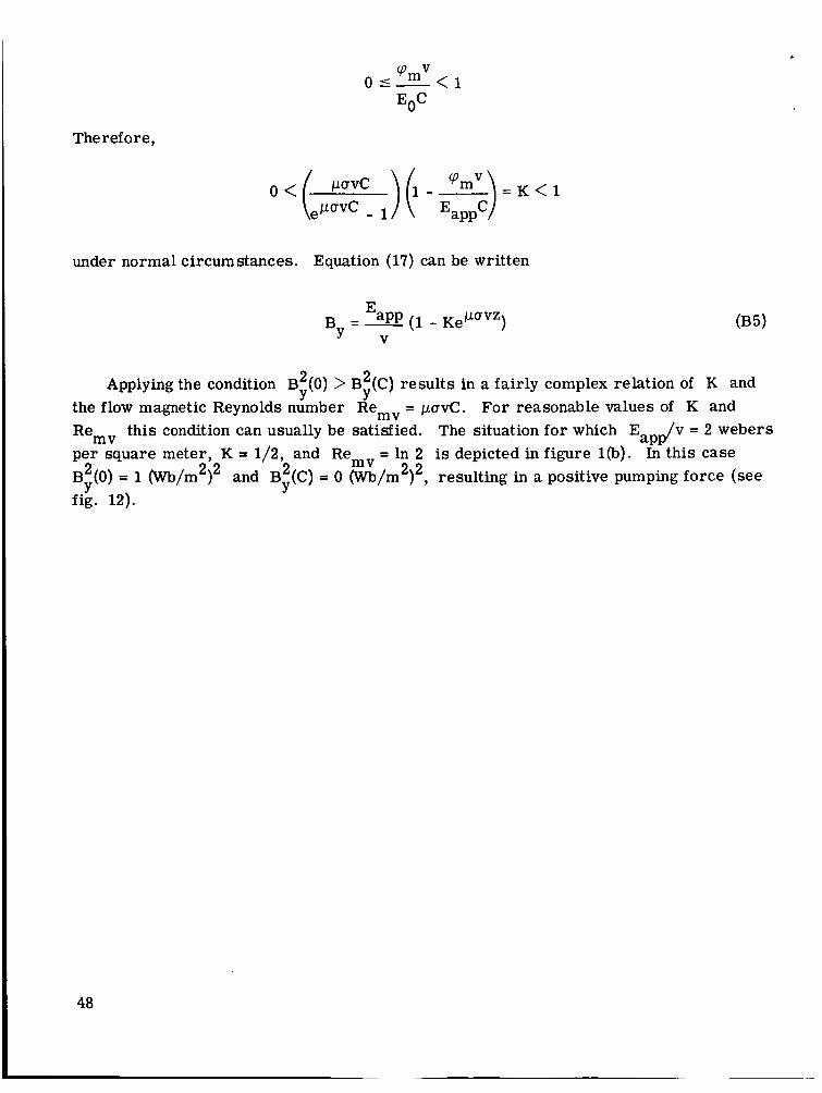
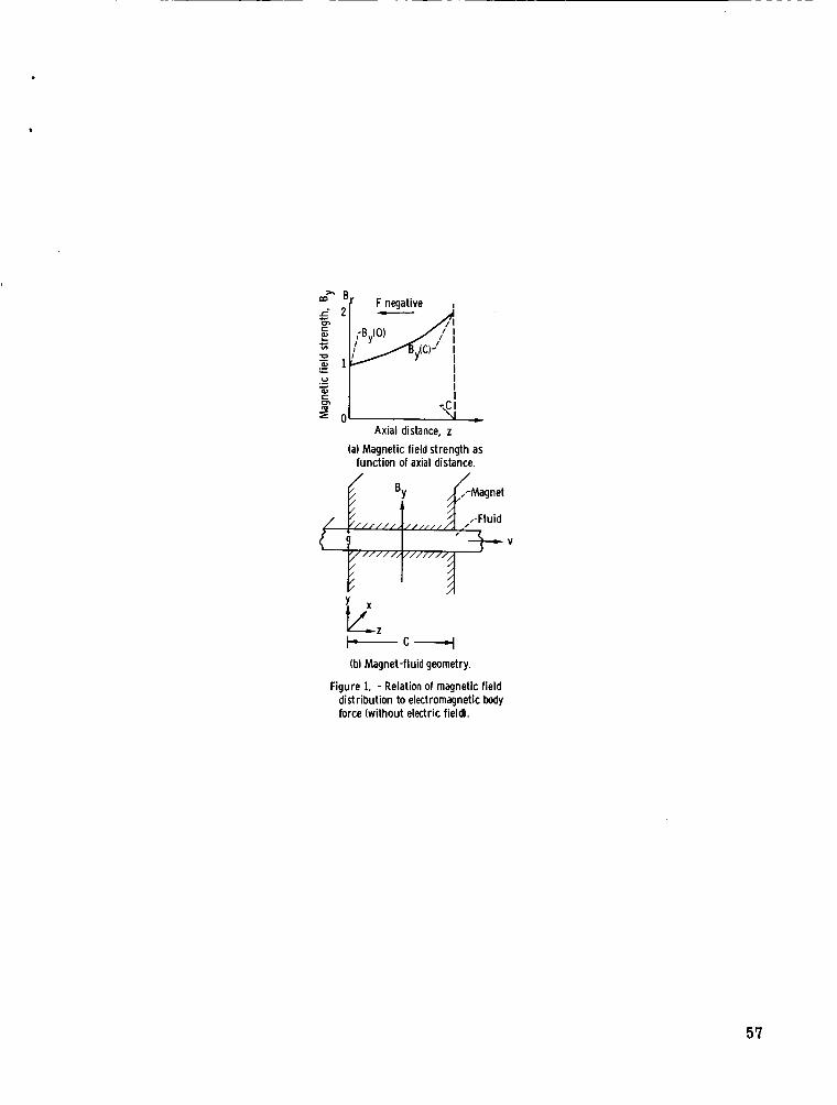
A plot of magnetic-field strength B against z is given in figure l(a) for a hypo- thetical case in which Co = 1 weber per square meter, and the flow magnetic Reynolds number Re,, = puvC = In 2. The total force exerted on the fluid can be computed by integrating the Lorentz force T X B’ over the volume occupied by the fluid:

Y

Total force * F = g / “ ( T X g ) d z 0

for a unit width in the x-direction.

4

Computing 7 from Ampere's law gives

.'

Theref ore,

= I [B2(0) - Bv(C$ 2 2p -

= Inlet magnetic pressure - Outlet magnetic pressure

2 2 2 Y where magnetic pressure is defined as the quantity B /2p. Note that, if B (0) > B (C),

then equation (11) states that j? is in the positive z-direction; whereas, if By(C) >By(0), a retarding force results. The sign of the force, therefore, depends only on the relative magnitudes of B2(0) and B2(C). For the situation depicted in figure l(a), B (C) > By(0)

and hence the force is negative. In the traveling-field electromagnetic pump, B (0) is made greater than B (C) by forcing the magnetic field to travel with a velocity vw that is in the same direction but has greater velocity than the fluid velocity v'. The relative velocity Gs = v' - v'

y 2 y 2

2 2

Y y 2 Y

2 Y, Y

is therefore negative, and equation (7) becomes W

-PLaVsZ = Coe

2 2 where v, = -V, and V, is a positive number. Equation (12) shows that B (0) > By(C). and a positive force results. For electromagnetic pumps in which current is supplied from an external source (conduction pumps), such a simple description as this is not possible; however, it can be shown that the magnetic pressure difference concept still holds. An example is given in appendix B.

The previous discussion and examples were presented in order to show that the electromagnetic body force can be thought of as the manifestation of an asymmetric magnetic field rather than as the interaction of electric and magnetic fields. The latter, perhaps, has more physical meaning, but the former point of view is more convenient for describing the principle of operation of the single-phase induction pump. The following sections show that the single-phase induction pumping principle results from bound- a r y conditions that cause the average magnetic pressure at pump inlet t o be greater than that at pump outlet, resulting in a positive pumping force.

.a Y I Y

1

Proposed Model and Assumptions

The systems to be analyzed are pictured in figure 2. In both cases a conducting fluid flows axially in an annulus bounded on either side by a core of high-permeability magnetic material. A radial, time-varying magnetic field, whose strength var ies both in time and space, is used to pump the fluid. Coils wound circumferentially around the low-radius portion of the magnetic core near the annulus inlet produce this magnetic field. Inlet and outlet pipes leading to and from the annulus may be either radial o r axial depending on which is more convenient.

Hereinafter, the configuration depicted in figure 2(a) will be referred to as type A and the configuration in figure 2(b) as type B. difference between the two configurations is that, in the type A pump, a low reluctance path for the magnetic field is provided at the annulus outlet side of the pump.

From figure 2 it is apparent that the only

The assumptions made in the analyses of these two pumps are as follows: (1) The magnetic field in the annulus has a component in the radial direction only. (2) The permeability of the magnetic core is much larger than that of free space. (3) Fringing of the magnetic field at each end of the annulus can be neglected. (4) All materials of the annulus, including the fluid, are isotropic, nonmagnetic,

(5) The magnetic field produced by electrical-current flow in the fluid outside the

(6) Electrical losses due to current flow in fluid outside the annulus are negligible. (7) The fluid in the annulus has a velocity component in the axial direction only. (8) Displacement currents can be neglected.

charge-free, and have a permeability equal to that of free space.

annulus is negligible.

6

The first of these assumptions should be valid as long as the annulus length in the axial direction is large as compared with the annulus width in the radial direction. The third assumption should be valid for large values of the ratio of annulus axial length to radial width. For very high values of the appropriate magnetic Reynolds numbers (defined in the next section), however, fringing at the annulus inlet is unavoidable. The results presented in this report are, therefore, limited to vflowff magnetic Reynolds numbers. The word"1ow" here does not necessarily mean less than 1 but is intended merely to indicate that fringing will become significant at some value of the appropriate magnetic Reynolds number. The fifth assumption should be valid if the fluid outside the annulus is not allowed to form a closed circumferential path in which induced current may flow. This stipulation can be accomplished either by using multiple inlet pipes o r by placing insulating baffles perpendicular to induced current flow in single inlet and outlet pipes. The sixth assumption is related to the fifth assumption and should also be valid if sufficient baffling, either by multiple pipes o r baffles, is provided.

Govern i ng Equation s

The analysis to be presented herein wil l be primarily concerned with determining the magnetic field in the pump annulus. The only consideration of the total magnetic circuit necessary will be that which is essential to determine the appropriate boundary conditions.

For the assumed configuration, a cylindrical coordinate system, as indicated in figure 3, is most convenient. Fluid velocity v' is given by

v'= vi

That the magnetic field has a component in the radial direction only has been as- +

sumed. Therefore, the magnetic field strength B can be written

B = Brg = Bg

(13)

Assuming axial symmetry ( a / M = 0) and a sinusoidal dependence of magnetic field strength 5 on time t produces

iwt B = d(r ,z )e

7

Equation (3) implies that

a - (rB) = 0 ar

Substituting fo r B from equation (15) yields the following:

This equation can be satisfied in general only if

a - (rat) = 0 ar

which implies that

Faraday's law (eq. (l)), axial symmetry, and equation (4) further require that

a - (rEe) = 0 ar

aEe - aB --- az at

ar az

- + - aEz - a (rEr) = 0 az r ar

Assuming also that Ee is sinusoidal in time yields

iwt Eo = y'(r, z)e

8

Equation (18) then implies

0

y'(r, z) = - Y (4 r

Equation (19) reduces to

- - - iwa! dz

(24)

Equations (20) and (21) suggest writing E, and E, as gradients of a potential function. For the case under consideration, however, no potential electric fields are applied, and since current flow in the annulus is uninterrupted by nonconducting dividers, none should arise. Therefore, the appropriate solutions for E, and E, a r e

E r = E z = O

In order to obtain the magnetic field strength B as a function of the axial coordinate z, Ampere's law, in integrated form, will be required. For the system under consideration, this form is

0

Equation (25) states that the line integral of the magnetic intensity H around a closed path P is equal to the electrical current flow through the area A enclosed by the path P. For the situation depicted in figure 3, the path P to be considered is the path abcd. The segments ab and cd a r e taken to be just long enough to enclose all material within the gap. Furthermore, segment ab is taken to be at the annulus inlet so that the magnetic intensity here is a function of radius and time only. Also, since the magnetic core has been assumed to have a permeability much higher than all other media in the annulus, the line integrals of the magnetic intensity H over paths bc and da are zero in comparison with the same integrals over paths ab and cd; that is,

4

Therefore, equation (25) reduces to

Before proceeding further, note that the only assumptions made about the materials in the gap are that they be isotropic, charge-free, and nonmagnetic. Any number of conducting, nonconducting, flowing, o r stationary materials is allowable, as long as the assumption of unidirectional magnetic field strength is valid. Figure 3 shows a typical case in which the pumped fluid and a cooling fluid flow in the annulus and are contained by four duct walls. For some situations, thermal insulation and several duct materials may be necessary. In general, assume n materials to be enclosed in the annulus, each with a conductivity a k and flowing with an axial speed Vk' From equation (5) it follows that the current density in the kth material is given by

*

4

From substituting equations (15), (17), (22), and (23), equation (27) becomes

Therefore, the total current passing through the area bounded by the path abcd is

n

j . d A = e 2 uk /rk+l lz [ y ( z ' ) + vk~(z')]dz'

*abed rk k= 1

f ' -

k= 1

The left-hand side of equation (26) can be evaluated by making the following substitu- t ions :

r

The ref o re,

10

Similarly ,

Inserting equations (29), (30), and (31) into equation (26) results in

+ Vk(Y(Z')ldZ'

Differentiating this equation twice with respect to the axial coordinate z and removing the factor eiot result in

Substituting for dy/dz in equation (24) gives

It is convenient at this point to define a flow magnetic Reynolds number Remv, a frequency magnetic Reynolds number Re,,, and a dimensionless axial coordinate (:

11

Rem, =

( = - Z

C

The inclusion of the factor 1/17 in the definilion of Re,, is explained in the section COMPARISON WITH TRAVELING-FIELD PUMPS and has to do with comparison of single-phase and traveling-field electromagnetic pumps.

With these definitions, equation (32) can be written

inRem,a, = 0 d2a, da, Remv - - -

dC2

The general solution to equation (36) is

where

r R e i = - 1 k e m v -

2 {,,,,,,,I

(34)

(35)

A convenient soh ion for the magnet c-field strength B is there,are possible by 4 .e - fining flow and frequency magnetic Reynolds numberd in the manner prescribed by equations (33) and (34). Remember, however, that these are average quantities and that in obtaining the solution given by equation (37) only the integral form of Ampere's law has

12

v

been used. Except in the ideal case where the only medium contained in the annulus is the fluid to be pumped, the differential form of Ampere's law will give a current density that is an average of the current densities of the various media in the annulus. The solution is therefore approximate. For more accurate computation of the current density in any particular material within the annulus, Ohm's law will be used. In this sense, the analysis presented herein is similar to analyses for which magnetic-Reynolds number ef - fects can be neglected. The difference is that the magnetic field B is not assumed but is obtained on the basis of the average magnetic Reynolds numbers Remv and Re,,.

#

-e

Boundary Conditions

After the form of the magnetic field as given by equation (37) is determined, appropriate boundary conditions must be assigned at the annulus inlet and outlet in order to determine the constants C1 and C2. A s a result of doing this for both pumps A and B, the magnetic and electric fields will be completely determined.

Substituting equation (37) into equation (24) and integrating with respect to ( give

For convenience, the complex constants C1 and C2 are defined in terms of two other complex constants K1 and K2 and the peak magnetic field strength Bc that exists in the low radius portion of the magnetic core on the inlet side of the annulus (see fig. 4). The magnetic-field strength Bc is assumed to be given by

iot i; - Bc = Bce

The definitions of the constants K1 and K2 are as follows:

C1 = KIBc

C2 = K2Bc

Therefore,

(39)

. and

iwt e iwCBce E = +- e ) B

r Re:

For both pumps A and B, the appropriate boundary condition at the annulus inlet is the same. This boundary condition is derived by taking the line integral of the electric field strength Ei at the annulus inlet around the closed paths 1A or 1B (see fig. 4). Faraday's law (eq. (1)) can then be used to relate the quantities Ei and Bc:

= -iwei& 1 Bc AC

+ 2nrEi = -iwB A c c

2 = -iwBc7ra

(43)

iwBc .2 E. 1 = - ____ r (T)

Equating equations (42) and (43) for 5 = 0 yields

2 (44)

For pump A, a second boundary condition is obtained by taking the line integral of

in the magnetic core on the outlet side of the annulus and the radial path the magnetic-field intensity around path 2A (see fig. 4(a)). Path 2A consists of the segment 2

rn+l outlet pipes has already been assumed. in

rl through the annulus at < = 1. That there is no current flow in the fluid or Therefore, using Ampere's law (eq. (2)) results

14

At { = 1

io t ; = Bc Re; eiwt; B = Boe - r (K1,Ae + K2, Ae

Therefore,

Re; 1

BC rl

- - - - K1, Ae + K2, Ae (45)

For most cases of interest, the quantity p/pc is generally much less than 1, and the right-hand side of equation (45) is approximately zero. Equation (45), therefore, can be approximated by

Re; Re: K1, Ae + K2,Ae = o

1,A Solving equations (44) and (46) simultaneously results in the following values of K and K2,A:

\ iRemom 2

iRem,m 2

Re; -Re:

Pump A

Re: -Re'

(47)

The second boundary condition for pump B is obtained by equating the line integral of the electric-field strength around path 2B to the negative rate of change of magnetic flux through the area enclosed by path 2B. Since no flux passes through this area, the appropriate boundary condition at { = 1 is that the electric-field intensity be zero. Therefore,

15

Re; K1,B e +- K2,B e = o Re& Re;

1, B Solving equations (44) and (48) simultaneously results in the following values of K and KZ,B:

If the excitation coil of either pumps A o r B is assumed to have N turns and carries a peak current 111, the number of excitation ampere-turns is

Again the use of Ampere's law to compute the line integral of the magnetic intensity around paths 3A o r 3B gives

- Bc ln[?) (K1 + K2) = NI c1

In deriving equation (51), the line integral of magnetic intensity over that portion of paths 3A o r 3B within the magnetic core has again been assumed small as compared with the magnetic intensity integral within the annulus. Also, current flow in the fluid and pipes on the inlet side of the annulus and fringing flux on both sides of the annulus have been neglected. Equation (51) provides a means f o r relating B, to the excitation ampere turns NI, o r vice versa. Since K1 and IC2 are complex, Bc and NT will, in general, have different phases. Equation (51), therefore, also determines either the phase of B, o r NI, given the phase of the other. The choice of Bc as a real number is convenient in order to simplify the equations resulting f rom the boundary conditions.

Comparison of equations (47) and (49) indicates that both pumps should have identical characteristics in the limiting case where R e k = -Re;. This behavior will occur, fo r

*

4

4

16

. instance, if Re,, is very high in comparison with Remv. Such circumstances result when the excitation frequency w is high and/or when the fluid velocity is low.

the magnetic field strength Bo at the outlet be zero. This boundary condition is not necessarily the case for pump B, except for high values of the ratio Rem,/Remv. Both pumps, however, have the same boundary conditions at the annulus inlet (eq. (44)). From the discussion presented in the first section and because the square of the outlet magnetic field strength BZ is a minimum (namely zero), pump A should be more capable of producing force than pump B. Because of these considerations, pump A is expected to have a higher ideal efficiency than pump B, which is, indeed, the case. Pump B, however, offers a simpler outlet duct construction and might be preferable in some instances.

# It is notable that, in pump A, the outlet boundary condition (eq. (46)) requires that

Performance Parameters

Some important parameters in the evaluation of electromagnetic pumps are efficiency, power factor, and peak magnetic-fjeld strength for a given pressure rise and flow rate. In order to determine the efficiency of single-phase pumps, the losses, electrical and viscous, which result from pump operation at the specified conditions must be determined. The electrical losses in the annulus and the peak magnetic-field strength Bc can be calculated from three dimensionless functions 9, x, and rc/, which will be defined in this section. Dimensionless core magnetic-field strength and power-factor functions will also be developed, from which calculations of the necessary excitation ampere-turns and voltage requirements can be made.

The real, dimensionless, functions bR(<), bI(<), e,(<), and e,(<) are defined so that

e R e i

(53)

Comparison of equations (52) and (53) with equations (41), (43), (47), and (49) shows that the functions bR(<), bI((), eR(<), and eI(c) depend only on < and the two magnetic Reynolds numbers Re,, and Remv. Magnetic and electric field strengths (eqs. (41) and (42)) can be written

and E

17

= - (%)A kR(c)cos ut - bI(c)sin r

(54)

In equations (54) and (55) the quantity B, has been taken to be a real number, and without loss of generality only the real part of Bc is considered to actually exist. It is

d d

therefore appropriate to take only the real par ts of B and E as defined in equations (41) and (42). The current density Tk in the k th medium within the annulus is

The amount of work done per unit time on medium k by the electromagnetic field is obtained by integrating the product of the Lorentz force per unit volume Tk X B' and the velocity Vk over the k that is, work done per unit time on medium k is

th volume and averaging the result over a period of time 2n/w;

. i

18

. Similarly, the electrical losses Lk in medium k are computed by integrating the

power losses ( j k - J 'k )/ok per unit Volume over the kth volume and taking the time average

The quantities cp, x, and J/ are dimensionless functions of the two magnetic Reynolds numbers Re,, and Remv and are defined as

(59)

The total work Wm done per unit time on all the media in the annulus is then

and, similarly, the total electrical loss Lm in the annulus is

19

n

k= 1

- Lm-

+.E k= 1

The developed pressure in the kth medium can be obtained from

For most pump designs, the peak f lux density in the magnetic core will occur in the low radius portion. The magnitude of Bc is, therefore, important in order to determine how close to saturation the pump is. A convenient nondimensionalization of Bc is provided by taking the line integral of the magnetic intensity around path 3A o r 3B (see fig. 4) and equating this to the excitation ampere turns N E Equation (50) can be written

Ni= (NIR COS Wt - NII sin ut)$ (65)

Again, only the real part of N T is used. Computing the line integral

d * B ' - - d2

'path 3A,B

and equating the result to equation (65), using equation (54), result in

20

BC

NI

a2 h(%+l)

Equation (68) defines p, a nondimensional peak magnetic-field strength, in te rms of the peak values of the low-radius core magnetic-field strength and the excitation ampere- turns. The quantities bR(0) and bI(0), and therefore 0, are functions of the two magnetic Reynolds numbers Remo and Remv only.

The voltage V necessary to produce a peak current I in an exciting coil of N turns can be computed from Ohm's law (eq. (5)). the sum of the applied potential field produced by V and the electric field Ei resulting f rom the presence of a time-varying magnetic field Bc. Since the velocity of the coils is zero, Ohm's law reduces to

The electric field % in this case is + -

21

4 4

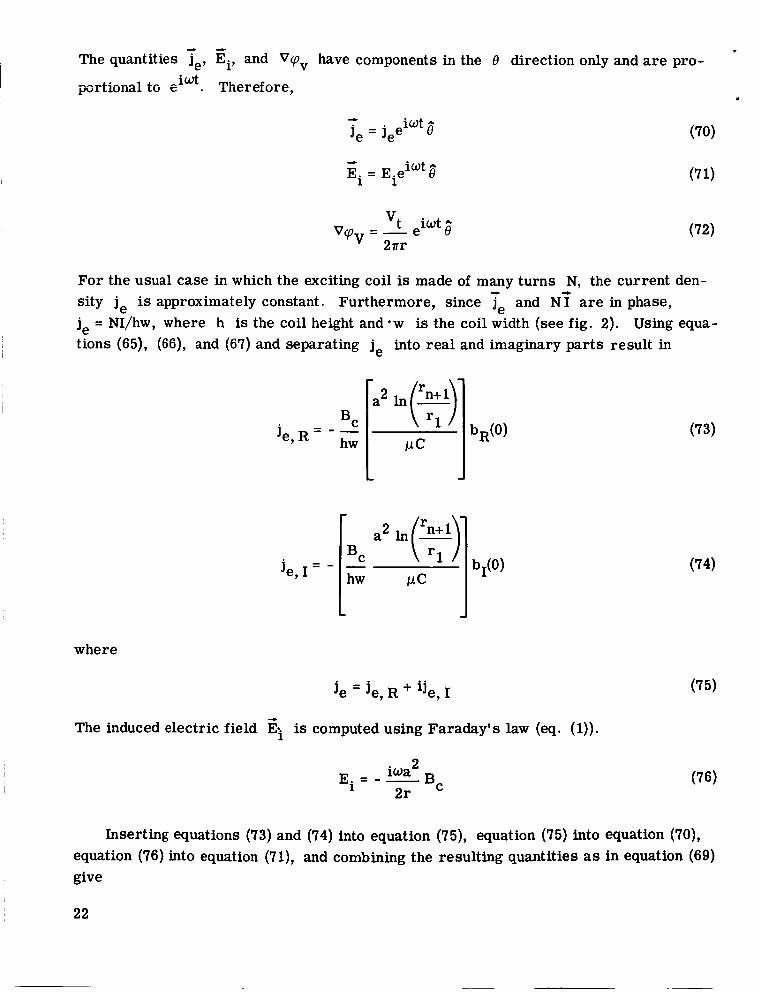
The quantities je, Ei, and V q v have components in the 8 direction only and are pro- .@rtioiia: to ,id. Thereffore,

i w t 8 E. = E.e 1 1

't eiwt; v'pv = 2nr

For the usual case in which the exciting coil is made of many turns N, the current density je is approximately constant. Furthermore, since Te and Ni are in phase, je = NI/hw, where h is the coil height and *w is the coil width (see fig. 2). Using equations (65), (66), and (67) and separating je into real and imaginary parts result in

I

where

The induced electric field is computed using Faraday's law (eq. (1)).

2 E. = -- i w a

2 r BC 1

Inserting equations (73) and (74) into equation (75), equation (75) into equation (70), equation (76) into equation (71), and combining the resulting quantities as in equation (69) give

22

[bR(0)cos ot - bI(0)sin hw

so that

2r

t - c i ‘e V - B COS Ut - - pChw

Defining a power factor function PFF such that

equation (77) becomes

na2 h(2) pChw

Vt = B, cos [

23

The quantity Vt defined in equation (77) is obviously the number of applied volts per turn of the coil. If turn 5 ef the C d has ii ineaii radius r and if all N turns are con- nected in series, then the voltage V that must be applied to the coils is

e, j

j= 1

The root-mean-square value of the voltage is

Besides the electrical losses in the fluid and duct walls, additional losses incurred in electromagnetic pumps are the coil electrical losses and the viscous losses resulting from the flow of the pumped fluid in the thin annulus. For constant coil current density je the coil electrical losses are

where re, is the minimum coil radius and r is the maximum coil radius. Substi- tuting equations (73) and (74) into equation (82) yields

e, 0

24

J If fluid flow in the annulus is turbulent, which is normally the case, and if the magnetic field in the annulus is not too strong, effects of the magnetic field on the viscous losses can be neglected. In this case, ordinary turbulent flow formula (ref. 3) can be used. If the Reynolds number Rek for the k th fluid in the annulus is defined as

a friction coefficient C can be found from the following f , k

'f, k = 3164 for 2(103) < Rek < lo5 Re:' 25

0.221 for Rek> 10 5

Re:. 237

Cf, = 0.0032 +

The viscous losses in the kth medium are

The total viscous losses are, therefore,

k= 1

The pressure drop in the kth medium is

25

It is understood that, if the kth medium is not a fluid, equations (87) and (89) have no meaning.

The efficiency of a particular pumping configuration is defined as the net amount of work done per unit time by the pump W divided by the input power 9 to the pump. The net amount of work done per unit time is the difference between the amount of work done by the electromagnetic field Wm and the viscous losses WH:

Since the input power to the pump is electrical in nature, 9 is the sum of the work done per unit time by the magnetic field Wm plus all the electrical losses incurred:

B = wm + Lm + Le

The efficiency is, therefore

77 = W - (100) = Wm - wH (100) 9 wm + Lm + Le

The aim of this section has been to develop equations that can be used to obtain the performance of single-phase pumps. Those parameters that are peculiar to the single- phase pumping concept have been given in dimensionless form. These dimensionless quantities, along with the physical and geometrical properties of the system, can be used to compute the real parameters that they represent. Other parameters of interest that do not depend on the electromagnetic field have been presented in dimensional form.

PERFORMANCE CHARACTERISTICS AND TRENDS

AS was shown previously in the ANALYSIS section, the performance of single-phase pumps depends largely on the two quantities Re,, and Remv. The question that remains is what is the criterion for the selection of these quantities so that a reasonably well-designed pump wi l l result. One criterion would be whether o r not pumping could be attained at the selected values of Rem, and Remv. Another might be a crude estimate of efficiency at various values of Rem, and Re,,, such as the ideal efficiency.

26

This section points out performance characteristics and trends for practical ranges of Re,, and Remv. Nondimensionalized curves of ideal output pressure (work), ideal efficiency, and peak core flux density are presented to provide crude estimates of performance. Finally, with these curves as a guide, nonideal performance effects are calculated for a sample pump.

.

Ideal Quantities

In obtaining a good pump design, obtaining the best efficiency compatible with a given developed pressure and flow rate is of primary interest. This section develops expressions for dimensionless developed pressure (work) and ideal efficiency so that best performance points can be estimated with relative ease.

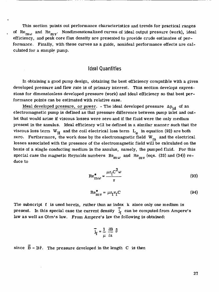
Ideal developed pressure, o r power. - The ideal developed pressure APid of an electromagnetic pump is defined as that pressure difference between pump inlet and outlet that would arise if viscous losses were zero and if the fluid were the only medium present in the annulus. Ideal efficiency will be defined in a similar manner such that the viscous loss term WH and the coil electrical loss term Le in equation (92) are both zero. Furthermore, the work done by the electromagnetic field Wm and the electrical losses associated with the presence of the electromagnetic field will be calculated on the basis of a single conducting medium in the annulus, namely, the pumped fluid. For this special case the mametic Re;mlcls numbers EP --mw and Re duce to

(eqs. (33) and (34)) remv

Re;,= pufvfC

The subscr& is used herein, rather than anindex k since only one medium is present. In this special case the current density jf can be computed from Ampere's law as well as Ohm's law. From Ampere's law the following is obtained:

- (94)

4

since B = Be. The pressure developed in the length C is then

27

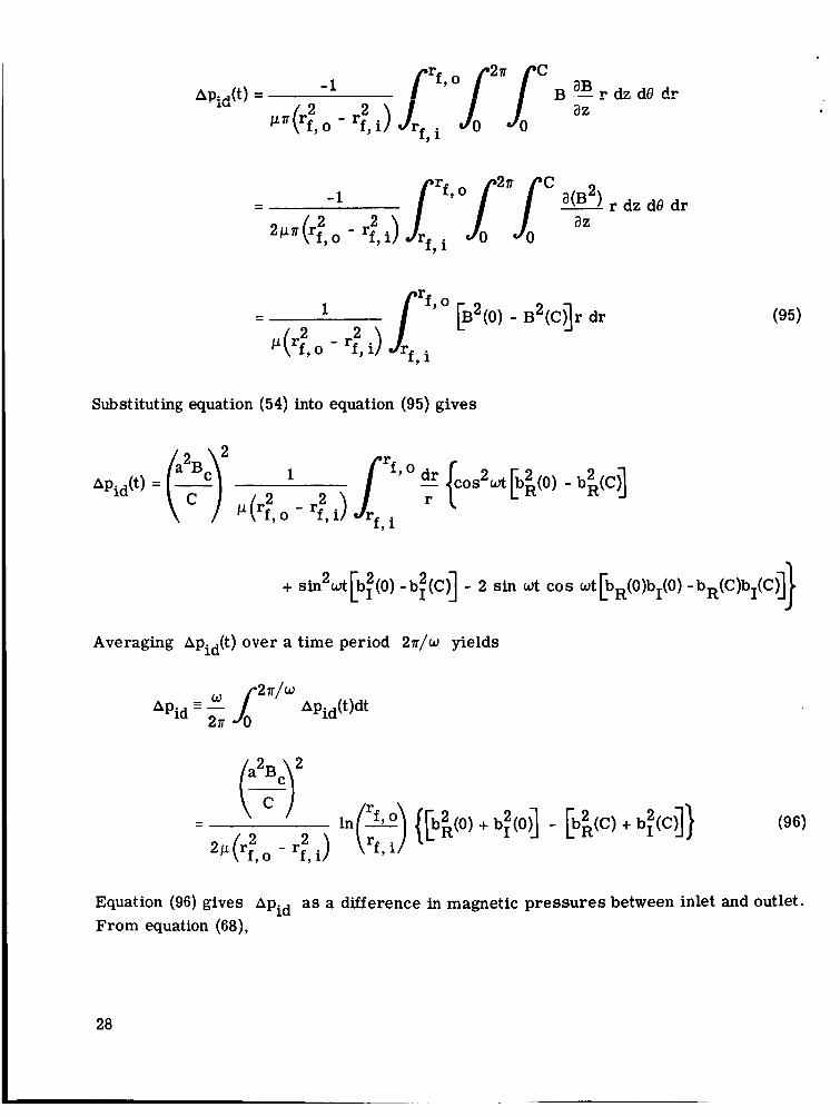
[B2(0) - B2(C)lr dr s rf'O 1 - -

2 .('t,o - r;, i) rf,

(95)

Substituting equation (54) into equation (95) gives

+ sin'wt [b;(O) - b;(C)l - 2 sin ot cos ut [bR(0)bI(O) - bR(C)bI(Cg 1 Averaging hpid(t) over a time period 2n/w yields

Equation (96) gives Apid as a difference in magnetic pressures between inlet and outlet. From equation (68),

28

Theref ore

LU

If a dimensionless output pressure A@id is defined so that

P

then by using equation (97), the following equation results:

The work done per unit time on the fluid by the electromagnetic field is

- Defining a dimensionless power Wid so that

- 2Wid h(E) Wid = n

clearly shows that

- Wid = ADid

Therefore, Apid can be thought of as either a dimensionless pressure rise o r a

frequency magnetic Reynolds number Re:, for several values of the flow magnetic Reynolds number ReLv. Figure 5(a) is somewhat more convenient for design calculations; whereas figure 5(b) can be thought of as a dimensionless-head - dimensionless- flow curve. Figure 5(b) is therefore useful in describing the approximate behavior of single-phase pumps in familiar te rms . Note that Apid is constant over the full range of Re:, fo r pump A. This behavior occurs because the quantity bR(C) + b;(C) is zero by virtue of the boundary condition at the annulus outlet as expressed by equation (46). this fact and substituting equation (68) into equation (99) give

d i m ~ n ~ l ~ n ! ~ ~ ~ n ~ t 2 ~ t p ~ e r . Figure 5 shciws diiiieiisioniess icieai pressure AP against id

2

Using

On the other hand, pump B exhibits a characteristic similar to that of a traveling- field electromagnetic pump. For this pump, a value of the frequency magnetic Reynolds number Re:, dependent on the flow magnetic Reynolds number ReLv exists, be- ( ),in low which pumping is not possible in the ideal case. A plot of (Re;,) of Re& is given in figure 6.

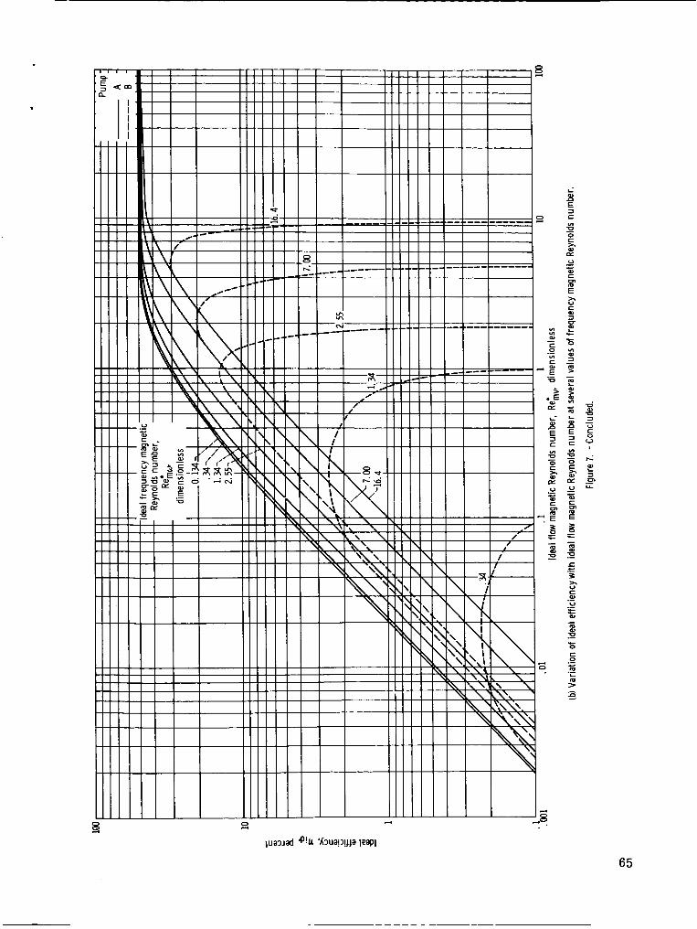
Ideal efficiency. - Figure 7 shows ideal efficiency qid against frequency magnetic Reynolds number Re;, for several values of the flow magnetic Reynolds number Re;,. Both figures 7(a) and (b) a r e given for the same reasons as given previously with regard to figures 5(a) and (b). Several trends inherent in these curves are worth noting.

First, both pumps A and B perform equally wel l f o r high values of the frequency magnetic Reynolds number Re;, (see fig. 7). This behavior results from the fact that the magnitudes of the complex magnetic Reynolds numbers R e k and Re; approach each other when Re,, becomes much largcr than Remv.

numbers greater than 1 in order to obtain reasonable efficiencies. For R e k v 5 1, values f o r ideal efficiency qid are less than 32 percent. Real efficiencies can be expected to be even less.

Thirdly, as Re:, is decreased, the ideal efficiency of pump B decreases and becomes zero at Re:, = Re:, . On the other hand, the ideal efficiency of pump A

approaches an asymptote as Re&, is decreased. Also, fo r sufficiently high values of R e k v this asymptote appears to approach its own asymptote of 7)id = 50 percent.

To determine whether these conclusions are correct, the ideal output power Wid and ideal electrical losses Lid in the fluid must be computed, and the values each of these approach as Re:, approaches zero must be determined.

as a function m in

Secondly, single -phase pumps apparently must be operated at flow magnetic Reynolds

( )min

( ) m a

30

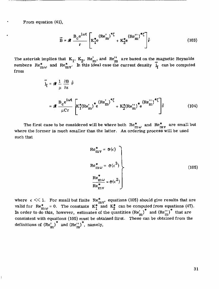
From equation (41),

*

The asterisk implies that K1, KZ, Re;, and Re: are based on the magnetic Reynolds numbers ReLu and Rehv. In this ideal case the current density jf can be computed from

e

The first case to be considered will be where both ReLu and Re&, are small but where the former is much smaller than the latter. An ordering process will be used such that

* Remv= @(E)

Re;u=

* -- - €Y(c2) Remu

Re;V

where E << 1. For small but finite ReLv, equations (105) should give results that are valid for R e z u = 0. The constants KT and K g can be computed from equations (47). In order to do this, however, estimates of the quantities (Rek) consistent with equations (105) must be obtained first. These can be obtained from the definitions of (Rek)

* * and (Re&) that are

* * and (Re;) , namely,

31

.

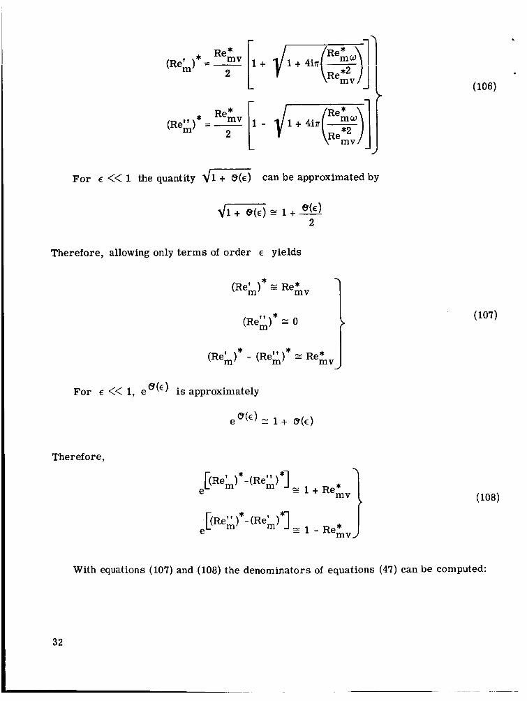
Therefore, allowing only terms of order E yields

i ...

L 'i

For E << 1 the quantity d G can be approximated by

For E << 1, e ' ( E ) is app:

Therefore,

.F

(ReA) =Re;$,

(Re,) ? ? * E O

* * (Re&) - (Re") m = Rehv

roximately

e a(E) 2 1 + O(E)

E l + R e m v

= 1 - Re;,

[(Reh)*-(Re" )*]

[(Re:)*- ( R e k ) I

e

e

With equations (107) and (108) the denominators of equations (47) can be computed:

32

I * * BRek) * - (Re'') *] (Re") - (Rek) e = 0 - Re&,(l + ReLv)

* I 1 * FRe")*-(Re&)*] = Remv * (Re;) - (Re,) e

Substituting equations (109) into equations (47) results in

I iRek ,na 2

iRe,,na * 2

* K " - 2CReLV(l + Re;$v)

K* e!

2 - 2CRekv

Using equations (107) and (110) in equations (113) and (114) results in

If

.-, Bcna2Rek, sin ot B Z S . (r - 1);

2Cr( 1 + Re:,)

Bcna 2 Re:, sin ut - j, S 2Cr(l + Re:")

then the ideal work Wid is given by

33

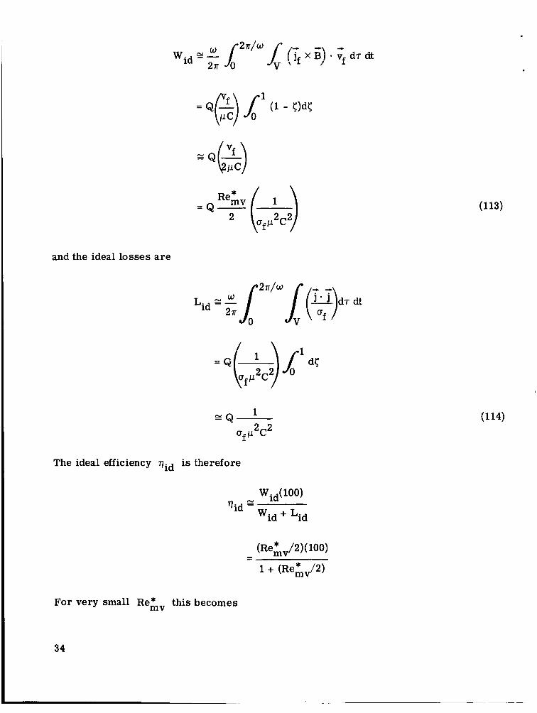
and the ideal losses are

= Q 1 2 2

0fl-l c

The ideal efficiency qid i s therefore

For very small Re;fiv this becomes

34

Re;,,( 100)

2 qid

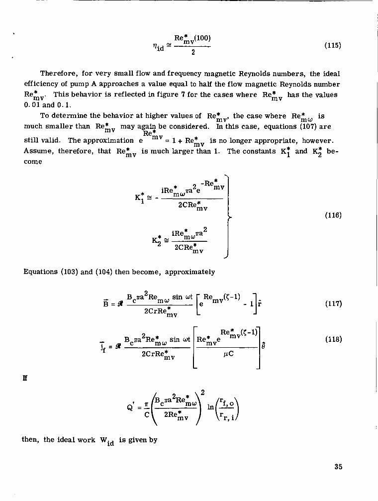
Therefore, for very small flow and frequency magnetic Reynolds numbers, the ideal efficiency of pump A approaches a value equal to half the flow magnetic Reynolds number Re&. This behavior is reflected in figure 7 for the cases where Re&v has the values 0.01 and 0.1.

To determine the behavior at higher values of ReLv, the case where Re&w is much smaller than Re& may again be considered. In this case, equations (107) are

= 1 + Rekv is no longer appropriate, however. still valid. The approximation e Assume, therefore, that Re;$, is much larger than 1. The constants KT and KZ become

Re&

* 2 * iRemona e K1 z -

* K2

Equations (103) and (104) then become, approximately

L J 2 C r R e i v

Bcra 2 Re&, sin Wt 4

j, = 9 2CrReGv

~

- li Re&,e

2 * Q'=-( 71 B c m Rem0 *

C 2RemV rr, i

then, the ideal work Wid is given by

35

-2Rekv -ReLv The t e rms containing e tion (119) since Re& >> 1. The ideal losses Lid are obtained from

and e have been neglected in computing equa-

In the limiting case of Re&, >> 1 and Re&w << 1, the work done on the fluid and the electrical losses in the fluid become of equal magnitude for pump A. Figure 7 shows that, in this h i t , the highest efficiencies are obtained. It can therefore be concluded that the maximum efficiency obtainable is 50 percent. By inference, this might seem a severe limitation in light of the fact that the maximum obtainable efficiency f o r traveling- field induction pumps is 100 percent. This conclusion is valid if the fluid electrical losses are much larger than other losses. If coil electrical losses are significant, however, which is quite often the case, highest efficiencies are usually obtained in those

36

pumps for which these losses a r e held at a minimum. The last section shows that the coil losses in single-phase induction pumps can be made considerably smaller than is possible in traveling-f ield pumps. This is possible primarily because coil temperatures and current densities can be made smaller.

Magnetic Flux Density Considerations

The value of the magnetic flux density Bc in the low-radius portion of the core is important for two reasons. First, if Bc is too large, the magnetic core is likely to saturate. Secondly, if Bc is large in comparison with the magnetic-field strength B' in the annulus, the magnetic intensity drop over those portions of paths 2A, 3A, and 3B that passes through the magnetic core is not necessarily zero (see fig. 4). Equations (46) and (51) would not, in this case, strictly apply. Saturation of the core will lead di- rectly to degraded performance. A nonzero magnetic intensity drop around paths 2A, 3A, and 3B will also lead to degraded performance since the required excitation ampere- turns (NI) will be larger, resulting in larger coil electrical losses. To calculate Bc would therefore be interesting in order to determine for a given pump configuration if any of these effects are important.

The dimensionless core magnetic flux density p (see eq. (68)) is shown in figure 8 as a function of frequency magnetic Reynolds number Rem, for several values of the flow magnetic Reynolds number Re,.. The curves for pump B are terminated at the point where (Re,,) =

_--

The section Ideal Quantities showed that for pump A the dimensionless pressure rise AFid was equal to 1 for all flow and frequency magnetic Reynolds numbers Re:, and

Since both APid and p are nondimensionalized with reference to excitation ampere-turns (NI), p gives a direct measure of the magnitude of Bc for a required Value of Apid. Figure 8 shows that p becomes large as Re,, becomes small. An approximate expression for small Re,, can be obtained by combining equations (51), (68), and (116):

From equation (121), p increases with increasing Remv and decreases with Re,,. From this it can be inferred that fo r low frequency excitation a very large core f l u density Bc is required. (At 0 = 0, equation (121) gives /3 = 00. This result is to be expected since a time-independent magnetic field should be incapable of producing a force

37

unless its strength is infinite. ) For small values of Remo, then, figures 5, 6, and 7 and all those to be presented hereinafter may not, he i d i d . JXIhether they i ire aiifficieiii io describe any particular single-phase pump will depend on the permeability of the magnetic core material, its saturation flux density, and the particular geometrical characteristics of the pump. For most single-phase pump designs, the method and curves presented herein should be sufficient to describe the performance. An example of the use of these curves to design a lithium radiator coolant pump is given in appendix C.

COMPARISON WITH TRAVELING-FIELD PUMPS

Because the single-phase pump is an induction pump, comparison of its performance with that of a traveling-field induction pump of similar geometry and operating characteristics is interesting. The analysis that will be used for computations of traveling-field pump performance is reported in reference 4. This analysis includes effects of fluid and duct wall conductivities on the distribution and magnitude of the two-dimensional magnetic field. Allowances are also made for viscous losses and coil electrical losses. The analysis is, however, restricted to many wavelength pumps and configurations for which only the first space and time harmonics of the magnetic field are important.

The analogy between single-phase and traveling-field pumps is depicted in figure 9. The i tems that are compared a r e given in table I.

The wavelength h in the traveling-field pump is made twice as long as the annulus length C in the single-phase pump because, over half a wavelength, the magnetic field in a traveling-field pump can be considered radially unidirectional. Since the magnetic field in the single-phase pump is radially unidirectional throughout the annulus C, the choice h = 2C provides a better analogy than h = C.

The choice of a single coil width of w/3 in the traveling-field pump is based on the assumption of six coils per wavelength in this pump. Therefore, over half a wavelength, the total coil width is 3(w/3) = w and the total coil size is the same for both the single- phase and traveling-field pumps. If the coil current density je is the same fo r both, which is assumed, then the coil electrical losses are the same.

is defined as follows: For the traveling-field pump, a dimensionless output pressure per wavelength APh

38

* where Apx is the output pressure over one wavelength and NIX is the peak ampere- turns per single coil. Equation (122) is to be contrasted with equation (98) for hjjid of the single-phase pump. If APX is defined as it was in equation (122), comparisons of APx and indicate the relative magnitudes of the output pressure developed fo r a given amount of coil loss. The factor 1/6 in equation (122) is necessary since the quantity (NIA)2/2 is proportional to the electrical loss in one coil only. In the traveling- field pump three-phase excitation and six coils per wavelength are assumed; hence, the total coil loss is proportional to 6(NIA)2/2.

Since the traveling-field pump analysis used allows two-dimensional effects to be included, APx as defined in equation (122) is not simply a function of Re,, and Remv as was the case for the single-phase pump, and if comparisons of Airid and ADx are to be made, a particular geometry for the traveling-field pump is necessary. The geometry to be chosen will be that of the example given in appendix C; namely,

*

rf, = 0.04575 m

r = 0.0491 m

h = 2C = 0.174 m

f , 0

Flow and frequency magnetic Reynolds numbers for a traveling-field pump will be taken so that

x 2

Remv = pavc = pav -

and

Re,, = pu(:)C = pu(---) hw h

From these equations, the slip S, defined as

Field speed - Fluid speed - - \2a / S = - Field speed

is given by

Thus, the ideal efficiency of the traveling-field pump is

= lOO(1 - S) = 100 ('TF)id

This function is plotted in figure 10 fo r the assumed value of Remv of 2.

assumed traveling-field pump configurations. Note that A$ reaches a peak at some value of ~e,, and then decreases, whereas Apid stays constant and (AFidk in-

creases with increasing Re,,. The drop in APA at high values of Re,, has been predicted and experimentally verified in reference 5 fo r rotating-field devices. This drop is due to the fact that at high values of (Re,, - Remv), magnetic field lines close by way of paths that are primarily in the flow direction. The body forces produced are therefore directed radially rather than axially. Furthermore, most of these field lines penetrate the surface of the fluid only (skin effect), which results in only a small net body force. Fo r situations in which only high-frequency excitation is available, a single-phase pump might therefore be desirable because of this dropoff behavior of traveling-field Pumps.

those of traveling-field pumps. Figure 10 shows curves of ideal and actual efficiency for traveling-field and single-phase pumps that satisfy the conditions outlined in apMn- dix C. The curves for the ideal efficiencies of the single-phase pumps are obtained di- rectly from figure 7(a). Each curve indicates how the efficiency of the particular pump it represents var ies with frequency magnetic Reynolds number if the output pressure is fixed at the design value by varying the magnitude of the excitation ampere-turns.

Curves of efficiency against Remw are given for a traveling-field pump of four wave- lengths. Comparisons of efficiencies of the four-wavelength traveling-field pump and the two single-phase pumps do not indicate that any one of these is substantially better for the application than any other. This conclusion is especially t rue if it is recalled that end effects have not been included in the traveling-field pump analysis and that a peak efficiency somewhat below that indicated in figure 10 will be the t rue efficiency. Further degradation in efficiency can also be expected because higher order space harmonics of the traveling field have not been included in the calculations.

A further inefficiency that may be present in the traveling-field pump resul ts if the coils cannot be kept at the design temperature of 589' K without unreasonable amounts of Cooling. If such is the case, then additional coil electrical losses can be expected because of increased resistivity of the coils. Cooling of the coils is, of course, also nec-

The quantities APid and AFA are plotted in figure 11 for both single-phase and the

OA

At high frequencies, efficiencies of single-phase pumps are, in general, greater than

The curves representing the single-phase pumps have been discussed previously.

40

essary in the single-phase pump but primarily for removing the heat generated electri- cally within the coils themselves. Heat transfer from the hot fluid to the coils can be prevented by simply locating the coils far from the fluid and duct. This cannot be done in the traveling-field pump since the coils must be as close to the duct as possible to minimize leakage flux across the slots.

Another advantage of the single-phase pump configuration is that the electrical loss in the coils can be made insignificant by increasing the dimension w (see fig. 9). The coil loss for a required number of ampere turns NI are given by equation (82) by using

b je = NI/hw:

2 W

Equation (128) shows that Le can be made as small as desired by increasing w. In a single-phase pump this can be done easily. In a traveling-field pump, w cannot be made arbitrarily large o r the higher order harmonics of the electromagnetic field produced will be sizeable. Also, if w is made too large the effective nonmagnetic gap is increased because of the large reluctance of the thin magnetic material between coils.

The coil loss Le in a traveling-field pump can be reduced by increasing coil height h rather than width w; however, they cannot be made arbitrarily small. This can be seen by taking the limit of equation (128) as h becomes infinite while w remains fixed:

IT 2 lim Le = - (NI) h-cw 2wue

In actuality, it is doubtful that even this limit can be approached since the leakage flux across the coils is a factor whose importance increases with increasing h and thereby reduces the flux passing through the fluid.

cient four-wavelength traveling-field pump is desirable at this point. An approximation is sufficient and so the pump weight is assumed equal to the product of the weight density of the magnetic material (magnet steel density 2 8.0lXlO kg/m3, o r 500 lb mass/ft ) and the total pump volume. Since the coils are of copper, which has a density approximately equal to that of steel, the approximation should be quite close to the actual weight Of the pump involved. In order to minimize the pump volume, all magnetic flux-carrying c ross sections a r e assumed to have the same area and this a rea is sufficient to allow 10 000 gauss to pass. The result of such a calculation yields a single-phase pump B mass of 19. 52 kilograms (43 lb) and a four-wavelength traveling-field pump mass of 34.50 kilograms (76 lb).

A comparison of the weights of the selected angle-phase pump B and the most effi-

t

3 3 4

41

The design efficiencies, excitation frequencies, and masses of the single-phase pump B (see appendix C) and four-wavelength traveling-field pump therefore are as follows:

Single-phase pump B:

q = 13.8 percent

0 = 1096 rad/sec (174.5 cps)

mass = 19.52 kg (43 lb)

Four-wavelength traveling-field pump:

= 16.0 percent

0 = 579 rad/sec (92.2 cps)

mass = 34.5 kg (76 lb)

SUMMARY OF RESULTS

Analyses of two types of single-phase induction pumps have been made and performance prediction methods have been outlined. Ideal and general performances of each have been discussed, and the following resul ts have been obtained:

scribed in t e rms of a flow magnetic Reynolds number Remv and a frequency magnetic Reynolds number Re,,. In the limit of very high values of Re,, and/or very low values of Re,., the performance of both pumps is the same.

2. Dimensionless quantities are defined from which calculations of the efficiency, magnetic core flux density, and voltage requirements of single-phase pumps can be made. Each of these dimensionless quantities is a function of both Re,, and Remv.

3. In the ideal case for which coil electrical, duct-wall electrical, and viscous losses are zero and only fluid electrical losses are included, the following conclusions can be made:

sure is independent of both Re;, and R e g v (asterisk refers to ideal quantities) and depends only on the annulus geometry and the magnitude of the excitation ampere-turns NI. The ideal efficiency decreases with Re;, and increases with Re;,. The ideal efficiency at low values of ReLv and Re:, can be shown to be approximately equal to 100 (Re&,/2), and the maximum value of the ideal efficiency is 50 percent. This

1. Performance of both single-phase electromagnetic pumps can be conveniently de-

a. Pump A (low-reluctance path at outlet): For this case, the ideal output pres-

42

' value is attained in the limit of zero Re:, and infinite Rekv.

b. Pump B (no low-reluctance path at outlet): This pump exhibits a characteristic similar to that of traveling-field pumps. There exists a minimum value of Re;,, referred to as Reg,

increases with increasing Re&,. As Re:, is increased from (Re;&) ( R e k J m i n m in at constant Re;, and NI, the ideal output pressure increases and approaches asymptot- ically the corresponding value of pump A. Similarly, the ideal efficiency increases, reaches a peak, and then approaches the ideal efficiency of pump A for the same Regv.

(1200' F) at a volume flow rate of output pressure of 10 Newtons per square meter (14.5 lb/in. ). By choosing maximum efficiency consistent with a maximum allowable core magnetic field strength, optimum efficiencies were found to be 14.1 percent for pump A and 13.8 percent for pump B. Be- cause the difference of 0.3 percentage points is small and since pump B offers a simpler duct construction, pump B is probably better for the application.

5. Comparisons of single-phase and traveling-field induction pumps show the single- phase pump to be potentially competitive o r superior in efficiency, reliability, and weight for the following applications:

'

, below which pumping is not possible. The value of ( 'min

4, 4. Single-phase pumps A and B were designed for pumping lithium at 922' K cubic meters per second (158 gal/min) and an

5 2

a. High-temperature applications b. High-flow, low -output-pressure applications c. Situations in which only high-frequency excitation is available

Lewis Research Center, National Aeronautics and Space Administration,

Cleveland, Ohio, November 18, 1966, 120-27-04-05-22. ~

43

APPENDIX A

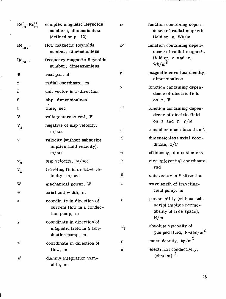
SYMBOLS

A

a

B

BS

b

C

cf

cO

cl’ c2

EaPP

Ei

E

e

F

g

H

44

2 area enclosed within path, m

radius of central magnetic core, m

magnetic field strength (without subscript implies radial com-

2 ponent), WB/m

effective magnetic core flux 2 density, Wb/m

complex function containing dependence of Br on (, Re,,, and Remv, dimensionless

annulus length, m

friction factor, dimensionless 2 integration constant, Wb/m

integration constants, Wb/m

electric field strength, V/m

electric field strength applied to conduction electromagnetic Pump, v/m

electric field strength at annulus inlet

complex function containing dependence of E on r, Rem,, and Remv, dimensionless

magnetic field, N force produced by electro-

gap height in conduction electromagnetic pump, m

magnetic field intensity, A/m

h

I

A

1

j

K1’ K2

i;

L

2

1 ,

N

NI

6

P

PFF

9

AP

Q Q’ Re

radial coil height, m

electric current per coil turn, A

unit vector in x-direction

electrical current density, A/m2

complex constants, m (see eq. (46))

unit vector in z-direction

power loss, W

dummy integration variable im- plying a differential portion of integration path, m

effective length of integration path in magnetic core, m

number of coil turns

number of coil ampere-turns

of the order of

path around which H is integrated

power factor function, dimensionless

power input, W

pressure rise, N/m

definedonp. 34, Wb /m

definedonp. 36, Wb /m

Reynolds number, dimension-

2

2

2

less

Re;, Re:

Remv

Rem w

9?

r

r A

S

t

V

vS

V

vS

vW

W

W

X

Y

Z

Z'

complex magnetic Reynolds numbers, dimensionless (defined on p. 12)

flow magnetic Reynolds number, dimensionless

frequency magnetic Reynolds number, dimensionless

real part of

radial coordinate, m

unit vector in r-direction

slip, dimensionless

time, sec

voltage a c r o s s coil, V

negative of slip velocity, m/sec

velocity (without subscript implies fluid velocity), m/sec

slip velocity, misec

traveling field or wave velocity, m/sec

mechanical power , W

axial coil width, m

coordinate in direction of current flow in a conduction pump, m

coordinate in direction'of magnetic field in a conduction pump, m

coordinate in direction of flow, m

dummy integration variable, m

CY

P

Y

Y'

E

77 n U

6 x

P

P

(5

function containing dependence of radial magnetic field on z, Wb/m

function containing dependence of radial magnetic field on z and r, m / m 2

magnetic core flux density, dim ension le s s

function containing dependence of electric field on z, V

function containing dependence of electric field on z and r, V/m

a number much less than 1

dimensionless axial coordinate, z/C

efficiency, dimensionless

circurr.ferential coordinate, rad

unit vector in 8-direction

wavelength of traveling- field pump, m

permeability (without subscript implies permeability of f ree space), H/m

absolute viscosity of

3

2 pumped fluid, N-sec/m

mass density, kg/m

electrical conductivity , (ohm/m)-'

45

7 dummy volume integration variable, m 3

cp, x, rc/ dimensionless functions defined in equations (59), (60), and (61)

magnetic flux, Wb

potential voltage, V pm

V V

0 frequency of excitation, rad/sec

Subscripts:

A

B

C

e

f

H

I

i

id

j

k

m

46

Pump A

Pump B

central magnetic core

exciting coils

pumped fluid

viscous losses

imaginary component of

for annulus, implies inner fluid radius; for coil, implies in- side radius

ideal

pertaining to jth coil turn

pertaining to kth medium in annulus

pertaining to electromagnetic field

min

n

0

R

r

r m s

TF

t

Y

h

e

minimum value

largest vahe fnr k

fo r annulus, implies outer fluid radius; for coil, implies outside radius

real component of

component in r-direction

root-mean-square value

traveling-f ield pump

pertaining to one coil turn

component in y-direction

value over one wavelength of traveling-field pump

component in 8 -direction

Superscripts : - vector quantity

defined for case where only fluid exists in annulus

*

- dimensionless

APPENDIX B

ELECTROMA'GNETIC BODY FORCE AS DIFFERENCE BETWEEN INLET AND

OUTLET MAGNETIC PRESSURES WHEN ELECTRIC FIELD capp IS APPLIED

2 2 0 Y Y

is assumed constant, equations (2) and (5) imply that

In the conduction electromagnetic pump B (0) is made greater than B (C) by the application of an electric field E in the positive x-direction. If all previous assumptions are made and E

0 aPP L aPP

- - - I aBy - a(vBy - Eapp) I-1 az

Equation (Bl) is solved by

Requiring again that

implies that

and

y v

Now c

For pumping operation, E is made large enough to ensure that aPP

47

The ref o r e,

under normal circumstances. Equation (17) can be written

B =-(1-Ke EaPP PUVZ) y v

2 2 Y Y

Applying the condition B (0) > B (C) results in a fairly complex relation of K and the flow magnetic Reynolds number Remv = povC. For reasonable values of K and

per square meter, K = 1/2, and Remv = In 2 is depicted in figure l(b). In this case

fig. 12).

this condition can usually be satisfied. The situation for which E v = 2 webers Remv a P d

B:(O) = 1 (Wb/m2)2 and BJ(C) 2 = 0 (Wb/m 2 2 ) , resulting in a positive pumping force (see

48

APPENDIX C

USE OF ANALYSIS AND RESULTANT CURVES FOR CALCULATING DESIGN

AND PERFORMANCE OF PARTICULAR PUMP APPLICATION

Figures 13, 14, and 15 give the dimensionless quantities q, x and @ as functions of frequency magnetic Reynolds number at several values of flow magnetic Reynolds number. These curves along with the dimensionless core flux density p (fig. 8) and the power factor function PFF (fig. 16) are sufficient to enable calculations of performance to be made with relative ease.

Consider the single-phase induction pump as the pumping unit for a lithium radiator coolant application and further assume that the required operating conditions are as follows:

Operating temperature = 922' K (1200' F)

Output pressure = 10 N/m (14.5 psi) 5 2

m3/sec (158 gal/min) Volume flow rate =

Fluid velocity = 10 m/sec (32.8 ft/sec)

Duct wali material = tantaium T - i l i at 922' K

Coils = Copper at 589' K (600' F)

7 2 Current density = 10 A/m

Core magnetic field strength = Bc 5 1.5 Wb/m 2

If it is assumed that only the pumped fluid, lithium, and two tantalum duct walls (see fig. 3) exist in the annulus, then subscripts 1 and 3 refer to the duct walls, and the subscript 2 re fers to the fluid. The important properties of the fluid and duct walls at 922' K are as follows:

6 1 a2 = 2.57X10 (ohm-m)-

= 470 kg/m3 (29. 5 lb/ft3) p2

Pf, 2 = 2 . 9 7 5 ~ 1 0 - ~ N-sec/m2 (2X10-4 Ib mass/ft-sec)

49

al = a3 = 2.07x10 6 (ohm-m)- 1

I 6 1 a, = 29. 7x10 (ohm-m)-

I

and the conductivity of copper at 589' K is

I Since the fluid velocity v2 is given as an input at 10 meters per second, the value of r3 can be obtained from

I r(ri - 4 ) v 2 = Volume flow rate

r [ . t - (0. 04575)2]1~ = 10- 2

~

Since the volume flow rate is cubic meter per second, it follows that ~

~

Further assume a duct-wall thickness of 0.00075 meter (0.03 in. ) and the following values of a, rl, r2, and w

a = 0.04 m (1.587 in. )

rl = 0.045 m (1.786 in. )

r2 = 0.04575 m (1.816 in.)

w = 0.03 m (0.01181 in. )

Solving for r3 in this equation yields

r3 = 0.0491 m (1.948 in. )

r4 = r3 + w = 0.04985 m (1.978 in.)

In order to determine the length C the flow magnetic Reynolds number Remv at which to operate must be specified. Figure 7 shows that if Remv is too small, the efficiency will be low. If Remv is chosen too high, Bc may be too high (refer to the discussion in the previous section). As a compromise choose

Remv = 2

50

If p = ~ T X I O - ' henry per meter (permeability of free space), the required length C can be computed from equation (33):

2 = c

r 4n(10-7) 2. 57(lO6)(lO)ln (-) 4 .91 In (- 4.985) 4.575

o r

C = 0.087 m (3.452 in. )

Since figure 7 indicates that pump A always has a higher ideal efficiency than pump B, pump A is the pump under consideration for this particular calculation. The value of Remo must now be chosen for pump A. If Re,, is chosen too high, the efficiency will be low. If Re,, is chosen too low, a value of Bc that is not permissible may be obtained. From figure 7, a reasonable value of Re,, seems to be 6.

tained from equation (34). The result is Using the computed value of C, the required excitation frequency can now be ob-

w = 822 rad/sec = 131 cps

At an Remv value of 2 and an Remo value of 6, figires 8, 13, 14, and 15 give

/3 = 0.550

cp = 0.057

x = 0.170

+ = 0.770

The required output power W can be computed from the values of output pressure and flow rate given as inputs:

W = (output pressure)(flow rate)

= 1000 w

51

Since the net output power W is the difference between the work done by the electromagnetic field Wm and the viscous losses L,, A I L, A L must first be computed in order to get the required value of Wm. The Reynolds number Re2 is obtained from equation (84): I

*

2(470)10(0.0491 - 0.04575) Re2 =

2. 975(10-4)

5 = 1.06X10

Using equation (86) gives a value for C of 0.0175. With th,3 value equations (87) f , 2

and (88) give

LH, 2 = LH

= 170 W

Therefore,

wm = LH + w

= 1000 + 170

= 1170 W

The required value of Bc can now be obtained from equation (62). The result of this calculation is a value fo r Bc of 1.247 webers per square meter, which is within the limit Bc 5 1.5 webers per square meter. Using this value of B, in equation (63) gives the total electrical losses Lm in the annulus of 5908 watts.

is NI = 3350 ampere-turns (peak value).

7 coil current density je is 10 amperes per square meter allows the necessary coil height h to be computed from

The required value of NI is obtained from equation (73) for p = 0. 550. The result

Assuming a coil width w of 0.03 meter (1 .191 in. ) and recalling that the required

3350 - - lo7 3(10-2)

E 1 . 1 2 ~ 1 0 - ~ m (0.438 in. )

52

If the minimum coil radius re, is made to be the same as the radius a of the low- radius portion of the core, then the maximum radius of the coil r is e, 0

re, o = re, i +

= 0.04 + 0.0112

= 0.0512 m (2.025 in. )

Using equation (82) to compute the coil losses results in Le = 162 watts. The total input power 9 is the sum of Wm, Lm, and Le:

B = wm + Lm + Le

= 1170 + 5908 + 162

= 7340 W

The efficiency 7 is therefore

- 1000 - - 100 7240

= 13.8 percent

This value of efficiency, of course, is not necessarily the best obtainable under the conditions of operation imposed. Better efficiencies could conceivably be obtained at higher o r lower values of the flow and frequency magnetic Reynolds numbers. Other parameters such as fluid velocity and dimensions might also be varied. Figure 10 shows how efficiency varies with Re,, if the values of Remv, je, w, a, rl, r2, r3, r4, and C are held fixed. This is done f o r both pumps A and B for the volume flow rate of

cubic meter per second and output pressure of 10 newtons per square meter. The efficiency of pump A remains relatively constant to a frequency magnetic Reynolds num - ber of approximately 7 and decreases with Re,, slowly. The section Magnetic Flux Density Considerations showed that, for very low values of Rem,, the necessary value of Bc for a given output pressure and flow is large. Therefore, the selection of a pump operating frequency will be based on maximum efficiency consistent with an inner core field strength Bc which is less than o r equal to 1.5 webers per square meter.

5

53

Figure 17 shows how the required value of Bc varies with Remw for both pumps A and B. For pump A, the lowest p r m i s s i b k -mke d Tte is approximately 4.65, mw whereas for pump B, Re,, E 5.375 is the minimum value. At the Re,, value of 4.65, figure 10 gives an efficiency for pump A of approximately 14.1 percent. Since efficiency decreases as Remw increases, this represents the best efficiency obtainable in pump A for the particular conditions considered. For pump B, however, the best efficiency is not obtained at the point where Bc = 1.5 webers per square meter, but peaks at an Re,, value of approximately 8. At this value of Remw the efficiency is approximately 13.8 percent, and Bc is approximately 1 weber per square meter. The efficiencies, required excitation frequencies, and required core magnetic field strengths Bc for pumps A and B at design conditions are therefore:

Pump A:

77 = 14.1 percent

w = 637 rad/sec = 101.3 cps

Bc = 1.5 Wb/m 2

Pump B:

77 = 13.8 percent

w = 1096 rad/sec = 174.5 cps

Bc = 1.0 Wb/m 2

Therefore, for the particular application considered and for an Remv of 2, the optimum efficiencies of pumps A and B are not greatly different. Since pump B of fers a simpler hydraulic design, this pump would probably be chosen and the 0.3 percentage points difference in efficiency sacrificed.

54

REFERENCES

1. Verkamp, J. P. ; and Rhudy, R. G. : Electromagnetic Alkali-Metal Pump Research Program. NASA CR-380, 1966.

2. Watt, D. A. : A Single Phase Annular Induction Pump for Liquid Metals. Rep. No. AERE-ED/R- 1844, Atomic Energy Research Establishment, Great Britain, Jan. 21, 1953. (Declassified version of AERE -CE/R-1090. )

3. Vennard, J. K. : Elementary Fluid Mechanics. John Wiley & Sons, Inc., 1947, pp. 157- 161.

4. Schwirian, Richard E. : Analysis of Linear-Induction o r Traveling-Wave Electro- magnetic Pump of Annular Design. NASA TN D-2816, 1965.

5. Schwirian, Richard E. : Effect of Magnetic Reynolds Number in Rotating MHD Induc- tion Machines. M. S. Thesis, Case Institute of Technology, 1964.

55

56

TABLE I. - COMPARISON O F SINGLE- PHASE AND

TRAVELING-FIELD PUMPS

Dimensions and conditions

Fluid temperature , OK c o i l temperature , OK Annulus length Inner fluid radius Outer fluid radius Coil height Coil width Coil cur ren t density Flow magnetic Reynolds number

jingle- phase

922 589 C

'f, i

f , 0 r

h W

Je 2

Pump

Traveling-field

922 58 9

112 wavelength X

rf, i

h f f , 0

w/3

Je 2

.

c m

Axial distance, z (a) Magnetic field strength as

function of axial distance.

(b) Magnet-fluid geometry,

Figure 1. - Relation of magnetic field distribution to electromagnetic body force (without electric field).

57

1

Annulus outlet - Magnetic core -. Annulus inlet -

3

Coil -

(b) Pump B, zero electric field outlet

,-Low reluctance path

CD-8779

Magnetic core

Annulus Total

Pumped fluid

- , J4-

I I

Magnetic core I 1

1

TT

Figure 3. - Analytical model of annulus.

59

Coi I

Possible fringing flux

(a) Pump A, zero magnetic field outlet.

Coil -.

(bl Pump B. zero electric field outlet.

,-Path 3B

,- Path 1 B

,,- Possible fringing flux

7 Flux ' lines

Figure 4. - Derivation of boundary conditions.

-Path 3A

--Path 1A

-Flux linec

,-Bo

,Path 2A (length. 1,)

CD-8778

60

1 le 100 Ideal frequency magnetic Reynolds number, Re*w dimensionless

(a) Variation of dimensionless ideal pressure, ,or output p e r , with ideal frequency magnetic Reynolds number.

Figure 5. - Dimensionless ideal pressure, or output pmver, for single-phase induction pumps of zero magnetic field and zero electric field outlet.

61

5 c UI U 0 c ZI a2 w U

a2

-

.-

.I-

f - B

.- 8

.- 5

H

- - B L-

c 3

3 0

n c

8 W- L =I VI VI a2 L n - .- 2 UI VI W

c 0

c

- .- VI

.- E U

0 c 0 - m L m

- .- .- > e

.

4 - U c 0

u

ui t 3 m Y .-

62

Figure 6. -Variation of ideal flow magnetic Reynolds number with minimum ideal frequency magnetic Reynolds number.

63

64

. T

a

65

8 r(

66

(a) Single-phase pump configuration.

J

i I I Flow-

I I I I

(b) Similar traveling-field pump configuration.

Figure 9. - Comparison of single-phase and traveling-field electromagnetic pumps.

67

Figure 10. - Overall and ideal efficiencies of single-phase (pumps A and B) and traveling-field electromagnetic pumps. Fluid, lithium; temperature, 922" K (1200" F); flow rate, Output Pressure, lo5 newtons per square meter (14.5 psi); flow magnetic Reynolds number, 2.

cubic meters per second (1% gallminl;

9 10 " -

2 3 4 5 6 r a Frequency magnetic Reynolds number, Re, dlmensionless

Figure 11. - Dimensionless o@@t pressure d single-phase and travellng-fleld dectromagnetlc pumps. Fluid, lithium; bmpera- ture, 922" K (1200" F); flw rate, 1 cubic meters per second

(14.5 psi); flow magnetic Reynolds number, 2. (1% gallmin); output pressure, 1 8" newtons per square meter

69

F Positive - .

0 C

(a) Magnetic field strength as function of axial distance.

CD-8777

(b) Magnet-fluid geometry.

Figure 12. - Relation of magnetic field distribution to electromagnetic body force (with electric field).

70

,

4 0 N 0

VI VI al

c 0 VI c

- .- E .- V

2

f

al 0:

L- al n

3 c VI '0

0 c )r al

lx U

0)

-

.- c

p A U c al 3 0-

U E

- m V

E a

2

VI n E

c

c al

3 0 U al

V L c V al

aJ

-

- .- - .- - e al N

V c W

V 0)

V

al c Ol

- .- - .- c

2 e

2

al N

0 - f n c 0

U 3 U c

al VI m

.- c

.-

5 al Ol c VI L

- .- e c 0

V c 3

.- c

L: 9

5 E 2 0,

Y .-

71

72

Figure 15. - $-Function for single-phase induction pumps A and B with zero magnetic field and zero electric field outlet.

73

c

c 01

3 0 FI 01

U

- - .- L

I-

P 01

E al N u c m al

V

al

.- c

.- c

!! e a N

.- 5 iz m U c m 6 v) a z s .- 4

2 U c .- c al

rn c VI L c

e - .- 0

c 0 .- P

8

:

3 ..- L

e L

n

9 e a rn U .-

74

NASA-Langley, 196'7 - 25 E-3131

Figure 17. - Required core magnetic field strength of single-phase electromagnetic pumps A and B Fluid, lithium; temperature, 922" K (1200" F); flow rate, lo-* c bic meters per second

(14.5 psi); flw magnetic Reynolds number, 2. (158 gallmin); output pressure, 1 2 newtons per square meter

75

“The aeronautical and space actiuities of the United States shall be conducted so as to contribate . . . to the expansion of human knowledge of Phenomena in the atmosphere and space. The Administration shall provide for the widest practicable and appropriate dissemination of information concerning its activities and :he results tbereof.”

-NAnONAL AaR0NAUnC.S AND SPACE ACT OF 1958

NASA SCIENTIFIC AND TECHNICAL PUBLICATIONS

TECHNICAL REPORTS: Scientific and technical information considered important, complete, and a lasting contribution to existing knowledge.

TECHNICAL NOTES: Information less broad in scope but nevertheless of importance as a contribution to existing knowledge.

TECHNICAL MEMORANDUMS: Information receiving limited distribution because of preliminary data, security classification, or other reasons.

CONTRACTOR REPORTS: Scientific and technical information gen-ted under a NASA contract or grant and considered an important contribution to

TECHNICAL TRANSLATIONS: Information published in a foreign language considered to merit NASA distribution in English.

SPECIAL PUBLICATIONS: Information derived from or of value to NASA activities Publications include conference p’y~eediugs, monograph, data compilations, handbooks, sourcebooks, and special bibliographk

TECHNOLOGY UTILIZATION PUBLICATIONS Information on technology used by NASA that may be of particuliu interest in commercial and other noa-aerospace applications. Publications include Tech Briefs, Technology Utilization Reports and Notes, and TBchaology Surveys.

existing knowledge.

hta i ls on the availability of these publications may be obtained horn:

SCIENTIFIC AND TECHNICAL INFORMATION DIVISION

N AT1 0 N A L A ER 0 N A UTI CS A N D SPA C E A D M I N I ST R AT IO N

Washington, D.C 90546

Documents

SINGLE-PHASE INDUCTION - NASA of single-phase induction pumps is largely dependent on two dimension- less quantities, flow magnetic Reynolds number and frequency magnetic Reynolds